Computational Fluid Dynamics (CFD, CHD)*PDE (Shocks 1st); Part I: Basics, Part II: Vorticity Fields

Rubin H Landau

Sally Haerer, Producer-Director

Based on A Survey of Computational Physics by Landau, Páez, & Bordeianu

with Support from the National Science Foundation

Course: Computational Physics II

1 / 1

Problem: Placement of Boulders for Migrating Salmon

Wake Block “Force” of River?

surface

bottom bottom

surfaceRiver River

xx

yy

L

HL

Deep, wide, fast-flowing streams

“Boulder” = long rectangular beam, plates

Objects not disturb surface/bottom flow

Problem: large enough wake for 1m salmon2 / 1

Theory: Hydrodynamics

Assumptions; Continuity Equationsurface

bottom bottom

surfaceRiver River

xx

yy

L

HL

∂ρ(x, t)∂t

+ ~∇ · j = 0 (1)

j def= ρ v(x, t) (2)

(1): Continuity equation1st eqtn hydrodynamicsIncompressible fluid

⇒ ρ = constantFriction (viscosity)Steady state, v 6= v(t)

3 / 1

Navier–Stokes: 2nd Hydrodynamic Equation

Hydrodynamic Time Derivative

DvDt

def= (v · ~∇)v +

∂v∂t

(1)

For quantity within moving fluid

Rate of change wrt stationary frame

Velocity of material in fluid element

Change due to motion + explicit t dependence

Dv/Dt : 2nd O v ⇒ nonlinearities

∼ Fictitious (inertial) forces

Fluid’s rest frame accelerates4 / 1

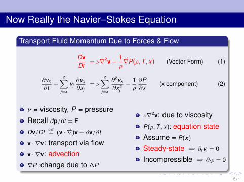
Now Really the Navier–Stokes Equation

Transport Fluid Momentum Due to Forces & Flow

DvDt

= ν∇2v− 1ρ~∇P(ρ,T , x) (Vector Form) (1)

∂vx

∂t+

z∑j=x

vj∂vx

∂xj= ν

z∑j=x

∂2vx

∂x2j− 1ρ

∂P∂x

(x component) (2)

ν = viscosity, P = pressureRecall dp/dt = F

Dv/Dt def= (v · ~∇)v + ∂v/∂t

v · ∇v: transport via flowv · ∇v: advection~∇P :change due to ∆P

ν∇2v: due to viscosityP(ρ,T , x): equation stateAssume = P(x)

Steady-state ⇒ ∂tvi = 0

Incompressible ⇒ ∂tρ = 0

5 / 1

Resulting Hydrodynamic Equations

Assumed: Steady State, Incompressible, P = P(x)

~∇ · v ≡∑

i

∂vi

∂xi= 0 (Continuity) (1)

(v · ~∇)v =ν∇2v− 1ρ~∇P (Navier–Stokes) (2)

(1) Continuity equation: Incompressibility, in = outStream width� beam z dimension ⇒ ∂zv ' 0 ⇒

∂vx

∂x+∂vy

∂y= 0 (3)

ν

(∂2vx

∂x2 +∂2vx

∂y2

)= vx

∂vx

∂x+ vy

∂vx

∂y+

1ρ

∂P∂x

(4)

ν

(∂2vy

∂x2 +∂2vy

∂y2

)= vx

∂vy

∂x+ vy

∂vy

∂y+

1ρ

∂P∂y

(5)6 / 1

Boundary Conditions for Parallel Plates

Physics Determines BC ⇒ Unique Solution

L

H

Constant stream velocity +Low V0, high viscosity ⇒Laminar: smooth, no cross⇒ streamlines of motionThin plates ⇒ laminar flow

Upstream unaffectedSolve rectangular regionL,H � Rstream ⇒ uniformdownFar top, bot ⇒ symmetry

7 / 1

Analytic Solution for Parallel Plates (See Text)

Bernoulli Effect: Pressure Drop Through Platessurface

bottom bottom

surfaceRiver River

xx

yy

L

HL

vx (y) =1

2ρν∂P∂x

(y2 − yH) (1)

∂P∂x

= known constant (2)

V0 = 1 m/s, ρ = 1 kg/m3, ν = 1 m2/s,H = 1 m (3)

⇒ ∂P∂x

= −12, vx (y) = 6y(1− y) (4)

8 / 1

Finite-Difference Navier–Stokes Algorithm + SOR

Rectangular grid x = ih, y = jh

3 Simultaneous equations→ 2 (vy ≡ 0)

v xi+1,j − v x

i−1,j + v yi,j+1 − v y

i,j−1 = 0 (1)

v xi+1,j + v x

i−1,j + v xi,j+1 + v x

i,j−1 − 4v xi,j (2)

=h2

v xi,j[v x

i+1,j − v xi−1,j

]+

h2

v yi,j

[v x

i,j+1 − v xi,j−1

]+

h2

[Pi+1,j − Pi−1,j ]

Rearrange as algorithm for Successive Over Relaxation

4v xi,j = v x

i+1,j + v xi−1,j + v x

i,j+1 + v xi,j−1 −

h2

v xi,j[v x

i+1,j − v xi−1,j

]− h

2v y

i,j

[v x

i,j+1 − v xi,j−1

]− h

2[Pi+1,j − Pi−1,j ] (3)

Accelerate convergence + SOR; ω > 2 unstable

9 / 1

End Part I: Basics

surface

bottom bottom

surfaceRiver River

xx

yy

L

HL

10 / 1

Part II: Vorticity Form of Navier–Stokes Equation

2 HD Equations in Terms of Stream Function u(x)

~∇ · v = 0 Continuity (1)

(v · ~∇)v = − 1ρ~∇P + ν∇2v Navier–Stokes (2)

Like EM, simpler via (scalar & vector) potentials

Irrotational Flow: no turbulence, scalar potential

Rotational Flow: 2 vector potentials; 1st stream function

v def= ~∇× u(x) (3)

= ε̂x

(∂uz

∂y− ∂uy

∂z

)+ ε̂y

(∂ux

∂z− ∂uz

∂x

)(4)

~∇ · (~∇× u) ≡ 0 ⇒ automatic continuity equation11 / 1

2 HD Equations in Terms of Stream Function (cont)

2-D flow: u = Constant Contour Lines = Streamlines

v def= ~∇× u(x) (1)

= ε̂x

(∂uz

∂y− ∂uy

∂z

)+ ε̂y

(∂ux

∂z− ∂uz

∂x

)(2)

vz = 0 ⇒ u(x) = uε̂z (3)

⇒ vx =∂u∂y, vy = −∂u

∂x(4)

12 / 1

Introduce Vorticity w(x) ∼ ~ω

Vortex: Spinning, Often Turbulent Fluid Flow

w def= ~∇× v(x) (1)

wz =

(∂vy

∂x− ∂vx

∂y

)(2)

Measure of ~v ’s rotation

RH rule fluid element

w = 0 ⇒ irrotational

w = 0 ⇒ uniform

Moving field lines

Relate to stream function:

13 / 1

Introduce Vorticity w(x) ∼ ~ω

∼ Poisson’s equation ∇2φ = −4πρ

x

y

0

12

6

40 80

w(x,y)

xy

0

-1

0

50 0

20

w def= ~∇× v(x) (1)

w = ~∇× v = ~∇× (~∇× u) = ~∇(~∇ · u)−∇2u (2)

yet u = u(x , y)ε̂z ⇒ ~∇ · u = 0 (3)

⇒ ~∇2u = −w (4)

Like Poisson with ea w component = source

14 / 1

Vorticity Form of Navier–Stokes Equation

Take Curl of Velocity Form

~∇×[(v · ~∇)v = ν∇2v− 1

ρ~∇P (Navier–Stokes)

](1)

ν∇2w = [(~∇× u) · ~∇]w (2)

In 2-D + only z components:

∂2u∂x2 +

∂2u∂y2 = − w (3)

ν

(∂2w∂x2 +

∂2w∂y2

)=∂u∂y

∂w∂x− ∂u∂x

∂w∂y

(4)

Simultaneous, nonlinear, elliptic PDEs for u & w

∼ Poisson’s + wave equation + friction + variable ρ15 / 1

Relaxation Algorithm (SOR) for Vorticity Equations

x = ih, y = jhCD Laplacians, 1st derivatives

ui,j =14

(ui+1,j + ui−1,j + ui,j+1 + ui,j−1 + h2wi,j

)(1)

wi,j =14

(wi+1,j + wi−1,j + wi,j+1 + wi,j−1)− R16{[ui,j+1 − ui,j−1]

× [wi+1,j − wi−1,j ]− [ui+1,j − ui−1,j ] [wi,j+1 − wi,j−1]} (2)

R =1ν

=V0hν

(in normal units) (3)

R = grid Reynolds number (h→ Rpipe); measure nonlinearSmall R: smooth flow, friction damps fluctuationsLarge R (' 2000): laminar→ turbulent flowOnset of turbulence: hard to simulate (need kick)

16 / 1

Boundary Conditions for Beam

Ou

tle

t

dw/dx = 0

du/dx = 0vx = du/dy = V0

w = 0

Inle

t

HalfBeam

Surface

vx = du/dy = V0 w = 0

y

x

vy = -du/dx = 0

center line

w = u = 0 w = u = 0

u = 0

u = 0

vy = -du/dx = 0

A

B

C

E

F

G

H

D

Well-defined solution of elliptic PDEs requires u, w BCAssume inlet, outlet, surface far from beamFreeflow: No beamNB w = 0 ⇒ no rotationSymmetry: identical flow above, below centerline, not thru

17 / 1

Boundary Conditions for Beam (cont)

See Text for More ExplanationsCenterline: = streamline, u = const =0 (no v⊥No flow in, out beam to it ⇒ u = 0 all beam surfacesSymmetry ⇒ vorticity w = 0 along centerlineInlet: horizontal fluid flow, v = vx = V0:Surface: Undisturbed⇒ free-flow conditions:Outlet: Matters little; convenient choice: ∂xu = ∂xwBeamsides: v⊥ = u = 0; viscous ⇒ v‖ = 0Yet, over specify BC ⇒ only no-slip vorticity w :Viscosity ⇒ vx = ∂u

∂y = 0 (beam top)

Smooth flow on beam top ⇒ vy = 0 + no x variation:

∂vy

∂x= 0 ⇒ w = −∂vx

∂y= −∂

2u∂y2 (1)

Taylor series ⇒ finite-difference top BC:

w ' −2u(x , y + h)− u(x , y)

h2 ⇒ wi,j = −2ui,j+1 − ui,j

h2 (top) (2)

Likewise for other surface:

r@ c@ @ lr@ c@ l@ lu = 0; w = 0Centerline EA(3)

u = 0, wi,j =− 2(ui+1,j − ui,j )/h2 Beam back B(4)

u = 0, wi,j =− 2(ui,j+1 − ui,j )/h2 Beam top C(5)

u = 0, wi,j = −2(ui−1,j − ui,j )/h2Beam front D(6)

∂u/∂x = 0, w =0 Inlet F(7)

∂u/∂y = V0, w = 0Surface G(8)

∂u/∂x = 0, ∂w/∂x =0 Outlet H(9)

18 / 1

Implementation & Assessment:SOR on a Grid

Basic soltn vorticity form Navier–Stokes: Beam.pyNB relaxation = simple, BC 6= simpleSeparate relaxation of stream function & vorticityExplore convergence of up & downstream uDetermine number iterations for 3 place with ω = 0,0.3Change beam’s horizontal position so see wave developMake surface plots of u, w , v with contours; explainIs there a resting place for salmon?

19 / 1

Results

x

y

0

12

6

40 80

w(x,y)

xy

0

-1

0

50 0

20

20 / 1