computational geodynamics - fem for the 1d diffusion eq
TRANSCRIPT

Department of Theoretical Geophysics & Mantle DynamicsUniversity of Utrecht, The Netherlands
Computational GeodynamicsFEM for the 1D diffusion eq
Cedric [email protected]
July 2, 2021

1
Content
Introduction
From the strong form to the weak form
Discretisation
A simple and concrete example
Applying boundary conditions
C. Thieulot | FEM for the 1D diffusion equation

2
FEM in 1DA simple 1D grid
I domain Ω of length Lx
I 1D grid, nnx nodes, nelx elements
C. Thieulot | FEM for the 1D diffusion equation

3
FEM in 1DZoom on one element
C. Thieulot | FEM for the 1D diffusion equation

4
FEM in 1DFrom the strong form to the weak form
I We start with the 1D diffusion equation(no advection, no heat sources)
ρCp∂T∂t
=∂
∂x
(k∂T∂x
)I This is the strong form of the ODE to solve.I I multiply this equation by a function f (x) and integrate it over Ω:∫
Ω
f (x)ρCp∂T∂t
dx =
∫Ω
f (x)∂
∂x
(k∂T∂x
)dx
C. Thieulot | FEM for the 1D diffusion equation

5
FEM in 1DFrom the strong form to the weak form
I I integrate the r.h.s. by parts (∫
uv ′ = [uv ]−∫
u′v ):∫Ω
f (x)∂
∂x
(k∂T∂x
)dx =
[f (x)k
∂T∂x
]∂Ω
−∫
Ω
∂f∂x
k∂T∂x
dx
I Assuming there is no heat flux prescribed on the boundary (i.e.qx = −k∂T/∂x = 0 ), then:∫
Ω
f (x)∂
∂x
(k∂T∂x
)dx = −
∫Ω
∂f∂x
k∂T∂x
dx
C. Thieulot | FEM for the 1D diffusion equation

6
FEM in 1DFrom the strong form to the weak form
We then obtain the weak form of the diffusion equation in 1D:∫Ω
f (x)ρCp∂T∂t
dx +
∫Ω
∂f∂x
k∂T∂x
dx = 0
We then use the additive property of the integral:∫Ω
· · · =∑elts
∫Ωe
. . .
so that
∑elts
∫
Ωe
f (x)ρCp∂T∂t
dx︸ ︷︷ ︸Λe
f
+
∫Ωe
∂f∂x
k∂T∂x
dx︸ ︷︷ ︸Υe
f
= 0
C. Thieulot | FEM for the 1D diffusion equation

7
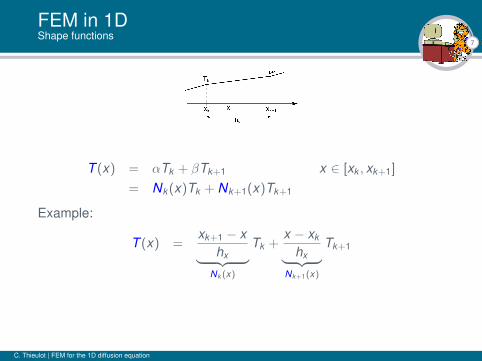
FEM in 1DShape functions
T (x) = αTk + βTk+1 x ∈ [xk , xk+1]
= Nk (x)Tk + Nk+1(x)Tk+1
Example:
T (x) =xk+1 − x
hx︸ ︷︷ ︸Nk (x)
Tk +x − xk
hx︸ ︷︷ ︸Nk+1(x)
Tk+1
I x = xk yields T (xk ) = TkI x = xk+1 yields T (xk+1) = Tk+1I x = x1/2 = (xk + xk+1)/2 yields T (x1/2) = (Tk + Tk+1)/2
C. Thieulot | FEM for the 1D diffusion equation

7
FEM in 1DShape functions
T (x) = αTk + βTk+1 x ∈ [xk , xk+1]
= Nk (x)Tk + Nk+1(x)Tk+1
Example:
T (x) =xk+1 − x
hx︸ ︷︷ ︸Nk (x)
Tk +x − xk
hx︸ ︷︷ ︸Nk+1(x)
Tk+1
I x = xk yields T (xk ) = TkI x = xk+1 yields T (xk+1) = Tk+1I x = x1/2 = (xk + xk+1)/2 yields T (x1/2) = (Tk + Tk+1)/2
C. Thieulot | FEM for the 1D diffusion equation

8
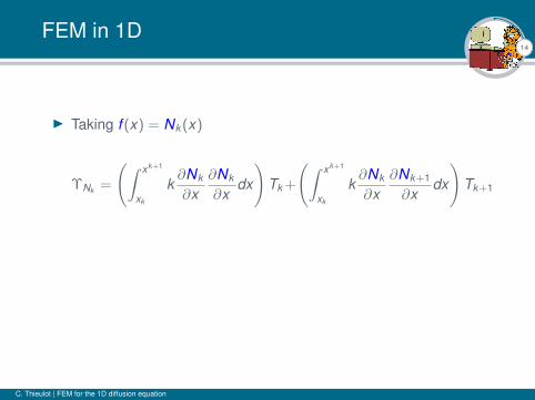
FEM in 1D.
Let us go back to
∑elts
∫
Ωe
f (x)ρCp∂T∂t
dx︸ ︷︷ ︸Λe
f
+
∫Ωe
∂f∂x
k∂T∂x
dx︸ ︷︷ ︸Υe
f
= 0
and compute Λef and Υe
f separately.
C. Thieulot | FEM for the 1D diffusion equation

9
FEM in 1D.
Λef =
∫ xk+1
xk
f (x)ρCpT (x)dx
=
∫ xk+1
xk
f (x)ρCp [Nk (x)Tk + Nk+1(x)Tk+1] dx
=
∫ xk+1
xk
f (x)ρCpNk (x)Tk dx +
∫ xk+1
xk
f (x)ρCpNk+1(x)Tk+1dx
=
(∫ xk+1
xk
f (x)ρCpNk (x)dx)
Tk +
(∫ xk+1
xk
f (x)ρCpNk+1(x)dx)
Tk+1
C. Thieulot | FEM for the 1D diffusion equation

10
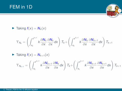
FEM in 1D.
I Taking f (x) = Nk (x) and omitting ’(x)’ in the rhs:
ΛNk =
(∫ xk+1
xk
ρCpNk Nk dx)
Tk +
(∫ xk+1
xk
ρCpNk Nk+1dx)
Tk+1
I Taking f (x) = Nk+1(x) and omitting ’(x)’ in the rhs:
ΛNk+1 =
(∫ xk+1
xk
ρCpNk+1Nk dx)
Tk +
(∫ xk+1
xk
ρCpNk+1Nk+1dx)
Tk+1
C. Thieulot | FEM for the 1D diffusion equation

10
FEM in 1D.
I Taking f (x) = Nk (x) and omitting ’(x)’ in the rhs:
ΛNk =
(∫ xk+1
xk
ρCpNk Nk dx)
Tk +
(∫ xk+1
xk
ρCpNk Nk+1dx)
Tk+1
I Taking f (x) = Nk+1(x) and omitting ’(x)’ in the rhs:
ΛNk+1 =
(∫ xk+1
xk
ρCpNk+1Nk dx)
Tk +
(∫ xk+1
xk
ρCpNk+1Nk+1dx)
Tk+1
C. Thieulot | FEM for the 1D diffusion equation

11
FEM in 1D.
ΛNk
ΛNk+1
=
∫ xk+1
xkNkρCpNk dx
∫ xk+1
xkNkρCpNk+1dx∫ xk+1
xkNk+1ρCpNk dx
∫ xk+1
xkNk+1ρCpNk+1dx
· Tk
Tk+1
or,
ΛNk
ΛNk+1
=
∫ xk+1
xk
ρCp
Nk Nk Nk Nk+1
Nk+1Nk Nk+1Nk+1
dx
· Tk
Tk+1
C. Thieulot | FEM for the 1D diffusion equation

11
FEM in 1D.
ΛNk
ΛNk+1
=
∫ xk+1
xkNkρCpNk dx
∫ xk+1
xkNkρCpNk+1dx∫ xk+1
xkNk+1ρCpNk dx
∫ xk+1
xkNk+1ρCpNk+1dx
· Tk
Tk+1
or, ΛNk
ΛNk+1
=
∫ xk+1
xk
ρCp
Nk Nk Nk Nk+1
Nk+1Nk Nk+1Nk+1
dx
· Tk
Tk+1
C. Thieulot | FEM for the 1D diffusion equation

12
FEM in 1D.
Finally, we can define the vectors
~NT =
Nk (x)
Nk+1(x)
and
~T e =
Tk
Tk+1
~T e =
Tk
Tk+1
so that ΛNk
ΛNk+1
=
(∫ xk+1
xk
~NTρCp~Ndx)· ~T e
C. Thieulot | FEM for the 1D diffusion equation

13
FEM in 1D
Back to the diffusion term:
Υef =
∫ xk+1
xk
∂f∂x
k∂T∂x
dx
=
∫ xk+1
xk
∂f∂x
k∂(Nk (x)Tk + Nk+1(x)Tk+1)
∂xdx
=
(∫ xk+1
xk
∂f∂x
k∂Nk
∂xdx
)Tk +
(∫ xk+1
xk
∂f∂x
k∂Nk+1
∂xdx
)Tk+1
C. Thieulot | FEM for the 1D diffusion equation
14
FEM in 1D
I Taking f (x) = Nk (x)
ΥNk =
(∫ xk+1
xk
k∂Nk
∂x∂Nk
∂xdx
)Tk +
(∫ xk+1
xk
k∂Nk
∂x∂Nk+1
∂xdx
)Tk+1
I Taking f (x) = Nk+1(x)
ΥNk+1 =
(∫ xk+1
xk
k∂Nk+1
∂x∂Nk
∂xdx
)Tk +
(∫ xk+1
xk
k∂Nk+1
∂x∂Nk+1
∂xdx
)Tk+1
C. Thieulot | FEM for the 1D diffusion equation
14
FEM in 1D
I Taking f (x) = Nk (x)
ΥNk =
(∫ xk+1
xk
k∂Nk
∂x∂Nk
∂xdx
)Tk +
(∫ xk+1
xk
k∂Nk
∂x∂Nk+1
∂xdx
)Tk+1
I Taking f (x) = Nk+1(x)
ΥNk+1 =
(∫ xk+1
xk
k∂Nk+1
∂x∂Nk
∂xdx
)Tk +
(∫ xk+1
xk
k∂Nk+1
∂x∂Nk+1
∂xdx
)Tk+1
C. Thieulot | FEM for the 1D diffusion equation

15
FEM in 1D
ΥNk
ΥNk+1
=
∫ xk+1
xk
∂Nk∂x k ∂Nk
∂x dx∫ xk+1
xk
∂Nk∂x k ∂Nk+1
∂x dx
∫ xk+1
xk
∂Nk+1∂x k ∂Nk
∂x dx∫ xk+1
xk
∂Nk+1∂x k ∂Nk+1
∂x dx
· Tk
Tk+1
or, ΥNk
ΥNk+1
=
∫ xk+1
xk
k
∂Nk∂x
∂Nk∂x
∂Nk∂x
∂Nk+1∂x
∂Nk+1∂x
∂Nk∂x
∂Nk+1∂x
∂Nk+1∂x
dx
· Tk
Tk+1
C. Thieulot | FEM for the 1D diffusion equation

15
FEM in 1D
ΥNk
ΥNk+1
=
∫ xk+1
xk
∂Nk∂x k ∂Nk
∂x dx∫ xk+1
xk
∂Nk∂x k ∂Nk+1
∂x dx
∫ xk+1
xk
∂Nk+1∂x k ∂Nk
∂x dx∫ xk+1
xk
∂Nk+1∂x k ∂Nk+1
∂x dx
· Tk
Tk+1
or, ΥNk
ΥNk+1
=
∫ xk+1
xk
k
∂Nk∂x
∂Nk∂x
∂Nk∂x
∂Nk+1∂x
∂Nk+1∂x
∂Nk∂x
∂Nk+1∂x
∂Nk+1∂x
dx
· Tk
Tk+1
C. Thieulot | FEM for the 1D diffusion equation

16
FEM in 1D
Finally, we can define the vector
~BT =
∂Nk∂x
∂Nk+1∂x
so that ΥNk
ΥNk+1
=
(∫ xk+1
xk
~BT k~Bdx)· ~T e
C. Thieulot | FEM for the 1D diffusion equation
17
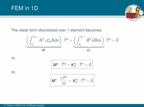
FEM in 1D
The weak form discretised over 1 element becomes(∫ xk+1
xk
~NTρCp~Ndx)
︸ ︷︷ ︸Me
·~T e +
(∫ xk+1
xk
~BT k~Bdx)
︸ ︷︷ ︸K e
d
·~T e = ~0
or,
Me · ~T e + K ed · ~T e = ~0
or,
Me · ∂~T e
∂t+ K e
d · ~T e = ~0
C. Thieulot | FEM for the 1D diffusion equation

18
FEM in 1D
Thieulot, PEPI 188, 2011
C. Thieulot | FEM for the 1D diffusion equation
19
FEM in 1D
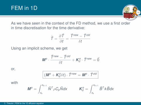
As we have seen in the context of the FD method, we use a first orderin time discretisation for the time derivative:
~T =∂~T∂t
=~T new − ~T old
δt
Using an implicit scheme, we get
Me ·~T new − ~T old
δt+ K e
d · ~T new = ~0
or,
(Me + K ed δt) · ~T new = Me · ~T old
with
Me =
∫ xk+1
xk
~NTρCp~Ndx K ed =
∫ xk+1
xk
~BT k~Bdx
C. Thieulot | FEM for the 1D diffusion equation

20
FEM in 1D
Let us compute M for an element:
Me =
∫ xk+1
xk
~NTρCp~Ndx
with
~NT =
Nk (x)
Nk+1(x)
=
xk+1−xhx
x−xkhx
Then
Me =
(M11 M12M21 M22
)=
∫ xk+1
xkρCpNk Nk dx
∫ xk+1
xkρCpNk Nk+1dx∫ xk+1
xkρCpNk+1Nk dx
∫ xk+1
xkρCpNk+1Nk+1dx
I need to compute 3 integrals (M12 = M21)
C. Thieulot | FEM for the 1D diffusion equation

21
FEM in 1D
Let us look at M11:
M11 =
∫ xk+1
xk
ρCpNk (x)Nk (x)dx =
∫ xk+1
xk
ρCpxk+1 − x
hx
xk+1 − xhx
dx
It is customary to carry out a change of variables (mapping x → r ):
r =2hx
(x − xk )− 1 x =hx
2(1 + r) + xk
C. Thieulot | FEM for the 1D diffusion equation

22
FEM in 1D
In what follows we assume for simplicity that ρ and Cp are constantwithin each element.
M11 = ρCp
∫ xk+1
xk
xk+1 − xhx
xk+1 − xhx
dx =ρCphx
8
∫ +1
−1(1−r)(1−r)dr =
hx
3ρCp
Similarly we arrive at
M12 = ρCp
∫ xk+1
xk
xk+1 − xhx
x − xk
hxdx =
ρCphx
8
∫ +1
−1(1− r)(1 + r)dr =
hx
6ρCp
and
M22 = ρCp
∫ xk+1
xk
x − xk
hx
x − xk
hxdx =
ρCphx
8
∫ +1
−1(1+r)(1+r)dr =
hx
3ρCp
C. Thieulot | FEM for the 1D diffusion equation

23
FEM in 1D
Finally
Me =hx
3ρCp
(1 1/2
1/2 1
)
C. Thieulot | FEM for the 1D diffusion equation

24
FEM in 1D
In the new coordinate system, the shape functions
Nk (x) =xk+1 − x
hxNk+1(x) =
x − xk
hx
becomeNk (r) =
12
(1− r) Nk+1(r) =12
(1 + r)
Also,∂Nk
∂x= − 1
hx
∂Nk+1
∂x=
1hx
so that
~BT =
∂Nk∂x
∂Nk+1∂x
=
− 1hx
1hx
C. Thieulot | FEM for the 1D diffusion equation

24
FEM in 1D
In the new coordinate system, the shape functions
Nk (x) =xk+1 − x
hxNk+1(x) =
x − xk
hx
becomeNk (r) =
12
(1− r) Nk+1(r) =12
(1 + r)
Also,∂Nk
∂x= − 1
hx
∂Nk+1
∂x=
1hx
so that
~BT =
∂Nk∂x
∂Nk+1∂x
=
− 1hx
1hx
C. Thieulot | FEM for the 1D diffusion equation

25
FEM in 1D
We here also assume that k is constant within the element:
Kd =
∫ xk+1
xk
~BT k~Bdx = k∫ xk+1
xk
~BT ~Bdx
simply becomes
Kd = k∫ xk+1
xk
1h2
x
(1 −1−1 1
)dx
and then
Kd =khx
(1 −1−1 1
)
C. Thieulot | FEM for the 1D diffusion equation

25
FEM in 1D
We here also assume that k is constant within the element:
Kd =
∫ xk+1
xk
~BT k~Bdx = k∫ xk+1
xk
~BT ~Bdx
simply becomes
Kd = k∫ xk+1
xk
1h2
x
(1 −1−1 1
)dx
and then
Kd =khx
(1 −1−1 1
)
C. Thieulot | FEM for the 1D diffusion equation

26
FEM in 1D
For each element
(Me + K ed δt)︸ ︷︷ ︸
Ae
·~T new = Me · ~T old︸ ︷︷ ︸~be
or,Ae · ~T new = ~be
C. Thieulot | FEM for the 1D diffusion equation

26
FEM in 1D
For each element
(Me + K ed δt)︸ ︷︷ ︸
Ae
·~T new = Me · ~T old︸ ︷︷ ︸~be
or,Ae · ~T new = ~be
C. Thieulot | FEM for the 1D diffusion equation

27
FEM in 1D
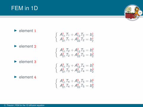
I element 1
A1 ·(
T1T2
)= b1
I element 2
A2 ·(
T2T3
)= b2
I element 3
A3 ·(
T3T4
)= b3
I element 4
A4 ·(
T4T5
)= b4
C. Thieulot | FEM for the 1D diffusion equation
28
FEM in 1D
I element 1 A1
11T1 + A112T2 = b1
xA1
21T1 + A122T2 = b1
y
I element 2 A2
11T2 + A212T3 = b2
1A2
21T2 + A222T3 = b2
2
I element 3 A3
11T3 + A312T4 = b3
1A3
21T3 + A322T4 = b3
2
I element 4 A4
11T4 + A412T5 = b4
1A4
21T4 + A422T5 = b4
2
C. Thieulot | FEM for the 1D diffusion equation

29
FEM in 1D
All equations can be cast into a single linear system: this is theassembly phase.
A111 A1
12
A121 A1
22+A211 A2
12
A221 A2
22+A311 A3
12
A321 A3
22+A411 A4
12
A421 A4
22
T1
T2
T3
T4
T5
=
b11
b12 + b2
1
b22 + b3
1
b32 + b4
1
b42
C. Thieulot | FEM for the 1D diffusion equation

30
FEM in 1D
C. Thieulot | FEM for the 1D diffusion equation
31
FEM in 1D
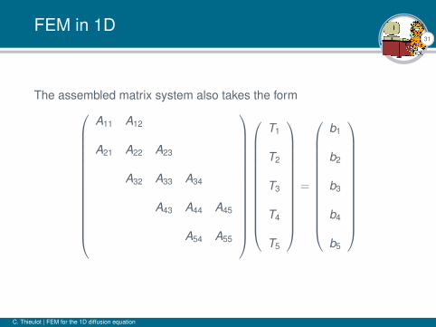
The assembled matrix system also takes the form
A11 A12
A21 A22 A23
A32 A33 A34
A43 A44 A45
A54 A55
T1
T2
T3
T4
T5
=
b1
b2
b3
b4
b5
C. Thieulot | FEM for the 1D diffusion equation

32
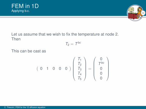
FEM in 1DApplying b.c.
Let us assume that we wish to fix the temperature at node 2.
ThenT2 = T bc
This can be cast as
(0 1 0 0 0
)
T1T2T3T4T5
=
0
T bc
000
C. Thieulot | FEM for the 1D diffusion equation

32
FEM in 1DApplying b.c.
Let us assume that we wish to fix the temperature at node 2.Then
T2 = T bc
This can be cast as
(0 1 0 0 0
)
T1T2T3T4T5
=
0
T bc
000
C. Thieulot | FEM for the 1D diffusion equation
32
FEM in 1DApplying b.c.
Let us assume that we wish to fix the temperature at node 2.Then
T2 = T bc
This can be cast as
(0 1 0 0 0
)
T1T2T3T4T5
=
0
T bc
000
C. Thieulot | FEM for the 1D diffusion equation

33
FEM in 1DApplying b.c.
This replaces the second line in the previous matrix equation:
A11 A12
0 1 0
A32 A33 A34
A43 A44 A45
A54 A55
T1
T2
T3
T4
T5
=
b1
T bc
b3
b4
b5
C. Thieulot | FEM for the 1D diffusion equation

34
FEM in 1DApplying b.c.
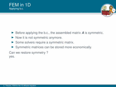
I Before applying the b.c., the assembled matrix A is symmetric.
I Now it is not symmetric anymore.I Some solvers require a symmetric matrix.I Symmetric matrices can be stored more economically.
Can we restore symmetry ?yes.duh :)
C. Thieulot | FEM for the 1D diffusion equation

34
FEM in 1DApplying b.c.
I Before applying the b.c., the assembled matrix A is symmetric.I Now it is not symmetric anymore.
I Some solvers require a symmetric matrix.I Symmetric matrices can be stored more economically.
Can we restore symmetry ?yes.duh :)
C. Thieulot | FEM for the 1D diffusion equation

34
FEM in 1DApplying b.c.
I Before applying the b.c., the assembled matrix A is symmetric.I Now it is not symmetric anymore.I Some solvers require a symmetric matrix.
I Symmetric matrices can be stored more economically.
Can we restore symmetry ?yes.duh :)
C. Thieulot | FEM for the 1D diffusion equation

34
FEM in 1DApplying b.c.
I Before applying the b.c., the assembled matrix A is symmetric.I Now it is not symmetric anymore.I Some solvers require a symmetric matrix.I Symmetric matrices can be stored more economically.
Can we restore symmetry ?
yes.duh :)
C. Thieulot | FEM for the 1D diffusion equation
34
FEM in 1DApplying b.c.
I Before applying the b.c., the assembled matrix A is symmetric.I Now it is not symmetric anymore.I Some solvers require a symmetric matrix.I Symmetric matrices can be stored more economically.
Can we restore symmetry ?yes.
duh :)
C. Thieulot | FEM for the 1D diffusion equation

34
FEM in 1DApplying b.c.
I Before applying the b.c., the assembled matrix A is symmetric.I Now it is not symmetric anymore.I Some solvers require a symmetric matrix.I Symmetric matrices can be stored more economically.
Can we restore symmetry ?yes.duh :)
C. Thieulot | FEM for the 1D diffusion equation
35
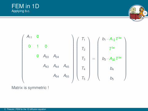
FEM in 1DApplying b.c.
A11 0
0 1 0
0 A33 A34
A43 A44 A45
A54 A55
T1
T2
T3
T4
T5
=
b1−A12T bc
T bc
b3−A32T bc
b4
b5
Matrix is symmetric !
C. Thieulot | FEM for the 1D diffusion equation

36
FEM in 1DApplying b.c.
The matrix is now symmetric, but its condition number may have beenchanged.
Fix:
A11 0
0 A22 0
0 A33 A34
A43 A44 A45
A54 A55
T1
T2
T3
T4
T5
=
b1−A12T bc
A22T bc
b3−A32T bc
b4
b5
C. Thieulot | FEM for the 1D diffusion equation

36
FEM in 1DApplying b.c.
The matrix is now symmetric, but its condition number may have beenchanged.Fix:
A11 0
0 A22 0
0 A33 A34
A43 A44 A45
A54 A55
T1
T2
T3
T4
T5
=
b1−A12T bc
A22T bc
b3−A32T bc
b4
b5
C. Thieulot | FEM for the 1D diffusion equation

37
FEM in 1DProgram structure
C. Thieulot | FEM for the 1D diffusion equation

38
FEM in 1DExercise
The initial temperature profile is as follows:
T (x , t = 0) = 200 x < Lx/2 T (x , t = 0) = 100 x ≥ Lx/2
C. Thieulot | FEM for the 1D diffusion equation

39
Exercise
The properties of the material are as follows:
ρ = 3000 k = 3 Cp = 1000
Furthermore, Lx = 100km.Boundary conditions are:
T (t , x = 0) = 200C T (t , x = Lx ) = 100C
There are nelx elements and nnx nodes. All elements are hx long.The code will carry out nstep timesteps of length dt.
C. Thieulot | FEM for the 1D diffusion equation

40
Exercise
C. Thieulot | FEM for the 1D diffusion equation

41
Exercise
C. Thieulot | FEM for the 1D diffusion equation

42
FEM in 1DMesh connectivity
I Typically one uses a connectivity arrayI Two-dimensional integer arrayI icon ( # elements , # vertices per element )
C. Thieulot | FEM for the 1D diffusion equation

43
FEM in 1DMesh connectivity
Example
I The above mesh counts 5 elements.I Each element is composed of 2 nodes
icon(1,1)=1icon(1,2)=2icon(2,1)=2icon(2,2)=3icon(3,1)=3icon(3,2)=4icon(4,1)=4icon(4,2)=5icon(5,1)=5icon(5,2)=6
C. Thieulot | FEM for the 1D diffusion equation

44
FEM in 1D
I The above mesh counts 10 elements.I Each element is composed of 3 nodes
C. Thieulot | FEM for the 1D diffusion equation

45
FEM in 1DProgram structure
C. Thieulot | FEM for the 1D diffusion equation

46
FEM in 1DMeshing
C. Thieulot | FEM for the 1D diffusion equation

47
FEM in 1D
C. Thieulot | FEM for the 1D diffusion equation

48
FEM in 1D
C. Thieulot | FEM for the 1D diffusion equation