computational medicine in data mining and modeling || particle dynamics and design of nano-drug...

Chapter 8

Particle Dynamics and Design of Nano-drug

Delivery Systems

Tijana Djukic

8.1 Introduction

Particles have been increasingly investigated in recent years as “smart” delivery

systems, which can be applied in biomedical imaging, but also as therapeutical

agents in cardiovascular and oncological treatments [1–3]. Such drug delivery

systems consist of nanoparticles that can be loaded with contrast agents or drug

molecules (monoclonal antibodies (mAbs) or small-molecule agents). Particles are

sufficiently small to be injected at the systemic level and transported through the

circulatory system to various organs and body districts. The size of particles ranges

from few tens of nanometers to hundreds of nanometers [4, 5] to few microns

[6]. Also, they can have various shapes, including spherical, spheroidal [7], or other

more complex shapes [8]. The majority are made by polymeric or lipid materials,

but can also be made of silica, gold, or iron oxide.

There are two strategies currently considered in the field of delivery of

nanoparticles to solid tumors. The strategy that has been traditionally considered

is the passive strategy, based on the enhanced permeability and retention effect

(EPR) [9] – nanoparticles that extravasate through fenestrations found in the tumor

vasculature are entrapped in the extracellular matrix and transported from the

vascular compartment to the inner region of the tumor mass. As an alternative to

the passive strategy, an active delivery strategy, which is gaining more and more

interest recently, is based on the targeting of the tumor vasculature through ligand-

receptor specific interactions. In this case particles are designed to be able to sense

the difference between normal and tumor endothelium and “search” for biological

and biophysical specificities such as overexpression of disease-specific receptor

molecules [10] or the appearance of abnormally large inter- or intra-endothelial

gaps [11]. In vascular targeting, nanoparticles should be able to attach to a specific

T. Djukic (*)

Faculty of Engineering, R&D Center for Bioengineering, Kragujevac, Serbia

e-mail: [email protected]

G. Rakocevic et al. (eds.), Computational Medicine in Data Mining and Modeling,DOI 10.1007/978-1-4614-8785-2_8, © Springer Science+Business Media New York 2013

309

mailto:[email protected]

part of a blood vessel and release their payload, i.e., drug molecules or smaller

particulate formulations specifically designed for further transport through the

tumor mass.

In this type of drug delivery systems, it is very important to achieve particle

margination, i.e., the capability to move towards the endothelium and sense the

mentioned biological and biophysical diversities. An effective way to stimulate

particle margination could be the control of their size, shape, and density [12].

In microcirculation, in proximity to the walls of small vessels, the flow is mainly

governed by viscous forces. If there is no effect of gravitational or magnetic forces,

light spherical particles tend to move parallel to the walls without crossing the

streamlines [13, 14]. On the other hand, heavy particles, made of silica, gold, or iron

oxide, would drift laterally under the influence of gravity [15]. However, nonspher-

ical particles have a more complicated behavior. Hence, the conclusion was made

that both wall proximity and particle inertia have a dramatic influence on particle

dynamics [16, 17].

Numerical modeling of particle motion is important since it can facilitate the

analysis of influence of various parameters relevant in design of nanoparticles, such

as size, shape, and surface characteristics. Finite element method enables the

development of adequate particle tracking models. But this method requires very

fine meshes and very small time step to obtain precise simulation results. On the

other hand, discrete particle methods are suitable since they can provide a more

detailed analysis of particle trajectories and interaction forces between fluid and

particles, as well as among the particles themselves. One of these discrete methods

is the lattice Boltzmann method, which is considered in this chapter.

This chapter is organized as follows: in Sect. 8.2 the basics of lattice Boltzmann

method are explained, including theoretical background and implementation

details, such as discretization procedure and definition of boundary conditions.

Section 8.3 explains the model that was used for simulations of solid–fluid interac-

tion. Examples and results of simulations are the subject of Sect. 8.4. Section 8.5

concludes the chapter.

8.2 Lattice Boltzmann Method

Lattice Boltzmannmethod belongs to the class of problems named Cellular Automata

(CA). Thismeans that the physical system can be observed in an idealizedway, so that

space and time are discretized, and the whole domain is made up of a large number of

identical cells [18]. Special form of CA, the so-called lattice gas automata (LGA)

[19], describes the dynamics of particles that move and collide in discrete time-space

domain. The advantages of this method are simple implementation, the stability of the

solution, easy assignment of boundary conditions, and natural parallelization. How-

ever, this method has many drawbacks, like statistical error, special averaging

procedures necessary to obtain macroscopic quantities, and others. In order to remove

the aforementioned disadvantages of LGA, the new improved method was developed

that can simplify the simulations of fluid flow. This method is lattice Boltzmann

310 T. Djukic

(LB) method. The main goal during the development of the new LB method was to

create a new improved model that can simplify the simulations of fluid flow. Using

LB method, with certain limitations, it is possible to obtain the solution of

Navier–Stokes equation, which means that it can be used to simulate fluid flow.

Special propagation function is defined, so that it depends on the state of neighboring

cells and it has an identical form for all cells. The state of all cells is updated

synchronously, through a series of iterations, in discrete time steps. This way a greater

numerical accuracy and efficiency is obtained in LB method.

8.2.1 Theoretical Background

The Boltzmann equation is a partial differential equation that describes the behavior

and movement of particles in space and is valid for continuum. The basic quantity

in Boltzmann equation is single distribution function f. The distribution function is

defined in such a way that f(x,v,t) represents the probability for particles to be

located within a space element dx dv around position (x,v), at time t, where x and vare the spatial position vector and the particle velocity vector, respectively.

In the presence of an external force field g, distribution function balance

equation – Boltzmann equation – has the following form:

∂f∂t

þ v∂f∂x

þ g

m� ∂f∂v

¼ Ω (8.1)

where Ω is the collision integral or the collision operator, and it represents the

changes in the distribution function due to the interparticle collisions.

The collision operatorΩ is quadratic in f and is represented using a very complex

expression. Hence, a simplified model is introduced, initially proposed by

Bhatnagar, Gross, and Krook [20]. An assumption is made that the effect of the

collision between particles is to drive the fluid towards a local equilibrium state.

This model is known as the single relaxation time approximation or the Bhatnagar-

Gross-Krook (BGK) model. Operator Ω is defined as follows:

Ω ¼ � 1

τf � f 0ð Þ� �

(8.2)

where τ is the relaxation time (the average time period between two collisions) and

f (0) is the equilibrium distribution function, the so-called Maxwell-Boltzmann

distribution function, which is given by:

f 0ð Þ x; v; tð Þ ¼ ρ x; tð Þ2πθ x; tð Þð ÞD=2

exp � u x; tð Þ � vð Þ22θ x; tð Þ

!(8.3)

In this expression D is the number of physical dimensions (D ¼ 3 for three-

dimensional domain); θ ¼ kBT/m; kB ¼ 1, 38 � 10�23 JK is the Boltzmann constant;

8 Particle Dynamics and Design of Nano-drug Delivery Systems 311

T is the absolute temperature, expressed in Kelvins (K); m is the particle mass

(in the sequel, it is assumed that the mass of a single particle is m ¼ 1).

Finally, BGK model of the continuous Boltzmann equation is given by:

∂f∂t

þ v∂f∂x

þ g∂f∂v

¼ � 1

τf � f 0ð Þ� �

(8.4)

If Eq. (8.4) is transformed according to the procedure described in [21, 22], the

familiar Navier–Stokes equation for the incompressible fluid is obtained:

∂ρ∂t

þ ∂∂x

ρuð Þ ¼ 0 (8.5)

ρdu

dtþ ∂∂x

pI� 2μSSð Þ ¼ ρg (8.6)

where S is the strain rate tensor and pressure p in LB method is introduced into the

system of equations through the ideal gas law:

p ¼ ρθ ¼ ρkBT

m(8.7)

In LB simulations there are two important approximations that need to be taken

into account. First some new quantities have to be introduced. The characteristic

length of the observed domain is denoted with L, and cs denotes the characteristicspeed of particles, which is also often called speed of sound in lattice units. This

characteristic speed can be expressed as:

cs �ffiffiffiffiffiffiffiffiffikB

T

m

r¼

ffiffiffiθ

p(8.8)

Mean free path (the average path of a particle between two collisions) is denoted

with l ¼ csτ. Knudsen number is defined as the ratio between mean free path and

characteristic lengthscale of the considered system:

Kn ¼ l

L(8.9)

The entire approach and BGK model are valid only in the limit of small Knudsen

number.

The Mach number is defined as the ratio between the characteristic fluid velocity

and the “speed of sound” cs:

Ma ¼ uj jcs

(8.10)

During the derivation procedure higher order members in some expressions are

neglected, due to the introduction of an approximation that LB simulations are

312 T. Djukic

performed in the limit of small Mach number. This needs to be taken into account

when defining the characteristic fluid velocity in simulations.

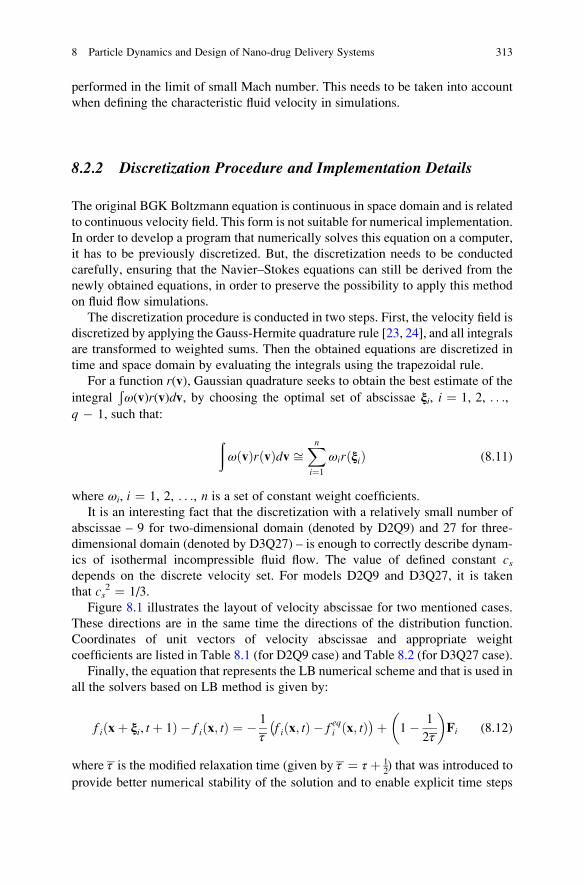
8.2.2 Discretization Procedure and Implementation Details

The original BGK Boltzmann equation is continuous in space domain and is related

to continuous velocity field. This form is not suitable for numerical implementation.

In order to develop a program that numerically solves this equation on a computer,

it has to be previously discretized. But, the discretization needs to be conducted

carefully, ensuring that the Navier–Stokes equations can still be derived from the

newly obtained equations, in order to preserve the possibility to apply this method

on fluid flow simulations.

The discretization procedure is conducted in two steps. First, the velocity field is

discretized by applying the Gauss-Hermite quadrature rule [23, 24], and all integrals

are transformed to weighted sums. Then the obtained equations are discretized in

time and space domain by evaluating the integrals using the trapezoidal rule.

For a function r(v), Gaussian quadrature seeks to obtain the best estimate of the

integralÐω(v)r(v)dv, by choosing the optimal set of abscissae ξi, i ¼ 1, 2, . . .,

q � 1, such that:

ðω vð Þr vð Þdv ffi

Xni¼1

ωir ξið Þ (8.11)

where ωi, i ¼ 1, 2, . . ., n is a set of constant weight coefficients.

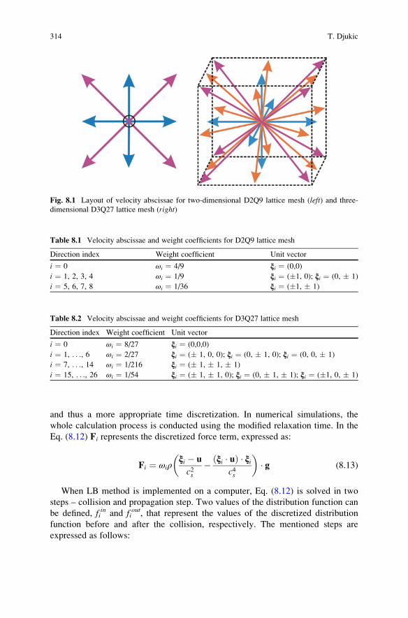
It is an interesting fact that the discretization with a relatively small number of

abscissae – 9 for two-dimensional domain (denoted by D2Q9) and 27 for three-

dimensional domain (denoted by D3Q27) – is enough to correctly describe dynam-

ics of isothermal incompressible fluid flow. The value of defined constant csdepends on the discrete velocity set. For models D2Q9 and D3Q27, it is taken

that cs2 ¼ 1/3.

Figure 8.1 illustrates the layout of velocity abscissae for two mentioned cases.

These directions are in the same time the directions of the distribution function.

Coordinates of unit vectors of velocity abscissae and appropriate weight

coefficients are listed in Table 8.1 (for D2Q9 case) and Table 8.2 (for D3Q27 case).

Finally, the equation that represents the LB numerical scheme and that is used in

all the solvers based on LB method is given by:

f i xþ ξi, tþ 1ð Þ � f i x; tð Þ ¼ � 1

τf i x; tð Þ � f eqi x; tð Þ� �þ 1� 1

2τ

� �Fi (8.12)

where τ is the modified relaxation time (given by τ ¼ τ þ 12) that was introduced to

provide better numerical stability of the solution and to enable explicit time steps


and thus a more appropriate time discretization. In numerical simulations, the

whole calculation process is conducted using the modified relaxation time. In the

Eq. (8.12) Fi represents the discretized force term, expressed as:

Fi ¼ ωiρξi � u

c2s� ξi � uð Þ � ξi

c4s

� �� g (8.13)

When LB method is implemented on a computer, Eq. (8.12) is solved in two

steps – collision and propagation step. Two values of the distribution function can

be defined, fiin and fi

out, that represent the values of the discretized distribution

function before and after the collision, respectively. The mentioned steps are

expressed as follows:

Fig. 8.1 Layout of velocity abscissae for two-dimensional D2Q9 lattice mesh (left) and three-

dimensional D3Q27 lattice mesh (right)

Table 8.1 Velocity abscissae and weight coefficients for D2Q9 lattice mesh

Direction index Weight coefficient Unit vector

i ¼ 0 ωi ¼ 4/9 ξi ¼ (0,0)

i ¼ 1, 2, 3, 4 ωi ¼ 1/9 ξi ¼ (�1, 0); ξi ¼ (0, � 1)

i ¼ 5, 6, 7, 8 ωi ¼ 1/36 ξi ¼ (�1, � 1)

Table 8.2 Velocity abscissae and weight coefficients for D3Q27 lattice mesh

Direction index Weight coefficient Unit vector

i ¼ 0 ωi ¼ 8/27 ξi ¼ (0,0,0)

i ¼ 1, . . ., 6 ωi ¼ 2/27 ξi ¼ (� 1, 0, 0); ξi ¼ (0, � 1, 0); ξi ¼ (0, 0, � 1)

i ¼ 7, . . ., 14 ωi ¼ 1/216 ξi ¼ (� 1, � 1, � 1)

i ¼ 15, . . ., 26 ωi ¼ 1/54 ξi ¼ (� 1, � 1, 0); ξi ¼ (0, � 1, � 1); ξi ¼ (�1, 0, � 1)

314 T. Djukic

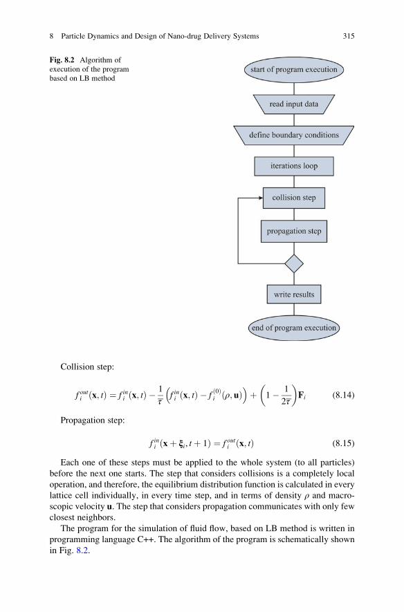
Collision step:

f outi x; tð Þ ¼ f ini x; tð Þ � 1

τf ini x; tð Þ � f

0ð Þi ρ; uð Þ

� �þ 1� 1

2τ

� �Fi (8.14)

Propagation step:

f ini xþ ξi, tþ 1ð Þ ¼ f outi x; tð Þ (8.15)

Each one of these steps must be applied to the whole system (to all particles)

before the next one starts. The step that considers collisions is a completely local

operation, and therefore, the equilibrium distribution function is calculated in every

lattice cell individually, in every time step, and in terms of density ρ and macro-

scopic velocity u. The step that considers propagation communicates with only few

closest neighbors.

The program for the simulation of fluid flow, based on LB method is written in

programming language C++. The algorithm of the program is schematically shown

in Fig. 8.2.

Fig. 8.2 Algorithm of

execution of the program

based on LB method


It is important to emphasize that there must exist a loop of iterations, since

the problem is solved in a large number of time steps, until the steady state is

reached. Within this loop two steps defined with Eqs. (8.14) and (8.15) are

carried out.

8.2.3 Definition of Macroscopic Quantities

LB method describes the fluid on a molecular level, and the characteristics of the

fluid from the continuum aspect are implicitly contained in the model. The basic

quantity determined in LB simulation (the distribution function) is used to calculate

the macroscopic quantities that describe the fluid flow. Density and velocity can be

evaluated by calculating the following integrals:

ρ x; tð Þ ¼ðv

f x; v; tð Þdv (8.16)

u x; tð Þ ¼ 1

ρ x; tð Þðv

f x; v; tð Þvdv (8.17)

The integration is carried out on the whole velocity space.

After discretization, fluid density and velocity can be calculated as weighted

sums over a finite number of discrete abscissae that were used to discretize the

space domain:

ρ ¼Xq�1

i¼0

f i (8.18)

u ¼ 1

ρ

Xq¼1

i¼0

ξif i ¼1

ρρu� ρg=2ð Þ (8.19)

From this equation it can be seen that the velocity that is calculated in terms of

distribution function in LB simulations does not represent the “physical velocity.”

In order to evaluate the physical velocity (which is one of the most important

characteristics of the flow observed on the macroscopic level), it is necessary to use

the following expression:

u ¼ u þ g

2(8.20)

This should be taken into consideration when analyzing the simulation results

and when developing solvers based on LB method.

316 T. Djukic

Dynamic viscosity in LB simulations (called “lattice viscosity”) is calculated as

follows:

μs ¼ c2sρ τ � 1

2

� �(8.21)

The equation that defines the relation between fluid pressure and fluid density is

given by:

p ¼ c2sρθ ¼ c2sρkBT

m(8.22)

Stress tensor can be calculated using expression:

P ¼ c2sρI�τ � 1

2

� �c4s

S (8.23)

8.2.4 Boundary Conditions

All previous derivations did not take into account the boundary conditions (BC).

Still, in order to obtain valid results and to correctly simulate fluid flow, it is

necessary to define the boundary conditions appropriately. Typical types of bound-

ary conditions (periodical, bounce-back, and predefined pressure and velocity

Dirichlet BC) that are used to set up simulations in examples section will be briefly

explained in the sequel of this chapter.

8.2.4.1 Periodical Boundary Condition

This is the simplest type of boundary condition. Practically, one can observe the

boundary as if the inlet and the outlet are joined together. In the practical imple-

mentation, this BC is implemented within the propagation step. For all the nodes

that are on the boundary of the domain, the components of the distribution function

that should propagate outside of the domain boundary are being “redirected” such

that these values are transferred to the nodes that are located on the other (opposite)

boundary of the domain.

8.2.4.2 Bounce-Back Boundary Condition

This boundary condition is very simple for implementation and that is one of the

reasons for its wide popularity. It is most commonly applied when solving problems

with complex boundaries, such as the flow through a porous media [25]. If a certain

node of the mesh is marked as a solid node, i.e., as an obstacle, the components of

the distribution function in this node are copied from the components with opposite

abscissae unit vectors.


However, bounce-back boundary condition has its drawbacks that are discussed

in literature [26, 27]. The main drawback is that in case of a wrong implementation,

some instabilities and the misbalance in the continuity equation may occur.

A detailed analysis showed that applying this BC the second-order accuracy is

achieved but only when the boundary between solid and fluid domain is located

between the nodes of the mesh [28]. If the solid–fluid boundary is made of straight

lines, then it is desirable to use this approach. But if complex geometries with

curved boundaries are considered or when solid is placed inside fluid domain and

solid–fluid interaction is simulated, it is more efficient to use a different approach,

such as immersed boundary method, which will be discussed in the next chapter.

8.2.4.3 Pressure and Velocity Boundary Conditions

When the boundary conditions are observed in general, after the propagation step,

those nodes that are on the domain boundary will contain certain information about

the distribution function that are incoming from the wall, i.e., that are nonphysical.

The main objective of the propagation is to transfer the information from one node

to its closest neighboring nodes. Therefore it is evident that this information for

boundary nodes should be obtained from a node inside the wall. Since the nodes

inside the wall are not simulated, missing distribution function components must be

recomputed using a different approach. Also it is necessary to keep in mind that the

entire concept of derivation of Navier–Stokes equations must be valid in the whole

system, i.e., in all nodes, including boundary nodes. The discussion about conserv-

ing the continuity equation can be found in literature [29].

When the simulations of fluid flow are performed, it is most common to define the

value of velocity and pressure (that is the so-called Dirichlet boundary condition) or

to define the derivatives of these quantities, i.e., the fluxes of certain quantities (that

is the so-called Neumann boundary condition). It should be noted that in LBmethod

the density is defined, instead of pressure, since these two quantities are related with

the equation of state (8.22). Using these macroscopic values, it is possible to

calculate the missing components of the distribution function coming from the wall.

There are several types of velocity and pressure BCs that were proposed in

literature – the boundary condition proposed by Inamuro et al. [27], the Zou/He

approach [30], the regularized method [31], and the finite difference method, based

on an idea of Skordos [32]. In this implementation of LB method, the regularized

boundary condition was used. It is assumed that the pressure or velocity is directly

prescribed, i.e., the Dirichlet boundary condition is considered. Of course, since

only one macroscopic quantity is predefined, the relation between two quantities –

velocity and pressure – is also determined according to literature [22, 30]. The

recalculation of the distribution function is performed, and afterwards both the

collision and propagation steps are performed on all lattice nodes, including

boundary nodes. It was only necessary to correct the unknown components that

were incoming from the nodes inside the wall. Obviously the implementation of

this boundary condition accurately recovers not only the velocity and density but

also the stress tensor.

318 T. Djukic

8.3 Modeling Solid–Fluid Interaction

There are certain types of problems that require the simulation of two or more

physical systems that are in interaction. One of them is in the field of fluid flow

simulation, and it is analyzed in this chapter – particles (regarded as solid bodies)

moving through a fluid domain. In this case an external force exerted from the fluid

is acting on the solid, causing solid movement or deformations and vice versa –

solid is having certain influence on the fluid flow. That practically means that solid

and fluid are forming a coupled mechanical system. In order to simulate a system

like this, it is necessary to simulate both domains simultaneously, i.e., to model

solid–fluid interaction. There are two approaches in modeling solid–fluid interac-

tion: loose and strong coupling. In loose coupling approach the solid and fluid

domains are solved separately, and all the necessary parameters obtained in one

solver are passed to the solver for the other domain. In strong coupling both

domains are simulated in the same time, like it were a single mechanical system.

For certain problems it is easier to use loose coupling, due to easier implementation.

However there are some drawbacks of this approach, like the problem of time

integration. Since the physical characteristics of solid and fluid are different, it is

not always possible to use the same time step for numerical solving. On the other

hand, strong coupling is more applicable when it is necessary to accurately and

precisely predict the movement of solid body inside fluid domain. But this approach

also has its drawbacks. The solver that simultaneously solves both domains is much

more complex and slower, which was expected considering the increased number

of equations in the system. Examples in this chapter were simulated using strong

coupling approach, and therefore, in the sequel of this section, theoretical basics of

this approach will be discussed.

The basic idea of full interaction approach is to solve the complete domain (both

fluid flow and particle motion) in every time step. This will provide that all

quantities (both for particles and fluid) are changing simultaneously. The approach

that was successfully applied for problems of particle movement through fluid

domain [33] is used here to simulate motion of nanoparticles together with fluid.

This method is called immersed boundary method (abbreviated IBM), and it was

first developed and presented by Peskin [34]. This method uses a fixed Cartesian

mesh to represent the fluid domain, so that the fluid mesh is composed of Eulerian

points. This description is in accordance with LB representation of fluid domain, so

it is evident that this approach can be easily applied if fluid flow is simulated using

LB method. As far as particles (solid bodies in general definition of IBM) are

concerned, IBM represents solid body as an isolated part of fluid, with a boundary

represented by a set of Lagrangian points. The basic idea is to treat the physical

boundary between two domains as deformable with high stiffness [35]. Fluid is

acting on the solid, i.e., on the boundary surface, through a force that tends to

deform the boundary. However, in the bounding area this deformation yields to a


force that tends to restore the boundary to its original shape. These two forces have

to be in equilibrium. Practically, using the law of action and reaction (Newton’s

third law), the force exerted from the fluid and acting on the solid is acting on the

fluid near the boundary too and is distributed through a discrete delta function.

The entire solid–fluid domain is solved using Navier–Stokes equations, with exter-

nal force term. There are several ways to determine this force representing the

interaction between solid and fluid. Some of them are direct forcing term [36],

enhanced version of direct forcing scheme [37], penalty formulation [33], momen-

tum exchange method [38], and calculation based on velocity correction [39]. The

latter is used in this study to simulate the full interaction between fluid and

nanoparticles.

The following quantities are defined: XBl (s,t) represent the coordinates of

Lagrangian boundary points; l ¼ 1, 2,.., m, where m is the number of boundary

points; F(s,t) is the boundary force density, exerted from the fluid, acting on the

immersed object; g(x,t) is the fluid external force density; and δ(x � XBl (s,t)) is a

Dirac delta function.

All quantities that are required to simulate solid–fluid interaction are calculated

using interpolation from the boundary points. Since different discretization of solid

and fluid domain is possible, the problem of interpolation with diverse

discretization has to be considered. This is solved such that for each boundary

point belonging to the solid, the influence of a greater number of points from the

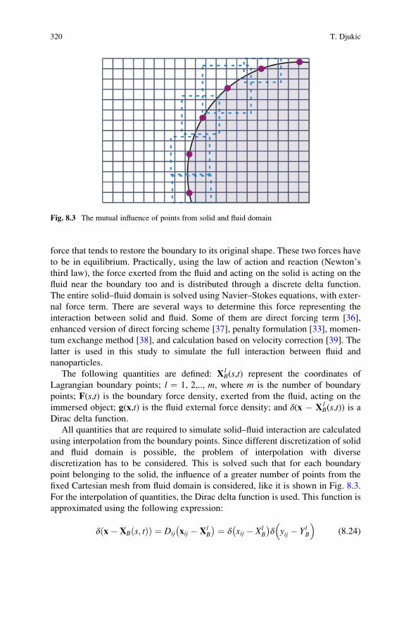
fixed Cartesian mesh from fluid domain is considered, like it is shown in Fig. 8.3.

For the interpolation of quantities, the Dirac delta function is used. This function is

approximated using the following expression:

δ x� XB s; tð Þð Þ ¼ Dij xij � XlB

� � ¼ δ xij � XlB

� �δ yij � Yl

B

� �(8.24)

Fig. 8.3 The mutual influence of points from solid and fluid domain

320 T. Djukic

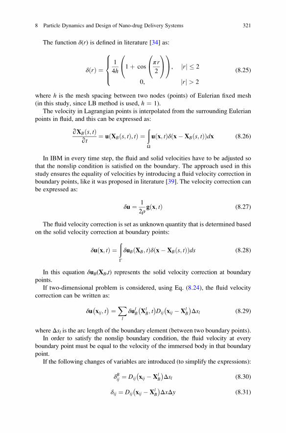
The function δ(r) is defined in literature [34] as:

δ rð Þ ¼1

4h1þ cos

π r

2

0@

1A

0@

1A, rj j � 2

0, rj j > 2

8>><>>:

(8.25)

where h is the mesh spacing between two nodes (points) of Eulerian fixed mesh

(in this study, since LB method is used, h ¼ 1).

The velocity in Lagrangian points is interpolated from the surrounding Eulerian

points in fluid, and this can be expressed as:

∂XB s; tð Þ∂t

¼ u XB s; tð Þ, tð Þ ¼ðΩ

u x; tð Þδ x� XB s; tð Þð Þdx (8.26)

In IBM in every time step, the fluid and solid velocities have to be adjusted so

that the nonslip condition is satisfied on the boundary. The approach used in this

study ensures the equality of velocities by introducing a fluid velocity correction in

boundary points, like it was proposed in literature [39]. The velocity correction can

be expressed as:

δu ¼ 1

2ρg x; tð Þ (8.27)

The fluid velocity correction is set as unknown quantity that is determined based

on the solid velocity correction at boundary points:

δu x; tð Þ ¼ðΓ

δuB XB; tð Þδ x� XB s; tð Þð Þds (8.28)

In this equation δuB(XB,t) represents the solid velocity correction at boundary

points.

If two-dimensional problem is considered, using Eq. (8.24), the fluid velocity

correction can be written as:

δu xij; t� � ¼X

l

δulB XlB; t

� �Dij xij � Xl

B

� �Δsl (8.29)

where Δsl is the arc length of the boundary element (between two boundary points).

In order to satisfy the nonslip boundary condition, the fluid velocity at every

boundary point must be equal to the velocity of the immersed body in that boundary

point.

If the following changes of variables are introduced (to simplify the expressions):

δBij ¼ Dij xij � XlB

� �Δsl (8.30)

δij ¼ Dij xij � XlB

� �ΔxΔy (8.31)


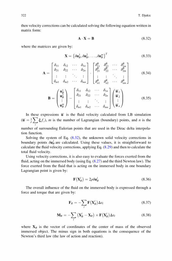
then velocity corrections can be calculated solving the following equation written in

matrix form:

A � X ¼ B (8.32)

where the matrices are given by:

X ¼ δu1B, δu2B, . . . , δu

mB

T(8.33)

A ¼δ11 δ12 � � � δ1nδ21 δ22 � � � δ2n

⋮ ⋮ . ..

⋮δm1 δm2 � � � δmn

26664

37775 �

δB11 δB12 � � � δB1mδB21 δB22 � � � δB2m

⋮ ⋮ . ..

⋮δBn1 δBn2 � � � δBnm

26664

37775 (8.34)

B ¼u1Bu2B⋮umB

0BB@

1CCA�

δ11 δ12 � � � δ1nδ21 δ22 � � � δ2n

⋮ ⋮ . ..

⋮δm1 δm2 � � � δmn

26664

37775

u 1

u 2

⋮u n

0BB@

1CCA (8.35)

In these expressions u is the fluid velocity calculated from LB simulation

(u ¼ 1ρ

Xi

ξi f i), m is the number of Lagrangian (boundary) points, аnd n is the

number of surrounding Eulerian points that are used in the Dirac delta interpola-

tion function.

Solving the system of Eq. (8.32), the unknown solid velocity corrections in

boundary points δuBl are calculated. Using these values, it is straightforward to

calculate the fluid velocity corrections, applying Eq. (8.29) and then to calculate the

total fluid velocity.

Using velocity corrections, it is also easy to evaluate the forces exerted from the

fluid, acting on the immersed body (using Eq. (8.27) and the third Newton law). The

force exerted from the fluid that is acting on the immersed body in one boundary

Lagrangian point is given by:

F XlB

� � ¼ 2ρδulB (8.36)

The overall influence of the fluid on the immersed body is expressed through a

force and torque that are given by:

FR ¼ �Xl

F XlB

� �Δsl (8.37)

MR ¼ �Xl

XlB � XR

� �� F XlB

� �Δsl (8.38)

where XR is the vector of coordinates of the center of mass of the observed

immersed object. The minus sign in both equations is the consequence of the

Newton’s third law (the law of action and reaction).

322 T. Djukic

If it is necessary to consider the influence of gravity force on the solid object,

another term is added in the expression for total force:

FR ¼ 1� ρfρp

!mG�

Xl

F XlB

� �Δsl (8.39)

Here m is the mass of solid object (particle), G is the gravity force acceleration,

and ρf and ρp are the fluid and particle density, respectively.

When force and torque acting on the particle are known, the equations of motion

can be written for the immersed body:

mdvCdt

¼ FR (8.40)

I0dωdt

¼ MR (8.41)

where m and I0 are the particle mass and moment of inertia, respectively, and vCand ω are the velocity and angular velocity of the particle, respectively.

Integrating these equations the position and orientation of particle are obtained.

Using this data the position of particle inside fluid domain is updated, and the entire

procedure is repeated until particle collides with one of the boundaries of the

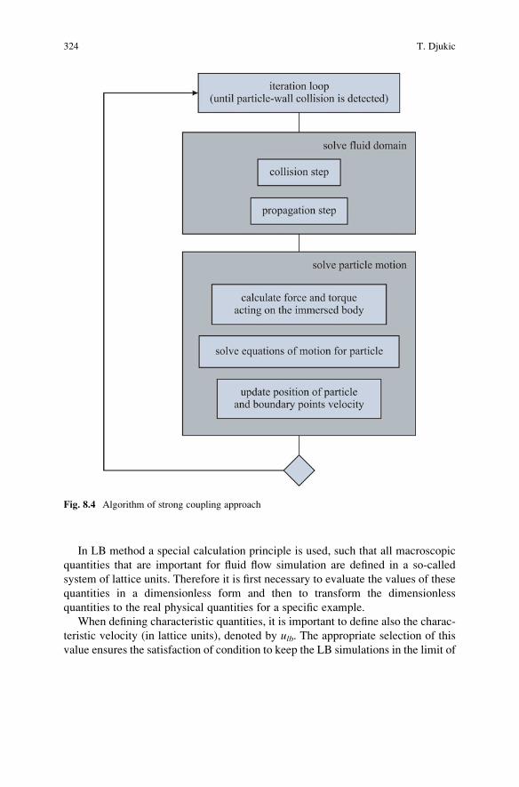
domain. Figure 8.4 shows a schematic diagram of the strong coupling approach

in modeling nanoparticles motion using immersed boundary method.

8.4 Numerical Results

Specialized and in-house developed software that numerically simulates fluid flow

using the principles of LB method is used to simulate several problems of particle

movement through fluid domain. Obtained results were compared with the analyti-

cal solutions or with results obtained using other methods that were found in

literature.

All examples are related to two-dimensional (plane) problems and that is why

the lattice denoted by D2Q9 was used for the simulations. For every example

several characteristic quantities need to be defined. First, it is necessary to define

resolution N that represents the number of nodes along one direction (most com-

monly it is the y axis direction). The domain is defined using characteristic lengths

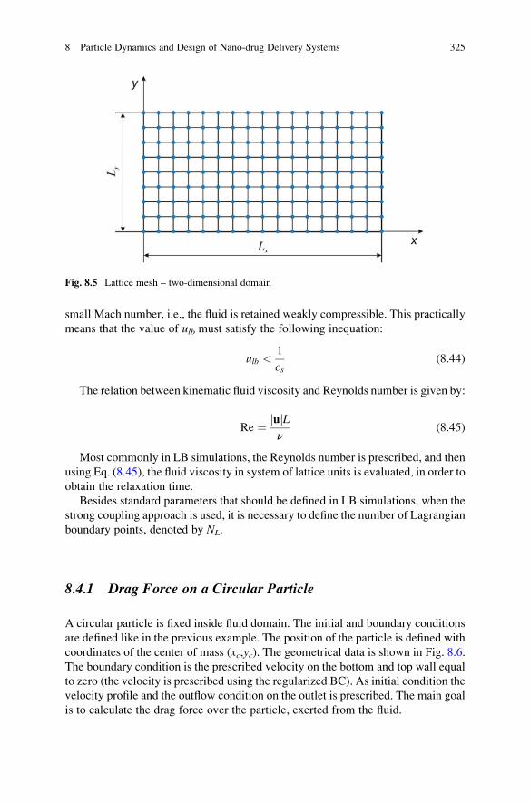
lx and ly, while “physical” lengths, denoted by Lx and Ly, are calculated as:

Lx ¼ lx � N (8.42)

Ly ¼ ly � N (8.43)

Figure 8.5 shows one domain, and the coordinate axes and mentioned lengths are

labeled.


In LB method a special calculation principle is used, such that all macroscopic

quantities that are important for fluid flow simulation are defined in a so-called

system of lattice units. Therefore it is first necessary to evaluate the values of these

quantities in a dimensionless form and then to transform the dimensionless

quantities to the real physical quantities for a specific example.

When defining characteristic quantities, it is important to define also the charac-

teristic velocity (in lattice units), denoted by ulb. The appropriate selection of this

value ensures the satisfaction of condition to keep the LB simulations in the limit of

Fig. 8.4 Algorithm of strong coupling approach

324 T. Djukic

small Mach number, i.e., the fluid is retained weakly compressible. This practically

means that the value of ulb must satisfy the following inequation:

ulb <1

cs(8.44)

The relation between kinematic fluid viscosity and Reynolds number is given by:

Re ¼ uj jLν

(8.45)

Most commonly in LB simulations, the Reynolds number is prescribed, and then

using Eq. (8.45), the fluid viscosity in system of lattice units is evaluated, in order to

obtain the relaxation time.

Besides standard parameters that should be defined in LB simulations, when the

strong coupling approach is used, it is necessary to define the number of Lagrangian

boundary points, denoted by NL.

8.4.1 Drag Force on a Circular Particle

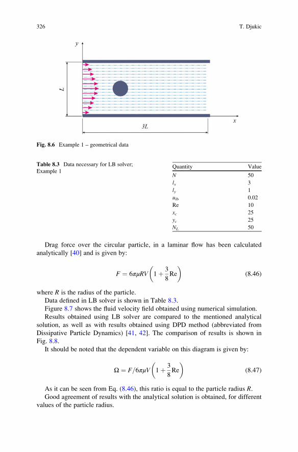
A circular particle is fixed inside fluid domain. The initial and boundary conditions

are defined like in the previous example. The position of the particle is defined with

coordinates of the center of mass (xc,yc). The geometrical data is shown in Fig. 8.6.

The boundary condition is the prescribed velocity on the bottom and top wall equal

to zero (the velocity is prescribed using the regularized BC). As initial condition the

velocity profile and the outflow condition on the outlet is prescribed. The main goal

is to calculate the drag force over the particle, exerted from the fluid.

Fig. 8.5 Lattice mesh – two-dimensional domain


Drag force over the circular particle, in a laminar flow has been calculated

analytically [40] and is given by:

F ¼ 6πμRV 1þ 3

8Re

� �(8.46)

where R is the radius of the particle.

Data defined in LB solver is shown in Table 8.3.

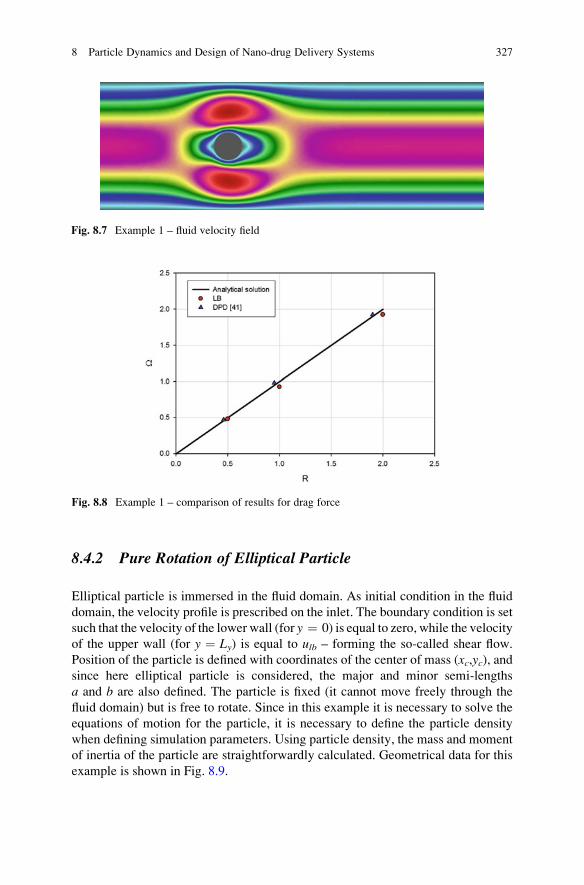
Figure 8.7 shows the fluid velocity field obtained using numerical simulation.

Results obtained using LB solver are compared to the mentioned analytical

solution, as well as with results obtained using DPD method (abbreviated from

Dissipative Particle Dynamics) [41, 42]. The comparison of results is shown in

Fig. 8.8.

It should be noted that the dependent variable on this diagram is given by:

Ω ¼ F=6πμV 1þ 3

8Re

� �(8.47)

As it can be seen from Eq. (8.46), this ratio is equal to the particle radius R.Good agreement of results with the analytical solution is obtained, for different

values of the particle radius.

Fig. 8.6 Example 1 – geometrical data

Table 8.3 Data necessary for LB solver;

Example 1Quantity Value

N 50

lx 3

ly 1

ulb 0.02

Re 10

xc 25

yc 25

NL 50

326 T. Djukic

8.4.2 Pure Rotation of Elliptical Particle

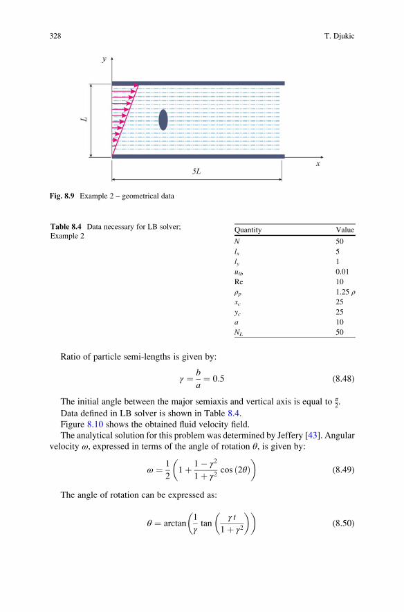
Elliptical particle is immersed in the fluid domain. As initial condition in the fluid

domain, the velocity profile is prescribed on the inlet. The boundary condition is set

such that the velocity of the lower wall (for y ¼ 0) is equal to zero, while the velocity

of the upper wall (for y ¼ Ly) is equal to ulb – forming the so-called shear flow.

Position of the particle is defined with coordinates of the center of mass (xc,yc), andsince here elliptical particle is considered, the major and minor semi-lengths

a and b are also defined. The particle is fixed (it cannot move freely through the

fluid domain) but is free to rotate. Since in this example it is necessary to solve the

equations of motion for the particle, it is necessary to define the particle density

when defining simulation parameters. Using particle density, the mass and moment

of inertia of the particle are straightforwardly calculated. Geometrical data for this

example is shown in Fig. 8.9.

Fig. 8.7 Example 1 – fluid velocity field

Fig. 8.8 Example 1 – comparison of results for drag force


Ratio of particle semi-lengths is given by:

γ ¼ b

a¼ 0:5 (8.48)

The initial angle between the major semiaxis and vertical axis is equal to π2.


Figure 8.10 shows the obtained fluid velocity field.

The analytical solution for this problem was determined by Jeffery [43]. Angular

velocity ω, expressed in terms of the angle of rotation θ, is given by:

ω ¼ 1

21þ 1� γ2

1þ γ2cos 2θð Þ

� �(8.49)

The angle of rotation can be expressed as:

θ ¼ arctan1

γtan

γ t

1þ γ2

� �� (8.50)




N 50

lx 5

ly 1

ulb 0.01

Re 10

ρp 1.25 ρxc 25

yc 25

a 10

NL 50

328 T. Djukic

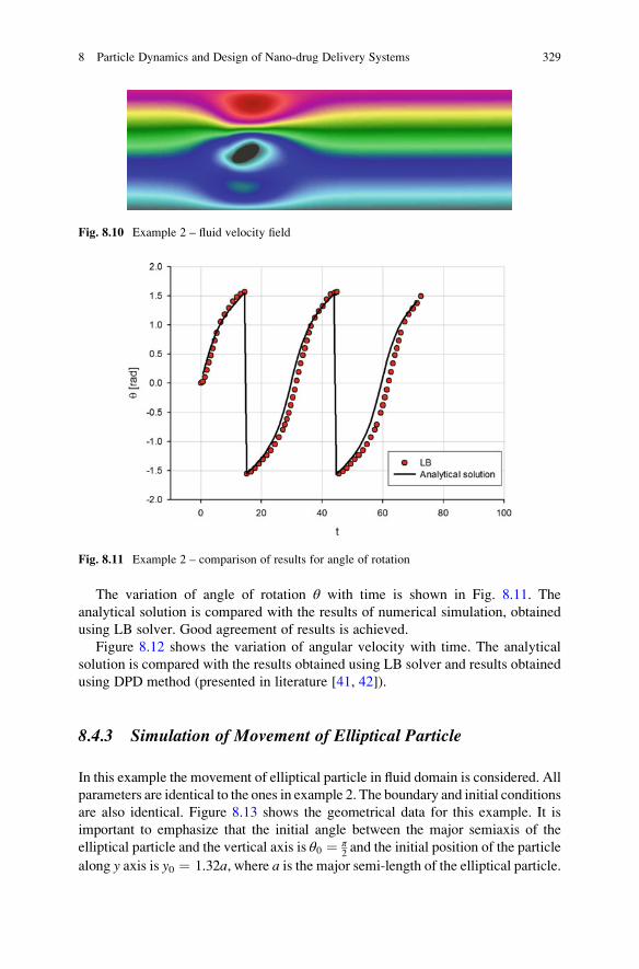
The variation of angle of rotation θ with time is shown in Fig. 8.11. The

analytical solution is compared with the results of numerical simulation, obtained

using LB solver. Good agreement of results is achieved.

Figure 8.12 shows the variation of angular velocity with time. The analytical

solution is compared with the results obtained using LB solver and results obtained

using DPD method (presented in literature [41, 42]).

8.4.3 Simulation of Movement of Elliptical Particle

In this example the movement of elliptical particle in fluid domain is considered. All

parameters are identical to the ones in example 2. The boundary and initial conditions

are also identical. Figure 8.13 shows the geometrical data for this example. It is

important to emphasize that the initial angle between the major semiaxis of the

elliptical particle and the vertical axis is θ0 ¼ π2and the initial position of the particle

along y axis is y0 ¼ 1.32a, where a is the major semi-length of the elliptical particle.


Fig. 8.11 Example 2 – comparison of results for angle of rotation


The Stokes number has a great influence on the particle trajectory. Stokes

number is defined by:

St ¼ ρpb2S

μ(8.51)

where ρp is the particle density.The relation between Stokes and Reynolds number is given by:

St ¼ ρpρRe (8.52)

Fig. 8.12 Example 2 – comparison of results for angular velocity


330 T. Djukic

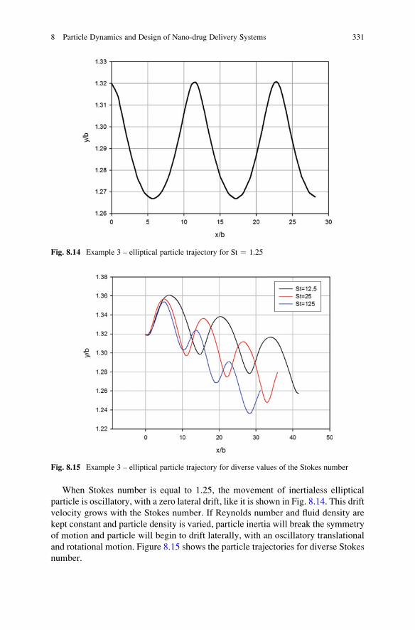
When Stokes number is equal to 1.25, the movement of inertialess elliptical

particle is oscillatory, with a zero lateral drift, like it is shown in Fig. 8.14. This drift

velocity grows with the Stokes number. If Reynolds number and fluid density are

kept constant and particle density is varied, particle inertia will break the symmetry

of motion and particle will begin to drift laterally, with an oscillatory translational

and rotational motion. Figure 8.15 shows the particle trajectories for diverse Stokes

number.

Fig. 8.14 Example 3 – elliptical particle trajectory for St ¼ 1.25

Fig. 8.15 Example 3 – elliptical particle trajectory for diverse values of the Stokes number


In the design of nano-drug delivery systems, these observations should be

considered. Both spherical and nonspherical particles with appropriate mass and

geometrical inertia will drift on their way through blood vessels and hence will be

able to sense abnormalities in vessel walls.

8.4.4 Simulation of Movement of a Circular Particle inLinear Shear Flow

A circular particle is immersed in fluid domain and is free to move. As boundary

condition the velocity of upper and lower wall is prescribed to be equal to ulb, and thewalls are moving in opposite directions. As initial condition the velocity profile on the

inlet is defined, the so-called double shear flow. The geometrical data is shown in

Fig. 8.16. In this example it is considered that solid and fluid densities are equal. The

initial position of the particle is defined with coordinates of the center of mass (xc,yc),and the particle radius r is also defined. It should be noted that the initial position

of the particle is defined such that the particle is located at L4above the bottom wall.





N 80

lx 10

ly 1

ulb 0.0375

Re 40

xc 50

yc 20

r 10

NL 50

332 T. Djukic

This problem was first investigated by Feng et al. [44] (and simulated using finite

element method), and they concluded that no matter how the particle is initially

positioned, it always tends to migrate to the centerline of the channel. Later this

same problem has been studied by others and simulated using other methods,

including LB method and diverse approaches for solid–fluid interaction. Here the

obtained results were compared to the results presented in literature [33, 35, 38].

Figure 8.17 shows the fluid velocity field during particle movement.

Figures 8.18, 8.19, and 8.20 show comparison of results obtained using the

developed LB solver with results found in literature, for movement of particle in

y axis direction and the components of translational velocities in x and y axis

direction. On all three diagrams, the dimensionless values obtained in simulations

are shown on both axes.


Fig. 8.18 Example 4 – comparison of results for particle position in y axis direction


8.4.5 Particle Sedimentation in Viscous Fluid

This example illustrates the movement of particle due to gravity force. At the

beginning of the simulation, the circular particle and fluid are in static state (the

initial velocity of the particle as well as fluid velocity in all lattice nodes are equal to

zero). Particle is located at the middle of fluid domain along horizontal axis and at 23

Fig. 8.19 Example 4 – comparison of results for x component of particle velocity

Fig. 8.20 Example 4 – comparison of results for y component of particle velocity

334 T. Djukic

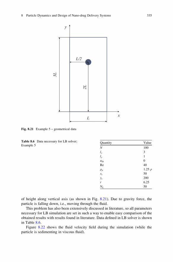
of height along vertical axis (as shown in Fig. 8.21). Due to gravity force, the

particle is falling down, i.e., moving through the fluid.

This problem has also been extensively discussed in literature, so all parameters

necessary for LB simulation are set in such a way to enable easy comparison of the

obtained results with results found in literature. Data defined in LB solver is shown

in Table 8.6.

Figure 8.22 shows the fluid velocity field during the simulation (while the

particle is sedimenting in viscous fluid).




N 100

lx 3

ly 1

ulb 0

Re 40

ρp 1.25 ρxc 50

yc 200

r 6.25

NL 50


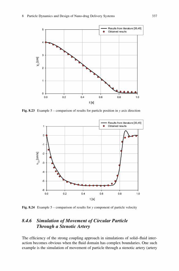
Results obtained using LB solver are compared with results presented by

Wu et al. [35] (the simulation was performed using LB method), as well as with

results presented by Wan and Turek [45] (the simulation was performed using finite

element method). The variations of four quantities are observed – the position of

particle in y axis direction, y component of particle velocity, Reynolds number, and

translational kinetic energy. Reynolds number in a specified moment in time can be

evaluated using the following expression:

Re ¼ρpr

ffiffiffiffiffiffiffiffiffiffiffiffiffiffiffiffiffiffiffiv2Cx þ v2Cy

qμ

(8.53)

The expression for the translational kinetic energy in a specific moment in time

is given by:

Et ¼ 1

2m v2Cx þ v2Cy

� �(8.54)

As it can be seen from Figs. 8.23, 8.24, 8.25, and 8.26, the obtained results

compare very well with results found in literature.

Fig. 8.22 Example 5 –

fluid velocity field

336 T. Djukic

8.4.6 Simulation of Movement of Circular ParticleThrough a Stenotic Artery

The efficiency of the strong coupling approach in simulations of solid–fluid inter-

action becomes obvious when the fluid domain has complex boundaries. One such

example is the simulation of movement of particle through a stenotic artery (artery

Fig. 8.23 Example 5 – comparison of results for particle position in y axis direction



with constriction). Li et al. [46] have analyzed the pulsatile flow in a mildly or

severely stenotic artery, and Wu and Shu simulated the motion of particles through

stenotic artery in one of their papers [35]. Therefore here the results found in

literature will be compared with results obtained using LB solver.

Fig. 8.25 Example 5 – comparison of results for Reynolds number

Fig. 8.26 Example 5 – comparison of results for translational kinetic energy

338 T. Djukic

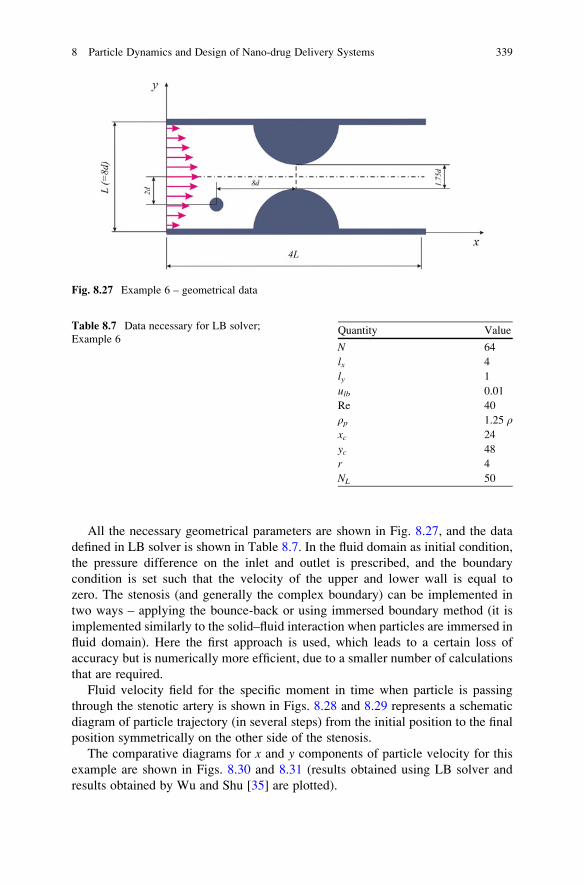
All the necessary geometrical parameters are shown in Fig. 8.27, and the data

defined in LB solver is shown in Table 8.7. In the fluid domain as initial condition,

the pressure difference on the inlet and outlet is prescribed, and the boundary

condition is set such that the velocity of the upper and lower wall is equal to

zero. The stenosis (and generally the complex boundary) can be implemented in

two ways – applying the bounce-back or using immersed boundary method (it is

implemented similarly to the solid–fluid interaction when particles are immersed in

fluid domain). Here the first approach is used, which leads to a certain loss of

accuracy but is numerically more efficient, due to a smaller number of calculations

that are required.

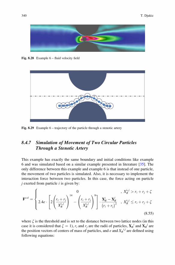
Fluid velocity field for the specific moment in time when particle is passing

through the stenotic artery is shown in Figs. 8.28 and 8.29 represents a schematic

diagram of particle trajectory (in several steps) from the initial position to the final

position symmetrically on the other side of the stenosis.

The comparative diagrams for x and y components of particle velocity for this

example are shown in Figs. 8.30 and 8.31 (results obtained using LB solver and

results obtained by Wu and Shu [35] are plotted).




N 64

lx 4

ly 1

ulb 0.01

Re 40

ρp 1.25 ρxc 24

yc 48

r 4

NL 50


8.4.7 Simulation of Movement of Two Circular ParticlesThrough a Stenotic Artery

This example has exactly the same boundary and initial conditions like example

6 and was simulated based on a similar example presented in literature [35]. The

only difference between this example and example 6 is that instead of one particle,

the movement of two particles is simulated. Also, it is necessary to implement the

interaction force between two particles. In this case, the force acting on particle

j exerted from particle i is given by:

Fcol ¼0 , Xi, j

R > ri þ rj þ ζ

2:4ε � 2ri þ rj

Xi, jR

0@

1A

14

� ri þ rj

Xi, jR

0@

1A

824

35 � X

iR � X

jR

ri þ rj� �2 , Xi, j

R � ri þ rj þ ζ

8>>><>>>:

(8.55)

where ζ is the threshold and is set to the distance between two lattice nodes (in thiscase it is considered that ζ ¼ 1), ri and rj are the radii of particles, XR

i and XRj are

the position vectors of centers of mass of particles, аnd ε and XRi,j are defined using

following equations:


Fig. 8.29 Example 6 – trajectory of the particle through a stenotic artery

340 T. Djukic

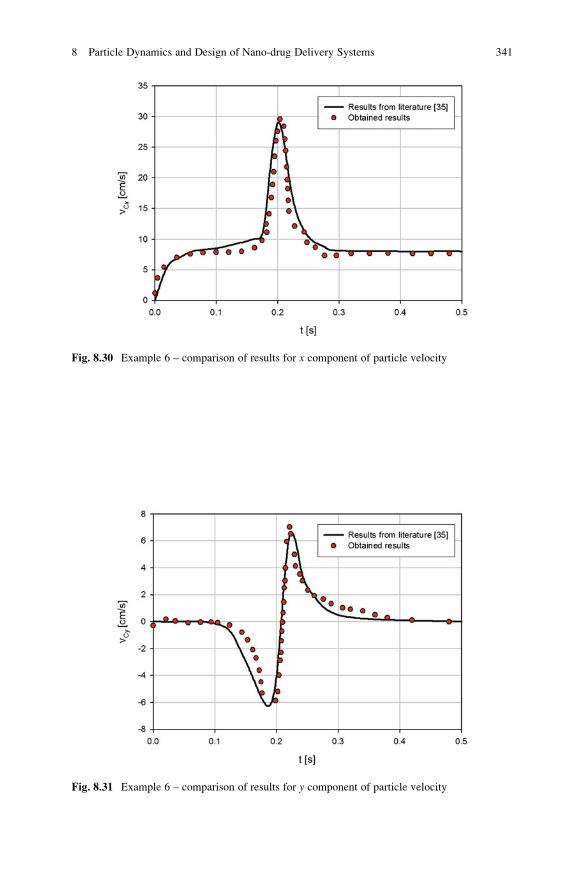
Fig. 8.30 Example 6 – comparison of results for x component of particle velocity



ε ¼ 2rirjri þ rj

� �2

(8.56)

Xi, jR ¼ Xi

R � XjR

�� (8.57)

When the interaction force is calculated, it is added in the expression for total

force acting on every particle individually (Eq. (8.39)) and then the equations of

motion are solved. The total force is now given by:

FR ¼ 1� ρfρp

!mGþ Fcol �

Xl

F XlB

� �Δsl (8.58)

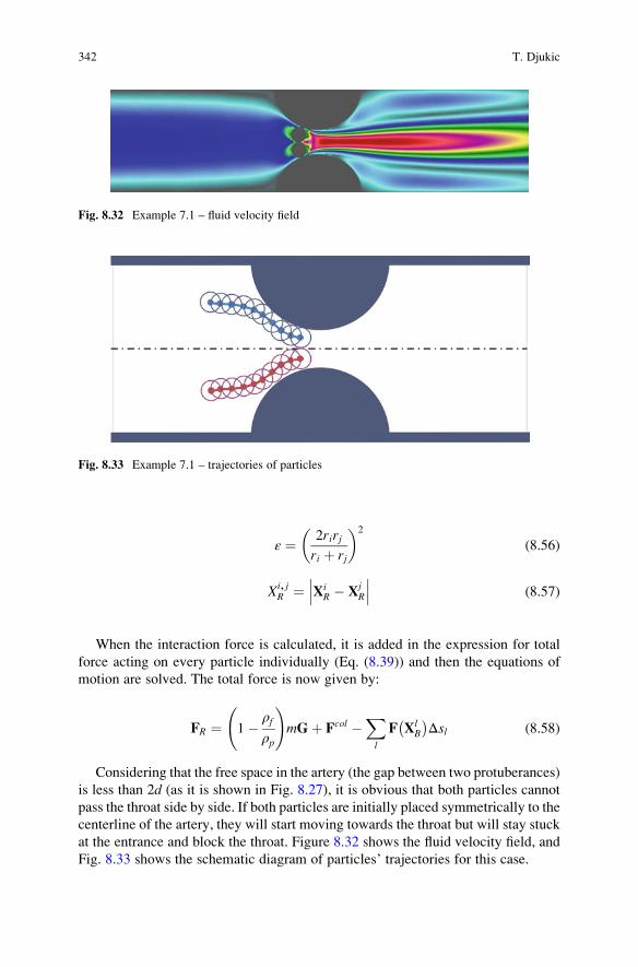
Considering that the free space in the artery (the gap between two protuberances)

is less than 2d (as it is shown in Fig. 8.27), it is obvious that both particles cannot

pass the throat side by side. If both particles are initially placed symmetrically to the

centerline of the artery, they will start moving towards the throat but will stay stuck

at the entrance and block the throat. Figure 8.32 shows the fluid velocity field, and

Fig. 8.33 shows the schematic diagram of particles’ trajectories for this case.

Fig. 8.32 Example 7.1 – fluid velocity field

Fig. 8.33 Example 7.1 – trajectories of particles

342 T. Djukic

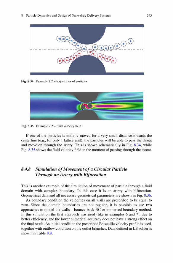
If one of the particles is initially moved for a very small distance towards the

centerline (e.g., for only 1 lattice unit), the particles will be able to pass the throat

and move on through the artery. This is shown schematically in Fig. 8.34, while

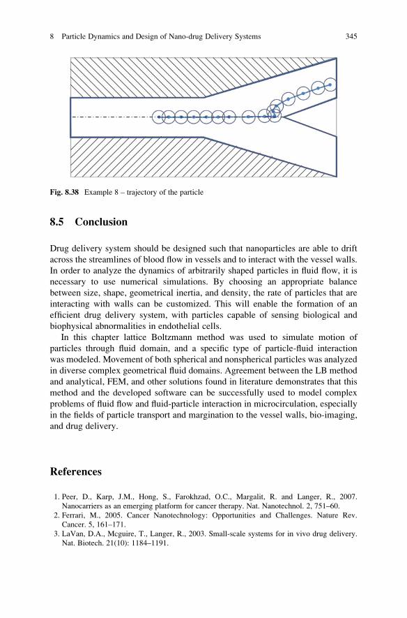
Fig. 8.35 shows the fluid velocity field in the moment of passing through the throat.

8.4.8 Simulation of Movement of a Circular ParticleThrough an Artery with Bifurcation

This is another example of the simulation of movement of particle through a fluid

domain with complex boundary. In this case it is an artery with bifurcation.

Geometrical data and all necessary geometrical parameters are shown in Fig. 8.36.

As boundary condition the velocities on all walls are prescribed to be equal to

zero. Since the domain boundaries are not regular, it is possible to use two

approaches to model the walls – bounce-back BC or immersed boundary method.

In this simulation the first approach was used (like in examples 6 and 7), due to

better efficiency, and the lower numerical accuracy does not have a strong effect on

the final result. As initial condition the prescribed Poiseuille velocity profile is used,

together with outflow condition on the outlet branches. Data defined in LB solver is

shown in Table 8.8.

Fig. 8.34 Example 7.2 – trajectories of particles

Fig. 8.35 Example 7.2 – fluid velocity field


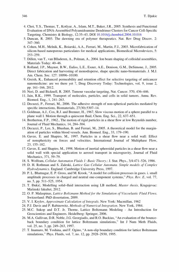
When the particle starts moving, it comes across the bifurcation. Strong repul-

sive force is acting on the particle so that it rebounds from the wall and continues to

move through the upper branch, until the end of the domain. Figure 8.37 shows the

fluid velocity field during the motion of particle through the main branch of the

artery, and Fig. 8.38 shows schematically the trajectory of the particle.



N 60

lx 3

ly 1

ulb 0.01

Re 40

ρp 1.25 ρxc 60

yc 30

r 3

NL 20



344 T. Djukic

8.5 Conclusion

Drug delivery system should be designed such that nanoparticles are able to drift

across the streamlines of blood flow in vessels and to interact with the vessel walls.

In order to analyze the dynamics of arbitrarily shaped particles in fluid flow, it is

necessary to use numerical simulations. By choosing an appropriate balance

between size, shape, geometrical inertia, and density, the rate of particles that are

interacting with walls can be customized. This will enable the formation of an

efficient drug delivery system, with particles capable of sensing biological and

biophysical abnormalities in endothelial cells.

In this chapter lattice Boltzmann method was used to simulate motion of

particles through fluid domain, and a specific type of particle-fluid interaction

was modeled. Movement of both spherical and nonspherical particles was analyzed

in diverse complex geometrical fluid domains. Agreement between the LB method

and analytical, FEM, and other solutions found in literature demonstrates that this

method and the developed software can be successfully used to model complex

problems of fluid flow and fluid-particle interaction in microcirculation, especially

in the fields of particle transport and margination to the vessel walls, bio-imaging,

and drug delivery.

References

1. Peer, D., Karp, J.M., Hong, S., Farokhzad, O.C., Margalit, R. and Langer, R., 2007.

Nanocarriers as an emerging platform for cancer therapy. Nat. Nanotechnol. 2, 751–60.

2. Ferrari, M., 2005. Cancer Nanotechnology: Opportunities and Challenges. Nature Rev.

Cancer. 5, 161–171.

3. LaVan, D.A., Mcguire, T., Langer, R., 2003. Small-scale systems for in vivo drug delivery.

Nat. Biotech. 21(10): 1184–1191.

Fig. 8.38 Example 8 – trajectory of the particle


4. Choi, Y.S., Thomas, T., Kotlyar, A., Islam, M.T., Baker, J.R., 2005. Synthesis and Functional

Evaluation of DNA-Assembled Polyamidoamine Dendrimer Clusters for Cancer Cell-Specific

Targeting. Chemistry & Biology, 12:35–43, DOI 10.1016/j.chembiol.2004.10.016

5. Duncan, R. 2003. The dawning era of polymer therapeutics. Nat. Rev Drug Discov. 2:

347–360.

6. Cohen, M.H., Melnik, K., Boiarski, A.A., Ferrari, M., Martin, F.J., 2003. Microfabrication of

silicon-based nanoporous particulates for medical applications, Biomedical Microdevices, 5:

253–259.

7. Dillen, van T., van Blladeren, A., Polman, A., 2004. Ion beam shaping of colloidal assemblies,

Materials Today: 40–46.

8. Rolland, J.P., Maynor, B.W., Euliss, L.E., Exner, A.E., Denison, G.M., DeSimone, J., 2005.

Direct fabrication and harvesting of monodisperse, shape specific nano-biomaterials. J. M.J.

Am. Chem. Soc. 127: 10096–10100.

9. Greish, K., Enhanced permeability and retention effect for selective targeting of anticancer

nanomedicine: are we there yet ?, Drug Discovery Today: Technologies, vol. 9, issue 2,

pp. 161–166, 2012.

10. Neri, D. and Bicknell, R. 2005. Tumour vascular targeting, Nat. Cancer. 570, 436–446.

11. Jain, R.K., 1999. Transport of molecules, particles, and cells in solid tumors. Annu. Rev.

Biomed. Eng., 1, 241–263.

12. Decuzzi, P., Ferrari, M., 2006. The adhesive strength of non-spherical particles mediated by

specific interactions, Biomaterials, 27(30):5307–14.

13. Goldman, A.J., Cox, R.J. and Brenner, H., 1967, Slow viscous motion of a sphere parallel to a

plane wall I. Motion through a quiescent fluid, Chem. Eng. Sci., 22, 637–651.

14. Bretherton, F.P., 1962., The motion of rigid particles in a shear flow at low Reynolds number,

Journal of Fluid Mechanics, 14, 284–304.

15. Decuzzi, P., Lee, S., Bhushan, B. and Ferrari, M., 2005. A theoretical model for the margin-

ation of particles within blood vessels. Ann. Biomed. Eng., 33, 179–190.

16. Gavze, E. and Shapiro, M., 1997. Particles in a shear flow near a solid wall: Effect

of nonsphericity on forces and velocities. International Journal of Multiphase Flow,

23, 155–182.

17. Gavze, E. and Shapiro, M., 1998. Motion of inertial spheroidal particles in a shear flow near a

solid wall with special application to aerosol transport in microgravity, Journal of Fluid

Mechanics, 371, 59–79.

18. S. Wolfram, Cellular Automaton Fluids 1: Basic Theory.: J. Stat. Phys., 3/4:471–526, 1986.19. D. H. Rothman and S. Zaleski, Lattice Gas Cellular Automata. Simple models of Complex

Hydrodynamics. England: Cambridge University Press, 1997.

20. P. L. Bhatnagar, E. P. Gross, and M. Krook, “A model for collision processes in gases. i. small

amplitude processes in charged and neutral one-component systems,” Phys. Rev. E, vol. 77,no. 5, pp. 511–525, 1954.

21. T. Ðukic, Modelling solid–fluid interaction using LB method, Master thesis, Kragujevac:Masinski fakultet, 2012.

22. O. P. Malaspinas, Lattice Boltzmann Method for the Simulation of Viscoelastic Fluid Flows.Switzerland: PhD dissertation, 2009.

23. V. I. Krylov, Approximate Calculation of Integrals. New York: Macmillan, 1962

24. P.J. Davis and P. Rabinowitz, Mеthods of Numerical Integration. New York, 1984.

25. M.C. Sukop and D.T. Jr. Thorne, Lattice Boltzmann Modeling - An Introduction for

Geoscientists and Engineers. Heidelberg: Springer, 2006.

26. M.A. Gallivan, D.R. Noble, J.G. Georgiadis, and R.O. Buckius, “An evaluation of the bounce-

back boundary condition for lattice Boltzmann simulations,” Int J Num Meth Fluids,

vol. 25, no. 3, pp. 249–263, 1997.

27. T. Inamuro, M. Yoshina, and F. Ogino, “A non-slip boundary condition for lattice Boltzmann

simulations,” Phys. Fluids, vol. 7, no. 12, pp. 2928–2930, 1995.

346 T. Djukic

http://dx.doi.org/10.1016/j.chembiol.2004.10.016

28. I. Ginzbourg and D. d ‘Humieres, “Local second-order boundary method for lattice Boltzmann

models,” J. Statist. Phys., vol. 84, no. 5–6, pp. 927–971, 1996.

29. B. Chopard and A. Dupuis, “A mass conserving boundary condition for lattice Boltzmann

models,” Int. J. Mod. Phys. B, vol. 17, no. 1/2, pp. 103–108, 2003.

30. Q. Zou and X. He, “On pressure and velocity boundary conditions for the lattice Boltzmann

BGK model,” Phys. Fluids, vol. 9, no. 6, pp. 1592–1598, 1997.

31. J. Latt and B. Chopard, “Lattice Boltzmann method with regularized non-equilibrium distri-

bution functions,” Math. Comp. Sim., vol. 72, no. 1, pp. 165–168, 2006.

32. P.A. Skordos, “Initial and boundary conditions for the lattice Boltzmann method,” Phys.

Rev. E, vol. 48, no. 6, pp. 4823–4842, 1993.

33. Z. Feng and E. Michaelides, “The immersed boundary-lattice Boltzmann method for solving

fluid-particles interaction problem,” Journal of Computational Physics, vol. 195, no. 2,

pp. 602–628, 2004.

34. C. S. Peskin, “Numerical analysis of blood flow in the heart,” Journal of Computational

Physics, vol. 25, no. 3, pp. 220–252, 1977.

35. J. Wu and C. Shu, “Particulate flow simulation via a boundary condition-enforced immersed

boundary-lattice Boltzmann scheme,” Commun. Comput. Phys., vol. 7, no. 4, pp. 793–812,

2010.

36. Z. Feng and E. Michaelides, “Proteus: A direct forcing method in the simulations of particulate

flows,” Journal of Computational Physics, vol. 202, no. 1, pp. 20–51, 2005.

37. M. Uhlmann, “An immersed boundary method with direct forcing for the simulation of

particulate flows,” J. Comput. Phys., vol. 209, no. 2, pp. 448–476, 2005.

38. X. D. Niu, C. Shu, Y. T. Chew, and Y. Peng, “A momentum exchange-based immersed

boundary-lattice Boltzmann method for simulating incompressible viscous flows,” Phys.

Lett. A, vol. 354, no. 3, pp. 173–182, 2006.

39. J. Wu and C. Shu, “Implicit velocity correction-based immersed boundary-lattice Boltzmann

method and its application,” J. Comput. Phys., vol. 228, no. 6, pp. 1963–1979, 2009.

40. A. T. Chwang and T. Y. Wu, “Hydromechanics of low-Reynolds-number flow, Part 4, Trans-

lation of spheroids,” J. Fluid Mech., vol. 75, no. 4, pp. 677–689, 1976.

41. N. Filipovic, M. Kojic, P. Decuzzi, and M. Ferrari, “Dissipative Particle Dynamics simulation

of circular and elliptical particles motion in 2D laminar shear flow,” Microfluidics and

Nanofluidics, vol. 10, no. 5, pp. 1127–1134, 2010.

42. N. Filipovic, V. Isailovic, T. Djukic, M. Ferrari, and M. Kojic, “Multi-scale modeling of

circular and elliptical particles in laminar shear flow,” IEEE Trans Biomed Eng, vol. 59,

no. 1, pp. 50–53, 2012.

43. G. B. Jeffery, “The motion of ellipsoidal particles immersed in a viscous fluid,” Proc. R. Soc.

Lond. A, vol. 102, no. 715, pp. 161–180, 1922.

44. J. Feng, H. H. Hu, and D. D. Joseph, “Direct simulation of initial value problems for the motion

of solid bodies in a Newtonian fluid. Part 2, Couette and Poiseuille flows,” J. Fluid Mech.,

vol. 277, pp. 271–301, 1994.

45. D. Wan and S. Turek, “Direct numerical simulation of particulate flow via multigrid FEM

techniques and the fictitious boundary method,” Int. J. Numer. Meth. Fluids, vol. 51, no. 5,pp. 531–566, 2006.

46. H. Li, H. Fang, Z. Lin, S. Xu, and S. Chen, “Lattice Boltzmann simulation on particle

suspensions in a two-dimensional symmetric stenotic artery,” Phys. Rev. E, vol. 69,

no. 3, p. 031919, 2004.


computational medicine in data mining and modeling || particle dynamics and design of nano-drug...

Documents