computational methods applied to superconductivity and...
TRANSCRIPT

Computational methods applied to Superconductivity and Magnetism
By
Alan KykerB.S. (University of Tennessee at Knoxville) 1988
DISSERTATION
Submitted in partial satisfaction of the requirements for the degree of
Doctor of Philosophy
in
Physics
in the
OFFICE OF GRADUATE STUDIES
of the
UNIVERSITY OF CALIFORNIADAVIS
Approved:
Committee in Charge
2006
i

To Dale
ii

Abstract
Computational methods applied to Superconductivity and Magnetism
by
Alan Kyker
Superconductivity and magnetism are two phenomena where the microscope quantum
world manifests macroscopic visible behavior. The methods of studying these condensates
generally follow a quantum mechanical (bottom up) or phenomenological (top down). In
principal, bottom up methods are sufficient to describe all behavior, but in practice the cal-
culations become intractable. The effect of electronic structure on the formation of FFLO
phases was studied using a modified BCS formalism. Features of the Fermi surfaces which
promoted the formation of FFLO phases were identified. Magnetically induced orbital
currents, vortex dynamics and multi-order parameter superconductors were studied using
the phenomenological formalism of Ginzburg and Landau. A new topological structure
was identified in multi-order parameter superconductors with Josephson coupling. The
electronic structure tools the were developed for studying FFLO phases were then applied
TiBe2. The source of the anomalous temperature dependent susceptibility was identified.
Classical magnetism was studied using transfer matrix methods. A method was devel-
oped for extracting the density of states for long, narrow, nearest neighbor, 2D Ising and
Edwards-Anderson spin systems.
iii

iv

Contents
List of Figures vii
1 Theory of ~q 6= 0 Pairing Superconductivity 1
1.1 Introduction . . . . . . . . . . . . . . . . . . . . . . . . . . . . . . . . . . . . 21.2 Cooper Pair . . . . . . . . . . . . . . . . . . . . . . . . . . . . . . . . . . . . 61.3 BCS . . . . . . . . . . . . . . . . . . . . . . . . . . . . . . . . . . . . . . . . 91.4 Bogoliubov-Valatin transformation . . . . . . . . . . . . . . . . . . . . . . . 111.5 The Gap equation . . . . . . . . . . . . . . . . . . . . . . . . . . . . . . . . 151.6 BCS Phase . . . . . . . . . . . . . . . . . . . . . . . . . . . . . . . . . . . . 161.7 FFLO Phase . . . . . . . . . . . . . . . . . . . . . . . . . . . . . . . . . . . 181.8 Applications of Nesting Density to FFLO calculations . . . . . . . . . . . . 231.9 1D Fermi Surface . . . . . . . . . . . . . . . . . . . . . . . . . . . . . . . . . 241.10 2D Fermi Surface . . . . . . . . . . . . . . . . . . . . . . . . . . . . . . . . . 251.11 3D Fermi Surface . . . . . . . . . . . . . . . . . . . . . . . . . . . . . . . . . 271.12 ZrZn2 . . . . . . . . . . . . . . . . . . . . . . . . . . . . . . . . . . . . . . . 301.13 Conclusion . . . . . . . . . . . . . . . . . . . . . . . . . . . . . . . . . . . . 341.14 Free energy calculations . . . . . . . . . . . . . . . . . . . . . . . . . . . . . 351.15 Numerical methods . . . . . . . . . . . . . . . . . . . . . . . . . . . . . . . . 36
2 Fermi Velocity and Incipient Magnetism in TiBe2 39
2.1 Introduction . . . . . . . . . . . . . . . . . . . . . . . . . . . . . . . . . . . . 402.2 Crystal Structure . . . . . . . . . . . . . . . . . . . . . . . . . . . . . . . . . 432.3 Method of Calculations . . . . . . . . . . . . . . . . . . . . . . . . . . . . . 442.4 Results and Discussions . . . . . . . . . . . . . . . . . . . . . . . . . . . . . 452.5 Analysis of Velocity Distribution and Susceptibility . . . . . . . . . . . . . . 532.6 Summary . . . . . . . . . . . . . . . . . . . . . . . . . . . . . . . . . . . . . 64
3 Macroscopic Theory of Multi Order Parameter Pairing in Superconduc-
tiity 67
3.1 Multi Order Parameter Landau Theory . . . . . . . . . . . . . . . . . . . . 68
v

3.2 Ginzburg-Landau Theory . . . . . . . . . . . . . . . . . . . . . . . . . . . . 723.3 Multi-Order Parameter Ginzburg-Landau Theory . . . . . . . . . . . . . . . 763.4 Solving the Ginzburg-Landau Model . . . . . . . . . . . . . . . . . . . . . . 783.5 Boundary Conditions and Simulation Controls. . . . . . . . . . . . . . . . . 803.6 The Vortex . . . . . . . . . . . . . . . . . . . . . . . . . . . . . . . . . . . . 823.7 Flux quantization of one order parameter . . . . . . . . . . . . . . . . . . . 853.8 Fractional flux quantization with two order parameters . . . . . . . . . . . . 883.9 The bi-quadratic term . . . . . . . . . . . . . . . . . . . . . . . . . . . . . . 913.10 The Josephson term . . . . . . . . . . . . . . . . . . . . . . . . . . . . . . . 933.11 J-wall excitations . . . . . . . . . . . . . . . . . . . . . . . . . . . . . . . . . 973.12 Not any knots . . . . . . . . . . . . . . . . . . . . . . . . . . . . . . . . . . . 983.13 Conclusion . . . . . . . . . . . . . . . . . . . . . . . . . . . . . . . . . . . . 100
4 Classical Spin Systems 101
4.1 Introduction . . . . . . . . . . . . . . . . . . . . . . . . . . . . . . . . . . . . 1024.2 Transfer matrix applied to spin systems. . . . . . . . . . . . . . . . . . . . . 1034.3 One spin at a time . . . . . . . . . . . . . . . . . . . . . . . . . . . . . . . . 1064.4 Finite T computations . . . . . . . . . . . . . . . . . . . . . . . . . . . . . . 1104.5 Partition function polynomial and T = 0 calculations . . . . . . . . . . . . . 1114.6 2D Ising phase transition . . . . . . . . . . . . . . . . . . . . . . . . . . . . 1134.7 Spin Glass . . . . . . . . . . . . . . . . . . . . . . . . . . . . . . . . . . . . . 1174.8 Trapping local energy minimum . . . . . . . . . . . . . . . . . . . . . . . . . 1174.9 Frustration . . . . . . . . . . . . . . . . . . . . . . . . . . . . . . . . . . . . 1184.10 2D ±1 glass simulations . . . . . . . . . . . . . . . . . . . . . . . . . . . . . 1214.11 2D continuous bond distribution glass simulation . . . . . . . . . . . . . . . 1244.12 Conclusion . . . . . . . . . . . . . . . . . . . . . . . . . . . . . . . . . . . . 128
Bibliography 129
vi

List of Figures
1.1 Quasiparticle density of states at Fermi level . . . . . . . . . . . . . . . . . 141.2 BCS phase diagram with ~q = 0 . . . . . . . . . . . . . . . . . . . . . . . . . 171.3 Quasiparticle nesting . . . . . . . . . . . . . . . . . . . . . . . . . . . . . . . 191.4 Gap-less density of states . . . . . . . . . . . . . . . . . . . . . . . . . . . . 201.5 Integral kernel . . . . . . . . . . . . . . . . . . . . . . . . . . . . . . . . . . 221.6 1D FFLO phase diagram . . . . . . . . . . . . . . . . . . . . . . . . . . . . 241.7 2D nesting density . . . . . . . . . . . . . . . . . . . . . . . . . . . . . . . . 261.8 2D FFLO phase diagram . . . . . . . . . . . . . . . . . . . . . . . . . . . . 261.9 Tight binding Fermi surface . . . . . . . . . . . . . . . . . . . . . . . . . . . 281.10 3D tight binding FFLP phase diagram . . . . . . . . . . . . . . . . . . . . . 291.11 ZrZn2 nesting density . . . . . . . . . . . . . . . . . . . . . . . . . . . . . . 321.12 ZrZn2 dominate Fermi surface . . . . . . . . . . . . . . . . . . . . . . . . . . 33
2.1 Full TiBe2 non-magnetic band structure . . . . . . . . . . . . . . . . . . . . 462.2 Expanded TiBe2 non-magnetic band structure . . . . . . . . . . . . . . . . . 472.3 TiBe2 DOS . . . . . . . . . . . . . . . . . . . . . . . . . . . . . . . . . . . . 482.4 Fermi Surfaces . . . . . . . . . . . . . . . . . . . . . . . . . . . . . . . . . . 492.5 Fermi velocity spectrum . . . . . . . . . . . . . . . . . . . . . . . . . . . . . 532.6 Fermi velocity moments . . . . . . . . . . . . . . . . . . . . . . . . . . . . . 542.7 χ(~q) . . . . . . . . . . . . . . . . . . . . . . . . . . . . . . . . . . . . . . . . 572.8 Temperature dependant DOS near Fermi Energy and susceptability . . . . 612.9 B dependant DOS at the Fermi level . . . . . . . . . . . . . . . . . . . . . . 62
3.1 Vortex Smoke Rings . . . . . . . . . . . . . . . . . . . . . . . . . . . . . . . 813.2 Single vortex in 2D simulation . . . . . . . . . . . . . . . . . . . . . . . . . 843.3 Two non-equilibrium 3D vortices . . . . . . . . . . . . . . . . . . . . . . . . 873.4 Current and field of single vortex in single order parameter simulation . . . 883.5 Phase graph of condensate with and without vortex . . . . . . . . . . . . . 893.6 Current and field of single vortex in two order parameter simulation . . . . 903.7 2D simulation of condensate competition . . . . . . . . . . . . . . . . . . . . 92
vii

3.8 Phase frustration caused by vortex separation in two condensate supercon-ductor . . . . . . . . . . . . . . . . . . . . . . . . . . . . . . . . . . . . . . . 94
3.9 Wall of frustration caused by vortex separation in two condensate super-conductor . . . . . . . . . . . . . . . . . . . . . . . . . . . . . . . . . . . . . 96
3.10 Vortex knot components . . . . . . . . . . . . . . . . . . . . . . . . . . . . . 99
4.1 Long narrow spin system with transfer matrix cuts. . . . . . . . . . . . . . . 1044.2 Long narrow spin system with overlapping cuts. . . . . . . . . . . . . . . . . 1074.3 Log of density of states for 12 by 70 FM Ising model. . . . . . . . . . . . . . 1154.4 Specific heat for a range of FM Ising systems. . . . . . . . . . . . . . . . . . 1164.5 Frustrated plackets . . . . . . . . . . . . . . . . . . . . . . . . . . . . . . . . 1204.6 Log of density of states for 12 by 70 FM Ising model. . . . . . . . . . . . . . 1224.7 Specific heat for a range of FM Ising systems. . . . . . . . . . . . . . . . . . 1234.8 Odd eigenvalue projection of 18 spin wide Gaussian spin strip . . . . . . . . 127
viii

Chapter 1
Theory of ~q 6= 0 Pairing
Superconductivity
1

CHAPTER 1. THEORY OF ~Q 6= 0 PAIRING SUPERCONDUCTIVITY 2
1.1 Introduction
The work in this chapter is derived from the publication
“Fermiology and Fulde-Ferrell-Larkin-Ovchinnikov Phase Formation”; A. B. Kyker, W.
E. Pickett, and F. Gygi, Phys. Rev. B 71, 224517 (2005).
Almost half a century ago Ginzburg addressed the question of possible super-
conductivity in ferromagnetic material[1], and studied the problems posed by orbital su-
percurrents within a material with intrinsic magnetic flux. About a decade later, and
armed with BCS theory[2], Fulde and Ferrell (FF)[3] and separately Larkin and Ovchin-
nikov (LO)[4] addressed the separate question with how a BCS superconductor copes with
an intrinsic spin splitting, which breaks the degeneracy of spin up and spin down Fermi
surfaces. Both FF and LO concluded that (neglecting orbital current effects) that there
is a superconducting phase (the “FFLO phase”) above the usual upper critical field Hc2
where superconductivity persists based on ~q 6= 0 (non-zero momentum) pairs and the
order parameter becomes inhomogeneous.
Since that time there has been a considerable number of papers exploring the
competition between, and possible coexistence of, the superconducting and magnetic long
range order parameters.[5] Full treatment requires consideration of both orbital and spin
effects, and for the most part theories have tended to suppose that one is dominant in a
particular system and concentrate on that one. Thus investigations have focused either on
the orbital effects such as spontaneous vortex phases, or on the exposition of the FFLO
phase without complications from vortex behavior. Much has been accomplished with

CHAPTER 1. THEORY OF ~Q 6= 0 PAIRING SUPERCONDUCTIVITY 3
this approach, although little in a material specific way that would allow theories to be
carefully tested. With regard to the FFLO phase, the move has been in the opposite
direction: make the system fit the idealizations of the theorists.
Two dimensional layered organic crystals provide the primary playground. With
negligible carrier hopping between layers and the magnetic field can be oriented nearly in-
plane, the competition between spin- and orbital-pairbreaking first studied theoretically by
Bulaevskii[6] can be probed. If the field lies precisely within the layer, orbital pairbreaking
vanishes leaving only a small exchange splitting (±µBB) to inhibit superconductivity. This
setup has led to strong evidence that a distinct high field, low temperature phase in κ-
(BEDT-TTF)2Cu(NCS)2 is an excellent candidate for an FFLO phase.[7] The observed
new phase seems consistent with theoretical expectations,[8] and is suggested to arise due
to a favorable Fermi surface shape.[7]
A less prosaic candidate, still within the quasi-two-dimensional realm, is λ-
(BETS)2FeCl4, which contains the conducting layers of BETS molecules and layers of Fe3+
magnetic ions. At ambient pressure it undergoes a transition to an antiferromagnetic in-
sulating phase below 10 K. Upon application of a field, it undergoes an insulator-to-metal
transition at 11 T and then becomes superconducting above 16-17 T, with Tc increasing
with field.[9, 10] The field-induced superconductivity is thought to be due to the Jaccarino-
Peter mechanism in which the applied field counteracts the internal exchange field due to
the magnetic ions, enabling singlet pairing. At the edges of this field-induced supercon-
ducting phase, FFLO phases are expected to arise.[11] Experimental determination of the
Fermi surface[12] has become a central part of the understanding of this system.

CHAPTER 1. THEORY OF ~Q 6= 0 PAIRING SUPERCONDUCTIVITY 4
An FFLO phase has been suggested to account for a second superconducting
phase deep within (H < Hc2) the main superconducting phase in CeCoIn5.[13] This com-
pound is a favorable case for an FFLO phase because it is extremely pure and due to its
large Maki parameter (which indicates that orbital pair-breaking is a minor effect). The
transition between the suggested FFLO phase and the normal state is first order. It has
also been found that the phase boundaries depend strongly on the direction of the applied
field.[14] Observation of a possible FFLO phase has also been argued for UBe13[15], based
on a strong upturn in the upper critical field at low temperature.
Underlying the criteria for a specific superconducting phase is not only the cou-
pling strength and character (anisotropy, for example), but also the characteristics of the
Fermi surface where superconductivity “lives.” It is vaguely expected , of course, that
FFLO pairing is favored by “nesting” in some sense of the exchange-split Fermi surfaces.
Specifically, however, little has been established quantitatively about the importance of
the shape of the FS, and the value and the anisotropy of the Fermi velocity of the quasipar-
ticles. These aspects can be very important for superconducting properties, for example,
the symmetry of the vortex lattice can change depending on the degree of anisotropy of
the Fermi velocity around the FS,[16] and the quasiparticle spectrum within a vortex is
sensitive to the Fermi surface topology.[17]
FFLO phases are traditionally studied in the context of exchange splitting due
to applied fields, but the same situations arise for superconductivity in weak ferromagnets
(which was what FF and LO had in mind). The recent identification of several examples of
superconductivity coexisting with weak ferromagnetism (RuSr2GdCu2O8, UGe2, URhGe,
CHAPTER 1. THEORY OF ~Q 6= 0 PAIRING SUPERCONDUCTIVITY 5
ZrZn2) and in close proximity to the magnetic quantum critical point (QCP), broadens the
interest in the effects of exchange splitting on pairing and superconducting phenomenology.
Certainly near the QCP where the exchange splitting goes to zero, the action depends
strongly on the Fermiology, and Sandeman et al. have modeled the metametamagnetic
behavior of UGe2 in terms of changing Fermi surface topology.[18] The spectrum of critical
fluctuations near the QCP are also sensitive to the Fermiology, specifically the magnitude
and anisotropy of the Fermi velocity.[19] In ZrZn2 additional phases (differing at least in
magnetic properties) have recently been observed.[20]

CHAPTER 1. THEORY OF ~Q 6= 0 PAIRING SUPERCONDUCTIVITY 6
1.2 Cooper Pair
With several decades between the discovery of superconductivity and a successful
microscopic description one can appreciate that it was a difficult problem. This is espe-
cially true when one considers that the dramatic nature of the superconducting phenomena
attracted a great many of the best minds of the day.
In an important development in 1956, L.N. Cooper [21] was able to show that
an arbitrarily small attractive potential between two electrons added to a non-interacting
Fermi sea was sufficient to produce a bound state. This was a somewhat surprising result
since it was well known that in three dimensions a minimum attractive potential was
required to produce a bound state.
Taking εF ≡ 0 and using operator notation, the Hamiltonian Cooper considered
is
HC = H0 +HP =∑
~k,σ
ε~kc†~k,σc~k,σ +
∑
~k,~k′
c†~k′,↑c†−~k′,↓
V~k′,~kc−~k,↓c~k,↑ (1.1)
where the sums are over all states above the Fermi level and c~k,σ is a destruction operator
for an eigenstates of H0. The potential V~k,~k′acts on spin zero pairs of eigenstates of H0
which form a complete set of zero momentum states. The creation field operator for an
eigenstate of HC and eigenstates of HC and H0 can be written as
ψ† =∑
~k
a~kc†~k,↑c†−~k,↓
|ψ~k > = ψ†|G >
|θ~k > = c†~k,↑c†−~k,↓
|G > (1.2)

CHAPTER 1. THEORY OF ~Q 6= 0 PAIRING SUPERCONDUCTIVITY 7
where the ground state |G > is taken ot be the filled Fermi sea. The eigenvalue problem
is solved by first projecting out a single θ~k:
< θ~k|HC |ψ > = < θ~k|H0 +HP |ψ >
a~kW = a~k2ε~k +∑
~k′
a~k′V~k′,~k
(1.3)
where W is the eigen energy. Then solving for a~k gives
a~k =
∑
~k′a~k′V~k,~k′
W − 2ε~k(1.4)
In general this integral equation is not solvable, so it is customary to make the approxi-
mation that V~k,~k′= −V for all ~k and ~k′ in a thin energy shell ~ωD above the Fermi energy
and zero otherwise. Then summing over all ~k within the energy limits gives:
∑
~k
a~k =
∑
~k′
a~k′
∑
~k
−VW − 2ε~k
(1.5)
Dividing by∑
~ka~k and performing the integration
1 =∑
~k
−VW − 2ε~k
= −V∫
~ωD
0
N(ε)
W − 2εdε ≈ V N(0)
2log
(
1 − 2~ωDW
)
(1.6)
where the density of states is assumed to be nearly constant over the energy range of
integration. Here one can see how the Pauli exclusion of occupied states in the Fermi sea
creates a extensive degeneracy of the lowest available states and thereby enables the low
lying bound state. The binding energy is found by solving for W
W =2~ωD
1 − e2/V N(0)≈ −2~ωDe
−2/N(0)V (1.7)

CHAPTER 1. THEORY OF ~Q 6= 0 PAIRING SUPERCONDUCTIVITY 8
where the approximation is valid for weak coupling, N(0)V << 1.
Pairing of non-localized electrons in momentum space (suggested by F. London[22])
is attractive because it suggests that screening of the strong Coulomb repulsion allows a
weak attractive potential to dominate. The resulting Cooper pair are non-local, but the
average real space electron separation has been estimated for reasonable parameters to be
≈ 1µm[23]. This is more than sufficient for screening to occur.
The assumption that V~k′,~kis even in ~k forces the pairing to spin singlets. Singlet
is not the only possible pairing. The Fermonic super fluid Helium forms triplet states [24]
and some “unconventional” superconductors such as Sr2RuO4 are thought to also to form
triplets [25]. A spin zero triplet pair will have the form
ψT0 =∑
~k
a~k
c†~k,↑c†−~k,↓
+ c†~k,↓c†−~k,↑√
2
(1.8)
while there are two possible spin one triplets of the form
ψTσ =∑
~k
a~kc†~k,σc†−~k,σ
. (1.9)

CHAPTER 1. THEORY OF ~Q 6= 0 PAIRING SUPERCONDUCTIVITY 9
1.3 BCS
Using the electron pairing model, J. Bardeen, L. N. Cooper, and J. R. Schri-
effer (BCS) developed a model for superconductivity in 1957 [2] earning them the 1972
Nobel prize in physics. The model they developed assumes non-interacting normal elec-
trons and non-interacting Cooper pairs and correctly predicted much of the experimental
observations.
The BCS (Bardeen-Cooper-Schrieffer) reduced Hamiltonian with exchange split-
ting ±µBB, in units in which µB = 1, is
H =∑
~k
ε~k(n~k↑ + n−~k↓
)
− B∑
~k
(n~k↑ − n−~k↓
)
− g∑
~k~k′
c†~k′↑c†−~k′↓
c−~k↓
c~k↑ (1.10)
Here c†~kσ(c~kσ) is the creation (destruction) operator for single electron states, n~kσ ≡
c†~kσc~kσ, and the single particle dispersion is referenced to the Fermi energy εF=0. The
attractive pairing strength g is positive for single particle energies |ε~k| within a cutoff
energy εc, and zero otherwise. Use is made of the symmetry ε ~−k = ε~k to write the first
two terms in an unconventional manner (involving n−~k↓
rather than n~k↓).
To accommodate the formalism to pairing with momentum ~q, the interaction

CHAPTER 1. THEORY OF ~Q 6= 0 PAIRING SUPERCONDUCTIVITY 10
term of the Hamiltonian is rewritten for pairing of states (~k + ~q2 ) ↑ with (−~k + ~q
2 ) ↓,
H =∑
~k
ε~k(n~k↑ + n−~k↓
)
− B∑
~k
(n~k↑ − n−~k↓
)
− g∑
~k~k′
c†~k′+ ~q
2,↑c†−~k′+ ~q
2,↓c−~k+ ~q
2,↓c~k+ ~q
2,↑
(1.11)
The ~k + ~q2 , ↑ and −~k + ~q
2 , ↓ indices appearing in the pairing potential can be simplified in
preparation for the Bogoliubov-de Gennes (BdG) transformation:
c†~kσ≡ c†~k+ ~q
2,σ, c†~−kσ
≡ c†~−k+ ~q
2,σ, (1.12)
n~kσ ≡ c†~k,σc~k,σ (1.13)
A further simplification is made by making a small ~q approximation:
ε~k+ ~q
2
≈ ε~k +~q
2· ~v~k, ~v~k ≡ ~∇ε~k (1.14)
The Fermi surface that defines ~v~k at ~k = ~kF is the non-spin polarized normal state
Fermi surface. With the linear approximation, the normal state Fermi surface marks the
superconducting state’s chemical potential.
After collecting operators with common ~k, the Hamiltonian for non-zero momen-
tum becomes:
H =∑
~k
ε~k(n~k↑ + n−~k↓
)
+∑
~k
(~q
2· ~v~kF
−B)(n~k↑ − n−~k↓
)
− g∑
~k~k′
c†~k′↑c†−~k′↓
c−~k↓
c~k↑
=∑
~kσ
ξkσn~kσ − g∑
~k~k′
c†~k′↑c†−~k′↓
c−~k↓
c~k↑, (1.15)

CHAPTER 1. THEORY OF ~Q 6= 0 PAIRING SUPERCONDUCTIVITY 11
where the spin-dependent dispersion is given by
ξsσ~kσ
= ε~k + sσw~k; wk ≡~q
2· ~v~kF
−B.
s↑ ≡ 1; s↓ ≡ −1 (1.16)
In this form several new features can be understood. First, because of the convention of
associating ~k with up spin and −~k with down spin and assuming inversion symmetry of
the Fermi surface, the pair momentum ~q 6= 0 acts so as to add another effective Zeeman
splitting term to the Hamiltonian. Second, the new Zeeman splitting term is a peculiar
one that varies over the Fermi surface. A central feature in the physics and in the un-
derstanding of the resulting phenomena is that for one half of the Fermi surface these
splittings (from B, and from ~q) tend to cancel, which enables FFLO superconducting
states to arise.
1.4 Bogoliubov-Valatin transformation
The mean field approximation for the superconducting state consists of presum-
ing the appearance of an order parameter
bk =< c−k↓ck↑ >, (1.17)
introducing the tautology
c−k↓ck↑ = bk + (c−k↓ck↑ − bk), (1.18)
and neglecting the product of the fluctuations (terms in parentheses) in the interaction
term. In the case we consider bk gives the amplitude for finding a pair with momentum ~q

CHAPTER 1. THEORY OF ~Q 6= 0 PAIRING SUPERCONDUCTIVITY 12
and zero spin in the superconducting state. The “energy gap” (see below for clarification)
is given by
∆ = g∑
k
bk, (1.19)
from which it is seen that the assumption of an isotropic coupling matrix elements g leads
to an isotropic gap. The Hamiltonian becomes:
H =∑
~kσ
ξkσn~kσ −∑
~k
[
∆c†~k′↑c†−~k′↓
+ h.c.]
. (1.20)
The resulting mean field Hamiltonian is diagonalized by a Bogoliubov-Valatin
(BV) transformation, leading to the Bogoliubov-de Gennes equations. In general, the BV
transformation leads to quasiparticles that are superpositions of electrons and holes with
both up and down spin. The Hamiltonian matrix which defines the quasiparticle eigen
amplitudes and eigenenergies is
ε~k + wk 0 0 ∆
0 ε~k − wk −∆ 0
0 −∆∗ −ε−~k
− wk 0
∆∗ 0 0 −ε~k + wk
×
Cτ,~k↑
Cτ,−~k↓
Dτ,~k↑
Dτ,−~k↓
= Eτ,~k
Cτ,~k↑
Cτ,−~k↓
Dτ,~k↑
Dτ,−~k↓
(1.21)
where τ is an index for the 4 possible quasiparticle states and C and D are the coefficients
for the single particle creation and destruction operators respectively.

CHAPTER 1. THEORY OF ~Q 6= 0 PAIRING SUPERCONDUCTIVITY 13
The expression of Powell, Annett, and Gyorffy [26] for more general types of
pairing (albeit only ~q=0) reduces to this form for singlet pairing. Diagonalizing the matrix,
which reduces to a pair of 2×2 matrices, produces four branches of quasiparticles states
with definite spin and eigenenergies
E±
sσ~kσ
= sσw~k ±√
ε2~k+ ∆2 (1.22)
and which obey the Fermion anti-commutator relations.
In the superconducting ground state with w~k = 0, (i.e. ~q = 0 and B = 0), all
of the negative energy states will be occupied. The positive energy states can then be
considered quasiparticle excitations. The rest of the analysis will be in terms of these
excitations. The quasiparticle operators are:
γ†~k↑= u~k c
†~k↑
+0 +0 −v~k c−~k↓
γ†−~k↓
= 0 +u~kc†−k↓ +v~k ck↑ +0
γ~k↑ = 0 −v~kc†−k↓ +u~k ck↑ +0
γ−~k↓
= v~k c†~k↑
+0 +0 +u~k c−~k↓
(1.23)
where u~k and v~k are given by
√2 u~k =
√
√
√
√
1 +ε~k
√
ε2~k+ ∆2
√2 v~k =
√
√
√
√
1 −ε~k
√
ε2~k+ ∆2
. (1.24)
The BCS results are recovered when wk = 0 and ~q = 0. It is interesting that the quasiparti-
cle amplitudes u~k and v~k are independent of the Zeeman splitting. This can be understood
by noting that wk in each 2×2 submatrix enters proportional to the identity matrix.

CHAPTER 1. THEORY OF ~Q 6= 0 PAIRING SUPERCONDUCTIVITY 14
Figure 1.1. Sketch of the four branches of the quasiparticle dispersion in a magnetic
superconductor. An energy gap of 2∆ opens at the Fermi surface between quasiparticles
with common spin direction. The exchange splitting will reduce the opposite-spin gap,
but does not directly effect the superconducting parameter ∆. The thickness of the line
represents the electron character of the quasiparticles.

CHAPTER 1. THEORY OF ~Q 6= 0 PAIRING SUPERCONDUCTIVITY 15
1.5 The Gap equation
The quantity 2∆ becomes the gap between the quasiparticle eigenenergies with
common spin label. The actual opposite-spin gap, 2∆ − 2|w~k|, does not enter the gap
equation directly, and the quasiparticle energies enter only through the Fermi occupation
functions. See Fig. 1.1. The gap equation is given by:
∆ = g∑
~k
u~kv~k(1 − f(E+~k↑
) − f(E+
−~k↓)) (1.25)
Since the index ~k now enters through the energy term sσ~q2 · ~v~k as well as through ε~k, it is
no longer possible to simply change the ~k summation to a one dimensional energy integral
scaled by the density of states at the Fermi surface, which is the technique typically applied
when the Zeeman term is not ~k dependent.
Introducing the integral over δ-function 1 =∫
δ(q ·~v~kF−V )dV in addition to the
usual one 1 =∫
δ(ε− εk)dε leads to the form of the gap equation that we focus on:
∆ = N0g
∫
dV N(V, q)
∫ εc
−εc
dε∆
2√ε2 + ∆2
×(1 − f(E+↑ ) − f(E+
↓ ))
= λ
∫
dV N(V, q) K(∆, T,1
2qV −B). (1.26)
N0 is the density of states evaluated at EF and we introduce the usual coupling strength
λ= N0g, E(+)σ is given by Eq. 1.22 with ε~k → ε, and the variation in N(E) within εc of
the Fermi level has been neglected. This expression reduces to BCS when |~q| = 0. The
dependence on exchange splitting enters only through the quasiparticle eigenenergies. In
the second expression the kernel K already includes the energy integral.

CHAPTER 1. THEORY OF ~Q 6= 0 PAIRING SUPERCONDUCTIVITY 16
The new function that has been introduced is the Fermi surface projected-velocity
distribution that depends on the direction of ~q
N(V, q) =1
N0
∑
~k
δ(εF − ε~k)δ(q · ~v~kF− V )
=1
N0
Ωc
(2π)3
∮
fs
δ(q · ~v~kF− V )
|~v~kF| ds, (1.27)
which is normalized as
∫
N(V, q)dV = 1. (1.28)
N(V, q) will be called the nesting density for reasons related to FFLO phase formation.
The Fermi surface geometry and the variation of the velocity get folded into N(V, q), which
incorporates the local density of states factor 1/|~v~kF|. The energy integral, K(∆, T, 1
2qV −
B), remains independent of the details of the Fermi surface.
We will explore the solutions to the gap equation while varying the parameters
T , B, ∆, and q for a given dispersion relation ε~k and coupling strength λ. It will also
be of interest to consider variations in the direction of the pair momentum, however we
will restrict ourselves to directions of high symmetry since these directions will provide
extrema of the functions by symmetry considerations.
1.6 BCS Phase
We first mention the BCS phase diagram in the T-B plane. Ignoring magnetically
induced supercurrents, any applied field will induce some magnetization by due to thermal
excitations when T > 0. Band crossing induced magnetization and ~q = 0 (BCS) pairing

CHAPTER 1. THEORY OF ~Q 6= 0 PAIRING SUPERCONDUCTIVITY 17
coexist in the region S’ in Fig. 1.2 between T ≈ Tc/2 and T = Tc. In this region where
|B| > ∆ > 0, the gap between opposite-spin quasiparticles closes giving rise to field
induced pair breaking at the Fermi surface while pairing occurs away from the Fermi
surface. When |B| < ∆, an opposite-spin gap exists over the entire Fermi surface.
Figure 1.2. The phase diagram in the T-B plane. The solid line marks the BCS to normal
phase transition. The BSC region S’ between the “B > ∆” and “BCS” lines has no
opposite-spin excitation gap but superconducting pairing still exist. Solutions to the gap
equation exist for B under the “Gap limit” region N’, but the free energy of the normal
phase is lower than the BCS phase.
CHAPTER 1. THEORY OF ~Q 6= 0 PAIRING SUPERCONDUCTIVITY 18
1.7 FFLO Phase
The FFLO phase takes advantage of the Zeeman energy due to magnetization
that arises when B > ∆, but then uses a finite pair momentum to enhance pairing. A
graphical way of understanding this enhanced pairing through the quasiparticle Fermi
surface is shown in Fig. 1.3. The closing of the opposite-spin gap shrinks the minority
spin Fermi surface while expanding the majority spin. The coupling of the pair momentum
to the quasiparticle eigenenergy is then used to reopen an opposite-spin gap on part of the
Fermi surface. Due to inversion symmetry of the dispersion relationship ε~k, spin splitting
on the opposite side of the Fermi surface is increased. This trade-off can be energetically
favorable because pairing is strongest near the Fermi surface. Nesting can be said to occur
on the portions of the Fermi surface where an opposite-spin gap is closed by a given ~q.

CHAPTER 1. THEORY OF ~Q 6= 0 PAIRING SUPERCONDUCTIVITY 19
Figure 1.3. The top graph represents occupied BdG quasiparticle states in ~k and −~k space
for spin up and spin down respectively for 2D square Fermi surfaces. This non-standard
representation highlights how the pairing momentum nests the Fermi surfaces by canceling
the magnetic induced splitting to enable pairing. The bottom graph is the electron Fermi
surfaces. In the electron picture states are not shifted by the pair momentum as in the
quasipartical picture.
CHAPTER 1. THEORY OF ~Q 6= 0 PAIRING SUPERCONDUCTIVITY 20
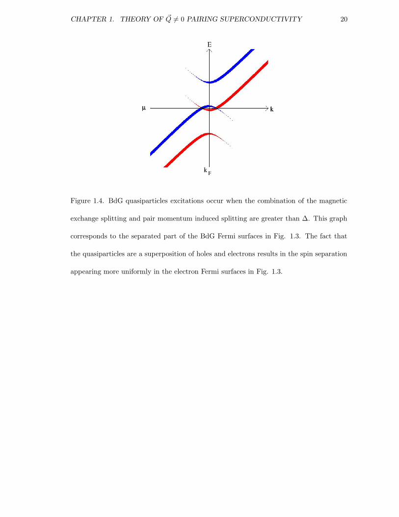
Figure 1.4. BdG quasiparticles excitations occur when the combination of the magnetic
exchange splitting and pair momentum induced splitting are greater than ∆. This graph
corresponds to the separated part of the BdG Fermi surfaces in Fig. 1.3. The fact that
the quasiparticles are a superposition of holes and electrons results in the spin separation
appearing more uniformly in the electron Fermi surfaces in Fig. 1.3.

CHAPTER 1. THEORY OF ~Q 6= 0 PAIRING SUPERCONDUCTIVITY 21
FFLO phases are favored when (1) enough of the Fermi surface can be paired
(nesting is strong enough) to allow for a superconducting (∆ 6= 0) solution to the gap
equation, (2) the FFLO free energy is less than the BCS free energy and normal param-
agnetic free energy. Using the form of the gap equation that includes the nesting density,
we want to understand what features of the Fermi surface favor the FFLO state. For a
given splitting and direction of q, the lowest FFLO free energy occurs when pairing is
maximized. Pairing is enhanced when 12qV = ~q
2 · ~v~kFis chosen to cancel the magnetic
splitting on some part of the Fermi surface. The value of q selects the range of V where
|12qV −B| < ∆ (e.g. where nesting occurs).
The effective width of nesting in V space can be found by noting when the
quasiparticle eigenenergies are greater than zero at the Fermi surface. Rewriting the
inequality as | 12q(V0 + δV ) −B| < ∆, we find
δV ≈ 2∆
q≈
∣
∣
∣
∣
V0∆
B
∣
∣
∣
∣
(1.29)
where V0 solves the equation | 12qV0 − B| = 0. In general, V0 will be optimal near a peak
in the nesting density and as large as possible to maximize δV .
Figure 1.5 illustrates the behavior of the energy integral K(∆, T, 12qV − B) for
two possible choices of q which solve the equation | 12qV0 − B| = 0 at different values of
V0, T = 0, and fixed ∆ < B. As long as ∆ > B − qV , the integral will be a constant
(≈ 0.4 in this case). For the q = 0 case, ∆ < B − 0V over the entire range causing pair
breaking over the entire Fermi surface. The figure also shows two possible values of pair
momentum. Plateaus occur when ∆ < B − qV causes both Fermi functions to be zero at

CHAPTER 1. THEORY OF ~Q 6= 0 PAIRING SUPERCONDUCTIVITY 22
the Fermi surface.
0
0.1
0.2
0.3
0.4
0.5
-1 -0.5 0 0.5 1
K(∆
,T,B
+qV
/2)
Reduced Velocity V/VMAX
Small qLarge q
BCS
Figure 1.5. Graph of the energy integral part of the gap equation (K(∆, T, 12qV − B))
as a function of V for two values of q, fixed ∆ and T = 0. The plateau occur where
the magnitude of the exchange splitting energy is less than ∆ since this is where both
Fermi functions are zero at the Fermi surface. The sharp drop at the edge of the plateau
reflects the breaking of pairs at the Fermi surface. Note how low values of q produce wider
plateaus at higher values of V .

CHAPTER 1. THEORY OF ~Q 6= 0 PAIRING SUPERCONDUCTIVITY 23
1.8 Applications of Nesting Density to FFLO calculations
For the calculations, we normalize ∆(B = 0, T = 0) = ∆0 = 1 to specify the
energy scale for the problem. The energy cutoff for the gap equation is a parameter
that is set to εc = 50∆0. In a real material the energy cutoff would be determined by
the pairing boson (phonon, spin fluctuation, etc.). With the above parameters set, the
coupling strength λ now becomes a function of εc and ∆0 , given by
1
λ= sinh−1
(
εc∆0
)
(1.30)
In the weak coupling regime (λ ≡ Nog << 1) this reduces to the well known BCS relation
∆0 = 2εce−1/λ. This coupling strength λ ≈ 0.2 for εc/δ0 = 50 is well within the weak
coupling regime for which the equations were derived.
The free energy competition between BCS and FFLO is a crucial factor in de-
termining whether an FFLO state will exist. Even in the best case, at T = 0 the free
energy driven transition from BCS to FFLO occurs very near the BCS critical field which
is proportional to the density of states at the Fermi surface. The FFLO critical field
calculation is more complex. A higher proportion of FFLO pairs occur in electron states
away from the Fermi surface and on average pay a higher kinetic energy cost. However to
first order the FFLO critical field is determined by the fraction of nesting density where
pairing occurs at the Fermi surface. If the FFLO critical field is less than the BCS critical
field for a material, no FFLO states will exist.

CHAPTER 1. THEORY OF ~Q 6= 0 PAIRING SUPERCONDUCTIVITY 24
1.9 1D Fermi Surface
The simplest case is the 1D Fermi surface. The nesting density consists of δ
functions at ±vF . The resulting phase diagram is given in Fig. 1.6. At T = 0, solutions
to the gap equation extend to arbitrarily large B with a correspondingly large q = 2B/vF .
Free energy constraints however limit the FFLO phase to finite B.
At the higher applied fields, the pairing on one half of the Fermi surface will be
almost completely suppressed and not contribute to the condensate. It may be possible
that a second condensate form that has opposite pair momentum.
0
0.5
1
1.5
2
2.5
3
0 0.1 0.2 0.3 0.4 0.5 0.6
Redu
ced
field
B/∆
0
Reduced Temperature T/∆0
FFLOBCS
Figure 1.6. The phase diagram of a 1D system. The presence of a δ function in the
nesting density guarantees that half the density of states at the Fermi surface can always
be paired.

CHAPTER 1. THEORY OF ~Q 6= 0 PAIRING SUPERCONDUCTIVITY 25
1.10 2D Fermi Surface
The nesting density of states for 2D Fermi surfaces will tend to have van Hove
like singularities, as observed by Shimahara [27], that produce strong peaks in N(V, q)
that go as 1/√
|Vpeak − V |. These peaks arise whenever V = q ·~vF is at a local extremum.
A simple example is the circular Fermi surface. The projected velocity is V = |vF |cos(φ)
where φ is the angle between ~vF and q. Figure 1.7 is the nesting density for positive V
and shows the peak caused by the extrema that occurs when q is normal to the Fermi
surface. Figure 1.8 shows the phase diagram for the circular Fermi surface. From Eq.
1.29, we know that as B is raised, the width of pairing (δV ) will go down. This happens
directly through the increase of q necessary to maintain V0 near the peak, and indirectly
through the reduction in ∆ caused by the decrease in pairing. This reduction in pairing
as B is raised causes the FFLO phase to be quenched much earlier than the 1D case.

CHAPTER 1. THEORY OF ~Q 6= 0 PAIRING SUPERCONDUCTIVITY 26
0
1
2
3
4
5
6
0 0.2 0.4 0.6 0.8 1 1.2N
(V,q
)
Reduced Velocity V/VMAX
Nesting Density
Figure 1.7. The nesting density of a 2D circular Fermi Surface for positive V showing
peak at V = |vF |. The optimal FFLO solution will chose a value for q such that this peak
has enhanced pairing. The nesting density is symmetric around V = 0 due to inversion
symmetry of the Fermi surface.
0
0.2
0.4
0.6
0.8
1
0 0.1 0.2 0.3 0.4 0.5 0.6
Redu
ced
field
B/∆
0
Reduced Temperature T/∆0
FFLOBCS
Figure 1.8. The phase diagram of a 2D circular Fermi Surface. The FFLO region is reduced
from the 1D case due to a lower percentage of states benefiting from the enhanced pairing.

CHAPTER 1. THEORY OF ~Q 6= 0 PAIRING SUPERCONDUCTIVITY 27
1.11 3D Fermi Surface
While the nesting density for 3D material may have peaks, in most cases these
peaks will not be caused by van Hove singularities. This can be understood by noting that
any extrema in the projected velocity will usually occur at isolated points on the Fermi
surface. For example on the spherical Fermi surface, the extrema of V occur at the two
points where q is normal to the Fermi surface. The nesting density for a spherical Fermi
surface is constant between ±|vF |, and consequently our calculations have shown a very
small FFLO region in the phase diagram.
A 3D example with a strong peak in the nesting density at Vmax is simple cubic
nearest neighbor tight binding model at half filling. With q taken in the 100 direction,
the projected velocity as a function of the position on the Fermi surface is given by
V = Vmaxsin(kx) (1.31)
where that lattice constant is assumed to be 1. V has extrema at kx = ±π/2 which occurs
along a curve defined by cos(ky) + cos(kz) = 0. Since extrema occur along a curve rather
than a point, N(V, q) will have integrable divergences that go as (|Vpeak−V |)−1/2. Figure
1.9 is the tight binding Fermi surface with the enhanced pairing region highlighted. The
nesting density is similar to that shown in Fig. 1.7 with slightly more weight in the peak.
Because of the increased weight, the resulting phase diagram seen in Fig. 1.10 shows an
increased FFLO region relative to the circular Fermi surface case. Any deviation from the
100 direction will cause the extrema in V to occur at a few isolated points.

CHAPTER 1. THEORY OF ~Q 6= 0 PAIRING SUPERCONDUCTIVITY 28
Figure 1.9. Tight binding Fermi surface at half filling. The white region corresponds to
the part of the Fermi surface where enhanced pairing occurs for T = 0, B ≈ 0.9, and
q along the 100 direction. Because the pairing is suppressed on the opposite side of the
Fermi surface, it conceivable that a separate condensate could form with q along the −100
direction.

CHAPTER 1. THEORY OF ~Q 6= 0 PAIRING SUPERCONDUCTIVITY 29
0
0.2
0.4
0.6
0.8
1
0 0.1 0.2 0.3 0.4 0.5 0.6
Redu
ced
field
B/∆
0
Reduced Temperature T/∆0
FFLOBCS
Figure 1.10. Phase diagram for the 3D nearest neighbor tight binding system shows a
larger FFLO region than the circular phase diagram 1.8. This reflects the fact that the
nesting density for the tight binding case has more weight near Vmax.
CHAPTER 1. THEORY OF ~Q 6= 0 PAIRING SUPERCONDUCTIVITY 30
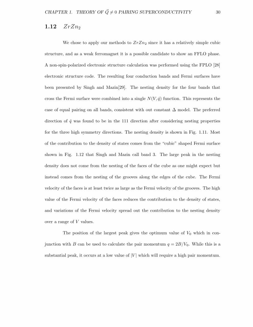
1.12 ZrZn2
We chose to apply our methods to ZrZn2 since it has a relatively simple cubic
structure, and as a weak ferromagnet it is a possible candidate to show an FFLO phase.
A non-spin-polarized electronic structure calculation was performed using the FPLO [28]
electronic structure code. The resulting four conduction bands and Fermi surfaces have
been presented by Singh and Mazin[29]. The nesting density for the four bands that
cross the Fermi surface were combined into a single N(V, q) function. This represents the
case of equal pairing on all bands, consistent with out constant ∆ model. The preferred
direction of q was found to be in the 111 direction after considering nesting properties
for the three high symmetry directions. The nesting density is shown in Fig. 1.11. Most
of the contribution to the density of states comes from the “cubic” shaped Fermi surface
shown in Fig. 1.12 that Singh and Mazin call band 3. The large peak in the nesting
density does not come from the nesting of the faces of the cube as one might expect but
instead comes from the nesting of the grooves along the edges of the cube. The Fermi
velocity of the faces is at least twice as large as the Fermi velocity of the grooves. The high
value of the Fermi velocity of the faces reduces the contribution to the density of states,
and variations of the Fermi velocity spread out the contribution to the nesting density
over a range of V values.
The position of the largest peak gives the optimum value of V0 which in con-
junction with B can be used to calculate the pair momentum q = 2B/V0. While this is a
substantial peak, it occurs at a low value of |V | which will require a high pair momentum.

CHAPTER 1. THEORY OF ~Q 6= 0 PAIRING SUPERCONDUCTIVITY 31
As was illustrated in Fig. 1.5, high pair momentum reduces the the amount of total den-
sity available for pairing. While FFLO solutions exist for the gap equation, at no point
was the free energy of these solutions below both the free energy for the BCS phase and
the normal phase.
By allowing a non-uniform ∆, it may be possible for FFLO solutions to exist in
a small region above the BCS phase, however other considerations make this unlikely. In
the Hamiltonian we have assumed, the Zeeman splitting term B for ferromagnets includes
the applied field as well as the ferromagnetic exchange energy. The average B for ZrZn2
can be calculated as
B =M
2N0≈ 30 meV (1.32)
where M ≈ 0.15µB and using the Singh and Mazin calculated value N0 = 2.43 states/eV -
spin-unit cell). Since the Curie temperature is greater than the observed superconducting
temperature, we are not able to determine ∆0 = ∆(T = 0, B = 0) for ZrZn2. We can
however place a lower bound on ∆0 for singlet pairing by noting that even allowing for
FFLO solutions, the maximum B will be on the order of ∆0/√
2. The resulting ∆0 is
orders of magnitude to large as it would correspond to a Tc ≈ 2∆0/3.52kB = 280K From
this we conclude that singlet pairing of either BCS or FFLO states is highly unlikely.

CHAPTER 1. THEORY OF ~Q 6= 0 PAIRING SUPERCONDUCTIVITY 32
0
0.25
0.5
0 4 8
N(V
,q)
V
All bands 111
Figure 1.11. ZrZn2 nesting density. The units of V are 107 cm/sec. A small non-zero
density extends to higher values of V . The noise is a function of both the finite sampling
of the Fermi surface and the complexity of the electronic structure.

CHAPTER 1. THEORY OF ~Q 6= 0 PAIRING SUPERCONDUCTIVITY 33
Figure 1.12. Fermi surface for the cube shaped band that is responsible for the peak in
the nesting density 1.11. The white region corresponds to the part of the Fermi surface
where enhanced pairing occurs for T = 0, B ≈ o.6, and q in the 111 direction. It is
interesting that the pairing is not favored on the relatively flat faces of the cube as one
might expect. These faces however have a non-uniform velocity distribution which makes
them less suitable for non-zero momentum pairing.

CHAPTER 1. THEORY OF ~Q 6= 0 PAIRING SUPERCONDUCTIVITY 34
Recent evidence has been presented that the superconductivity observed in sam-
ples of ZrZn2 is a surface phenomenon [30], consistent with the lack of any signal in the
heat capacity. The superconductive surface seems to be a product of sample manufacturing
and is eliminated by etching to produce a clean surface.
1.13 Conclusion
We have presented the formalism for the specific case of the quasiparticle states
and eigenenergies for non-zero momentum BdG quasiparticles in an exchange field. These
quasiparticles were then used to solve the superconducting gap equation within the mean
field approximation. The spin polarized BdG formalism was then applied to study FFLO
states which have magnetically induced spin splitting leading to pair momentum enhanced
superconducting pairing on a subset of the Fermi surface. The nesting density, which is
derived from the Fermi surface of the material being studied, was separated out and
calculated to facilitate solving the gap equation and calculating free energies and other
observables. In addition to providing an efficient means of performing calculations, the
nesting density also proved to be a useful tool for understanding what features of a Fermi
surface contribute to the formation of FFLO states.
The features of a Fermi surface which promote FFLO states are low dimen-
sionality, specific nesting topographies, (not necessarily like those that drive charge-and
spin-density waves) and relatively simple Fermi surfaces with uniform magnitude of the
Fermi velocity. The benefits of low dimensionality is demonstrated by circular vs. spher-

CHAPTER 1. THEORY OF ~Q 6= 0 PAIRING SUPERCONDUCTIVITY 35
ical Fermi surfaces. The tight binding Fermi surface illustrates the benefits of nesting
topographies. It is important to recognize that the nesting topography in this case is not
a “flat sheet” which we intuitively associate with nesting. The fact that FFLO states are
enhanced by peaks in the nesting density at high values of V is in conflict with the re-
duced density of states associated with high Fermi velocities. Variations in the magnitude
of the Fermi velocity will tend to place larger weights at small V which are less likely to
participate in FFLO pairing.
To simplify the calculations and analysis, we chose to consider only a uniform
exchange splitting which could arise from uniform ferromagnetic exchange field or from
an applied field. The BdG formalism does not depend on these assumptions and could be
applied to more complex situations that do not make use of a constant exchange splitting
and linearized Fermi surface approximation.
1.14 Free energy calculations
In all cases, the total energy of the system was taken to be relative to the ground
state of the normal metal at T = B = 0
Eg = 2∑
~k<~kF
ε~k (1.33)
With εc = 50 and [B, T,∆] ∼ 1 in units where ∆0 ≡ 1, excitations outside the cutoff can
be ignored. The free energy of the superconducting state when measured relative to the

CHAPTER 1. THEORY OF ~Q 6= 0 PAIRING SUPERCONDUCTIVITY 36
ground state becomes
Es − Eg =∑
|ε~k|<εc
(ε~k + w~k)(v2~kf(E−
~k↑) + u2
~kf(E+
~k↑))
+ (ε~k − w~k)(v2~kf(E−
~k↓) + u2
~kf(E+
~k↓))
+ (ε~k +q
2V~k)(Θ(ε~k +
q
2V~k) − 1)
+ (ε~k −q
2V~k)(Θ(ε~k −
q
2V~k) − 1)
− TS − ∆2
g(1.34)
The first two terms account for the kinetic energy of the electron part of the quasi particles.
The next two terms remove the kinetic energy for the ground state Eg. The last two terms
are respectively the entropy and pairing potential energy. In doing the calculation this
way, we have ignored the affect of the pairing energy q2V~k on the energy cutoff which
bounds the sum. With εc = 50 the impact is negligible, but for smaller cutoff energies it
becomes important.
1.15 Numerical methods
The first step in performing these calculations is to produce the nesting density
of states. This is accomplished by extracting a triangulation of the Fermi surface with
Fermi velocities from a dispersion relationship expressed on a grid. The nesting density
of states integral is converted to a sum and stored in a discrete histogram indexed by
V = q · ~v~kF
CHAPTER 1. THEORY OF ~Q 6= 0 PAIRING SUPERCONDUCTIVITY 37
N(V, q) =Ωc
(2π)3
∑
i
Areai~vFi
× Θ(1
2Vδ − |V − q · ~v~kF i
|) (1.35)
where Vδ is the projected velocity bin width, and i goes over all triangles. The preferred
direction for q can be found by looking for largest peaks at high V in the nesting density
calculated for each of the high symmetry directions.
There is a subtle danger associated with using discrete bins for the nesting density
for low temperatures and low ∆. The discrete bins will act like δ functions that will always
give a FFLO solution to the gap equation at high fields (see 1D Fermi surface section).
However, the temperature and ∆ of the possible solutions will go as exp(−1/N(Vδ)) which
will typically be on the order of e−10.
To determine the preferred state at a given temperature and applied field, it is
necessary to calculate the free energy for each possible state. Furthermore, the possible
superconducting states have ∆ and q degrees of freedom. Fortunately, the constraint set
by holding g constant means that we only need to search 1D isocontours in ∆-q space,
which we evaluate on a discrete grid. Finding this isocontour requires that that we perform
the integral in Eq. 1.26 many times.
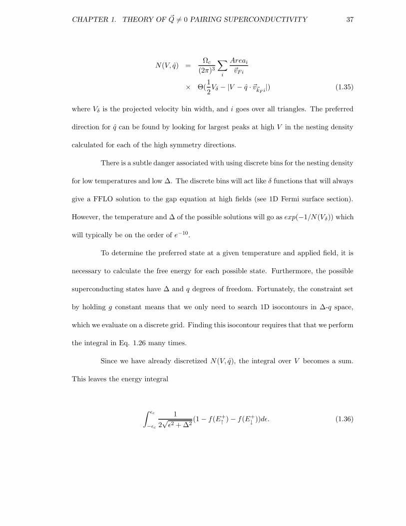
Since we have already discretized N(V, q), the integral over V becomes a sum.
This leaves the energy integral
∫ εc
−εc
1
2√ε2 + ∆2
(1 − f(E+↑ ) − f(E+
↓ ))dε. (1.36)

CHAPTER 1. THEORY OF ~Q 6= 0 PAIRING SUPERCONDUCTIVITY 38
This is a difficult integral to do numerically since it is highly peaked around ε = 0
and the behavior of the Fermi functions is highly temperature dependent. We chose to
take advantage of the fact that we know how to do part of the integral analytically.
∫
1
2√ε2 + ∆2
dε =1
2sinh−1(
εb∆
) (1.37)
This allows one to write formally
∫ εc
−εc
1
2(1 − f(E+
↑ ) − f(E+↓ ))d[sinh−1(
ε
∆)] (1.38)
This integral was discretized in a manner that allowed dealing with variations in
the Fermi functions. The numeric integral becomes
∑
εi
(1 − f(E+↑ ) − f(E+
↓ )) × (1.39)
[sinh−1(εi + εstep
∆) − sinh−1(
εi∆
)] (1.40)
with the variable step size
εstep ∝[
∂
∂ε(f(E+
↑ ) + f(E+↓ )) + δ
]−1
. (1.41)
The constant δ is needed to maintain a minimum step size. This variable step integration
is used in calculating contributions to the free energies and other observables of interest.

Chapter 2
Fermi Velocity and Incipient
Magnetism in TiBe2
39

CHAPTER 2. FERMI VELOCITY AND INCIPIENT MAGNETISM IN TIBE2 40
2.1 Introduction
The work in this chapter is derived from the publication
“Fermi velocity spectrum and incipient magnetism in TiBe2”; T. Jeong, A. B. Kyker, W.
E. Pickett, Phys. Rev. B 73, 115106 (2006).
The cubic Laves compound TiBe2 was already shown forty years ago to have quite
unusual behavior of the magnetic susceptibility χ(T ) and the Knight shift.[31] χ−1 showed
a strong increase with lowering temperature but a clear deviation from Curie-Weiss form,
while the Knight shift was temperature dependent and negative. The magnetic properties
of TiBe2 have been controversial since Matthias et al.[32] interpreted the susceptibility
peak at 10 K in TiBe2 as itinerant antiferromagnetism (AFM) with an associated mag-
netic moment of 1.64µB , and Stewart et al. reported a transition at 2 K that seemed
characteristic of magnetic ordering.
However, a clear picture has emerged gradually after the idea of weak itinerant
antiferromagnetism had been abandoned because of the subsequent lack of experimental
evidence[33, 34]. Many experiments have shown that TiBe2 is instead a strongly enhanced
paramagnet [35, 36, 37] and undergoes a metamagnetic transition[38, 39, 40] (field-driven
ferromagnetism) around 5.5 T. Also one can see similarity to the magnetic behavior of
Ni3Ga by comparing the values of the low temperature susceptibility, χ = 1.65 × 10⁻²
emu/mole for Ni3Ga[41] and χ = 0.90 × 10⁻² emu/mole for TiBe2[32]. Based on the
magnetization data of Monod et al[36] Wohlfarth[39] suggested the transition at 5.5 T
should be first order. Wohlfarth’s considerations received at least partial support from
CHAPTER 2. FERMI VELOCITY AND INCIPIENT MAGNETISM IN TIBE2 41
theoretical band-structure considerations coupled with the de Haas-van Alphen data of
van Deursen et al[42].
Clarity began to arise with the extensive experiments of Acker et al. who in-
terpreted their magnetization data[35] in fields to 21T and the magnetization data of
Monod et al. [36] as evidence for exchange-enhanced paramagnetism or spin fluctuations
in TiBe2. They found the system TiBe2−xCux to become FM at a critical concentration
xcr = 0.155. Stewart et al.[43] measured the specific heat of TiBe2 (γ = 42 mJ/mole
K2) at low temperature in 0 and 7T and interpreted the behavior as evidence of spin
fluctuations.
The isoelectronic isostructural material ZrZn2 is considered a classic example of
an weak itinerant ferromagnet. Magnetic measurements find very small magnetic moments
(values from 0.12 to 0.23 µB )[44, 45], hence the characterization as a weak ferromagnet.
The magnetization of ZrZn2 increases substantially with field, but unlike TiBe2 with its
metamagnetic transition, the increase continues smoothly to fields as high as 35 T. The
Curie temperature TC drops approximately linearly with pressure, from 29 K at P = 0 to
4K at P = 16 kbar, which extrapolates to a quantum critical point (QCP) at P = 18− 20
kbar. The report of superconductivity coexisting with ferromagnetism in ZrZn2 near this
QCP[46] enlivened both theoretical and experimental attention, but more recently it has
been shown[30] there is no bulk superconductivity. TiBe2, on the other hand, has been
nearly addressed only rarely for the past twenty years.
The complex temperature-field behavior of TiBe2 has led to many speculations
about the microscopic mechanisms. Of course spin fluctuations play a central part, and

CHAPTER 2. FERMI VELOCITY AND INCIPIENT MAGNETISM IN TIBE2 42
the highly enhanced susceptibility suggests this system is near a quantum critical point
(at slightly enlarged lattice constant, say, as well as for the Cu alloying). If FM fluc-
tuations dominate, then a metamagnetic transition (field-driven FM state) around 5 T
would make sense. If AFM fluctuations dominate, application of a field suppresses the
fluctuations, providing another way to interpret specific heat under applied field.[47] The
anomalies in the conduction electron spin resonance (CESR) linewidth[48] around 2 K
have been interpreted in terms of a thermal spontaneous magnetism,[49] and a decrease
in the resistivity is also seen at that temperature.[35] All of these scenarios are sensitive
to the Fermi surface shape, velocity spectrum, and possibly the energy dependence of the
density of states near the Fermi energy, and it is these questions that we address in this
paper.
Band structure intricacies by themselves also can come into play. Shimizu
showed[49] that an independent electron system with magnetic coupling can undergo
a first-order transition to a “spontaneous thermal magnetism” state (within a range
T1 < T < T2) if it is highly enhanced and if the Fermi level lies within a local minimum in
the density of states. The effects of magnetic fluctuations should of course be added[50]
to the free energy of both the ordered and disordered phases to make this treatment more
realistic.
Local density approximation (LDA) energy band studies of TiBe2 have been
reported previously [51, 52, 53]. Those studies revealed a split narrow peak in in the
density of states (DOS) N(E) near the Fermi energy (EF ), with calculated Stoner factors
IN(EF ) greater than unity, giving the Stoner instability to FM. Here I is the Stoner

CHAPTER 2. FERMI VELOCITY AND INCIPIENT MAGNETISM IN TIBE2 43
exchange interaction averaged over the Fermi surface. Thus, as for a few cases that have
come to light more recently,[54, 55] ferromagnetism is incorrectly predicted, indicating the
need to account for magnetic fluctuations not included in LDA that will suppress magnetic
ordering. By comparing the calculated value of N(EF ) with the measured susceptibility,
a Stoner enhancement S = [1 - IN(EF )]−1 ≈ 60 was obtained, making TiBe2 a more
strongly exchange enhanced metal than Pd.
All of these calculations, carried out 25 years ago, used shape approximations
for the density and potential, and for a detailed investigation of the weak ferromagnetism
precise electronic structure methods are required. In this work, the precise self-consistent
full potential linearized-augmented-plane-wave (FLAPW) method and full potential local
orbital minimum basis band structure scheme (FPLO) are employed to investigate thor-
oughly the electronic and magnetic properties of TiBe2 based on the density functional
theory. We compared and checked the calculation results of the both methods. We con-
sider the effect of magnetism on the band structure and Fermi surface, Fermi velocity and
compare with experiment and previous band calculations.
2.2 Crystal Structure
TiBe2 crystallizes into a cubic Laves phase C15 crystal structure. The C15 (AB2
) structure is a close packed structure and the site symmetry is high for the two con-
stituents. Ti atoms occupy the positions of a diamond sublattice while the Be atoms form
a network of interconnected tetrahedra, with two formula units per cell. Since the major

CHAPTER 2. FERMI VELOCITY AND INCIPIENT MAGNETISM IN TIBE2 44
contributions to N(EF ) come from Ti, the local environment of Ti atoms is particularly
important to keep in mind. Each Ti is surrounded by 12 Be neighbors at a distance of 2.66
A and tetrahedrally by four Ti neighbors a distance 2.78 A away. The TiBe2 structure
belongs to the Fd3m space group with Ti occupying the 8a site, and Be the 16d site.
The site symmetry of Ti is 43m(tetrahedral) and Be has 3m site symmetry. The atomic
positions are symmetry determined, and we used experimental lattice constant 6.426 A
for all calculations.
2.3 Method of Calculations
We have applied the full-potential nonorthogonal local-orbital minimum-basis
(FPLO) scheme within the local density approximation (LDA).[56] In these scalar relativis-
tic calculations we used the exchange and correlation potential of Perdew and Wang.[57]
Ti 3s, 3p, 4s, 4p, 3d states and Be 2s, 2p, 3d were included as valence states. All lower
states were treated as core states. We included the relatively extended semicore 3s, 3p
states of Ti as band states because of the considerable overlap of these states on nearest
neighbors. This overlap would be otherwise neglected in our FPLO scheme. Be 3d states
were added to increase the quality of the basis set. The spatial extension Of the basis
orbitals, controlled by a confining potential (r/r0)4, was optimized to minimize the total
energy.
The self-consistent potentials were carried out on a mesh of 50 k points in each
direction of the Brillouin zone, which corresponds to 3107 k points in the irreducible zone.

CHAPTER 2. FERMI VELOCITY AND INCIPIENT MAGNETISM IN TIBE2 45
A careful sampling of the Brillouin zone is necessary to account carefully for the fine
structures in the density of states near Fermi level EF . For the more delicate numerical
integrations, band energies were extracted from FPLO in an effective mesh of 360 k points
in each direction. A separate tool was developed to extract energy isosurfaces with gra-
dients from the scaler energy grid. The isosurfaces were then used to calculate density of
states and velocity moments.
To check carefully the fine structure that we will discuss, we also repeated sev-
eral calculations with the general potential linearized augmented plane wave (LAPW)
method,[29] as implemented in the WIEN2K code.[58] Relativistic effects were included
at the scalar relativistic level. However, we verified that the magnetic moment with
the experimental structure is not sensitive to the inclusion of the spin-orbit interaction.
For the generalized gradient approximation (GGA) calculations, we used the exchange-
correlation functional of Perdew, Burke, and Ernzerhof. [59] We choose the muffin-tin
spheres RMT = 2.6 a.u. for Ti, RMT = 2.1 a.u. for Be and a basis set determined by a
plane-wave cutoff of RMTKmax = 7.0, which gives good convergence. The Brillouin zone
samplings were done using the special k point method with 1280 points in the irreducible
zone.
2.4 Results and Discussions
For orientation we first show the full nonmagnetic band structure of TiBe2 in
Fig. 2.1, which is consistent with earlier calculations of [51, 52, 53]. The Be 2s bands

CHAPTER 2. FERMI VELOCITY AND INCIPIENT MAGNETISM IN TIBE2 46
Figure 2.1. The full LDA band structure of non-magnetic TiBe2 along symmetry lines
showing that there are several bands near the Fermi level (taken as the zero of energy)
with weak dispersion; they are primarily Ti 3d in character.

CHAPTER 2. FERMI VELOCITY AND INCIPIENT MAGNETISM IN TIBE2 47
Figure 2.2. Band structure of non-magnetic TiBe2 of Fig. 2.1 on an expanded scale near
Fermi level. The flat bands along L-W-U/K-L lines (the hexagonal face of the fcc Brillouin
zone) give rise to the density of states structure discussed in the text.

CHAPTER 2. FERMI VELOCITY AND INCIPIENT MAGNETISM IN TIBE2 48
Figure 2.3. The total and atom-projected density of states (Ti, short dashed line; Be, the
lower, long dashed line) for non-magnetic TiBe2 per primitive cell. The inset gives the
density of states for the ferromagnetic TiBe2 showing the exchange splitting 0.6 eV. The
peak of the DOS for the majority spin is entirely below the Fermi level while that of the
minority spin is above the Fermi level.

CHAPTER 2. FERMI VELOCITY AND INCIPIENT MAGNETISM IN TIBE2 49
Figure 2.4. Fermi surfaces, top left: band 14, X-centered pillows; top right: band 15,
primarily X-centered jungle gym; bottom left: band 16, Γ-centered pseudocube; bottom
right: band 17, Γ-centered sphere. Fermi velocities colored dark (red) for lowest to lighter
(blue) for highest. Magnitudes of velocities are discussed in Sec. IV.A.

CHAPTER 2. FERMI VELOCITY AND INCIPIENT MAGNETISM IN TIBE2 50
lie between -8 eV and -2 eV. Above them the bands are of mixed s, p character, centered
on the Be as well as the Ti site. Near the Fermi level there are several bands with weak
dispersion, being of primarily Ti 3d character. The bands at K and L are hybridized
strongly, while at X the s, p character is the main character. As noted also by Jarlborg
and Freeman,[51, 52] one band at L falls extremely close to EF (3 meV below). This band
is doubly degenerate along Γ-L, and the L point forms the maximum of band 15 and a
saddle point for band 16. As the Fermi energy rises (for added electrons, say) the Fermi
surface sweeps through the L point saddle, where the band has a vanishing velocity by
symmetry. This vanishing velocity is discussed below. There is another doubly degenerate
band very near Ef at the W point.
The density of states (DOS) is shown near EF in Fig. 2.3. The Fermi energy
EF falls extremely close to the edge of a very narrow peak in the DOS. The DOS peak
arises from Ti d bands hybridized with Be p states. Flat bands close to Fermi level cen-
tered mostly in regions near the L-W-U and W-K directions, i.e. the hexagonal faces
of the Brillouin zone, cause the sharp peak. Stewart et al.[43] measured the linear spe-
cific heat coefficient for TiBe2 of γ=42 mJ/K2 mole-formula unit. The calculated value
of N(EF )=5.33 states/eV/f.u. for TiBe2 corresponds to a bare value γo=12.6 mJ/K2
mole(formula unit), leading to a thermal mass enhancement 1+λ=3.3, or λ=2.3 arising
from phonons, magnetic fluctuations, and Coulomb interactions.
Density functional calculations are usually reliable in calculating the instability
CHAPTER 2. FERMI VELOCITY AND INCIPIENT MAGNETISM IN TIBE2 51
to ferromagnetism. The enhanced susceptibility[60] is given by
χ(T ) =χ0
1 −N(EF )I≡ Sχ0. (2.1)
where χ0 = µ2BN(EF ) is the bare susceptibility obtained directly from the band structure
and I is the Stoner exchange interaction constant. Here N(EF ) refers to both spins, and
hence forward we quote susceptibility in units where µB ≡ 1. The calculation of I is from
fixed spin moment calculations[61], in which the energy E(m) is calculated subject to the
moment being constrained to be m. The behavior at small m is E(m) = (1/2)χ−1m2 from
which I = 0.22 eV can be extracted from Eq. 2.1. This value of I gives IN(EF ) = 1.2,
larger than unity and very close to that calculated earlier,[52] corresponding to a Stoner
ferromagnetic instability.
As for a few other compounds, TiBe2 is incorrectly predicted by LDA to be
ferromagnetic. Since spin-orbit coupling is small in 3d magnets, we neglect it, so the di-
rection of magnetic polarization is not coupled to the lattice. We have calculated a consis-
tent magnetic moment for TiBe2: 0.97µB/f.u.(FPLO, LDA), 1.00µB/f.u.(LAPW, LDA),
1.10µB/f.u.(LAPW, GGA). This value is considerably larger than an earlier calculation[51]
(which also reported a much smaller value for ZrZn2 than obtained from more recent
calculations[62]). We address the overestimate of the tendency to magnetism below.
2.4.1 Fermi Surface and Fermi Velocity
In Fig. 2.4 we show the nonmagnetic Fermi surfaces shaded by the Fermi veloc-
ities. The position of EF near L and W points sensitively determine the exact shape of

CHAPTER 2. FERMI VELOCITY AND INCIPIENT MAGNETISM IN TIBE2 52
some Fermi surfaces. The shapes can be characterized as (a) small Γ-centered electron
sphere from band 17, (b) large Γ-centered electron pseudocube from band 16, (c) multiply
connected surface mostly enclosing holes around the X point from band 15, which we refer
to as the jungle gym, and (d) flat hole pillows centered at each of the three X points. The
doubly degenerate bands crossing EF along Γ-X and X-W guarantee touching of certain
surfaces along these lines.
The DOS peak at and above EF is due to the band near the L point where the
cube-shaped surfaces are about to form bridging necks. Figure 2.5 shows how the Fermi
velocity spectrum (N(V ;E)) changes with energy at the peak just above EF , at EF , and
at the first minimum below EF . The Fermi velocity spectrum is defined as
N(V ;E) =∑
~k
δ(E~k −E)δ(V~k − V ) (2.2)
=
∫
L(V ;E)
dLk|~vk ×∇k|~vk||
,
with normalization∫
N(V ;E)dV = N(E). Here L(V ;E) is the line of intersection of the
constant energy Ek = E surface with the constant velocity surface |~vk| = V . The gradient
of the velocity in the denominator makes this distribution delicate to calculate accurately.
N(E, V ) was calculated numerically by extracting a triangulated energy isosurface from
the band structure, then obtaining a velocity histogram of the states associated with the
isosurface.
The spectrum in Fig. 2.5 shows, at EF , velocities extending down to the very
low value of 2×106 cm/s, and up to 5×107 cm/s, a variation of a factor of 25. Roughly
half of the weight lies below 107 cm/s. At the van Hove singularity at +3 meV, the only

CHAPTER 2. FERMI VELOCITY AND INCIPIENT MAGNETISM IN TIBE2 53
Figure 2.5. Fermi velocity spectrum of TiBe2. The low Fermi velocity states are the
primary source of changes to the density of states.
noticeable difference is additional velocities extending down to zero due to the vanishing
velocity at L (we have not worried about reproducing the V → 0 behavior precisely). At
-25 meV, which is just below the narrow peak at EF , the strong weight in the spectrum
appears only at 7×106 cm/s. Note that there is very little change in the high velocity
spectrum over small changes in energy.
2.5 Analysis of Velocity Distribution and Susceptibility
2.5.1 Renormalization due to Spin Fluctuations
Following the work of Larson, Mazin, and Singh[63] for Pd which builds on
Moriya theory, we first attempted to identify the relevant band characteristics in order to

CHAPTER 2. FERMI VELOCITY AND INCIPIENT MAGNETISM IN TIBE2 54
Figure 2.6. Top panel: < 1v(E) > plotted versus energy, showing the square root divergence
of the inverse moment of velocity near the Fermi energy. Unit conversion is: 1 eV Bohr =
8×106 cm/s. Bottom panel: the graph of the second moment of velocity (with constants
included to show it as the square of the Drude plasma energy) is concave downward, which
gives rise to the negative value of the Moriya A parameter. This sign of A is verified by
the calculation of χ(q) at small q (see text).

CHAPTER 2. FERMI VELOCITY AND INCIPIENT MAGNETISM IN TIBE2 55
evaluate the spin fluctuation reduction of χ in TiBe2. For this, one begins with the bare
susceptibility in the small q and small ω limit, given by
χ0(~q, ω) = N(EF )[1 −A(qa
2π)2 + i
1
2<
1
v>F
ω
q], (2.3)
while the screened susceptibility using the RPA approximation is given by
χ−1(~q, ω) = χ−10 (~q, ω) − I. (2.4)
The Moriya parameter A = −1.8, expressed in dimensionless form here, and mean inverse
Fermi velocity < 1/v >F≡ v−1F (the second Moriya parameter, discussed below) are derived
from velocity moments and DOS of the band structure, and like the density of states, they
are greatly influenced by the Fermi surface topology and its velocity spectrum. Specifically,
changes in topology which give rise to points of zero velocity in the band structure near
the Fermi surface become an important factor. The mean inverse Fermi velocity which
governs the imaginary part of χ0(~q, ω) is given by
<1
v(E)>≡ v−1(E) =
∑
k
δ(εk −E)
|~vk|/∑
k
δ(εk −E) (2.5)
evaluated at EF . The difference between < v−1 >F and 1/< v >F is one measure of the
velocity variation of the Fermi surface. The bottom or top of a three-dimensional band
(corresponding to the appearance or vanishing of a Fermi surface) gives only a discontinuity
proportional to the square of the band mass. At a saddle point, such as the merging of
the corners of the pseudocube Fermi surfaces, v−1(E) undergoes a 1/√E −Ecr divergence
because the associated Fermi surface area does not vanish. This “van Hove singularity” in
v−1(E) is evident for the band edge 3 meV from EF in TiBe2 in Fig. 2.6. We calculated
1/v−1F = 5 × 106 cm/s for TiBe2.
CHAPTER 2. FERMI VELOCITY AND INCIPIENT MAGNETISM IN TIBE2 56
For cubic structures, the parameter A in Eq. 2.3 is given by
A =1
48πe2(2π
a)2d2Ω2
p(EF )
dE2F
(2.6)
Ω2p(EF ) =
4πe2
3
∑
k
~v2kδ(εk −EF )
≡ 4πe2
3N(EF )v2
F .
Thus A it is proportional to the second derivative of the square of the Drude plasma
energy Ωp (i.e. ~ is absorbed into Ωp, so Ωp here explicitly has energy units; k sums
are understood to be normalized over the zone). The second moment of velocity is finite
everywhere, but its second derivative is not (for example, for free electrons this diverges as
the band edge). Derivatives have the unfortunate property of amplifying noise in numerical
evaluations. We have addressed the noise issue by using a large number of k points in the
numerical integration (360× 360× 360). By fitting Ωp(E)2 with a polynomial near the
Fermi energy, we obtain the above-mentioned value A = −1.8. The Fermi velocity was
calculated to be vF = 2.3 eV bohr = 1.8 ×107 cm/s.
2.5.2 q-dependent Susceptibility
The negative value of the A parameter indicates, from Eq. 2.3, that the primary
magnetic instability in TiBe2 does not lie at q=0 but rather at finite q, so it is more
susceptible to AF instability (including possibly a spin spiral) rather than ferromagnetic.
The sign of A has been verified independently by explicit calculation of the real part of
χ(~q), with results shown in Fig. 2.7.
The calculation of χα,β(~q) between bands α and β was performed by an isosurface

CHAPTER 2. FERMI VELOCITY AND INCIPIENT MAGNETISM IN TIBE2 57
Figure 2.7. Intraband contribution to the real part of χ(~q). The increase at small q
confirms the sign of Moriya A coefficient (see text). Although both [110] and [111] direc-
tions have a maximum at the zone boundary, the peak along [100] (X point of the zone)
dominates the instability.

CHAPTER 2. FERMI VELOCITY AND INCIPIENT MAGNETISM IN TIBE2 58
slicing method. The susceptibility can be written, after inserting a factor 1 ≡∫
d∆ δ(∆−
εβ,~k+~q
+ εα,~k
), as
χαβ(~q) =
∫
d∆Nχαβ(∆)
∆, (2.7)
Nχαβ(∆) =
∑
k
[f(εα,~k
) − f(εβ,~k+~q
)]δ(∆ − εβ,~k+~q
+ εα,~k
),
where Nχαβ(∆) is a susceptibility density calculated from the isosurface defined by the
Fermi functions and the energy δ function. The Brillouin zone was divided into a 140 ×
140 × 140 grid of cubes. Within each cube the ∆ integral is calculated as a discrete sum,
using variable step sizes in ∆ corresponding to 1/30 of the maximum difference in energies
εβ,~k+~q
+ εα,~k
within the cube.
The susceptibility rises equally along all three symmetry directions (as required
by cubic symmetry), but only for q along the cubic axis does χ(~q) continue to increase
strongly beyond the small-q region. The maximum of χo(~q) occurs at the X point, where
the intraband part has increased by nearly 50% over its q=0 value. In such cases where
q=0 is not the maximum, it is necessary to apply the extension of weak ferromagnets to
the AF case.[64]
The band-by-band contributions to χo(q) have been evaluated both to verify the
code and to identify the source of the important contributions and structures. The sphere
FS gives rise to a Lindhard type form with 2kF ≈ π/a (but is not perfectly round). The
pillows lead to a cusp for (qx, 0, 0) for qx ≈ 0.28π/a, and along all three directions decreases
for q ≥ π/a. For the jungle gym and the pseudocube,χ increases by a factor of two at the
zone boundary along (qx, 0, 0), with much less variation in the other two directions. The
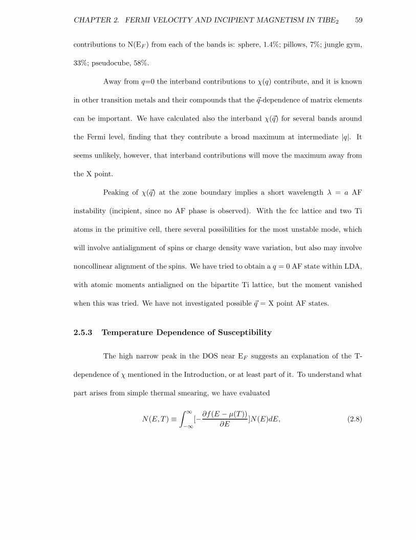
CHAPTER 2. FERMI VELOCITY AND INCIPIENT MAGNETISM IN TIBE2 59
contributions to N(EF ) from each of the bands is: sphere, 1.4%; pillows, 7%; jungle gym,
33%; pseudocube, 58%.
Away from q=0 the interband contributions to χ(q) contribute, and it is known
in other transition metals and their compounds that the ~q-dependence of matrix elements
can be important. We have calculated also the interband χ(~q) for several bands around
the Fermi level, finding that they contribute a broad maximum at intermediate |q|. It
seems unlikely, however, that interband contributions will move the maximum away from
the X point.
Peaking of χ(~q) at the zone boundary implies a short wavelength λ = a AF
instability (incipient, since no AF phase is observed). With the fcc lattice and two Ti
atoms in the primitive cell, there several possibilities for the most unstable mode, which
will involve antialignment of spins or charge density wave variation, but also may involve
noncollinear alignment of the spins. We have tried to obtain a q = 0 AF state within LDA,
with atomic moments antialigned on the bipartite Ti lattice, but the moment vanished
when this was tried. We have not investigated possible ~q = X point AF states.
2.5.3 Temperature Dependence of Susceptibility
The high narrow peak in the DOS near EF suggests an explanation of the T-
dependence of χ mentioned in the Introduction, or at least part of it. To understand what
part arises from simple thermal smearing, we have evaluated
N(E, T ) ≡∫ ∞
−∞[−∂f(E − µ(T ))
∂E]N(E)dE, (2.8)

CHAPTER 2. FERMI VELOCITY AND INCIPIENT MAGNETISM IN TIBE2 60
where the chemical potential µ(T ) is adjusted at each temperature to keep the number
of electrons (occupied states) constant. The result is shown as a series of curves for T
ranging from zero to 300 K. It is necessary to include the variation in µ, and the value of
N(µ(T ), T ) decreases by 8%.
The resulting change in the physical, enhanced susceptibility is given by
χ(T ) =N(µ(T );T )
1 − IN(µ(T );T ). (2.9)
Adjusting I to reproduce the peak height (at 10 K, experimentally), which requires I=0.183
eV (S=56 at the maximum of N(µ)), the resulting enhanced χ(T ) is compared with the
data in the lower panel of Fig. 2.8. It is evident that this simple temperature smearing
accounts for much of the observed temperature dependence. Additional indirect temper-
ature smearing will come from phonons and from electronic and magnetic interactions as
these excitations are increasingly excited upon raising the temperature. We conclude that
TiBe2 contains no appreciable contribution to the susceptibility from local moments.
2.5.4 Field Dependence of Susceptibility
For an energy-dependent DOS and a highly enhanced susceptibility, a field-
dependent susceptibility χ(H,T = 0) ≡ χ(H) is expected. In TiBe2 a strong effect of
this kind has been seen, which can be characterized as field-driven ferromagnetism. The
differential susceptibility χd(H) = dM(H)/dH where M is given by the difference in elec-
tron occupations nσ(H). A many-body treatment shows that the spin imbalance can be
expressed[66] in terms of the spin-dependent thermal (energy E surface averaged) Green’s
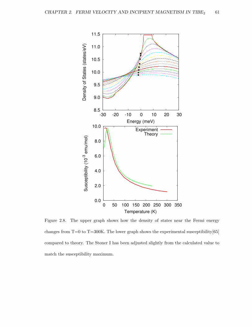
CHAPTER 2. FERMI VELOCITY AND INCIPIENT MAGNETISM IN TIBE2 61
Figure 2.8. The upper graph shows how the density of states near the Fermi energy
changes from T=0 to T=300K. The lower graph shows the experimental susceptibility[65]
compared to theory. The Stoner I has been adjusted slightly from the calculated value to
match the susceptibility maximum.

CHAPTER 2. FERMI VELOCITY AND INCIPIENT MAGNETISM IN TIBE2 62
Figure 2.9. Magnetic field (H) dependence of the Fermi level density of states for TiBe2,
referred to its H=0 value, as defined in the text. The initial increase with field indicates
an increasing instability towards ferromagnetic order.

CHAPTER 2. FERMI VELOCITY AND INCIPIENT MAGNETISM IN TIBE2 63
function
Gσ(E, iωn;H) =1
iωn − (E − µ− σµBH) − Σσ(H), (2.10)
nσ(H) =
∫
dEN(E)T∑
i
Gσ(E, iωn;H)eiωnη,
here ωn is the fermionic Matsubara discrete energy variable and η is a positive infinitesimal.
The simplest form of (Stoner) self-energy Σσ = σKµBH should be appropriate (1 +K =
S).
Taking the field derivative of M(H) but keeping H finite, and using (in this
approximation)
Gσ(E, iωn;H) = G(E − σµB(1 +K)H, iωn;H = 0) (2.11)
we obtain the result at zero temperature
χd(H) =dM(H)
d(µBH)(2.12)
= S[
N(EF − SµBH) +N(EF + SµBH)]
.
This clearly reduces to the usual T=0 result at H=0. A slightly better treatment would
have also some H-dependence of S due to the structure in N(E) and the delicate situation
here that IN(EF ) is approaching unity, but at this point we neglect such details.
The result for the relative correction
R =N(EF − SµBH) +N(EF + SµBH)
2N(EF )(2.13)
is shown in Fig. 2.9. The effect on the ratio (thus on the differential susceptibility) is clear,
however even with the factor of S=60 enhancement of the energy scale (µBH → SµBH)

CHAPTER 2. FERMI VELOCITY AND INCIPIENT MAGNETISM IN TIBE2 64
the peak occurs at a field one order of magnitude smaller than seen in experiment. This
difference seems to indicate that the field influence on the spin fluctuations dominates;
however the variation in N(E) will need to be accounted for in any quantitative explana-
tion.
2.6 Summary
The complex and sometimes confusing data on the enhanced paramagnet were
discussed in the Introduction. It seems clear that magnetic fluctuations will be required to
understand the underlying mechanisms. Here we have presented a precise calculation and
analysis of the electronic structure, especially focusing on the Fermi surfaces and velocity
spectrum at and near the Fermi level that underlies not only the single particle excitations
but also the spectrum of magnetic fluctuation in the itinerant limit, which clearly seems
to be the case in TiBe2.
Our calculations have confirmed the sharp structure in the density of states
around the Fermi level that had been noted earlier, and quantified the tiny energy scale
that is involved: the Fermi level lies in a region of steep DOS, just 3 meV from an abrupt
van Hove singularity. This singularity is derived from a doubly degenerate band at the L
point of the zone. We have shown how to calculated the spectrum of velocities (speeds)
over the Fermi surface, and find the spectrum to be peaked at (the low value of) 107 cm/s,
with much of the weight below that value. Moriya theory for weak ferromagnets requires,
for the imaginary part of the inverse susceptibility, the moment < 1/vF >; we have

CHAPTER 2. FERMI VELOCITY AND INCIPIENT MAGNETISM IN TIBE2 65
illustrated that 1/v(E) diverges at the van Hove singularity signaling possible problems
with applying Moriya theory to TiBe2.
Moriya theory for weak ferromagnets also requires the dimensionless quantity
A ∝ d2Ωp(E)/dE2 at the Fermi energy, where Ωp is the conventional transport Drude
energy. We find that this quantity is not positive, as it must be for an incipient ferromag-
net; rather it is negative indicating the dominating (nearby) magnetic instability is finite
q: antiferromagnetic, spin wave, spin spiral, etc. Direct calculation of the generalized
susceptibility χo(q) confirms the sign of A, and reveals the dominant instability to lie at
the X point of the Brillouin zone, making TiBe2 an incipient antiferromagnet.
We have shown that the sharp structure in N(E) has other consequences. First,
it leads to a T-dependent chemical potential. Together with the temperature broadening
of N(E) and the Stoner enhancement S ≈ 60, this simple temperature broadening can
account for most if not all of the temperature dependence of the susceptibility, which
some investigators had interpreted as Curie-Weiss-like. As a result, the occurrence of local
moments in TiBe2 can be ruled out. Similarly, we have shown that this sharp structure in
N(E), again together with the large Stoner enhancement, has a substantial effect on the
field-dependence of the differential susceptibility. There is still the question of how much
of the measured field dependence is due to this induced exchange splitting, and how much
is due to the effect of the field on the magnetic fluctuations.
Many of the results we have obtained here are strongly dependent on details of the
band structure and the position of the Fermi level. That these results reflect realistically
the mechanisms underlying the many fascinating observations obviously requires that the

CHAPTER 2. FERMI VELOCITY AND INCIPIENT MAGNETISM IN TIBE2 66
band structure formalism is applicable in detail to such systems and that the calculations
are accurate. Another requirement is that of high sample quality, that the stoichiometry
is precise and that defect concentration must be very low (simple impurity broadening
will affect behavior). These questions must be addressed in deciding whether to press
onward to a more complete and more challenging explanation that includes effects of both
magnetic fluctuations and the energy dependence of the density of states.

Chapter 3
Macroscopic Theory of Multi
Order Parameter Pairing in
Superconductiity
67

CHAPTER 3. MACROSCOPIC THEORY OF MULTI ORDER PARAMETER PAIRING IN SUPERCONDUCTIITY68
3.1 Multi Order Parameter Landau Theory
The Ginzburg-Landau theory has been a very successful phenomenological model
for describing orbital effects of superconductors. The theory correctly captures many of the
observed phenomena associated with the superconducting state including zero-resistance,
the Meissner effect, the Abrikosov vortex and vortex lattice arrangement, penetration
depth, coherence length, etc.
The Ginzburg-Landau generic theory is based on Landau’s generic theory of
second order phase transitions. Landau assumed that the free energy of a system is an
analytic function which shares the symmetry of the Hamiltonian, and a second order phase
transition occurs when a symmetry of the system is spontaneously broken. The free energy
density is written as
F = FN + FL(m) (3.1)
where FN is the normal free energy density and FL is the condensate free energy density.
An order parameter is introduced which is usually indicates the condensate density and
how the condensate breaks the symmetry. FL is Taylor expanded in terms of the order
parameter. In general, the order parameter has the dimension and field of the broken
symmetry, for brevity however I will only considering the breaking of a one dimensional
real symmetry such as a classical Ising model with no applied field. Taking the first two
non-zero terms, the Taylor expansion of FL becomes
FL(m) = αm2 +1
2βm4 (3.2)

CHAPTER 3. MACROSCOPIC THEORY OF MULTI ORDER PARAMETER PAIRING IN SUPERCONDUCTIITY69
where m is the order parameter representing the magnetization. Since the sign of m is
a symmetry of the Hamiltonian, only even powers are included in the Taylor expansion.
As long as m = 0 the system state also has inversion symmetry. As soon as m takes on
a finite value, it will have a definite sign and the inversion symmetry of the state will be
broken.
Assuming the axiom that the system will assume the state that minimizes the
free energy and that the order parameter is bounded, one must assume that β is greater
than zero. If α is also greater than zero, m = 0 minimizes FL(m). If α is less than zero,
the optimal value of m is found to be
m = ±√
−αβ
(3.3)
by minimizing FL(m) with respect to m2. Thus the phase transition occurs when α
changes sign. α is normally taken to be a function of temperature expanded around the
critical temperature
α = C(T − Tc) (3.4)
where C = dα/dT evaluated at Tc.
In general, a system may have many order parameters which may be coupled by
the Hamiltonian. For example consider two coupled Ising systems with order parameters
m1 and m2 which might be used to model two magnetic domains with some interaction.
The free energy density is
F = FN + FL (3.5)
FL = FL1(m1) + FL2(m2) + FL12(m1,m2) (3.6)

CHAPTER 3. MACROSCOPIC THEORY OF MULTI ORDER PARAMETER PAIRING IN SUPERCONDUCTIITY70
The FL1(m1) and FL2(m2) contributions are still restricted to even powers. The FL12(m1,m2)
may have odd powers as long as all terms are zero when m1 and m2 are zero. I will only
consider two terms: bi-quadratic and bi-linear. The Taylor expansion becomes
FL = α1m21 +
1
2β1m
41 + α2m
22 +
1
2β2m
42
+ Dm21m
22 + Jm1m2 (3.7)
Initially at high temperatures when both order parameters are zero, there are
two symmetries of the Hamiltonian to be broken. The breaking of these symmetries could
result in one phase transition, or two phase transitions.
Assuming that Tc1 6= Tc2 and J = 0, the bi-quadratic coefficient D will not
change the upper critical temperature. The lower critical temperature will be raised or
lowered depending depending on the sign of D. To maintain the finite values of the order
parameters at the energy minimum, D must be bounded in the negative direction by
D > −√
β1β2 (3.8)
A sufficiently large positive value of D will reduce the lower critical temperature to zero,
eliminating the second phase transition entirely.
Assuming that Tc1 6= Tc2 and D = 0, the bilinear coefficient J will always raise
the upper critical temperature. The new upper critical temperature occurs when the
following equality is satisfied
J2 = α1α2 (3.9)
with both α1 and α2 positive. Below the new upper critical temperature, both symmetries

CHAPTER 3. MACROSCOPIC THEORY OF MULTI ORDER PARAMETER PAIRING IN SUPERCONDUCTIITY71
are broken in a single phase transition.

CHAPTER 3. MACROSCOPIC THEORY OF MULTI ORDER PARAMETER PAIRING IN SUPERCONDUCTIITY72
3.2 Ginzburg-Landau Theory
An early attempt at a phenomenological description of the interaction of mag-
netism and superconductivity was developed by F. London. The London equation [22]
~Js = − m∗
n∗se∗2~A (3.10)
can be derived by applying the quantum mechanical current operator to a condensate
with a fixed phase and magnitude over a macroscopic region. This fixed phase can be
thought of as breaking a phase symmetry of the Hamiltonian. This differs from the non-
condensate where the electron phases are uncorrelated. By assuming a specific gauge
for ~A, the equation captures the observed phenomena of the Meissner effect including a
finite penetration depth. It however does not address the upper critical field. Even more
disturbing, it only works for one choice of the ~A gauge.
The Ginzburg-Landau theory of superfluid condensates [67] assumes a complex
condensate wave function
Ψ(~r) = |Ψ(~r)|eiθ(~r) (3.11)
to be used as the order parameter in a Landau second order treatment. Assuming a
complex field for the order parameter allowed for a quantum mechanical kinetic energy
term to be added to the free energy density. This kinetic energy term has the property
of coupling the supercurrents to the ~A field, as in the London equation, and placing an
energy cost on the supercurrents that must be balanced by the energy lowering of the
condensate.

CHAPTER 3. MACROSCOPIC THEORY OF MULTI ORDER PARAMETER PAIRING IN SUPERCONDUCTIITY73
Assuming that carriers are pairs and including a term for the magnetic energy,
the Ginzburg-Landau free energy density is
F = FN + α|Ψ|2 +1
2β|Ψ|4 +
1
4m|(−i~∇ + 2z ~A)Ψ|2 +
B2
2µ0(3.12)
where m and z are the mass and charge of an unpaired carrier. The condensate density is
given by |Ψ2|. The order parameter Ψ, the magnetic field and the condensate coefficients
may be spatially dependent. Even though the phase of θ(~r) is not fixed, θ(~r) for a con-
nected condensate is completely defined by the density and current up to a global phase
factor.
The Ginzburg-Landau non-linear partial differential equations are derived by
minimizing the free energy using the Euler-Lagrange method. Minimizing with respect to
the vector potential gives the differential equation
δF
δ ~A(~r)= ~RA =
iz~
2m(Ψ∗∇Ψ − Ψ∇Ψ∗) +
2z2
m|Ψ|2 ~A+
∇2 ~A−∇ · ~Aµ0
(3.13)
Minimizing with respect to the order parameters gives
δF
δψ(~r)= RΨ = αΨ + β|Ψ|2Ψ +
1
4m(−i~∇ + 2z ~A)2Ψ (3.14)
It is customary to assume a gauge where ∇· ~A = 0, but numerically this can be inconvenient
to maintain. In the absence of applied currents or electric potentials, ~RA and RΨ will
be zero at a local maximum or minimum of the energy. In time dependant Ginzburg
Landau theory [68][69], ~RA and RΨ will be proportional to the time derivative of ~A and
Ψ respectively. Because the Ginzburg-Landau equations are non-linear, solutions are not
guaranteed to be unique. This can easily be demonstrated by noting that Ψ = 0 and

CHAPTER 3. MACROSCOPIC THEORY OF MULTI ORDER PARAMETER PAIRING IN SUPERCONDUCTIITY74
∇×∇× ~A = 0 will always be a solution even when the energy can be lowered by forming
a condensate. The number of stationary points is greatly increased when the possibility
of vortex trapping and pinning is considered. In the numerical simulations, ~RA and RΨ
will be used as a residue and and may be modified to enforce boundary conditions.
Because the Ginsburg-Landau equations are a phenomenological theory, the co-
efficients α and β are used as material fitting parameters to match the penetration depth
(ξGL) and coherence length (λGL).
A magnetic field experiences an exponential decay as it penetrates into a super-
conducting half space. If one assumes a fixed condensate density defined by the equilibrium
value ns = −β/α when α < 0, the penetration depth is found from the vector GL equation
to be
λGL =
√
m
2µ0e2ns=
√
−βm2µ0e2α
(3.15)
which matches the London result.
The coherence length is characterized by a competition between the kinetic en-
ergy and potential energy as defined by the complex GL equation. Due to the cubic Ψ
term, the order parameter does not rise as an exponential. In the small Ψ limit where it
can be treated as an exponential, the coherence length is found to be
ξGL =
√
~2
−α4m(3.16)
The Ginzburg-Landau parameter, κ, is the ratio of penetration depth to coher-
CHAPTER 3. MACROSCOPIC THEORY OF MULTI ORDER PARAMETER PAIRING IN SUPERCONDUCTIITY75
ence length
κ =
√
2βm2
~2µ0e2(3.17)
Type I superconductors have a κ <√
2. Most of the low Tc superconductors such the
mono-atomic superconductors fall into this category. Type II superconductors have a
large κ and include the more complex higher Tc superconductors. The Abrikosov vortex
lattice[70] occurs in type II superconductors.
The Ginzburg-Landau theory is intended to describe second order phase transi-
tions. It has been noted that field induced quenching of type I superconductors is a first
order phase transition [71]. This first order transition occurs when the applied field is
strong enough to cause the normal to superconducting domain wall to retreat. Ginzburg-
Landau captures this critical field behavior.

CHAPTER 3. MACROSCOPIC THEORY OF MULTI ORDER PARAMETER PAIRING IN SUPERCONDUCTIITY76
3.3 Multi-Order Parameter Ginzburg-Landau Theory
Multi-order parameter Ginzburg-Landau theories have arisen in recent years to
address multi-gap superconductors such as MgB2 [72] [73] and the theoretical of super-
conductivity and superfluidity in highly compressed Hydrogen [74].
The modified Ginzburg-Landau free energy density consists of a sum of kinetic
energy and uncoupled potential energy terms that are directly from the original Ginzburg-
Landau free energy plus cross coupling potential energy terms[75] .
F = FN +∑
ν
(
αν |Ψν |2 +1
2βν |Ψν |4
)
+∑
ν
(
1
4mν|(−i~∇ + 2zν ~A)Ψν |2
)
+B2
2µ0
+1
2
∑
ν 6=µ
(
γνµ|Ψν |2|Ψµ|2 + σνµΨνΨ∗µ
)
(3.18)
A superconducting pair is assumed to have a mass of 2mν and a charge of 2zν . The cross
coupling potential includes the density-density (γνµ) and complex Josephson (σνµ = σ∗µν)
coupling terms. The Josephson term must be equal to its complex conjugate on exchange
of indices to guarantee a real energy. Higher order terms are possible but do not add
significant new behavior in a small order parameter expansion.
The Ginzburg-Landau equations are derived by minimizing the free energy using
the Euler-Lagrange method again. Minimizing with respect to ~A gives
~RA =∑
ν
(
izν~
2mν(Ψ∗
ν∇Ψν − Ψν∇Ψ∗ν) +
2z2ν
mν|Ψν |2 ~A
)
+∇2 ~A−∇ · ~A
µ0(3.19)
Minimizing with respect to the order parameters gives
Rν = ανΨν + βν |Ψν |2Ψν +1
4mν(−i~∇ + 2zν ~A)2Ψν
+∑
µ
(
γνµ|Ψµ|2Ψν + σµνΨµ
)
(3.20)

CHAPTER 3. MACROSCOPIC THEORY OF MULTI ORDER PARAMETER PAIRING IN SUPERCONDUCTIITY77
Unlike the multi-order parameter Landau equations which become two indepen-
dent condensates when the cross coupling potential terms are zero, the electromagnetic
vector potential, ~A, will couple the two condensates in the presence of any currents or B
fields.
A possible rationale for the Josephson term is pair hopping between condensates.
The phase of the Josephson term will only have physical significance if a method exists
to couple to both order parameters through a Josephson junction or other phase sensitive
probe. The density-density term may arise due to competition between condensates for
available carriers.

CHAPTER 3. MACROSCOPIC THEORY OF MULTI ORDER PARAMETER PAIRING IN SUPERCONDUCTIITY78
3.4 Solving the Ginzburg-Landau Model
The Ginzburg-Landau equations are non-linear partial differential equations that
can only be solved analytically for special cases. It is therefore common to consider
numerical solving methods [76][77][78]. Qiang Du has written a good review article of these
methods [79]. I have chosen a finite element grid method and a finite difference scheme for
evaluating the derivatives. The order parameter is stored in Cartesian components for ease
of update and to avoid the multiple value problems that arise with a polar representation.
The ~A field is stored as a two or three element vector depending on the spatial dimension
of the model being considered. A local applied current vector and applied scalar potential
will also be included.
As pointed out earlier, the residues ~RA and RΨ from equations 3.13 and 3.14 are
proportional to the time derivative of the ~A field and order parameters. This suggests a
simple recursive method for finding a stationary point by making small corrections to the
state variables proportional to the residues. Using the notation where |X)n refers to the
state of X at step n evaluated at all points on the grid, this method can be written as
| ~A)n+1 = | ~A)n + ηA|~RA)n
|Ψ)n+1 = |Ψ)n + ηΨ|Rψ)n (3.21)
The update parameters ηA and ηΨ must be small enough to maintain stability. If correct
time dependent behavior is desired, the ratio ηA/ηΨ must be a constant set by the relative
stiffness of the ~A field and the order parameters. Individual update parameters may be
needed when multiple condensates are considered.

CHAPTER 3. MACROSCOPIC THEORY OF MULTI ORDER PARAMETER PAIRING IN SUPERCONDUCTIITY79
Choosing the update parameters can be difficult. If the values are to low, the
solution takes longer than necessary to find. If they are to large, the system becomes
unstable. To minimize the time it take to find a solution and maintain stability, I use an
approximate Newton’s method. The non-time dependent Newton’s method can be written
as
|A,Ψ)n+1 = |A,Ψ)n − ηJ−1n |RA, RΨ)n (3.22)
where J−1n is the inverse of the Jacobian of the residues.
The size of the Jacobian makes producing its inverse impractical, however for
small |A| the coupling between RA and RΨ is reduced and the Jacobian becomes diago-
nally dominate allowing the Jacobian to be approximated by its diagonal elements. The
simplified Newton’s method becomes:
|A)n+1 = |A)n − ηJ−1A |RA)n
|Ψn+1) = |Ψ)n − ηJ−1Ψ |RΨ)n
JA(~r) =
(
∂RA(~r)
∂A(~r)
)
JΨ(~r) =
(
∂RΨ(~r)
∂Ψ(~r)
)
(3.23)
The value of η must be less than one for stability, and the optimal value was found to be
around 0.9. In theory, instability should not occur until η > 1, but finite sampling adds
systematic noise which can increase the gain for high frequencies making a lower value
necessary.
In any fixed gauge the maximum of | ~A| grows linearly with the size of the system.
In order to keep the off diagonal elements of the Jacobian minimal, I use a local gauge
CHAPTER 3. MACROSCOPIC THEORY OF MULTI ORDER PARAMETER PAIRING IN SUPERCONDUCTIITY80
transformation −2zδ ~A = ~δ∇Ψ at each point on the grid to force ~A = 0 [77]. It is still
necessary to maintain a global gauge to guarantee a single value of the A field.
3.5 Boundary Conditions and Simulation Controls.
The external B field is assumed to always be applied in the z direction. In the
two dimensional simulations, this is perpendicular to the plane. In the three dimensional
simulations, this is along an axis of the grid. The field could either be applied as a constant
flux or as a constant intensity around the border of the simulation.
In the constant flux case, a line integral around the edge of the simulation in a
plane perpendicular to the z direction is held constant. In this case, when the supercon-
ductor expels the magnetic field the flux gets concentrated at the edges of the simulation.
This is a useful property for determining the critical field needed to quench superconduc-
tivity or insert vortices.
External currents are imposed directly on the vector residue RA. RA is in units
and one of its terms is equilivent to Ampre’s law relating the ~A field to the total current.
Jtotal = −∇2 ~A−∇ · ~Aµ0
(3.24)
This is not the same as driving a current into the superconductor, but instead is a way to
apply non-uniform magnetic fields. See Fig. 3.1 for an example. Inhomogeneity such as
pinning sites or Josephson junctions were modeled by making spatially dependent adjust-
ments to the linear Taylor coefficient α. Applied voltage differences is modeled by imposing
a small differential phase shift at every simulation update step. This was generally applied

CHAPTER 3. MACROSCOPIC THEORY OF MULTI ORDER PARAMETER PAIRING IN SUPERCONDUCTIITY81
to a subset of the simulation to investigate Josephson junction behavior.
Figure 3.1. This is an image from a three dimensional simulation where the iso-surface
value is taken to be 1/2 the maximum value. A large current is applied in the z direction
through the center of the simulated cube. This current induces a circular magnetic field
that would go as 1/r in the absence of the superconductor. The magnetic field near
the current is greater than Hc2 driving the order parameter to zero (indicated by the
central column). When the magnetic field reaches Hc1, vortex rings are induced into the
superconductor. The rings will attempt to form a tight packing arrangement.

CHAPTER 3. MACROSCOPIC THEORY OF MULTI ORDER PARAMETER PAIRING IN SUPERCONDUCTIITY82
3.6 The Vortex
The Abrikosov vortex[70] is a topological excitation that is associated with multi-
valuedness of the complex order parameter. Consider any closed directed path. If one
considers the complex order parameter to be represented by real and imaginary parts,
then the following equality must hold
Ψstop = Ψstart +
∮
d~l · ∇Ψ (3.25)
since a closed path must start and stop at the same point. If one considers a polar notation
where Ψ = ψe(iθ), then one finds a weaker requirement on the phase θ of Ψ
θstop = θstart +
∮
d~l · ∇θ + nv2π (3.26)
where the vortex or winding number nv can be any integer. Assuming the underlying
superconductor is simply connected and nv = 1, the closed path can be shrunk through a
continuous transformation without changing the vortex number. This implies that ∇θ is
going up and correspondingly the contribution to the kinetic energy from ∇θ will also be
going up. To balance this, magnitude of the order parameter, ψ, must go down. Figure
3.2 is from a simulation of a single vortex in a long prism shaped superconductor that
is isotropic in the long direction. The order parameter goes to zero at the center of the
vortex and becomes non-analytic. The finite size grid and finite difference methods cannot
completely capture the behavior of the exact center of the vortex.
The reduction of the order parameter in the center of a vortex costs energy. If a
vortex exists in a part of the superconductor where the magnitude of the order parameter

CHAPTER 3. MACROSCOPIC THEORY OF MULTI ORDER PARAMETER PAIRING IN SUPERCONDUCTIITY83
has a gradient, the vortex will experience a force in the opposite direction of the gradient.
This effect is responsible for vortex pinning by defects in superconductors.
Since a vortex is a topological excitation, it can exist in both type I and type II
superconductors. In type II superconductors, the penetration depth is greater than the
coherence length. This causes the interactions between vortices and between a vortex and
the superconductor boundary to be dominated by the magnetic field and kinetic energy
of the currents. The energy density of the magnetic field is
EB ∝ ( ~B1 + ~B2)2 = ~B2
1 + ~B22 + 2 ~B1 · ~B2 (3.27)
The force pushing the vortices apart will come from the dot product. The kinetic energy
from the currents is more complex since current interactions will increase the energy
density on one side of the vortex and decrease it on the other, but the resulting force is
proportional to the same dot product. In the Abrikosov vortex lattice, the field associated
with each vortex points in the same direction causing them to repel each other. The
interactions will be short range due to the finite penetration depth. If vortices are in a
disordered state, the cosine associated with the dot product causes the interactions to
range from repulsion to attraction.
In type I superconductors, the penetration depth is less than the coherence
length. This causes the interactions to be dominated by the magnitude of the order
parameter. In this case, the energy is minimized by overlapping the areas where the order
parameter is suppressed. The resulting force between vortices is attractive which makes
vortex arrays unstable in type I superconductors.

CHAPTER 3. MACROSCOPIC THEORY OF MULTI ORDER PARAMETER PAIRING IN SUPERCONDUCTIITY84
Figure 3.2. A long prism shaped superconductor that is isotropic in the long direction
can be simulated as a two dimensional cross section (grid = 120x120). The magnitude of
the order parameter in the cross section is represented by the height of the surface from
the bottom of the bounding cube. The level at the top of the cube corresponds to the
equilibrium value Ψ0 =√
−α/β. A single vortex has been placed in the center to illustrate
the suppression of the order parameter toward the center of the vortex. The supercurrent
is represented by arrows at the bottom of the cube. An external applied field induces a
Meissner current that travels in the opposite direction of the vortex current. The counter
rotating currents produce a path around the vortex where no current is flowing.

CHAPTER 3. MACROSCOPIC THEORY OF MULTI ORDER PARAMETER PAIRING IN SUPERCONDUCTIITY85
3.7 Flux quantization of one order parameter
One important feature of the superconducting vortex, the quantization of the
magnetic field, was predicted by F. London. Referring to Fig. 3.2 again, one can see a
region around the vortex where the net current is zero. Using the quantum mechanical
current operator, the zero current condition can be written
Js =z~
m∇θ|Ψ|2 − 2z2
m|Ψ|2 ~A = 0 (3.28)
Solving for ~A the performing a closed line integral around the vortex gives
∮
d~l · ~A =~
2z×
∮
d~l · ∇θ =~
2z× 2nπ (3.29)
where n is an integer. The line integral of ~A gives the enclosed flux resulting in a flux
quantum defined by Φ0 = ~π/z.
In three dimensions, it is not always possible to find a path where the current
goes to zero even though the flux per vortex is still quantized. For example, Fig. 3.3
contains two vortices which are not running parallel but are within a penetration depth
of each other. Because the vortices are not parallel, the currents will not exactly cancel
between them. Many penetration depths away, the current is effectively zero, therefore a
line integral in circling both vortices but far removed will enclose two flux quanta. Isolating
a single flux quanta requires relaxing the path requirement such that d~l · ~Js = 0. Thus the
original current equation 3.28 can be rewritten
d~l · Js = d~l · z~m
∇θ|Ψ|2 − d~l · 2z2
m|Ψ|2 ~A = 0 (3.30)
which gives the same result as the ~Js = 0 condition for flux quantization.

CHAPTER 3. MACROSCOPIC THEORY OF MULTI ORDER PARAMETER PAIRING IN SUPERCONDUCTIITY86
In some situations this relaxed condition cannot be satisfied. In the case of a
vortex ring whose radius is on the order of the penetration depth, there is no path through
the center of the ring that satisfies the relaxed condition d~l · ~Js = 0. For another example of
failed flux quantization, consider again Fig. 3.2. If there were no externally applied field,
and the penetration depth is on the order of the size of the superconductor, the vortex
induced supercurrents would extend all the way to the edge. When the order parameter
goes to zero outside the superconductor, ~Js goes to zero, however the requirement that
∮
d~l · ∇θ = ~
2z × 2π no longer applies. In the presence of a current, the calculation for the
enclosed flux includes a line integral of the current
Bflux = nΦ0 −m
z~
∮
d~l · Js (3.31)
where n is the vortex number.

CHAPTER 3. MACROSCOPIC THEORY OF MULTI ORDER PARAMETER PAIRING IN SUPERCONDUCTIITY87
Figure 3.3. A section from a three dimensional simulation containing two vortices in a
non-equilibrium configuration (grid = 60x60x60). The surface is an iso-surface of the order
parameter at the value Ψ0/2. Each tubes encloses a vortex core where the order parameter
vanishes. The current vector in a plane is represented with cones. The current quickly
goes to zero away from the vortices but does not go to zero between them. Because they
are not parallel, the current will have a vertical component when the X and Y components
cancel.

CHAPTER 3. MACROSCOPIC THEORY OF MULTI ORDER PARAMETER PAIRING IN SUPERCONDUCTIITY88
3.8 Fractional flux quantization with two order parameters
Even without the explicit cross coupling terms, the order parameters are coupled
through the ~A field. The easiest way to understand the order parameter interactions is
by considering the topology of vortices in two dimensional systems. In the single order
parameter case with a single isolated vortex, the magnetic field is maximum at the center
of the vortex and exponentially decays going away from the vortex center. Outside the
vortex core where the magnetic field is zero, the current is also zero. See Fig. 3.4.
-3
-2
-1
0
1
2
3
-8 -6 -4 -2 0 2 4 6 8Distance in units of penetration depth
Bvortex J
Figure 3.4. The B field and supercurrent along a line perpendicular to a vortex in a single
order parameter superconductor simulation The vortex core is located at the zero of the
graph, and the sign of the current indicates a current flowing into the page (positive)
or out of the page (negative). The current and the field both go to zero exponentially
quickly.

CHAPTER 3. MACROSCOPIC THEORY OF MULTI ORDER PARAMETER PAIRING IN SUPERCONDUCTIITY89
The total supercurrent for a two order parameter superconductor is
Js =2z2
1
m1|Ψ1|2(
~
2z1∇θ1 − ~A) (3.32)
+2z2
2
m2|Ψ2|2(
~
2z2∇θ2 − ~A) (3.33)
where it is assumed that Js = 0 in the interior of the superconductor well away from
any vortices. If both order parameters form pairs of co-axial vortices, and z1 and z2
have equal magnitudes, both contributions to the supercurrent will be zero well outside
of the vortices. The flux quanta for each co-axial pair will be the same as the single order
parameter case.
Ψ1 with one vortex Ψ2 with no vortex
Figure 3.5. Order parameter phase graphs for a patch of superconductor. The arrows
represent the phase of the order parameter as an angle in the plane, and do not represent
any real space directions. Well outside the vortex core, the ~A field will a value that cancels
the total current.
If the vortex only exists in one of the order parameters, a kind of gauge frus-
trations results. See Fig. 3.5. The magnetic field and net current both experience the
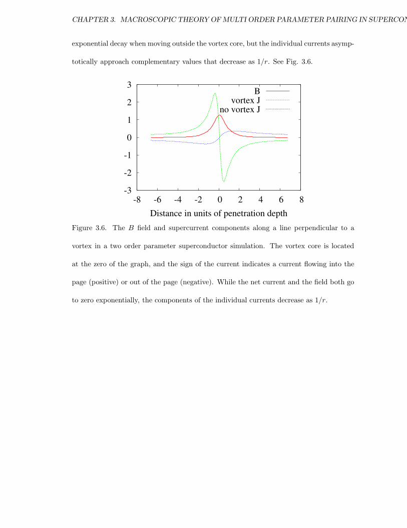
CHAPTER 3. MACROSCOPIC THEORY OF MULTI ORDER PARAMETER PAIRING IN SUPERCONDUCTIITY90
exponential decay when moving outside the vortex core, but the individual currents asymp-
totically approach complementary values that decrease as 1/r. See Fig. 3.6.
-3
-2
-1
0
1
2
3
-8 -6 -4 -2 0 2 4 6 8Distance in units of penetration depth
Bvortex J
no vortex J
Figure 3.6. The B field and supercurrent components along a line perpendicular to a
vortex in a two order parameter superconductor simulation. The vortex core is located
at the zero of the graph, and the sign of the current indicates a current flowing into the
page (positive) or out of the page (negative). While the net current and the field both go
to zero exponentially, the components of the individual currents decrease as 1/r.
CHAPTER 3. MACROSCOPIC THEORY OF MULTI ORDER PARAMETER PAIRING IN SUPERCONDUCTIITY91
This can be understood by considering the two order parameter current operator
when the net current is zero, and assume a gauge where ~A = 0 at the center of the vortex.
If the vortex exists in order parameter 1 then ∇θ1 ∝ 1/r. Since order parameter 2 does
not have a vortex ∇θ2 = 0. The non-zero flux contained in the vortex implies a radially
directed ~A that also goes as 1/r. However no single ~A can individually zero out both the
contributions to the current. The total flux contained in the vortex is
Φ1 =
2z1~πm1
|Ψ1|22z2
1
m1|Ψ1|2 +
2z22
m2|Ψ2|2
. (3.34)
Due to the 1/r current density, the energy associated with a unpaired vortex grows log-
arithmically with the size of the system. If the system contains a vortex pair that have
been separated due to thermal fluctuations or other mechanism, the energy will grow log-
arithmically with the separation. This will produce a long range attractive force that goes
as 1/r. There will also be an angle dependence that goes as
~F ∝ −B1 · B2 (3.35)
where Bx is a convenient way to indicate the direction the vortex, but it is not intended
to indicate that this force is from the magnetic energy..
3.9 The bi-quadratic term
A rationalization for the bi-quadratic term, γνµ|Ψν |2|Ψµ|2, is a competition be-
tween the two condensates for carriers. One example could be two FFLO phases with
different pair momentum.

CHAPTER 3. MACROSCOPIC THEORY OF MULTI ORDER PARAMETER PAIRING IN SUPERCONDUCTIITY92
It is possible for the bi-quadratic term to be large enough that it prevents the
coexistence of both phases. In this case the superconductor will phase separate. If one of
the condensates is energetically favorable, it will completely dominate. Since the dominant
order parameter would be suppressed in the center of a vortex, it is possible for the
subordinate phase to exist in the core of a vortex. See Fig. 3.7
Figure 3.7. From a simulation of a long prism shaped superconductor as described in
Fig. 3.2. A vortex in the energetically favorable condensate (red) suppresses the order
parameter enabling the less favored condensate (blue) to exist in the vortex core.

CHAPTER 3. MACROSCOPIC THEORY OF MULTI ORDER PARAMETER PAIRING IN SUPERCONDUCTIITY93
In the case where multiple order parameters coexist, the bi-quadratic term will
provide either a local attractive or repulsive force between vortices in different condensates
depending on the sign of the term.
3.10 The Josephson term
A possible rationalization for the bi-linear Josephson term, σνµΨνΨ∗µ, could be
hopping between condensates. The two gap superconductors such as MgB2 may be pos-
sible candidates. The complex phase of the coefficient σνµ will only effect the preferred
relative phase of the order parameters, so I will assume that σνµ ≤ 0 and real, such that
matching phases minimize the energy.
The Josephson term causes the symmetry for all bi-linear coupled condensates to
be broken with the formation of the first condensate. Also, the Josephson term produces
a much stronger coupling between condensates than either the ~A field or the bi-quadratic
term. For this reason, it is difficult to determine if a superconductor actually has two
condensates, or one condensate with two gaps. For clarity, I will define a two order
parameter superconductor to be one where both condensates can exist when the Josephson
term is frustrated.
The strength of the coupling of the Josephson term can be illustrated by con-
sidering the case were each order parameter contains a single vortex which are separated
by many coherence lengths. See Fig. 3.8. All Josephson energy iso-curves pass through
the center of the vortices. The shape of each iso-curve is fixed, but the overall scale grows

CHAPTER 3. MACROSCOPIC THEORY OF MULTI ORDER PARAMETER PAIRING IN SUPERCONDUCTIITY94
linearly with the separation, r, of the vortices. The energy will increase as r2 since it is
proportional to the area, and will quickly exceed the short range bi-quadratic energies and
long range logarithmic ~A field coupling.
Figure 3.8. The arrows represent the phase of two condensates, each with a single vortex.
The vortices are off set from each other to illustrate the effect of relative order parameter
phases. The energy associated with the Josephson coupling is proportional to minus the
cosine of the difference in the phases. The line between the vortices shows the maximum
phase difference and therefore the highest energy density. The curve where the energy
contribution is zero forms a circle with the vortex centers on the perimeter.
CHAPTER 3. MACROSCOPIC THEORY OF MULTI ORDER PARAMETER PAIRING IN SUPERCONDUCTIITY95
The preceding argument assumed no charge transfer between condensates. This
would certainly be true for the theoretical electron and proton condensates of hydrogen.
If it is assumed that some charge transfer does occur, such as a Josephson hopping current
Jhopping ∝ |Ψ1||Ψ2|sin(θ2 − θ1) (3.36)
the situation changes considerably. The flow of current between condensates will provide
a mechanism by which the phase frustration can be reduced. Figure 3.9 is a three di-
mensional simulation of a two order parameter block of superconductor. The phase of
both condensates is roughly equal throughout the simulation except in the space between
the vortices indicated by the thin red “J-wall”. Following a path around the blue vortex
but not the gold one, one expects the phase of the blue condensate to go through 2π,
while the gold condensate will have a phase change of zero. When the phase integration is
performed, one finds that both condensates collect a phase change of approximately π in
the region that excludes area near the J-wall. In the region between the vortices, the blue
condensate will pick up an additional phase of π while the gold condensate will pick up an
canceling phase of −π. The energy associated with the Josephson term is now confined to
the J-wall (whose area is proportional to r). The energy associated with the separation
of the vortices will be proportional to r.
Well outside the vortex cores and the J-wall, the net current is zero. Since the
phases of the condensates are equal, the individual components of the current must also
be zero. Well outside the vortex cores but within the J-wall, the net current is still zero,
but the components will have equal and opposite currents.

CHAPTER 3. MACROSCOPIC THEORY OF MULTI ORDER PARAMETER PAIRING IN SUPERCONDUCTIITY96
Figure 3.9. This figure is from a 3 dimensional simulation of a two order parameter
superconductor with a Josephson coupling term. The iso-surface of the order parameters
in gold and blue show a single vortex each. The thin red wall of phase frustration or “J-
wall” is an iso-surface of the Josephson energy corresponding to a value of zero. Without
inter-condensate currents, this iso-surface would have a circular cross section. See Fig.
3.8.

CHAPTER 3. MACROSCOPIC THEORY OF MULTI ORDER PARAMETER PAIRING IN SUPERCONDUCTIITY97
3.11 J-wall excitations
In the previous section, the J-wall was bordered by either a vortex or the edge
of the superconductor. It is also topologically possible for J-wall excitations to exist as
closed surfaces. For example consider a spherically symmetric case where both condensates
order parameters are real and positive at the origin. At some distance which is several
coherence lengths from the origin, one order parameter goes through a phase change of π
while the other goes through a phase change of −π. Outside the region where the phases
are changing, each order parameter has a phase that is real and negative. This J-wall
forms a sphere with energy proportional to its surface area.
The surface of a J-wall is directed since each condensate flows in definite direction.
For convention, assume that the positive direction for a J-wall is the direction that adds
π to θ1. Two oppositely oriented J-walls will experience a short range attraction and will
annihilate each other. Two J-walls oriented in same direction will experience a short range
repulsion.
Since the J-walls do not couple to the magnetic field, they will be difficult to
induce or detect in any material in which multiple condensates are suspected. One pos-
sibility for inducing J-walls would be to preferentially drive a tunneling current into only
one condensate causing a phase slip between the condensates. It is not clear how to detect
when this occurs however.
It may be possible to detect a phase transition where thermally induced J-walls
freeze out. The lowest J-Wall excitations would have a finite energy since the length scale
CHAPTER 3. MACROSCOPIC THEORY OF MULTI ORDER PARAMETER PAIRING IN SUPERCONDUCTIITY98
of the smallest J-wall excitation must be on the order of the coherence length. Below this
length scale, the order parameters could not make a full rotation of |π|. Excitations on this
scale are not disallowed, but they would tend to be spherical and have an energy that is
proportional to their volume. Above this minimum energy, the number of configurations
(states) per energy level becomes large since it is not longer limited to being spherical
and the energy is proportional to the area. If the low energy excitations are ignored, the
sudden rise in density of states at a finite energy and domain wall like behavior gives rise
to the Potts model like behavior[80][81].
3.12 Not any knots
There has been interest in knots in multi component Bose Einstein models [82]
[83]. The structures considered in these papers were beyond what my numerical model
could simulate. Small vortex knot components were considered and found to be unstable.
See Fig. 3.10 for a couple of attempts. The knot components were intended to use the
repulsion of vortices to overcome the tendency of a vortex to minimize its length. Vortex
tension was found to be stronger than repulsion causing the vortices to pass through one
another.

CHAPTER 3. MACROSCOPIC THEORY OF MULTI ORDER PARAMETER PAIRING IN SUPERCONDUCTIITY99
Twist Cross
Figure 3.10. Two attempts at building vortex knots. In all variations of the “twist”
attempted, with naturally repelling vortices, the vortices ultimately passed through each
other rather than untwisting. With careful positioning, two normally repelling vortices
can be attached in a “cross” arrangement to form an unstable bond. When disturbed,
the point of intersection will move toward the nearest normal boundary and exit the
superconductor.

CHAPTER 3. MACROSCOPIC THEORY OF MULTI ORDER PARAMETER PAIRING IN SUPERCONDUCTIITY100
3.13 Conclusion
I have developed a fast and efficient numerical method for solving the Ginsburg-
Landau model of superconductivity in 2 and 3 dimensions. This method included extensive
visualization and interaction. The model was used to study the interaction of supercon-
ductivity and magnetic fields with particular emphasis on vortex dynamics.
The model was then extended to include multiple condensate order parameters.
This extended model was used to study potentially stable vortex knots with negative re-
sults. An interesting topological excitation was found associated when a bi-linear Joseph-
son coupling term was included in the simulations.

Chapter 4
Classical Spin Systems
101

CHAPTER 4. CLASSICAL SPIN SYSTEMS 102
4.1 Introduction
The properties of both 2D square Ising and Edwards-Anderson spin glass model
have been studied for many years. The Ising model
H = −∑
<i,j>
SiSj (4.1)
with nearest neighbor interactions was solved by Onsanger using transfer matrix methods.
The 3D model is considered to fall into a class of NP complete problems that are unsolvable
[84], and therefore must be attacked with approximate methods.
The nearest neighbor Edwards-Anderson spin glass energy is
H = −∑
<i,j>
JijSiSj (4.2)
where Jij has some random distribution. The two most common distributions are the
bimodal where J = ±1 and the continuous where J has a distribution that normally is
taken to be Gaussian. These models are also unsolved, but a number of methods have
been developed to study their properties. The ground state of large systems [85] can be
calculated quickly and efficiently making T = 0 investigations possible. Sampling methods
such as Monti Carlo run into problems due to the slow dynamics below Tc. However
improved methods such as tempering [86] have been developed which have enabled progress
in 3D investigations [87].
The numerical transfer matrix methods have also been applied to spin glasses
[88][89][90], but due to the exponential growth in the memory and simulation time with
the width of the system, the size of systems must be limited. As long as Moore’s law

CHAPTER 4. CLASSICAL SPIN SYSTEMS 103
continues to hold however, one can expect to add a site to the width of the calculation
every couple of years. I have developed efficient algorithms for solving finite size spin glass
systems using the transfer matrix method and applied them to Ising an Edwards-Anderson
spin systems.
4.2 Transfer matrix applied to spin systems.
Calculating the partition function,
Z =∑
C
e−ECβ (4.3)
where C goes over all configurations, is in principle straight forward. In practice, it is
difficult due to the the number of configurations. Each spin in the system doubles the
number of terms in the sum giving a total of 2M configurations M is the number of spins.
The transfer matrix method as applied to spin systems is a method for reducing
the number of additions that need to be performed to calculate Z. There is quite a bit
of flexibility in defining a transfer matrix, therefore I will describe one implementation
while pointing out where degrees of freedom exist. Referring to figure 4.1, the transfer
matrix T (A,B) is defined such that it includes all the terms of the partition function sum
for all intra-yellow bonds and the bonds between the yellow spins and the spin cuts. The
contribution from the bonds between the spins in each cut must be accounted for, but
care must be taken not to count them twice. I choose to include the bonds in cut A in
T (A,B), but not the bonds in cut B. The bonds in cut B will be accounted for in another
transfer matrix.

CHAPTER 4. CLASSICAL SPIN SYSTEMS 104
Figure 4.1. The colored squares represent spin sites. The connections between the sites
represent bonds. The spins in the cuts must completely separate the spins on either side
of the cut such that no direct bond connects sites on one side of the cut to the other side of
the cut. Since this system has only nearest neighbor bonds, the cut need only be one spin
wide. If however the bonds to next nearest neighbor were also included, the cut would
need to be two spins wide.
In this example each cut contains four spins for a total of 16 states. The rows of
T (A,B) are indexed by the states of cut A while the columns are indexed by the states of
cut B. (The exponential cost has not been completely eliminated but only reduced. This
is the major weakness of the transfer matrix method and places practical limits on the
cut size.) An entry of the transfer matrix is defined as
Tij(A,B) =∑
C′
e−EC′β (4.4)
where the energy only includes the bonds listed above, the sites in cut A are in state i, the
sites in cut B are in state j, and the index C ′ goes over all configurations of the “yellow”
sites between the two cuts.

CHAPTER 4. CLASSICAL SPIN SYSTEMS 105
Now assume that I have the matrix T (A,B) and the matrix T (B,C), where C
is another cut line further to the right, and I want the matrix T (A,C). Following the
standard derivation, first consider the matrix
R(j) = T (A,B)|j >< j|T (B,C) (4.5)
where j selects a single state of B. An entry of B is
Rik(j) =∑
C′
e−EC′β∑
C′′
e−EC′′β =∑
C′
∑
C′′
e(−EC′−EC′′ )β (4.6)
where the index C ′′ goes over all configuration of sites between cut B and cut C. The
nested sum now goes over all configurations of spins between A and C with the spins of
cut B in state j. If I then sum over all all states of B, I find I have T (A,C) by definition.
Performing the sum gives
T (A,C) =∑
j
T (A,B)|j >< j|T (B,C)
= T (A,B)∑
j
|j >< j|T (B,C)
= T (A,B)T (B,C) (4.7)
which is just simple matrix multiplication.
If the system is open on the ends, the last transfer matrix will need to include
the energy for the bonds in the final cut. The partition function is found by summing
over all the combined configurations of the starting cut and the ending cut. In term of
the final matrix, this becomes
Z =∑
i
∑
j
Tij(Start, End) =< Ω|T (Start, End)|Ω > (4.8)

CHAPTER 4. CLASSICAL SPIN SYSTEMS 106
where |Ω > is a vector of all 1s.
For periodic boundary conditions, the starting and ending cut are the same
and no special handling of the last matrix is necessary. After the final transfer matrix
multiplication, only the diagonal terms contribute. The partition function in this case is
just given by
Z =∑
i
Tii(Start, Start) = Tr[T (Start, Start)] (4.9)
It is customary to define the incremental transfer matrix to have a step of one
row with no intervening sites. This is cheaper since calculating all the intervening “yellow”
spins becomes unnecessary. The original cost went as 2M . The cost of the transfer matrix
goes as
2N∗3 × L (4.10)
Where N width of the cut and L is the length of the system.
4.3 One spin at a time
One degree of freedom in defining the transfer matrix (not mentioned in the
previous section) is how the cuts are defined. There is no requirement that the cuts go
straight across or that they are non-overlapping. Referring to figure 4.2, the transfer
matrix is defined such that only one site is added and one site is removed. The transfer
matrix still needs to include all configurations for each cut, but now the cuts are not
longer independent. Any entry in the new T (A,B) that conflicts with the shared sites

CHAPTER 4. CLASSICAL SPIN SYSTEMS 107
must be zero. (I have not been able to find a reference of this method of transfer matrix
calculation, bit it seems likely to have been done before. The performance matches 2N
best case perfromance mentioned by A. P. Young)
Figure 4.2. The colored squares represent spin sites. The connections between the sites
represent bonds. The spin cuts in this case overlap. The red site is unique to cut A, the
blue site is unique to cut B, and the pink sites are shared. Both sites meet the bond cut
requirement between the green and purple sites.

CHAPTER 4. CLASSICAL SPIN SYSTEMS 108
The new matrix is defined as: (1)the bonds used to calculate T (A,B) are only
the ones that connect to the “Red” site. (2)The configurations of the cut are indexed as
a binary number where and up spin is a one and a down spin is a zero. (3)The most most
significant bit of cut A is the “Red” site.(4)The least significant bit of cut B is the “Blue”
site. Assuming no external field, the new one step transfer matrix is
T (A,B) =
a b 0 0 0 0 0 0
0 0 c d 0 0 0 0
0 0 0 0 e f 0 0
0 0 0 0 0 0 g h
h g 0 0 0 0 0 0
0 0 f e 0 0 0 0
0 0 0 0 d c 0 0
0 0 0 0 0 0 b a
(4.11)
where a − h are Boltzmann terms based on the bond energies. Because of the bonds
chosen and the ordering of states, there is a symmetry associated with inversion of all
spins that becomes obvious. This symmetry will cause the eigen vectors to be either odd
or even. Since all non-zero entries must be positive, one would expect an even eigen vector
to always have the largest eigen value. Long range order however requires that the largest
odd and even eigen vector become degenerate. This paradox is resolved by noting that
long range order does not occur in systems with finite width.
This overlapping of spin cuts turns out to be a big win in the cost of calculations.

CHAPTER 4. CLASSICAL SPIN SYSTEMS 109
The cost of using this sparse transfer matrix to calculate Z goes as
2N∗2 × L×N (4.12)
Note the exponent associated with the matrix multiplications has been decreased by N
with only an additional scaling term of N. This may not seem like a lot, but this can be
a factor of several thousand when N starts getting big.
So far, I have only considered calculating the partition function completely.
When the system being considered lacks long range order, as one dimensional systems
do, it may be acceptable to calculate only a few columns of the final transfer matrix [90].
This is equivalent to limiting the number of starting and stopping configurations. When
this is done, the cost of the partition function calculation goes as
2N × L×N ×W (4.13)
where W is the number of rows of the transfer matrix calculated.
As noted above, the eigen vectors of the one step transfer matrix can separated
into even and odd sets. The transfer matrix does not mix the two sets. This creates the
possibility of calculating the even an odd parts of the transfer matrix product separately.
The odd transfer matrix becomes
Todd(A,B) =
a b 0 0
0 0 c d
0 0 −f −e
−h −g 0 0
(4.14)

CHAPTER 4. CLASSICAL SPIN SYSTEMS 110
where Teven(A,B) would differ only in that all entries would be positive. This optimization
cuts the cost of partition function calculation in half. This optimization does not work
with any applied field that breaks inversion symmetry, therefore I have not used this
optimization in calculations.
4.4 Finite T computations
In the algorithm that performs the calculation, none of the transfer matrices are
ever actually stored. The heart of the algorithm is a subroutine that takes as input a vector
of size 2N “real” floating point values, the bond strength and Zeeman splitting energy. It
performs the matrix multiplication and returns the result in another 2N size vector. To
calculate a column of the transfer matrix, the algorithm starts with a unit vector that
represents a single configuration of the initial cut, then the subroutine is called once for
each spin with the appropriate bonds. This can be written as
|Tj >=∏
i
T (i)|j > (4.15)
where |Tj > is a column vector representing column j of the transfer matrix product. If
the full calculation is desired, this is repeated for each configuration in the initial cut.
The number of spins in the spin cut is limited by computation time and computer
memory. For example, a cut of 26 spins consumes one giga-byte of memory and takes about
1 second to perform a matrix multiplication on a relative modern computer (2 giga-Hertz
and 2 giga-byte of DRAM). For each spin removed from the cut, the memory and time
required to perform a single vector update is cut by half.
CHAPTER 4. CLASSICAL SPIN SYSTEMS 111
The temperature range to which this method can be applied is limited by the ac-
curacy of the numerical representation of real numbers. The magnitude of the entries in the
one step transfer matrix for the ±1 model range from ∼ exp(−1/T ) to ∼ exp(1/T ) which
puts the absolute range of the terms in the partition function sum to be ∼ exp(±M/T ).
As T gets small, the terms closer to exp(+M/T ) will dominate.
The lower bound in T is determined by the observable that is being calculated.
For example, the calculation of entropy
S = ln(Z) +T
Z
dZ
dT(4.16)
involves a single derivative. Finite difference is the obvious choice for calculating deriva-
tives, unfortunately this involves subtracting two large numbers to produce a small number
greatly reduces the usable number of bits of precision. Specific heat,
Cv = 2T
Z2
dZ
dT+T 2
Z
d2Z
dT 2(4.17)
requires a second derivative which requires performing the subtraction twice. The specific
heat calculation on small systems ,N = 10 and L = 100, seem to be valid down to T ≈ .5
in units of J . Fortunately this is below the transition temperatures for both ordered and
glassy spin systems.
4.5 Partition function polynomial and T = 0 calculations
Another way to view the partition function is to think of it as a polynomial
Z =∑
i
Aie−Eiβ (4.18)
CHAPTER 4. CLASSICAL SPIN SYSTEMS 112
where Ei is the ith energy above the ground state. Ai is the degeneracy of ith energy
level. In order to put the degeneracy on the same footing as Eβ, assume ai = ln(Ai). The
partition function becomes
Z =∑
i
e(ai−Eiβ). (4.19)
For systems such as the ferromagnetic, antiferromagnetic or ±1 models, the number of
terms will be on the order of the number of spins in the system. The coefficients ai is the
log of the density of states. There have been some attempts to calculate this polynomial
for small systems using non-transfer matrix methods [91][92] and an interesting truncated
transfer matrix method by Morgenstern and Binder[89]
Calculating the polynomial is conceptually simple if one assumes a polynomial
data type that includes the operations of poly-add and poly-scale. Poly-add adds two
polynomials to produce a new polynomial. Poly scale multiplies a polynomial by e(a−Eβ).
It is also useful to include a clipping option to only keep a fixed number of the lowest
energy terms. This new data type replaces the real data type in the algorithm described
above. This method is not without its cost however. It takes on the order of six minutes
to calculate the full polynomial for a 10 by 10 spin system with this new method where it
takes only 3.5 seconds to perform a real calculation for a single T. On the other hand it
only takes 8 seconds to calculate the ground state term.
There are several advantages of this method over the “real” method. The most
obvious being that once the complete polynomial has been calculated, the partition func-
tion is known for all temperatures. The T = 0 entropy is given by the log of the degeneracy

CHAPTER 4. CLASSICAL SPIN SYSTEMS 113
of the ground state and approaches the approaches the published bulk value[101],0.078.
The fact the Z becomes very large can easily be dealt with by factoring out the largest
term
Z = e(ax−Exβ)∑
i
e(ai−Eiβ−(ax−Exβ)). (4.20)
where the xth term is the largest. Each term in the sum is now less than or equal to one,
and the large exponential factored out will cancel when an observable is calculated.
4.6 2D Ising phase transition
The 2D Ising phase ferromagnetic phase transition has been solved and is well
understood, but it still can be enlightening to consider this case however.
As mentioned before, the largest contribution to the partition function comes
from the term with the largest value of (ax −Exβ). For large systems and finite T , there
will be many samples around the largest term that also contribute. In this case, it is
reasonable to consider the case where a is a continuous function of E. The partition
function then becomes
Z =∑
i
e(ai−Eiβ) ≈ 1
4
∫
dEe(a(E)−Eβ) (4.21)
where the 1/4 scaling is required because the discrete energy levels occur in steps of four
(in units of J). The function a(E) can be thought of as a log of the density of states.
The value of E where (a(E) − Eβ) is maximum for a given temperature is found by the
CHAPTER 4. CLASSICAL SPIN SYSTEMS 114
standard method
d
dE(a(E) −Eβ) =
da(E)
dE− β = 0. (4.22)
Solving for the inverse temperature gives
β =da(E)
dE(4.23)
where T = 1/β. As long as the second derivative of a(E) is less than zero, to first
approximation the energies around the maximum will contribute to observable calculations
with a Gaussian weighting.
Figure 4.3 is a graph of a(E) for a 12 by 70 site ferromagnetic Ising system. For
a system with a smooth, convex a(E), the specific heat can be approximated by
Cv ≈−
(
da(E)dE
)2
d2a(E)dE2
≈ −(
T 2d2a(E)
dE2
)−1
. (4.24)
Near the center of the graph, one can see how the curvature approaches zero. This will
cause the specific heat to diverge indicating a second order phase transition.
The specific heat calculated using equation 4.17 for a range of system configura-
tions is shown in figure 4.4.
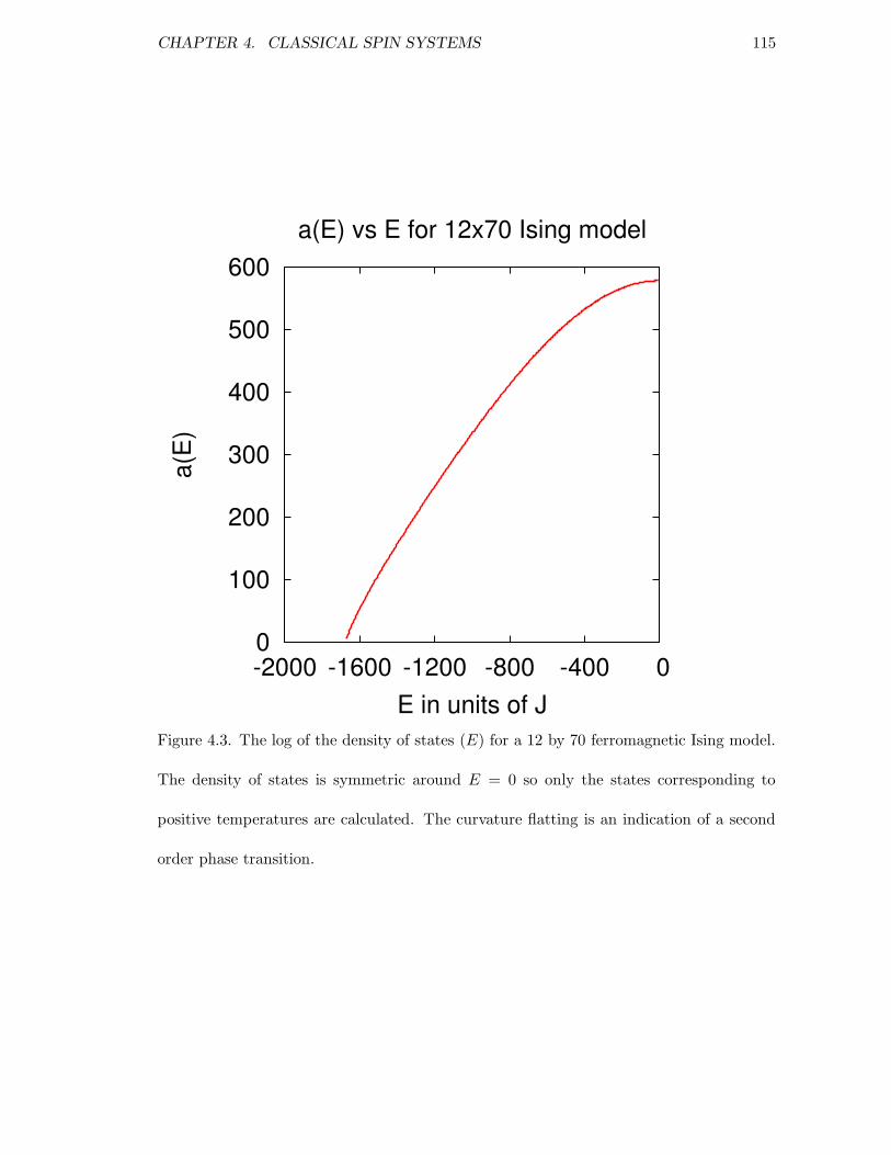
CHAPTER 4. CLASSICAL SPIN SYSTEMS 115
0
100
200
300
400
500
600
-2000 -1600 -1200 -800 -400 0
a(E)
E in units of J
a(E) vs E for 12x70 Ising model
Figure 4.3. The log of the density of states (E) for a 12 by 70 ferromagnetic Ising model.
The density of states is symmetric around E = 0 so only the states corresponding to
positive temperatures are calculated. The curvature flatting is an indication of a second
order phase transition.

CHAPTER 4. CLASSICAL SPIN SYSTEMS 116
0 0.2 0.4 0.6 0.8
1 1.2 1.4 1.6 1.8
0 1 2 3 4
Cv
T in units of J
FM Ising Specific Heat
12x7010x848x1056x1404x210
18x50020x500
Figure 4.4. The specific heat for a range of system configurations showing approaching
divergence as the geometry of the system goes from one dimensional to two dimensional.
The systems represented by lines were produced from full partition function polynomial
calculations. The systems represented by points were produced from real calculations of
one row from the transfer matrix.

CHAPTER 4. CLASSICAL SPIN SYSTEMS 117
4.7 Spin Glass
Glassy systems in general are characterized by taking a long time to reach ther-
modynamic equilibrium, and in most cases this time becomes infinite. This is is generally
attributed to the presence of energy barriers between local energy minimum which prevent
the thermal excited exploration of configuration space.
4.8 Trapping local energy minimum
An example without quenched disorder, consider a magnetic that is modeled
by the classical, rectangular, two dimensional, ferromagnetic Ising model with nearest
neighbor interactions. The Hamiltonian is
H = −∑
<i,j>
JijSiSj (4.25)
where the sum goes over all nearest neighbors, Jij = 1, and Sα = ±1. The ground state
is known to be all Sα = 1 or all Sα = −1. If this system is suddenly quenched from a
temperature well above Tc to a temperature well below Tc , one expects to find that the
magnetization is defined by
m =1
M
∑
i
Si =< S > (4.26)
where M is the total number of spins, to approach ±1. If one assumes one spin at a
time transitions and the absence of system spanning domain walls, it is possible go from
a disordered state to one of the ground states making only transitions which reduce the
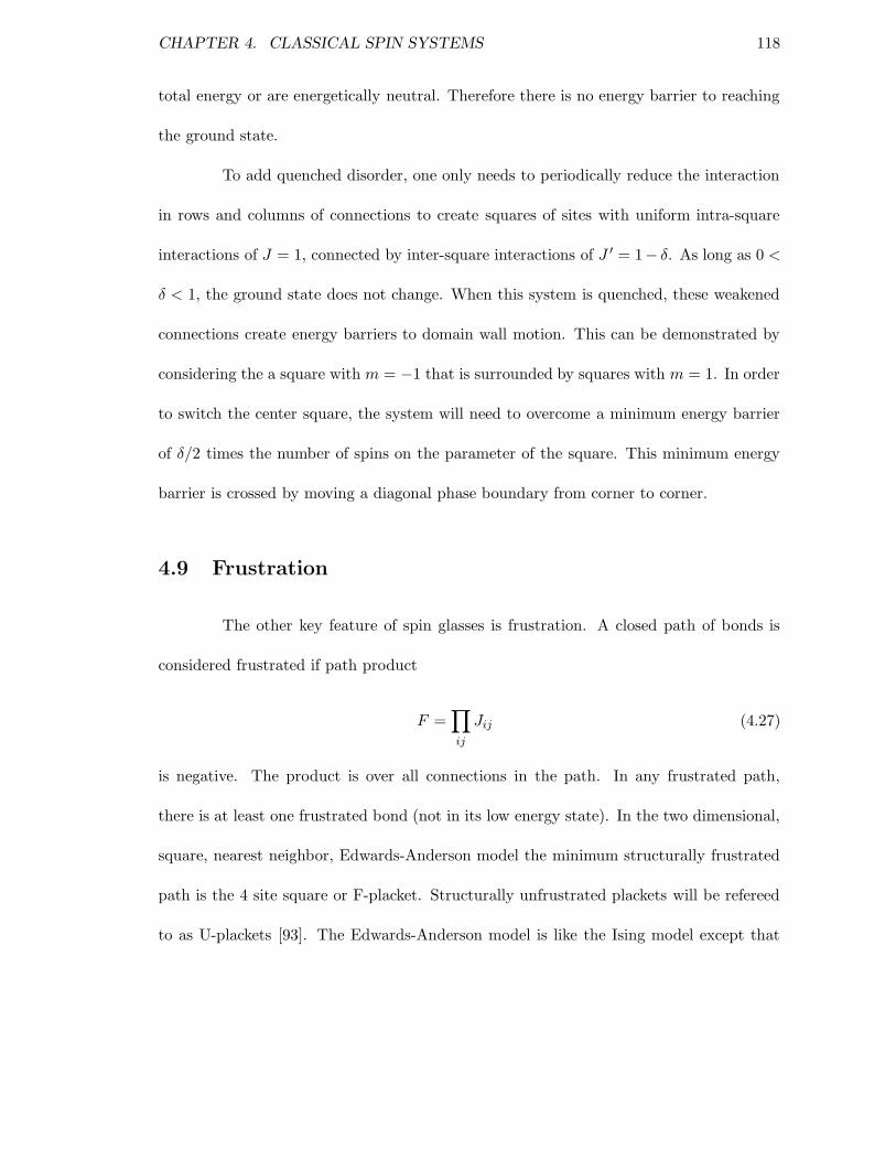
CHAPTER 4. CLASSICAL SPIN SYSTEMS 118
total energy or are energetically neutral. Therefore there is no energy barrier to reaching
the ground state.
To add quenched disorder, one only needs to periodically reduce the interaction
in rows and columns of connections to create squares of sites with uniform intra-square
interactions of J = 1, connected by inter-square interactions of J ′ = 1− δ. As long as 0 <
δ < 1, the ground state does not change. When this system is quenched, these weakened
connections create energy barriers to domain wall motion. This can be demonstrated by
considering the a square with m = −1 that is surrounded by squares with m = 1. In order
to switch the center square, the system will need to overcome a minimum energy barrier
of δ/2 times the number of spins on the parameter of the square. This minimum energy
barrier is crossed by moving a diagonal phase boundary from corner to corner.
4.9 Frustration
The other key feature of spin glasses is frustration. A closed path of bonds is
considered frustrated if path product
F =∏
ij
Jij (4.27)
is negative. The product is over all connections in the path. In any frustrated path,
there is at least one frustrated bond (not in its low energy state). In the two dimensional,
square, nearest neighbor, Edwards-Anderson model the minimum structurally frustrated
path is the 4 site square or F-placket. Structurally unfrustrated plackets will be refereed
to as U-plackets [93]. The Edwards-Anderson model is like the Ising model except that

CHAPTER 4. CLASSICAL SPIN SYSTEMS 119
Jij = ±1 with some random distribution.
The F-placket has some properties similar to the winding number associated with
vortices in type II superconductors. A positive sign of path product, F , indicates that
an even number of F-plackets are enclosed while a negative sign indicates that an odd
number are enclosed. This can easily be demonstrated by starting with a arbitrary path
where F has a definite sign. When the path is increased to enclose another placket, one to
three edges are removed and one to three edges are added such that the total is 4 edges.
If the sign of F changes, then the sign of the path product for the edges removed must be
different from the sign of the path product of edges added. Therefore the path product
for the added placket must be negative indicating it is an F-placket. To complete the
argument, start with a single placket and add packets to for any arbitrary path.
This placket parity forces F-plackets to form pairs connected by a path of doubly
frustrated U-plackets. While U-plackets are not structurally frustrated, they still can have
an even number of frustrated bonds. Figure 4.5 illustrates the ground state of a system
containing four F-plackets. The energy of the system is minimum when the number of
doubly frustrated U-plackets needed to connect all F-plackets in the system is minimized.
This pair formation is also responsible for the presence of quenched disorder in
Edwards-Anderson models. If the pairing had instead been horizontal in figure 4.5 such
that the upper two F-plackets were paired and the lower two were paired, there would be
a energy barrier that would have to be crossed to transition to the ground state.

CHAPTER 4. CLASSICAL SPIN SYSTEMS 120
Figure 4.5. A graphical representation of one of the ground states of a spin system con-
taining four structurally frustrated F-plackets. The red squares represent F-plackets. The
blue squares represent structurally unfrustrated U-plackets. The black lines are unfrus-
trated bonds. The yellow bars are frustrated bonds. In any configuration of spins, there
will always be a path that starts in a F-placket crosses only frustrated bonds, and ends
in an F-placket (or in the case of open boundaries, exits that system). The total taxi cab
length of these paths will be minimized in the ground state.

CHAPTER 4. CLASSICAL SPIN SYSTEMS 121
4.10 2D ±1 glass simulations
The spin glass transition is not an equilibrium transition like the Ising ferromag-
netic transition. It is instead a transition from a paramagnetic state to a quenched state
where the system gets trapped in a local energy minimum. Below the transition temper-
ature TG, the system dynamics become very slow. The dynamics generally considered to
become logarithmic in time reflecting a 1/f distribution of energy barriers. The number of
energy minima grows exponentially with the size of the system making sampling methods
such as Monti Carlo difficult. Multi-temperature methods have shown some success [].
The transfer matrix method avoids the local trapping problems by considering
all possible configurations. So by design, it captures the equilibrium statistics that would
only be accessible as time approaches infinity. The density of states function for a ±1
system does not show any flattening that would indicate a phase transition. See figure
4.6. The The function a(E) is much closer to an ellipse. As expected, the equilibrium
specific heat does not show a divergent behavior. See figure 4.7
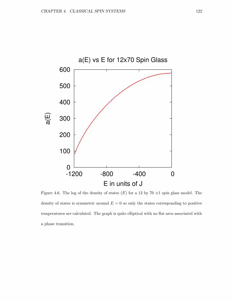
CHAPTER 4. CLASSICAL SPIN SYSTEMS 122
0
100
200
300
400
500
600
-1200 -800 -400 0
a(E)
E in units of J
a(E) vs E for 12x70 Spin Glass
Figure 4.6. The log of the density of states (E) for a 12 by 70 ±1 spin glass model. The
density of states is symmetric around E = 0 so only the states corresponding to positive
temperatures are calculated. The graph is quite elliptical with no flat area associated with
a phase transition.

CHAPTER 4. CLASSICAL SPIN SYSTEMS 123
0 0.05
0.1 0.15
0.2 0.25
0.3 0.35
0.4 0.45
0 1 2 3 4
Cv
T in units of J
Spin Glass Specific Heat
12x7010x848x1056x1404x210
18x50020x500
Figure 4.7. The specific heat for a range of system configurations shows no divergence
behavior. The variations between simulations seems to be due more to the the particular
disorder in the bonds than the system size. The systems represented by lines were produced
from full partition function polynomial calculations. The systems represented by points
were produced from real calculations of one row from the transfer matrix.
CHAPTER 4. CLASSICAL SPIN SYSTEMS 124
4.11 2D continuous bond distribution glass simulation
When the bonds in a spin glass have a continuous distribution, each state has a
degeneracy of 2. This causes the partition function polynomial to have 2M−1 unique terms
making a complete calculation intractable. One possibility to get around this limitation
is to use energy binning to force degeneracy for nearly degenerate states. This has shown
some promise, but I have yet to quantify the error.
The lack of degeneracy creates the possibility of calculating exact ground and
excited states. By fixing one spin in the system, each term of the polynomial is associated
with a unique configuration which can be tracked. The ground state has been verified
using the Spin Server provided online by the Institut fr Informatik. The ground state
and first three excited states for a 10 by 10 spin system with Gaussian bond distribution
is shown below. In the ground state, up spins are indicated by “+” and down spins by
a “−”. In the excited states, an “=” sign indicates a ground state matching spin and
an “∗” indicates a flipped spin. The large number of flipped spins in the third excited
state illustrates how a local minimum can be a large distance (as measured in number of
differing spins) from the ground state.

CHAPTER 4. CLASSICAL SPIN SYSTEMS 125
Ground E = 0.048 E = 0.124 E = 0.163
− + −− + −−−−+ ========== ========== == ∗ ∗ ∗ ∗ ∗∗ ==
−− + + −−−−−+ ========== ========== == ∗ ∗ ∗ ∗ ∗ ∗ ∗ =
− + + + −− + −−+ == ∗∗ ====== ========== ==== ∗ ∗ ∗ ∗ ∗ =
+ + + + + + + − ++ ========== ========== == ∗ ∗ ∗ ∗ ∗ ∗ ∗∗
+ + + −−−−− ++ ========== ========== == ∗ ∗ ∗ ∗ ∗ ∗ ∗∗
+ −− + −− + + −+ ========== == ∗∗ ====== ==== ∗ ∗ ∗ ∗ ∗ =
− + −−− + −−−+ ========== == ∗∗ ====== ==== ∗∗ ====
+ + − + − + + − ++ ========== ========== ==========
−−− + − + + + ++ ========== ========== ==========
+ + − + −−− + −− ========== ========== ===== ∗ ∗ ∗ ==
Another way to analyze is to analyze the behavior is to consider the spin-spin
correlation verses distance at finite temperatures. As the transfer matrix product is created
by incorporating more spins through matrix multiplication
Trunning =∏
s=0−i
Ts (4.28)
the current product matrix quickly assumes a very singular form
Trunning = λOdd|OddR >< OddL|λEven|EvenR >< EvenL| (4.29)
with all other eigenvalues becoming tiny. At T = 0 it is expected that λEven ∼ λOdd as
the number of spins grows large indicating long range order. At T > TSG it is expected that

CHAPTER 4. CLASSICAL SPIN SYSTEMS 126
λEven >> λOdd indicating no long range order. Figure 4.8 illustrates how the eigenvalues
change with distance along a long 18 spin wide strip. The quantity graphed,
Γ = log
(
λOddsqrtλ2
Odd + λ2Even
)
(4.30)
indicates how correlated a states at the start of the strip are to the states at the end
of the strip. At the highest temperature, T = 0.35, Γ shows a noisy but steady decline
representing an exponential loss of correlation. Between T = 0.25 and T = 0.15 , flat
portions start appearing representing highly correlated regions. These correlated regions
are responsible for the energy barriers that cause the slow spin glass dynamics below TSG.
At T = 0.05, the graph is mostly flat with a few noisy steps. These steps are caused by
low energy excitations that span the width of the strip. At any finite temperature, these
excitations will cause the loss of long range order. Domain spanning excitations will exist
at some density below any finite energy.
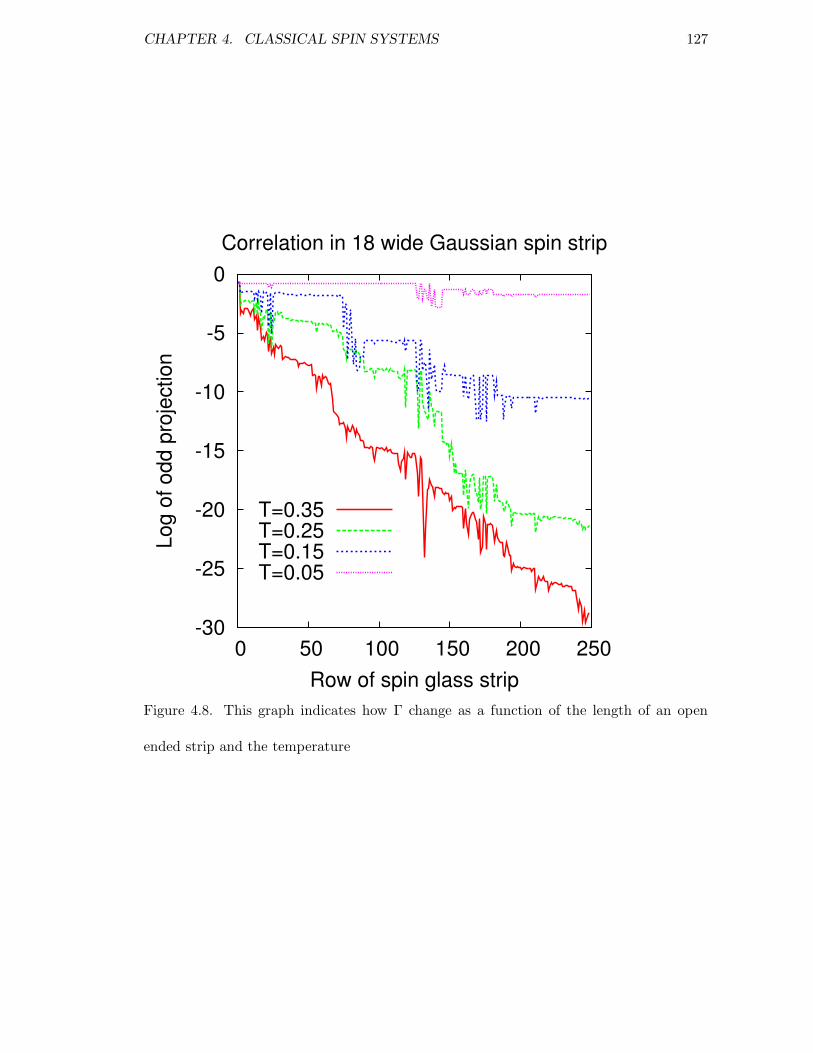
CHAPTER 4. CLASSICAL SPIN SYSTEMS 127
-30
-25
-20
-15
-10
-5
0
0 50 100 150 200 250
Log
of o
dd p
roje
ctio
n
Row of spin glass strip
Correlation in 18 wide Gaussian spin strip
T=0.35T=0.25T=0.15T=0.05
Figure 4.8. This graph indicates how Γ change as a function of the length of an open
ended strip and the temperature

CHAPTER 4. CLASSICAL SPIN SYSTEMS 128
4.12 Conclusion
The exponential advancement of computers enables the revisiting of problems
from time to time. I have developed transfer matrix algorithms for the calculation of the
finite T partition function and the exact polynomial partition function. I have verified
these calculations by compairing them against published results.

Bibliography
[1] V. Ginzburg, Sov. Phys. JETP 4, 153 (1957).
[2] J. Bardeen, L. N. Cooper, and J. R. Schrieffer, Phys. Rev 108, 1175 (1957).
[3] P. Fulde and R. A. Ferrell, Phys. Rev 135, A550 (1964).
[4] A. I. Larkin and Y. N. Ovchinnikov, Sov. Phys. JETP. 20, 762 (1965).
[5] R. Casalbuoni and G. Nardulli, Rev. Mod. Phys. 76, 263 (2004).
[6] L. N. Bulaevskii, Sov. Phys. JETP 38, 634 (1974).
[7] M. S. Nam, J. A. Symington, J. Singleton, S. J. Blundell, A. Ardavan, J. A. Peren-
boom, M. Kurmoo, and P. Day, J. Phys.: Condens. Matter 11, L477 (1999).
[8] S. Manalo and U. Klein, J. Phys.: Condens. Matter 12, L471 (2000).
[9] S. Uji, H. Shinagawa, T. Terashima, T. Yakabe, Y. Teral, M. Tokumoto, A.
Kobayashi, H. Tanaka, and H. Kobayashi, Nature 410, 908 (2001).
[10] L. Balicas, J. S. Brooks, K. Storr, S. Uji, M. Tokumoto, H. Tanaka, H. Kobayashi,
A. Kobayashi, V. Barzykin, and L. P. Gor’kov, Phys. Rev. Lett. 87, 067002 (2001).
129

BIBLIOGRAPHY 130
[11] M. Houzet, A. Buzdin, L. Bulaevskii, and M. Maley, Phys. Rev. Lett. 88, 227001
(2002).
[12] S. Uji, H. Shinagawa, C. Terakura, T. Yakabe, Y. T. M. Tokumoto, A. Kobayashi,
H. Tanaka, and H. Kobayashi, Phys. Rev. B 64, 024531 (2001).
[13] A. Bianchi, R. Movshovich, C. Capan, P. G. Pagliuso, and J. L. Sarrao, Phys. Rev.
Lett. 91, 187004 (2003).
[14] H. Won, K. Maki, S. Haas, N. Oeschler, F. Weickert, and P. Gegenwart, Phys. Rev.
B 69, 180504 (2004).
[15] V. G. Kogan, P. Miranovi/’c, L. Dobrosavljevic-Grujic, W. E. Pickett, and D. K.
Cristen, Phys. Rev. Lett. 79, 741 (1997).
[16] V. G. Kogan, P. Miranovic, L. Dobrosavljevic-Grujic, W. E. Pickett, and D. K.
Cristen, Phys. Rev. Lett. 79, 741 (1997).
[17] S. Graser, T. Dahm, and N. Schopohl, Phys. Rev. B 69, 014511 (2004).
[18] K. G. Sandeman, G. G. Lonzarich, and A. J. Schofield, Phys. Rev. Lett. 90, 167005
(2003).
[19] I. I. Mazin, D. J. Singh, and A. Aguayo, cond-mat/0401563 .
[20] M. Uhlarz, C. Pfleiderer, and S. M. Hayden, Phys. Rev. Lett. 93, 256404 (2004).
[21] N. L. Cooper, Phys. Rev 104, 1189 (1956).

BIBLIOGRAPHY 131
[22] F. London, Superfluids (Wiley, New York, 1950), Vol. 1.
[23] T. V. Duzer and C. Turner, Principles of Superconductive Devices and Cricuits
(Elsevier, New York, 1981).
[24] A. J. Leggett, Rev. Mod. Phys. 47, 331 (1975).
[25] A. P. Mackenzie and Y. Maeno, Rev. Mod. Phys. 75, 657 (2003).
[26] B. J. Powell, J. F. Annett, and B. L. Gyorffy, J. Phys. A 36, 9289 (2003).
[27] H. Shimahara, Phys. Rev. B. 50, 12760 (1994).
[28] K. Koepernik and H. Eschrig, Phys. Rev. B 59, 1743 (1999).
[29] D. J. Singh and I. I. Mazin, Phys. Rev. Lett. 88, 187004 (2002).
[30] E. A. Yelland, S. M. Hayden, S. J. C. Yates, C. Pfleiderer, M. Uhlarz, R. Vollmer,
H. v. Lhneysen, N. R. Bernhoeft, R. P. Smith, S. S. Saxena, and N. Kimura, Phys.
Rev. B. 72, 214523 (2005).
[31] H. Saji, T. Y. ya, and M. Asama, J. Phys. Soc. Jpn. 21, 255 (1966).
[32] B. T. Matthias, A. L. Giorgi, V. O. Strobing, and J. L. Smith, Phys. Lett. 69, L441
(1978).
[33] V. C. Rakhecha, G. P. Fletcher, S. K. Singh, J. L. Smith, and B. T. Matthias, Solid
State Comm. 33, 495 (1980).

BIBLIOGRAPHY 132
[34] S. Teacake, H. Asoka, C. Y. Huang, and J. L. Smith, J. Phys. Soc. Jpn. 50, 2137
(1981).
[35] F. Acker, Z. Fisk, J. L. Smith, and C. Y. Huang, J. Magn. Magn. Mater. 22, 250
(1981).
[36] P. Monod, I. Felner, G. Ghouteau, and D. Shaltiel, J. Phys. Lett. 41, L551 (1980).
[37] D. Shaltiel, P. Monod, and L. Felner, J. Phys. Lett. 41,, L567 (1980).
[38] E. P. Wohlfarth and P. Rhodes, Philos.Mag. 7, 1817 (1962).
[39] E. P. Wohlfarth, J. Magn. Magn. Mater. 20, 77 (1980).
[40] F. Acker, R. Huguenin, M. Pelizzone, and J. L. Smith, Phys. Rev. B. 24, 5404
(1981).
[41] C. J. Shinkel, F. Boer, and B. Hon, J. Phys. F 3, 1463 (1973).
[42] A. P. J. van Deursen, A. R. de Vroomen, and J. L. Smith, Solid State Comm. 36,
305 (1980).
[43] G. R. Stewart, B. T. Matthias, A. L. Giorgi, E. G. Szklarz, and J. L. Smith, Solid.
State. Comm. 30, 709 (1979).
[44] G. S. Knapp, F. Y. Fradin, and H. V. Culbert, J. Appl. Phys. 42, 1341 (1971).
[45] P. G. Mattocks and D. Melville, J. Phys. F: Metal Phys. 8, 1291 (1978).

BIBLIOGRAPHY 133
[46] M. U. C. Pfleiderer, S. M. Hayden, R. Vollmer, H. v. Lohneysen, N. R. Bernhoeft,
and C. G. Lonzarich, Nature 412, 58 (2001).
[47] G. R. Stewart, J. L. Smith, and B. L. Brandt, Phys. Rev. B. 26, 3783 (1982).
[48] D. M. Ioshpe, Mod. Phys. Lett. B 5, 721 (1991).
[49] M. Shimizu, Proc. Phys. Soc. 86, 147 (1965).
[50] T. Moriya and K. Ueda, Ref. Prof. Phys. 66, 1299 (2003).
[51] T. Jarlborg, A. J. Freeman, and D. D. Koelling, J. Magn. Magn. Mater. 23, 291
(1981).
[52] T. Jarlborg and A. J. Freeman, Phys. Rev. B. 22, 2332 (1980).
[53] R. A. de Groot, D. D. Koelling, and F. M. Mueller, J. Phys. F: Metal Phys. 10,
L235 (1980).
[54] A. Aguayo and D. J. Singh, Phys. Rev. B 66, 020401 (2002).
[55] A. Aguayo, I. I. Mazin, , and D. J. Singh, Phys. Rev. Lett. 92, 147201 (2004).
[56] K. Koepernik and H. Eschrig, Phys. Rev. B 59, 1743 (1999).
[57] J. P. Perdew and Y.Wang, Phys. Rev. B 45, 13244 (1992).
[58] P. Blaha, K. Schwarz, G. K. H. Madsen, D. Kvasnicka, and J. Luitz, Phys. Rev. B
45, 13244 (1992).
[59] J. P. Perdew, K. Burke, and M. Ernzerhof, Phys. Rev. Lett. 77, 3865 (1996).
BIBLIOGRAPHY 134
[60] J. F. Janak, Phys. Rev. B 16, 255 (1977).
[61] K. Schwarz and P. Mohn, J.Phys. F 14, L129 (1984).
[62] I. I. Mazin and D. J. Singh, Phys. Rev. B 69, 020402 (2004).
[63] P. Larson, I. I. Mazin, and D. J. Singh, Phys. Rev. B 69, 064429 (2004).
[64] T. Moriya and K. Ueda, Rep. Prog. Phys 66, 1299 (2003).
[65] W. Gerhardt, J. S. Schilling, H. Olijnyk, and J. L. Smith, Phys. Rev. B 21, 5814
(1983).
[66] W. E. Pickett, Phys. Rev. Lett. 48, 1548 (1982).
[67] V. Ginzburg, , and L. Landau, Zh. Eksperim. i teor. fiz. 20, 1064 (1950).
[68] Q. Du, Comput. Math. Appl. 27, 119 (1994).
[69] A. Dorsey, Phys. Rev. B. 46, 8376 (1992).
[70] J. A. Abrikosov, Sov. Phys. JETP 6, 1174 (1957).
[71] M. Tinkham, Introduction to Superconductivity (Dover, New York, 1975).
[72] S. Tsuda, T. Yokoya, T. Kiss, Y. Takano, K. Togano, H. Kito, H. Ihara, and S. Shin,
Phys. Rev. Lett. 87, 177006 (2001).
[73] F. Giubileo, D. Roditchev, W. Sacks, R. Lamy, D. X. Thanh, , J. Klein, S. Miraglia,
D. Fruchart, J. Marcus, and P. Monod, Phys. Rev. Lett. 87, 177008 (2001).

BIBLIOGRAPHY 135
[74] S. A. Bonev, E. Schwegler, T. Ogitsu, and G. Gali, Nature (2004).
[75] E. Babaev, Phys. Rev. Let. 89, 67001 (2002).
[76] Q. Du, Mathematics of Computation 67, 965 (1998).
[77] Z. D. Wang and C. R. Hu, Phys. Rev. B 44, 11918 (1991).
[78] R. Karamikhova, Nonlinear Analysis Theory, Methods nd Applications 30, 1893
(1997).
[79] Q. Du, J. of Mat. Phys. 46, 95109 (2005).
[80] R. B. Potts, Proc. Cambridge Philos. Soc. 48, 106 (1952).
[81] N. Neinhuis, A. N. Berker, E. K. Riedel, and M. Schick, Phys. Rev. Lett. 43, 737
(1997).
[82] Y. Duan, X. Zhang, Y. Liu, and L. Zhao, Phys. Rev. B 74, 144508 (2006).
[83] Y. M. Cho, H. Khim, and P. Zhang, Phys. Rev. A 72, 063603 (2005).
[84] S. Istrail, Proceedings of the 31st ACM Annual Symposium on the Theory of Com-
puting (2000).
[85] R. G. Palmer and J. Adler, Int. J. Mod. Phys. C 10, 667 (1999).
[86] E. Marinari and G. Parisi, Europhys. Lett. 19, 451 (1992).
[87] H. G. Katzgraber, M. Krner, and A. P. Young, cond-mat/0602212 (2006).
BIBLIOGRAPHY 136
[88] D. A. Huse and I. Morgenstern, Phys. Rev. B. 32, 3032 (1985).
[89] I. Morgenstern and K. Binder, Phys. Rev. B 22, 288 (1980).
[90] F. D. A. A. Reis, S. L. A. de Queiroz, and R. R. dos Santos, Phys. Rev. B. 60, 6740
(1999).
[91] L. Saul and M. Kardar, Phys. Rev. E. 48, 3221 (1993).
[92] A. Galluccio, M. Loebl, and J. Vondrak, Phys. Rev. Lett 64, 5924 (2000).
[93] Z. F. Zhan, L. W. Lee, and J.-S. Wang, Physica A 285, 239 (2000).
[94] f. Barahona, R. Maynard, R. Rammal, and J. Uhry, J. Phys. A. 15, 673 (1982).
[95] T. Sakakibara, T. Tayama, A. Harita, Y. Haga, H. Shishido, R. Settai, and Y. Onuki,
Inst. Phys. Jagellonian Univ. Acta Physica Polonica B 34, 467 (2003).
[96] J. Singleton, J. A. Symington, M.-S. Nam, A. Ardavan, M. Kurmoo, and P. Day, J.
Phys.: Condens. Matter 12, L641 (2000).
[97] S. Manalo and U. Klein, J. Phys.: Cond. Matter 12, L471 (2000).
[98] H. Shimahara, Journal of the Physical Society of Japan 68, 3069 (1999).
[99] E. A. Yelland, S. M. Hayden, S. J. C. Yates, C. Pfleiderer, R. V. M. Uhlarz, H.
v. Lohneysen, N. R. Bernhoeft, R. P. Smith, S. S. Saxena, and N. Kimura, cont-
mat/0502341. .

BIBLIOGRAPHY 137
[100] D. J. Singh, Planewaves, Pseudopotentials and the LAPW method (Kluwer Aca-
demic, Boston, 1994).
[101] W. E. Pickett, Phys. Rev. B 26, 1186 (1982).