1

COMPUTATIONAL MODELS OF BEAT INDUCTION:

THE RULE-BASED APPROACH*

Peter Desain & Henkjan Honing

[published as: Desain, P. and Honing, H. (1999) Computational Models of BeatInduction: The Rule-Based Approach. Journal of New Music Research ISSN: 0929-8215.]

INTRODUCTION

Beat induction is the process in which a regular isochronous pattern (the beat) is activatedwhile listening to music. This beat, often tapped along by musicians, is a central issue intime keeping in music performance. But also for non-experts the process seems to befundamental to the processing, coding and appreciation of temporal patterns. The inducedbeat carries the perception of tempo and is the basis of temporal coding of temporalpatterns. Furthermore, it determines the relative importance of notes in, for example, themelodic and harmonic structure.

There are a number of aspects that make beat induction a process that is hard to modelcomputationally. Beat induction is a fast process. Only after a few notes (5-10) a strongsense of beat can be induced (a “bottom-up” process). Once the incoming material hasinduced a beat, a persistent mental framework is set up which guides the perception ofnew incoming material (a “top-down” process). This process, for example, facilitates thepercept of syncopation, i.e., to “hear” a beat that is not carried by an event. However, thistop-down processing is not rigidly adhering to a once established beat-percept, because,when in a change of meter the evidence for the old percept becomes to meager, a new beatinterpretation is induced. This duality, where a model needs to be able to infer a beat fromscratch, but also to let an already induced beat percept guide the organization of moreincoming material, is hard to model. This might be an explanation for the wide variety ofcomputational formalisms that have been used to capture the process. Next to rule-basedand symbolic search models, optimization, neural nets, and coupled oscillator systems havebeen used extensively (see Desain and Honing, 1994a for an overview of these models).This diversity makes it difficult to compare and evaluate them. Another problem is that themodels implicitly address different aspects of the beat-induction process. For instance,some models explain the formation of a beat concept in the first moments of hearing a

* This paper is a revised version of the paper which appeared in the worknotes of the AI & Music workshop, IJCAI,

Montreal (Desain & Honing, 1995).

2

rhythmical pattern (initial beat induction), some model the tracking of the tempo once abeat is given, and others cover beat induction for cyclic patterns only.

This paper is part of a larger study that aims at achieving a better understanding of thebeat induction process by ordering and reformulating the different models and thesubprocesses involved. We restrict ourselves here to presenting the analysis of the familyof rule-based models of initial beat induction.

RULE-BASED MODELS

Although symbolic rule-based models are not much en vogue anymore, rule-based modelsfor initial beat induction pioneered the field of computational modeling of rhythmperception and perform amazingly well. Longuet-Higgins & Lee (1982) propose a rule-based model of beat induction that was unique at the time, because of its incrementalnature and its focus on the initial stages of beat induction. In this paper we will compare theLonguet-Higgins & Lee (1982) model to two recent refinements of the original, i.e., Lee(1985) and Longuet-Higgins (1994). They will be referred to as LHL82, L85, and LH94.Related rule-based models are described in Lee (1991) and Scarborough, Miller & Jones(1992), but they will not be described in this paper since they are models of meterinduction. However, the first is an extension of L85, the second is an extension of LHL82.

All three models take note duration values as input (expressed as integral multiples of a16th-note) rather than, for example, attempting to identify the note onsets in an expressivereal-time performance. They initially assume the beat to be equal to the time intervalbetween the first two onsets, and then work their way through the incoming material,shifting, doubling and stretching the beat. Each model postulates a state variable (thecurrent beat hypothesis) and a small set of rules (test-action pairs) in which the test consistsof a predicate on the rhythmic pattern and the current beat hypothesis, and the actionmodifies this beat hypothesis.

The RulesTo be able to appreciate the character of the if-then rules used in these models, below arough representation of the rules of LHL82 is presented, leaving aside some details andparameter dependent decisions.

INITIALIZEMake the beat (the current beat hypothesis) equal to the first note.

STRETCHIf a note is encountered that is longer than the note starting at the end of the beat,

then elongate the beat to end at the onset of that note.

3

UPDATEIf a note is encountered that is longer than the beat

then shift the beat to the onset of that note.

CONFLATEIf a note onset happens at the end of the next beat

then double the beat duration.

CONFIRMIf no other rule applies

then accept the current beat as output.

An ExampleAs a concrete example, consider the musical fragment in Figure 1 showing a trace for aspecific rhythmical pattern (3 1 6 2 3 1 6 2 3 1) for the LHL82 model. Time is read from leftto right in discrete time steps, and from top to bottom in computation steps. The top lineshows the input pattern in a time grid notation (with each “|” marking a note onset). TheLHL82 model consists of only five rules: INITIALIZE, STRETCH, UPDATE, CONFLATE,and CONFIRM. For the pattern in Figure 1 the INITIALIZE rule makes the beat equal tothe first note. Then the STRETCH rule recognizes a note (i.e. the third) that is longer thatthe note beginning on the end of the beat and extends the beat such that it coincides withthe beginning of that note. The UPDATE rule is the next to fire, since that same note is evenlonger than the beat. This rule shifts the beat to the beginning of that long note. Because atthe end of the next beat there is a note onset, the CONFLATE rule will fire, making thebeat twice as long. Then, once more, the STRETCH rule fires and makes the beat so longthat the CONFIRM rule stops further processing. The resulting beat for the pattern inFigure 1 is 12 time units long and 4 time units shifted with regard to input (an upbeat), thefirst beat being on the third, long note.

INITIALIZE STRETCH

UPDATECONFLATE

CONFIRMSTRETCH

|..||.....|.|..||.....|.|..||

4

Figure 1. A computation trace of the processing of the pattern (3 1 6 2 3 1 6 2 3 1) by the LHL82model, showing subsequent modifications of the beat hypothesis (Musical time from left to right,

computation steps from top to bottom).

Shared FrameworkAll three theories make use of the same notion of a current beat hypothesis and a set ofrules that changes it. Many temporal patterns are treated differently by the three rule-based models and yield a different beat. Accordingly, different assertions about the statemaintained during processing can be made for the different models. Note that in theseprograms some rules have the same name (e.g., UPDATE) but a different definition.

For LH94 the beat is always equal to or larger than the longest note in the pattern, whilethis is not necessarily the case for L85 and LHL82. For LHL82 and L85 the beat alwaysgrows (or stays the same duration) during processing, while for LH94 the beat sometimescan become smaller. For LH94 the end of the current beat hypothesis is always on a note,while this is not necessarily the case for L85 and LHL82.

It is hard to get firm conclusions about the behavior of the models by studying thedetailed workings of the rules on a small set of musical examples, since the interactionbetween the rules is quite complex. A formal analysis of these models in the form ofassertions and invariants, can be given once the models are sufficiently formalized. Thiswas not as strait forward as expected, because of the present state of the models.

Status of the TheoriesLHL82 describes a beat induction theory with a collection of musical examples andcomputation traces, along with a clear description of the rule-set that made up the originalprogram. Some rules where not described in a formal way, and interactions between therules were not made explicit, and therefore had to be rationally reconstructed. The originalprogram that was used to generate the output was not available anymore.

L85 describes a “paper and pencil” model of beat induction –it was never implemented.Several unformalized aspects, as well as interactions between the rules unforeseen by theauthor (Lee, personal communication) had to be filled-in, to be able to produce animplementation that could replicate the examples given in L85. Its informal presentationhas also led to different implementations that give different results (see e.g., Essens [1995]for an alternative interpretation).

LH94 is a refinement of LHL82, in the sense that some rules were combined andunformalized parts were made explicit. A small computer program in POP-11, describingthe model, was made available by its author. The (modified) theory behind the program isnot yet published.

5

Time Scale of the Input RepresentationAlthough at first impression, one would define the time scale used in these models as adiscretized time grid in which each time interval is expressed as a multiple of a short timequantum, on closer inspection one discovers that the actual models do not rely on such aquantum. They never use the granularity of the time grid, but only require exact arithmeticfor calculating if a note happens on a certain position in time and for deciding if a certaintime duration is longer than another one. Without any change in the formalism the modelcould deal with, for instance, all times expressed as relative to the first note duration. Inthat sense their behavior is independent of global tempo. However, the parameters of themodels, which are expressed in the arbitrary units of the time grid, control if a beat is longenough to be accepted. Furthermore, because in all the examples given in LHL82 therhythms are represented on a time-grid with sixteenth note as time unit, the parameterscan be assumed to be represented on a scale of score note durations (in quarter notes).

There are several difficulties that arise when interpreting these rule-based theories asmodels for beat induction. A first question that arises is, when is a beat a proper beat, andwhen just an intermediate state of computation? LH94 makes this explicit and makes adistinction between un-confirmed beats (i.e., an ongoing, yet incomplete state) andconfirmed beats (see Figure 1, last line). After a beat is confirmed the processing stops. ForLHL82 in certain states no other rule can ever fire anymore (i.e., the model becomes“deaf”): an implicit confirmation takes place. L85 is a special case, in the sense that it keepsprocessing its input, the SHIFT rule can keep moving the processing window through thematerial. This model has the awkward characteristic –from a perceptual standpoint–, thatthe UPDATE rule searches for a note to happen on the beat. E.g. in the pattern 2 3 2 2 2 ... ,it may have to wait very long (or even forever) until it can execute its action, construction abeat of a very long (or even infinite) duration.

Control Structure and FormalizationA complete and comparable formalization of the models has to take the control structureof the rule-based systems into account as well. The order and moment at which the rulesfire is crucial, these issues are often left undiscussed in the presentation of the originalmodels.

LHL82 is presented in a window-based way, each rule may look for occurrences of itstrigger pattern somewhere in the range of the current beat hypothesis. The rules areexecuted in a specific order until one can fire, this rule then performs its associated action(i.e. change the phase and/or duration of the beat), after which the next rule in the series isallowed to fire on an updated window. When no rule can fire anymore on the window themodel stops further processing.

In LH94 the processing was implemented in an event-based way, with each note onsetin the input constituting an event. For each event all rules are given the chance to fire in a

6

fixed order. When no rule fires a next event is processed. The CONFIRM rule explicitlystops the processing of input.

L85 is also described as a window based model, with all rules given a chance to firebefore the window is shifted by the current beat duration by the SHIFT rule.

It is not a trivial task to make assertions and proof invariance over these differentinterpretations of the model’s control structure. However, it turned out that all threemodels can be formalized such that they can operate in either window-based or event-based mode, as well as in a grid-based mode. The latter mode makes clear how earlycertain decisions can be made (e.g., is the present note longer then the beat?), an issue thatbecomes important in real-time applications and in predicting the times at which changes inbeat response can be made. Furthermore, the control structure can be adapted such thatfor each processing step (be it window-based, event-based or grid-based) only one rule isallowed to fire and apply its action, which makes it much easier to define assertions aboutthe state after each processing round. A full presentation and proofs will be given in aforthcoming paper.

STATISTICAL ANALYSIS

An alternative to a formal analysis is a statistical analysis, studying the global behavior ofthe models in a rough statistical way. Such an analysis characterizes the behavior of eachmodel as the partitioning of the set of all possible inputs into classes of patterns that yieldthe same result and comparing these partitions. Different analyses can be made dependingon the way the results are interpreted. In this paper we can only show a small selection ofthe full matrix (analysis method x input set x model). However, we will illustrate in thisway the usefulness of these analyses in assessing the differences between the models andthe causes for that.

SetsThe universes of temporal patterns that we used are a collection of nested, abstract setsthat are combinatorially complete (we only use two of them in this paper), and one largecorpus of composed rhythms. The first test-set is the universe of all grid-based temporalpatterns of a certain duration (referred to as All). This set is almost completely free ofassumptions about musical knowledge and structure and will encompass, next to rhythmsthat can be easily remembered and performed musically, many examples that will be hardto interpret rhythmically at all. Removing all patterns from the previous set that cannot begenerated from a simple metrical grammar (using only binary and tertiary subdivisions)gives us the subset of strictly metrical sequences (referred to as Metric). These patternshave a simple metrical interpretation in which each durational interval fits one level of ametrical hierarchy directly. The patterns are strictly metrical in the sense that there are nosyncopations or tied notes. Note that they can still be ambiguous –some patterns can be

7

generated from different meters. Finally, to stay in line with the beat induction literaturethat shows a preference for musical ditty’s, and especially anthems, we use the set of allnational anthems (Shaw & Coleman, 1960; referred to as Anthems). This set consists of ca.90% duple (70% is in 4/4) and 10 % triple meters.

All

Metric

Anthems

Figure 2. Venn diagram of the corpora of temporal patterns as used for the analyses. The set of allgrid-based temporal patterns (All), the set of strictly metric sequences (Metric), and the set ofnational anthems (Anthems).

Monte Carlo MethodTheoretically, the combinatorially complete test sets could be fed into the models and theexact size of each class of same-beat patterns calculated. However, the enormous size ofthe sets prohibits this (e.g., the size of the set of all grid-based temporal patterns ofduration n is in the order 2n). We used a practical way to yield reasonable estimates byMonte Carlo simulation: sampling the sets in a fair way and counting the responsecategories that arose. This method forms the basis for a global statistical characterization ofthe behavior of the models. The sample size used for the set of all patterns and the set ofstrict metric sequences is 1000. The size of the Anthems set is 105, this set is always used asa whole.

BEAT-SPACE

First we will try to characterize the models in terms of their output for the different testsets, to get an insight in the range of the beat durations and phases, and to identify possiblepreferences. We will use Beat-space diagrams to show the distribution of beat duration forspecific sets of patterns (see Figure 3). The diagram shows the output of the three models

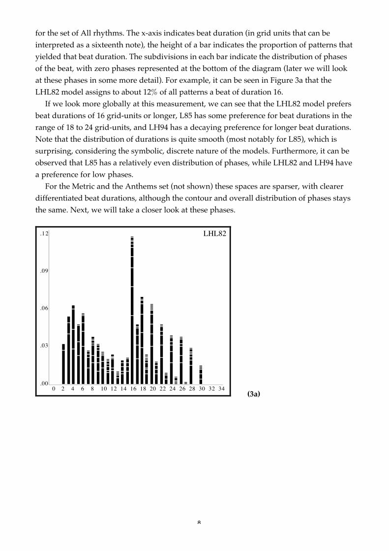
8

for the set of All rhythms. The x-axis indicates beat duration (in grid units that can beinterpreted as a sixteenth note), the height of a bar indicates the proportion of patterns thatyielded that beat duration. The subdivisions in each bar indicate the distribution of phasesof the beat, with zero phases represented at the bottom of the diagram (later we will lookat these phases in some more detail). For example, it can be seen in Figure 3a that theLHL82 model assigns to about 12% of all patterns a beat of duration 16.

If we look more globally at this measurement, we can see that the LHL82 model prefersbeat durations of 16 grid-units or longer, L85 has some preference for beat durations in therange of 18 to 24 grid-units, and LH94 has a decaying preference for longer beat durations.Note that the distribution of durations is quite smooth (most notably for L85), which issurprising, considering the symbolic, discrete nature of the models. Furthermore, it can beobserved that L85 has a relatively even distribution of phases, while LHL82 and LH94 havea preference for low phases.

For the Metric and the Anthems set (not shown) these spaces are sparser, with clearerdifferentiated beat durations, although the contour and overall distribution of phases staysthe same. Next, we will take a closer look at these phases.

0 2 4 6 8 10 12 14 16 18 20 22 24 26 28 30 32 34.00

.03

.06

.09

.12 LHL82

(3a)

9

0 2 4 6 8 10 12 14 16 18 20 22 24 26 28 30 32 34.00

.03

.06 L85

(3b)

0 2 4 6 8 10 12 14 16 18 20 22 24 26 28 30 32 34.00

.03

.06

.09 LH94

(3c)

Figure 3. Beat-space diagrams for the three models for the set of all patterns. (Proportion ofpatterns yielding a beat with a specific duration vs. beat duration counted in sixteenth-notes).

PHASE-SPACE

Phase-space diagrams depict the distribution of phases for a specific set (see Figure 4 forthe Phase-space for the set of all patterns). The x-axis indicates the phase duration (e.g. 0 isno upbeat, 2 is an upbeat of 2 grid-units), while the height of a bar indicates the proportionof a specific phase duration with respect to size of the whole pattern set.

In Figure 4 it can be seen that both LHL82 and LH94 have a clear preference for beatswith zero phase, i.e., an interpretation without upbeats. This contrasts with L85, which hasno particular preference for a particular phase. (Note that, because the beat-space was onlyanalyzed for patterns with duration of up to 35 gridunits, for L85 and LH94 the proportionof phases do not add to 1).

10

0 2 4 6 8 10 12 14 16 18 20 22 24 26 28 30 32.00

.10

.20

.30

.40

.50 LHL82

(4a)

0 2 4 6 8 10 12 14 16 18 20 22 24 26 28 30 32.00

.10 L85

(4b)

0 2 4 6 8 10 12 14 16 18 20 22 24 26 28 30 32.00

.10

.20

.30 LH94

(4c)

Figure 4. Phase-space diagrams for the three models for the set of all patterns. (Proportion ofpatterns yielding a beat with a specific phase vs. beat phase counted in sixteenth-notes).

AGREEMENT

Having shown how the overall distributions of the model’s results differ, the questionarises what the relation between is between the results of the models for a specific inputpattern? For that, patterns are taken from the sets and are categorized into four classes: the

11

class of patterns for which the three models agreed on the same beat, the three classes ofpatterns for which only two models agreed, and the class of patterns that resulted in threedifferent answers. We allowed an integer multiple of the beat duration to count as anagreed beat, provided that the phases matched as well.

The result of this measurement can be depicted in a histogram. The x-axis indicates theduration of the pattern that is used as input to the model. The height of the bar shows theproportion of patterns of that duration for which at least two models agreed. The blackpart of each bar indicates the proportion of patterns for which all three models agreed onthe beat. As an example, consider the first histogram in Figure 5. It can be seen that for allpatterns of duration 25 there is 30% agreement between all three (the black part of eachbar ), and about 85% agreement between at least two models (the total bar height).

The diagrams show in general that agreement between the three models (black part ofthe bars) increases with the amount of musical structure in the sets, up to 50% for theAnthems set. This may indicate that part of the differences of the models are exhibitedmainly when they are applied outside the domain of input patterns for which they wereconceived. Furthermore, it can be observed that the agreement between LHL82 and LH94,with L85 differing, increases with longer patterns (light gray part of the bar).

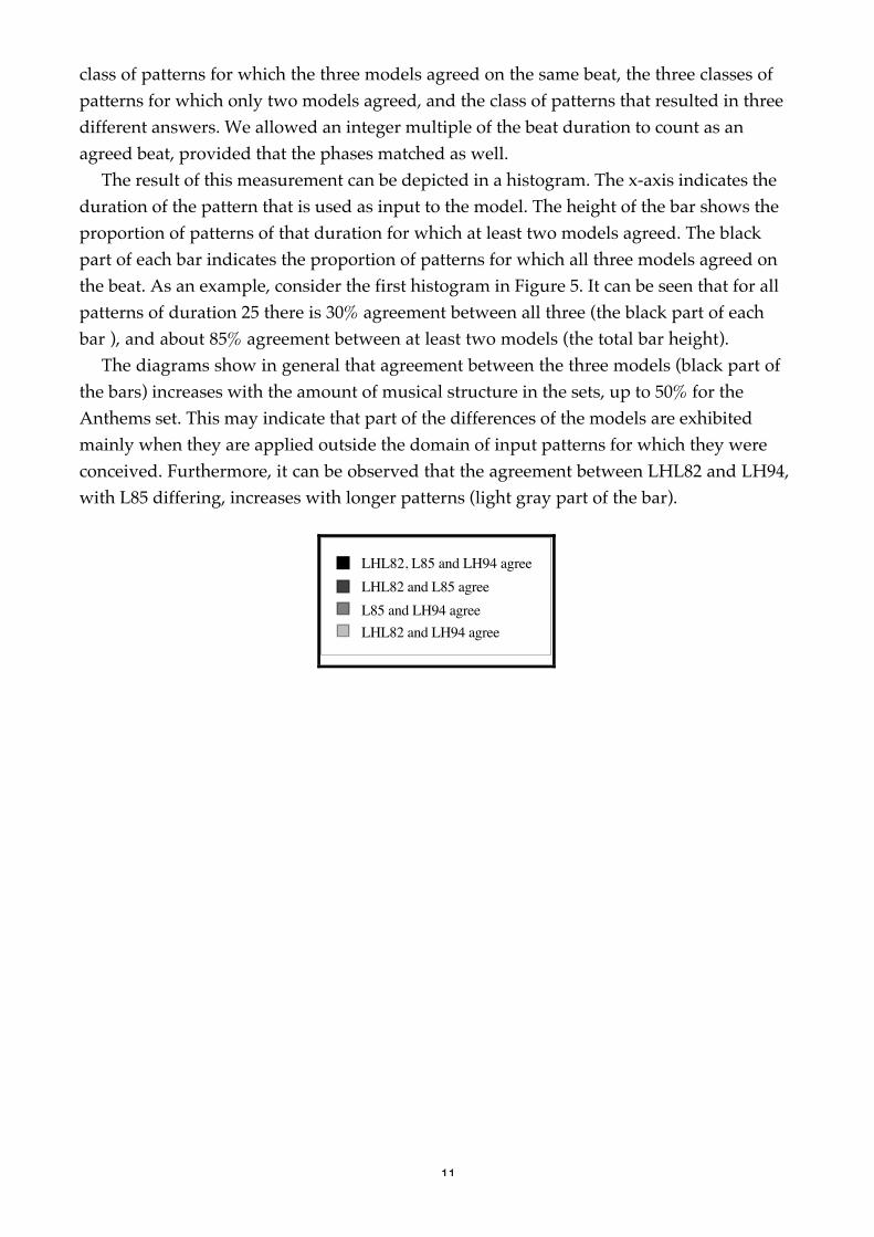
LHL82, L85 and LH94 agreeLHL82 and L85 agreeL85 and LH94 agreeLHL82 and LH94 agree

12

0 25 50 75 1000.0

0.2

0.4

0.6

0.8

1.0 All

0 25 50 75 100

0.0

0.2

0.4

0.6

0.8

1.0 Metric

0 25 50 75 1000.0

0.2

0.4

0.6

0.8

1.0 Anthems

Figure 5. Agreement diagrams for the different sets. (Proportion of pattens for which the modelsyield compatable beats vs. pattern duration counted in sixteenth-notes).

SPEED OF BEAT INDUCTION

Now we have shown how the models can arrive at the same or different answers, wecome to the question how fast these answers are arrived at. Both LHL82 and LH94 have anexplicit point at which processing stops and a result is returned. The distribution of theproportion of patterns yielding such a confirmed beat can be depicted as a function of the

13

pattern length. However, since it is quite natural to need more time to establish a longbeat, a different, and possibly fairer representation of the same data is made by expressingthe time needed for confirmation relative to the duration of the beat found. What thisanalysis (see Figure 6) shows is that, roughly spoken, both models can establish a beat of acertain duration relatively fast, on the basis of between two and three beats worth ofrhythmical material. However, in some cases LHL82 needs a much longer fragment toconfirm a beat. Here it turns out that the models clearly predict a very fast beat inductionprocess that contrasts with, for example, the much larger amount of material that coupledoscillator models (e.g., Large & Kolen, 1994) need to establish locking.

1.5 2.0 2.5 3.0 3.5 4.00. 0

0. 1

0. 2

0. 3

0. 4

0. 5 LHL82

1.5 2.0 2.5 3.0 3.5 4.00.0

0.1

0.2

0.3

0.4

0.5 LH94

Figure 6. Moment of confirmation for the sets All (black line), Metric (gray line), and Anthems(light gray line). (Proportion vs. moment of confirmation relative to the beat-length).

14

CORRECTNESS

Now we have looked at the speed at which the models arrive at an answer, we should lookat its correctness. We plan to compare the models to empirical data of human subjects, butfor some of the subsets a rough approximation of the correctness of the results can alreadybe derived. For the set of strictly metrical patterns, correct beats can be defined to be thosethat fit one of the metrical levels of one of the generating meters. For the set of nationalanthems, a correct beat can be defined as a beat that is compatible with the meter notatedin the score. For short patterns that form the beginning of more than one anthem wecounted a beat as correct whenever if fitted the meter of one of those anthems. Becausethis measure is not very stringent, it may not be valid as a judge of an absolute level ofperformance, but it can function well in comparisons between models.

The set of anthems may very well contain examples where the meter is conveyed by themelody and not by the metrical structure. In that sense the measure of correctness couldunderestimate the performance of the models, which have access to the rhythm only.

It is easy to yield small beats that conform the meter of a piece at a very low level (thesebeats are much more likely to fit than large ones, because large beats have more degreesof freedom in choosing a phase). And it is difficult to judge the merit of a beat that, thoughhaving a proper phase, spans several bars. Therefore the correctness was differentiatedaccording to the metrical level of the resulting beat.

In Figure 7 these measures are depicted as histograms. The x-axis indicates the durationof the pattern that is used as input to the model (in eighth notes). The height of the barshows the proportion of patterns that yielded a beat compatible with the notated meter ofany of the anthems starting with that pattern. The black part of each bar indicates theproportion of hyper-meter results, the beat spanning more than one measure. Below that,the dark gray area indicates the proportion of patterns that yielded a proper bar as outputof the model. The gray area below that indicates the proportion of correct beat-levelanswers, i.e. the bar divided by 2 or 3 according to the time signature. Finally, the light-gray areas indicate answers that can still be considered correct but that aligned with lowerlevels of the metrical hierarchy. As an example, consider Figure 7a in which it can be seenthat L85 rated 36% of the patterns with a duration of 24 eighth notes correctly. About 15%were rated correctly at the bar level, about 15% at the beat level, 3% above the bar leveland 3% below the beat level.

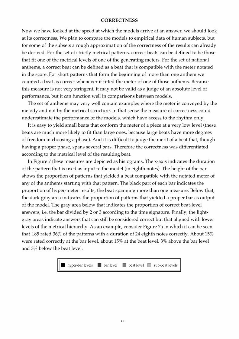
hyper-bar levels bar level beat level sub-beat levels

15

0 2 4 6 8 10 12 14 16 18 20 22 240.0

0.2

0.4

0.6

0.8 a) LHL82

0 2 4 6 8 10 12 14 16 18 20 22 240.0

0.2

0.4

0.6

0.8 b) L85

0 2 4 6 8 10 12 14 16 18 20 22 240.0

0.2

0.4

0.6

0.8 c) LH94

16

0 2 4 6 8 10 12 14 16 18 20 22 240.0

0.2

0.4

0.6

0.8 d) First-note model

0 2 4 6 8 10 12 14 16 18 20 22 240.0

0.2

0.4

0.6

0.8 e) Long-note model

0 2 4 6 8 10 12 14 16 18 20 22 240.0

0.2

0.4

0.6

0.8 f) Statistical model

Figure 7. Correct-level diagrams for the three rule-based models and three baseline models usingthe Anthems set. (Proportion of patterns yielding a correct beat vs. pattern duration counted ineighth-notes).

17

In these figures it can be seen how in subsequent stages of the processing the beathypothesis shifts upwards through the metrical levels, becoming larger and larger. Theoverall performance that the models arrive at finally is quite remarkable, considering thatin some anthems the meter might be communicated through the melodic structure,information that is ignored by these models. The LHL82 model reaches about 60% ofcorrect answers at the bar or beat level and seems to have the best performance (but seethe section on optimal parameter settings).

However, these absolute figures have to be read with caution. They have to becompared e.g. to the likelihood of arriving at a correct answer by guessing. This baselinecan easily be established by doing the same measurement for a statistical model that onlyknows the distribution of bars and beats in the total set and randomly selects a durationand a phase according to that distribution. The correctness of this model is shown in Figure7f, it forms a reference for judging the correctness of the models.

Another baseline that can be used is a model that just assumes that the first note is theproper beat. This hypothesis, which all models use initially, turns out to be not such a badone, as is shown in Figure 7d, it does yield a correct result in about 35% of the cases.However, these results only reach the beat level in 10% of the cases.

A third baseline assumes that the longest note encountered is the proper beat. And inone way or another the detection of long notes plays a crucial role in each model.However, after some initial success this strategy turns out to be quite unsuccessful, it evenperforms below chance level, as can be seen in Figure 7e.

RULE CALLS

Before studying the contribution of the individual rules to the model’s performance oneneeds to check how often the different rules fire? In Figure 8 the proportion of cases inwhich each rule fires is given for each model and each set.

It can be seen how the LHL82 LONGNOTE rule applies relatively infrequent comparedto the other rules (LONGNOTE fires when a note is longer than twice the current beat).The STRETCH rule, in which a long note is encountered that does not align with the beat,applies more often while processing random rhythms than in the structured sets.Conversely, the CONFLATE rule, that fires whenever a note is encountered on a next beat,is more often called in the Metric and the Anthems set. Both results confirm the expectationabout the amount of musical structure in the different sets.

18

STRETCHUPDATECONFLATELONGNOTE STRETCHUPDATE

0.0

0.2

0.6

0.8

1.0

0.4

STRETCHUPDATECONFLATE

0.0

0.2

0.6

0.8

1.0

0.4

0.0

0.2

0.6

0.8

1.0

0.4

LHL82 L85 LH94

Anthems

Metric

All

Figure 8. Proportion of rule calls for the three models for the set of all patterns (top), theMetric set (middle), and the Anthems set (bottom).

ROBUSTNESS

After we know how often the rules are applied, it can be questioned how crucial theapplication of a rule’s action is when its matching pattern is encountered in the input. It canbe argued that meaningful musical material does contain many redundant cues to themeter (as can be experienced when tuning the radio and finding oneself suddenly listeningto the middle section of an anthem), and the system might get a second chance at getting itright. This issue was resolved in the form of a measurement that gave one rule a change ofnot firing in a situation where it otherwise would. In Figure 9 the resulting performance(the proportion of correct answers at the bar or beat level) is given as a function of thechance that a rule fires when it should. The correctness measurement was taken at the

19

point where processing stopped, this is why the level of correctness when all rules fire asthey should (at 1.0) cannot be directly compared to the final correct proportion at the barand beat level in Figure 7a, 7b and 7c.

STRETCH LONGNOTE UPDATE CONFLATE

0.0 0.2 0.4 0.6 0.8 1.00.0

0.2

0.4

0.6

0.8

1.0 LHL82

0.0 0.2 0.4 0.6 0.8 1.0

0.0

0.2

0.4

0.6

0.8

1.0 L85

0.0 0.2 0.4 0.6 0.8 1.00.0

0.2

0.4

0.6

0.8

1.0 LH94

Figure 9. Robustness for the three models for the Anthems set. (Proportion of patterns yielding acorrect beat vs. application probability of each rule).

It turns out that all three model behave quite robustly under this condition, even in caseof the complete removal of a rule. Overall, there seem to be multiple cues in the music thatallow a later repair of the situation caused by a broken rule. This holds especially for theCONFLATE rule which can double the beat. Furthermore, it can be observed thatSTRETCH has quite an important role in both LHL82 and LH94. Remarkably, theperformance of L85 improves when the STRETCH and the UPDATE rule are not always

20

used. And indeed L85 seems to take long notes too seriously and often changes the beat ata syncopation.

EFFECTIVENESS OF THE RULES

We will continue focussing in more and more on the rules themselves and next address thequestion how beneficial the actions of the different rules are when they fire. This wasmeasured by counting the cases in which a rule succeeds in repairing a wrong beat, i.e. thebeat being wrong just before and correct (at any level) just after the application of a rule.This number can then be compared to the number of cases in which a rule’s action breaksthe beat, i.e. it was correct before and wrong after application. In Figure 10 the proportionof these cases is shown for each rule (given that it fires). Both the INITIALIZE andCONFIRM rule are not depicted in Figure 10. The former because it invariably repairs anon-existing beat hypothesis into a correct one in 70% of the cases, the latter because itdoesn’t alter the beat hypothesis, and therefore it never breaks nor repairs.

It can be seen that the STRETCH rule does a good job in repairing wrong beathypotheses. The UPDATE rule in LH82 never breaks or repairs the beat since it simplyshifts the beat. The absence of a rating for LONGNOTE in LH82 is due to an artifact in ourmeasurement procedure. The large proportion of cases in which the UPDATE rule breaks acorrect beat hypothesis in model LH94 is puzzling and topic of further study.

Break Repair

STRETCH

UPDATE

LONGNOTE

CONFLATE

0.2 0 0.2 0.4 0.6

LHL82

21

STRETCH

UPDATE

0.2 0 0.2 0.4 0.6

L85

STRETCH

UPDATE

CONFLATE

0.2 0 0.2 0.4 0.6

LH94

Figure 10. Effectiveness of the rules for the three models for the Anthems set. (Rule vs.proportion of rule calls that are breaks and repairs of the current beat hypothesis).

IS THERE A BEST UPDATE RULE?

In the models three different UPDATE rules are used. The UPDATE rule is intended to skipover upbeats. All UPDATE rules fire whenever they encounter a relatively long note(under specific conditions) in the input. But all models apply a different action in that case.LHL82 shifts the beat, maintaining its duration. The LH94 model shifts and elongates thebeat to the onset of the next note. The L85 model shifts and elongates the beat to the onsetof the next note that happens to fall on a beat. These actions are illustrated in Figure 11. Itshows an example pattern (a line is a note onset, the curves indicate the beats) before theUPDATE rule fires, and the situation after it has done its action.

22

LHL82

L85

LH94

| . . | . . . | . !

after UPDATE

before UPDATE

Figure 11. Definitions of the UPDATE rule.

To test the different UPDATE rules, we transplanted the different variants into the threemodels. Because in LHL82 the function of the UPDATE rule is closely intertwined with theLONGNOTE rule, it was transplanted both with and without the LONGNOTE rule to theother two models. In two cases the transplanted LONGNOTE rule was made inoperativeby the rest of the rule set (the UPDATE rule from L85 makes the beat so long thatLONGNOTE never applies anymore). These combinations were eliminated. The resultingrule cocktails were all tested for correctness, measuring at the point of confirmation forLHL82 en LH94 and at the end of the anthem for L85. The results are given in Figure 12,with the subdivisions of the bars as used in the figures for the Correct-level analysis: blackis above, dark gray on and gray just below the bar level (i.e. beat level), light gray beingthe correct answers below the beat level.

The results are aligned such that the proportions can be compared per rule-cocktail forthe beat and bar levels (gray and dark gray). The correctness at the sub-beat levels (lightgray) and hyper-bar levels (black) constitute less useful answers.

23

L85 + LONGNOTE + UPDATE-LHL82

L85 + UPDATE-LH94

L85 + UPDATE-LHL82

0 0.1 0.2 0.3 0.4 0.5 0.6 0.7

LH94

LH94 + UPDATE-L85

LH94 + UPDATE-LHL82

LH94 + LONGNOTE + UPDATE-LHL82

L85

LHL82

LHL82 + UPDATE-LHL82

LHL82 + UPDATE-LH94

LHL82 + UPDATE-L85

0.1

hyper-bar levels

beat levelbar level

sub-beat levels

Figure 12. Correctness of the rule-cocktails and the original models for the Anthems set. (Proportionof patterns yielding a correct beat vs. rule cocktails).

In Figure 12 we can see that LHL82 obtains the best score (i.e. 55% correct at the beatand bar level), followed by LHL82 with the UPDATE rule form LH94. No differencebetween the performance of LH94 and of the LH94 model with a transplanted UPDATE enLONGNOTE rule from LHL82. However, these results were calculated with the parametersettings supplied by the author, and different settings yield a different result, as will beshown next.

WHAT ARE THE OPTIMAL PARAMETER SETTINGS?

Finally, we will use the correctness analysis (considering only bar and beat level answers ascorrect) to search for the optimal parameter setting of the models, i.e. the setting thatproduces the highest proportion of correct results.

We will show here the results for the LHL82 and LH94 model (the L85 model has noparameters). In Figure 13 the performance of the models is shown as function of theirparameters. The LHL82 model, which was described in the literature with an unformalized“near-beginning” predicate that controlled whether the update rule is still allowed to fire,was augmented with an update-interval parameter that specified this point in time.

24

maximum-beatupdate-

interval

corre

ct fr

actio

n

16 18 20 22 24 26 28 30 32 34 36 38

0

8

16

24

0

0.1

0.2

0.3

0.4

0.5

0.6

0.7

0.8

LHL82

2 3 4 5 6 7 8 9 10 11 12 13 14 15 160

4

120

0.1

0.2

0.3

0.4

0.5

0.6

0.7

0.8

minimum-beat

maximum-updatable-b

eat

corre

ct fr

actio

n

8

LH94

Figure 13. Parameter-spaces for the Anthems set (gray = original setting, black = optimal setting).(Proportion of patterns yielding a correct beat vs. parameter values).

The LHL82 model achieves an optimal performance with the maximum-beat parameter,which controls whether beats may still be conflated, set around 20 sixteenth notes. The

25

original setting of this parameter is 30 sixteenth notes. The update-interval parameter,which controls until when the UPDATE rule still allowed to fire, should be set around 16sixteenth notes for optimal performance. No value was specified for this parameter in theoriginal model. The optimal performance level then rises to about 60 % correct at the baror beat level. The LH94 model yields its best performance with the minimum-beatparameter, which prohibits the confirmation of small beats, set at 6 sixteenth notes. Itsoriginal setting was 8 sixteenth notes. The maximum-updatable-beat parameter, controllinguntil when the UPDATE rule still is allowed to fire, which was originally set to 4 sixteenthnotes, is optimal at 6 sixteenth notes. The level then rises to 80 % correct, which makes thismodel an improvement indeed.

CONCLUSION AND FUTURE RESEARCH

We also hope to have shown that these methods are a promising way of characterizing thebehavior of computational models of beat induction. Using these methods we were able toanswer a set of questions that could not have been addressed otherwise. Differences inpreferred beat duration and phase between the models were shown - with the L85 modelallowing for much longer upbeats. It was illustrated how the amount of agreement oninduced beat increased with the amount of musical structure in the test set used. The(amazingly short) time needed by the models to establish a beat was estimated to be aboutthree beat-lengths of musical material. After that time the LHL82 model arrived for 70% ofthe cases at a beat answer that was compatible with the time signature notated in the scoreof the anthems, the other models performing worse. But, all models behave quite robustlywhen one of their components is made partly inoperative, which is surprising for rulebased systems. The variants of the UPDATE rule proved not to be easily cross-transplantedwithout loss of performance. However, a large gain in performance (almost doubling thepercentage of correct answers) proved obtainable by optimizing the parameter settings ofthe LHL82 and the LH94 model.Our plans for the future are to apply the same methodology to families of models that arebased on alternative formalisms. Furthermore, we plan to elaborate a perceptual measureof correctness that is based directly on empirical data. After a further round offormalization we will attempt to generalize the idea of rule cocktails to systems that havetheir rules specified in the form of a formal pattern-matching language, such that themembers of this family may be enumerated and tested, possibly using genetic algorithms.The rule-based models, even though they are simple and ignore effects like tempo, timing,melody and harmony, turn out behave surprisingly well.

26

ACKNOWLEDGMENTS

Special thanks to Christopher Longuet-Higgins for his contribution in several discussions,and providing access to his programs. Part of this work was done while visiting CCRMA,Stanford University on kind invitation of Chris Chafe and John Chowning, supported by atravel grant of the Netherlands Organization for Scientific Research (NWO). The researchhas been made possible by a fellowship of the Royal Netherlands Academy of Arts andSciences (KNAW).

REFERENCES

Desain, P. & H. Honing (1994a). A brief introduction to beat induction In Proceedings of the1994 International Computer Music Conference. 78-79. San Francisco: InternationalComputer Music Association.

Desain,P. & H. Honing (1994b). Rule-based models of initial beat induction and an analysisof their behavior. In Proceedings of the 1994 International Computer Music Conference. 80-82. San Francisco: International Computer Music Association.

Desain,P. & H. Honing (1995). Computational Models of Beat Induction: The Rule-basedApproach. In G. Widmer (ed.), Working Notes: Artificial Intelligence and Music. 1-10.Montreal: IJCAI.

Essens, P. (1995). Structuring Temporal Sequences: Comparison of Models and Factors ofComplexity. Perception & Psychophysics. 57(4), 519-532.

Large, E. W. & J. F. Kolen (1994). Resonance and the perception of musical meter.Connection Science, 6 (1), 177-208.

Lee, C. S. (1985). The rhythmic interpretation of simple musical sequences: towards aperceptual model. In R. West, P. Howell, & I. Cross (eds.) Musical Structure andCognition. 53-69. London: Academic Press.

Lee, C. S. (1991). The perception of metrical structure: Experimental evidence and a model.In P. Howell, R. West, & I. Cross (Eds.), Representing musical structure . 59-127. London:Academic.

Longuet-Higgins, H. C. & C. S. Lee (1982). Perception of musical rhythms. Perception. 11,115-128.

Longuet-Higgins, H. C. (1994). Unpublished computer program in POP-11, describing analgorithm named “shoe”.

Miller, B. O., D. L. Scarborough, & J. A. Jones (1992) On the perception of meter. In M.Balaban, K. Ebcioglu, & O.Laske (eds.), Understanding Music with AI: Perspectives onMusic Cognition. 428- 447. Cambridge: MIT Press.

Shaw, M. and H. Coleman (1960) National Anthems of the World. London: Pitman.