Computational models of long term plasticity and memory ∗

Stefano FusiCenter for Theoretical Neuroscience, College of Physicians and Surgeons, Columbia University

Mortimer B. Zuckerman Mind Brain Behavior Institute, Columbia University

Kavli Institute for Brain Sciences, Columbia University

June 16, 2017

1 Introduction

Memory is often defined as the mental capacity of retaining information about facts, events, proceduresand more generally about any type of previous experience. Memories are remembered as long asthey influence our thoughts, feelings, and behavior at the present time. Memory is also one of thefundamental components of learning, our ability to acquire any type of knowledge or skills.

In the brain it is not easy to identify the physical substrate of memory. Basically, any long-lastingalteration of a biochemical process can be considered a form of memory, although some of thesealterations last only a few milliseconds, and most of them, if taken individually, cannot influence ourbehavior. However, if we want to understand memory, we need to keep in mind that memory is nota unitary phenomenon, and it certainly involves several distinct mechanisms that operate at differentspatial and temporal levels.

One of the goals of theoretical neuroscience is to try to understand how these processes are orches-trated to store memories rapidly and preserve them over a lifetime. Theorists have mostly focused onsynaptic plasticity, as it is one of the most studied memory mechanisms in experimental neuroscienceand it is known to be highly effective in training artificial neural networks to perform real world tasks.Some of the synaptic plasticity models are purely phenomenological and they have proved to be im-portant for describing quantitatively the complex and rich observations in experiments on synapticplasticity. Some other models have been designed to solve computational problems, like pattern clas-sification, or simply to maximize the memory capacity in standard benchmarks. Finally, there aremodels are inspired by biology, but then find an application to a computational problem, or vice versa,there are models that solve complex computational problems that then are discovered to be biologicallyplausible. In this article I will review some of these models and I will try to identify computationalprinciples that underlie memory storage and preservation (see also [Chaudhuri and Fiete, 2016] for arecent review that focuses on similar issues).

2 Long term synaptic plasticity

2.1 Abstract learning rules and synaptic plasticity

Artificial neural networks are typically trained by changing the parameters that represent the neuronalactivation thresholds and the synaptic weights that connect pairs of neurons. The algorithms used to

∗draft of an article that is being considered for publication by Oxford University Press in the forthcoming book ”OxfordResearch Encyclopedia of Neuroscience”, Editor S. Murray Sherman, due for publication in 2017.

1

arX

iv:1

706.

0494

6v1

[q-

bio.

NC

] 1

5 Ju

n 20

17

train them can be divided into three main groups (see e.g. a classic textbook like [Hertz et al., 1991])1) networks that are able to create representations of the statistics of the world in an autonomous way(unsupervised learning) 2) networks that can learn to perform a particular task when instructed by ateacher (supervised learning) 3) networks that can learn by a trial and error procedure (reinforcementlearning). These categories can have a different meaning and different nomenclature depending onthe community (machine learning or theoretical neuroscience). For all these algorithms, memory is afundamental component which typically resides in the pattern of synaptic weights and in the activationthresholds. Every time these parameters are modified, the memory is updated.

2.1.1 The perceptron

Rosenblatt [Rosenblatt, 1958, Rosenblatt, 1962] introduced in the 60’s one of the fundamental algo-rithms for training neural networks. He studied in detail what is probably the simplest feed-forwardneural ’network’, and the fundamental building block of more complex networks. He called it theperceptron. The perceptron is just one output neuron that is connected to N input neurons. For agiven input pattern xµ (xµ is a vector, and its components xµi s are the activation states of specificneurons), the total current into the output neuron is a weighted sum of the inputs:

Iµ =N∑i=1

wixµi

The output neuron can be either active or inactive. It is activated by the input only when I isabove an activation threshold θ.

The learning algorithm is supervised and it can be used to train the perceptron to classify inputpatterns into two distinct categories. During learning, the synaptic weights and the activation thresholdare tuned so that the output neuron responds to each input as prescribed by the supervisor. Forexample, consider the classification problem in which the inputs represent images of handwrittendigits and the perceptron has to decide whether a digit is odd or even. During training the perceptronis shown a large number of samples of odd and even digits, and the output neuron is set by thesupervisor to the activation state corresponding to the class to which the input belongs (e.g. theneuron is activated when the digit is odd, inactivated when it is even).

The learning procedure ensures that after learning the perceptron responds to an input as prescribedby the supervisor, even in its absence. The input can be one of the samples used for training, or anew sample from a test set. In the second case the perceptron is required to generalize and classifycorrectly also the new inputs (e.g. a new handwritten digit).

The proper weights and the threshold are found using an iterative algorithm: for each input pattern,there is a desired output provided by the supervisor, which is yµ (yµ = −1 for input patterns thatshould inactivate the output neuron and yµ = 1 for input patterns that should activate the outputneuron), and each synapse wi, connecting input neuron i to the output is updated as follows:

wi → wi + αxµi yµ (1)

where α is a constant that represents the learning rate. The threshold θ for the activation of theoutput neuron is modified in a similar way:

θ → θ − αyµ

The synapses are not modified if the output neuron already responds as desired. In other words,the synapse is updated only if the total synaptic current Iµ is below the activation threshold θ whenthe desired output yµ = +1 (and analogously when Iµ > θ and yµ = −1). The synapses are updated

2

for all input patterns, repeatedly, until all the conditions on the output are satisfied. These synapticupdates are a simple form of synaptic plasticity.

The importance of the perceptron algorithm resides in the fact that it can be proved [Block, 1962]to converge if the patterns are linearly separable (i.e. if there exists a wi and a threshold θ such thatIµ > θ for all µ such that yµ = 1 and Iµ < θ for all µ such that yµ = −1). In other words, if asolution to the classification problem exists, the algorithm is guaranteed to find one in a finite numberof iterations. The convergence proof is probably one of the earliest elegant results of computationalneuroscience.

2.1.2 Hebb’s principle

The perceptron algorithm is also considered one of the early implementations of Hebb’s principle[Hebb, 1949]. The principle reflects an important intuition of Donald Hebb about a basic mechanismfor synaptic plasticity. It states:

“When an axon of cell A is near enough to excite a cell B and repeatedly or persistently takes partin firing it, some growth process or metabolic change takes place in one or both cells such that A’sefficiency, as one of the cells firing B, is increased.”

The efficiency he refers to can be interpreted as the synaptic efficacy, or the weight wi that we definedabove. The product of the activities of pre and post-synaptic neurons that appear in the synapticupdate equation Eq.1 is often considered an expression of the Hebbian principle: when the inputand the output neuron (pre and post-synaptic, respectively) are simultaneously active, the synapse ispotentiated. In the case of the perceptron, the output neuron is activated by the supervisor duringtraining and it reflects the desired activity.

2.1.3 Extensions of the perceptron algorithm

Synaptic models that are biologically plausible implementations of the perceptron algorithms have beenproposed in the last decades (see e.g.[Brader et al., 2007, Legenstein et al., 2005a]). In these modelsthe neuronal activity is often expressed as the mean firing rate, but there are models that consider thetiming of individual spikes. An interesting class of spike driven synaptic models solves the computa-tional problem of how to train neurons to classify spatio-temporal patterns of spikes. For example, thetempotron algorithm, introduced by Gutig and Sompolinsky in 2006 [Gutig and Sompolinsky, 2006],can be used to train a spiking neuron to respond to a specific class of input patterns by firing atleast once during a given time interval. The neuron remains silent in response to all the other inputpatterns. A recent extension of the model can be trained to detect a particular clue (basically a specificspatio-temporal pattern) simply by training it to fire in proportion to the clue’s number of occurrencesduring a particular time interval [Gutig, 2016].

Besides the perceptron, there are other learning algorithms that are based on similar principlesand often the synaptic weights are modified on the basis of the covariance between the pre and postsynaptic activity (see e.g. [Sejnowski, 1977, Hopfield, 1982]). Many of these algorithms can be derivedfrom first principles, for example by minimizing the error of the output.

Error minimization is also the basic principle of a broad class of learning algorithms that can trainartificial neural networks that are significantly more complex than the perceptron. For example feed-forward networks with multiple layers (deep) can be trained by computing the error at the outputand backpropagating it to all the synapses of the network. This algorithm, called backpropagation[Rumelhart et al., 1986], has recently revolutionalized machine vision, and is extremely popular inartificial intelligence [LeCun et al., 2015]. Although it is difficult to imagine how backpropagation canbe implemented in a biological system, several groups are working on versions of the algorithm whichare more biological plausible (see e.g.[Lillicrap et al., 2016, Scellier and Bengio, 2016]). In the future

3

these models will certainly play an important role in understanding synaptic dynamics and learning inthe biological brain.

2.2 Phenomenological synaptic models

The synaptic models mentioned in the previous section were designed to implement a specific learningalgorithm. However, there are also several models that were initially conceived to describe the richphenomenology observed in experiments on synaptic plasticity.

A popular class of models was inspired by the experimental observations that long term synapticmodifications depend on the precise timing of pre- and post-synaptic spikes[Levy and Steward, 1983,Markram et al., 1997, Bi and Poo, 1998, Sjostrom et al., 2001]. These models are usually describedusing the acronym STDP (Spike Timing Dependent Plasticity), introduced by Larry Abbott and col-leagues to designate a specific model[Song et al., 2000]. In the simplest version of STDP, when the pre-synaptic spike precedes a post-synaptic spike within a time window of 10-20 ms, the synapse is poten-tiated and for the reverse order of occurrence of pre and post-synaptic spikes, the synapse is depressed.Phenomenological models can describe accurately many other aspects of the experimental observations[Senn et al., 2001, Pfister and Gerstner, 2006, Morrison et al., 2008, Clopath et al., 2010]. Several the-oretical studies describe the dynamics of neural circuits whose synapses are continuously updated usingSTDP[Song et al., 2000, Song and Abbott, 2001, Babadi and Abbott, 2010, Babadi and Abbott, 2013].The role of STDP in learning has also been investigated in many computational studies (see e.g.[Gerstner et al., 1996, Legenstein et al., 2005b, Gutig and Sompolinsky, 2006, Izhikevich, 2007, Legenstein et al., 2008,Nessler et al., 2013, Pecevski and Maass, 2016]). One of the theoretical works [Gerstner et al., 1996]preceded the experimental papers on STDP and hence predicted the STDP observations.

Although the computational principles behind STDP are probably general and important, exper-iments on synaptic plasticity show that STDP is only one of the aspects of the mechanisms for theinduction of long term changes (see e.g. [Shouval et al., 2010]). The direction and the extent of asynaptic modification depend on various types of ’activity’ of the pre and post-synaptic neurons (notonly on spike timing), on the location of the synapses on the dendrite [Sjostrom and Hausser, 2006],on neuromodulators [Squire and Kandel, 1999, Sjostrom et al., 2008], on the timescales that are con-sidered in the experiment (e.g. homeostatic plasticity occurs on timescales that are significantly longerthan those of long term synaptic plasticity[Turrigiano and Nelson, 2004]) and, most importantly, onthe history of previous synaptic modifications, a phenomenon called meta-plasticity [Abraham, 2008](see also below).

A recent synaptic model can reproduce part of the rich STDP phenomenology observed in multipleexperiments using a surprisingly small number of dynamical variables which include calcium concen-tration [Graupner and Brunel, 2011] (see Fig. 2.2 for a description of the model and an explanationof how it can reproduce STDP).

3 Memory

The synaptic plasticity models described in the previous section can predict to some extent the signof the synaptic modification. However, these models focus on one of the early phases of synaptic plas-ticity. The consolidation and the maintenance of synaptic modifications require a complex molecularmachinery that typically involves cascades of biochemical processes that operate on different timescales.Typically the process of induction of long term synaptic modifications starts with an alteration of someof the molecules that are locally present at the synapse. For example, in Fig. 2.2 we described a modelin which calcium concentration increases at the synapse at the arrival of either the pre-synaptic spike orthe post-synaptic back propagating action potential. The entry of calcium then induces an alterationof the state of some relatively complex molecules that are locally present, like the calcium/calmodulin

4

c(t)

LTD LTP(a) (b)

(d)(c)

D

D

θ+θ-

Figure 1: Calcium based synaptic model proposed in [Graupner and Brunel, 2011]: long term depression (LTD,left) and long term potentiation (LTP, right). The spike timing dependent plasticity (STDP) protocol forinducing long term modifications are illustrated at the top in panels (a) and (b): when the post-synaptic spikeprecedes the pre-synaptic spike, LTD is induced. The synapse is modified in the opposite direction (LTP) whenthe pre-synaptic spike precedes the post-synaptic action potential. This dependence of the sign of the synapticmodification on the relative timing of pre and post synaptic spikes can be obtained by introducing an internalvariable that represents the post-synaptic calcium concentration c(t). The weight increases when c is above athreshold θ+ (orange in the figure) and it decreases when c is between θ− (cyan) and θ+. The calcium variablejumps to a higher value every time a pre-synaptic or a post-synaptic spike arrives. It does so instantaneouslyfor post-synaptic spikes, and with a delay D ∼ 10ms for pre-synaptic spikes. It then decays exponentially witha certain time constant, of the order of a few ms. In panels (c) and (d), c(t) is plotted as a function of timein the LTD and LTP protocols based on STDP. When the post-synaptic spike precedes the pre-synaptic one,the calcium variable c(t) spends more time between the orange and the cyan lines than above the orange line,eventually inducing long term depression (panel (c)). When the pre-synaptic spike precedes the post-synapticaction potential (panel (d)), most of the time the calcium variable is above the orange line and LTP is induced.Figure adapted from [Graupner and Brunel, 2011].

dependent protein kinase II (CaMKII). In the case of CaMKII, each molecule can be either phospho-rylated (activated) or unphosphorylated (inactived) and hence it can then be considered as a simplememory switch. The population of the few (5-30) CaMKII molecules that are present and immobilizedin a dendritic spine are a basic example of a molecular memory. Their state modulates the strength ofthe synaptic connection.

One of the problems of molecular memories is related to their stability. Because of molecularturnover (see e.g.[Crick, 1984]), the memory molecules are gradually destroyed and replaced by newlysynthesized ones. To preserve the stored memories, the state of the old molecules should be copied tothe incoming naive ones. If not, the memory lifetime is limited by the lifetime of the molecule, which,in the case of CaMKII is of the order of 30 hours. Other molecules can last longer, but none of them cansurvive a lifetime. One possible explanation for long memory lifetimes is bistability, which was alreadyproposed by Francis Crick [Crick, 1984]. For example, in the case of CaMKII one can imagine that thepopulations of all molecules has two stable points: one in which none of the molecules is active, andanother one in which a large proportion is active. The dynamics of models describing this form of bista-bility have been studied in detail [Lisman, 1985, Lisman and Zhabotinsky, 2001, Miller et al., 2005a].When a new inactivated protein comes in, it remains unaltered if the majority of the existing CaMKII

5

molecules are inactivated, and it is activated if they are in the active state. As a consequence, the newmolecules can acquire the state of the existing ones, preserving the the molecular memory at the levelof the population of CaMKII molecules.

CaMKII is only one of the numerous molecules that are involved in synaptic plasticity: morethan 1000 different proteins have been identified in the post synaptic proteom of mammalian brainexcitatory synapses (see e.g. [Emes and Grant, 2012]). Interestingly, less than 10% of these proteinsare neurotransmitter receptors, which suggests that the majority of proteins are not directly involvedin electrophysiological functions and instead have signaling and regulatory roles. CaMKII is knownto be important in the early phases of the induction of long term synaptic potentiation (E-LTP).The molecules involved in E-LTP activate a cascade of biochemical processes that eventually regulategene transcription and protein synthesis, leading to permanent changes in the morphology of thesynaptic connections or to persistent molecular mechanisms that are known to underlie late long termpotentiation (L-LTP) maintenance. The foundational work on these cascades of biochemical processesof Eric Kandel and colleagues is summarized in [Squire and Kandel, 1999].

To understand the computational role of these highly organized protein networks, it is necessary toreview more than 30 years of theoretical studies. The next sections summarize some of the importantresults of these studies that show that biological complexity plays a fundamental role in maximizingmemory capacity.

3.1 Memory models and synaptic plasticity

For many years, research on the synaptic basis of memory focused on the long-term potentiation ofsynapses which, at least by the modeling community, was represented as a simple switch-like changein synaptic state. Memory models studied in the 1980s (i.e. [Hopfield, 1982]) suggested that networksof neurons connected by such switch-like synapses could maintain huge numbers of memories virtuallyindefinitely. Although it becomes progressively more difficult to retrieve memories in these models astime passes and additional memories are stored, the memory traces of old experiences never fade awaycompletely (see e.g. [Amit, 1989, Hertz et al., 1991]. Memory capacity, which was computed to beproportional to network size, was only limited by interference from multiple stored memories, whichcan hamper memory retrieval. This work made it appear that extensive memory performance couldarise from a relatively simple mechanism of synaptic plasticity. However, it was already clear fromthe experimental works summarized above that synaptic plasticity is anything but simple. If, as thetheoretical work suggested, this complexity is not needed for memory storage, what is there for?

The key to answering this question arose from work done at the beginning of the 90s. Thiswork arose from a project led by D. Amit aimed at implementing an associative neural network inan electronic chip using the physics of transistors to emulate neurons and synapses, as originallyproposed by Carver Mead [Mead, 1990]. The main problem encountered in this project was relatedto memory. The problem was not how to preserve the states of synapses over long times, but howto prevent memories from being overwritten by other memories. Memories were overwritten by othermemories so rapidly that it was practically impossible for the neural network to store any information.Subsequent theoretical analysis of this problem [Amit and Fusi, 1992, Amit and Fusi, 1994, Fusi, 2002,Fusi and Abbott, 2007] showed that what had appeared to be a simple approximation made in thetheoretical calculations of the 80s was actually a fatal flaw. The unfortunate approximation wasignoring the limits on synaptic strength imposed on any real physical or biological device. When theselimits are included, the memory capacity grows only logarithmically rather than linearly with networksize, and the models could no longer account for actual biological memory performance.

6

100 101 102 103 104 105 106 107

Number of memories

100

101

102

103

104S

NR

Bidirectional cascadeCascade modelFast bistable syn.Slow bistable syn.Heterogeneous 1/t

Heterogeneous 1/t 1/2

Minute Hour Day Month Year DecadeCentury

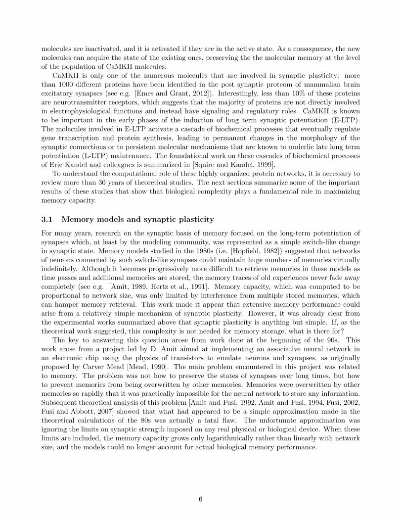
Figure 2: Memory trace (signal to noise ratio, or SNR) as a function of time (i.e. the age of thetracked memory) for four different models. The dashed line is an arbitrary threshold for memoryretrieval: memories are basically forgotten when SNR drops below this threshold. Dark red line: fastsimple bistable synapses (all synapses have q near 1). The initial memory trace is large, but thedecay is rapid. Light red line: slow simple bistable synapses (all synapses have small q ∼ 1/

√N):

long memory lifetime but small initial memory trace. Purple: cascade model, with a large initialmemory trace, power law decay (1/t), and long memory lifetimes. Black: bidirectional cascade model:power law decay (1/

√t) and the initial memory trace is as large as for the cascade model. Light

and dark green: heterogeneous population of simple bistable synapses. Light green: synapses aredivided in 20 equal size subpopulations, each characterized by a different value of the learning rate q(q = 0.6(k−1), k = 1, ..., 20). The SNR decays as 1/t and the scaling properties are the same as for thecascade model. Dark green: same number of subpopulations, but now their size increases as q becomessmaller (the size is proportional to 1/

√q). The decay is slower (1/

√t) compared to the heterogeneous

model with equal size subpopulations, however the initial SNR is strongly reduced as it scales as N1/4.For this model the memory lifetime scales as

√N . To give an idea of the timescales that might be

involved, for all curves we assumed that new uncorrelated memories are stored at the arbitrary rate ofone every minute.

7

3.2 The plasticity-stability tradeoff

In discussing the capacity limitations of any memory model, it is important to appreciate a tradeoff be-tween two desirable properties, plasticity and stability [Carpenter and Grossberg, 1991]. To reflect thistradeoff, we characterize memory performance by two quantities [Fusi et al., 2005, Fusi and Abbott, 2007,Benna and Fusi, 2016, Arbib and Bonaiuto, 2016]. One is the strength of the memory trace right aftera memory is stored. This quantity reflects the degree of plasticity in the system, that is its ability tostore new memories. The other quantity is memory lifetime, which reflects the stability of the systemfor storing memories over long times.

To better understand the trade-off it is important to define more precisely what we mean by memorystrength. In the standard memory benchmark, the strength of a particular memory trace is estimatedin a particular situation in which memories are assumed to be random and uncorrelated. One of thereasons behind this assumption is that it allowed theorists to perform analytic calculations. However,it is a reasonable assumption even when more complex memories are considered. Indeed, storage ofnew memories is likely to exploit similarities with previously stored information (consider e.g. semanticmemories). Hence the information contained in a memory is likely to be preprocessed, so that onlyits components that are not correlated with previously stored memories are actually stored. In otherwords, it is more efficient to store only the information that is not already present in our memory. Asa consequence, it is not unreasonable to consider memories that are unstructured (random) and do nothave any correlations with previously stored information (uncorrelated).

3.2.1 Memory traces: signal and noise

Consider now an ensemble of N synapses which is exposed to an ongoing stream of random anduncorrelated modifications, each leading to the storage of a new memory defined by the pattern of Nsynaptic modifications potentially induced by it. One can then select arbitrarily one of these memoriesand track it over time. The selected memory is not different or special in any way, so that the resultsfor this particular memory apply equally to all the memories being stored.

To track the selected memory one can take the point of view of an ideal observer that knows thestrengths of all the synapses relevant to a particular memory trace [Fusi, 2002, Fusi et al., 2005]. In thebrain the readout is implemented by complex neural circuitry, and the strength of the memory tracebased on the ideal observer approach may be significantly larger than the memory trace that is actuallyusable by the neural circuits. However, given the remarkable memory capacity of biological systems, itis not unreasonable to assume that the readout circuits perform almost optimally. Moreover, there aresituations in which the ideal observer approach predicts the correct scaling properties of the memorycapacity of simple neural circuits that actually perform memory retrieval.

More formally we define the memory signal of a particular memory that was stored at time tµ asthe overlap (or similarity) between the pattern of synaptic modifications ∆wi imposed by the eventand the current state of the synaptic weights wi at time t:

Sµ(t) ≡ 1

N

⟨ N∑i=1

wi(t) ∆wi(tµ)⟩.

Angle brackets indicate an average over the random uncorrelated patterns that represent the othermemories and that make the trace of the tracked memory noisy. The noise is just the standarddeviation of the overlap that defines the signal:

Nµ(t) ≡

√√√√ 1

N2

⟨( N∑i=1

wi(t) ∆wi(tµ))2⟩− Sµ(t)2 .

8

The quantity gives the strength of the trace of memory µ will then be S/N , the signal to noise ratio(SNR) of a memory.

3.2.2 The initial signal to noise ratio: plasticity

The initial SNR is then the SNR of a memory immediately after it has been stored, when it is mostvivid. Highly plastic synapses allow for large initial SNR. Typically, in many realistic models, the SNRdecreases with the memory age, so the initial SNR is often the largest SNR. It is desirable to havea large SNR (and hence a large initial SNR) because the SNR is related to the ability to retrieve amemory from a potentially noisy cue (see e.g.[Hopfield, 1982, Amit and Fusi, 1994]). Typically thereis a threshold above which a memory becomes retrievable. This threshold depends on the architectureand the dynamics of the neural circuits that store the memory, but also on the nature of the cuethat triggers memory retrieval. Highly effective cues can retrieve easily the right memory, whereassmall retrieval cues might lead to the recall of the wrong memory. In the case of random uncorrelatedmemories it is possible to define more precisely what an effective cue is. For example, it is possible totrain a perceptron to classify random input patterns and then retrieve memories by imposing on theinput neurons degraded versions of the stored patterns. Degraded inputs can be obtained, for example,by changing randomly the activation state of a certain fraction of input neurons. The input patternsthat are most similar to those used during training and hence stored in memory are the most effectiveretrieval cues. They are more likely to be classified correctly than highly degraded inputs. Higher SNRmeans a better ability to tolerate degradation. More quantitatively, the minimum overlap between theinput and the memory to be retrieved that can be tolerated (i.e. that produces the same response asthe stored memory) is inversely proportional to the SNR[Krauth et al., 1988, Benna and Fusi, 2016].This dependence demonstrates the importance of large SNRs: classifiers whose memory SNR is justabove retrieval threshold can correctly recognize the inputs that have been used for training, but theywill not necessarily generalize to degraded inputs. For generalization higher SNRs are needed.

3.2.3 Memory lifetime and stability

Now that we have introduced a quantity that reasonably represents memory strength, we can alsodefine more precisely the memory lifetime as the maximal time since storage over which a memory canbe detected, i.e. for which the SNR is larger than some threshold. Stable memories have long memorylifetime. The SNR threshold, as discussed above, depends on the details of the neural circuit and onthe nature of the stored memories. However, the scaling properties of the memory performance do notdepend on the precise value of the threshold. If new memories arrive at a constant rate, the lifetimeis proportional to the memory capacity, because memories that have been stored more recently thanthe tracked one will have a larger SNR, and hence if the tracked memory is likely to be retrievable,so are more recent ones. The scaling of memory signal with memory age, the scaling of the initialSNR and memory lifetime with N are reported for the models discussed in this article in Table 1.The actual memory capacity of neural networks will depend on many details and in particular on theneural dynamics. It is only in the recent years that investigators started to consider what is the optimaldynamics for memory retrieval [Amit and Huang, 2010, Savin et al., 2014].

3.2.4 Unbounded synapses

In the case of the models of the 80’s, like the Hopfield model [Hopfield, 1982], the memory signal isconstant over time, despite the storage of new uncorrelated memories. Memories become irretrievableonly because the memory noise becomes too large (the noise increases as

√t) due to the interference

between too many random memories. The SNR also increases with the size of the network. Morespecifically it is proportional to

√N , where N is the number of independent synapses. This means

9

that the SNR crosses the retrieval threshold at a time t that is proportional to N , which is a longmemory lifetime if one considers that N can be very large in biological brains (in the human brainthe number of synapses can be of the order of 1015). This huge memory capacity is due to peculiardependence of the memory signal on the number of stored memories: as new memories are stored, thesignal always remains constant. This peculiarity comes from the assumption that the synaptic weightscan grow unboundedly over time, which is clearly unrealistic for any biological system. When reasonablebounds are imposed (biological synapses are estimated to have no more than 26 distinguishable states[Bartol Jr et al., 2015]), then the situation is very different, and the memory signal decays very rapidlywith time, as discussed in the next section.

3.2.5 Bounded synapses

Consider a switch-like synapse whose weight has only two values (i.e. the synapse is bistable as itcan be either potentiated or depressed). This might sound like a pathological case, but it is actuallyrepresentative of what happens in a large class of realistic synaptic models (see below). Suppose that aparticular pattern of pre- and postsynaptic activity modifies a synapse if it is repeated over a sufficientnumber of trials. The parameter q, which we use to characterize how labile a synapse is to change, isthe probability that this pattern of activity produces a change in a synapse on any single trial. Becausesynapses with large q values change rapidly, we call them fast, and likewise synapses with small q aretermed slow. This maps a range of q values to a range of synaptic timescales. For a population ofsynapses with a particular value of q, the strength of the memory trace (i.e. the SNR) at the time ofstorage is proportional to q. The memory signal decays exponentially with time, with a time constantthat is proportional to 1/q. Hence the memory lifetime goes as 1/q. This inverse dependence is amathematical indication of the plasticity-stability tradeoff. In non-mathematical terms, synapses thatare highly labile quickly create memory traces that are vivid right after they are stored but that faderapidly (Fig. 2 - fast bistable synapses). Synapses that resist change and are therefore slow are good atretaining old memories, but bad at representing new ones (Fig. 2 - slow bistable synapses). In Fig. 2we plotted the memory SNR in these two cases. Notice that the horizontal and vertical scales in thefigure are both logarithmic so all the differences seen are large. For example, fast synapses have aninitial memory strength that is orders of magnitude larger than slow synapses. For fast synapses itis proportional to

√N , where N is the number of independent synapses, whereas for slow synapses it

does not scale at all with N . However, the memory lifetime is orders of magnitude smaller for fastsynapses (it scales as logN , compared to the

√N scaling of slow synapses). Here we discussed the

case of bistable synapses, but the plasticity stability trade-off is very general and it basically appliesto any reasonably realistic synaptic model. For example, for synapses that have to traverse m statesbefore they reach the bounds, the memory capacity increases at most by a factor m2, but it is stilllogarithmic in N [Fusi and Abbott, 2007]. The logarithmic dependence is preserved also when softbounds are considered [Fusi and Abbott, 2007] (see also [Van Rossum et al., 2012] for an interestingcomparison between hard and soft bound synapses). Given the generality of the plasticity-stabilitytrade-off, how can we rapidly memorize so many details about new experiences and then rememberthem for years?

3.3 Cascade model of synaptic plasticity: the importance of the complexity ofsynaptic dynamics

The solution proposed in [Fusi et al., 2005] is based on the idea that if we want the desirable featuresof both the fast and the slow synapses, we need synaptic dynamics that operates on both fast andslow timescales. Inspired by the range of molecular and cellular mechanism operating at the synapticlevel, in the model proposed in [Fusi et al., 2005], called the ”cascade model”, q depended on thehistory of synaptic modifications. Although all the synapses in this model are described by the same

10

Time dep. Initial Memory Max.# of # ofof S S/N lifetime states vars

per var.

Unbounded const. n/a N N 1

Large bounds e−t/τ ≤√N N

√N 1

Bistable (fast) e−qt√N log(N) 2 1

Bistable (slow) e−qt O(1)√N 2 1

Heterogeneous I 1/t√N

logN

√N

logN 2 1

Heterogeneous II 1/√t N1/4

√N 2 1

Multistage 1/t√

NlogN

√N

logN 2 1

Multistate (hard bounds) e−t/m2 √

N/m m2 logN m 1

Multistate (soft bounds) e−t/m√N/m m logN ∼ m 1

Cascade model 1/t√N

logN

√N

logN log(N) 1

Bidirectional cascade model 1/√t

√N

logNN

logN

√log(N) log(N)

Table 1: Approximate scaling properties of different synaptic models. S is the memory signal, the initial S/Nis the memory strength immediately after a memory is stored, and memory lifetime is defined as the time at

which the SNR goes below the memory retrieval threshold. The ‘Unbounded’ refers to models in which the

synaptic variables can vary in an unlimited range, as in the Hopfield model [Hopfield, 1982]. In the case of

the Hopfield model, there is no steady state, so the initial signal to noise ratio is large (as given in the table)

really only for the first few memories. As more memories are stored, the noise increases, and the SNR decreases

as 1/√t, where t is the total number of stored memories. The large bound case refers to the case in which

the dynamical range of each synapse is at least of order√N [Parisi, 1986]. τ is of the order of N , and hence

very large. Bistable synapses have two stable synaptic values and the transitions between them are stochastic

[Tsodyks, 1990, Amit and Fusi, 1992, Amit and Fusi, 1994, Ostojic and Fusi, 2013]. Fast synapses exhibit a

large learning rate q (i.e. a transition probability of O(1)), whereas slow synapses are characterized by the slowest

possible learning rate (i.e. the smallest transition probability that keeps the initial signal to noise ratio above

threshold, which is q = O(1/√N)). In the heterogeneous models I and II[Fusi et al., 2005, Roxin and Fusi, 2013,

Benna and Fusi, 2016] the synapses have different learning rates, see Figure 2 for more details. The multistage

model is a heterogenous model in which the information about memories is progressively transferred from fast

to slow synapses[Roxin and Fusi, 2013]. The multistate models are described in [Fusi and Abbott, 2007]. The

cascade model is described in [Fusi et al., 2005] and the bidirectional cascade model in [Benna and Fusi, 2016]

(see also the main text). Although the approximate scaling of the heterogeneous model is the same as for the

cascade, the latter performs significantly better [Fusi et al., 2005]. It is important to remember that two models

with the same scaling behavior may not work equally well, as the coefficients in front of the factors reported in

the table might be quite different. However, it is unlikely that a model with a better scaling behavior would

perform worse, as N is assumed to be very large.

11

equations, at any given time their properties are heterogeneous because their different histories givethem different values of q (metaplasticity). This improves the performance of the model dramaticallyand it suggests why synaptic plasticity is such a complex and multi-faceted phenomenon. The cascademodel is characterized by a memory signal that decays as 1/t. Both the initial SNR and the maximummemory lifetime scale as

√N , where N is the number of synapses.

The cascade model is an example of a complex synapse that does significantly better than simplesynapses. However, its scaling properties are not different from those of a heterogeneous population ofsimple synapses in which different synapses are characterized by different values of q [Fusi et al., 2005,Roxin and Fusi, 2013] (Fig 2, see heterogenous models with 1/t decay). The interactions betweenfast and slow components increase significantly the numerical value of the SNR, but not its scalingproperties. It is only with the recent bidirectional cascade model described below that one can improvescalability.

3.4 The bidirectional cascade model of synaptic plasticity: complexity is evenmore important

Bidirectional cascade models are actually a class of functionally equivalent models that are describedin [Benna and Fusi, 2016]. Fig. 3 shows one possible implementation, a simple chain model that ischaracterized by multiple dynamical variables, each representing a different biochemical process. Thefirst variable, which is the most plastic one, represents the strength of the synaptic weight. It is rapidlymodified every time the conditions for synaptic potentiation or depression are met. For example,in the case of STDP, the synapse is potentiated when there is a presynaptic spike that precedes apostsynaptic action potential. The other dynamical variables are hidden (i.e. not directly coupledto neural activity) and represent other biochemical processes that are affected by changes in the firstvariable. In the simplest configuration, these variables are arranged in a linear chain, and each variableinteracts with its two nearest neighbors. These hidden variables tend to equilibrate around the weightedaverage of the neighboring variables. When the first variable is modified, the second variable tends tofollow it. In this way a potentiation/depression is propagated downstream, through the chain of allvariables. Importantly, the downstream variables also affect the upstream variables as the interactionsare bidirectional. The dynamics of different variables are characterized by different timescales, whichare determined in the simple example of Fig. 3 by the g and C parameters. More specifically, thevariables at the left end of the chain are the fastest, and the others are progressively slower. Whenthe parameters are properly tuned, the initial SNR scales as

√N , as in the cascade model previously

discussed, but the memory lifetime scales as N , which, in a large neural system, is a huge improvementover the

√N scaling of previous models. The memory decay is approximately 1/

√t, as shown in Fig.

2. The model requires a number of dynamical variables that grows only logarithmically with N and itis robust to discretization and to many forms of parameter perturbations. The model is significantlyless robust to biases in the input statistics. When the synaptic modifications are imbalanced the decayremains almost unaltered, but the SNR curves are shifted downwards. The memory system is clearlysensitive to imbalances in the effective rates of potentiation and depression.

In the bidirectional cascade model the interactions between fast and slow variables are significantlymore important than in previous models. Indeed, it is possible to build a system with non-interactingvariables that exhibits a 1/

√t decay. However, this requires disproportionately large populations of

slow variables, which greatly reduce the initial SNR, which would scale only as N1/4. This leads tomemory lifetimes that scale only like

√N .

3.5 Biological interpretations of computational models of complex synapses

One possible interpretation of the dynamical variables uk is that they represent the deviations fromequilibrium of chemical concentrations. The timescales on which these variables change would then be

12

u1=w u2 u3 u4

C1 C2 C3 C4

…

Figure 3: The bidirectional cascade model: The dynamical variables uk represent different biochemical processesthat are responsible for memory consolidation (k = 1, ...,m, where m is the total number of processes). Theyare arranged in a linear chain and interact only with their two nearest neighbors (see differential equation),except for the first and the last variable. The first one interacts only with the second one (and is also coupledto the input), while the last one interacts only with the penultimate one. Moreover, the last variable um has aleakage term that is proportional to its value (obtained by setting um+1 = 0). The parameters gk,k+1 are thestrengths of the bidirectional interactions (double arrows). Together with the parameters Ck they determine thetimescales on which each process operates. The first variable u1 represents the strength of the synaptic weight.

determined by the equilibrium rates (and concentrations) of reversible chemical reactions. However,for the slowest variables, which vary on timescales of the order of years, it is probably necessary toconsider biological implementations in which the uk correspond to multistable processes. For example,the slowest variable could be discretized, sometimes with only two levels [Benna and Fusi, 2016], andhence they could be implemented by a bistable process, which would allow for very long timescales[Crick, 1984, Miller et al., 2005b]. For a small number of levels that is larger than two, one couldcombine multiple bistable processes or use slightly more complicated mechanisms [Shouval, 2005].These biochemical processes could be localized in individual synapses, and recent phenomenologi-cal models indicate that at least three such variables are needed to describe experimental findings[Ziegler et al., 2015].

However, these processes could also be distributed across different neurons in the same local circuitor even across multiple brain areas. The interaction between two coupled uk variables could be mediatedby neuronal activity, such as the widely observed replay activity (see e.g.[Roxin and Fusi, 2013]). Inthe case of different brain areas, the synapses containing the fastest variables might be in the medialtemporal lobe, e.g. in the hippocampus, and the synapses with the slowest variables could reside inthe long-range connections in the cortex.

Several experimental studies on long term synaptic modifications have revealed that synaptic con-solidation is not a unitary phenomenon, but consists of multiple phases. One particularly relevantexample is related to studies on hippocampal plasticity and more specifically to what is known asthe synaptic tagging and capture (STC) hypothesis, which explains several experimental observa-tions. According to the STC hypothesis, LTP consists of at least four steps [Reymann and Frey, 2007,Redondo and Morris, 2011]: first, the expression of synaptic potentiation with the setting of a localsynaptic tag; second, the synthesis and distribution of plasticity related proteins (PrPs); third, the cap-ture of these proteins by tagged synapses; and forth, the final stabilization of synaptic strength. Phe-nomenological models [Clopath et al., 2008, Barrett et al., 2009, Ziegler et al., 2015] of STC compriseall four steps, and can explain experiments on the induction of protein synthesis dependent late LTP.The model dynamics of [Clopath et al., 2008, Barrett et al., 2009] are characterized by four dynamicalvariables: the first two are tag variables, one for LTP and one for LTD. They could correspond to twovariables that are modified to induce LTP and LTD. The authors of [Clopath et al., 2008] hypothesizedthat a candidate molecule involved in the tag signaling could be CaMKII. The third variable describesthe process that triggers the synthesis of PrPs and the fourth one the stabilization of the synaptic mod-

13

ification. A candidate protein involved in the maintenance of potentiated hippocampal synapses is theprotein kinase Mζ (PKMζ). The PrPs that are known to be implicated in learning and plasticity includeat least activity regulated cytoskeleton-associated protein (ArC), Homer1a and the AMPAr (α-amino-3-hydroxyl-5-methyl-4-isoxazole-propionate receptor) subunit Glur1 [Redondo and Morris, 2011]. Thismeans that the variables of these phenomenological models should not be interpreted as concentrationsof single molecules, but should be viewed as “reporters” indicating important changes in the molecularconfiguration of the synapse (see the Discussion of [Ziegler et al., 2015]).

3.6 Optimality

The approximate 1/√t decay of the memory trace exhibited by the model in [Benna and Fusi, 2016] is

the slowest allowed among power-law decays. Slower decays lead to synaptic efficacies that accumulatechanges too rapidly and grow without bound. Interestingly, one can prove (see Suppl. Info. of[Benna and Fusi, 2016]) that the 1/

√t decay maximizes the area between the log-log plot of the SNR

and the threshold for memory retrieval (Fig. 2).This statement is true not only when one restricts the analysis to power laws, but also when all

possible decay functions are considered. The rationale for maximizing the area under the log-log plotof the SNR can be summarized as follows: while we want to have a large SNR to be able to retrievea memory from a small cue (see [Krauth et al., 1988, Benna and Fusi, 2016] and the discussion aboveabout the importance of large initial SNR), we do not want to spend all our resources making an alreadylarge SNR even larger. Thus we discount very large values by taking a logarithm. Similarly, while wewant to achieve long memory lifetimes, we do not focus exclusively on this at the expense of severelydiminishing the SNR, and therefore we also discount very long memory lifetimes by taking a logarithm.While putting less emphasis on extremely large signal to noise ratios and extremely long memorylifetimes is very plausible, the use of the logarithm as a discounting function is of course arbitrary. Itis interesting to consider also the case in which the SNR is not discounted logarithmically, i.e. whenone wants to maximize the area under the log-linear plot of the SNR. In this situation, the optimaldecay is faster, namely 1/t, as in some synaptic models [Roxin and Fusi, 2013, Fusi et al., 2005].

3.7 Best realistic models

As discussed above, some of the synaptic models studied in the 80’s exhibited a huge memory capacitybecause of the unrealistic assumption that the synaptic weights could vary in an unlimited range.For any reasonably realistic model all the dynamic variables should vary in a limited range and theycannot be modified with arbitrary precision. In [Lahiri and Ganguli, 2013] the authors considered avery broad class of realistic models with binary synaptic weights and multiple discrete internal states.They used an elegant approach to derive an envelope for the SNR that no realistic model can exceed.More specifically, they considered synaptic dynamics that can be described as a Markov chain. Theyassumed that the number of states M of this Markov chain is finite, as required for any realistic model.The envelope they derived starts at an initial SNR of order

√N , where N is the number of independent

synapses, and from there slowly decays as an exponential ∼ exp(−t/M) up to a number of memoriesof order M , after which it decays as a power law ∼ t−1. The envelope was derived by determiningthe maximal SNR for every particular memory age. Hence it is not guaranteed that there exists amodel that has this envelope as its SNR curve. The memory lifetime of a Markov chain model withM internal states cannot exceed O(

√NM).

These results indicate that one possible way to achieve a large SNR is to take advantage of biologicalcomplexity as in the bidirectional cascade model [Benna and Fusi, 2016]. Indeed when these modelsare discretized and described as Markov chains, the number of states M can grow exponentially withthe number of dynamical variables. Large Ms can then be achieved even when each individual variablehas a relatively small number of states (i.e. a realistically low precision). In the case of the bidirectional

14

cascade model the number of variables and the number of states of each variable are required to growwith N , but very slowly (the number of variables should scale as logN and the number of states pervariable scales at most as

√logN).

3.8 The role of sparseness

The estimates discussed in the previous sections are based on the assumption that the patterns of desir-able synaptic modifications induced by stimulation are dense and most synapses are affected. This couldbe a reasonable assumption when relatively small neural circuits are considered, but in large networksit is likely that only a small fraction of the synapses are significantly modified to store a new memory.Sparse patterns of synaptic modifications can strongly reduce the interference between different mem-ories, and hence lead to extended memory lifetimes. It is interesting to consider the case of randomuncorrelated memories whose neural representations are sparse, i.e. with a small fraction f of activeneurons [Willshaw et al., 1969, Tsodyks and Feigel’man, 1988, Treves, 1990, Treves and Rolls, 1991,Amit and Fusi, 1994, Brunel et al., 1998, Amit and Mongillo, 2002, Ben Dayan Rubin and Fusi, 2007,Leibold and Kempter, 2006, Leibold and Kempter, 2008, George and Hawkins, 2009, Dubreuil et al., 2014,Benna and Fusi, 2016]. For many reasonable learning rules, these neural representations imply thatthe pattern of synaptic modifications is also sparse (e.g. if the synapses connecting two active neuronsare potentiated, then only a fraction f2 of the synapses is modified). There are also situations in whichsparseness can be achieved at the dendritic level [Wu and Mel, 2009] and it does not require sparsenessat the neural level.

In all these cases the memory lifetime can scale almost quadratically with the number Nn of neuronswhen the representations are sparse enough (i.e. when f , the average fraction of active neurons, scalesapproximately as 1/Nn). This is a significant improvement over the linear scaling obtained for denserepresentations. However, this capacity increase entails a reduction in the amount of information storedper memory and in the initial SNR. Scaling properties of different models are summarized in Table 2.

The beneficial effects of sparseness that led to this improvement in memory performance are atleast threefold: the first one is a reduction in the noise, which occurs under the assumption that duringretrieval the pattern of activity imposed on the network reads out only the f Nn synapses (selectedby the f Nn active neurons) that were potentially modified during the storage of the memory to beretrieved. The second one is the sparsification of the synaptic modifications, as for some learningrules it is possible to greatly reduce the number of synapses that are modified by the storage of eachmemory (the average fraction of modified synapses could be as low as f2). This sparsification isalmost equivalent to changing the learning rate, or to rescaling forgetting times by a factor of 1/f2.The third one is a reduction in the correlations between different synapses. This third benefit can beextremely important given that in many situations the synapses are correlated even when the neuralpatterns representing the memories are uncorrelated (e.g. the synapses on the same dendritic treecould be correlated simply because they share the same post-synaptic neuron[Amit and Fusi, 1994,Savin et al., 2014]). These correlations can be highly disruptive and can compromise the favorablescaling properties discussed above.

It is important to remember that f has to scale with the number of neurons of the circuit in order toachieve a superlinear scaling of the capacity. While f ∼ 1/Nn may be a reasonable assumption whichis compatible with electrophysiological data when Nn is the number of neurons of the local circuit, thisis no longer true when we consider neural circuits of a significantly larger size. Moreover, sparsenesscan also be beneficial in terms of generalization (see e.g.[Olshausen and Field, 2004]), but only if f isnot too small [Barak et al., 2013]. For these reasons, sparse representations are unlikely to be the solesolution to the memory problem. Nevertheless, plausible levels of sparsity can certainly increase thenumber of memories that can be stored, and this advantage can be combined with those of synapticcomplexity.

15

Sparseness is typically assumed to be a property of the random uncorrelated neural representationsthat are considered for the estimates of memory capacity. However, it might also be the result ofa pre-processing procedure that extracts a sparse uncorrelated component of memories which havea dense representation. In our everyday experiences, most of the new memories are similar to pre-viously stored ones. This is the typical situation in the case of semantic memories, which containinformation about categorical and functional relationships between familiar objects. For this typeof memories we can utilize our previous knowledge about the objects so that we can store only theinformation about the relations between them (see e.g.[McClelland et al., 1995]). In other words, wecan clearly take advantage of the correlations between the new memory and the previously storedones that encode the relevant objects. An efficient way of storing these memories is to exploit allpossible correlations of this type, and then store only the memory component whose information isincompressible. This component, containing less information than the whole memory, can probablybe represented with a significantly sparser neural representation. Memories are probably actively andpassively reorganized to separate the correlated and the sparse incompressible part of the storable infor-mation. Modeling this process of reorganization is of fundamental importance and it has been subject ofseveral theoretical studies [McClelland et al., 1995, O’Reilly and Frank, 2006, Kali and Dayan, 2004,Battaglia and Pennartz, 2011]).

Time dep. Initial Min. Memory Tot.of S S/N f lifetime info.

Unbounded const. n/a 1/N N2 N

Bistable ±1 e−t/f2

f√N 1/

√N N

√N

Bistable 0, 1 e−t/f2 √

Nf 1/N N2 N

Cascade model 0, 1 1/(tf2)√Nf 1/N N2 N

Bidirectional cascade model 1/√t

√Nf 1/N N2 N

Table 2: Approximate scaling properties of different synaptic models in the case of sparse neural representations

(f is the average fraction of active neurons). In addition to the quantities described in Table 1, the last column

describes the total amount of information that is storable (the information per memory scales as fN). Min.

f indicates what is the smallest f that allows for an initial SNR that is larger than 1. The memory lifetime

and the total storable information are computed for the minimal f . Unbounded refers to model proposed in

[Tsodyks and Feigel’man, 1988] in which the synaptic variables can vary in an unlimited range. As in the case

of the Hopfield model, there is no steady state, so we do not report an initial SNR. Bistable synapses have

two stable synaptic values and the transitions between them are stochastic [Amit and Fusi, 1994]. Synapses

are fast for potentiation (the transition probability is order 1) and relatively slow for depression (the transition

probability scales as f). The cascade model is described in [Ben Dayan Rubin and Fusi, 2007] for the sparse

case. The bidirectional cascade model in [Benna and Fusi, 2016].

16

4 Conclusions

Memory is a complex phenomenon and synaptic plasticity is only one of the numerous mechanismsthat the brain employs to store memories and learn. However, even when one considers only synapticplasticity, it is now clear that it involves highly diverse interacting processes that operate on a multitudeof temporal and spatial scales. Currently, there are only a few models that explain how these processesare integrated to allow the nervous system to take full advantage of the diversity of its components.All these models predict that the synaptic dynamics depends on a number of variables that can beas large as the number of biochemical processes that are directly or indirectly involved in memoryconsolidation. In particular, the theory shows that history dependence, which is a natural consequenceof the complex network of interactions between biochemical processes, is a component of synapticdynamics that is fundamentally important for storing memories efficiently. This greatly complicatesboth the theoretical and the experimental studies on synaptic plasticity because the same long termchange induction protocol might lead to completely different outcomes in different experiments. Alow dimensional phenomenological model that describes faithfully a series of experiments might fail indescribing important observations in a different situation. For this reason, we need a new approachto the study of synaptic plasticity, in which we try to consider situations in the induction protocolsimitate as much as possible the long and complex series of modifications that are caused by the storageof real world memories. Theoretical models that are based on computational principles can greatlyhelp to design and analyze these new experiments. This is probably one of the main challenges of thenext years.

5 Acknowledgements

I am very grateful to M. Benna for many fundamental discussions, comments and corrections thatgreatly improved the quality of the article. SF is supported by the Gatsby Charitable Foundation, theSimons Foundation, the Schwartz foundation, the Kavli foundation, the Grossman Foundation and theNeuronex NSF program.

References

[Abraham, 2008] Abraham, W. C. (2008). Metaplasticity: tuning synapses and networks for plasticity.Nature Reviews Neuroscience, 9(5):387–387.

[Amit, 1989] Amit, D. (1989). Modeling Brain Function. Cambridge University Press, NY.

[Amit and Mongillo, 2002] Amit, D. and Mongillo, G. (2002). Spike-driven synaptic dynam-ics generating working memory states. Neural Computation. in press (preprint available athttp://titanus.roma1.infn.it).

[Amit and Fusi, 1992] Amit, D. J. and Fusi, S. (1992). Constraints on learning in dynamic synapses.Network, 3:443.

[Amit and Fusi, 1994] Amit, D. J. and Fusi, S. (1994). Learning in neural networks with materialsynapses. Neural Computation, 6(5):957–982.

[Amit and Huang, 2010] Amit, Y. and Huang, Y. (2010). Precise capacity analysis in binary networkswith multiple coding level inputs. Neural computation, 22(3):660–688.

[Arbib and Bonaiuto, 2016] Arbib, M. A. and Bonaiuto, J. J. (2016). From Neuron to Cognition viaComputational Neuroscience. MIT Press.

17

[Babadi and Abbott, 2010] Babadi, B. and Abbott, L. F. (2010). Intrinsic stability of temporallyshifted spike-timing dependent plasticity. PLoS Comput. Biol., 6:e1000961.

[Babadi and Abbott, 2013] Babadi, B. and Abbott, L. F. (2013). Pairwise analysis can account fornetwork structures arising from spike-timing dependent plasticity. PLoS Comput Biol, 9(2):e1002906.

[Barak et al., 2013] Barak, O., Rigotti, M., and Fusi, S. (2013). The sparseness of mixed selectivity neu-rons controls the generalization–discrimination trade-off. The Journal of Neuroscience, 33(9):3844–3856.

[Barrett et al., 2009] Barrett, A. B., Billings, G. O., Morris, R. G., and Van Rossum, M. C. (2009).State based model of long-term potentiation and synaptic tagging and capture. PLoS Comput Biol,5(1):e1000259.

[Bartol Jr et al., 2015] Bartol Jr, T. M., Bromer, C., Kinney, J., Chirillo, M. A., Bourne, J. N., Harris,K. M., and Sejnowski, T. J. (2015). Nanoconnectomic upper bound on the variability of synapticplasticity. Elife, 4:e10778.

[Battaglia and Pennartz, 2011] Battaglia, F. P. and Pennartz, C. M. A. (2011). The constructionof semantic memory: grammar-based representations learned from relational episodic information.Front Comput Neurosci, 5:36.

[Ben Dayan Rubin and Fusi, 2007] Ben Dayan Rubin, D. D. and Fusi, S. (2007). Long memory life-times require complex synapses and limited sparseness. Front Comput Neurosci, 1:7.

[Benna and Fusi, 2016] Benna, M. K. and Fusi, S. (2016). Computational principles of synaptic mem-ory consolidation. Nature neuroscience.

[Bi and Poo, 1998] Bi, G. Q. and Poo, M. M. (1998). Synaptic modifications in cultured hippocampalneurons: dependence on spike timing, synaptic strength, and postsynaptic cell type. J. Neurosci.,18:10464–10472.

[Block, 1962] Block, H.-D. (1962). The perceptron: A model for brain functioning. i. Reviews ofModern Physics, 34(1):123.

[Brader et al., 2007] Brader, J. M., Senn, W., and Fusi, S. (2007). Learning real-world stimuli in aneural network with spike-driven synaptic dynamics. Neural computation, 19(11):2881–2912.

[Brunel et al., 1998] Brunel, N., Carusi, F., and Fusi, S. (1998). Slow stochastic Hebbian learning ofclasses of stimuli in a recurrent neural network. Network, 9(1):123–152.

[Carpenter and Grossberg, 1991] Carpenter, G. and Grossberg, S. (1991). Pattern Recognition by Self-Organizing Neural Networks. MIT Press.

[Chaudhuri and Fiete, 2016] Chaudhuri, R. and Fiete, I. (2016). Computational principles of memory.Nature Neuroscience.

[Clopath et al., 2010] Clopath, C., Busing, L., Vasilaki, E., and Gerstner, W. (2010). Connectivityreflects coding: a model of voltage-based stdp with homeostasis. Nature neuroscience, 13(3):344–352.

[Clopath et al., 2008] Clopath, C., Ziegler, L., Vasilaki, E., Busing, L., and Gerstner, W. (2008).Tag-trigger-consolidation: a model of early and late long-term-potentiation and depression. PLoSComput. Biol., 4:e1000248.

18

[Crick, 1984] Crick, F. (1984). Memory and molecular turnover. Nature, 312:101.

[Dubreuil et al., 2014] Dubreuil, A. M., Amit, Y., and Brunel, N. (2014). Memory capacity of networkswith stochastic binary synapses. PLoS Comput Biol, 10(8):e1003727.

[Emes and Grant, 2012] Emes, R. D. and Grant, S. G. (2012). Evolution of synapse complexity anddiversity. Annual review of neuroscience, 35:111–131.

[Fusi, 2002] Fusi, S. (2002). Hebbian spike-driven synaptic plasticity for learning patterns of meanfiring rates. Biol Cybern, 87(5-6):459–470.

[Fusi and Abbott, 2007] Fusi, S. and Abbott, L. F. (2007). Limits on the memory storage capacity ofbounded synapses. Nat. Neurosci., 10:485–493.

[Fusi et al., 2005] Fusi, S., Drew, P., and Abbott, L. F. (2005). Cascade models of synaptically storedmemories. Neuron, 45(4):599–611.

[George and Hawkins, 2009] George, D. and Hawkins, J. (2009). Towards a mathematical theory ofcortical micro-circuits. PLoS Comput Biol, 5(10):e1000532.

[Gerstner et al., 1996] Gerstner, W., Kempter, R., van Hemmen, J., and Wagner, H. (1996). A neu-ronal learning rule for sub-millisecond temporal coding. Nature, 383:76–78.

[Graupner and Brunel, 2011] Graupner, M. and Brunel, N. (2011). Spike-timing and firing-rate de-pendent plasticity in a calcium-based synaptic plasticity model. submitted.

[Gutig, 2016] Gutig, R. (2016). Spiking neurons can discover predictive features by aggregate-labellearning. Science, 351(6277):aab4113.

[Gutig and Sompolinsky, 2006] Gutig, R. and Sompolinsky, H. (2006). The tempotron: a neuron thatlearns spike timing-based decisions. Nat. Neurosci., 9:420–428.

[Hebb, 1949] Hebb, D. O. (1949). Organization of behavior. New York: Wiley.

[Hertz et al., 1991] Hertz, J., Krogh, A., and Palmer, R. (1991). Introduction to the Theory of neuralcomputation. Addison Wesley.

[Hopfield, 1982] Hopfield, J. J. (1982). Neural networks and physical systems with emergent selectivecomputational abilities. Proc. Natl. Acad. Sci. USA, 79:2554.

[Izhikevich, 2007] Izhikevich, E. M. (2007). Solving the distal reward problem through linkage of stdpand dopamine signaling. Cerebral cortex, 17(10):2443–2452.

[Kali and Dayan, 2004] Kali, S. and Dayan, P. (2004). Off-line replay maintains declarative memoriesin a model of hippocampal-neocortical interactions. Nat Neurosci, 7(3):286–294.

[Krauth et al., 1988] Krauth, W., Mezard, M., and Nadal, J.-P. (1988). basins of attraction in aperceptron-like neural network. Complex Systems, 2(4):387–408.

[Lahiri and Ganguli, 2013] Lahiri, S. and Ganguli, S. (2013). A memory frontier for complex synapses.In Advances in Neural Information Processing Systems, pages 1034–1042.

[LeCun et al., 2015] LeCun, Y., Bengio, Y., and Hinton, G. (2015). Deep learning. Nature,521(7553):436–444.

19

[Legenstein et al., 2005a] Legenstein, R., Naeger, C., and Maass, W. (2005a). What can a neuronlearn with spike-timing-dependent plasticity? Neural computation, 17(11):2337–2382.

[Legenstein et al., 2005b] Legenstein, R., Naeger, C., and Maass, W. (2005b). What can a neuronlearn with spike-timing-dependent plasticity? Neural Comput, 17:2337–2382.

[Legenstein et al., 2008] Legenstein, R., Pecevski, D., and Maass, W. (2008). A learning theory forreward-modulated spike-timing-dependent plasticity with application to biofeedback. PLoS ComputBiol, 4(10):e1000180.

[Leibold and Kempter, 2006] Leibold, C. and Kempter, R. (2006). Memory capacity for sequences ina recurrent network with biological constraints. Neural computation, 18(4):904–941.

[Leibold and Kempter, 2008] Leibold, C. and Kempter, R. (2008). Sparseness constrains the prolon-gation of memory lifetime via synaptic metaplasticity. Cereb. Cortex, 18:67–77.

[Levy and Steward, 1983] Levy, W. B. and Steward, O. (1983). Temporal contiguity requirements forlong-term associative potentiation/depression in the hippocampus. Neuroscience, 8:791–797.

[Lillicrap et al., 2016] Lillicrap, T. P., Cownden, D., Tweed, D. B., and Akerman, C. J. (2016). Ran-dom synaptic feedback weights support error backpropagation for deep learning. Nature Communi-cations, 7.

[Lisman, 1985] Lisman, J. E. (1985). A mechanism for memory storage insensitive to molecularturnover: a bistable autophosphorylating kinase. Proc. Natl. Acad. Sci. U.S.A., 82(9):3055–3057.

[Lisman and Zhabotinsky, 2001] Lisman, J. E. and Zhabotinsky, A. M. (2001). A model of synapticmemory: a CaMKII/PP1 switch that potentiates transmission by organizing an AMPA receptoranchoring assembly. Neuron, 31:191–201.

[Markram et al., 1997] Markram, H., Lubke, J., Frotscher, M., and Sakmann, B. (1997). Regulationof synaptic efficacy by coincidence of postsynaptic APs and EPSPs. Science, 275:213–215.

[McClelland et al., 1995] McClelland, J. L., McNaughton, B. L., and O’Reilly, R. C. (1995). Whythere are complementary learning systems in the hippocampus and neocortex: insights from thesuccesses and failures of connectionist models of learning and memory. Psychol Rev, 102:419–457.

[Mead, 1990] Mead, C. (1990). Neuromorphic electronic systems. Proceedings of the IEEE,78(10):1629–1636.

[Miller et al., 2005a] Miller, P., Zhabotinsky, A. M., Lisman, J. E., and Wang, X. J. (2005a). Thestability of a stochastic CaMKII switch: dependence on the number of enzyme molecules and proteinturnover. PLoS Biol., 3:e107.

[Miller et al., 2005b] Miller, P., Zhabotinsky, A. M., Lisman, J. E., and Wang, X.-J. (2005b). Thestability of a stochastic CaMKII switch: dependence on the number of enzyme molecules and proteinturnover. PLoS Biol, 3:e107.

[Morrison et al., 2008] Morrison, A., Diesmann, M., and Gerstner, W. (2008). Phenomenological mod-els of synaptic plasticity based on spike timing. Biological cybernetics, 98(6):459–478.

[Nessler et al., 2013] Nessler, B., Pfeiffer, M., Buesing, L., and Maass, W. (2013). Bayesian compu-tation emerges in generic cortical microcircuits through spike-timing-dependent plasticity. PLoSComput Biol, 9(4):e1003037.

20

[Olshausen and Field, 2004] Olshausen, B. A. and Field, D. J. (2004). Sparse coding of sensory inputs.Current opinion in neurobiology, 14(4):481–487.

[O’Reilly and Frank, 2006] O’Reilly, R. C. and Frank, M. J. (2006). Making working memory work:a computational model of learning in the prefrontal cortex and basal ganglia. Neural Comput,18(2):283–328.

[Ostojic and Fusi, 2013] Ostojic, S. and Fusi, S. (2013). Synaptic encoding of temporal contiguity.Frontiers in computational neuroscience, 7:32.

[Parisi, 1986] Parisi, G. (1986). A memory which forgets. J.Phys.A., 19:L617.

[Pecevski and Maass, 2016] Pecevski, D. and Maass, W. (2016). Learning probabilistic inferencethrough spike-timing-dependent plasticity. eneuro, 3(2):ENEURO–0048.

[Pfister and Gerstner, 2006] Pfister, J.-P. and Gerstner, W. (2006). Triplets of spikes in a model ofspike timing-dependent plasticity. Journal of Neuroscience, 26(38):9673–9682.

[Redondo and Morris, 2011] Redondo, R. L. and Morris, R. G. (2011). Making memories last: thesynaptic tagging and capture hypothesis. Nature Reviews Neuroscience, 12(1):17–30.

[Reymann and Frey, 2007] Reymann, K. G. and Frey, J. U. (2007). The late maintenance of hippocam-pal ltp: requirements, phases,synaptic tagging,late-associativityand implications. Neuropharmacol-ogy, 52(1):24–40.

[Rosenblatt, 1958] Rosenblatt, F. (1958). The perceptron: a probabilistic model for information stor-age and organization in the brain. Psychological Review, 65:386–408. Reprinted in: Anderson andRosenfeld (eds.), Neurocomputing: Foundations of Research.

[Rosenblatt, 1962] Rosenblatt, F. (1962). Principles of Neurodynamics. Spartan Books, New York.

[Roxin and Fusi, 2013] Roxin, A. and Fusi, S. (2013). Efficient partitioning of memory systems andits importance for memory consolidation. PLoS Comput Biol, 9(7):e1003146.

[Rumelhart et al., 1986] Rumelhart, D. E., Hinton, G. E., and Williams, R. J. (1986). Learning rep-resentations by back-propagating errors. Nature, 323:533–536.

[Savin et al., 2014] Savin, C., Dayan, P., and Lengyel, M. (2014). Optimal recall from bounded meta-plastic synapses: predicting functional adaptations in hippocampal area ca3. PLoS Comput Biol,10(2):e1003489.

[Scellier and Bengio, 2016] Scellier, B. and Bengio, Y. (2016). Towards a biologically plausible back-prop. arXiv preprint arXiv:1602.05179.

[Sejnowski, 1977] Sejnowski, T. J. (1977). Storing covariance with nonlinearly interacting neurons.J. Math. Biol., 4:303–.

[Senn et al., 2001] Senn, W., Markram, H., and Tsodyks, M. (2001). An algorithm for modifying neu-rotransmitter release probability based on pre-and postsynaptic spike timing. Neural Computation,13(1):35–67.

[Shouval, 2005] Shouval, H. Z. (2005). Clusters of interacting receptors can stabilize synaptic efficacies.Proceedings of the National Academy of Sciences of the United States of America, 102(40):14440–14445.

21

[Shouval et al., 2010] Shouval, H. Z., Wang, S. S., and Wittenberg, G. M. (2010). Spike timing de-pendent plasticity: a consequence of more fundamental learning rules. Front Comput Neurosci,4.

[Sjostrom and Hausser, 2006] Sjostrom, P. J. and Hausser, M. (2006). A cooperative switch deter-mines the sign of synaptic plasticity in distal dendrites of neocortical pyramidal neurons. Neuron,51(2):227–238.

[Sjostrom et al., 2008] Sjostrom, P. J., Rancz, E. A., Roth, A., and Hausser, M. (2008). Dendriticexcitability and synaptic plasticity. Physiological reviews, 88(2):769–840.

[Sjostrom et al., 2001] Sjostrom, P. J., Turrigiano, G. G., and Nelson, S. B. (2001). Rate, timing, andcooperativity jointly determine cortical synaptic plasticity. Neuron, 32:1149–1164.

[Song and Abbott, 2001] Song, S. and Abbott, L. F. (2001). Cortical development and remappingthrough spike timing-dependent plasticity. Neuron, 32:339–350.

[Song et al., 2000] Song, S., Miller, K. D., and Abbott, L. F. (2000). Competitive Hebbian learningthrough spike-timing-dependent synaptic plasticity. Nat. Neurosci., 3:919–926.

[Squire and Kandel, 1999] Squire, L. and Kandel, E. (1999). Memory: from mind to molecules. Sci-entific American Library.

[Treves, 1990] Treves, A. (1990). Graded-response neurons and information encodings in autoassocia-tive memories. Physical Review A, 42(4):2418.

[Treves and Rolls, 1991] Treves, A. and Rolls, E. T. (1991). What determines the capacity of autoas-sociative memories in the brain? Network: Computation in Neural Systems, 2(4):371–397.

[Tsodyks, 1990] Tsodyks, M. (1990). Associative memory in neural networks with binary synapses.Mod. Phys. Lett., B4:713–716.

[Tsodyks and Feigel’man, 1988] Tsodyks, M. and Feigel’man, M. V. (1988). The enhanced storagecapacity in neural networks with low activity level. Europhys. Lett., 46:101–.

[Turrigiano and Nelson, 2004] Turrigiano, G. G. and Nelson, S. B. (2004). Homeostatic plasticity inthe developing nervous system. Nature Reviews Neuroscience, 5(2):97–107.

[Van Rossum et al., 2012] Van Rossum, M. C., Shippi, M., and Barrett, A. B. (2012). Soft-boundsynaptic plasticity increases storage capacity. PLoS Comput Biol, 8(12):e1002836.

[Willshaw et al., 1969] Willshaw, D. J., Buneman, O. P., and Longuet-Higgins, H. C. (1969). Non-holographic associative memory. Nature.

[Wu and Mel, 2009] Wu, X. E. and Mel, B. W. (2009). Capacity-enhancing synaptic learning rules ina medial temporal lobe online learning model. Neuron, 62(1):31–41.

[Ziegler et al., 2015] Ziegler, L., Zenke, F., Kastner, D. B., and Gerstner, W. (2015). Synaptic consol-idation: from synapses to behavioral modeling. The Journal of Neuroscience, 35(3):1319–1334.

22