computational models of the brain (michael breakspear)

OVERVIEW

Introduction

Criteria for a neuronal model

I: Neuronal dynamics

Dynamical systems frameworkSimple neuronal model: Integrators and resonators

Hodgkin-Huxley model

II: Ensembles of spiking neurons

How to connect neuronsEnsemble dynamics: Kinetics and moments

Networks of ensembles

III: Mesoscopic neural mass models

From ensembles to mean fieldsA local mean field oscillator

Mean field oscillations: Spontaneous and induced

IV: A Neural field model of epilepsy

What is a neural field model?A neural field model of epilepsy

Computational Models of the

Brain

Michael Breakspear

Division of Mental Health Research,Queensland Institute of Medical Research

Brisbane, QLD

Introduction: Why worry about large-scale brain activity?

151×MEG, 2×EMG

2×force sensors

Participants learned to perform a 3:5 paced bimanual tapping task:

Level 1: 1.11−0.67 Hz; Level 2: 1.67−1.0 Hz; Level 3: 2.22−1.33 Hz

Boonstra, et al. (2007) NeuroImage 36: 370-377


Modulations of beta power were used to reconstruct sources in bilateral motor cortex using a dual-state beamformer technique

Boonstra, et al. (2007) NeuroImage 36: 370-377

force

EMG

Contralateral motor cortex

fast hand

slow hand

Results show first mode of PCA(all trials, all subjects)


fast hand

slow hand

The (slow) movement cycle is associated with phase-amplitude coupling to a whole set of (rapid) oscillations in motor cortex

Data converges onto this pattern as the task is learned

MEG-EMG(“brain-body”)

MEG-MEG(“brain-brain”)

Introduction: Criteria for a model of large-scale cortical activity

I: It should be derived, by first principles, from biophysical models of the “mass action” on neuronal populations

II: It should be self-organizating and support cognitive operations (language, inference, predictive modelling, computation)

III: It should describe the statistics of cortical activity. In particular, it should predict “the right class of statistics” evident in neuroscience data


Macroscopic

Microscopic

Mesoscopic

pictures downloaded from Google.com and Nunez (1997)

Whole BrainThe brain exhibits

structures at multiple scales– each with

distinct principles of organization and

distinct data set profiles

In this talk, we move from the

neuronal up to the whole brain scale


Macroscopic

Microscopic

Mesoscopic

Whole BrainThe brain exhibits

structures at multiple scales– each with

distinct principles of organization and

distinct data set profiles

In this talk, we move from the

neuronal up to the whole brain scale

Haider, McCormick (2009) Neuron


Hodgkin-Huxley model

At the heart of the dynamical approach to neuroscience data are mathematical

formalisms of neuronal activity.

These are typically in the form of differential equations specifying how a set of neural variables V change in time, and

space depending on “state parameters”

( ) ( )),(,. tFtD xVxV a=

Differential operator containing temporal

and spatial derivatives

Neural States (firing rate, membrane

potential etc)

Equations which embody physiology

State parameters (Nernst potential, connectivity etc)

I: Neuronal dynamics

space time

Rather than seeking exact “closed form” solutions, dynamical system combines

analysis and geometry though the concept of “phase space analysis”

TIME SERIES PHASE SPACE

The function F defines a “vector field” on the “manifold” spanned by V.

Solution curves are tangent to the vector field

V

W

Z

VW

Z

time

I: Neuronal Dynamics

Geometry of spikes

For example, a system with three variables V={V, W, Z}

An example of a chaotic flow …

V

V

time

W

time

Z

time

W

Z



Hodgkin-Huxley modelI: Neuronal dynamics

.. and an example of quasiperiodic burstingV

V

time

W

time

Z

time

W

Z


The system that these dynamics capture will be described later …



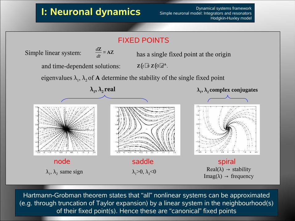
Hartmann-Grobman theorem states that “all” nonlinear systems can be approximated (e.g. through truncation of Taylor expansion) by a linear system in the neighbourhood(s)

of their fixed point(s). Hence these are “canonical” fixed points



Simple linear system:

eigenvalues λ1, λ2 of A determine the stability of the single fixed point

has a single fixed point at the origin

λ1, λ2 same sign λ1>0, λ2<0

λ1, λ2 real

node saddleReal(λ) → stability

Imag(λ) → frequency

λ1, λ2 complex conjugates

spiral

FIXED POINTS

AZZ =

dt

d

Z t( )= Z 0( )etA .and time-dependent solutions:

For example, the Van der Pol oscillator

Limit cycle attractor

Embedding manifold



,22

21 zzA += .arctan

1

2

= zzφ

… transformation of variables:


Z2 nullcline

Z1 nullcline

z2

NULLCLINES & MANIFOLDS

02 =z

( ) 01 122

1 =−− zzzµ

dz1

dt= z2 ,

dz2

dt= µ 1 − z1

2( )z2 − z1.

Unstable spiral

dV

dt= gNam∞ V( )× V − VNa( )+ gKn V( )× V − VK( )+ gL × V − VL( )+ I ,

Conductance based model of transmembrane voltage due

to ion channel currents

Slow potassium channel



m∞(V ) =mmax

1+ e Vm −V( ) σ ,n∞(V ) =nmax

1+ e Vn −V( ) σ ,

Sigmoid shaped channel activation

functions

-1 -0.8 -0.6 -0.4 -0.2 0 0.2 0.4 0.6 0.8 10

0.2

0.4

0.6

0.8

1

V

n

-8 -6 -4 -2 0 2 4 6 8 10

time (ms)

V1

n(V,t) n∞(V1)

n∞(V2)

V2V(t)

( ) ( )( )( )V

VnVn

dt

Vdn

nτ−= ∞)(

“instant” Na channel

dV




dn

dt=

n∞ − n( )τ n


-80 -60 -40 -20 0 20-0.1

0

0.1

0.2

0.3

0.4

0.5

0.6

n

V (mV)-80 -60 -40 -20 0 20

-0.1

0

0.1

0.2

0.3

0.4

0.5

0.6

n

V (mV)n nullcline

V nullcline Heteroclinic orbit

Stable focus Saddle Unstable spiral



m∞(V ) =mmax

1+ e Vm −V( ) σ ,n∞ (V ) =nmax

1+ e Vn −V( ) σ ,

2 4 6 8 10-80

-70

-60

-50

-40

-30

-20

-10

0

10

dV




“Low threshold” parameters (Izhikevich 2005)

-80 -60 -40 -20 0 20-0.1

0

0.1

0.2

0.3

0.4

0.5

0.6

time (ms)

V (mV)

V (mV)

n

suprathreshold

subthreshold



m∞(V ) =mmax

1+ e Vm −V( ) σ ,n∞ (V ) =nmax

1+ e Vn −V( ) σ ,dn

dt=

n∞ − n( )τ n


dV




dn

dt=

n∞ − n( )τ n




0 10 20 30 40 50-80

-70

-60

-50

-40

-30

-20

-10

0

10

-80 -60 -40 -20 0 20-0.1

0

0.1

0.2

0.3

0.4

0.5

0.6

0 10 20 30 40 50-80

-70

-60

-50

-40

-30

-20

-10

0

10

-80 -60 -40 -20 0 20-0.1

0

0.1

0.2

0.3

0.4

0.5

0.6

n

V (mV)

V

time (ms)

(d)(c)

n V

(b)(a)

m∞(V ) =mmax

1+ e Vm −V( ) σ ,n∞ (V ) =nmax

1+ e Vn −V( ) σ ,

Low threshold parameters

(Izhikevich 2005)

“saddle node” bifurcation

→ current “integrators”

Individual Neurons

Depending on the strength of synaptic currents, these neurons exhibit either by stochastic (left) or periodic/deterministic (right) firing rates

dV






,tan stochastictcons III += Noisy (Poisson) modulation of constant background rate

subthreshold + noise suprathreshold + noise

dV




dn

dt=

n∞ − n( )τ n




m∞(V ) =mmax

1+ e Vm −V( ) σ ,n∞ (V ) =nmax

1+ e Vn −V( ) σ ,

0 20 40 60 80 100 120-80

-70

-60

-50

-40

-30

-20

-10

0

n

V

time (ms)

-80 -60 -40 -20 0 20-0.1

0

0.1

0.2

0.3

0.4

0.5

0.6

0.7

0.8

0 20 40 60 80 100 120-80

-70

-60

-50

-40

-30

-20

-10

0

-80 -60 -40 -20 0 20-0.1

0

0.1

0.2

0.3

0.4

0.5

0.6

0.7

0.8

-80 -60 -40 -20 0 20-0.1

0

0.1

0.2

0.3

0.4

0.5

0.6

0.7

0.8

0 20 40 60 80 100 120-80

-70

-60

-50

-40

-30

-20

-10

0

n

V (mV)

V

time (ms)

n

V (mV)

V

time (ms)

V (mV)

High threshold parameters (Izhikevich

2005)

“Hopf” bifurcation

→ input “resonators”






CdV t( )

dt= g

Naf

NaV t( )( )× V t( )− V

Na( )+ gK

fK

V t( )( )× V t( )− VK( )

+gL

× V t( )− VL( )+ I ,

fNa (V ) = m(V )M h(V )H

fK (V ) = n(V )N

( ) ( )( )( )V

VmVm

dt

Vdm

mτ−= ∞)(

( ) ( )( )( )V

VhVh

dt

Vdh

mτ−= ∞)(

( ) ( )( )( )V

VnVn

dt

Vdn

nτ−= ∞)(

Fast sodium channel

sodium inactivation channel

-1 -0.5 0 0.5 1

0

0.2

0.4

0.6

0.8

1

h

V (mV)

m

n


Networks of ensemblesII: Ensembles of spiking neurons

1. Make a two-compartment neuron, with synaptic and dendritic compartments

HOW TO CONNECT NEURONS

( ) ( ) ,somaion

ionsomaionsoma IVVVf

dt

dVC +−×= ∑ Conductance based model of

cell soma compartment

( ) ..2 tett ααη −=

Post-synaptic currents

Synaptic and dendritic filtering 0 5 10 15 20 25 30

0

0.02

0.04

0.06

0.08

0.1

0.12

0.14

0.16

time (ms)

nu(t

)

1250 −= msα

1400 −= msα

( ) ( ) ( ).∑ −=m

msynapse

msoma TITttI η

Passive dendritic compartment

II: Ensembles of spiking neurons

Clouds and moments

( )( ) ,,H∑ ++−=j

sensorynoisejjjcsynapse IItxI τδ

Microscopic Ensemble

In this example, stimulus-induced currents induce a change from stochastic (time-space) activity to coherent periodic dynamics

Z2. Couple neurons together through synaptic currents

Synaptic currents in each individual

neuron Interneuron connectivity (H) and

efficacy (c)

Stochastic inputs (continuous Poisson

noise)

Afferent input from sensory neurons (on

or off)



Cell j firing event

Saddle node bifurcation

( )( ) ,,H∑ ++−=j

sensorynoisejjjcsynapse IItxI τδZ2. Couple neurons together through synaptic currents

Synaptic currents in each individual

neuron Interneuron connectivity (H) and

efficacy (c)

Stochastic inputs (continuous Poisson

noise)

Afferent input from sensory neurons (on

or off)



Cell j firing event


In this example, stimulus-induced currents induce a change from stochastic (time-space) activity to coherent periodic dynamics


When the stimulus is present, the deterministic dynamics cause a contraction in the ensemble density “cloud”.

Studying an entire ensemble of neurons allows one to visualise the evolution of the entire distribution of activity



e.g. Harrison et al. (2005), Deco et al. (2007) PLoS CB,

Breakspear et al. (2008) Brain Imaging and Behaviour

Ensemble density models

where p describes a neural ensemble density of states v(t), evolving according to deterministic f and stochastic D processes

( ) .. pDfp ∇−−∇=

f=“drift”

D=“diffusion”



Two ensemble network

First ensemble receives “sensory input”

Inter-network coupling modulated by an “attentional modulation”



Buchel, C., Friston, K.J., (1997) Cereb. Cortex. 7: 768–778.Friston KJ, Büchel C (2000) Proc. Natl. Acad. Sci. USA. 97, 7591-7596.

Mean synaptic current

Inter-spike variance

Inter-spike kurtosis



ENSEMBLE 1Stimulus onset Stimulus offset

Inter-spike interval (t)

Inte

r-sp

ike

inte

rval

(t-

1)





ENSEMBLE 1


ENSEMBLE 2


Inter-spike covariance

V i

Q i

( ) sensorynoiseiieeae IIf

dt

d ++= ςµςµµ,,,

VT0

1

µ

ς

Mean ensemble membrane potential ,

µ=<V>

Mean ensemble firing rate


Mean field oscillations: Spontaneous and inducedIII: Mesoscopic neural mass models

.26.0

,0.0

,015.0

3

2

1

−=Λ=Λ=Λ

Lyapunov spectra (tendency of orbits to diverge/converge)

III: Mesoscopic neural mass models

The centre of mass



( ) ( ),)1(.,,, iV

jV

iiiV

ii

QCQCGWZQVfdt

dV −++=

V j

Q jV i

Q i

C

Interactions between two neural subsystems modifying the evolution of the local pyramidal cells to,

Coupling parameter

V

Z

W

V2

V1



C=0

V

Z

W

V2

V1



C=0.16



λ

Λ1

Λ2

λ1

λ2

C

‘blowout’ bifurcation (Ott, Sommerer 1994)

-0.6 -0.4 -0.2 0 0.2 0.4-0.6

-0.4

-0.2

0

0.2

0.4

V1

V2

Λ1

λ1

V

Z

W

V2

V1



C=0.12



V

Z

W

Vi-Vj

W1-W2 time



P

G(Q)

Q

G-1(P)

G-1(P)

N

xi

xj

A

λ

Λ1

Λ2

λ1

λ2

C

λp

‘bubbling’ (Ashwin et al. 1994)

Monoaminergic neurons

V i

Q i

V i

Q iV i

Q i

V i

Q iV i

Q i

CC

A cortical array is constructed by coupling

an ensemble of subsystems

-30 -20 -10 0 10 20 300

0.2

0.4

0.6

0.8

1

.),( h

ji

KjiH

xx −=

h=1

h=0.1

h=0.01

h=4

The strength of the coupling drops inversely with

subsystem separation.

It may be 1-D or 2-D

Cortical clustering:

Relatively sparse excitatory connectivity between local modules (cortical columns), each consisting of densely interconnected excitatory

and inhibitory neurons

Image from Nunez 1997 (Neocortical Rhythms)



2-D Isotropic (symmetric) 1-D anisotropic

II: Ensembles of spiking neurons From ensembles to mean fieldsA local mean field oscillator


Narrow footprint: Local synaptic inputsBroad synaptic

footprint: No input





Real brain tractography

centrality

Anatomical connectivity matrix

( ) Ifdt

diieea

e += ςµςµµ,,,

Spontaneous cortical activity

Functional connectivity matrix

Honey, Kotter, Breakspear, Sporns (2007) PNAS

( ) ( ) ττµτ

dttHRFtS e∫ −= )(

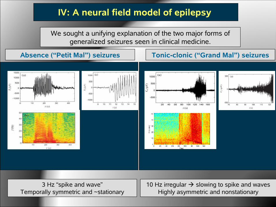
IV: A neural field model of epilepsy

Primary generalized seizures are those which arise almost simultaneously across the entire cortex.

IV: A “neural field” model of epilepsy


Absence (“Petit Mal”) seizures Tonic-clonic (“Grand Mal”) seizures

We sought a unifying explanation of the two major forms of generalized seizures seen in clinical medicine.

3 Hz “spike and wave”Temporally symmetric and ~stationary

10 Hz irregular slowing to spike and wavesHighly asymmetric and nonstationary


Va membrane potentials

Φa field potentials

Qa firing rates

a=e,i cortical populations

a=s specific thalamic n.

a=r reticular thalamic n.

To do so, we employed a neural “mean field” approach,

where D is a (spatiotemporal) differential operator acting on V, a vector of neural states

which vary continuously across a smooth cortical

sheet.

( ) ( )),(,. tFtD xVxV a=

Each of the entries of V, represents the mean value of a neural state in a

local populations (~cm2).


Robinson et al. (2002) Phys Rev. E 65:041924.

Corticothalamic connectivity

where

describes dendritic filtering of synaptic currents

),2,(),(),(),( 0ttvtvtvtVD sasiaieaea −++= rrrr φφφα

1111

2

2

+∂∂

++∂∂=

ttD

βααβα

),,(),(),()2,(),( 0 tvtvtvttvtVD nanrarsaseaea rrrrr φφφφα +++−=

8 9 10 11 12 13

11.76

11.78

11.8

11.82

11.84

11.86

model

time (sec)

Φe

79 80 81 82 83

-100

-50

0

50

100

EEG

time (sec)

Pz

Va membrane potentials

Φa field potentials

Qa firing rates

Cortico-cortical connectivty

where

describes propagating cortical field potentials

Jirsa & Haken (1996) PRL

.21 222

2

2

2

∇−+

∂∂+

∂∂= aaa

aa v

ttD γγ

γ

( ) [ ],),(, tVStD aaa rr =φ

a=e,i cortical populations

a=s specific thalamic n.

a=r reticular thalamic n.

0 2 4 6 8 10 126

8

10

12

14

time (sec)

Φe

strongly damped


μse μse

Φe

(s-1)

Φe

(s-1)

3 Hz instability

μse

Φe

(s-1)

10 Hz instability

μse

Φe

(s-1)

Breakspear et al. (2006) Cerebral Cortex doi:10.1093/cercor/bhj072

Global mode instabilities

1. Ignore spatial derivatives ( ) & 2. explore nonlinear bifurcations by changing μse 02 =∇

model Cortex-reticular–specific loop

data

model Cortex-specific loop

data

Discussion

Deco et al. (2007) PLoS CB, Breakspear et al. (2008) Brain Imaging and Behaviour

I : Cortical field models

where

describes propagating cortical field potentials in cortical, thalamic and reticular populations

.21 222

2

2

2

∇−+

∂∂+

∂∂= aaa

aa v

ttD γγ

γ

( ) [ ],),(, tVStD aaa rr =φ

8 9 10 11 12 13

11.76

11.78

11.8

11.82

11.84

11.86

model

time (sec)

Φe

79 80 81 82 83

-100

-50

0

50

100

EEG

time (sec)

Pz

II: Ensemble density models

where p describes a neural ensemble density of states v(t), evolving according to deterministic f and stochastic D processes

( ) ( )..

∂∂

∂∂+

∂∂−=∇−−∇=

v

pD

vv

fptrpDfp

III: Neural mass models

describes local cortical ensembles (j) interacting through induced synaptic currents, with distant ensembles (k) in the presence of

noise.

( ) ( ) .,,, , σςςµςµµIgHf

dt

d

k

keckj

je

je

je

jea

je ++= ∑

Breakspear, Stam, Williams (2003) JCNS

Honey, Kotter, Breakspear, Sporns (2007) PNAS

Jirsa & Haken (1996) PRL, Robinson (2002) PRE, Breakspear et al. (2006) Cerebral Cortex

Probabilistic inference

Self organization

and complexity

Detailed biophysical

validity

?Cortical Statistics?

Discussion

Hence we require a model that allows multistability and non-Gaussian statistics at all scales

Freyer, Aquino, Robinson, Ritter, Breakspear (2009). Journal of Neuroscience

Acknowledgements

Local Team Members

Stuart Knock, Kevin Aquino, Angela Langdon, Mika Rubinov, Mark Schira, Stewart Heitmann, Tjeerd Boonstra, Muhsin Karim, Norman Ferns,

Tamara Powell, Nicky Kochan

Funding Sources

James S. McDonnell Foundation (Brain NRG)ARC “Thinking Systems” Special Initiative

Further Reading

Izhikevich E (2005) Dynamical systems in neuroscience: The geometry of excitability and bursting. MIT Press.Jirsa, V., McIntosh, A.R. (2007) Handbook of Brain Connectivity. Springer.

Deco, G., Jirsa, V.K., Robinson, P.A., Breakspear, M., Friston, K.J. (2007) PLoS CB. (in press).Breakspear, M., Knock, S. (2008) Kinetic models of brain activity. Brain Imaging and Behaviour (in press).

computational models of the brain (michael breakspear)

Documents