computational ⊗⊘ photography - computer graphics at...
TRANSCRIPT

⊕⊖ Computational ⊗⊘ Photography
Image Stabilization
Jongmin Baek
CS 478 LectureMar 7, 2012
Wednesday, March 7, 12
Overview• Optical Stabilization
• Lens-Shift
• Sensor-Shift
• Digital Stabilization
• Image Priors
• Non-Blind Deconvolution
• Blind Deconvolution
Wednesday, March 7, 12

Blurs in Photography
Wednesday, March 7, 12
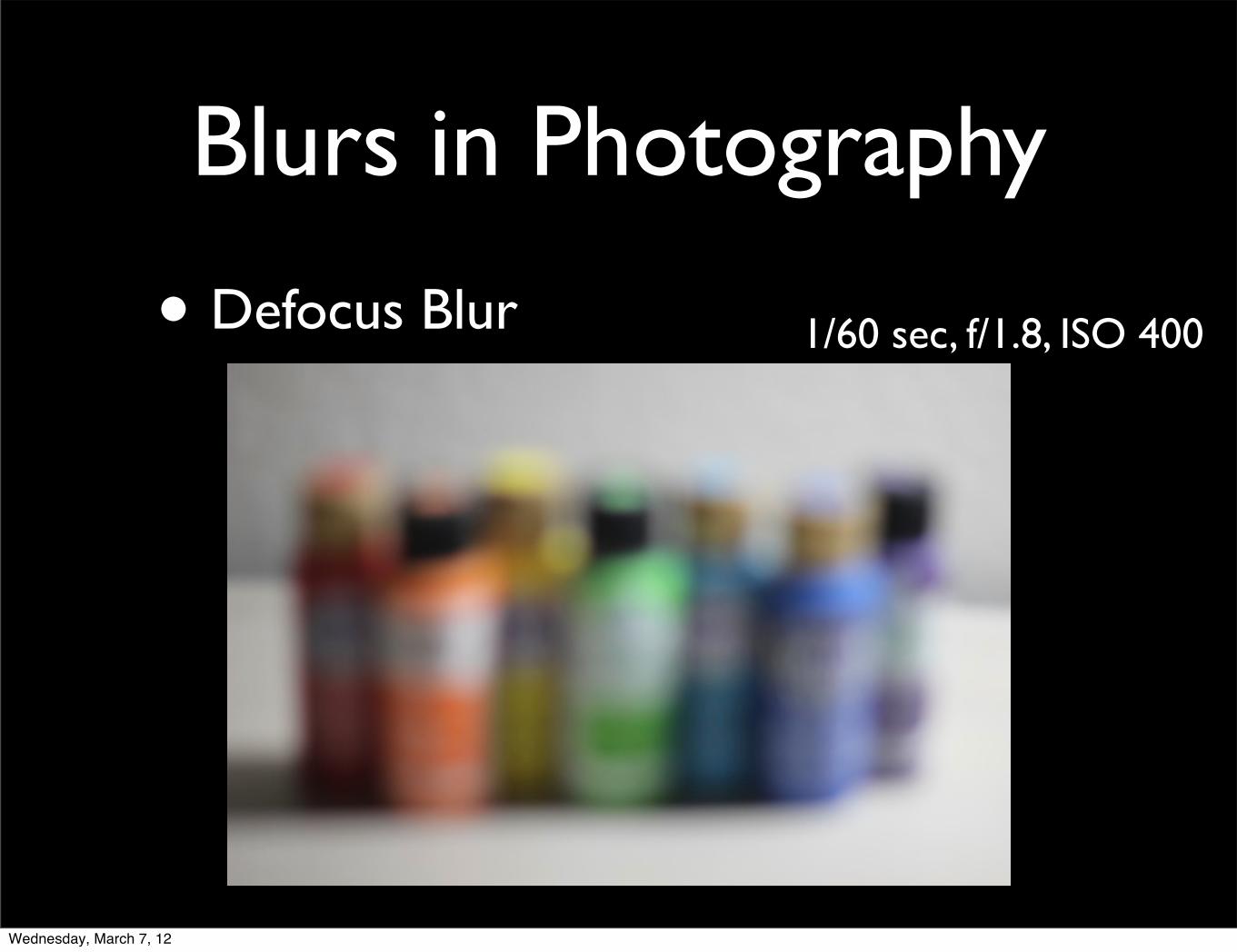
Blurs in Photography
• Defocus Blur 1/60 sec, f/1.8, ISO 400
Wednesday, March 7, 12
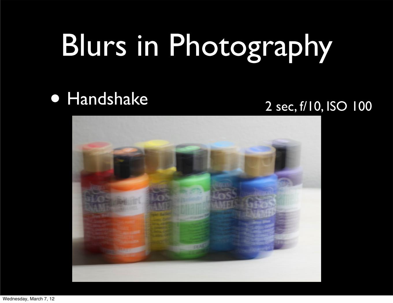
Blurs in Photography
• Handshake 2 sec, f/10, ISO 100
Wednesday, March 7, 12
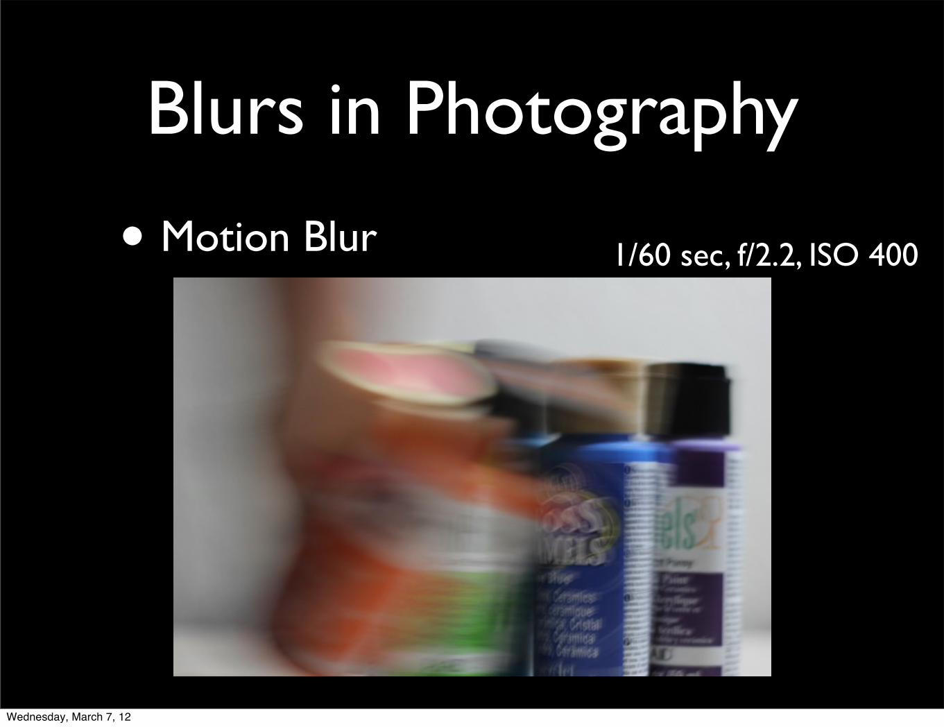
Blurs in Photography
• Motion Blur 1/60 sec, f/2.2, ISO 400
Wednesday, March 7, 12

Blurs in Photography
• Some blurs are intentional.
• Defocus blur: Direct viewer’s attention. Convey scale.
• Motion blur: Instill a sense of action.
• Handshake: Advertise how unsteady your hand is.
• Granted, jerky camera movement is sometimes used to convey a sense of hecticness in movies.
Wednesday, March 7, 12
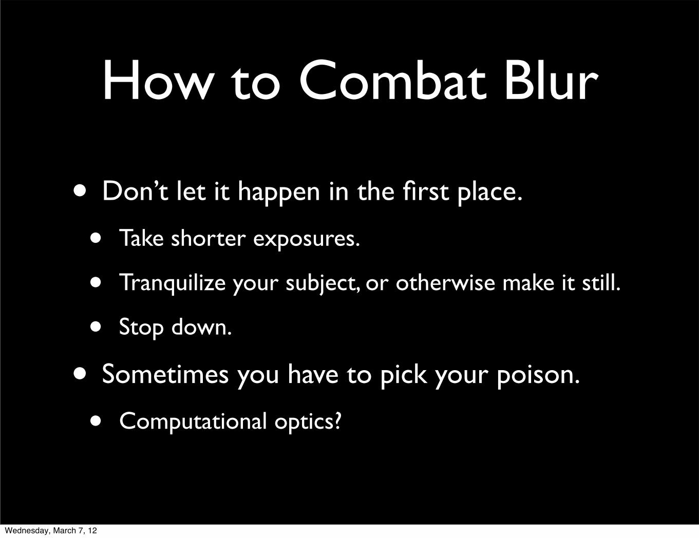
How to Combat Blur
• Don’t let it happen in the first place.
• Take shorter exposures.
• Tranquilize your subject, or otherwise make it still.
• Stop down.
• Sometimes you have to pick your poison.
• Computational optics?
Wednesday, March 7, 12
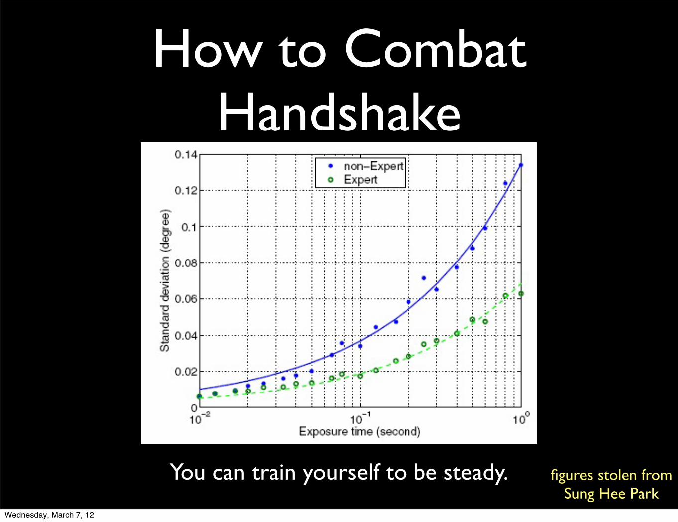
How to Combat Handshake
You can train yourself to be steady. figures stolen from Sung Hee Park
Wednesday, March 7, 12

How to Combat Handshake
Use a heavier camera. figures stolen from Sung Hee Park
Wednesday, March 7, 12
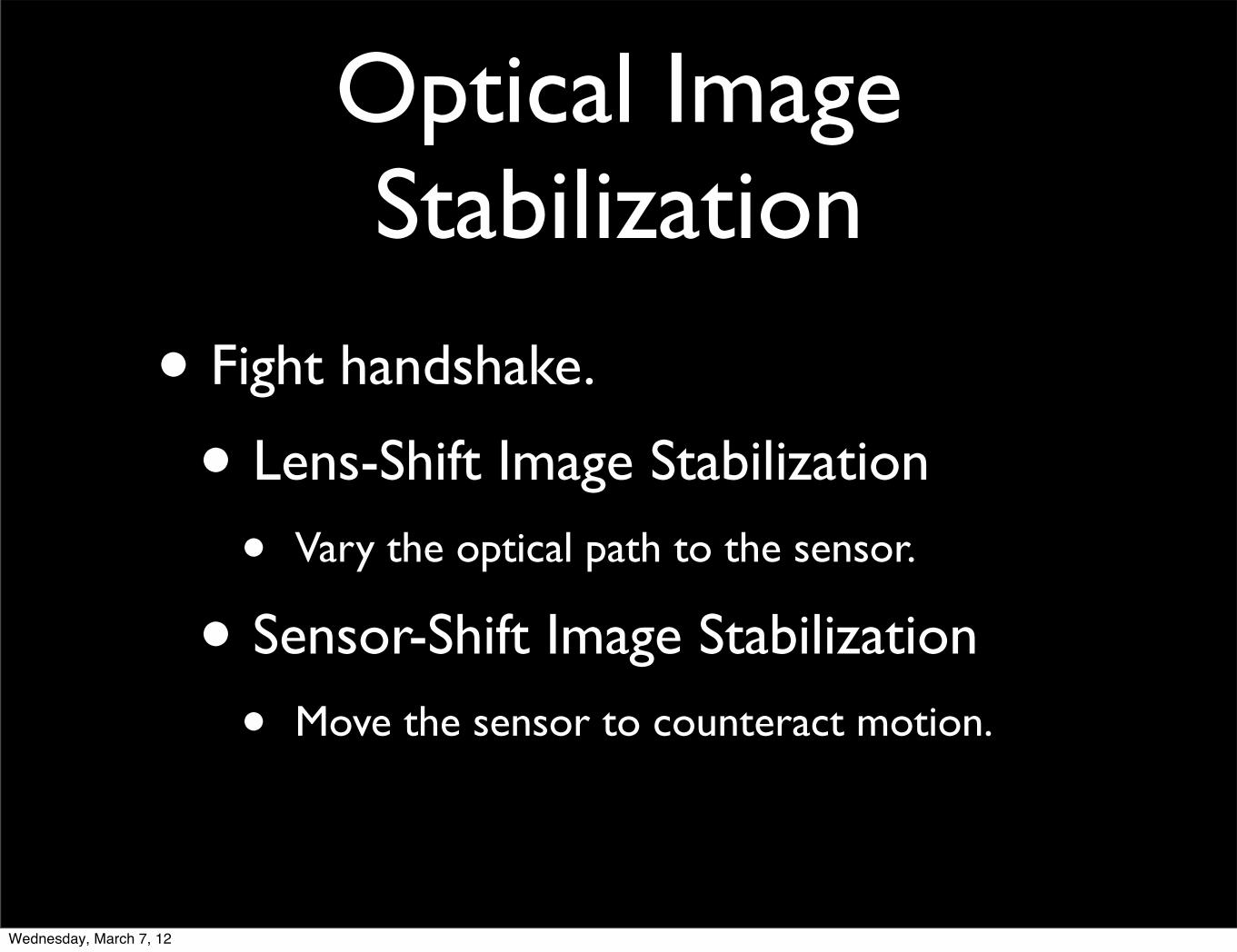
Optical Image Stabilization
• Fight handshake.
• Lens-Shift Image Stabilization
• Vary the optical path to the sensor.
• Sensor-Shift Image Stabilization
• Move the sensor to counteract motion.
Wednesday, March 7, 12
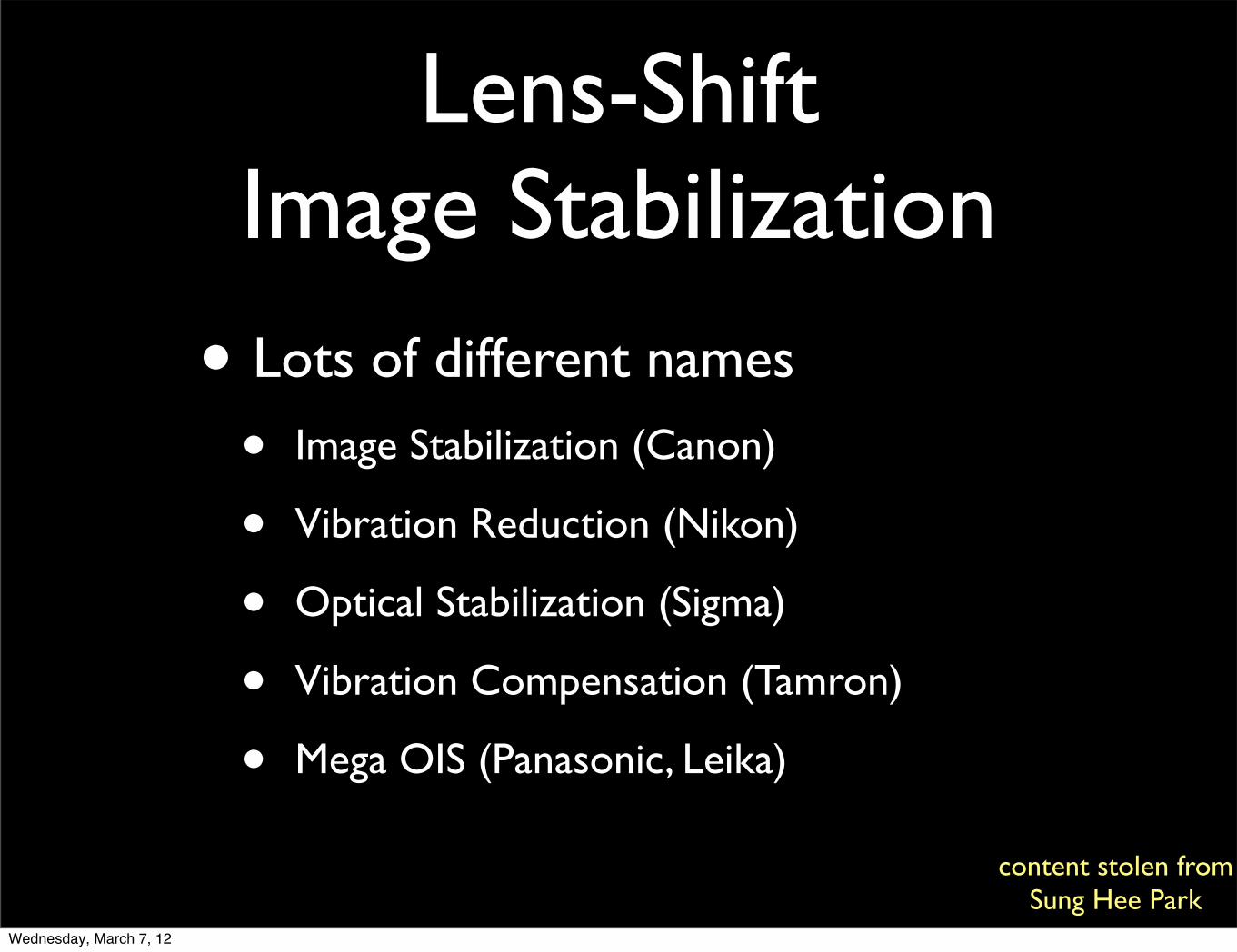
Lens-ShiftImage Stabilization
• Lots of different names
• Image Stabilization (Canon)
• Vibration Reduction (Nikon)
• Optical Stabilization (Sigma)
• Vibration Compensation (Tamron)
• Mega OIS (Panasonic, Leika)
content stolen from Sung Hee Park
Wednesday, March 7, 12

History of Image Stabilization
Year Lens Stability Characteristic1995 75-300mm f/4-5.6 IS USM 2 stop The first IS lens
1997 300mm f/4L IS USM 2 stops New IS mode
1999 300mm f/2.8L IS USM 2 stops Tripod detection
2001 70-200mm f/2.8L IS USM 3 stops
2006 70-200mm f/4L IS USM 4 stops
2008 200mm f/2L IS USM 5 stops
Canon IS
content stolen from Sung Hee Park
Wednesday, March 7, 12
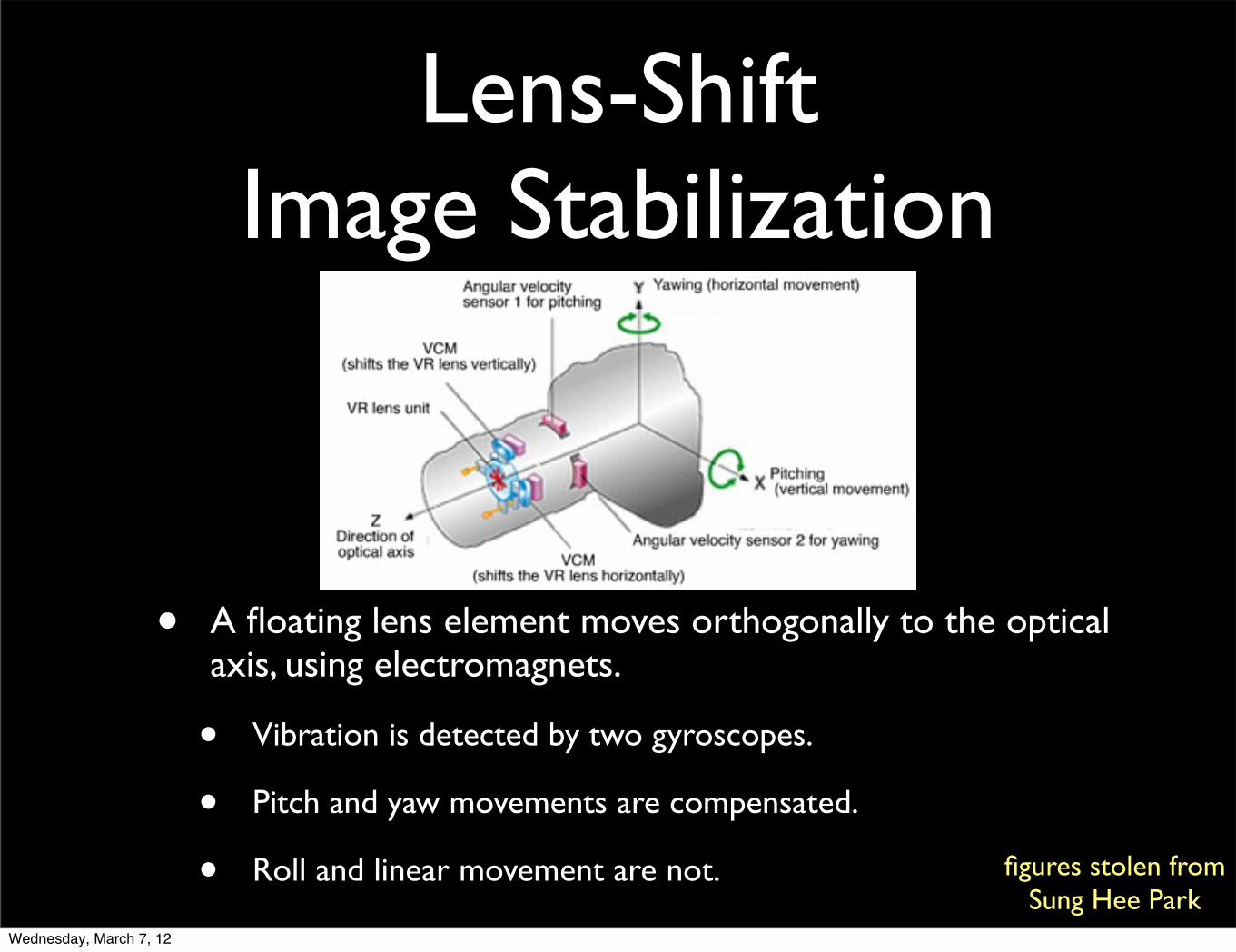
Lens-ShiftImage Stabilization
• A floating lens element moves orthogonally to the optical axis, using electromagnets.
• Vibration is detected by two gyroscopes.
• Pitch and yaw movements are compensated.
• Roll and linear movement are not. figures stolen from Sung Hee Park
Wednesday, March 7, 12
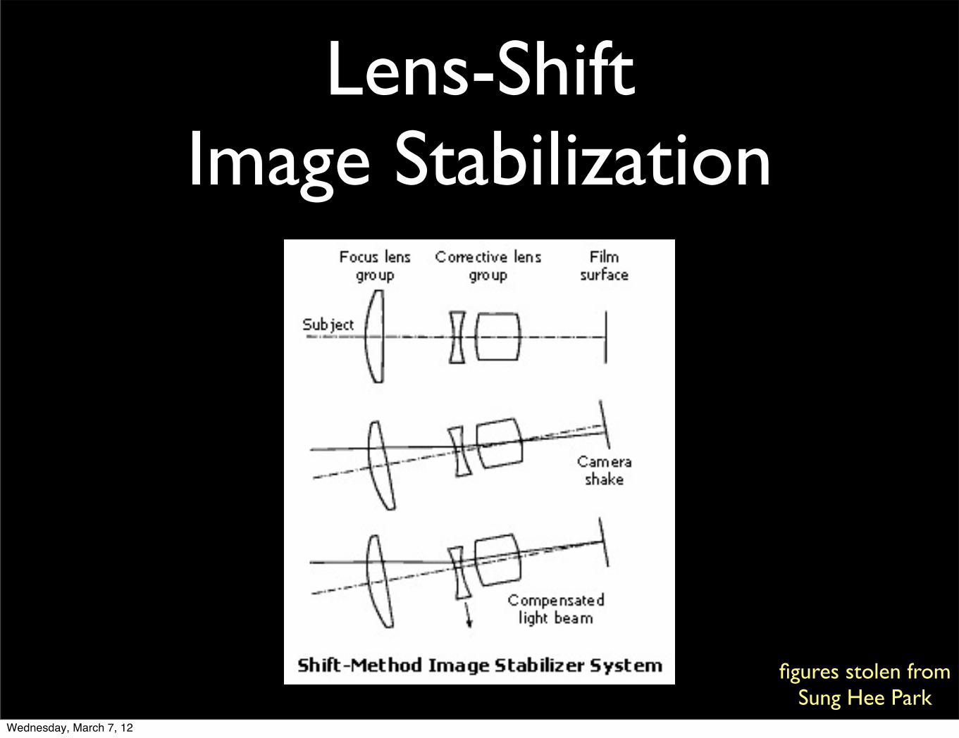
Lens-ShiftImage Stabilization
figures stolen from Sung Hee Park
Wednesday, March 7, 12
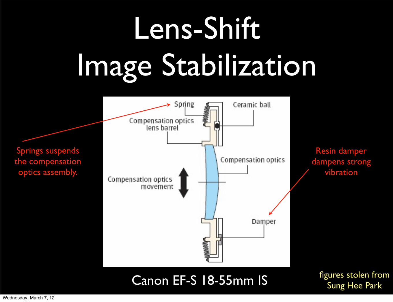
Lens-ShiftImage Stabilization
figures stolen from Sung Hee ParkCanon EF-S 18-55mm IS
Springs suspends the compensation optics assembly.
Resin damper dampens strong
vibration
Wednesday, March 7, 12
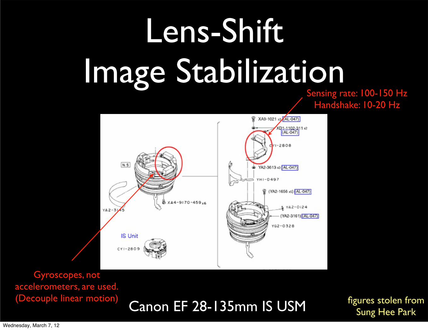
Lens-ShiftImage Stabilization
figures stolen from Sung Hee ParkCanon EF 28-135mm IS USM
Gyroscopes, not accelerometers, are used.(Decouple linear motion)
Sensing rate: 100-150 HzHandshake: 10-20 Hz
Wednesday, March 7, 12
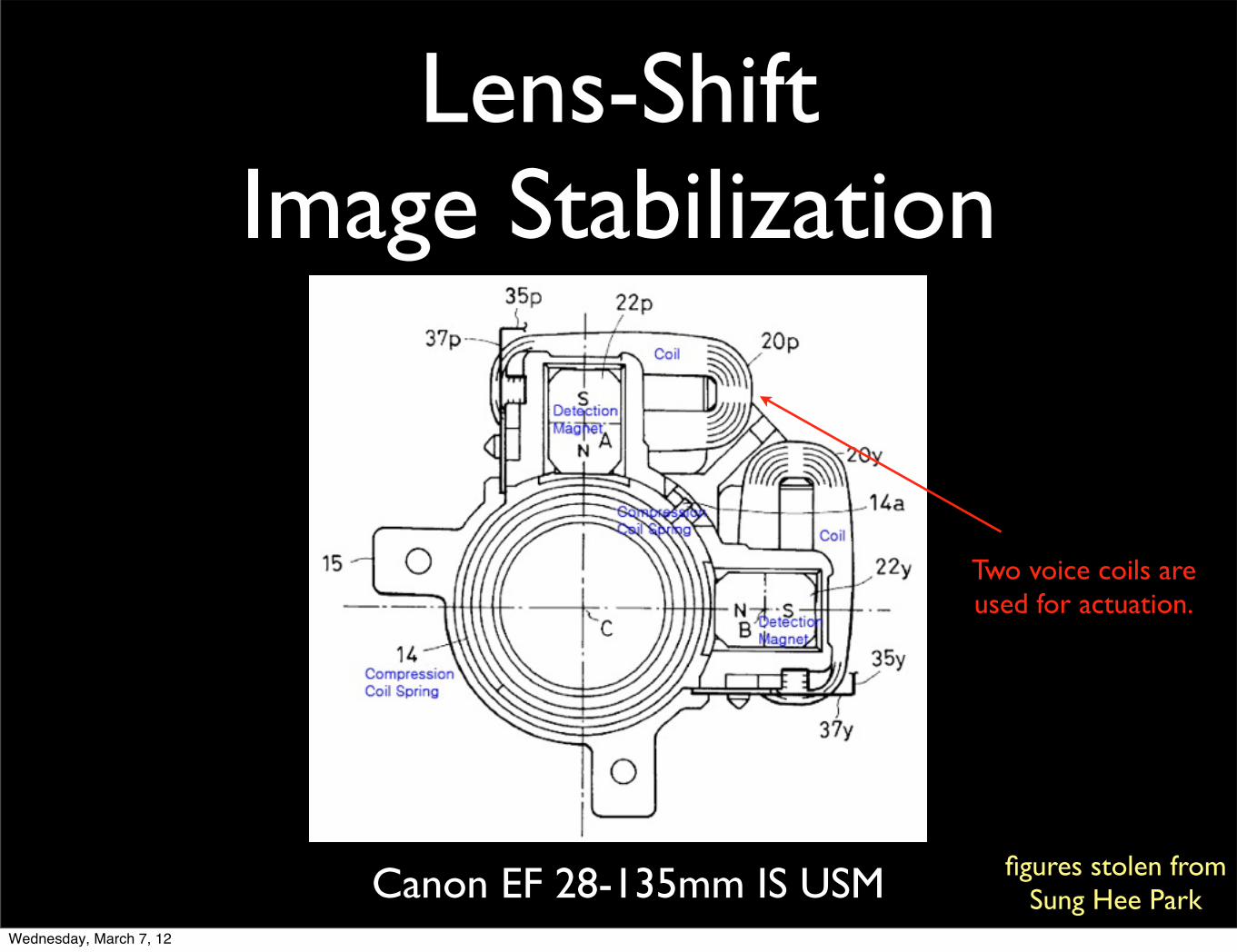
Lens-ShiftImage Stabilization
figures stolen from Sung Hee ParkCanon EF 28-135mm IS USM
Two voice coils are used for actuation.
Wednesday, March 7, 12

Lens-ShiftImage Stabilization
figures stolen from Sung Hee ParkCanon EF 28-135mm IS USM
Hall Sensors: varies output voltage in
response to change in magnetic field(feedback into
control system)
Wednesday, March 7, 12
Lens-ShiftImage Stabilization
• Video
• http://www.dpreview.com/reviews/konicaminoltaa2/Images/asmovie.mov
Wednesday, March 7, 12
Sensor-ShiftImage Stabilization
• Lots of different names, again
• Anti Shake (Minolta)
• Super Steady Shot (Sony)
• Shake Reduction (Pentax)
• Image Stabilization (Olympus)
content stolen from Sung Hee Park
Wednesday, March 7, 12
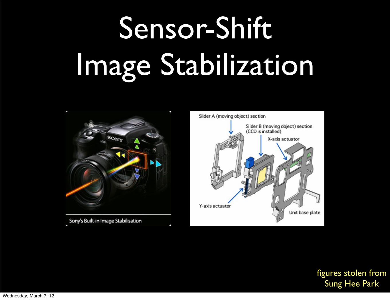
Sensor-ShiftImage Stabilization
figures stolen from Sung Hee Park
Wednesday, March 7, 12
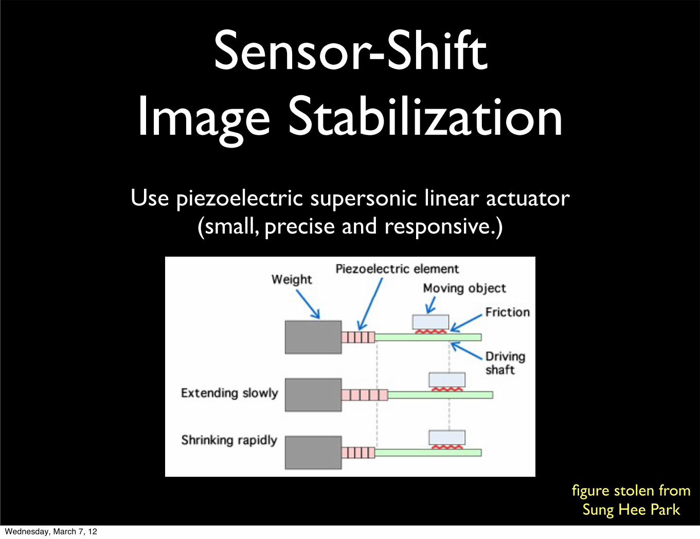
Sensor-ShiftImage Stabilization
figure stolen from Sung Hee Park
Use piezoelectric supersonic linear actuator (small, precise and responsive.)
Wednesday, March 7, 12
Sensor-ShiftImage Stabilization
• Video
• http://gizmodo.com/optical-image-stabilizer
Wednesday, March 7, 12
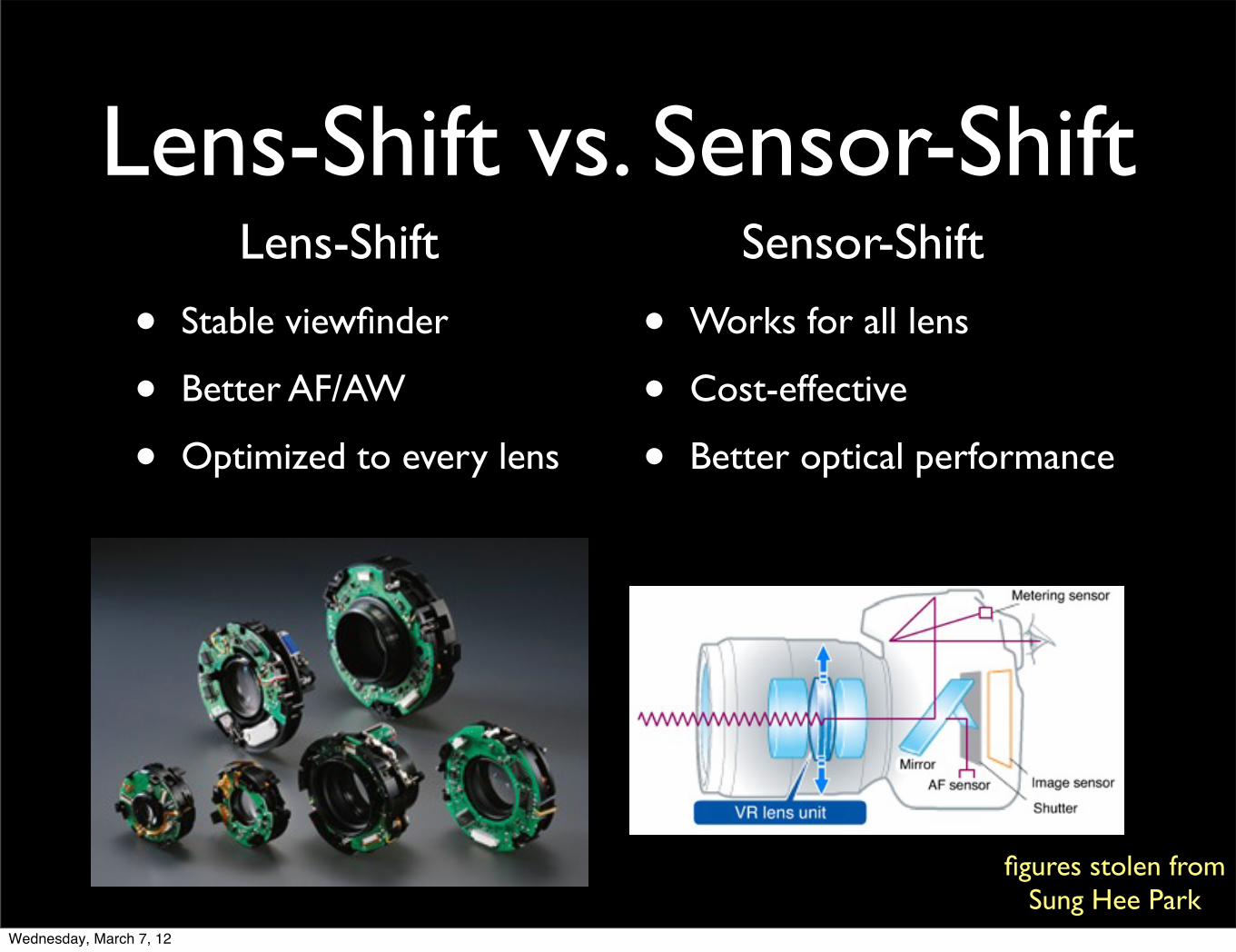
Lens-Shift vs. Sensor-Shift
figures stolen from Sung Hee Park
• Stable viewfinder
• Better AF/AW
• Optimized to every lens
• Works for all lens
• Cost-effective
• Better optical performance
Lens-Shift Sensor-Shift
Wednesday, March 7, 12
Digital Stabilization
• What if you already incurred blur?
• Need to “remove” blur
Wednesday, March 7, 12

Image Formation
• I = L ⊗ K + N
• I : Observation
• L : Latent image
• K : Blur kernel
• N : Noise
L K N
I
Wednesday, March 7, 12

Image Formation+Spatially varying blur
• I = ∑i( L ⊗ Ki .∗ Mi) + N
• I : Observation
• L : Latent image
• Ki : (Many) Blur kernels
• Mi : Influence map, ∑i Mi = 1
• N : Noise
Will only discuss spatially-invariant blur for now.Wednesday, March 7, 12
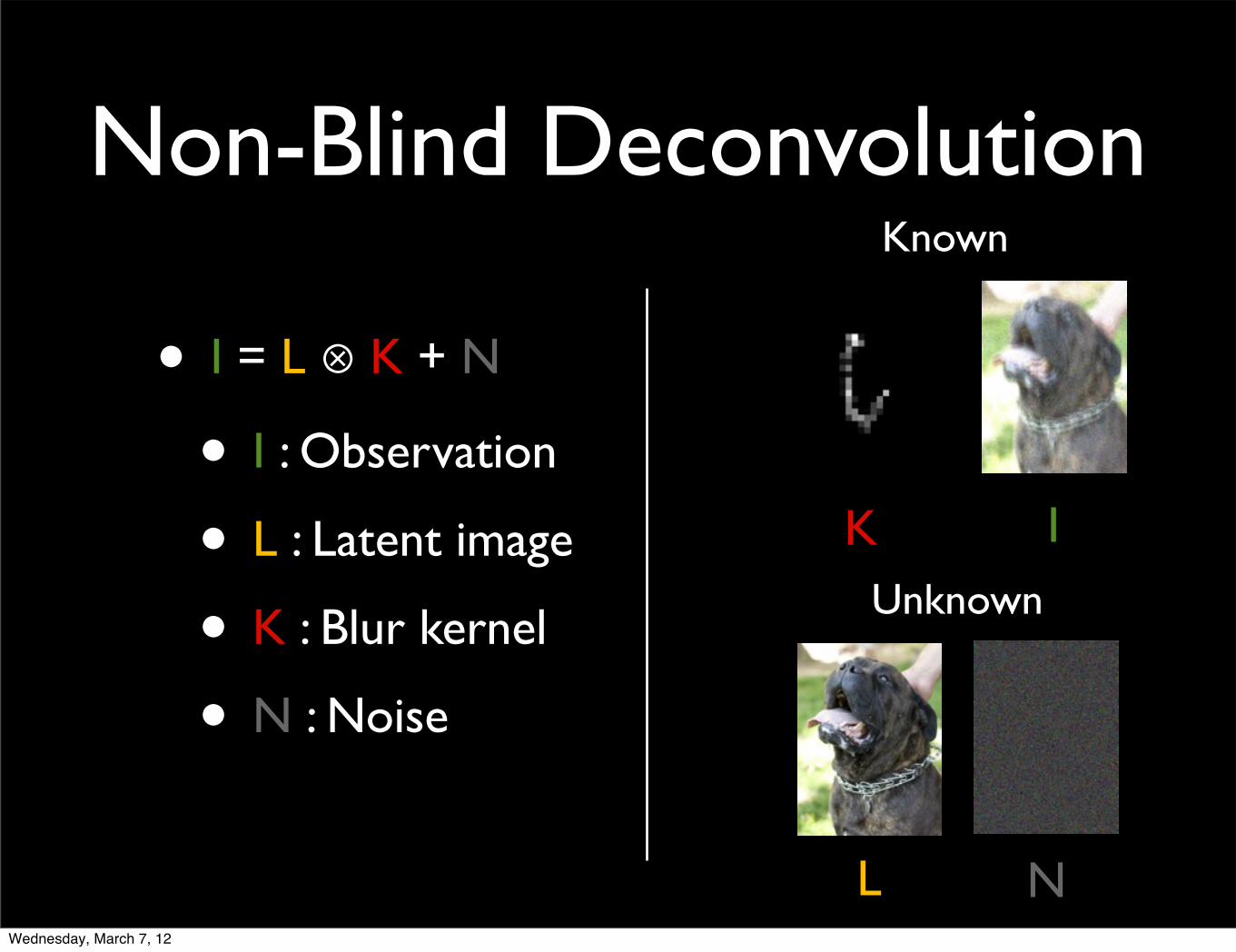
Non-Blind Deconvolution
• I = L ⊗ K + N
• I : Observation
• L : Latent image
• K : Blur kernel
• N : Noise
L N
Unknown
K I
Known
Wednesday, March 7, 12
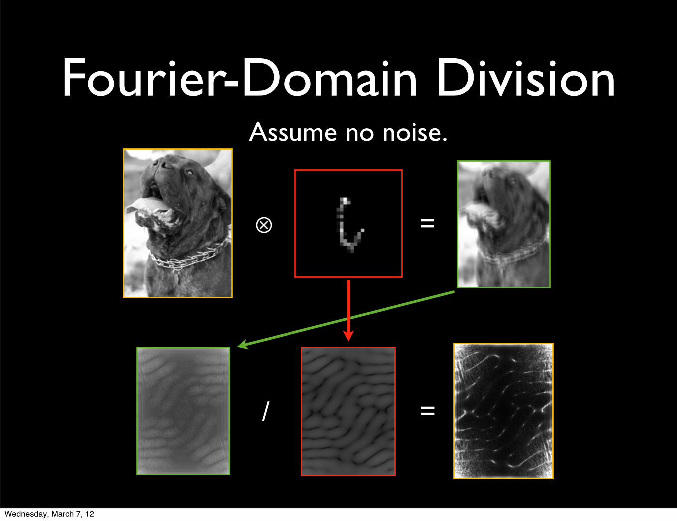
Fourier-Domain Division
⊗ =
=/
Assume no noise.
Wednesday, March 7, 12

Fourier-Domain Division
⊗ =
=/
Assume no noise.
What went wrong?Wednesday, March 7, 12
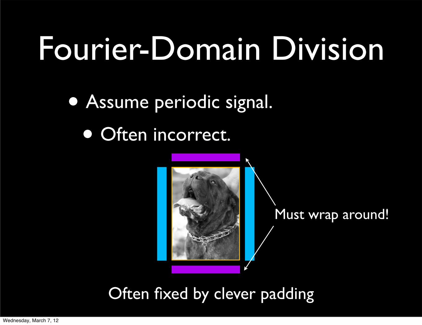
• Assume periodic signal.
• Often incorrect.
Fourier-Domain Division
Must wrap around!
Often fixed by clever paddingWednesday, March 7, 12
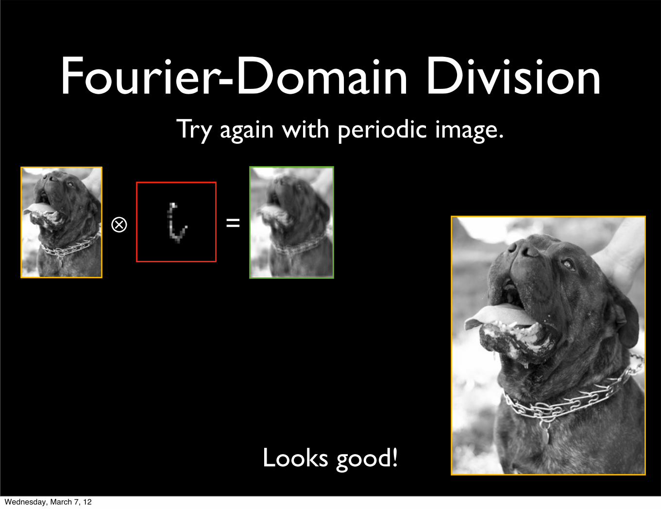
Fourier-Domain DivisionTry again with periodic image.
⊗ =
Looks good!Wednesday, March 7, 12
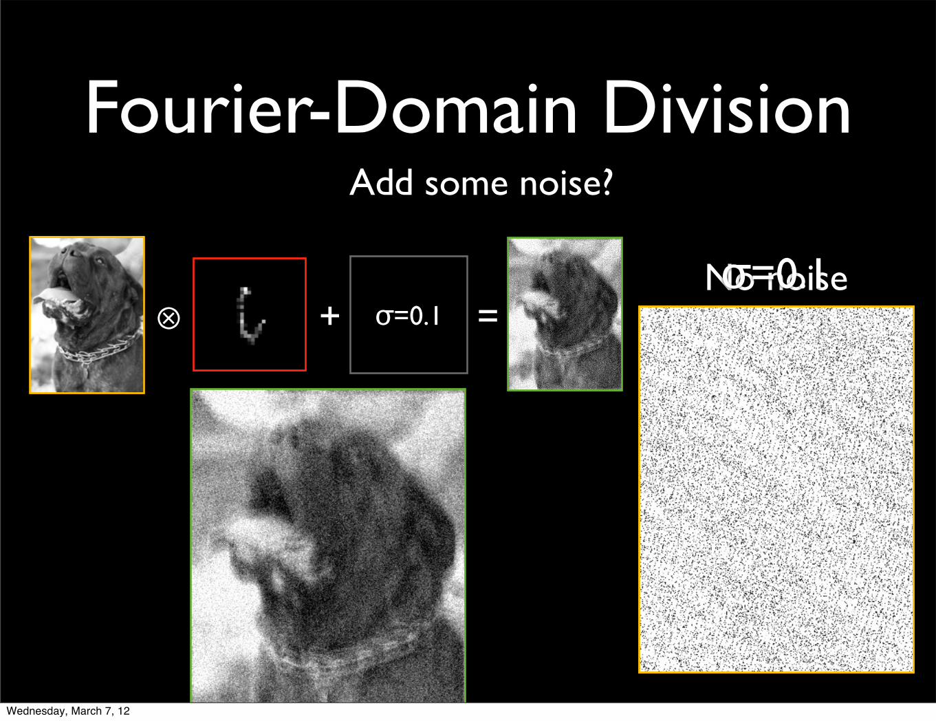
Fourier-Domain DivisionAdd some noise?
σ=0.1 =⊗ +No noiseσ=0.1
Wednesday, March 7, 12
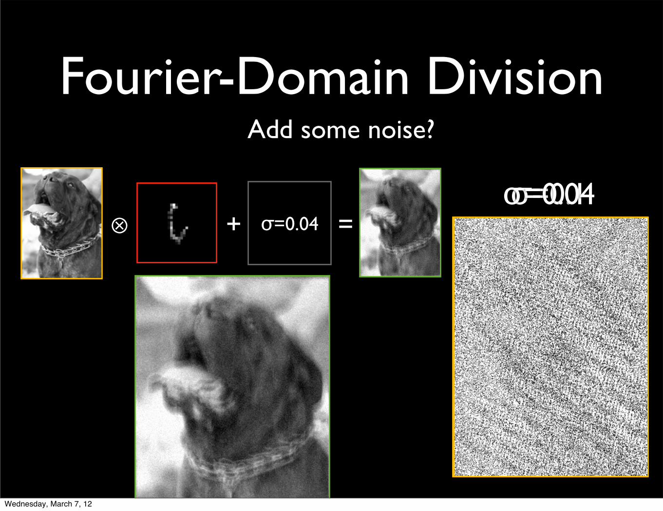
Fourier-Domain DivisionAdd some noise?
σ=0.04 =⊗ +σ=0.1σ=0.04
Wednesday, March 7, 12

σ=0.04σ=0.01
Fourier-Domain DivisionAdd some noise?
σ=0.01 =⊗ +
Wednesday, March 7, 12
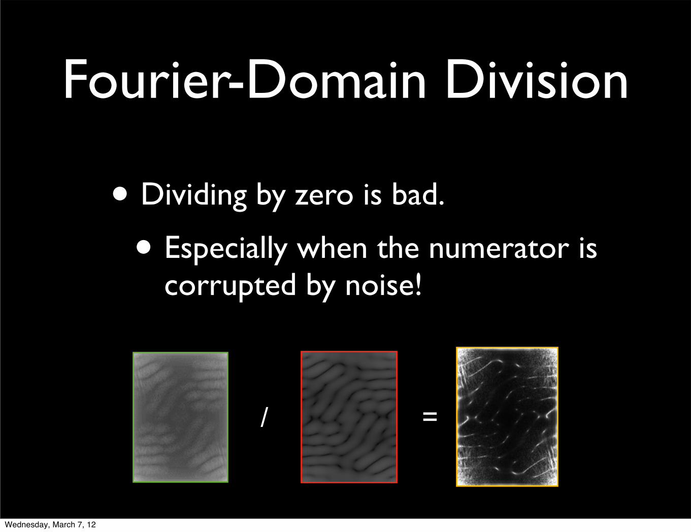
• Dividing by zero is bad.
• Especially when the numerator is corrupted by noise!
Fourier-Domain Division
=/
Wednesday, March 7, 12
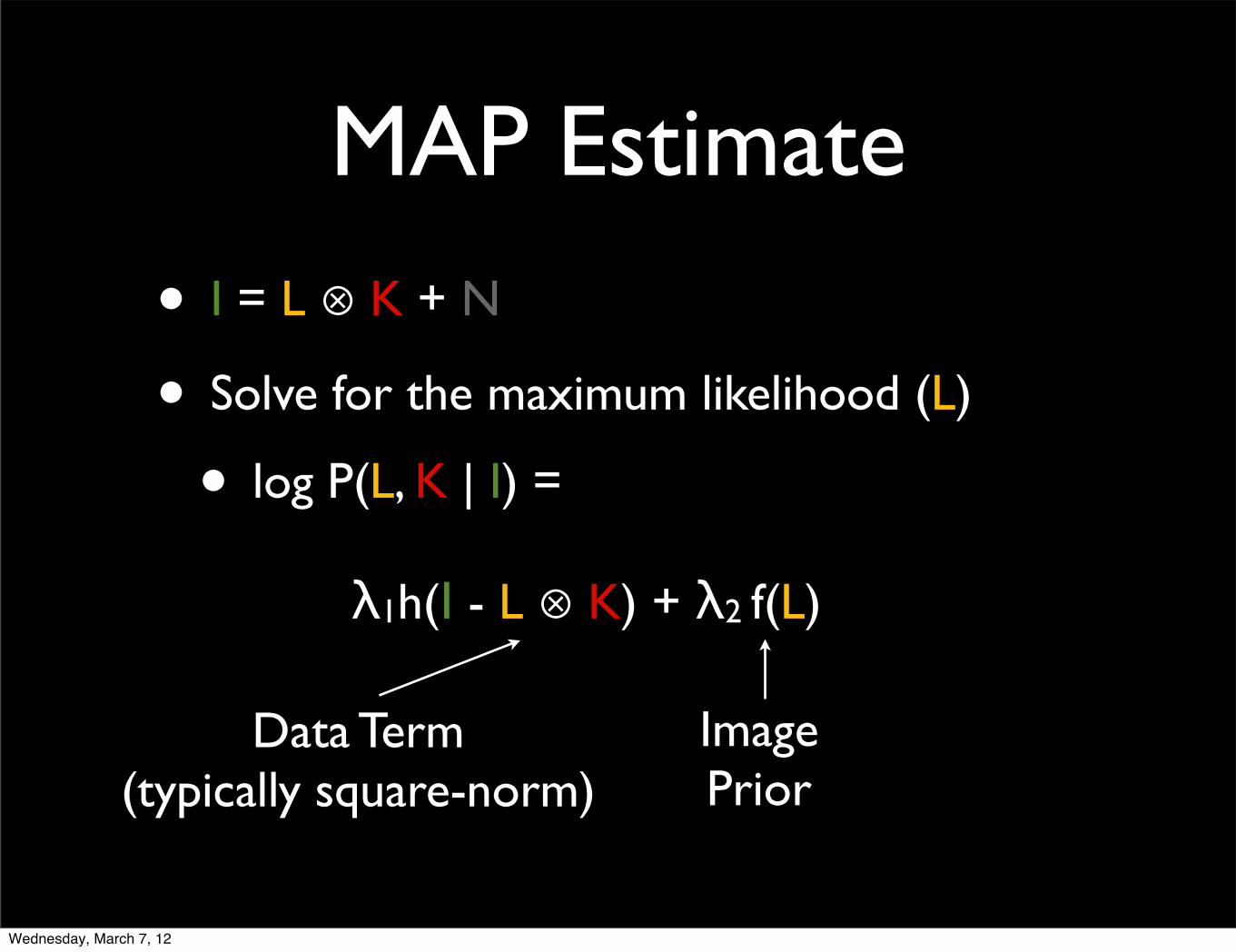
MAP Estimate
• I = L ⊗ K + N
• Solve for the maximum likelihood (L)
• log P(L, K | I) =
λ1h(I - L ⊗ K) + λ2 f(L)
Data Term(typically square-norm)
ImagePrior
Wednesday, March 7, 12
Image Priors
• f(L): should be high for natural images, and low for others.
• Often based on sparsity of gradients.
Wednesday, March 7, 12
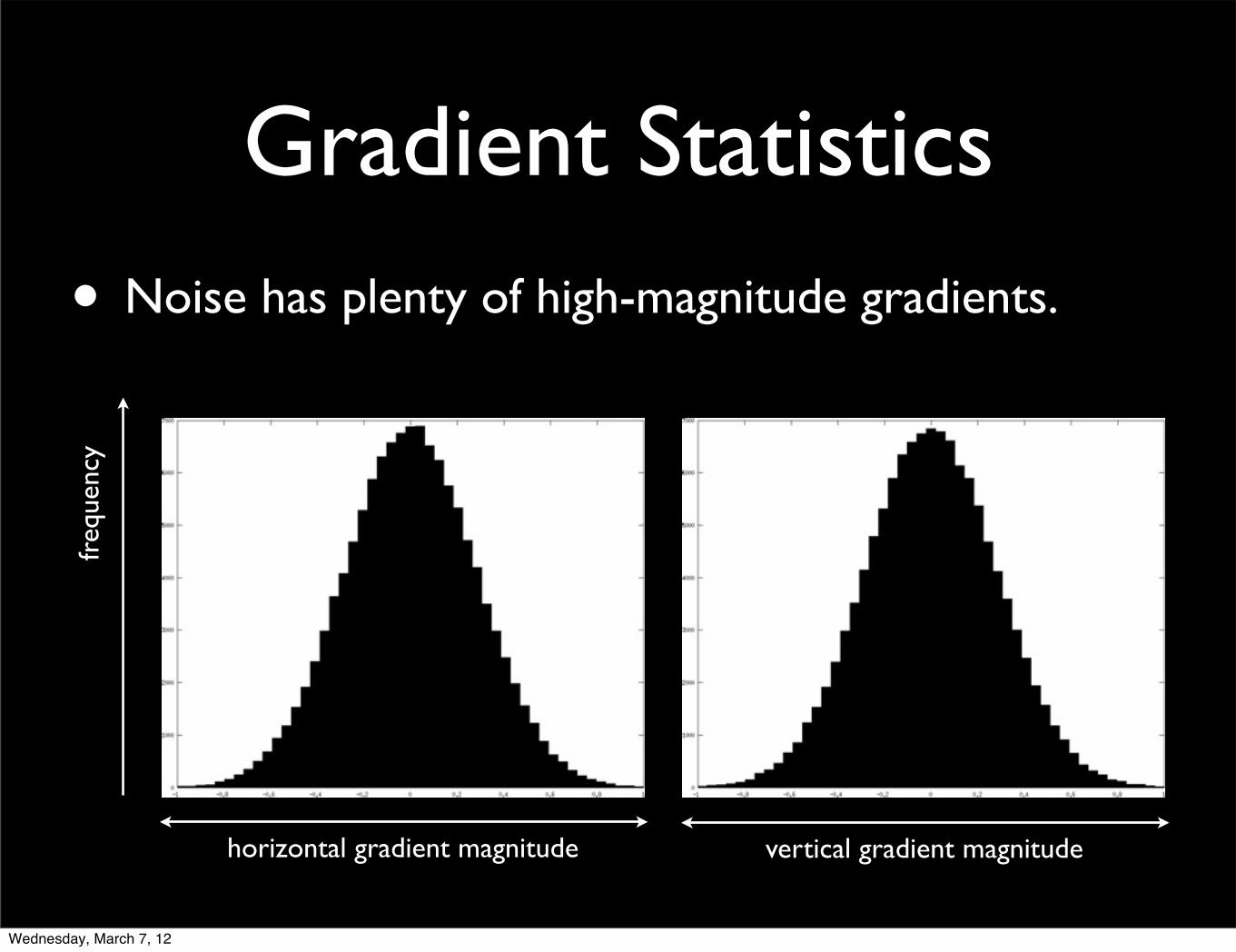
Gradient Statistics
• Noise has plenty of high-magnitude gradients.
freq
uenc
y
horizontal gradient magnitude vertical gradient magnitude
Wednesday, March 7, 12
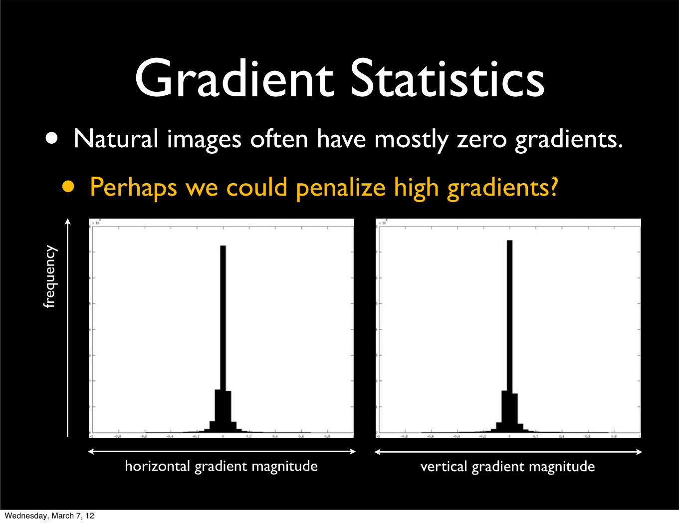
• Natural images often have mostly zero gradients.
• Perhaps we could penalize high gradients?
Gradient Statisticsfr
eque
ncy
horizontal gradient magnitude vertical gradient magnitude
Wednesday, March 7, 12
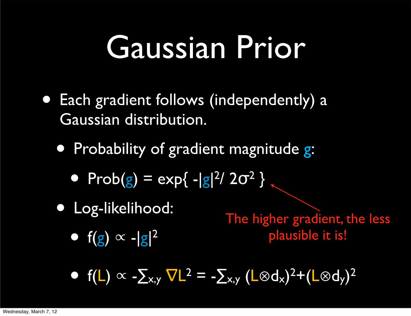
Gaussian Prior
• Each gradient follows (independently) a Gaussian distribution.
• Probability of gradient magnitude g:
• Prob(g) = exp{ -|g|2/ 2σ2 }
• Log-likelihood:
• f(g) ∝ -|g|2
• f(L) ∝ -∑x,y ∇L2 = -∑x,y (L⊗dx)2+(L⊗dy)2
The higher gradient, the less plausible it is!
Wednesday, March 7, 12
Gaussian Prior
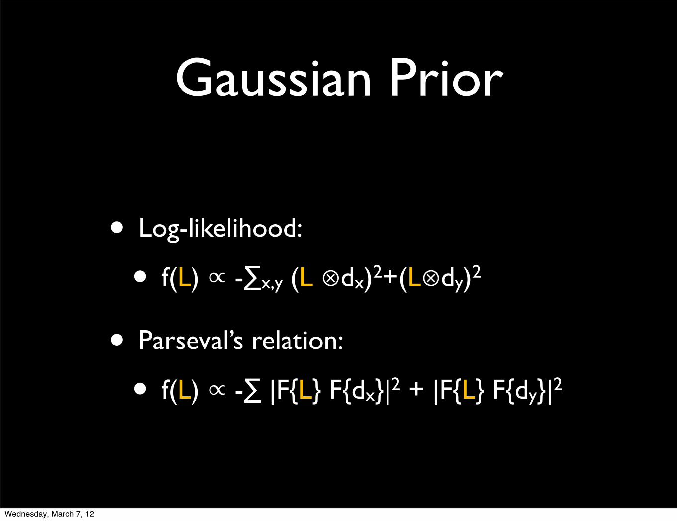
• Log-likelihood:
• f(L) ∝ -∑x,y (L ⊗dx)2+(L⊗dy)2
• Parseval’s relation:
• f(L) ∝ -∑ |F{L} F{dx}|2 + |F{L} F{dy}|2
Wednesday, March 7, 12
Gaussian Prior
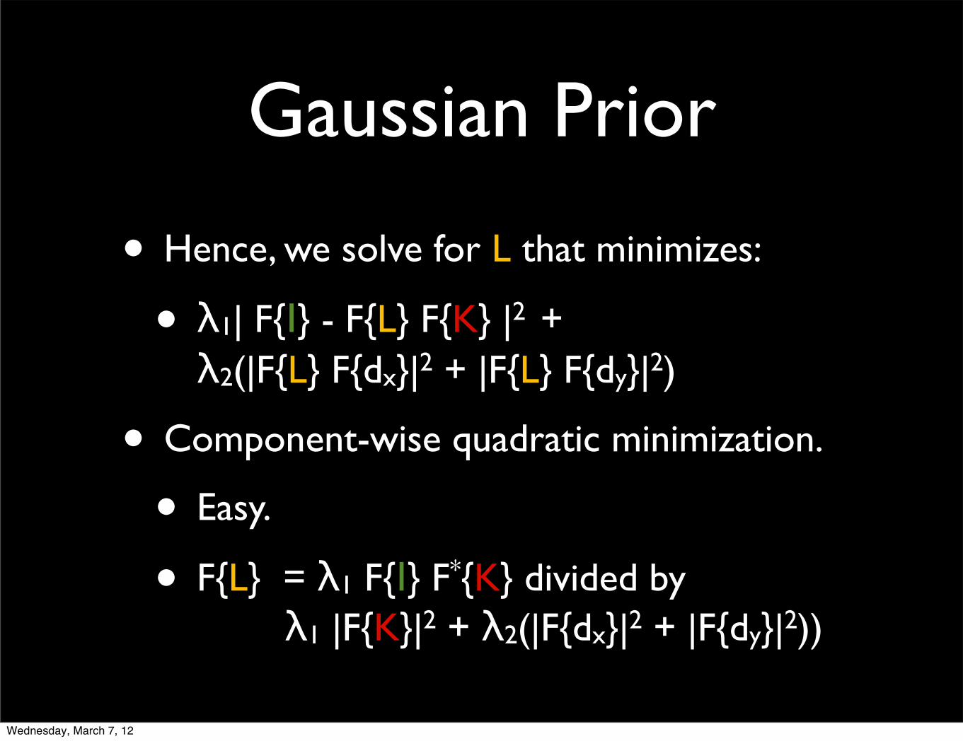
• Hence, we solve for L that minimizes:
• λ1| F{I} - F{L} F{K} |2 +λ2(|F{L} F{dx}|2 + |F{L} F{dy}|2)
• Component-wise quadratic minimization.
• Easy.
• F{L} = λ1 F{I} F*{K} divided by λ1 |F{K}|2 + λ2(|F{dx}|2 + |F{dy}|2))
Wednesday, March 7, 12
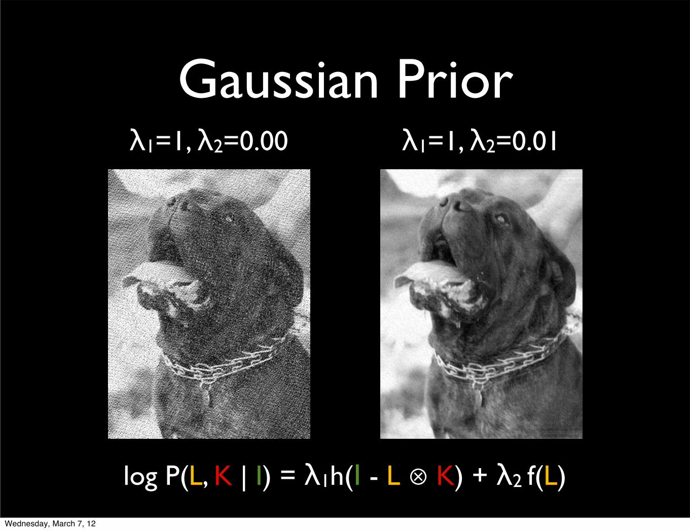
Gaussian Priorλ1=1, λ2=0.01λ1=1, λ2=0.00
log P(L, K | I) = λ1h(I - L ⊗ K) + λ2 f(L)
Wednesday, March 7, 12
Gaussian Prior
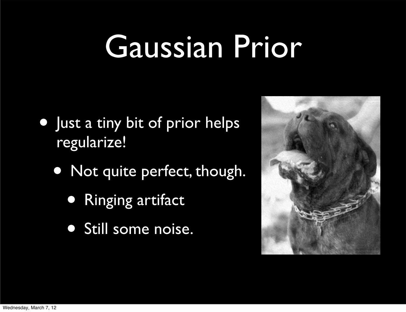
• Just a tiny bit of prior helps regularize!
• Not quite perfect, though.
• Ringing artifact
• Still some noise.
Wednesday, March 7, 12
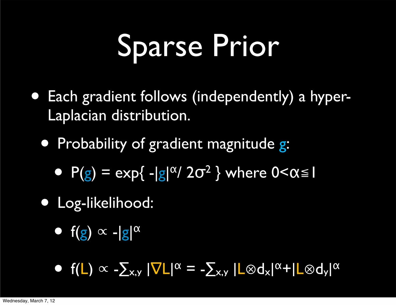
Sparse Prior
• Each gradient follows (independently) a hyper-Laplacian distribution.
• Probability of gradient magnitude g:
• P(g) = exp{ -|g|α/ 2σ2 } where 0<α≦1
• Log-likelihood:
• f(g) ∝ -|g|α
• f(L) ∝ -∑x,y |∇L|α = -∑x,y |L⊗dx|α+|L⊗dy|α
Wednesday, March 7, 12

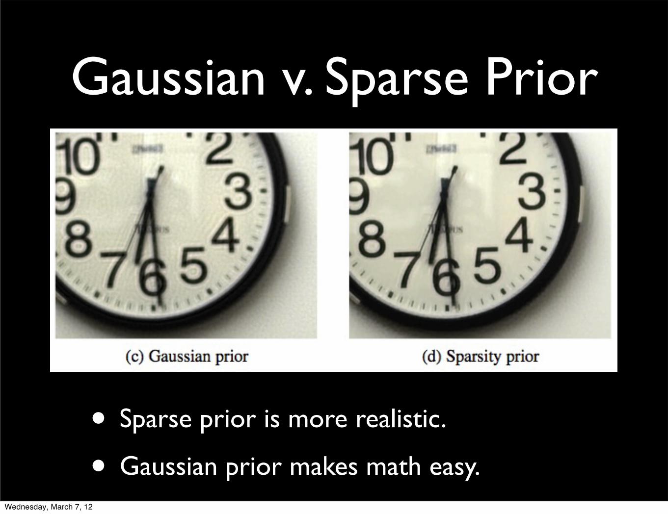
Gaussian v. Sparse Prior
• Sparse prior is more realistic.
• Gaussian prior makes math easy.Wednesday, March 7, 12
Gaussian v. Sparse Prior
• Sparse prior is more realistic.
• Gaussian prior makes math easy.Wednesday, March 7, 12
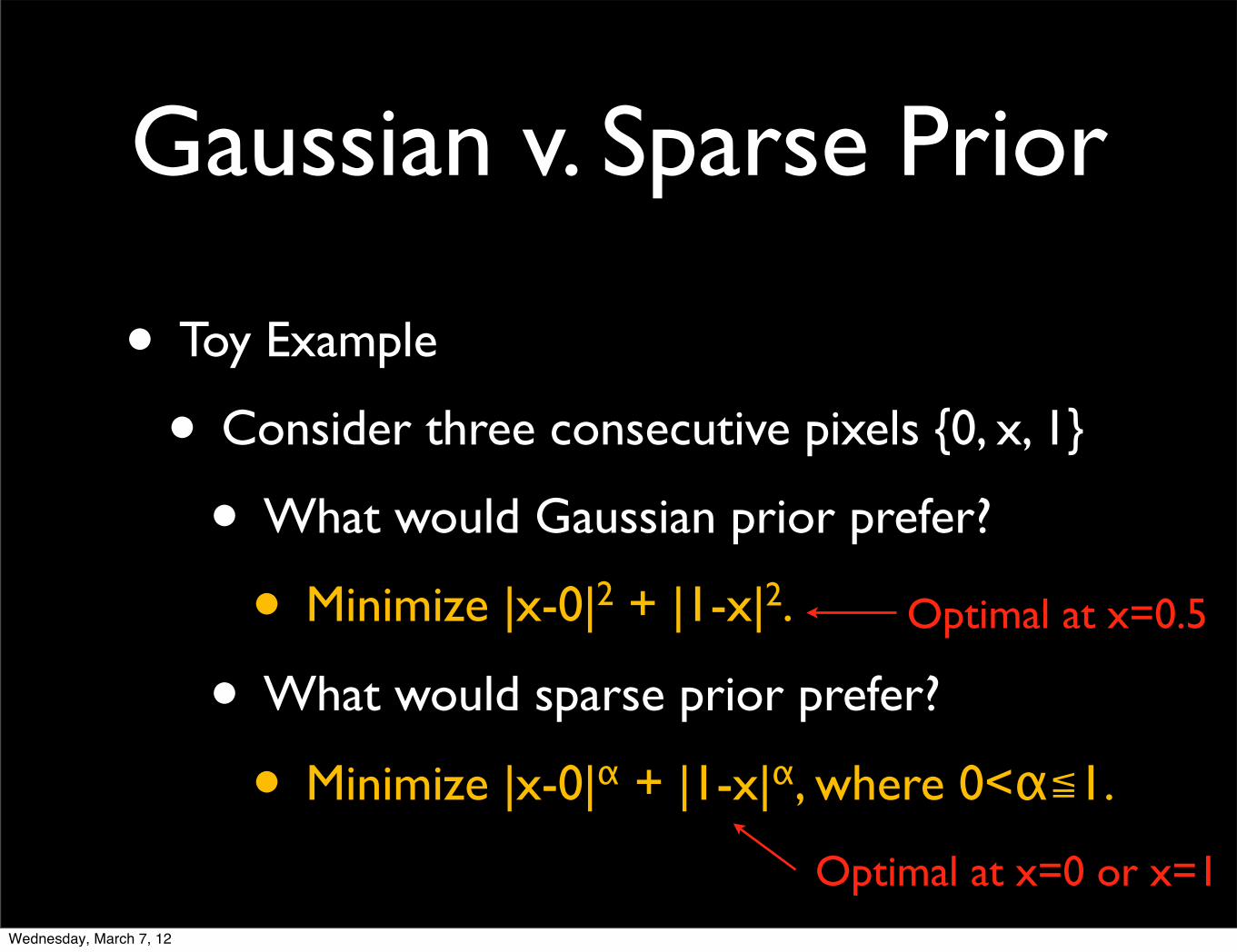
Gaussian v. Sparse Prior
• Toy Example
• Consider three consecutive pixels {0, x, 1}
• What would Gaussian prior prefer?
• Minimize |x-0|2 + |1-x|2.
• What would sparse prior prefer?
• Minimize |x-0|α + |1-x|α, where 0<α≦1.
Optimal at x=0.5
Optimal at x=0 or x=1Wednesday, March 7, 12
Blind Deconvolution
• We have so far assumed the blur kernel is known.
• True for coded aperture, or other calibrated blurs.
• True if kernel can be calculated somehow.
• Most of the time, the blur is unknown.
Wednesday, March 7, 12

Blind Deconvolution
• I = L ⊗ K + N
• Solve for the maximum likelihood (L, K)
• log P(L | K, I) =
λ1h(I - L ⊗ K) + λ2 f(L) + λ3 g(K)
• Every paper follows this recipe.
Data Term ImagePrior
KernelPrior
Wednesday, March 7, 12
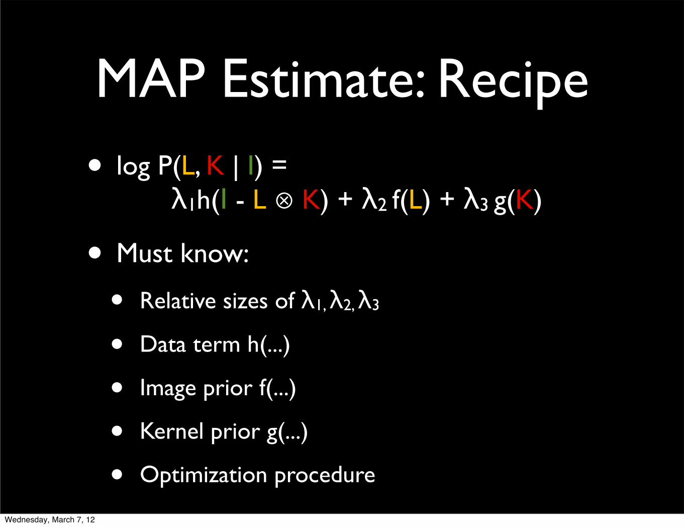
MAP Estimate: Recipe
• log P(L, K | I) = λ1h(I - L ⊗ K) + λ2 f(L) + λ3 g(K)
• Must know:
• Relative sizes of λ1, λ2, λ3
• Data term h(...)
• Image prior f(...)
• Kernel prior g(...)
• Optimization procedure
Wednesday, March 7, 12

Data Term : h(I - L ⊗ K)
• Penalize deviation from observed data.
• h(z) = |z|2 (Fergus 2005, Jia 2007, Krishnan 2010)
• Most obvious. Corresponds to Gaussian noise
• h(z) = |∇z|2 (Cho 2009)
• Cheap if you are already computing gradients.
• h(z) = |z|2 + |∇z|2 + ... (Shan 2008)
• Constrain multiple orders of derivatives.
Wednesday, March 7, 12
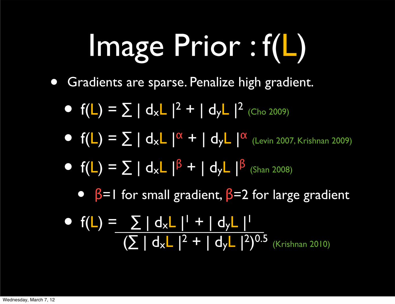
Image Prior : f(L)• Gradients are sparse. Penalize high gradient.
• f(L) = ∑ | dxL |2 + | dyL |2 (Cho 2009)
• f(L) = ∑ | dxL |α + | dyL |α (Levin 2007, Krishnan 2009)
• f(L) = ∑ | dxL |β + | dyL |β (Shan 2008)
• β=1 for small gradient, β=2 for large gradient
• f(L) = ∑ | dxL |1 + | dyL |1 (∑ | dxL |2 + | dyL |2)0.5 (Krishnan 2010)
Wednesday, March 7, 12
2 -1.5 -1 -0.5 0 0.5 1 1.5 2
-2.8
-2.4
-2
-1.6
-1.2
-0.8
-0.4
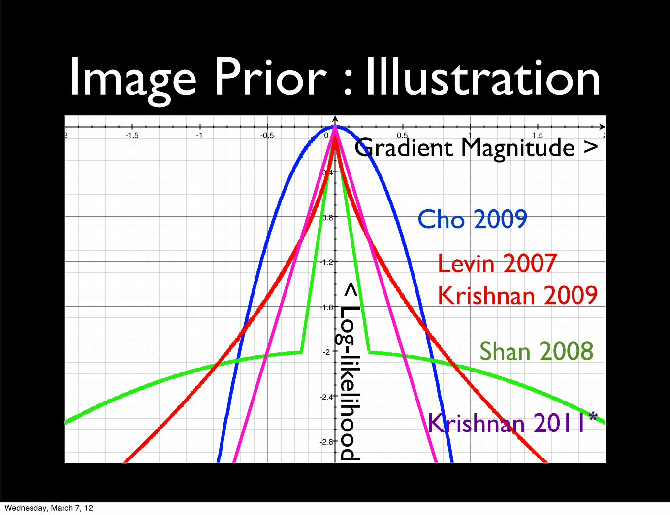
Image Prior : Illustration
< Log-likelihood
Gradient Magnitude >
Cho 2009
Levin 2007Krishnan 2009
Shan 2008
Krishnan 2011*
Wednesday, March 7, 12
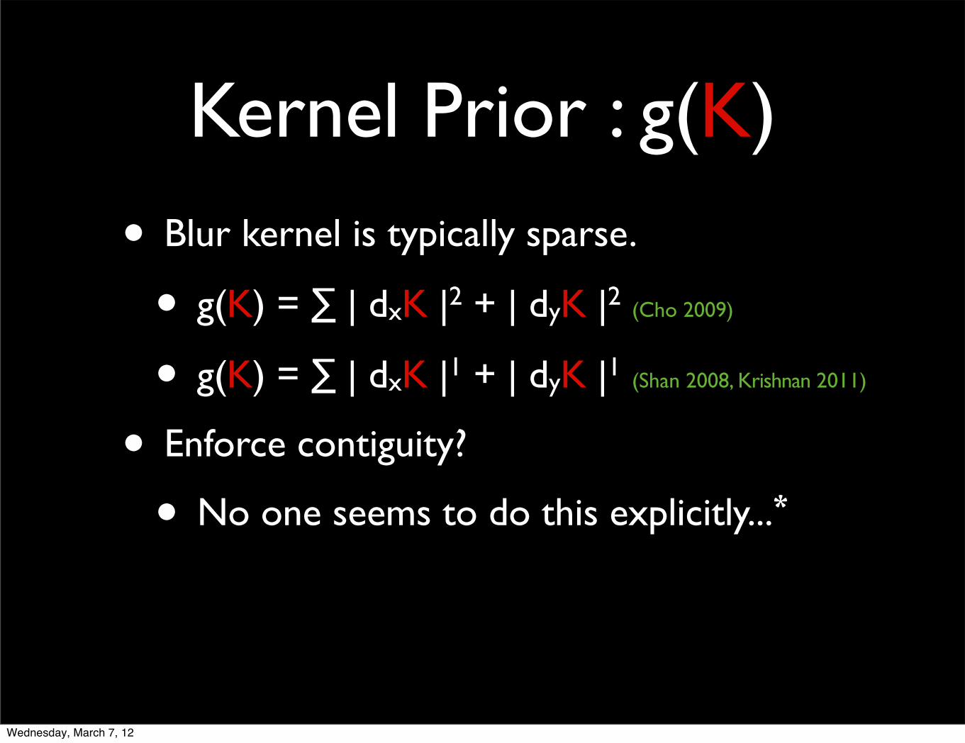
Kernel Prior : g(K)
• Blur kernel is typically sparse.
• g(K) = ∑ | dxK |2 + | dyK |2 (Cho 2009)
• g(K) = ∑ | dxK |1 + | dyK |1 (Shan 2008, Krishnan 2011)
• Enforce contiguity?
• No one seems to do this explicitly...*
Wednesday, March 7, 12

Optimization
• In the end, we have an objective function in terms of L and K.
• Quadratic in simplest form (Cho 2009)
• Standard linear system to solve. We saw this earlier.
• Mixture of quadratic and L1-norm (Shan 2008)
• Highly nonlinear (Krishnan 2011)
• Need fancier methods.
Wednesday, March 7, 12
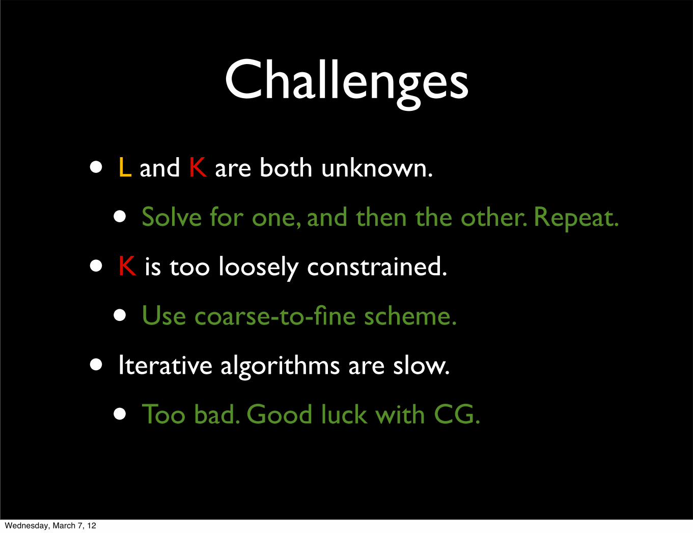
Challenges
• L and K are both unknown.
• Solve for one, and then the other. Repeat.
• K is too loosely constrained.
• Use coarse-to-fine scheme.
• Iterative algorithms are slow.
• Too bad. Good luck with CG.
Wednesday, March 7, 12

Generic Pseudocode(Fergus 2005, Shan 2008, Cho 2009, Krishnan 2011)
• From coarse to fine,
• Resample L, K, I to current scale.
• Fix L, and solve for K.
• Typically some sort of iterative solver.
• Fix K, and solve for L.
• Non-blind deconvolution.
Wednesday, March 7, 12

Coarse-to-Fine
Coarse-to-fine >
CG iterations >True kernel
Wednesday, March 7, 12

WithoutCoarse-to-Fine
Outer Iterations >
CG iterations >True kernel
Wednesday, March 7, 12

WithoutCoarse-to-Fine
Outer Iterations >
CG iterations >True kernel
Wednesday, March 7, 12
Case Study
• Cho and Lee, 2009
• (Comparatively) Very fast.
• Quality comparable to others. How?
Wednesday, March 7, 12

Case Study : Cho 2009
• log P(L, K | I) = λ1h(I - L ⊗ K) + λ2 f(L) + λ3 g(K)
• h is quadratic.
• L is quadratic.
• K is quadratic.
Optimizer’s paradise!
Wednesday, March 7, 12

Pseudocode
• From coarse to fine,
• Resample L, K, I to current scale.
• Fix L, and solve for K.
• Conjugate gradient.
• Fix K, and solve for L.
• Fourier-domain division
Bad. Creates ringing
Very fast
In Fourier domainas well
Wednesday, March 7, 12

Pseudocode
• From coarse to fine,
• Resample L, K, I to current scale.
• Fix L, and solve for K.
• Conjugate gradient.
• Fix K, and solve for L.
• Fourier-domain division
• Bilateral-filter and shock-filter L.
• Use a nice non-blind deconv. for final result.Wednesday, March 7, 12

De-Ringing
After shock-filterAfter bilateral filterDeconvolved result from previous scale (L)
Wednesday, March 7, 12
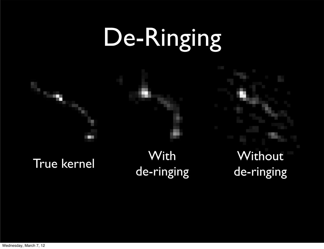
De-Ringing
True kernelWith
de-ringingWithoutde-ringing
Wednesday, March 7, 12
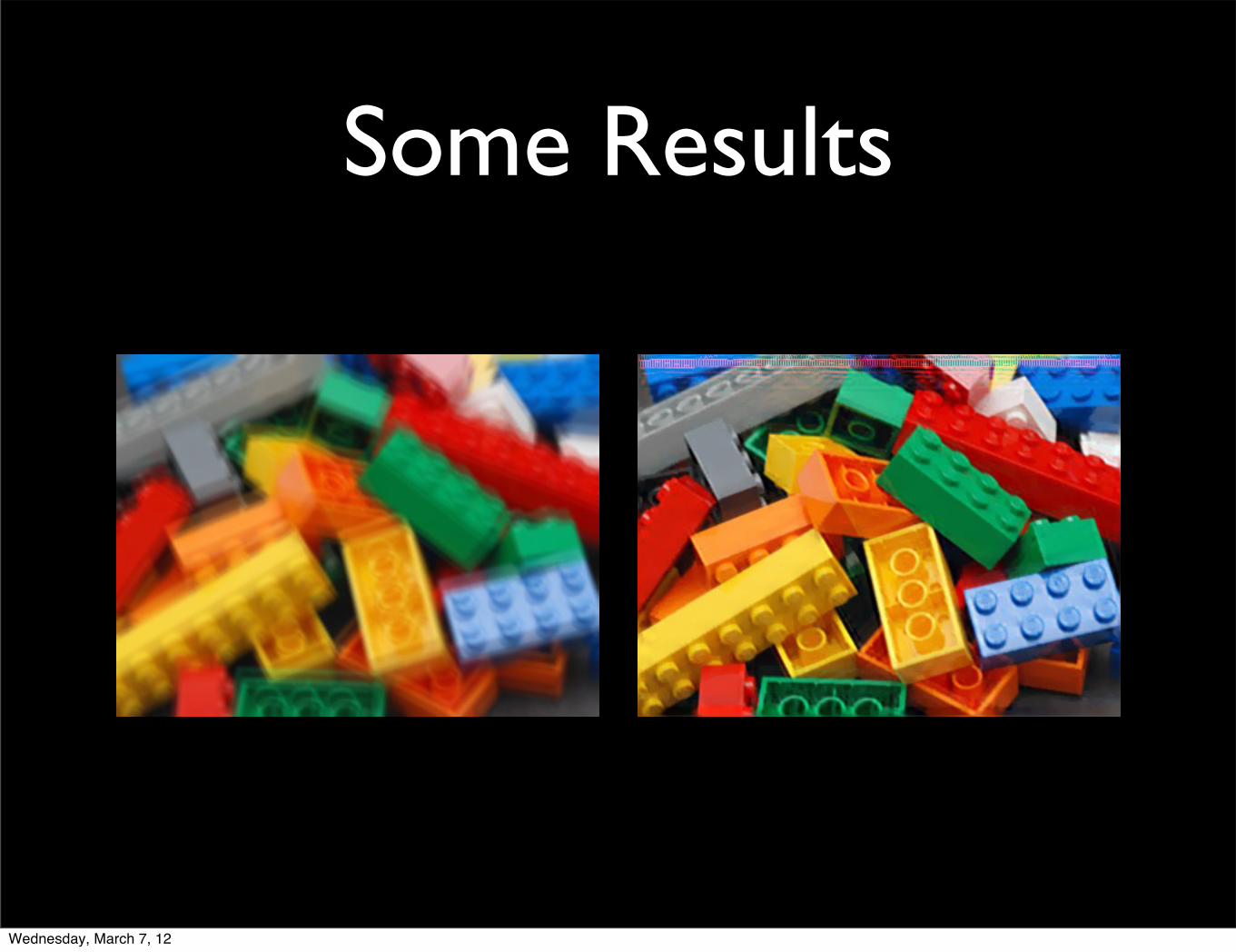
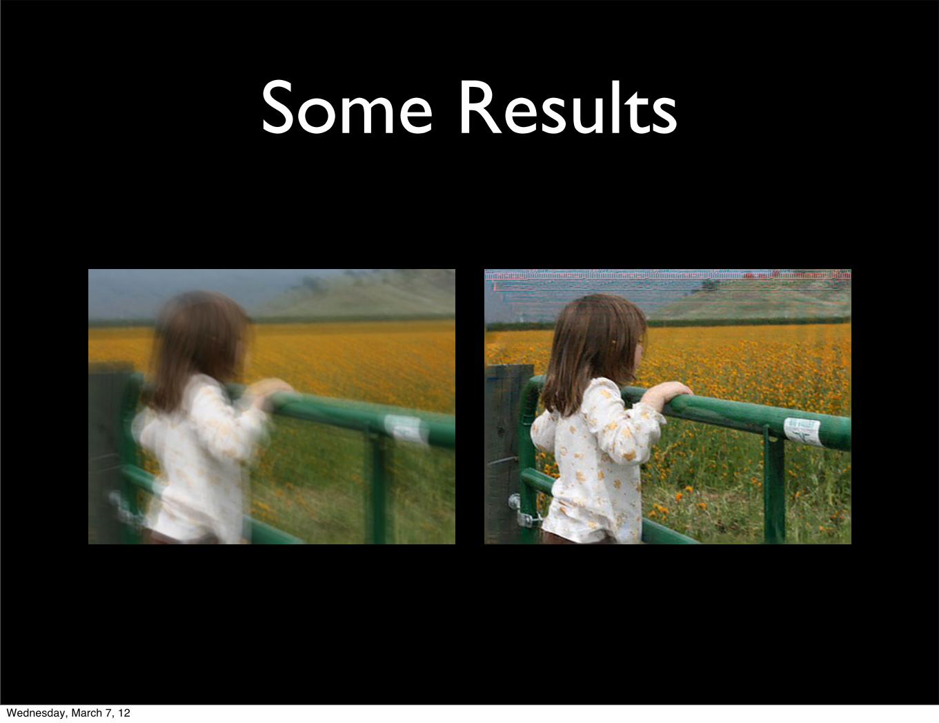
Some Results
Wednesday, March 7, 12
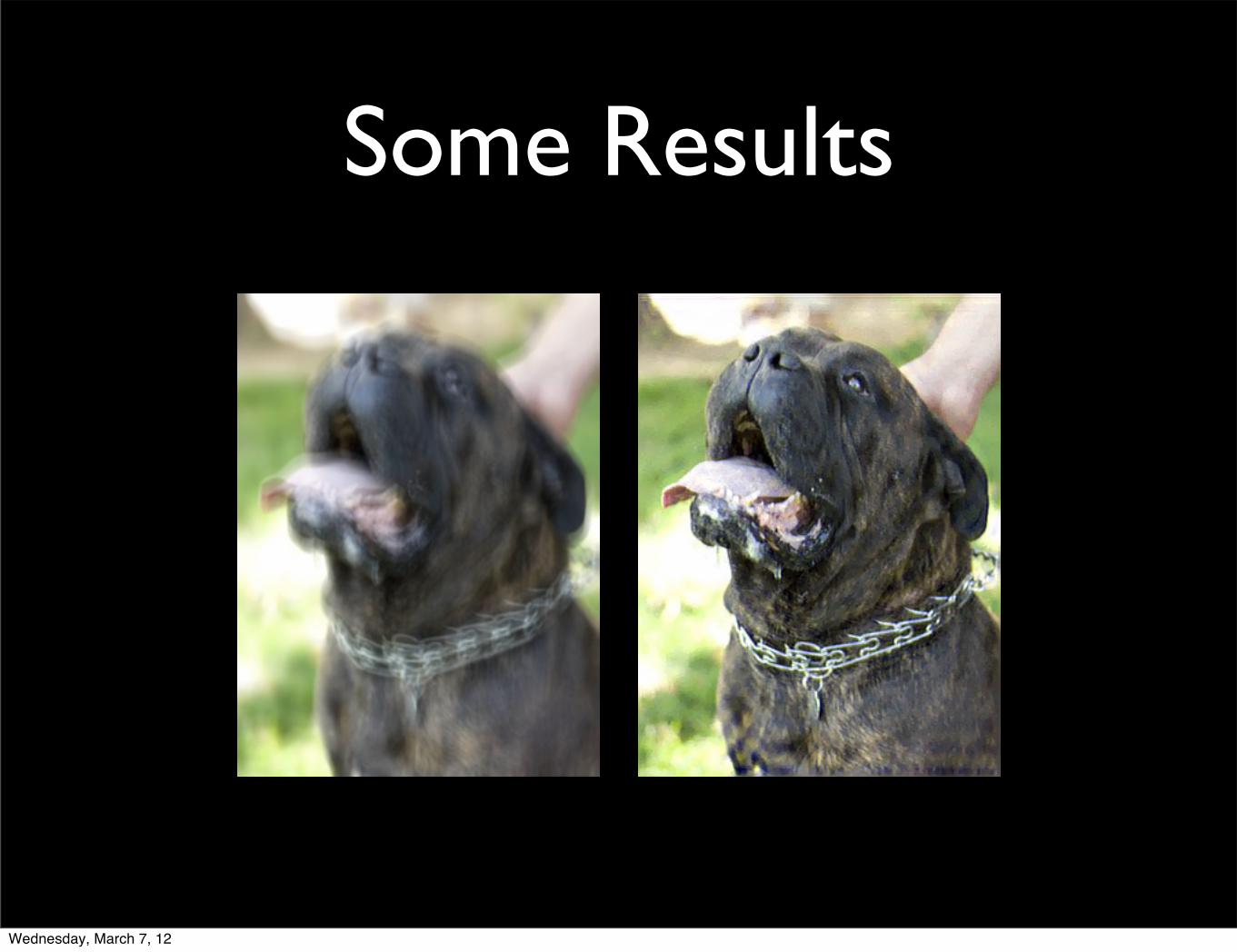
Some Results
Wednesday, March 7, 12
Some Results
Wednesday, March 7, 12

Performance Method Implementation Speed
Fergus 2006 Matlab 546 sec.
Shan 2008 Binary 121 sec.
Cho 2009 Binary 8 sec.
Krishnan 2011 Matlab 280 sec.
All tests on ~0.5MP images with 31x31 kernel
Wednesday, March 7, 12
Parameters, Parameters
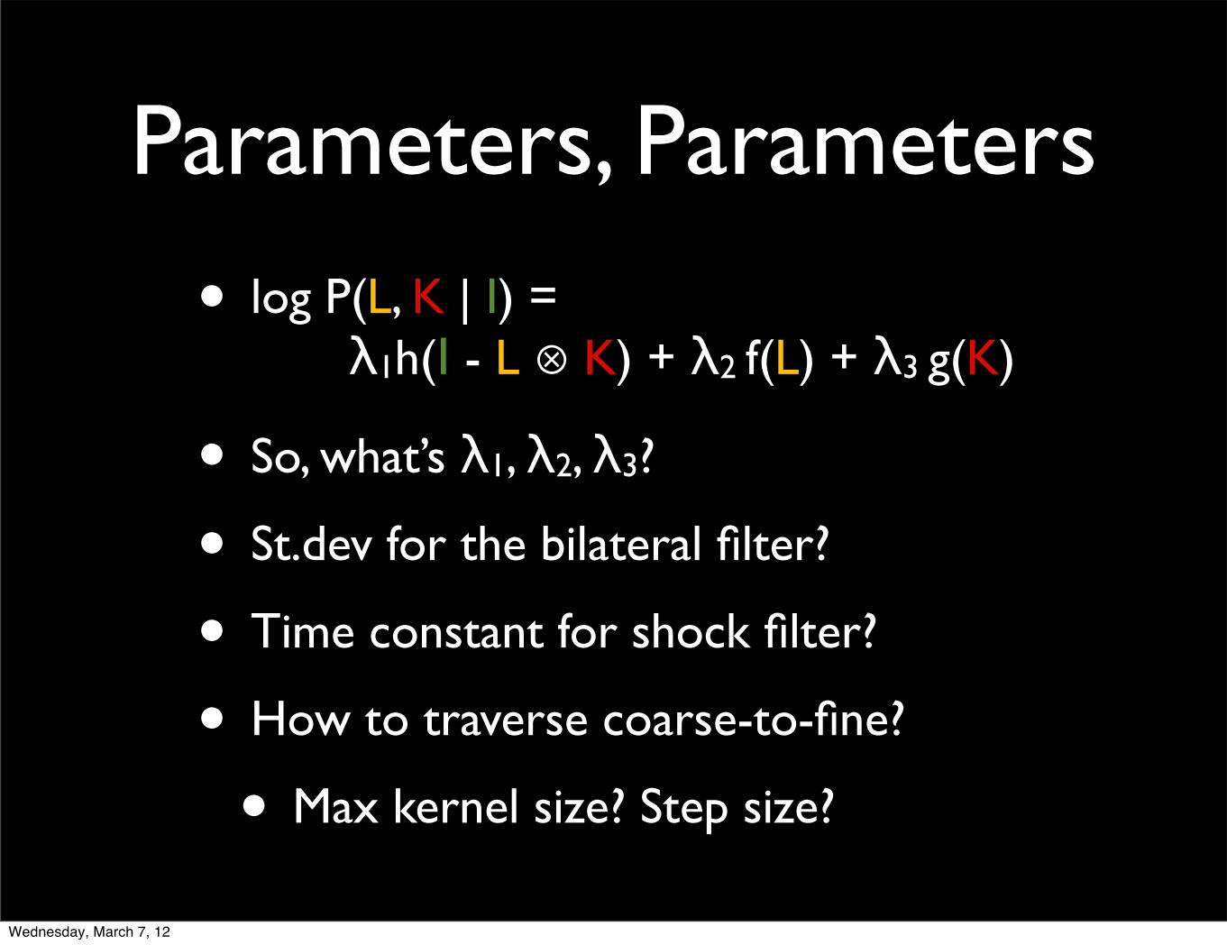
• log P(L, K | I) = λ1h(I - L ⊗ K) + λ2 f(L) + λ3 g(K)
• So, what’s λ1, λ2, λ3?
• St.dev for the bilateral filter?
• Time constant for shock filter?
• How to traverse coarse-to-fine?
• Max kernel size? Step size?
Wednesday, March 7, 12

Parameters, Parameters
• Demo script from Shan 2008
• deblur in1.png out1.png 27 27 0.010 0.2 1 0 0 0 0 3.5deblur in2.png out2.png 27 27 0.008 0.2 1 0 0 0 0 0.0
• Demo script from Cho 2009
• deblur in1.jpg out1.jpg 49 47 0.5 0.0005deblur in2.jpg out2.jpg 61 43 0.5 0.0005deblur in3.jpg out3.jpg 33 33 0.5 0.001deblur in4.jpg out4.jpg 35 49 0.5 0.0005deblur in5.jpg out5.jpg 65 93 0.5 0.0002
Wednesday, March 7, 12
Video
• First 30 seconds of
• http://www.youtube.com/watch?v=xxjiQoTp864
Wednesday, March 7, 12
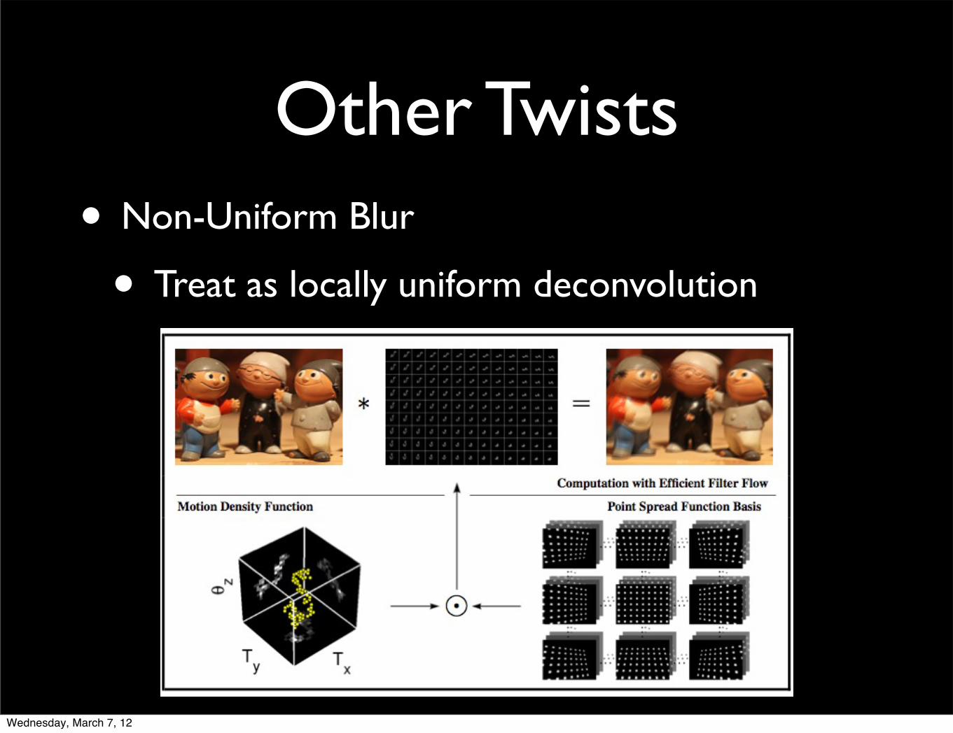
Other Twists• Non-Uniform Blur
• Treat as locally uniform deconvolution
Wednesday, March 7, 12
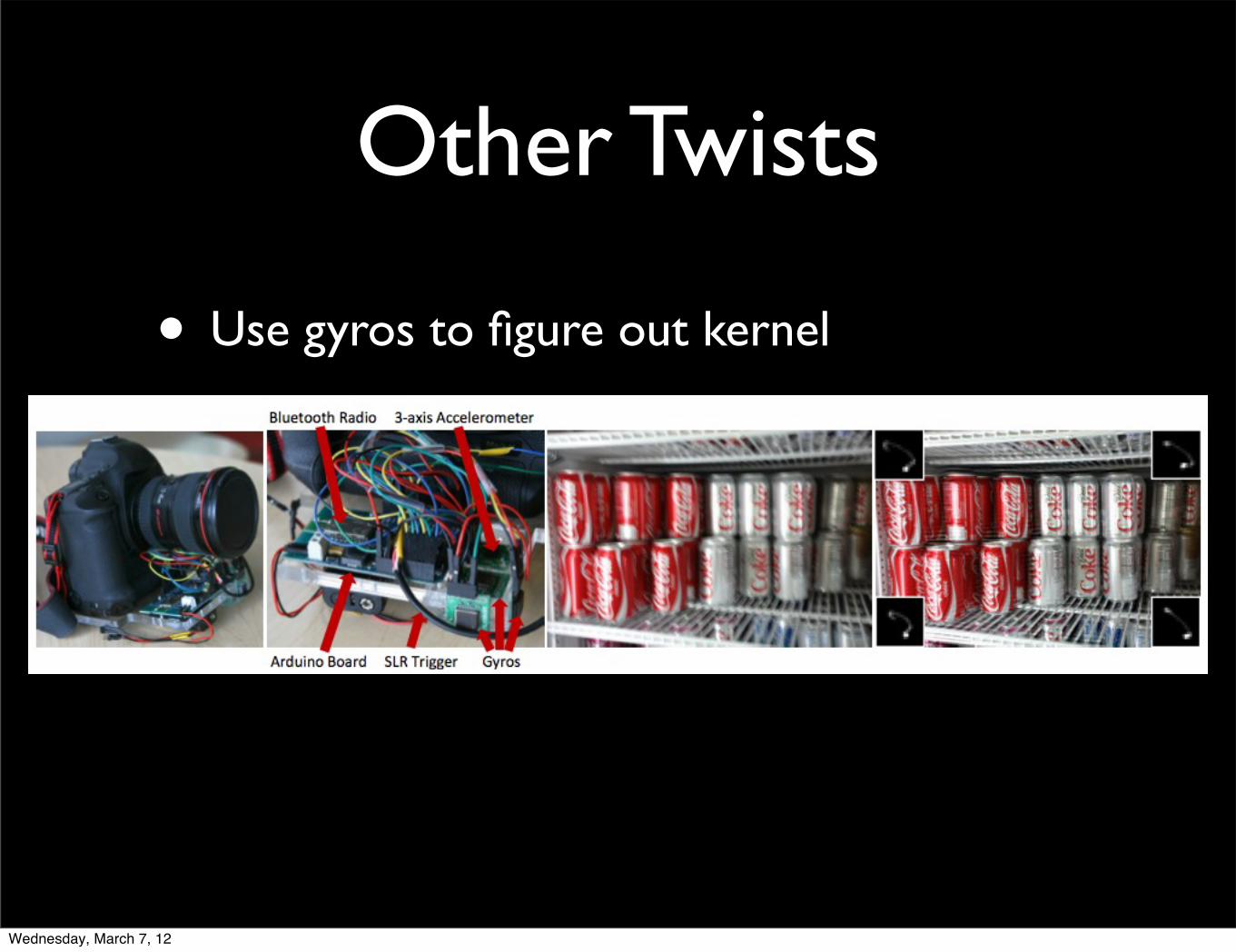
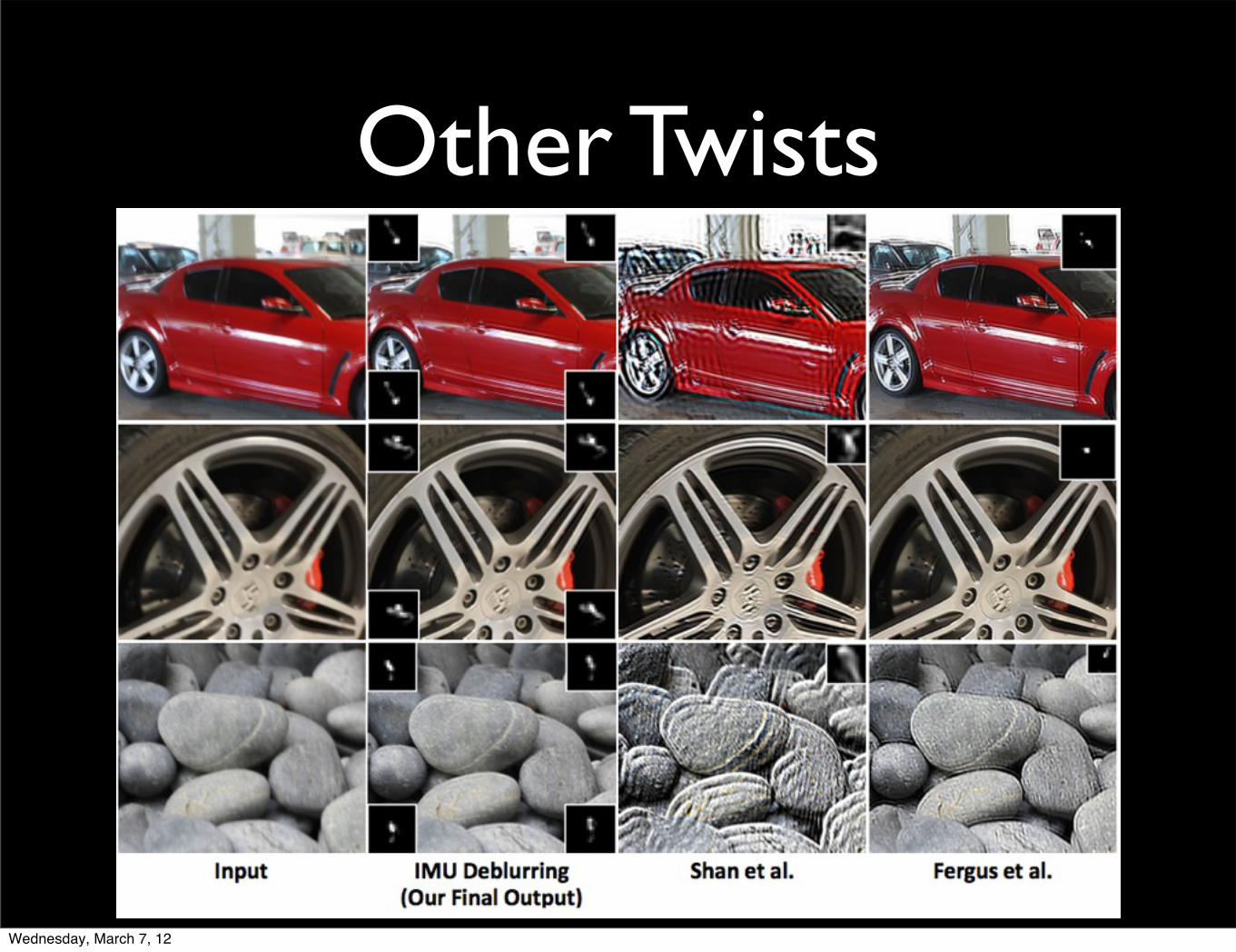
Other Twists
• Use gyros to figure out kernel
Wednesday, March 7, 12
Other Twists
Wednesday, March 7, 12

Alternatives
• Take a short exposure and denoise.
• Align-and-average
• People are studying the tradeoffs now.
Wednesday, March 7, 12

Questions?
Wednesday, March 7, 12
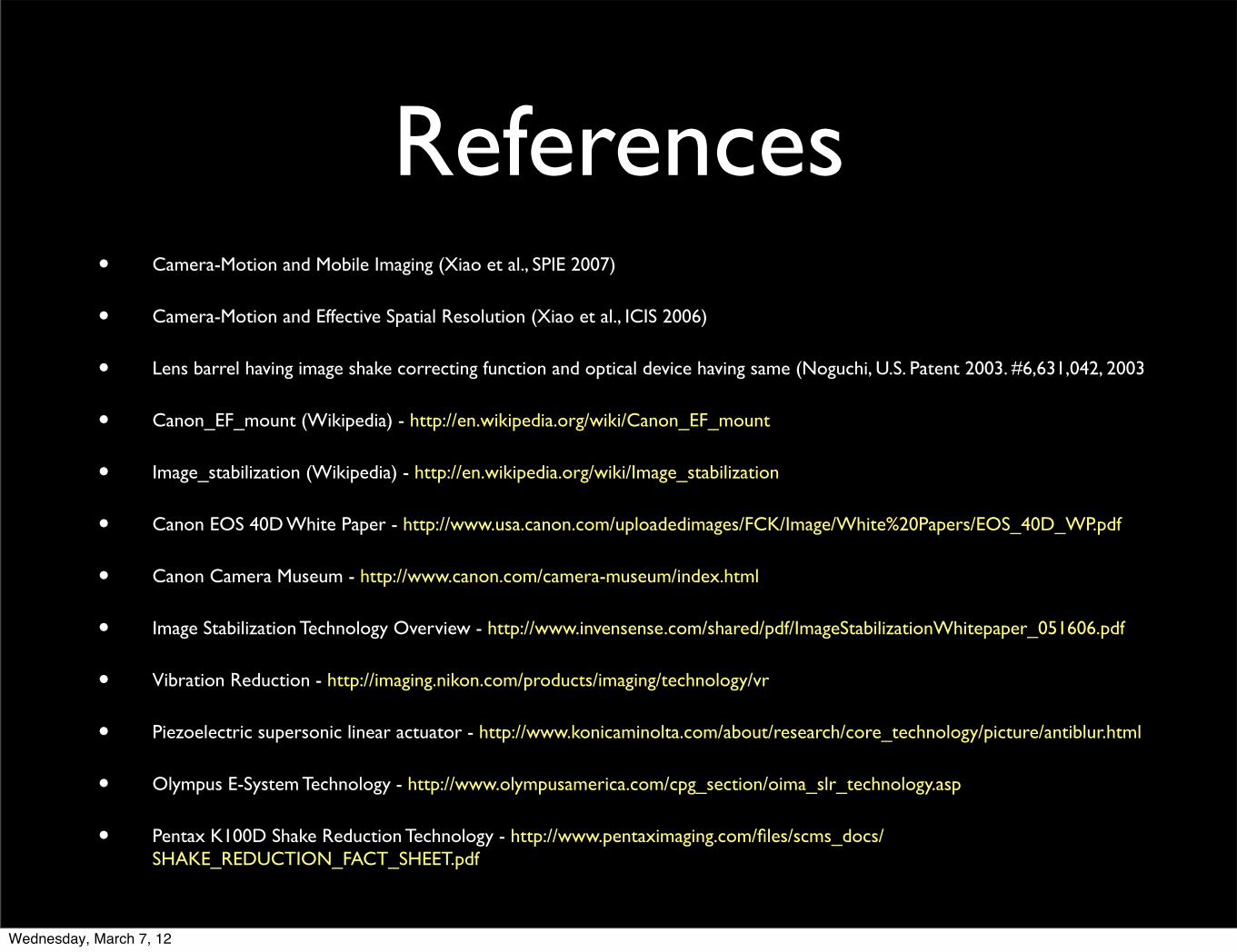
References• Camera-Motion and Mobile Imaging (Xiao et al., SPIE 2007)
• Camera-Motion and Effective Spatial Resolution (Xiao et al., ICIS 2006)
• Lens barrel having image shake correcting function and optical device having same (Noguchi, U.S. Patent 2003. #6,631,042, 2003
• Canon_EF_mount (Wikipedia) - http://en.wikipedia.org/wiki/Canon_EF_mount
• Image_stabilization (Wikipedia) - http://en.wikipedia.org/wiki/Image_stabilization
• Canon EOS 40D White Paper - http://www.usa.canon.com/uploadedimages/FCK/Image/White%20Papers/EOS_40D_WP.pdf
• Canon Camera Museum - http://www.canon.com/camera-museum/index.html
• Image Stabilization Technology Overview - http://www.invensense.com/shared/pdf/ImageStabilizationWhitepaper_051606.pdf
• Vibration Reduction - http://imaging.nikon.com/products/imaging/technology/vr
• Piezoelectric supersonic linear actuator - http://www.konicaminolta.com/about/research/core_technology/picture/antiblur.html
• Olympus E-System Technology - http://www.olympusamerica.com/cpg_section/oima_slr_technology.asp
• Pentax K100D Shake Reduction Technology - http://www.pentaximaging.com/files/scms_docs/SHAKE_REDUCTION_FACT_SHEET.pdf
Wednesday, March 7, 12
References
• Removing Camera Shake from a Single Photograph (Fergus et al., SIGGRAPH 2006)
• Image and Depth from a Conventional Camera with a Coded Aperture (Levin et al., SIGGRAPH 2007)
• High Quality Motion Deblurring from a Single Image (Shan et al., SIGGRAPH 2008)
• Fast Motion Deblurring (Cho and Lee, SIGGRAPH Asia 2009)
• Fast Image Deconvolution using Hyper-Laplacian Priors (Krishnan and Fergus, NIPS 2009)
• Non-Uniform Deblurring for Shaken Images (Whyte et al., CVPR 2010)
• Image Deblurring using Inertial Measurement Sensors (Joshi et al., SIGGRAPH 2010)
• Blind Deconvolution Using a Normalized Sparsity Measure (Krishnan et al., CVPR 2011)
• Fast Removal of Non-Uniform Camera Shake (Hirsch et al., ICCV 2011)
Wednesday, March 7, 12