computational science and engineering (international master’s … · 2019-05-23 · 8. effect of...

Computational Science and Engineering(International Master’s Program)

Technische Universitat Munchen

Master’s Thesis

Implementation and Evaluation ofMLEM-Algorithm on GPU using CUDA

Apoorva Gupta

Computational Science and Engineering(International Master’s Program)

Technische Universitat Munchen

Master’s Thesis

Implementation and Evaluation of MLEM-Algorithm onGPU using CUDA

Author: Apoorva Gupta1st examiner: Prof. Dr. rer. nat. Martin Schulz

2nd examiner: PD Dr. rer. nat. habil. Josef WeidendorferAssistant advisors: M.Sc. Dai Yang

Dipl.-Tech. Math. (Univ.) Tilman KustnerSubmission Date: May 15th, 2018

I hereby declare that this thesis is entirely the result of my own work except where other-wise indicated. I have only used the resources given in the list of references.

May 15th, 2018 Apoorva Gupta

Acknowledgments

First, I would like to thank Prof. Martin Schulz to initially give me various options tochoose from for my master’s thesis and to later agree to supervise the chosen one. Hisregular guidance and inputs helped me to explore the unknown and improve the qualityof work many-folds.

I could not be more thankful to Dr. Josef Weidendorfer for agreeing to also supervise thethesis.

I would like to also thank Dai Yang and Tilman Kustner without their support this thesiswould not have been possible. They have never once hesitated to provide me the help thatI needed while writing the thesis and have been very patient to pass on their knowledgeand experience no matter how embarrassing my queries were.

I would also like to take this opportunity to thank Leibniz Supercomputing Center(LRZ)to grant me the access to the best possible resources in the form of MAC Cluster and theDGX-1 machine, with the help of which I could test my assumptions and which made thethesis even more interesting. I would not have been able to accomplish the work withoutthe very helpful documentation of CUDA, CuBLAS, CuSparse, NVML libraries and theequally helpful CUDA forum maintained by NVIDIA.

Lastly, a big thanks goes to my Mother and Father for their unwavering belief in me andthe support they have provided, especially during the moments of adversity, which hashelped me to come back stronger every time.

vii

”Redesigning your application to run multithreaded on a multicore machine is a little like learningto swim by jumping into the deep end.”

-Herb Sutter

viii

Abstract

With the release of CUDA, a parallel computing platform and application programminginterface (API) model, in 2007 by NVIDIA the learning curve to code on the GPUs havedrastically reduced. Along with the performance benefits the use of GPU promises for avariety of applications, it has become very enticing for the software developers and re-searchers to make use of this new hardware/software stack for faster feedback to theirproblems.

This thesis is an attempt to solve the computationally expensive Maximum LikelihoodExpectation Maximization (MLEM) algorithm with respect to the image reconstructionin Positron Emission Tomography (PET). The CuBLAS, CuSparse and NVML libraries,provided by NVIDIA, have been extensively used to run the algorithm and to harness thefull power of the GPUs.

The most expensive operation in the entire process is the transpose Sparse Matrix VectorMultiplication(SPMV T) for which the functions provided by the CuSparse libraries wereused and which were later bench-marked against the custom kernels developed duringthe thesis. Apart from that the effect of multi GPU, Cuda Aware MPI, pinned memory andhybrid computing have also been studied with respect to the performance and accuracy ofthe results.

Finally, the last section has been dedicated to the discussion of the limitations of presentimplementation and how those limitations could be overcome by making the code re-source aware. It also discusses how the performance of the code could be improved byusing the merge based SPMV to rewrite the most expensive loop operation i.e. SPMV T.

ix

Contents

AcknowledgementsAcknowledgements vii

AbstractAbstract ix

I. Introduction and Background TheoryI. Introduction and Background Theory 1

1. PET Image Reconstruction1. PET Image Reconstruction 2

2. Related Work2. Related Work 4

3. MLEM Algorithm and System Matrix3. MLEM Algorithm and System Matrix 5

4. Sparse Matrix Format, SPMV and SPMV T4. Sparse Matrix Format, SPMV and SPMV T 104.1. Sparse Matrix Vector Multiplication(SPMV)4.1. Sparse Matrix Vector Multiplication(SPMV) . . . . . . . . . . . . . . . . . . . 114.2. Transpose Sparse Matrix Vector Multiplication(SPMV T)4.2. Transpose Sparse Matrix Vector Multiplication(SPMV T) . . . . . . . . . . . 12

5. GPU Architecture and Programming5. GPU Architecture and Programming 145.1. Grids, Blocks and Threads5.1. Grids, Blocks and Threads . . . . . . . . . . . . . . . . . . . . . . . . . . . . . 155.2. Register, Local, Constant, Shared, Global, and Texture memory5.2. Register, Local, Constant, Shared, Global, and Texture memory . . . . . . . . 175.3. Host, Device and Global Kernels5.3. Host, Device and Global Kernels . . . . . . . . . . . . . . . . . . . . . . . . . 195.4. Streams and Events5.4. Streams and Events . . . . . . . . . . . . . . . . . . . . . . . . . . . . . . . . . 195.5. Asynchronous Kernels and Copy Operations5.5. Asynchronous Kernels and Copy Operations . . . . . . . . . . . . . . . . . . 195.6. Atomic Operations5.6. Atomic Operations . . . . . . . . . . . . . . . . . . . . . . . . . . . . . . . . . 205.7. Error Checking5.7. Error Checking . . . . . . . . . . . . . . . . . . . . . . . . . . . . . . . . . . . 205.8. Coalesced Memory Access5.8. Coalesced Memory Access . . . . . . . . . . . . . . . . . . . . . . . . . . . . . 215.9. Pinned Memory5.9. Pinned Memory . . . . . . . . . . . . . . . . . . . . . . . . . . . . . . . . . . . 235.10. Bank Conflicts5.10. Bank Conflicts . . . . . . . . . . . . . . . . . . . . . . . . . . . . . . . . . . . . 23

6. Other Terminologies6. Other Terminologies 256.1. Heterogeneous Computing6.1. Heterogeneous Computing . . . . . . . . . . . . . . . . . . . . . . . . . . . . 256.2. CUDA Aware MPI6.2. CUDA Aware MPI . . . . . . . . . . . . . . . . . . . . . . . . . . . . . . . . . 256.3. Floating Point Arithmetic6.3. Floating Point Arithmetic . . . . . . . . . . . . . . . . . . . . . . . . . . . . . 27

x

Contents

II. Experiments and ResultsII. Experiments and Results 31

7. Benchmarking MAC Cluster7. Benchmarking MAC Cluster 32

8. Effect of Cuda Aware MPI, Pinned Memory and Custom Kernels8. Effect of Cuda Aware MPI, Pinned Memory and Custom Kernels 34

9. Effect of Splitting Work between CPU and GPU9. Effect of Splitting Work between CPU and GPU 39

10. Performance vs Number of GPU10. Performance vs Number of GPU 43

11. Performance on CPU vs OpenMP Threads11. Performance on CPU vs OpenMP Threads 47

12. Compilation for Specific Architecture12. Compilation for Specific Architecture 50

13. Profiling using NVVP13. Profiling using NVVP 52

III. Future Work and ConclusionIII. Future Work and Conclusion 54

14. Future Work14. Future Work 5514.1. Resource Aware Computing14.1. Resource Aware Computing . . . . . . . . . . . . . . . . . . . . . . . . . . . . 5514.2. Merge Based CsrMV14.2. Merge Based CsrMV . . . . . . . . . . . . . . . . . . . . . . . . . . . . . . . . 57

15. Conclusion15. Conclusion 59

AppendixAppendix 62

A. Computational ResourcesA. Computational Resources 62A.1. DGX-1A.1. DGX-1 . . . . . . . . . . . . . . . . . . . . . . . . . . . . . . . . . . . . . . . . 62A.2. Mac ClusterA.2. Mac Cluster . . . . . . . . . . . . . . . . . . . . . . . . . . . . . . . . . . . . . 64

B. Compiling and Using CUDA Aware OpenMPI on Mac ClusterB. Compiling and Using CUDA Aware OpenMPI on Mac Cluster 65

C. Compiling NVML library on Mac ClusterC. Compiling NVML library on Mac Cluster 66

D. Notes on MLEM ImplementationD. Notes on MLEM Implementation 67

BibliographyBibliography 69

xi

Part I.

Introduction and Background Theory

1

1. PET Image Reconstruction

The Positron Emission Topography(PET) is a nuclear medicine imaging technique used tomeasure the physiological function by looking at blood flow, metabolism, neurotransmit-ters and radio-labelled drugs. In this process the tracer injected into the body of a livingsubject typically contains a small amount of radio-nuclides, like carbon-11 and nitrogen-13, having a short half life. Nowadays these PET scanners are used in different field ofmedicines namely Oncology, Neuro-imaging, Infectious diseases etc.[11]

A PET scanner consists of number of fixed detectors usually arranged in a ring aroundthe subject injected with the tracer. As the tracer undergoes positron emission decay itemits a positron. As the positron travels into the subject’s body it loses its kinetic energyand is finally able to interact with a electron in the body which ultimately leads to theemission of two gamma photons of 511 keV which travel into approximately opposite di-rections. If these emitted gamma photons are detected by the detectors (in approximatelyopposite direction) in a short time window (typically of a few nanoseconds) then the eventis recorded as positive else the detection is discarded. [22, 33]

Figure 1.1.: Configuration of MADPET-II[33]

Now since the emitted gamma photons travel almost 180 degrees to each other, it is pos-sible to localize their source along the straight line of coincidence which is typically calledthe Line of Response(LOR). The more the number of detectors the more the number of de-tected events which ultimately leads to better quality of the measurements. The coverage

2

of the three-dimensional space of interest, i.e. Field of View(FOV), by the LOR affects theachievable resolution. [11]

A possible configuration of an experimental small animal PET scanner (see Figure 1.11.1)developed at the Department of Nuclear Medicine, Technische Universitat Munchen adds asecond ring of gamma photons detectors which leads to better spatial resolution. Theadditional ring quadruples the amount of measured data and increases the computationaldemand of post processing step significantly for 3D image reconstruction.

3

2. Related Work

There have been several algorithms made available over the years to reconstruct the orig-inal PET images. All these algorithms could be classified under 2 major categories i.e.Analytic and Iterative. A comprehensive overview along with the mathematical founda-tion for both analytic and iterative algorithms has been given in [44].

The most widely used analytic PET image reconstruction algorithm is Filtered Back Pro-jection (FBP). Since the analytic algorithms are linear they are very helpful in quantitativedata analysis by allowing an easier control over the spatial resolution and noise correla-tions, they have remain important even today.

The noise introduced during the data collection in PET scanners due to the gamma pho-tons either not travelling 180 degrees apart or because of they being registered incorrectlyby the detectors leads to the FBP not performing very well with respect to the noise inthe measured data and it ultimately throws up artifacts in the reconstructed images. Thisproblem could be corrected upto a certain extent by pre-processing the data before imagereconstruction.[11]

The two widely used iterative algorithms are Maximum Likelihood Expectation Maximiza-tion (MLEM) which was first developed by Shepp and Vardi in 1982[55] and Ordered SubsetExpectation Maximization (OSEM) developed by Hudson and Larkin in 1994 [66].

The MLEM algorithm is a standard statistical estimation method. It works by taking aninitial guess of the image to be reconstructed and in each iteration maximizes the likelihoodfunction. While the MLEM algorithm provides a consistent and predictable convergenceresults, it is much more computationally expensive compared to FBP.

The OSEM algorithm partitions the data into multiple subsets which are mutually ex-clusive and it uses only one subset of data for each update. This has the benefit that eachpass over the entire data involves a greater number of updates, which leads to significantacceleration over MLEM.

The different possible splitting of the matrix for parallelization has been discussed ingreat detail by Chen and Lee [77] while the performance difference between OSEM andMLEM has been compared by Lalush and Tsui [88].

4

3. MLEM Algorithm and System Matrix

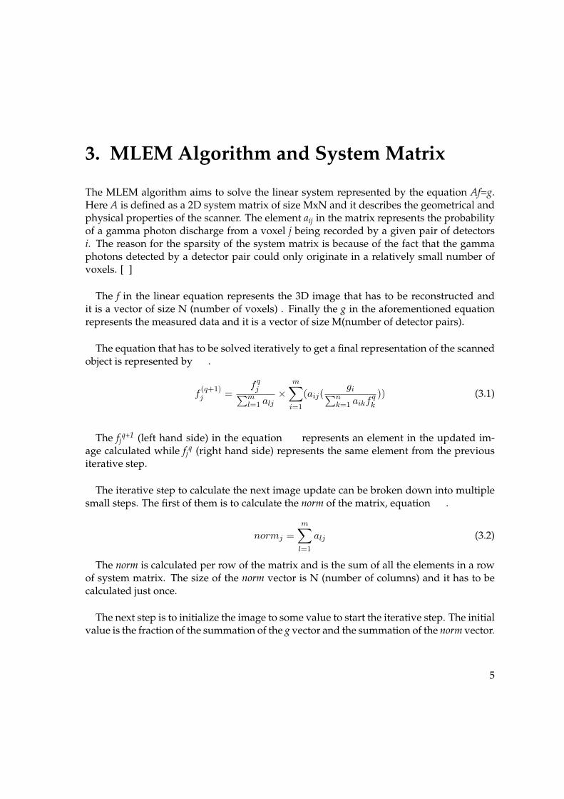
The MLEM algorithm aims to solve the linear system represented by the equation Af=g.Here A is defined as a 2D system matrix of size MxN and it describes the geometrical andphysical properties of the scanner. The element aij in the matrix represents the probabilityof a gamma photon discharge from a voxel j being recorded by a given pair of detectorsi. The reason for the sparsity of the system matrix is because of the fact that the gammaphotons detected by a detector pair could only originate in a relatively small number ofvoxels. [33]

The f in the linear equation represents the 3D image that has to be reconstructed andit is a vector of size N (number of voxels) . Finally the g in the aforementioned equationrepresents the measured data and it is a vector of size M(number of detector pairs).

The equation that has to be solved iteratively to get a final representation of the scannedobject is represented by 3.13.1.

f(q+1)j =

f qj∑ml=1 alj

×m∑i=1

(aij(gi∑n

k=1 aikfqk

)) (3.1)

The fjq+1 (left hand side) in the equation 3.13.1 represents an element in the updated im-age calculated while fjq (right hand side) represents the same element from the previousiterative step.

The iterative step to calculate the next image update can be broken down into multiplesmall steps. The first of them is to calculate the norm of the matrix, equation 3.23.2.

normj =m∑l=1

alj (3.2)

The norm is calculated per row of the matrix and is the sum of all the elements in a rowof system matrix. The size of the norm vector is N (number of columns) and it has to becalculated just once.

The next step is to initialize the image to some value to start the iterative step. The initialvalue is the fraction of the summation of the g vector and the summation of the norm vector.

5


The equation 3.33.3 shows this step it in a mathematical form.

fk =

∑mi=1 gi∑n

j=1 normj(3.3)

The next step is called the Forward Projection (FP), equation 3.43.4 , and it involves themultiplication of the system matrix A with the image vector f q. This step leads to thegeneration of a vector fwproj of size M (number of rows).

fwproji =n∑

k=1

aikfqk (3.4)

The next step in the quest is a scaling step, equation 3.53.5. In this step each element in themeasured data vector g is divided by the corresponding element in the vector fwproj. Thevector generated after this step is called correlation and is of size M (number of rows).

correlationi =gi

fwproji(3.5)

After calculating the correlation, the forward projection is compared to the actual mea-surement and a correction factor is derived, equation 3.63.6. This step is called the BackwardProjection (BP) and is equivalent to a transpose sparse matrix vector multiplication andleads to the generation of the update vector of size N (number of columns).

updatej =m∑l=1

aijcorrelationi (3.6)

Finally the result from backward projection is used to scale the image vector from theprevious iteration to give us the newly updated image, equation 3.73.7.

f(q+1)j =

f qjnormj

× updatej (3.7)

The entire algorithm has been presented as a pseudo code in 11. The steps in lines 1-17refers to the operations that have to be performed just once and it includes setting up theenvironment, allocation and initialization of the necessary vectors. The steps in lines 18-28are performed based on the number of iterations required and in these steps the imageis continuously updated. The Image Sum in line 24 is calculated by summing up all thevalues in the newly updated image vector f and it helps to check if the image is updating

6

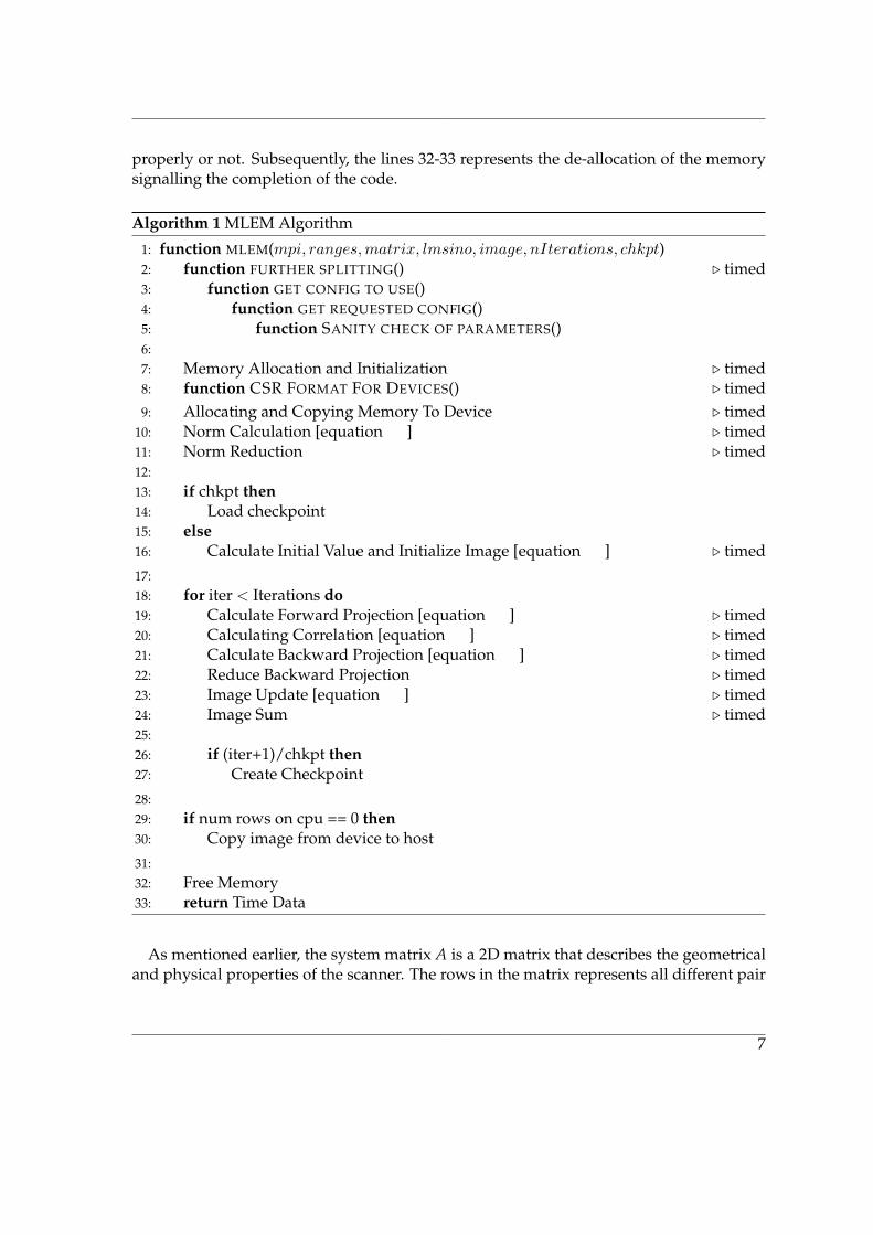
properly or not. Subsequently, the lines 32-33 represents the de-allocation of the memorysignalling the completion of the code.

Algorithm 1 MLEM Algorithm

1: function MLEM(mpi, ranges,matrix, lmsino, image, nIterations, chkpt)2: function FURTHER SPLITTING() . timed3: function GET CONFIG TO USE()4: function GET REQUESTED CONFIG()5: function SANITY CHECK OF PARAMETERS()6:7: Memory Allocation and Initialization . timed8: function CSR FORMAT FOR DEVICES() . timed9: Allocating and Copying Memory To Device . timed

10: Norm Calculation [equation 3.23.2] . timed11: Norm Reduction . timed12:13: if chkpt then14: Load checkpoint15: else16: Calculate Initial Value and Initialize Image [equation 3.33.3] . timed17:18: for iter < Iterations do19: Calculate Forward Projection [equation 3.63.6] . timed20: Calculating Correlation [equation 3.53.5] . timed21: Calculate Backward Projection [equation 3.63.6] . timed22: Reduce Backward Projection . timed23: Image Update [equation 3.73.7] . timed24: Image Sum . timed25:26: if (iter+1)/chkpt then27: Create Checkpoint28:29: if num rows on cpu == 0 then30: Copy image from device to host31:32: Free Memory33: return Time Data

As mentioned earlier, the system matrix A is a 2D matrix that describes the geometricaland physical properties of the scanner. The rows in the matrix represents all different pair

7


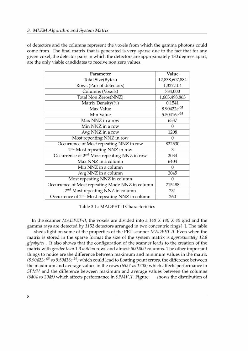
of detectors and the columns represent the voxels from which the gamma photons couldcome from. The final matrix that is generated is very sparse due to the fact that for anygiven voxel, the detector pairs in which the detectors are approximately 180 degrees apart,are the only viable candidates to receive non zero values.

Parameter ValueTotal Size(Bytes) 12,838,607,884

Rows (Pair of detectors) 1,327,104Columns (Voxels) 784,000

Total Non Zeros(NNZ) 1,603,498,863Matrix Density(%) 0.1541

Max Value 8.90422e-05

Min Value 5.50416e-24

Max NNZ in a row 6537Min NNZ in a row 0Avg NNZ in a row 1208

Most repeating NNZ in row 0Occurrence of Most repeating NNZ in row 822530

2nd Most repeating NNZ in row 3Occurrence of 2nd Most repeating NNZ in row 2034

Max NNZ in a column 6404Min NNZ in a column 0Avg NNZ in a column 2045

Most repeating NNZ in column 0Occurrence of Most repeating Mode NNZ in column 215488

2nd Most repeating NNZ in column 231Occurrence of 2nd Most repeating NNZ in column 260

Table 3.1.: MADPET-II Characteristics

In the scanner MADPET-II, the voxels are divided into a 140 X 140 X 40 grid and thegamma rays are detected by 1152 detectors arranged in two concentric rings[33]. The table3.13.1 sheds light on some of the properties of the PET scanner MADPET-II. Even when thematrix is stored in the sparse format the size of the system matrix is approximately 12.8gigabytes . It also shows that the configuration of the scanner leads to the creation of thematrix with greater than 1.3 million rows and almost 800,000 columns. The other importantthings to notice are the difference between maximum and minimum values in the matrix(8.90422e-05 vs 5.50416e-24) which could lead to floating point errors, the difference betweenthe maximum and average values in the rows (6537 vs 1208) which affects performance inSPMV and the difference between maximum and average values between the columns(6404 vs 2045) which affects performance in SPMV T. Figure 3.13.1 shows the distribution of

8

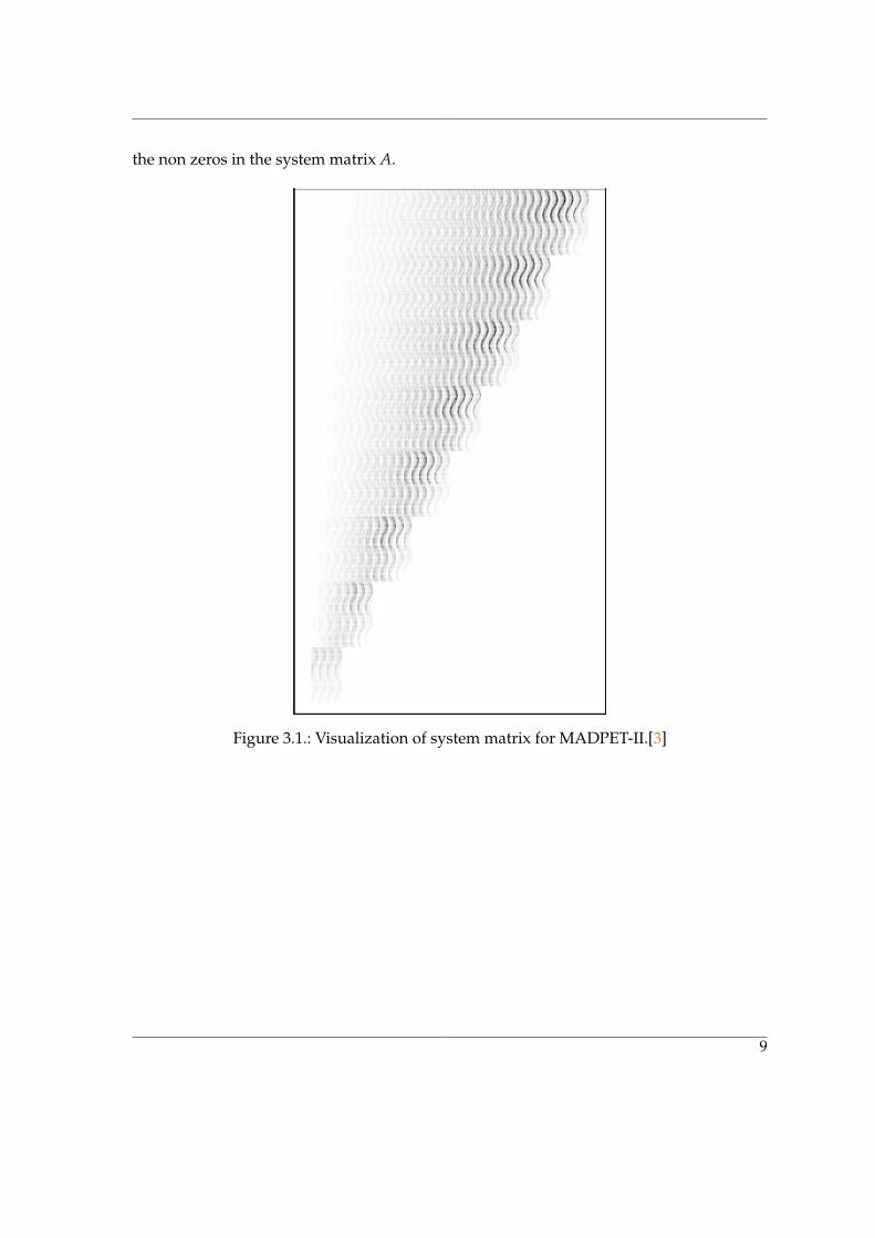
the non zeros in the system matrix A.

Figure 3.1.: Visualization of system matrix for MADPET-II.[33]

9

4. Sparse Matrix Format, SPMV and SPMV T

The system matrix A, with its 1327104 rows, 784000 columns and the sparsity of 0.1541%,if stored in a dense format the matrix would have required approximately 3800 gigabytes(with values stored as int and float) which would have been very difficult to handle. Thiswould have put a lot of unnecessary load on the I/O not to mention the memory andcomputational resource wastage.

As an example consider the addition of all the values of the matrix. If stored in the denseformat it would have required ≈ 1e12 operations instead of just ≈ 1.6e9 operations if onlythe non zeros are stored.

Due to the practical issues already mentioned, it becomes imperative that we consider”smart” formats for storing these really big matrices. So the format that has been usedto store the system matrix for the PET scanner MADPET-II is a sparse format called Com-pressed Sparse Row(CSR).

0 0 1 02 3 0 00 4 5 60 0 0 0

Table 4.1.: Full Matrix

CSR Rows (IA) 0 1 3 6 6

CSR Columns (JA) 2 0 1 1 2 3

CSR Value (A) 1 2 3 4 5 6

Table 4.2.: Matrix in CSR format

The table 4.14.1 shows a typical matrix stored in a dense format while the table 4.24.2 shows amatrix stored in the CSR format.

The CSR format is a row major format i.e left-to-right top-to-bottom. In this format thematrix is stored in three different one dimensional arrays. The CSR Rows in the table 4.24.2represents the number of non zeros in each row and it is of the size of number of rows + 1.[99]

The array CSR Columns stores the column number of each non zero element of thematrix and hence it is of the size equal to number of non zero elements in the matrix. TheCSR Value array stores all the non zero values of the matrix and hence its size is also sameas the size of CSR Columns i.e equal to number of non zero elements in the matrix.

10

4.1. Sparse Matrix Vector Multiplication(SPMV)

To access the values and columns associated with a row, first the number of non zerosin that row i are calculated by subtracting IA[i] from IA[i +1] i.e. (IA[i+1] - IA[i]). Nowthe columns where these non zeros exist and the values can be accessed starting from theindex number IA[i] in the CSR Columns and CSR Value arrays up-to the number of nonzeros in that particular row.

The two types of operation performed with the system matrix are Sparse Matrix VectorMultiplication(SPMV) and Transpose Sparse Matrix Vector Multiplication(SPMV T) and theother operations, like the calculation of norm 3.23.2 are derivative of these which will also betouched upon later.

4.1. Sparse Matrix Vector Multiplication(SPMV)

Sparse Matrix Vector Multiplication or SPMV, is the name given to a set of problems involv-ing the multiplication of a sparse matrix, CSR here, with a dense vector and hence thename. The memory and computational requirements are substantially reduced by the useof SPMV instead of dense matrix vector multiplication but the use has its own performancepitfalls, especially when using multicore systems.

Source code 4.14.1 shows a concise way to store the CSR matrix.

1 struct CSR_MATRIX{2 float num_rows;3 float num_columns;4 float nnz;5 std::vector<float> csr_vals;6 std::vector<int> csr_rows;7 std::vector<int> csr_cols;8 CSR_MATRIX(int nRows, int nColumns, int NNZ){9 num_rows = nRows;

10 num_columns = nColumns;11 nnz = NNZ;12 csr_vals.resize(nnz);13 csr_cols.resize(nnz);14 csr_rows.resize(nRows + 1);15 }16 };

Source Code 4.1.: A possible way to store matrix in Compressed Sparse Row (CSR) format.

11

4. Sparse Matrix Format, SPMV and SPMV T

1 CSR_MATRIX csr(nRows, nColumns, NNZ);2 std::vector vec(csr.num_columns);3 std::vector <float> spmv(csr.num_rows, 0);4 for (int i=0; i< csr.num_rows ; ++i)5 {6 int nnz_this_row = csr.csr_rows[i+1] - csr.csr_rows[i];7 for (int j =csr.csr_rows[i] ;8 j< csr.csr_rows[i] + nnz_this_row; ++j)9 {

10 int column_num = csr.csr_cols[j];11 spmv[i] += csr.csr_vals[j]*vec[column_num];12 }13 }

Source Code 4.2.: Sparse Matrix Vector Multiplication (SPMV)

The source code 4.24.2 shows how to perform SPMV with a matrix stored in CSR formatas shown in 4.14.1. The vec in 4.24.2 is the vector of size equal to number of columns of thematrix (csr.num columns) that has to be multiplied with the CSR matrix. For any row i, inline 6 we calculate the number of non zeros elements in the row and in line 7 we loop overthose number of elements starting from the element number stored at the ith place in thecsr rows array. Finally in line 9 we find out the column number of the value pointed toby the inner loop and subsequently multiply the value from the CSR values array and thecorresponding value from the vec array and add it into the output result(spmv array) ofrow i. The size of the generated output array is equal to the number of rows in the matrix.

4.2. Transpose Sparse Matrix Vector Multiplication(SPMV T)

The next system matrix operation is the multiplication of the transposed sparse matrixwith a vector. SPMV T could also be looked as the matrix stored in column major formatand then performing the SPMV over it. The problem with the second approach is that itis not always possible to store the matrix in row major and column major format side byside due to memory limitations. So it becomes very important that SPMV T operation isalso written in a way that the memory accesses are reduced to minimum.

The code 4.34.3 shows a possible way, for the matrix stored in CSR format(4.14.1), that istransposed and multiplied with a vector of size equal to number of rows of the matrix.The only change, apart from the changes in size of the input and output arrays in line 2-3,is that now the vector to be multiplied i.e. vec is accessed based on the row number and theresult is saved in the output array (line 10) corresponding to the column number instead of

12

4.2. Transpose Sparse Matrix Vector Multiplication(SPMV T)

the row number, as was the case in SPMV. The output array generated is of the size equalto the number of columns of the matrix.

1 CSR_MATRIX csr(nRows, nColumns, NNZ);2 std::vector vec(csr.num_rows);3 std::vector <float> spmv_t(csr.num_columns, 0);4 for (int i=0; i< csr.num_rows ; ++i)5 {6 int nnz_this_row = csr.csr_rows[i+1] - csr.csr_rows[i];7 for (int j =csr.csr_rows[i] ;8 j< csr.csr_rows[i] + nnz_this_row; ++j)9 {

10 int column_num = csr.csr_cols[j];11 spmv_t[column_num] += csr.csr_vals[j]*vec[i];12 }13 }

Source Code 4.3.: Transpose Sparse Matrix Vector Multiplication (SPMV T)

13

5. GPU Architecture and Programming

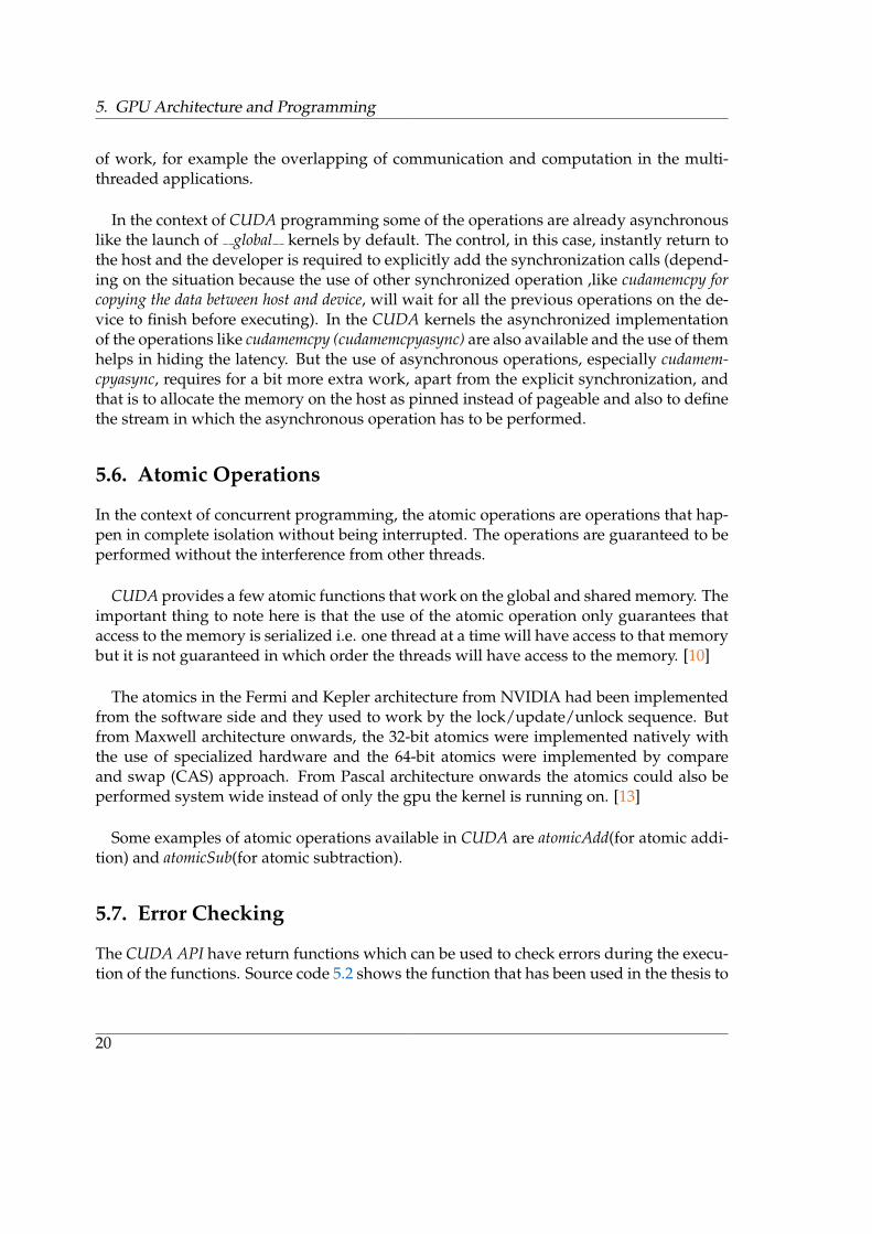
The Graphical Processing Units(GPU) were initially used to generate 2 or 3 dimensionalimages and videos that have to be outputted on the display device, be it operating systemor games. The need to design a new processing unit arised because the generation ofthe images require a high degree of data parallel computations, where there are lot morearithmetic operations compared to memory operations, and Central Processing Unit(CPU)with their very few cores, especially at the start of the century, were not ready to handle theworkload. This requirement finally lead to the development of devices which could handlehighly parallel compute intensive workloads where most of the transistors are devoted tothe data processing instead of data caching and flow control where CPU has the lead.[1010, 1111]

Figure 5.1.: Central Processing Unit (CPU) vs Graphical Processing Unit (GPU)[1010](NOTE:Not to scale.)

The Figure 5.15.1 shows how the area on a CPU and GPU die is split into different com-ponents. In the CPU a lot of die area (percentage wise) is used for cache and control logicwhereas in the case of GPU most of the area (percentage wise) is used for compute units.This is the reason why the CPU manufactures like Intel could add a lot of new instructionsets (AVX, SSE, MMX etc). The CPU’s could also run at a much better clock frequency andare far ahead of GPUs in speculative execution, branch prediction, and store forwarding.[1212]

Even when the GPUs were only used for the graphical applications and there was noeasy way to communicate or program the device for the non graphics developers, it did notdeter few brave souls, who understood the power of the GPUs to try to use them for their

14

5.1. Grids, Blocks and Threads

application using the graphics APIs like Direct3D and OpenGL. Due to these limitations thelearning curve was steep and the full potential of the GPUs could not be utilized.

This all changed with the release of Compute Unified Device Architecture (CUDA) for GPUsby NVIDIA in 2007. For the first time the non graphical developers had an API that en-abled them to use GPU for general purpose processing. It provided them a software layerthat gives access to the GPU’s virtual instruction set and parallel compute units, for the ex-ecutions of compute kernels. The CUDA was designed to work with the languages C, C++and FORTRAN but now it could also be used from other languages like Java and Pythondue to the wide availability of wrappers.

The CUDA programming model was designed to allow developers to leverage the mul-tiple cores in the GPU to develop transparently scalable software without the hassle oflearning the graphical programming as was the case before. CUDA provided three ab-stractions at its core; hierarchy of thread groups, shared memories, and barrier synchro-nization. These abstractions allowed the developer to partition the problem into coarsesub problems that can be solved simultaneously and independently by a group of threadsin a block where the threads could solve it cooperatively by breaking the sub problem intoeven finer pieces. [1010]

The chapter tries to give an overview to the architecture of the CUDA capable NVIDIAGPUs, the programming model along with a few optimization techniques that could ac-celerate the performance of the SPMV and SPMV T operations.

5.1. Grids, Blocks and Threads

The threads in a CUDA kernel can be arranged in 1D, 2D or 3D and subsequently arecalled one, two or three dimensional thread block respectively. This idea is very helpful asit helps in mapping a vector, matrix or volume domain logically across the threads. But itshould be kept in mind here that the number of threads in a thread block could not exceed1024 as all the threads are supposed to reside on the same streaming multiprocessor andare expected to share the limited resources of that streaming multiprocessor. So some ofthe possible configurations for the thread block could be (1024,1,1) or (16,8,8).

The blocks are further arranged in 1D, 2D or 3D and subsequently are called one, twoor three dimensional block grid respectively. The grid size can far exceed the number ofavailable thread blocks that a GPU can process simultaneously as it is dependent on thesize of data being processed.

Since the dimension of the thread block and block grid could be 2D and 3D apart fromlinear (which could be handled with data type int also), NVIDIA has introduced a new

15


data type called dim3. The possible example for the 1D block is (1024,1,1) for 2D is (32,32,1)and for 3D is (16,8,8). Now to calculate the global thread index of a thread, CUDA providesaccess to three variables called blockIdx, blockDim and threadIdx. With the help of variableblockIdx the index of a block could be calculated locally in a grid like blockIdx.x for thefirst dimension and so on. The variable blockDim tells the size of the grid like blockDim.xfor the first dimension of the block and so on. And finally the variable threadIdx tells theuser about the local thread number in a block. Using these three variables the global indexof the thread could be calculated as shown in 5.15.1 for a 2D grid and 2D block.

1 int i = blockIdx.x * blockDim.x + threadIdx.x;2 int j = blockIdx.y * blockDim.y + threadIdx.y;

Source Code 5.1.: Calculating local thread id in a 2D thread block in a 2D block grid.

Figure 5.2.: Grid of Thread Blocks[1010]

The figure 5.25.2 gives a visual representation of the nesting of a 2D block in a 2D gridwhere the size of block grid is (3,2,1) while the size of thread block is (4,3,1).

16

5.2. Register, Local, Constant, Shared, Global, and Texture memory

5.2. Register, Local, Constant, Shared, Global, and Texturememory

CUDA capable devices have a memory hierarchy where each type of memory has its ad-vantages and disadvantages and selecting the correct memory to save the data could havesignificant effect on the performance of the kernels.

• Register: The fastest of all the memories but it is only accessible by the thread andhas the lifetime of the thread.

• Local: This is not a physical type of memory but an abstraction of global memory. Ithas the same scope as registers. Since this memory resides off chip, the access to it isvery slow and it is only used in the case when registers are out of space.

• Constant: This memory is accessible by all threads but is read only. It has the lifetimeof an application.

• Shared: This memory has the lifetime of a block and let the threads in a block sharedata among themselves. It is also a fast memory only when there are no bank con-flicts.

• Global: This memory is the largest and the slowest at the same time. It has thelifetime of an application and is accessible by all the threads in the application.

• Texture: This is another type of read only memory which is accessible by all threadsin the application. This memory is really helpful in applications where there is a lotof spatial locality.

The figure 5.35.3 shows the different type of memory which reside on the GPU. Apart fromthat it also tells that the global, constant and texture memory are the only ones accessiblefrom the host.

The table 5.15.1 lists the amount of different types of memory available in NVIDIA TeslaP100 (NVIDIA Pascal Architecture based GPU in DGX-1).

17


Memory Type SizeGlobal 16 GB

Register/SM 256 KBRegister/GPU 14336 KB

Shared/SM 64 KBShared/GPU 3584 KB

Constant 65536 BytesTexture As large as Global

Table 5.1.: Different memory size in NVIDIA Tesla P100[1313]

Figure 5.3.: Memory Hierarchy on GPU [1414]

18

5.3. Host, Device and Global Kernels

5.3. Host, Device and Global Kernels

These are the function space execution specifiers which tell the compiler which functionhas to be executed on the device and which on host apart form whether it is callable fromdevice or from host.

• device : This execution space identifier declares that the function is to be executedon the device i.e. GPU and will be callable from the device only.

• host : This execution space identifier declares that the function is to be executedon the host and is only callable from the host. If the specifier is omitted then thecompiler assumes that the function has to compiled for the host i.e. CPU.

• global : This execution space identifier declares that the function is to be executedon the device and will be callable from the host and from the device (With CUDAcapable devices having compute capability higher than 3.2). A global functionmust have a void return type and cannot be a member of class. Moreover the call toa global function is asynchronous.

These specifiers could also be used together but all the combinations are not possible.For example the global / device and global / host specifiers could not be used to-gether while the device / host can be.[1010]

5.4. Streams and Events

The CUDA stream represent a sequence of operations which are executed in the orderthey are issued. The steams are the work queues to express concurrency between differenttasks. The streams are particularly helpful to make use of the GPU fully. For example,on one stream a kernel execution could be launched while on the other stream memorytransfer from host to device and from device to host could be performed(this will alsodepend on the available resources: two copy engines, compute resources).

CUDA events are synchronization markers that are used to synchronize the tasks fromdifferent streams, allow fine grained synchronization within a stream and finally to allowinter leave synchronization.

5.5. Asynchronous Kernels and Copy Operations

Asynchronous operations are those which does not block the process for the finishing ofthe operation. They do not wait for the return value and hence it is the job of the developerto make sure that the operation has completed before using the result. Now these opera-tions, although requiring more work, are very helpful in overlapping two different kind

19


of work, for example the overlapping of communication and computation in the multi-threaded applications.

In the context of CUDA programming some of the operations are already asynchronouslike the launch of global kernels by default. The control, in this case, instantly return tothe host and the developer is required to explicitly add the synchronization calls (depend-ing on the situation because the use of other synchronized operation ,like cudamemcpy forcopying the data between host and device, will wait for all the previous operations on the de-vice to finish before executing). In the CUDA kernels the asynchronized implementationof the operations like cudamemcpy (cudamemcpyasync) are also available and the use of themhelps in hiding the latency. But the use of asynchronous operations, especially cudamem-cpyasync, requires for a bit more extra work, apart from the explicit synchronization, andthat is to allocate the memory on the host as pinned instead of pageable and also to definethe stream in which the asynchronous operation has to be performed.

5.6. Atomic Operations

In the context of concurrent programming, the atomic operations are operations that hap-pen in complete isolation without being interrupted. The operations are guaranteed to beperformed without the interference from other threads.

CUDA provides a few atomic functions that work on the global and shared memory. Theimportant thing to note here is that the use of the atomic operation only guarantees thataccess to the memory is serialized i.e. one thread at a time will have access to that memorybut it is not guaranteed in which order the threads will have access to the memory. [1010]

The atomics in the Fermi and Kepler architecture from NVIDIA had been implementedfrom the software side and they used to work by the lock/update/unlock sequence. Butfrom Maxwell architecture onwards, the 32-bit atomics were implemented natively withthe use of specialized hardware and the 64-bit atomics were implemented by compareand swap (CAS) approach. From Pascal architecture onwards the atomics could also beperformed system wide instead of only the gpu the kernel is running on. [1313]

Some examples of atomic operations available in CUDA are atomicAdd(for atomic addi-tion) and atomicSub(for atomic subtraction).

5.7. Error Checking

The CUDA API have return functions which can be used to check errors during the execu-tion of the functions. Source code 5.25.2 shows the function that has been used in the thesis to

20

5.8. Coalesced Memory Access

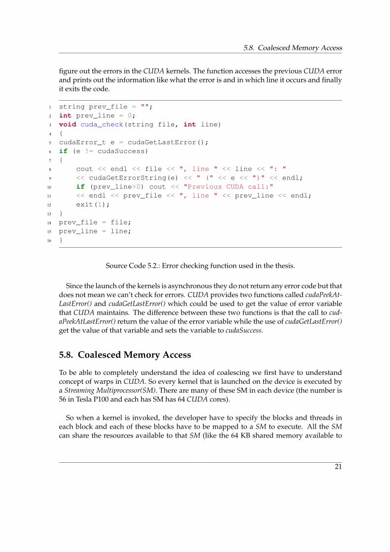
figure out the errors in the CUDA kernels. The function accesses the previous CUDA errorand prints out the information like what the error is and in which line it occurs and finallyit exits the code.

1 string prev_file = "";2 int prev_line = 0;3 void cuda_check(string file, int line)4 {5 cudaError_t e = cudaGetLastError();6 if (e != cudaSuccess)7 {8 cout << endl << file << ", line " << line << ": "9 << cudaGetErrorString(e) << " (" << e << ")" << endl;

10 if (prev_line>0) cout << "Previous CUDA call:"11 << endl << prev_file << ", line " << prev_line << endl;12 exit(1);13 }14 prev_file = file;15 prev_line = line;16 }

Source Code 5.2.: Error checking function used in the thesis.

Since the launch of the kernels is asynchronous they do not return any error code but thatdoes not mean we can’t check for errors. CUDA provides two functions called cudaPeekAt-LastError() and cudaGetLastError() which could be used to get the value of error variablethat CUDA maintains. The difference between these two functions is that the call to cud-aPeekAtLastError() return the value of the error variable while the use of cudaGetLastError()get the value of that variable and sets the variable to cudaSuccess.

5.8. Coalesced Memory Access

To be able to completely understand the idea of coalescing we first have to understandconcept of warps in CUDA. So every kernel that is launched on the device is executed bya Streaming Multiprocessor(SM). There are many of these SM in each device (the number is56 in Tesla P100 and each has SM has 64 CUDA cores).

So when a kernel is invoked, the developer have to specify the blocks and threads ineach block and each of these blocks have to be mapped to a SM to execute. All the SMcan share the resources available to that SM (like the 64 KB shared memory available to

21


each SM in Tesla P100 ). But the SM tries to further divide the block internally so that eachthread share the same code and follow the same execution path with minimal divergenceand stall at the same point in the kernel. The thread group generated because of this furthersplitting by the SM is called a warp and the current maximum size of it is 32 threads forNVIDIA GPUs.

There are definitely some disadvantages of this approach also especially when differentthreads take different execution path which leads to the under-utilization of the hardwareresources.

The global memory in the device is accessed via 32,64 or 128 byte memory transactions.Now if these memory are aligned perfectly with the size of the warp and warps execute aglobal memory access instruction, it tries to coalesce into as less memory transactions aspossible because every global memory access instruction induces a penalty on the through-put of the device. So for example suppose that each thread in a warp (32 threads) has toaccess a float value (4 bytes) in the global memory and if the memory access is coalescedand the memory is contiguous then this transaction will be completed in a single step butit could go as bad as 32 transactions in the worst case. [1515]

1 __global__ void mat_vec_mul( float* result,2 const float* vec,3 const float* csrVal_d,4 const int* csrRowInd_d,5 const int* csrColInd_d,6 const uint32_t rows)7 {8 uint32_t i = threadIdx.x + blockIdx.x*blockDim.x;9

10 if (i<rows){11 uint32_t col_num;12 for (uint32_t j=csrRowInd_d[i]; j< csrRowInd_d[i+1] ; ++j){13 col_num = csrColInd_d[j];14 result[i] += vec[col_num]*csrVal_d[j];15 }16 }17 }

Source Code 5.3.: Example of a non coalesced global memory access in SPMV kernel.

22

5.9. Pinned Memory

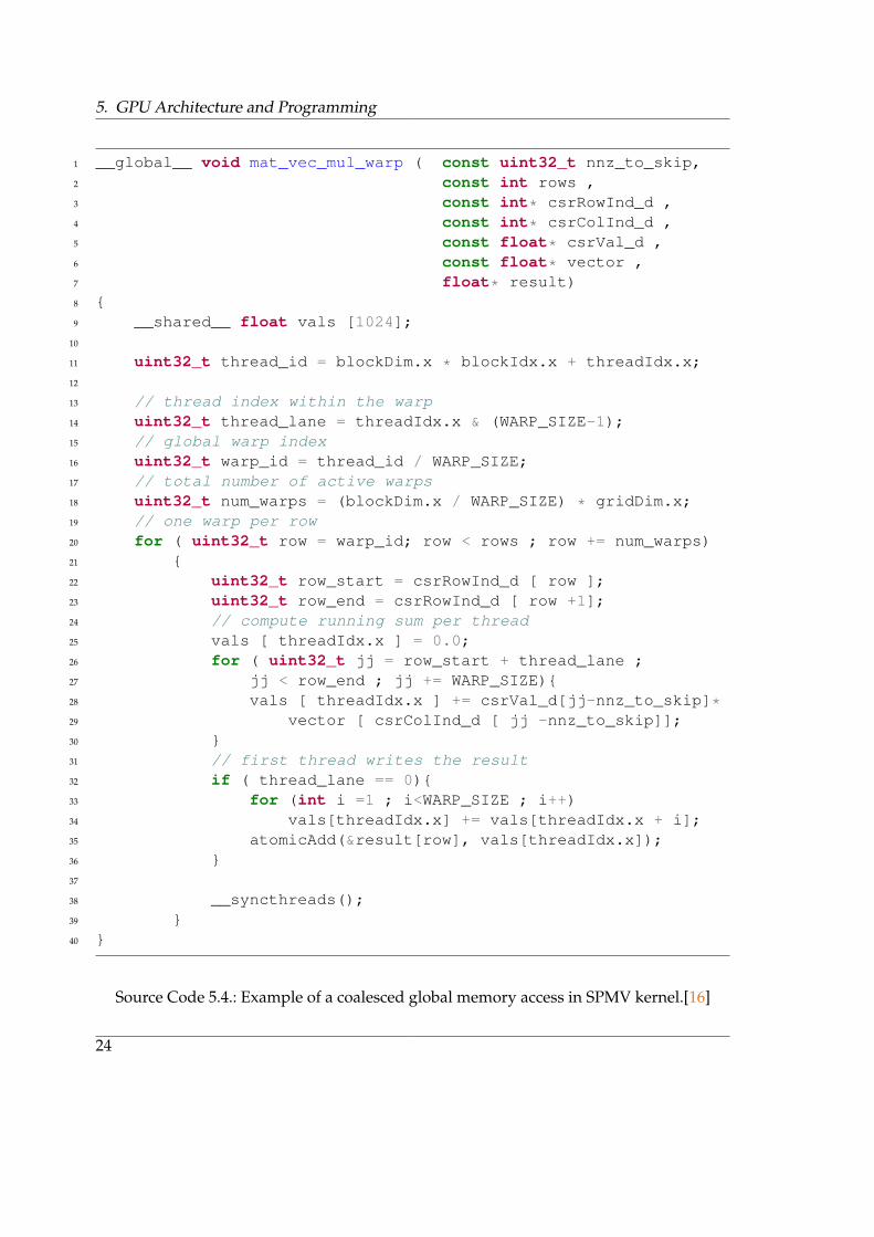
The code 5.35.3 shows an example where the coalescing of the global memory access is notimplemented in the SPMV kernel and the code 5.45.4 shows the example when it is imple-mented. The performance of these two kernels have been compared in the Part II of thethesis.

5.9. Pinned Memory

The memory is called pinned because after being allocated it could not be swapped outfrom the system memory, for example to the swap partition on the hard drive. In otherwords once it is given a place in the host memory then it could not be evicted. This type ofallocation leads to improved I/O efficiency but on the other side the allocation of the pinnedmemory takes a bit more time compared to the pageable memory. Moreover the allocationof too much pinned memory actually degrades the performance of the code so it shouldbe used with care. [1717]

In CUDA the pinned memory on the host could be allocated with the help of two func-tions namely, cudaHostAlloc() and cudaHostMalloc(). These two functions doesn’t have anydifference when cudaHostAlloc() is used in the default mode.

The final implementation is using the pinned memory because of the inherent compul-sion to use it when using asynchronous functions in the multi GPU case. The pinned mem-ory is further allocated with the option cudaHostAllocPortable because then the memory isconsidered pinned for all the contexts and not just the current context.

5.10. Bank Conflicts

Shared memory is a type of on-chip memory and hence it has much lower latency andmuch higher bandwidth. To achieve even better bandwidth the shared memory avail-able per block is divided into multiple equally size memory modules called banks (thereare 32 banks in the modern SM which is equal to the warp size). The memory accessesby the threads to these different banks could be handled at the same time (and thus thebandwidth increases by the factor equal to number of simultaneous memory requests) butthe bank conflicts occur when more than 1 thread tries to access the same memory bank.The hardware handles this by splitting the requests into as many conflict free requests aspossible which is ultimately responsible for bandwidth penalty. [1818, 1919]

23


1 __global__ void mat_vec_mul_warp ( const uint32_t nnz_to_skip,2 const int rows ,3 const int* csrRowInd_d ,4 const int* csrColInd_d ,5 const float* csrVal_d ,6 const float* vector ,7 float* result)8 {9 __shared__ float vals [1024];

10

11 uint32_t thread_id = blockDim.x * blockIdx.x + threadIdx.x;12

13 // thread index within the warp14 uint32_t thread_lane = threadIdx.x & (WARP_SIZE-1);15 // global warp index16 uint32_t warp_id = thread_id / WARP_SIZE;17 // total number of active warps18 uint32_t num_warps = (blockDim.x / WARP_SIZE) * gridDim.x;19 // one warp per row20 for ( uint32_t row = warp_id; row < rows ; row += num_warps)21 {22 uint32_t row_start = csrRowInd_d [ row ];23 uint32_t row_end = csrRowInd_d [ row +1];24 // compute running sum per thread25 vals [ threadIdx.x ] = 0.0;26 for ( uint32_t jj = row_start + thread_lane ;27 jj < row_end ; jj += WARP_SIZE){28 vals [ threadIdx.x ] += csrVal_d[jj-nnz_to_skip]*29 vector [ csrColInd_d [ jj -nnz_to_skip]];30 }31 // first thread writes the result32 if ( thread_lane == 0){33 for (int i =1 ; i<WARP_SIZE ; i++)34 vals[threadIdx.x] += vals[threadIdx.x + i];35 atomicAdd(&result[row], vals[threadIdx.x]);36 }37

38 __syncthreads();39 }40 }

Source Code 5.4.: Example of a coalesced global memory access in SPMV kernel.[1616]

24

6. Other Terminologies

There are three more terminologies that have been used in the thesis and thus they warranta brief introduction and this chapter is about those three terms.

6.1. Heterogeneous Computing

Heterogeneous Computing refers to the systems in which there are more than one kind ofprocessors working together to solve a task and each one of them is specialized for certainkind of tasks. An example of that is the use of GPU along with the CPU to solve a problemas is the case in the present thesis. This approach can be scaled further to create a networkof these heterogeneous systems where there could be one or more co-processors i.e GPUconnected to a single host. The MAC cluster in LRZ is based on this very same idea.

In heterogeneous computing it is not always necessary that the host and the co-processorsare all of the same type and this introduces additional difficulties in workload balancing.

The thesis is an attempt to harness the power of the host and co-processor in the bestpossible way to solve the MLEM algorithm as fast as possible especially when there is notenough memory on the GPU to store the entire matrix at once

6.2. CUDA Aware MPI

MPI stands for Message Passing Interface and it is a communication protocol for communi-cating data between distributed processes through messages. It is written with scalabilityfor multi node systems in mind. Now the non cuda aware MPI implementation could beused easily to communicate data in the multi core heterogeneous systems but it involvesa bit of extra work to achieve that and also leads to performance hit. Due to the abovementioned reasons it is a good idea to combine the parallel programming approaches ofCUDA and MPI.

To start a multi core distributed code, MPI requires that the user provides the numberof processes the application should scale to. Now to exchange data between the processes(where some calculation has been performed by the GPU), in the non cuda aware mode thedata from the GPU has to be copied back for the host to send and when the host receives thedata then that has to be again copied into the GPU explicitly. Now this approach requires

25


4 commands to achieve instead of just 2, if we use the cuda aware MPI. The example 6.16.1 and6.26.2 shows this difference.

1 //on MPI rank 02 cudaMemcpy(h_send_buf, d_send_buf, size, cudaMemcpyDeviceToHost);3 MPI_Send(h_send_buf, size, MPI_FLOAT, 1, 0, MPI_COMM_WORLD);4

5 //on MPI rank 16 MPI_Recv(h_recv_buf, size, MPI_FLOAT, 0, 0, MPI_COMM_WORLD,&stat);7 cudaMemcpy(d_recv_buf, h_recv_buf, size, cudaMemcpyHostToDevice );

Source Code 6.1.: Example of communication between processes when the MPI is notCUDA aware.

1 //on MPI rank 02 MPI_Send(d_send_buf, size, MPI_FLOAT, 1, 0, MPI_COMM_WORLD);3

4 //on MPI rank 15 MPI_Recv(d_recv_buf, size, MPI_FLOAT, 0, 0, MPI_COMM_WORLD,&stat);

Source Code 6.2.: Example of communication between processes when the MPI is CUDAaware.

The feature works because of the Unified Virtual Addressing(UVA) introduces with CUDA4.0 (for GPU from Fermi architecture onwards). The UVA allows the memory of host andall the devices connected to it in a system, to be treated as a single virtual address space. Inthe absence of UVA, the MPI would have to be told where the memory lives i.e on host oron device, which could have been achieved automatically or with an addition argument inthe MPI commands. The figure 6.16.1 shows how the UVA maps all the memory in a systemto a single virtual address space. [2020]

The use of CUDA aware MPI accelerates the communication by pipelining all the opera-tion in the message transfer and also by the use of acceleration technologies like GPUDirectimplemented incrementally by NVIDIA from Kepler architecture onwards. An exampleof the GPUDirect technology, figure 6.26.2, is the GPUDirect P2P, which is used to transferthe memory from one GPU to another without being staged through the host during intranode communication. This approach leads to a higher bandwidth and low latency com-munication between GPUs.

26

6.3. Floating Point Arithmetic

Figure 6.1.: Mapping of memory in a system with UVA(right) and without UVA(left)[2020]

Figure 6.2.: The communication without the use of GPUDirect P2P (left) and with GPUDi-rect P2P (right)[2020]

Even in the GPUs with Fermi architecture, which do not have any of the GPUDirecttechnologies implemented, the use of CUDA Aware MPI leads to faster communicationdue to the fact that is pipelines the communication and reduces some bottlenecks.


This section will try to give a very brief overview of the what floating point numbers are,how they are represented into the computers, IEEE-754 standards and finally the differ-ence between results that are encountered during the course of the thesis and the possiblereasons for those differences.

The floating point numbers are called so because in these numbers the binary/decimalpoint can float over the significant digits based on the exponent. For example the 1.2345with its 5 significant digits can be represented as 1.2345x100 or as 12345x10-4.

The representation 1.2345x100 is also called the normalized scientific notation. In the nor-malized scientific notation a floating number is represented as d0.d1d2d3...dn-1 x βe. In thisrepresentation d0.d1d2d3...dn-1 are called the n significant digits, β the base and e the ex-ponent. In this representation it is also required that the absolute value of d0.d1d2d3...dn-1

27


should be greater than 1 and less than 10 (for the representation in base 10). [2121]

The modern day computers are made up of billions of transistors and those transistorshave only 2 states i.e 0 and 1. This is the reason why the floating point numbers in the com-puters are represented in base 2. Although it is possible to simulate the decimal numberswith binary circuits as well but it leads to less efficient implementation.

The need to have a floating point standard like IEEE-754 arised because in the earlierdays of computer era the vendors were implementing floating point arithmetic in theirown way. For example IBM was using some guard digits to perform the floating pointarithmetic exactly and then rounding of the result. This lead to the situation where pro-grams were not giving same result on different machines which in some applications couldhave cascading effects. The IEEE-754 standard released in the year 1985 was an attempt tosolve this reliability and portability problem by laying down the rules for representation offloating point numbers, their interchangeability, rounding errors, exception handling andoperations. [2222]

The floating point number in the IEEE-754 is represented by 32 bits in base 2. The 32bits are divided into 3 parts. The first 23 bits are allocated for the significant digits, thenext 8 are saved for the exponent and the last one for the sign of the number. With thisrepresentation the values in the range≈ -1.4e-38 to≈ 3.4e38 could be stored as floating pointnumbers. [2323]

Out of the four basic arithmetic operations, addition, subtraction, multiplication anddivision, the use of addition and subtraction in the case where one number is very largeand another one require special attention. The reason for that is that the while addingor subtraction floating point numbers, IEEE-754 require that the exponents are matchedand then the fraction part is added up. Now this operation has the unintended effect ofthe dropping out of the smaller of the two completely (in the worst case) because of thelimited number of available bits to save the fraction part.

For example, the summation of 1.0e0 and 1.0e-8 in 32 bits would give an output of 1.0e0

which is not correct if looked from the perspective of exact arithmetic. The table 3.13.1 showsthat the values in the system matrix are also quite far apart and hence these kind of errorscould also crept there and they did. The interesting thing to note here is that even the resultfrom the CPU and the GPU, when both use IEEE-754 standards, were slightly different,7108.830078 vs 7109.272461 when taking the sum of all the non zero values in the matrix.

28


1 #ifndef __STDC_IEC_559__2 #error "Requires IEEE 754 floating point!"3 #endif4

5 #include <iostream>6 #include <cblas.h>7 #include <cublas_v2.h>8 #include <cuda_runtime.h>9

10 int main(int argc, char *argv[]){11 size_t array_size = 1e8 + 1;12 float *array = (float*) malloc(array_size*sizeof(float));13 array[0] = 1;14

15 float seq_sum = 0.0;16 for (int i=0; i<array_size ; ++i) seq_sum += array[i];17

18 float cpu_blas_sum = 0;19 cpu_blas_sum = cblas_sasum(array_size, array, 1);20

21 cublasHandle_t cublasHandle;22 cublasCreate(&cublasHandle);23 float* array_d;24 cudaMalloc((void**)&array_d , array_size*sizeof(float));25 cudaMemcpy(array_d , array , array_size*sizeof(float),26 cudaMemcpyHostToDevice);27

28 float gpu_blas_sum = 0.0;29 cublasSasum(cublasHandle, array_size, array_d, 1,30 &gpu_blas_sum);31

32 delete [] array;33 cublasDestroy(cublasHandle);34 cudaFree(array_d);35

36 std::cout << "seq_sum:" << seq_sum << std::endl;37 std::cout << "cpu_blas_sum:" << cpu_blas_sum << std::endl;38 std::cout << "gpu_blas_sum:" << gpu_blas_sum << std::endl;39 return 0;}

Source Code 6.3.: Code to study the effect of summing up an array using different meth-ods.

29


1 seq_sum: 12 cpu_blas_sum: 1.753 gpu_blas_sum: 1.99968

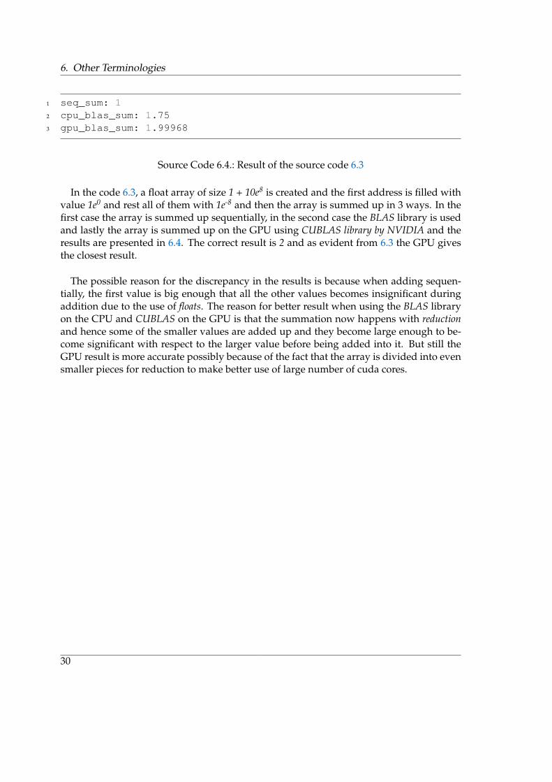
Source Code 6.4.: Result of the source code 6.36.3

In the code 6.36.3, a float array of size 1 + 10e8 is created and the first address is filled withvalue 1e0 and rest all of them with 1e-8 and then the array is summed up in 3 ways. In thefirst case the array is summed up sequentially, in the second case the BLAS library is usedand lastly the array is summed up on the GPU using CUBLAS library by NVIDIA and theresults are presented in 6.46.4. The correct result is 2 and as evident from 6.36.3 the GPU givesthe closest result.

The possible reason for the discrepancy in the results is because when adding sequen-tially, the first value is big enough that all the other values becomes insignificant duringaddition due to the use of floats. The reason for better result when using the BLAS libraryon the CPU and CUBLAS on the GPU is that the summation now happens with reductionand hence some of the smaller values are added up and they become large enough to be-come significant with respect to the larger value before being added into it. But still theGPU result is more accurate possibly because of the fact that the array is divided into evensmaller pieces for reduction to make better use of large number of cuda cores.

30

Part II.

Experiments and Results

31

7. Benchmarking MAC Cluster

The purpose of doing this test was two-fold. One, to gauge the performance of FermiArchitecture based GPUs (M2090) in Mac cluster vs Pascal Architecture based GPUs availablein DGX-1. Secondly, the default MPI implementation available in Mac Cluster is from Inteland so it was also interesting to see how other implementations perform on it. So, theother MPI implementation used is OpenMPI.

For this test all the 4 nodes (2 sockets per node) available in the cluster were used. Only1 task per socket was launched and the processes were bound to the core. For each MPIimplementation the application was launched 50 times and in each run 10 iterations wereperformed.

The figure 7.1a7.1a and 7.1b7.1b shows that the GPUs are solving the SPMV and SPMV T op-eration at almost the same speed across processes. The slight variation in performancecould be explained by the fact that the matrix is divided between the processes equallywith respect to non zero values. Now in the figure 3.13.1 it could be seen that the non zerosare more in initial rows and they subsequently decrease in later rows. So this leads to thecase where the initial ranks have more non zeros per row and later ranks have more rowsfor same number of non zeros.

The ”U” shape created by the later ranks in figure 7.1a7.1a could be probably because whenthe non zeros per row falls, it leads to less computation per thread and the device has tolaunch more thread blocks which brings with it some overhead.

The ≈ 28ms it takes to perform the Forward Projection on the Mac Cluster is 7 timesslower than the time it takes to perform the same operation on DGX-1 (Chapter 1010). Thethings gets even more interesting, 64.6 ms vs 7.3 ms, in the case of Backward Projection.Here the speedup is almost 8.9 times and this effect could be explained by the presence ofhardware support for atomics in the Pascal Architecture based GPUs which was absent in Fermibased GPUs (Backward projection uses lot more atomics compared to Forward Projection).

The figures 7.1c7.1c and 7.1d7.1d presents the time it takes to perform the reduction operation atdifferent stages in the application. After the norm calculation, the MPI Allreduce operationis performed for the first time and here the OpenMPI takes a lot more time compared tothe Intel MPI but once that is over and when again the reduction operations are performedduring the iterations, the OpenMPI edges slightly ahead of the Intel MPI.

32

(a) Time to perform Forward Projection(SPMV).

(b) Time to perform Backward Projec-tion (SPMV T).

(c) Time taken to reduce the norm cal-culated.

(d) Time taken to perform reduction inthe loop.

Figure 7.1.: Mac cluster benchmarking results.33

8. Effect of Cuda Aware MPI, PinnedMemory and Custom Kernels

The final MLEM implementation was not achieved in a single attempt. There were few it-erations where different path to achieve a objective was implemented, studied and finallythe best possible was chosen. This chapter show the effect of some of those implementa-tions on the performance on different kernels.

The table 8.18.1 shows the difference between different implementations. For example inthe version 1,2 and 3 the only difference is whether the reduction is implemented withor without CUDA AWARE MPI and if not then whether the memory for it was pinned ornot. The differences between version 5 and 6 are that the version 6 is not CUDA AWAREand it uses pinned memory for the reduction, it is also the only one which allocated pinnedmemory for the CSR arrays and finally the last difference is between the block size used forthe SPMV and SPMV T kernels. The block size in the case of the version 5 is 1024 and inthe case of version 6 it is 64.

Change\Versions V 1 V 2 V 3 V 4 V 5 (1024) V 6 (64)Cuda Aware NO NO YES YES YES NO

Pinned Mem for Reduction NO YES N/A N/A N/A YESPinned Mem for CSR NO NO NO NO NO YES

CuSparse SPMV YES YES YES NO NO NOCuSparse SPMV T YES YES YES NO NO NO

Coalesced Mem Access SPMV T NO NO NO NO YES YESNon Coalesced Mem Access SPMV T NO NO NO YES NO NO

Coalesced Mem Access SPMV NO NO NO NO YES YESNon Coalesced Mem Access SPMV NO NO NO YES NO NO

Table 8.1.: Differences between implementations.

The test was performed on the DGX-1 with 8 MPI processes. Each MPI processes wasallocated a GPU and the MPI processes were bound to core. The data for each version wascollected by running it 20 times and each time 10 iterations were performed.

The figure 8.1a8.1a tells that it takes a considerably less time to load the data and convert it

34

(a) Loading and converting the datainto CSR format.

(b) Allocation of memory on the deviceand copying the data into it.

(c) Performance of SPMV kernel in dif-ferent implementations.

(d) Performance of SPMV T kernel indifferent implementations.

Figure 8.1.: Performance difference between implementations.35

8. Effect of Cuda Aware MPI, Pinned Memory and Custom Kernels

into the CSR format, if pinned memory is used for it. The possible reasons for the widevariations between the timing for the same version are the I/O limitations because all theprocesses will try to read the data at the same time and so some will read it faster thanthe others. The other reason for the variation could be from how the experiment wasperformed. For performing the experiment the MPI processes were bound to the core butthey were free to be allocated on any core of the dual socket DGX-1.

The figure 8.1b8.1b shows that the time to send the data to the GPU is much faster if thepinned memory is used and the variation between the timing is also very less in that case.

The forward projection time in different implementations, figure 8.1c8.1c, shows that thecustom SPMV implementation using coalesced memory access and the Cusparse imple-mentation provided by NVIDIA are very close in terms of performance but the same can’tbe said about the non coalesced version implemented in the case of version 4. Moreover,there is not much variation between timing in the implementations, apart from non coa-lesced memory access version, and the reason for that is due to the non zeros in the rowsthat are allocated to each MPI process.

The backward projection time for different implementations is shown in figure 8.1d8.1d. Itshows the custom kernel written using coalesced memory access is faster than the SPMV Timplementation provided by NVIDIA. The possible reason for this behaviour could be thatthe kernels provided by NVIDIA are guaranteed to provide bit wise same result and thereis no efficient way to achieve that yet in SPMV T. Here again the performance hit becauseof not using coalesced memory could be seen in version 4.

The figure 8.28.2 shows the time it takes to perform reduction operation reduces whenpinned memory is used but it increases when the CUDA AWARE MPI is used. The possi-ble reason could be because of the fact that the MPI was not built considering the under-lying communication network which might degrade the performance. But still it warrantsfurther scrutiny. The reason for the variation between processes stems from the SPMV Tcalculation difference from earlier in the iteration loop, figure 8.1d8.1d, and hence they shouldbe viewed together. The process which finishes the Backward Propagation faster has towait longer at the reduction step.

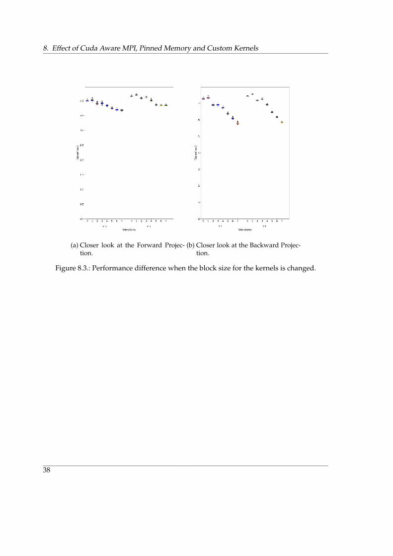
The figures 8.3a8.3a and 8.3b8.3b provides a closer look at the performance difference whenthe block size for the kernels is changed from (1024,1,1) in implementation 5 to (64,1,1) inimplementation 6. It could be seen that unexpectedly there is a performance hit going fromversion 5 to version 6. It was expected that the performance will improve with this changeas the kernel allocates a warp to a row and so when the row is big it stalls the entire blockand going for a smaller block was supposed to alleviate this and improve performance.

36

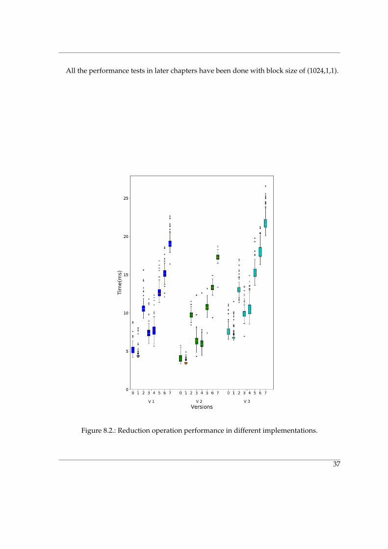
All the performance tests in later chapters have been done with block size of (1024,1,1).

Figure 8.2.: Reduction operation performance in different implementations.

37

8. Effect of Cuda Aware MPI, Pinned Memory and Custom Kernels

(a) Closer look at the Forward Projec-tion.

(b) Closer look at the Backward Projec-tion.

Figure 8.3.: Performance difference when the block size for the kernels is changed.

38

9. Effect of Splitting Work between CPU andGPU

This test was performed to see the effect of how the problem scales when more and morepart is solved on the GPU. For this test the DGX-1 machine was used and the applicationwas launched with only 1 MPI process. The application was bound to the core and themapping was done per core. For solving the part on the CPU this application uses 2 Openmpthreads, which are on the same core. The tests were performed 50 times with 10 iterationsfor each distribution of work between host and device.

(a) Time to calculate initial value andthen initializing image vector.

(b) Total time for Allocation and Initial-ization Operations.

Figure 9.1.: Time to perform Allocation and Initialization Operations.

The figure 9.1a9.1a shows the difference between the time it takes for initializing the image

39

9. Effect of Splitting Work between CPU and GPU

vector of size 784,000 floats on the CPU and on the GPU. Before initialization of the image,the initial value is calculated by performing 2 BLAS operation on the GPU. The drasticdrop when only using GPU is because now there is no need for a Image vector on the host.It is also important to note here the image initialization on the host is also accelerated byOpenMP.

In the figure 9.1b9.1b the effect of the increasing workload allocation to the device withrespect to the total allocating and initializing vectors time could be seen. The Norm Calcu-lation, SPMV T operation where the vector is a unit vector, time reduces as we increase thepercentage allocation on the device which is exactly what is expected.

(a) Time to calculate correlation. (b) Time to reduce Backward Proj.

Figure 9.2.: Effect of increasing device workload on Correlation calculation andMPI Allreduce time.

After partitioning the system matrix, the application has to determine which part has tobe solved on the host and which on the device and this splitting is performed in FurtherPartition. Again the constant partition time is what is expected from the application.

As more and more part is allocated to the device, more of the initial data has to beconverted into the CSR vectors, more data has to be copied on the GPU and hence the

40

s

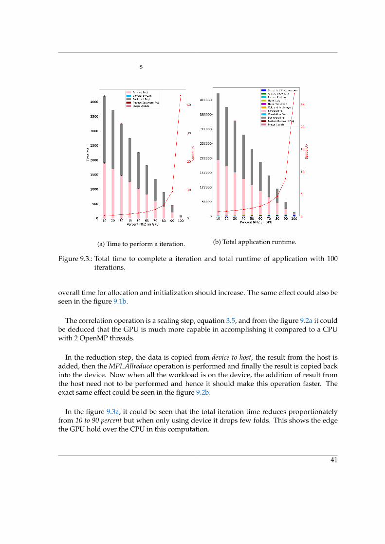
(a) Time to perform a iteration. (b) Total application runtime.

Figure 9.3.: Total time to complete a iteration and total runtime of application with 100iterations.

overall time for allocation and initialization should increase. The same effect could also beseen in the figure 9.1b9.1b.

The correlation operation is a scaling step, equation 3.53.5, and from the figure 9.2a9.2a it couldbe deduced that the GPU is much more capable in accomplishing it compared to a CPUwith 2 OpenMP threads.

In the reduction step, the data is copied from device to host, the result from the host isadded, then the MPI Allreduce operation is performed and finally the result is copied backinto the device. Now when all the workload is on the device, the addition of result fromthe host need not to be performed and hence it should make this operation faster. Theexact same effect could be seen in the figure 9.2b9.2b.

In the figure 9.3a9.3a, it could be seen that the total iteration time reduces proportionatelyfrom 10 to 90 percent but when only using device it drops few folds. This shows the edgethe GPU hold over the CPU in this computation.

41

9. Effect of Splitting Work between CPU and GPU

The figure 9.3b9.3b sheds light on how the use of even 1 GPU could reduce the computationtime by many folds. It is also interesting to note that when all the computation is happen-ing on the GPU, the allocation and initialization time is comparable to the time it takesto perform 100 iterations. This effect could also be seen in the profiling results shown inchapter 1313.

42

10. Performance vs Number of GPU

The purpose of this test is to determine the scaling of the implementation when the numberof MPI processes are increased from 1-8 with each connected to a GPU. This test was per-formed on DGX-1. The processes were bound to core and they were mapped by L3cache.The tests were performed 50 times for each increase in MPI processes with 10 iterations.So the results presented in figure 10.110.1 are calculated over 50 data points and the resultspresented in 10.210.2 are calculated over 500 data points.

(a) Time to Allocate and Initialize CSRand measured data

(b) Total time for Allocation and Initial-ization Operations.

Figure 10.1.: Time to perform Allocation and Initialization Operations.

The possible reason why the perfect scaling is not achieved in the allocation and copyingthe data on the devices,figure 10.1a10.1a, is because of the way the test was performed. Sincewe mapped the processes to the L3cache which means that we only use one of the CPU

43


and since each CPU has only two PCIe-3 x16 slots, which means that the total double datatransfer rate is 64 Gigabytes per second (GBps). Moreover, each PCIe-3 slot is directlyconnected to 2 GPUs and so each CPU has direct connection to only 4 GPUs and for therest of the GPUs the data transfer takes over NVlink. But we see the speedup as we increasethe number of MPI processes because not each MPI process asks the PCIe-3 slot to transferthe data at the same time and due to this staggering the data is loaded faster.

The figure 10.1b10.1b shows how the total time reduces as the number of MPI processes (witha GPU each) are increased from 1-8. The limitation on I/O, i.e RAM and storage, could beargued as the reason why the reading and conversion to CSR vectors of the system matrix(marked as blue) does not scale perfectly with the increase in number of MPI processes.

The figure 10.2a10.2a and figure 10.2b10.2b shows the effect on Forward Projection(SPMV) and Back-ward Projection (SPMV T) calculation time with increasing number of GPUs. These twooperation scales more than perfectly with the increasing number of GPUs and the reasonis the increase in total available atomic functional units. It could also be argued that this in-crease might be coming from the increasing total memory bandwidth but that is unlikely.It is so because the total amount of data that has to be read and written in each kernel is12838.6 + 5.3 + 3 = 12846.9 MegaBytes and the forward and backward projection kernels for1 GPU finishes in approximately 32.3 ms and 63.1 ms and in 4.0 ms and 7.3 ms for 8 GPUsrespectively. This gives a effective bandwidth of 397.7 GBps and 203.6 GBps in case of 1GPU which increases to 401.5 GBps and 220.0 GBps for 8 GPUs for forward and backwardprojection respectively while the theoretical maximum is 732 GBps.

The effect of increasing number of atomic functional units is more pronounced in the caseof backward projection because there are lot more total atomic operation in the backwardprojection, 1,327,104 vs 1,603,498,863 to be precise.

The figure 10.2c10.2c presents the typical behaviour of MPI Allreduce operation with the in-creasing number of MPI processes, i.e. increasing operation time with increasing MPIprocesses.

Finally, the figure 10.2d10.2d shows the decrease in total runtime for a iteration with increas-ing GPUs. Even though the forward and backward projection scaled more than perfectlywith increasing GPU, that effect is adversely affected by the MPI Allreduce time in theoverall iteration time.

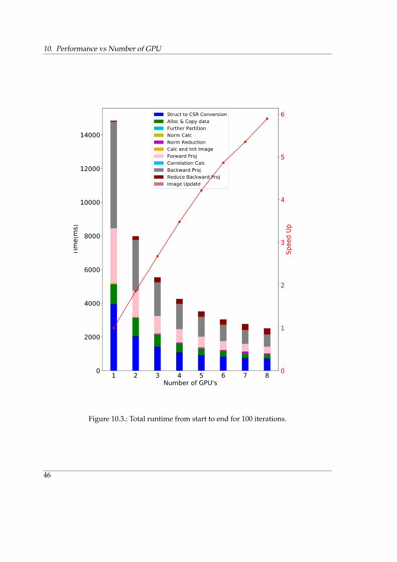
The figure 10.310.3 shows the total runtime of the implementation with 100 iterations andoverall it scales very well but not perfectly with increasing GPUs. This figure also tellsthat the GPUs could be used to reduce the problem runtime proportionately but for thatto happen, there should be lot more computation.

44

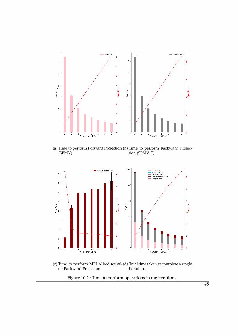
(a) Time to perform Forward Projection(SPMV)

(b) Time to perform Backward Projec-tion (SPMV T)

(c) Time to perform MPI Allreduce af-ter Backward Projection

(d) Total time taken to complete a singleiteration.

Figure 10.2.: Time to perform operations in the iterations.45


Figure 10.3.: Total runtime from start to end for 100 iterations.

46

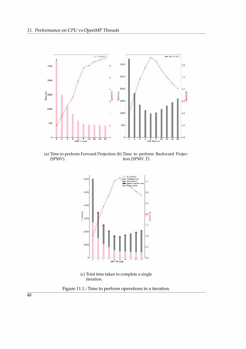
11. Performance on CPU vs OpenMP Threads

This test was performed to see the effect of how the implementation scales on the hostwhen more and more OpenMP threads are provided. For this test, a node was allocatedon the Mac Cluster and the application was launched with only 1 MPI process. The appli-cation was bound to the hwthread and the mapping was done per L3cache. The tests wereperformed 50 times with 10 iterations for each subsequent increase in OpenMP threadsavailable to the host.

The figure 11.1a11.1a and 11.1b11.1b show the effect of increasing openmp threads for the compu-tation of Forward Projection (SPMV) and Backward Projection (SPMV T) respectively. In boththe figures it could be seen that the increasing openmp threads have clear positive effect onthe time it takes to complete the computation upto 8 threads, although not proportionally.The reason for not seeing the proportional increase is because all the threads are mappedby the L3cache and hence are using the same host resources like Last Level Cache (LLC).

Now the reason for the very slow decrease in time taken to solve the Forward Projectionand even increase in time taken to solve the Backward Projection after 8 Openmp threads isdue to the fact that now the hyper-threading of the host kicks in. After 8 Openmp threads,the subsequent threads are allocated on the same core which has already one thread run-ning on it and due to this a lot of context switching takes place during the execution whichultimately degrades the performance. The effect is more pronounced in the case of Back-ward Projection because it uses a private array per thread to compute the SPMV T com-pared to none for computing SPMV in Forward Projection, which degrades the cache per-formance. The codes 11.111.1 and 11.211.2 are the host implementation of Forward and Backwardprojection respectively to show the use of private array per thread.

The figure 11.1c11.1c shows how the increase of openmp thread affects the performance ofa iteration in total. In the figure it could be seen that the performance increase only till 8openmp threads because after that the degradation in backward projection overwhelm theslight increase in performance for forward projection.

The table 11.111.1 shows the bandwidth achieved, per process and per thread, as the num-ber of OMP threads are increased from 1 to 16 when launching the application with 1 MPIprocess only. It shows that in the case of Forward projection the bandwidth increases aswe increase the OMP threads but falls with respect to per thread. In the case of Back-ward projection the bandwidth rises when the threads are increased from 1 top 8 but falls

47

11. Performance on CPU vs OpenMP Threads

(a) Time to perform Forward Projection(SPMV).

(b) Time to perform Backward Projec-tion (SPMV T).

(c) Total time taken to complete a singleiteration.

Figure 11.1.: Time to perform operations in a iteration.48

Operation(BW) \OMP Threads1 8 16

Process Thread Process Thread Process ThreadForward Projection (GBps) 4.59 4.59 26.7 3.34 30.47 1.90

Backward Projection (GBps) 3.88 3.88 12.25 1.53 7.87 0.49

Table 11.1.: CPU bandwidth per MPI process and per thread as a factor of increasing OMPthread when launching application with 1 MPI process.

when increase from 8 to 16. In this case also the bandwidth per thread keeps falling as weincrease the OMP threads.

1 #pragma omp parallel for schedule(dynamic)2 for (size_t row=further_split_for_cpu.start ;3 row< further_split_for_cpu.end ; ++row){4 float res = 0.0;5

6 std::for_each(matrix.beginRow2(row), matrix.endRow2(row),7 [&](const RowElement<float>& e){8 res += e.value()*image_mask[e.column()];});9 correlation[row] = res;

10 }

Source Code 11.1.: Forward projection on host.

1 #pragma omp parallel{2 Vector<float> pri_update(update.size(), 0.0);3 #pragma omp for schedule(dynamic)4 for (uint32_t row=further_split_for_cpu.start;5 row<further_split_for_cpu.end; ++row){6 std::for_each(matrix.beginRow2(row), matrix.endRow2(row),7 [&](const RowElement<float>& e){8 pri_update[e.column()]+=e.value()*correlation[row];});9 }

10 #pragma omp critical11 for (size_t i = 0; i < update.size(); ++i)12 update[i] += pri_update[i];13 }

Source Code 11.2.: Backward projection on host.

49

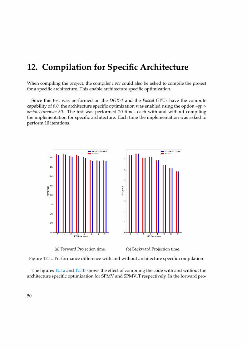
12. Compilation for Specific Architecture

When compiling the project, the compiler nvcc could also be asked to compile the projectfor a specific architecture. This enable architecture specific optimization.

Since this test was performed on the DGX-1 and the Pascal GPUs have the computecapability of 6.0, the architecture specific optimization was enabled using the option –gpu-architecture=sm 60. The test was performed 20 times each with and without compilingthe implementation for specific architecture. Each time the implementation was asked toperform 10 iterations.

(a) Forward Projection time. (b) Backward Projection time.

Figure 12.1.: Performance difference with and without architecture specific compilation.

The figures 12.1a12.1a and 12.1b12.1b shows the effect of compiling the code with and without thearchitecture specific optimization for SPMV and SPMV T respectively. In the forward pro-

50

jection the performance improves slightly when the code is compiled for the architecturebut in the case of backward projection the difference is almost non existent.

51

13. Profiling using NVVP

This test was performed to gauge the performance of different kernels using the NVIDIAVisual Profiler (NVVP). The test was performed with 1 MPI process. The test was performedon a virtual server with 16 virtual core and 1 Tesla P100 GPU. For profiling, the applicationwas run for 100 iterations.

The figure 13.113.1 shows the timeline generated for the implementation for 100 iterations.The interesting thing to note here that it takes only approximately 31.5 seconds from startto end and out of that almost 16 seconds are taken up by initialization steps. It can also beseen that since the memory was pinned, it takes around 1 second to free it.

The table 13.113.1 shows the occupancy for the kernels and the data transfer rate for thememory movement operations between host and device.

Kernel PerformanceCudaMemCpy (HtoD) Transfer Rate 11.3 - 11.6 GBpsCudaMemCpy (DtoH) Transfer Rate 10.4 - 10.7 GBps

SPMV T kernel time 64.5 msSPMV T kernel Occupancy 79.1 %

SPMV kernel time 31.6 msSPMV kernel Occupancy 98.9 %

Correlation Calculation kernel time 33 µsCorrelation Calculation kernel Occupancy 67.1%

Image update Kernel time 30 µsImage update Kernel Occupancy 82.3 %

Cublas Sum time 11.5 µsCublas Sum Occupancy 82.3 %

Cuda MemSet time 864 nsCuda MemSet Throughput 6144 GBps

Table 13.1.: Performance of kernels during the iterations.

52

Figu

re13

.1.:

App

licat

ion

profi

ling

usin

gN

VV

Pfo

r10

0it

erat

ions

.

53

Part III.

Future Work and Conclusion

54

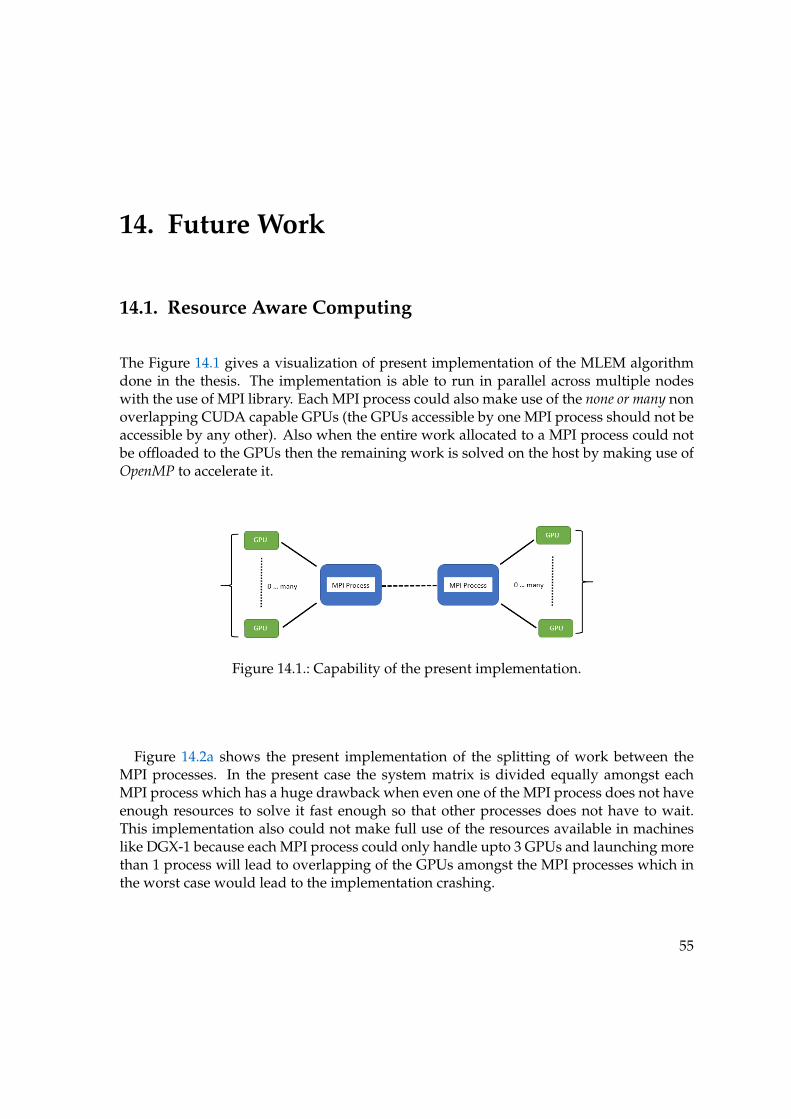
14. Future Work

14.1. Resource Aware Computing

The Figure 14.114.1 gives a visualization of present implementation of the MLEM algorithmdone in the thesis. The implementation is able to run in parallel across multiple nodeswith the use of MPI library. Each MPI process could also make use of the none or many nonoverlapping CUDA capable GPUs (the GPUs accessible by one MPI process should not beaccessible by any other). Also when the entire work allocated to a MPI process could notbe offloaded to the GPUs then the remaining work is solved on the host by making use ofOpenMP to accelerate it.

Figure 14.1.: Capability of the present implementation.

Figure 14.2a14.2a shows the present implementation of the splitting of work between theMPI processes. In the present case the system matrix is divided equally amongst eachMPI process which has a huge drawback when even one of the MPI process does not haveenough resources to solve it fast enough so that other processes does not have to wait.This implementation also could not make full use of the resources available in machineslike DGX-1 because each MPI process could only handle upto 3 GPUs and launching morethan 1 process will lead to overlapping of the GPUs amongst the MPI processes which inthe worst case would lead to the implementation crashing.

55

14. Future Work

(a) Not resource aware splitting of work

(b) Resource aware splitting of work

Figure 14.2.: Splitting of system matrix NNZs when the implementation is resource awareand when it is not.

All the above mentioned drawbacks could be ameliorated by using flowchart for split-ting the work shown in figure 14.2b14.2b. In the resource aware case, the MPI processes makesub communicators based on their host-names and the MPI processes in each sub com-municator splits the available resources amongst themselves. Now after deciding on theresources, each MPI process takes the chunk of the the system matrix that it can solve withthe results being ready at almost the same time as all other processes. This implementationleads to much better load balancing, faster execution and optimal resource utilization.

For example, when the resource aware implementation is used on the completely idleDGX-1 machine, it would split the system matrix in the ratio of 3/8 : 3/8 : 2/8 or 2/8 : 2/8 :

56

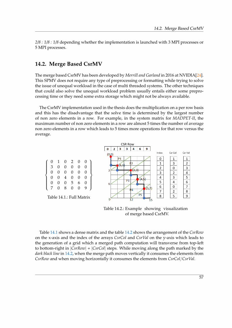
14.2. Merge Based CsrMV

2/8 : 1/8 : 1/8 depending whether the implementation is launched with 3 MPI processes or5 MPI processes.

14.2. Merge Based CsrMV

The merge based CsrMV has been developed by Merrill and Garland in 2016 at NVIDIA[2424].This SPMV does not require any type of preprocessing or formatting while trying to solvethe issue of unequal workload in the case of multi threaded systems. The other techniquesthat could also solve the unequal workload problem usually entails either some prepro-cessing time or they need some extra storage which might not be always available.

The CsrMV implementation used in the thesis does the multiplication on a per row basisand this has the disadvantage that the solve time is determined by the largest numberof non zero elements in a row. For example, in the system matrix for MADPET-II, themaximum number of non zero elements in a row are almost 5 times the number of averagenon zero elements in a row which leads to 5 times more operations for that row versus theaverage.

0 1 0 2 0 03 0 0 0 0 00 0 0 0 0 00 0 4 0 0 00 0 0 5 6 07 0 8 0 0 9

Table 14.1.: Full Matrix

Table 14.2.: Example showing visualizationof merge based CsrMV.

Table 14.114.1 shows a dense matrix and the table 14.214.2 shows the arrangement of the CsrRowon the x-axis and the index of the arrays CsrCol and CsrVal on the y-axis which leads tothe generation of a grid which a merged path computation will transverse from top-leftto bottom-right in |CsrRow| + |CsrCol| steps. While moving along the path marked by thedark black line in 14.214.2, when the merge path moves vertically it consumes the elements fromCsrRow and when moving horizontally it consumes the elements from CsrCol/CsrVal.

57

14. Future Work

For launching this algorithm on p threads, first the grid is divided into p parts diagonallyof equal width and then each thread determines it own path in the part allocated to it. Thestarting vertex for each thread (marked by red dots) could be determined by the constrainedbinary search along the first diagonal in the thread’s swath. More specifically, for anydiagonal k: the vertex (i,j) fulfills the condition that CsrRowi > all items before CsrColj and i+j = k. By using this approach the total work to be performed is of the order of O(|CsrRow|+ |CsrCol|).

58

15. Conclusion

In this work, the Maximum Likelihood Estimation Maximization (MLEM) algorithm for thePositron Emission Topography (PET) has been implemented making use of the GPUs whichhas been built upon the previous implementation of MLEM for multicore architectures.The implementation tries to offload the maximum amount of computation work on theGPUs. The remaining work is solved by the host to minimize the data transfer betweenthe host and device which ultimately leads to better performance. The work on the hostis further accelerated by the use of multiple threads using OpenMP. Moreover, the imple-mentation also gives user the option to specify some of the parameters for selecting theGPUs through the configuration file.

The first part of the thesis gives a short introduction to the PET scanners, their config-uration and why they are used. It also gives a mathematical foundation to the equationssolved in the MLEM algorithm, all of which has also been presented as a pseudo code.After that the Compressed Sparse Row (CSR) format to store the matrix has been explainedalong with the sample codes to show how the Sparse Matrix Vector Multiplication (SPMV)and Transpose Sparse Matrix Vector Multiplication (SPMV T) computations are performedusing this format. The architecture of the GPUs has been discussed briefly along withCUDA as a programming language, which has been used to write the kernels for NVIDIAGPUs in the thesis. Most of the discussion about CUDA has centered around the technolo-gies necessary to produce this work. It also discusses the optimization strategies from thehost as well as device side to gain extra performance.

The next part has focused mainly on the performance and scaling of the implementationunder different scenarios namely with respect to increasing number of OpenMP threadson the host, increasing number of GPUs and in the case when GPU memory alone is notenough. Apart from that, some of the tests also focuses on the performance improvementswith the use of Pinned Memory, CUDA Aware MPI, compilation of code for specific GPUarchitecture and using custom kernels. Many conclusions can be drawn from the thesetests, which can be summarized as follows:

• Although different MPI implementations are built upon the same standards, thereare still some noticeable performance differences between them.

• The pinned memory could be used to speed up all sort of data transfer i.e. betweenhost and device, between different MPI processes apart from I/O operations. But the

59

15. Conclusion

pinned memory should be used carefully as it takes more time to be allocated anddeallocated and could even degrade the performance in low memory systems.

• The implementation of the library functions should be understood before using them,especially CuSparse from NVIDIA, since they are not always the best as has been thecase with the SPMV T using CSR format shown in the thesis.

• For accelerating the performance of the host code, the OpenMP threads should notbe increased blindly as they not always lead to better performance.

• Compiling the code for a specific architecture not always leads to better performancein every kernels but since it does not degrades the performance, the codes should becompiled architecture specific whenever possible.

During the course of working on the implementation and later during the tests, therehave been times when unexpected behaviour has been observed. An educated guess couldbe made to explain some of these behaviours but not for all of them. Further tests areneeded to explain these behaviours. They are as follows:

• On the K20 machine in the LRR chair, if the code is launched with only ./implementa-tion it does not detect the GPU which is not the case when launched like mpirun -n 1./implementation.

• The reason for OpenMPI being slower in the first allreduce operation in the imple-mentation compared to Intel MPI while being faster after that on the Mac Cluster isstill not well understood.

• The reason for the slight difference in results between CPU and GPU is probably dueto different floating point arithmetic implementations but it still require further teststo be sure.

• The unexpected performance hit when using Cuda Aware MPI warrants furtherscrutiny.

• A single MPI process could only handle upto 3 GPUs which is possibly due to I/Olimitations but more research is need to be completely sure.

In hindsight, it could be said that the implementation is performing as intended underdifferent scenarios. The implementation is able to adapt to the hardware it is being runon and perform satisfactorily. The two major performance bottlenecks could be solved bychanging the splitting of system matrix from equally among MPI processes now to be moreresource aware and by changing the implementation of SPMV T to merge based SPMV Twhich promises better performance and higher GPU occupancy.

60

Appendix

61

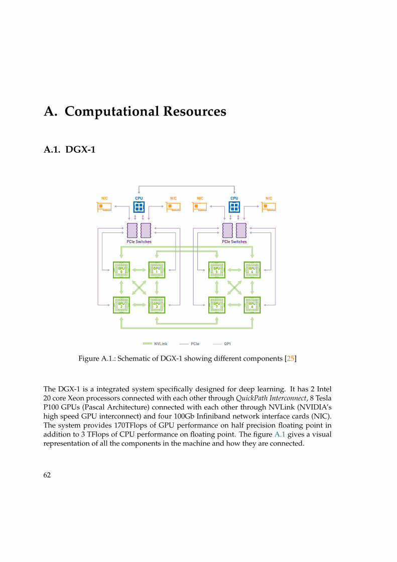
A. Computational Resources

A.1. DGX-1

Figure A.1.: Schematic of DGX-1 showing different components [2525]

The DGX-1 is a integrated system specifically designed for deep learning. It has 2 Intel20 core Xeon processors connected with each other through QuickPath Interconnect, 8 TeslaP100 GPUs (Pascal Architecture) connected with each other through NVLink (NVIDIA’shigh speed GPU interconnect) and four 100Gb Infiniband network interface cards (NIC).The system provides 170TFlops of GPU performance on half precision floating point inaddition to 3 TFlops of CPU performance on floating point. The figure A.1A.1 gives a visualrepresentation of all the components in the machine and how they are connected.

62

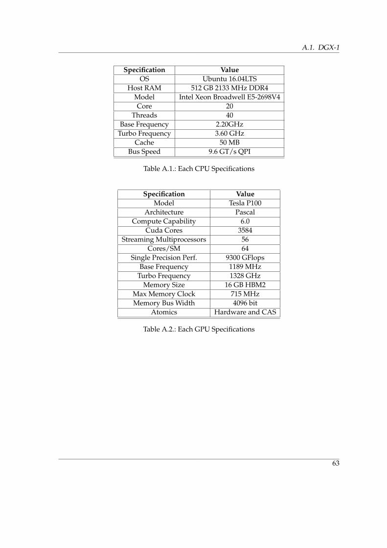
A.1. DGX-1

Specification ValueOS Ubuntu 16.04LTS

Host RAM 512 GB 2133 MHz DDR4Model Intel Xeon Broadwell E5-2698V4Core 20

Threads 40Base Frequency 2.20GHz

Turbo Frequency 3.60 GHzCache 50 MB

Bus Speed 9.6 GT/s QPI

Table A.1.: Each CPU Specifications

Specification ValueModel Tesla P100

Architecture PascalCompute Capability 6.0

Cuda Cores 3584Streaming Multiprocessors 56

Cores/SM 64Single Precision Perf. 9300 GFlops

Base Frequency 1189 MHzTurbo Frequency 1328 GHz

Memory Size 16 GB HBM2Max Memory Clock 715 MHzMemory Bus Width 4096 bit

Atomics Hardware and CAS

Table A.2.: Each GPU Specifications

63

A. Computational Resources

A.2. Mac Cluster

Mac cluster is made up of 4 nodes where each node is dual socket Intel SandyBridge-EPXeon E5-2670 with 2 NVIDIA M2090 GPUs and FDR Infiniband. The table A.3A.3 and A.4A.4 listthe specification of CPU and GPU in more detail.

Specification ValueHost RAM/node 128 GB

Model Intel SandyBridge-EP Xeon E5-2670Core 8

Threads 16Base Frequency 2.60GHz

Turbo Frequency 3.30 GHzCache 20 MB

Bus Speed 8.0 GT/s QPI

Table A.3.: Each CPU Specifications

Specification ValueModel Tesla M2090

Architecture FermiCompute Capability 2.0

Cuda Cores 512Streaming Multiprocessors 16

Cores/SM 32Single Precision Perf. 1331 GFlops

Base Frequency 1300 MHzMemory Size 6 GB GDDR5

Max Memory Clock 1850 MHzMemory Bus Width 384 bit

Atomics lock/update/unlock

Table A.4.: Each GPU Specifications

64

B. Compiling and Using CUDA AwareOpenMPI on Mac Cluster

To compile the CUDA Aware OpenMPI on Mac Cluster follow these steps.

• First of all allocate one of the node from nvd partition and then ssh into it. The rea-son for this is that the files required for NUMA support are available on the computenodes and not on the login node. Also don’t forget to unload any other MPI imple-mentation.

• Download the OpenMPI 1.10.7 by executing wget http://www.open-mpi.de/software/ompi/v1.10/downloads/openmpi-1.10.7.tar.gz

• Extract the file by tar -xvzf openmpi-1.10.7.tar.gz

• Go into the folder by cd openmpi-1.10.7

• Configure the OpenMPI by executing ./configure –prefix=$HOME/.openmpi –with-cuda=/lrz/sys/parallel/cuda/7.5/cuda/include CFLAGS=-D LP64 –with-wrapper-cflags=”-DLP64 -ta:tesla”

The compiler flags CFLAGS=-D LP64 –with-wrapper-cflags=”-D LP64 -ta:tesla”are required with NVIDIA driver version 7.5 for things to work correctly.

• Next execute make

• Next execute make install

• Next close the ssh connection and go bask to the login node

• Put these 2 commands in bashrc

export PATH=$PATH:$HOME/.openmpi/bin

export LD LIBRARY PATH=$LD LIBRARY PATH:$HOME/.openmpi/lib

To compile the code with the newly installed OpenMPI, unload any other MPI imple-mentation and add

LFlags += -L$(HOME)/.openmpi/libIFlags += -I$(HOME)/.openmpi/include

Now launch the code normally.

65

C. Compiling NVML library on Mac Cluster

The NVML library has been used to check the available and total memory of the GPUsapart from checking the device temperature, core utilization and memory utilization. Thislibrary is installed with the CUDA Toolkit by default from version 8 onwards but thatis not the case with the toolkit available in the Mac Cluster (Version 7.5). So to install itmanually perform the following operations

• wget http://developer.download.nvidia.com/compute/cuda/7.5/Prod/gdk/gdklinux amd64 352 79 release.run

• chmod +x gdk linux amd64 * release.run

• ./gdk linux amd64 * release.run

• Link the library with the project in the Makefile.

66

D. Notes on MLEM Implementation

• Programming Language: C++

• Compilers

– mpicxx : For compiling .cpp and .c files. Intel MPI library version 5.1.3 for MacCluster and OpenMPI version 1.10.7 for DGX-1.

– nvcc : For compiling .cu files. CUDA version 7.5.17 on Mac Cluster and CUDAVersion 9.1.85 on DGX-1.

• Compilation Flags

– -O3 : For level 3 optimization

– -std=c++11 : For using C++ 11 standard.

• Flags used with nvcc

– -lcublas : For performing blas operations on NVIDIA GPUs.

– -lcusparse : For performing sparse operations on NVIDIA GPUs.

– -lmpi : To be able to compile code with MPI.

– -lnvidia-ml : To be able to use NVML library.

– -lboost system -lboost filesystem : To be able to use components of the BOOSTlibrary

– -Xcompiler -fopenmp : To compile files using OpenMP.

– -lgomp : To be able to link the files using OpenMP.

– –gpu-architecture=Value : To compile the code for specific architecture. TheValue is sm 20 for Mac Cluster and sm 60 for DGX-1.

• Configuration File : The parameters in the configuration files are as follows

– max devices to use : Allows the user to set the maximum number of GPUs eachprocess could use. Allowed range is [0,3]. Default value is 3.

– max nnz per device : Allows the user to define how many non zeros be of-floaded on each GPU. Allowed range is [0 , non zeros per rank]. Default valueis non zeros per rank.

– max temp allowed : Maximum GPU temperature to be selected. Allowed rangeis [0,100]. Default value is 100.

67

D. Notes on MLEM Implementation

– min free mem req : Minimum memory percentage of GPU to be free for itsselection. Allowed range is [0,100]. Default value is 100.

– max mem uti allowed : Maximum memory percentage utilization of GPU forits selection. Allowed range is [0,100]. Default value is 100.

– max gpu uti allowed : Max compute power percentage utilization of GPU forits selection. Allowed range is [0,100]. Default value is 100.

NOTE: Any of the parameter in the configuration file could be set to default by provid-ing values out of range (negative included). If implementation does not find any configu-ration file it will use the Default values.

68

Bibliography

[1] D. L. Bailey, D. W. Townsend, P. E. Valk, and M. N. Maisey, Positron emission tomogra-phy. Springer, 2005.

[2] A. Berger, “How does it work?: Positron emission tomography,” BMJ: British MedicalJournal, vol. 326, no. 7404, p. 1449, 2003.

[3] T. Kustner, J. Weidendorfer, J. Schirmer, T. Klug, C. Trinitis, and S. Ziegler, “Parallelmlem on multicore architectures,” in International Conference on Computational Science.Springer, 2009, pp. 491–500.

[4] M. Defrise, P. E. Kinahan, and C. J. Michel, “Image reconstruction algorithms in pet,”in Positron Emission Tomography. Springer, 2005, pp. 63–91.

[5] L. A. Shepp and Y. Vardi, “Maximum likelihood reconstruction for emission tomog-raphy,” IEEE transactions on medical imaging, vol. 1, no. 2, pp. 113–122, 1982.

[6] H. M. Hudson and R. S. Larkin, “Accelerated image reconstruction using orderedsubsets of projection data,” IEEE transactions on medical imaging, vol. 13, no. 4, pp.601–609, 1994.

[7] C.-M. Chen and S.-Y. Lee, “On parallelizing the em algorithm for pet image recon-struction,” IEEE Transactions on Parallel and Distributed Systems, vol. 5, no. 8, pp. 860–873, 1994.

[8] D. S. Lalush and B. M. Tsui, “Performance of ordered-subset reconstruction algo-rithms under conditions of extreme attenuation and truncation in myocardial spect,”The Journal of Nuclear Medicine, vol. 41, no. 4, p. 737, 2000.

[9] J. Dongarra, “Compressed row storage (crs),” 1995. [Online]. Available:http://netlib.org/linalg/html templates/node91.htmlhttp://netlib.org/linalg/html templates/node91.html

[10] C. Nvidia, “Cuda c programming guide, version 9.1,” NVIDIA Corp, 2018.

[11] J. Nickolls and D. Kirk, “Graphics and computing gpus,” Computer Organization andDesign: The Hardware/Software Interface, DA Patterson and JL Hennessy, 4th ed., MorganKaufmann, pp. A2–A77, 2009.

[12] N. Wilt, The cuda handbook: A comprehensive guide to gpu programming. Pearson Edu-cation, 2013.

70

http://netlib.org/linalg/html_templates/node91.html

Bibliography

[13] N. T. Nvidia, “P100 gpu,” Pascal Architecture White Paper, 2016.

[14] N. Gupta, “Texture memory in cuda,”http://cuda-programming.blogspot.de/2013/02/texture-memory-in-cuda-what-ishttp://cuda-programming.blogspot.de/2013/02/texture-memory-in-cuda-what-is-texture.html-texture.html.

[15] M. Harris, “How to access global memory effi-ciently in cuda c/c++ kernels,” 2013. [Online]. Available:https://devblogs.nvidia.com/how-access-global-memory-efficiently-cuda-c-kernelshttps://devblogs.nvidia.com/how-access-global-memory-efficiently-cuda-c-kernels

[16] N. Bell and M. Garland, “Efficient sparse matrix-vector multiplication on cuda,”Nvidia Technical Report NVR-2008-004, Nvidia Corporation, Tech. Rep., 2008.

[17] M. Boyer, “Pinned vs. non-pinned memory.” [Online]. Available:https://www.cs.virginia.edu/∼mwb7w/cuda support/pinned tradeoff.htmlhttps://www.cs.virginia.edu/∼mwb7w/cuda support/pinned tradeoff.html

[18] N. Gupta, “Bank conflicts in shared memory in cuda,”http://cuda-programming.blogspot.de/2013/02/bank-conflicts-in-shared-memoryhttp://cuda-programming.blogspot.de/2013/02/bank-conflicts-in-shared-memory-in-cuda.html-in-cuda.html.

[19] C. Nvidia, “Pascal tuning guide, version 9.1,” NVIDIA Corp, 2018.

[20] J. Kraus. (2013) An introduction to cuda-aware mpi. [Online]. Available:https://devblogs.nvidia.com/introduction-cuda-aware-mpi/https://devblogs.nvidia.com/introduction-cuda-aware-mpi/

[21] D. Fleisch and J. Kregenow, A Student’s Guide to the Mathematics of Astronomy. Cam-bridge University Press, 2013, chapter 1.

[22] D. Goldberg, “What every computer scientist should know about floating-point arith-metic,” ACM Computing Surveys (CSUR), vol. 23, no. 1, pp. 5–48, 1991.

[23] W. Kahan, “Ieee standard 754 for binary floating-point arithmetic,” Lecture Notes onthe Status of IEEE, vol. 754, no. 94720-1776, p. 11, 1996.

[24] D. Merrill and M. Garland, “Merge-based parallel sparse matrix-vector multiplica-tion,” in Proceedings of the International Conference for High Performance Computing, Net-working, Storage and Analysis. IEEE Press, 2016, p. 58.

[25] M. Harris, “Nvidia dgx-1: The fastest deep learning system,” 2017. [Online].Available: https://devblogs.nvidia.com/dgx-1-fastest-deep-learning-system/https://devblogs.nvidia.com/dgx-1-fastest-deep-learning-system/

71

http://cuda-programming.blogspot.de/2013/02/texture-memory-in-cuda-what-is

-texture.html

https://devblogs.nvidia.com/how-access-global-memory-efficiently-cuda-c-kernels

https://www.cs.virginia.edu/~mwb7w/cuda_support/pinned_tradeoff.html

http://cuda-programming.blogspot.de/2013/02/bank-conflicts-in-shared-memory

-in-cuda.html

https://devblogs.nvidia.com/introduction-cuda-aware-mpi/

https://devblogs.nvidia.com/dgx-1-fastest-deep-learning-system/

computational science and engineering (international master’s … · 2019-05-23 · 8. effect of...

Documents