Computational Sustainability: Smart Buildings

Manish MarwahSenior Research Scientist

Hewlett Packard Labsmanish.marwah@hpe.com

CS 325: Topics in Computational Sustainability, Spring 2016

Building Energy Use

http://energy.gov/sites/prod/files/ReportOnTheFirstQTR.pdf

3

Building Energy ManagementBuildings consume a lot of energy• Commercial buildings

• 1.3 trillion kWh electricity annually 1/3 of total US electricity generation

• Annual energy costs > $100 billion

Poorly maintained, degraded, and improperly controlled equipment wastes 15-30%energy in commercial buildings

Outline

• Meter placement• Anomaly detection• Occupancy Modeling• Energy Disaggregation

5

Where should meters be installed?

How can we detect anomalouspower consumption behavior?

How can we detect degradedperformance of equipment/devices in a buildings?

AbnormalNormal Abnormal

Ref.: KDD 2012, ACM BuildSys 2011, 2012

How can we cheaply measure building occupancy?

6

Test Bed

• HP Labs, Palo Alto, CA campus • Three buildings instrumented with ~40 power meters

Electrical Infrastructure Topology

7

Campus Power Use

• Power consumption characteristics of Buildings 1, 2 and 3

• Building 3 has a 135kW PV array

0

1

2

3

Main B1 B2 B3

AveragePeak

MW

Building Power Instrumentation

Where do I place the meters?

9

Building Power Instrumentation

Motivation: Obtain per-panel power consumption

Challenge: Large number of panels, each power meter: $1K-$3K

Goal: Select optimal locations for meter deployment

Approach: Formulate as an optimization problem over panel hierarchy (a tree structure)

10

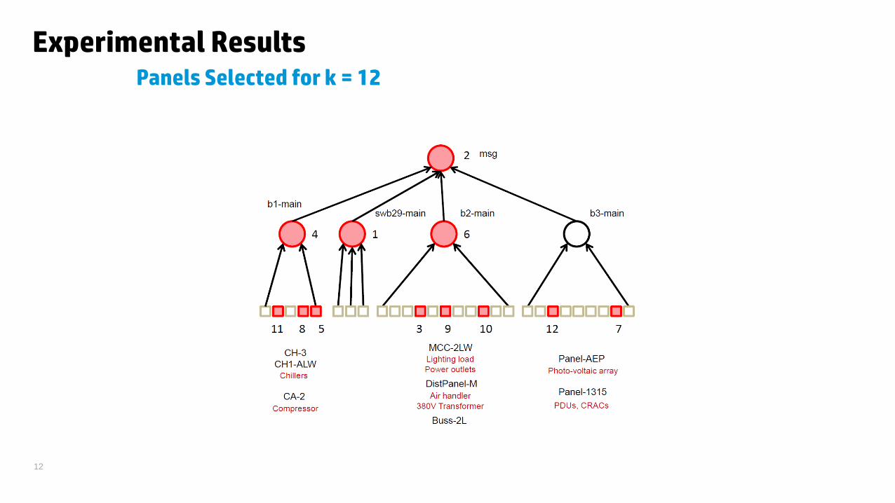
Panel Topology & Problem Formulation

Panel feeding load(s)

Panel feeding multiple sub-panels

: Set of all possible locations

: Set of all leaf locations

&

Panel TopologyProblem Formulation

: Selected locations

Select k meters:

: Set of meters

11

Greedy, Near-optimal Solution• Optimal solution is NP-hard

• Greedy optimization: Select panels sequentially

• We show objective function is submodular [KDD 2012]

• Thus, solution is guaranteed to be near-optimal [Krause et al. 2006]

~63%

12

Experimental ResultsPanels Selected for k = 12

13

Experiment Results

Number of meters installed (k)

RM

S P

redi

ctio

n er

ror a

t un

met

ered

pan

els

( x 1

00%

)

Prediction ability of the panels selected using the proposed approach

Building Power Management

Meter Anomaly Detection

15

Anomaly Detection

Motivation: • Abnormal power usage may indicate:

- wasted power- Failed or faulty equipment

Challenge: Obtaining labeled data is expensive• requires a lot of manual effort

Goal: Systematically detect abnormal power usage

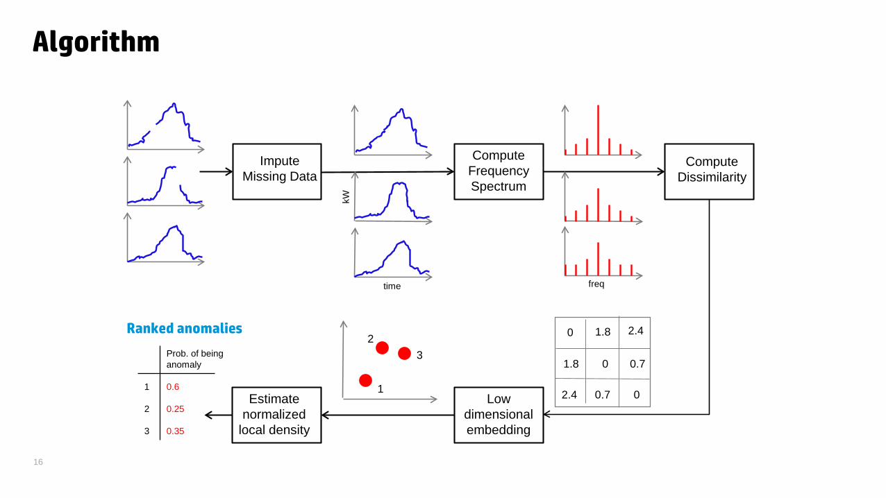
Approach: Use an unsupervised approach

16

Algorithm

Impute Missing Data

Compute Frequency Spectrum

Compute Dissimilarity

Low dimensional embedding

0

0

0

1.8 2.4

0.71.8

2.4 0.71

23

Estimate normalized

local density

1

2

3

0.6

0.25

0.35

Prob. of being anomaly

time freq

kW

Ranked anomalies

17

Anomaly ExamplesPower Saving Opportunities

Load: Air Handling Units in Building 2Anomaly:

• Abnormal time usage; Potential savings ~450 kWh

Load: Overhead Lighting in Building 1Anomalies:

• Abnormal low usage (holiday)• Abnormal time usage; Potential savings ~180

kWh

Building Power Management

Occupancy Modelling

19

Building Occupancy EstimationFor optimal resource provisioning

• Motivation: Save energy via occupancy-based lighting/air conditioning (HVAC) scheduling

• Challenge: Fine-grained occupancy information is not available, and requires additional sensors

– Expensive– Intrusive

• Goal: Accurately estimate occupancy of a zone using readily available data

• Approach– Use L2 port-level network statistics as a proxy– Semi-supervised method with minimal training data

Methodology[2]

[2] Bellala et.al., “Towards an understanding of campus-scale power consumption,” ACM BuildSys 2011.

k-st

ate

HM

MC

lass

ifier

Other features: Time of day, Day of week,

etc

Two stage Semi-supervised Approach – Can efficiently incorporate external parameters– Requires less training data

20

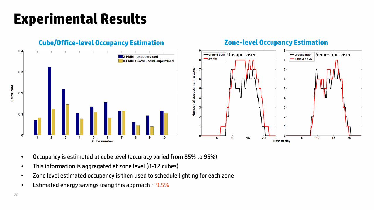
Experimental Results

Cube/Office-level Occupancy Estimation Zone-level Occupancy Estimation

• Occupancy is estimated at cube level (accuracy varied from 85% to 95%)

• This information is aggregated at zone level (8-12 cubes)

• Zone level estimated occupancy is then used to schedule lighting for each zone

• Estimated energy savings using this approach ~ 9.5%

Unsupervised Semi-supervised

Building Power Management

Energy Disaggregation

→

22

Residential Energy Consumption

“… the typical American household … is also likely to use 20 percent to 30 percent more energythan necessary…”

ACEEE, a non-profit advocacy group

“… Americans could cut their electricity consumption by 12 percent and save at least $35 billion over the next 20 years”

ACEEE, a non-profit advocacy group

23

http://www.withoutagym.net/wp-content/uploads/2014/02/LOWEST-GROCERY-BILL-EVER1.jpg

24

http://thumbs.dreamstime.com/z/electricity-bill-1565154.jpg

25

http://www.edisonfoundation.net/

GO BEYOND SMART METERS– Give customers breakdown of consumption

Energy Disaggregation

http://blog.lr.org/wp-content/uploads/2013/08/LordKelvin.jpg

ENERGY DISAGGREGATION

SOLUTION

–Install a meter on every appliance• Too intrusive• Too expensive

–Non-intrusive load monitoring (NILM) [George Hart, 1984]• Figure out appliance usage from the whole house measurement

PROBLEM STATEMENT

– Input• Y = <y1, y2, …, yT>, a sequence of aggregated power consumption• M, the number of appliances

– Output• S1= <s1, s2, …, sT>, a sequence of consumption for Appliance 1• S2= <s1, s2, …, sT>, a sequence of consumption for Appliance 2

…• SM= <s1, s2, …, sT>, a sequence of consumption for Appliance M

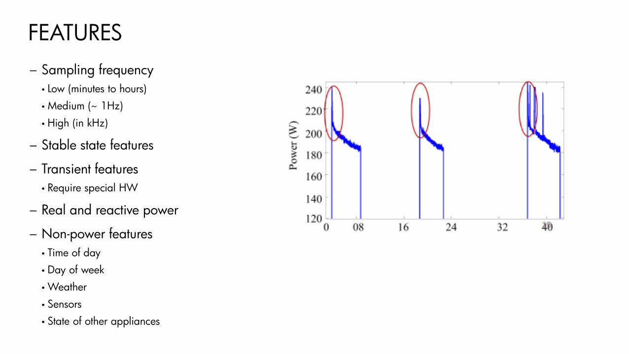
FEATURES– Sampling frequency

• Low (minutes to hours)• Medium (~ 1Hz)• High (in kHz)

– Stable state features

– Transient features• Require special HW

– Real and reactive power

– Non-power features• Time of day• Day of week• Weather• Sensors• State of other appliances

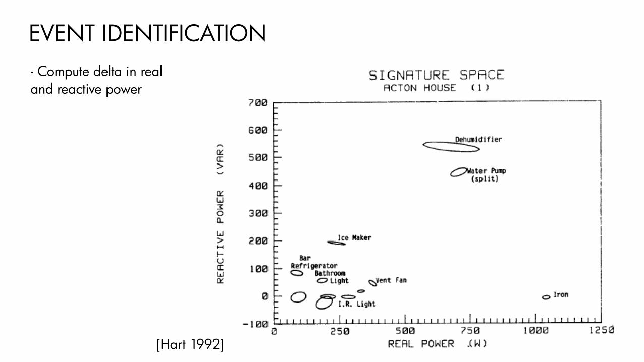
EVENT IDENTIFICATION- Compute delta in real and reactive power

[Hart 1992]

APPLIANCE STATE MACHINES

[Hart 1992]

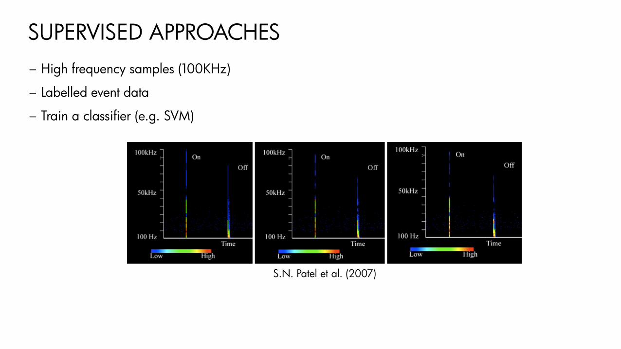
SUPERVISED APPROACHES– High frequency samples (100KHz)

– Labelled event data

– Train a classifier (e.g. SVM)

S.N. Patel et al. (2007)

DRAWBACKS OF EVENT-BASED METHODS

–Require labelled data

–Events considered in isolation

–Most require high frequency data

HMM-BASED MODELS– General algorithm outline

– 1. Define a model

– 2. Learn the parameters in the model from data

– 3. Make predictions (Inference)

HMM

Time 1 2 3 4 5 6 7 8 …readings 2.5 2.4 1.0 1.1 1.7 1.6 0.8 0.7 …

A 1.4 1.5 0 0 0 0 0 0 …B 1.1 0.9 1.0 1.1 1.0 0.9 0 0 …C 0 0 0 0 0.7 0.8 0.8 0.7 …

2.5 2.4 1.0

ON, ON, OFF ON, ON, OFF OFF, ON, OFFtransition

state

emission

HIDDEN MARKOV MODEL– Transition probability

Pr(st+1 = i | st = j ) = πij

– Emission probabilityPr(yt = v | st = i) ~ Normal(wi, e), where e is the noise variance

2.5 2.4 1.0

ON, ON, OFF ON, ON, OFF OFF, ON, OFFtransition

state

emission

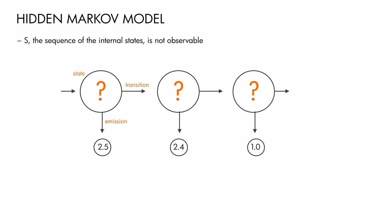
HIDDEN MARKOV MODEL– S, the sequence of the internal states, is not observable

2.5 2.4 1.0

ON, ON, OFF ON, ON, OFF OFF, ON, OFFtransition

state

emission

? ? ?

HIDDEN MARKOV MODEL– Transition probability

Pr(st+1 = i | st = j ) = πij

– Emission probabilityPr(yt = v | st = i) ~ Normal(wi, e), where e is the noise variance

– Let θ = {πij} U {wi} U {e}, the set of the parameters in HMM

– If both S and Y are observable, we can find the parameters θ by Maximum Likelihood (ML)

– But… S is unknown

– If Y and θ are known, we can perform inference to compute S

– Chicken and egg problem!

– Expectation Maximization (EM)

HIDDEN MARKOV MODEL– The number of states: 2M

– The number of parameters: 2M + 22M

• 2M emission-parameters• 22M transition-parameters

– Exponential increase with number of appliances

– That’s too many parameters!

FACTORIAL HIDDEN MARKOV MODEL– The number of states: 2M

– The number of parameters: 6M• 2M emission-parameters• 4M transition-parameters

– Much better!

FACTORIAL HIDDEN MARKOV MODEL– Assumption: Appliances are used independently

– The observation is a linear combination of the emissions of the markov chains

2.5 2.4 1.0

OFF OFF OFF

ON ON ON

ON ON OFF

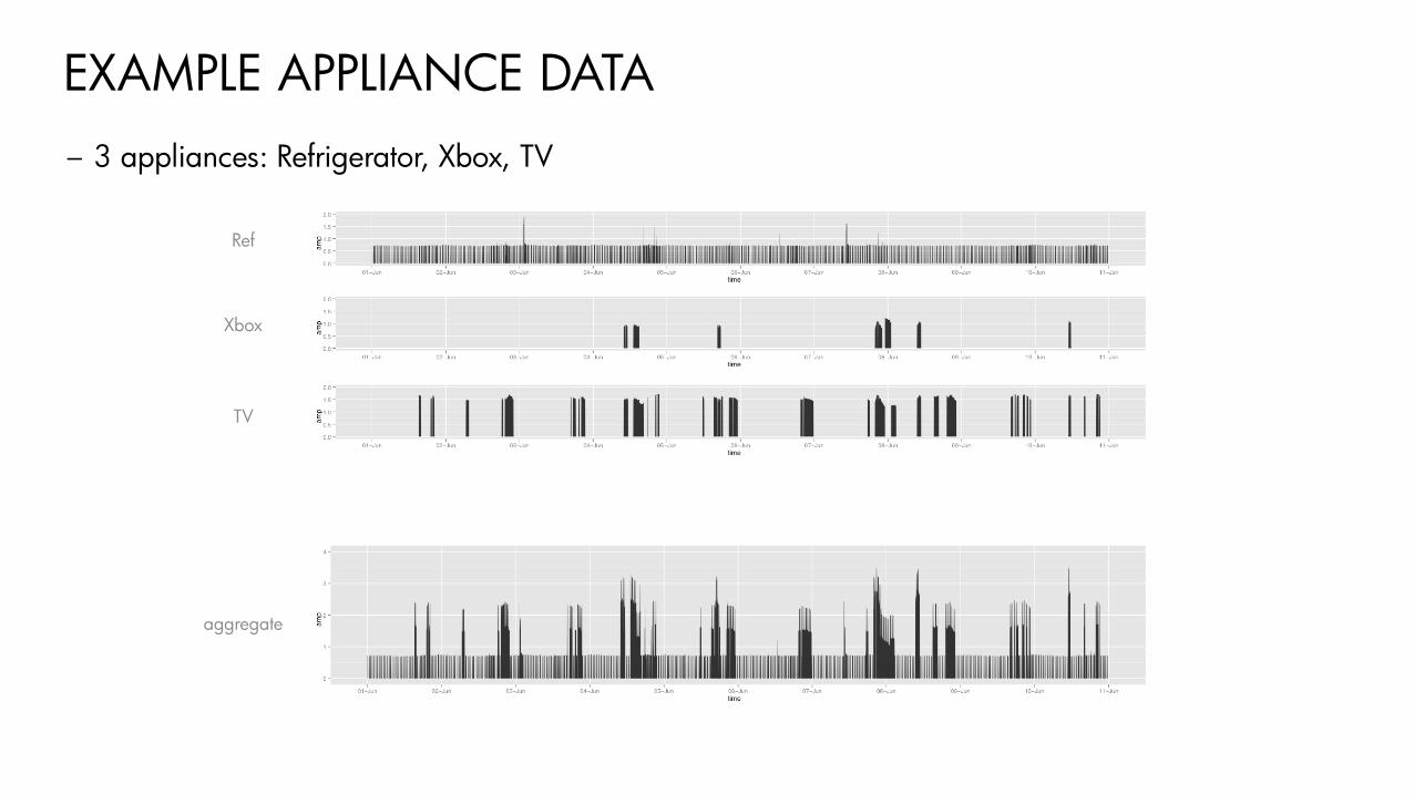
EXAMPLE APPLIANCE DATA– 3 appliances: Refrigerator, Xbox, TV

Ref

Xbox

TV

aggregate

APPLIANCE DISTRIBUTIONSpower consumption refrigerator

television xbox

FHMM – EM ITERATION 0power consumption refrigerator

television xbox

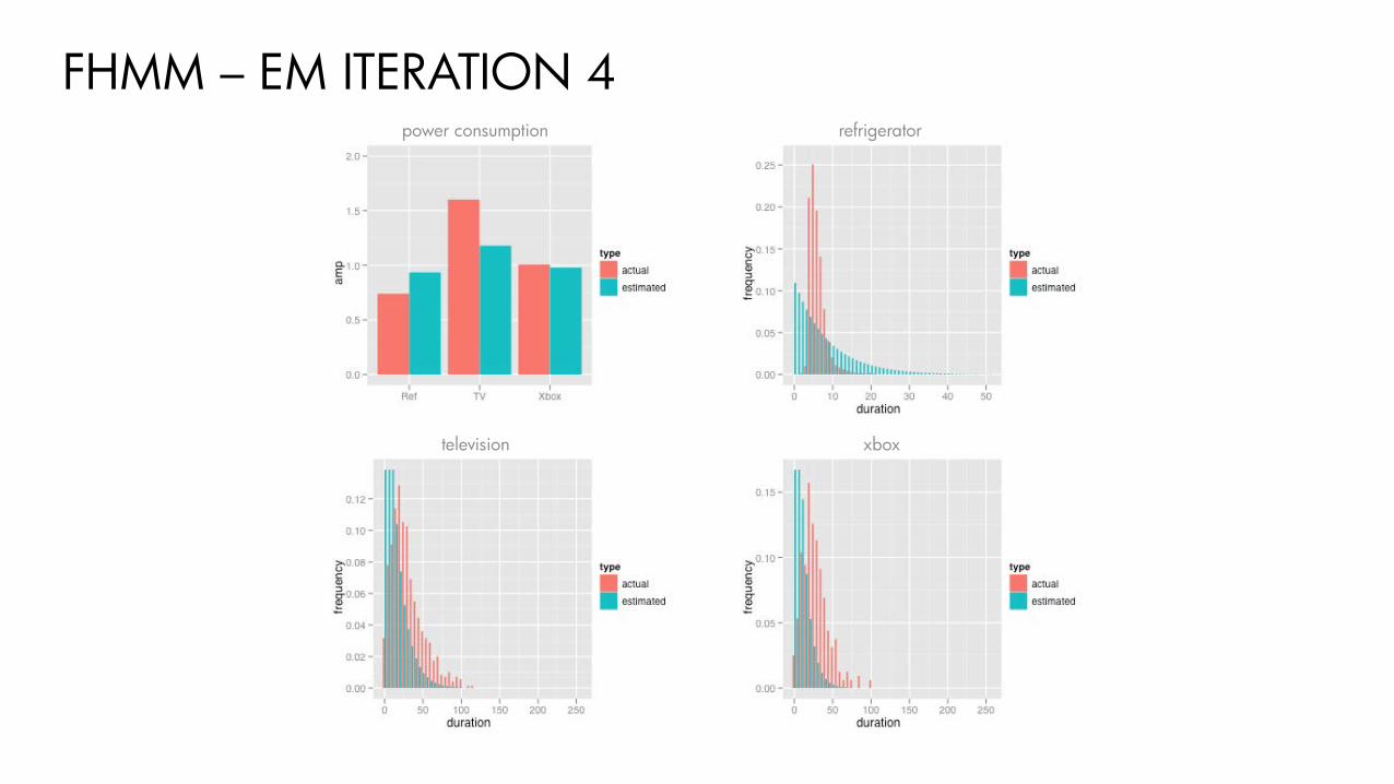
FHMM – EM ITERATION 4power consumption refrigerator

television xbox

FHMM – EM ITERATION 10power consumption refrigerator

television xbox

FHMM – EM ITERATION 20power consumption refrigerator

television xbox

CHALLENGE:STATE-DURATION DISTRIBUTIONS– In the family of Hidden Markov Model, the state-durations have exponential distributions

– But, the state-durations for appliances follow gamma distributions

Exponential distribution Gamma distribution

images from http://en.wikipedia.org/

FACTORIAL HIDDEN SEMI-MARKOV MODEL

0.7

ON

OFF

OFF

3.2

ON

ON

ON

3.1

ON

ON

ON

1.1

OFF

ON

OFF

1.6

OFF

OFF

ON

Pr(d1=2) Pr(d1=5)

Pr(d2=3)

Pr(d3=3)

FHSMM – EM ITERATION 0power consumption refrigerator

television xbox

FHSMM – EM ITERATION 1power consumption refrigerator

television xbox

FHSMM – EM ITERATION 5power consumption refrigerator

television xbox

FHSMM – EM ITERATION 10power consumption refrigerator

television xbox

FHSMM – EM ITERATION 20power consumption refrigerator

television xbox

FHMM vs. FHSMM

power consumption refrigerator televisionxbox

CHALLENGE:MODELING DEPENDENCIES– There are many factors which affect the usage of appliances

– There can be additional contextual features

– Example• Weather (e.g. heater, A/C)• Day of the week (e.g. more TV on the weekends)• Time of day (e.g. more Xbox in the afternoon)• Seasons (e.g. more laundry in summer)• User’s schedule (e.g. more laptop use in early morning)• Other appliances (e.g. TV is on when Xbox is in use)

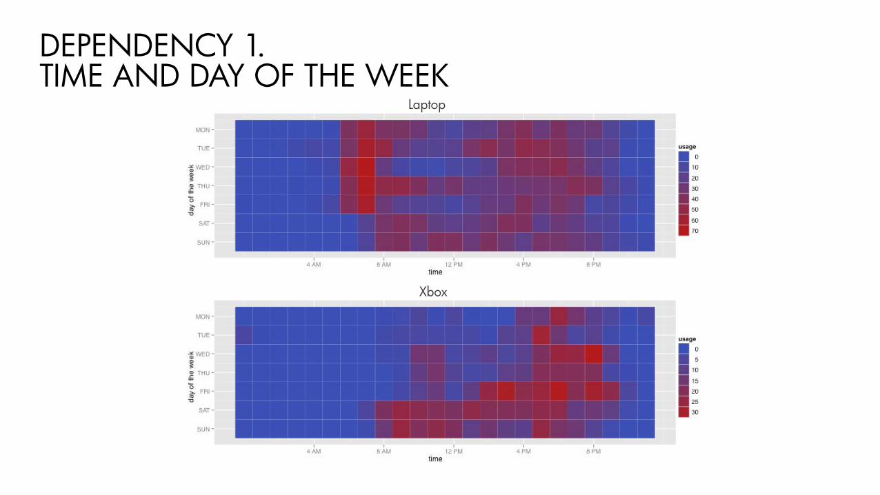
DEPENDENCY 1.TIME AND DAY OF THE WEEK

Laptop

Xbox

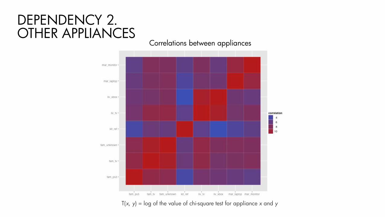
DEPENDENCY 2.OTHER APPLIANCES

T(x, y) = log of the value of chi-square test for appliance x and y

Correlations between appliances

CONDITIONAL FACTORIAL HIDDEN MARKOV MODEL

– In FHMM, the transition probability is constant

– In CFHMM, the transition probability depends on several conditions, and it is computed by assuming each condition is independent (Naïve Bayes assumption)

where Z is the normalization factor

APPLIANCE STATISTICSpower consumptions

appliance correlations

refrigerator

xbox

television

CFHMM – RESULT

refrigerator

xbox

television

refrigerator

xbox

television

Actual Estimated

CONDITIONAL FACTORIAL HIDDEN SEMI-MARKOV MODEL

FHMM FHSMM

CFHMM CFHSMM

RESULTS

Acknowledgements

Martin Arlitt, Cullen Bash, Gowtham Bellala, Hyungsul Kim, Geoff Lyon, Martha Lyons, Chandrakant Patel

References

• [SIAM 2011] Hyungsul Kim, Manish Marwah, Martin Arlitt, Geoff Lyon and Jiawei Han, "Unsupervised Disaggregation of Low Frequency Power Measurements", SIAM International Conference on Data Mining (SDM 11), Mesa, Arizona, April 28-30, 2011.• [BuildSys 2011] Gowtham Bellala, Manish Marwah, Martin Arlitt, Geoff Lyon, Cullen Bash, "Towards an understanding of campus-scale power consumption." In ACM BuildSys, November 1, 2011, Seattle, WA.• [BuildSys 2012] G. Bellala, M. Marwah, A. Shah, M. Arlitt, C. Bash, "A Finite State Machine-based Characterization of Building Entities for Monitoring and Control", Proceedings of ACM Workshop on Building Systems (Buildsys), Nov 2012.• [KDD 2012] Gowtham Bellala, Manish Marwah, Martin Arlitt, Geoff Lyon, Cullen Bash, "Following the Electrons: Methods for Power Management in Commercial Buildings." In KDD, August 12-16, 2012, Beijing, China.• [Hart 1992] Hart, G.W., ``Nonintrusive Appliance Load Monitoring," Proceedings of the IEEE, December 1992, pp. 1870-1891.