1

COMPUTATIONAL TECHNIQUES

LABORATORY

LAB MANUAL

Year : 2018-2019

Subject Code : BCCB25

Regulations : IARE-R18

Semester : I

Branch : CAD/CAM

Prepared By

Dr. K. Viswanath Allamraju

Professor

Department of Mechanical Engineering

INSTITUTE OF AERONAUTICAL ENGINEERING (Autonomous)

Dundigal, Hyderabad-500043

2

INSTITUTE OF AERONAUTICAL ENGINEERING (Autonomous)

Dundigal, Hyderabad - 500 043

MECHANICAL ENGINEERING

Program Outcomes

PO1 Apply advanced level knowledge, techniques, skills and modern tools in the field of

computer aided engineering to critically assess the emerging technological issues.

PO2 Have abilities and capabilities in developing and applying computer software and

hardware to mechanical design and manufacturing fields.

PO3 Conduct experimental and/or analytical study and analyzing results with modern

mathematical / scientific methods and use of software tools.

PO4 Function on multidisciplinary environments by working cooperatively, creatively and

responsibly as a member of a team.

PO5 Write and present a substantial technical report / document.

PO6 Independently carry out research / investigation and development work to solve

practical problems.

PO7 Design and validate technological solutions to defined problems and recognize the

need to engage in lifelong learning through continuing education.

3

COMPUTATIONAL TECHNIQUE LABARATORY SYLLABUS

Week-1 INTRODUCTION TO MATLAB PROGRAM

Applications to MATLAB in Mechanical Engineering.

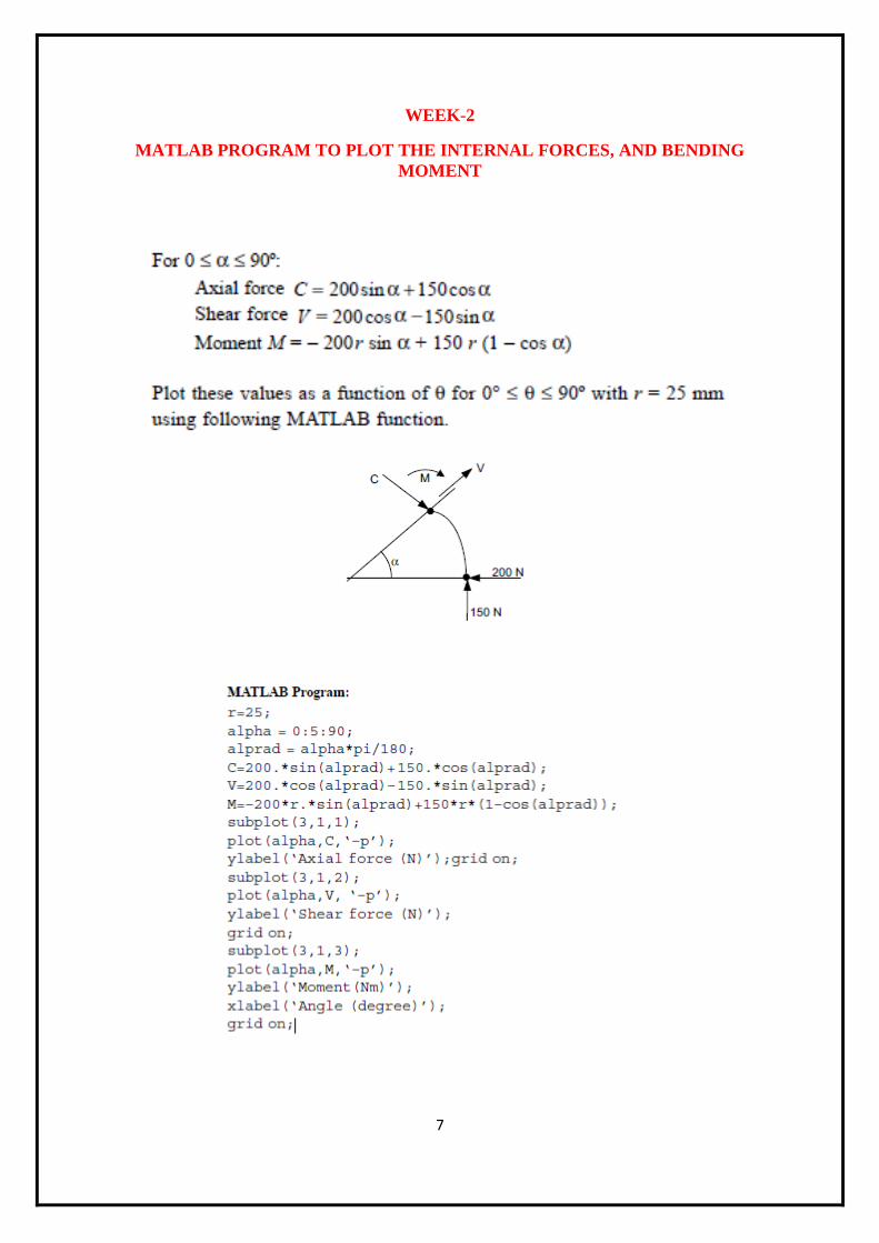
Week-2 MATLAB PROGRAM TO PLOT THE INTERNAL FORCES, AND BENDING

MOMENT.

The radius of the semicircular member is 25 mm and supported with roller and hinged supports. The load 300N

acting vertically downward at the center and 200 N acting horizontally at the roller support toward left direction

Write a MATLAB program to plot the internal forces, namely, the axial forces, shearing force and bending

moment as functions of α for 0 < α < 90º.

Week-3 THERMAL STRESS ANALYSIS OF PISTON USING MATLAB PROGRAM

Temperature distribution around the given piston dimensions.

Week-4 FORMULATION OF IDEAL AND REAL GAS EQUATIONS.

Gas phase thermodynamic equations of state relate the three state variables of temperature, pressure, and volume for a gas. One of the three state variables can be calculated through the equation of state if values for the other two variables are known. For example, the ideal gas law states PV = RT ~ where P : pressure, Pa: V : specific or molar gas volume, m

3 mol R : ideal gas constant, (= 8.314 J/(mol K)) T : absolute

temperature, K

Week-5 USING MATLAB PROGRAM PLOT THE FUNCTION OF ONE VARIABLE AND TWO

VARIABLES

Graphing-functions of one variable and two variables

Week-6 MULTI BODY DYNAMIC ANALYSIS THROUGH MATLAB PROGRAM

Use of MATLAB to solve simple problems in vibration, Mechanism Simulation using multi body dynamic

software

Week-7 MATLAB PROGRAM FOR EULERS EQUATION OF MOTION

Solution of Difference Equations using Euler Method.

Week-8 MATLAB PROGRAM FOR CURVE FITTING.

Determination of polynomial using method of Least Square Curve Fitting.

4

Week-9 DYNAMIC ANALYSIS USING MATLAB PROGRAM

Dynamics and vibration analysis

Plot the response of the system using MATLAB for n=5rad/s, = 0.05, 0.1, 0.2 subjected to the initial

conditions x(0) = 0, (0) xo = v0 = 60 cm/s.

Week-10 MATLAB PROGRAM TO PLOT THE RESULTANT ACCELERATION AND THE

VARIATION OF ACCELERATION PROGRAM

A jet plane is going in a parabolic path described by y=0.05x2. At a point in the path, it has a velocity of 200

m/s, which is increasing at the rate of 0.8 m/s2. Find the resultant acceleration and plot the variation of

acceleration as a function of its horizontal position x.

ATTAINMENT OF PROGRAM OUTCOMES

& PROGRAM SPECIFIC OUTCOMES

Exp.

No.

Experiment

Program Outcomes

Attained

1 Introduction to MATLAB. PO1, PO3, PO5

2 Solving of PDE PO1, PO2, PO5

3 Using MATLAB program plot the function of one variable and two variable

PO1, PO2, PO3, PO5

4 MATLAB program to plot the internal forces, and bending moment.

PO1, PO3, PO5

5 Thermal stress analysis of piston using MATLAB program PO2, PO3,PO5

6 Multi body dynamic analysis through MATLAB program PO1, PO2, PO3

7 Analysis of kinematics in 4 bar mechanism PO2, PO3, PO5

8 MATLAB program for curve fitting PO2, PO3,PO5

9 Dynamic analysis using MATLAB program PO1, PO2, PO3

10 Variation of acceleration with total acceleration PO2, PO3, PO5

5

WEEK-1

APPLICATIONS OF MAT-LAB IN MECHANICAL ENGINEERS

Introduction

MATLAB is a high-level language and interactive environment for numericalcomputation,

visualization, and programming. Using MATLAB, you can analyse data, develop algorithms, and

create models and applications. The language, tools, and built-inmath functions enable you to

explore multiple approaches and reach a solution fasterthan with spread sheets or traditional

programming languages, such as C/C++ or Java. You can use MATLAB for a range of applications,

including signal processing andcommunications, image and video processing, control systems, test

and measurement, computational finance, and computational biology. More than a million

engineers andscientists in industry and academia use MATLAB, the language of technical

computing.

Strengths

MATLAB may behave as a calculator or as a programming language

MATLAB combine nicely calculation and graphic plotting.

MATLAB is relatively easy to learn

MATLAB is interpreted (not compiled), errors are easy to fix

MATLAB is optimized to be relatively fast when performing matrix

operations

MATLAB does have some object-oriented elements

Weaknesses

MATLABis not a general purpose programming language such as C, C++, or

FORTRAN.

MATLAB is designed for scientific computing, and is not well suitable for other

applications

MATLAB is commercial software and a trademark of The MathWorks, Inc., USA. It is an

integrated programming system, including graphical interfaces and a large number of

specialized toolboxes. MATLAB is getting increasingly popular in all fields of science and

engineering.

Some capabilities of MATLAB in Mechanical Engineering are:

1. Structural Analysis

2. Computational Fluid Dynamics

3. Thermal Analysis

4. Analysis of composite structures

5. Industrial Production technology

6

6. Control systems

MATLAB is extensively used in Defence, Space technology, Aerospace and Automobile

industries because of its application in modelling and finite element analysis. It is also used in

Mass production industries.

MATLAB's Power of Computational Mathematics

MATLAB is used in every facet of computational mathematics. Following are some commonly used mathematical calculations where it is used most commonly:

Dealing with Matrices and Arrays

2-D and 3-D Plotting and graphics

Linear Algebra

Algebraic Equation

Non-linear Functions

Statistic

Data Analysis

Calculus and Differential Equations

Numerical Calculations

Integration

Transforms

Curve Fitting

Various other special functions

7

WEEK-2

MATLAB PROGRAM TO PLOT THE INTERNAL FORCES, AND BENDING

MOMENT

8

9

WEEK-3

THERMAL STRESS ANALYSIS OF PISTON.

SOFTWARE REQUIRED

1. MATLAB R2013a.

2. Windows 7/XP SP2.

PROCEDURE

1. Open MATLAB

2. Open new M-file

3. Type the program

4. Save in current directory

5. Compile and Run the program

6. For the output see command window\ Figure window

PROGRAM

PISTON FUNCTION AND ASSOCIATED PROBLEM AREAS

The function of the piston is to absorb the energy by the gas / air which enters in the

cylinder and then accelerates to produce useful mechanical energy. So to prevent the

leakage & proper compressor of air /gas the piston must be sealed with the cylinder surface.

This is accomplished by the piston rings which also help to prevent oil from entering in the

cylinder from underneath the piston. Another function of the rings is to keep the piston from

contacting the cylinder wall. Less contact area between the cylinder and piston reduces

friction, thereby increasing efficiency. As a result of this process, heat is transferred from

the combustion gases into the piston and other components that makeup the cylinder walls.

This reduces the thermodynamic efficiency of the process, and therefore also diminishes

power.

PISTON COOLING

The reduction of Temperature in the piston can be done by heat pipe cooling method. This

system allows for a channel inside the piston skirt that directs heat away from the piston

itself. This will increases the heat transfer through the piston, which does not help the

efficiency of the compressor, but we can use the special light alloys to form the piston.

Magnesium and its alloys have much larger creep rates than other metals and therefore can

usually not sustain the same load and temperatures as steel or aluminium. A heat pipe

system can drastically reduce the temperature of the piston crown from about 700ºC to only

350ºC.Therefore, using heat-pipe technology makes it easier to employ magnesium alloys in

10

pistons. Cooling gallery pistons are manufactured with water soluble salt cores or as

‘‘cooled ring carriers’’ with a sheet metal cooling gallery attached to the ring carrier. An

adjusted jet with a fixed housing injects the cooling oil into the annular cooling gallery

through an inlet orifice in the piston. Maintaining the correct quantity of oil decisively

influences heat dissipation. The outlet is formed by one or more bores inside a piston,

preferably positioned on the side of the cooling gallery approximately opposite the inlet.

PISTON TEMPERATURE DISTRIBUTION

Generally the heat flux is highest in the centre of the cylinder head, in the exhaust valve seat

region, and to the centre of the piston. Cast-iron pistons run about40 to 800 C h otter than

aluminium pistons. In the flat topped piston the centre of the crown is hottest and the outer

edge cooler by 20 to 500 C. The maximum temperatures occur where the heat flux is high

and access for cooling is difficult. Such locations are the bridge between the valves and the

region between the exhaust valves of adjacent cylinders. The heat generated by friction

between the piston and the liner is a significant fraction of the liner thermal loading.

Temperature distributions in the piston can be calculated from the knowledge of the heat

fluxes across the component surface using finite element analysis techniques. For steady-

state engine operation, the depth within a component to which the unsteady temperature

fluctuations (caused by the variations in heat flux during the cycle) penetrate is small, so a

quasi-steady solution is satisfactory. In this finite element analysis, the actual piston shape

was approximated with a three-dimensional grid for one quadrant of the piston. A standard

finite element analysis

of the heat flow through the piston yields the temperature distribution within the piston. The

thermal stresses can therefore be calculated and added to the mechanical stress field to

determine the total stress distribution. This can be used to define the potential fatigue

regions in the actual piston design.

DESIGN DATA OF COMPRESSOR:

• Power Capacity : 5 H.P

• Speed : 1440 R.P.M

• Piston Displacement : 500 LPM

• Atmospheric Pressure : 1.01325 bar

• Working Pressure : 10 bar • Temperature on top surface of Piston: 158.530 C

The above data is taken for the design of piston through which various geometries of the

piston can be found out which are mentioned below. The material of the piston is Aluminium alloy 6061. Design of the Piston can be done by general programme in

MATLAB Software.

PROGRAMME IN MATLAB

clc

11

clear

k=0.04

n=1.25

p1=input('Enter the Value of atm. Pressure')

p3=input('Enter the Value of working Pressure')

p2=sqrt(p1*p3)

% VE=Volumetric

Efficiency VE=1-

(k*((p2/p1)^(1/n)-1))

% ME=Mechanical Efficiency

% BP=Brake Power

% IP=Indicated Power

% WD=Work

Done ME=0.80

BP=input('Enter the Value of Brake

Power') IP=(ME)*(BP)

WD=(IP)*60

R=0.287

T1=273

T2=T1*((p2/p1)^((n-

1)/n))

% T1=atm. Temperature

% T2=Intermediate Temperature

% m=Mass of Air Delivery

m=(WD*(n-1))/(R*n*((p2/p1)^((n-1)/n)-1)*(T1+T2))

m1=m/60

FAD=Free Air Delivery

% N=Revolution per Minute

N=1440

FAD=(m1*R*T2*10)/(p2*10

*)

% Vs=Swept

Volume

Vs=FAD/VE

% L=Stroke of Piston

% D=Diameter of Piston

% th=Thickness of head

% ts=Tensile Stress

% p=Working

Pressure p=1

ts=56.4

th=sqrt((3*p*(D1^2))/(16*ts))

ts=input('Enter the Value of Tensile Stress')

% t1=Radial Thickness of

Piston Ring Pw=0.035

t1=D1*(sqrt((3*Pw)/ts))

% mu=Coefficient Of Friction

% R=Maximum Side Thrust

mu=0.1

12

R=(mu*pi*(D1^2)*p)/4

% l=Length of Piston skirt

% Pb=Bearing

Pressure Pb=0.25

l=R/(Pb*D1) The above programme is for Design of Piston of Reciprocating air Compressor. By entering various Input parameter we can get the Output of the Programme which shows the design of Piston.

OUTPUT

k = 0.0400

n = 1.2500

Enter the Value of atm. Pressure1.01325

p1 = 1.0133 bar

Enter the Value of working Pressure14

p3 = 14 bar

p2 = 3.7664 bar

VE = 0.9257

ME = 0.8000

Enter the Value of Brake Power 3.73 KW

BP =3.7300 KW

IP =2.9840 KW

WD =179.0400 KW

R = 0.2870 KJ/Kg K

T1 =273 K

T2 = 354.9799 K

m = 0.6616 kg/sec

m1 = 0.0110 kg/min

N =1440 R.P.M

FAD = 2.0714 x 10 -6 m3

Vs = 2.2377 x 10 -6 m3

L = 0.1000 m

D = 0.0534 m

D1 = 53.3777 mm

p = 1 N/mm2

ts = 56.4000 mm

th =3.0777 mm

Enter the Value of Tensile Stress19.6 N/mm2

ts =19.6000 mm

Pw = 0.0350 N/mm2

t1 = 3.9068 mm

mu = 0.1000

R = 223.7736 N

Pb = 0.2500 N/mm2

l = 16.7691 mm

13

WEEK-4

FORMULATION OF IDEAL AND REAL GAS EQUATIONS

SOFTWARE REQUIRED

1. MATLAB R2013a.

2. Windows 7/XP SP2.

PROCEDURE

1. Open MATLAB

2. Open new M-file

3. Type the program

4. Save in current directory

5. Compile and Run the program

6. For the output see command window\ Figure window

PROGRAM

The gas law, for example,

P = f(n,T,V) [ = nRT/V]

if you give the function values for n,T,V, the function returns a value for P. The formula in

brackets is what the ideal gas law would use to compute the value of the function, but other

formula could also be used.

In Matlab, we would write such a function for the ideal gas law like this:

function P = idealP(V)

% computes pressure using the ideal gas law

% for 1 mole

% assumes the temperature is 293

R = .08206;

T = 293.0;

n = 1.0;

P = n*R*T./V;

Important things to note:

The first word in the file is function.

The variable to be computed, P, is on the left

The name of the function appears to the right of =and is followed by parameters or arguments to be supplied when the function is called.

Somewhere in the function body, the variable P must be given value.

14

All variables used in the function are local> to the function.

If you expect to send in a vector as an argument, make certain any formulas in the function

can handle vectors.

A more general version, as a function of n,V,T:

Function P = ideal P(n,V,T)

% computes pressure using the ideal gas law for given values of n,V,T

% can compute P for a range of V

R = .08206;

P = n*R*T. /V;

15

WEEK-5

USING MATLAB PROGRAM PLOT THE FUNCTION OF ONE VARIABLE AND

TWO

VARIABLES

Line plot

Bar graph

Surface plot

Contour plot

MATLAB tutorial on 2D, 3D visualization tools as well as other graphics packages available

in our tutorial series.

Line Plot

>> t = 0:pi/100:2*pi;

>> y = sin(t);

>> plot(t,y)

Line Plot – continues

>> xlabel('t');

>> ylabel('sin(t)');

>> title('The plot of t vs sin(t)');

16

Line Plot – continues

>> y2 = sin(t-0.25);

>> y3 = sin(t+0.25);

>> plot(t,y,t,y2,t,y3) % make 2D line plot of 3 curves

>> legend('sin(t)','sin(t-0.25)','sin(t+0.25',1)

Customizing Graphical Effects

Generally, MATLAB’s default graphical settings are adequate which makes plotting fairly

effortless. For more customized effects, use the get and set commands to change the

behaviour of specific rendering properties.

17

>>> hp1 = plot(1:5) % returns the handle of this line plot

>> get(hp1) % to view line plot's properties and their values

>> set(hp1, 'lineWidth') % show possible values for line Width

>> set(hp1, 'lineWidth', 2) % change line width of plot to 2

>> gcf % returns current figure handle

>> gca % returns current axes handle

>> get(gcf) % gets current figure's property settings

>> set(gcf, 'Name', 'My First Plot') % Figure 1 => Figure 1: My First Plot

>> get(gca) % gets the current axes. property settings

>> figure(1) % create/switch to Figure 1 or pop Figure 1 to the front

>> clf % clears current figure

>> close % close current figure; "close 3" closes Figure 3

>> close all % close all figures

2D Bar Graph

>> x = magic(3); % generate data for bar graph

>> bar(x) % create bar chart

>> grid % add grid for clarity

18

Save a Plot with print

To add a legend, either use the legend command or use the insert command in the Menu Bar

on the figure. Many other actions are available in Tools.

It is convenient to use the Menu Bar to change a figure’s properties interactively. However,

the set command is handy for non-interactive changes, as in an m-file.

Similarly, save a graph via the Menu Bar’s File/’Save as’ or

>> print -djpeg 'mybar' % file mybar.jpg saved in current dir

Use MATLAB Command Syntax or Function Syntax?

Many MATLAB utilities are available in both command and function forms.

For this example, both forms produce the same effect:

>> print -djpeg 'mybar' % print as a command

>> print('-djpeg', 'mybar') % print as a function

For this example, the command form yields an unintentional outcome:

>> myfile = 'mybar'; % myfile is defined as a string

>> print -djpeg myfile % as a command, myfile is 'myfile' (verbatim), not 'mybar'

>> print('-djpeg', myfile) % as a function, myfile is treated as a variable

Other frequently used utilities that are available in both forms are save and load

Surface Plot

>> Z = peaks; % generate data for plot

>> surf(Z) % surface plot of Z

19

Try these commands to see their effects:

>> shading flat

>> shading interp

>> shading faceted

>> grid off

>> axis off

>> colorbar

>> colormap('winter')

>> colormap('jet')

Contour Plots

>> Z = peaks;

>> contour(Z, 20) % contour plot of Z with 20 contours

20

>> contourf(Z, 20); % with color fill

>> colormap('hot') % map option

>> colorbar % make color bar

Integration Example

21

WEEK-6

MULTI BODY DYNAMIC ANALYSIS THROUGH MATLAB PROGRAM

Simscape™ Multibody™ models are similar in composition to the systems they represent. A

typical model comprises bodies, joints and constraints, forces and torques, and sensors. Start

your model by creating the subsystems that represent the bodies. Then, connect the

subsystems with joints and constraints to define kinematic relationships. To measure the

dynamic response of system components, add forces and torques—or, equivalently, motion

inputs—to drive the model and sensors.

Bodies Model body geometries, inertias, colors, and frames

Assembly Connect bodies through joints, gears, and constraints

Dynamics Apply and sense force, torque, and motion

Applications Examples of real-world multibody systems

Bodies

Model body geometries, inertias, colors, and frames

Model the bodies of an articulated mechanical assembly. Bodies can be rigid or flexible, the

latter being free to deform when acted upon by a force or torque. All bodies are characterized

by their physical properties, among them geometry, inertia, and color. Flexible bodies have

the additional properties of stiffness, damping, and discretization level.

Rigid bodies are based on the various solid blocks, the File Solid block, or, in special cases,

their equivalents of variable mass and geometry. You can find the latter in the Body

Elements > Variable Mass library. Use the File Solid block to import a body from a 3-D

part file. Flexible bodies are based on the General Flexible Body block—a representation of a

slender body with a specified cross section.

A single Brick Solid, File Solid, or General Flexible Beam block may suffice to completely

model a body. More often, several are required. The body is then a composite of simpler

body elements fixed to one another. Frame connection lines between the blocks establish the

necessary rigid connections between the body elements. Rigid Transform blocks, normally

inserted in the connection lines, provide the relative positions and orientations required for

proper assembly.

22

Dynamics

Apply and sense force, torque, and motion

Add forces, torques, and motion inputs to drive your model and use sensors to measure its

dynamic response. Use the joint blocks in your model to actuate those joints, model their

internal mechanics, and sense joint-specific dynamic variables. Only Joints blocks allow you

to specify trajectories in a model.

Use Forces and Torques blocks to model interactions between unconnected bodies or to add

special dynamic elements such as gravitational fields and nonlinear spring-dampers—the

latter using the generic Internal Force block. You can sense the relative motions of

unconnected bodies using the Transform Sensor block.

Specify Joint Actuation Torque

Model Overview

In Simscape™ Multibody™, you actuate a joint directly using the joint block. Depending on

the application, the joint actuation inputs can include force/torque or motion variables. In this

example, you prescribe the actuation torque for a revolute joint in a four-bar linkage model.

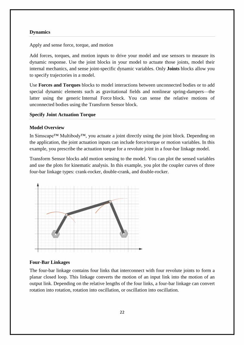
Transform Sensor blocks add motion sensing to the model. You can plot the sensed variables

and use the plots for kinematic analysis. In this example, you plot the coupler curves of three

four-bar linkage types: crank-rocker, double-crank, and double-rocker.

Four-Bar Linkages

The four-bar linkage contains four links that interconnect with four revolute joints to form a

planar closed loop. This linkage converts the motion of an input link into the motion of an

output link. Depending on the relative lengths of the four links, a four-bar linkage can convert

rotation into rotation, rotation into oscillation, or oscillation into oscillation.

23

Links

Links go by different names according to their functions in the four-bar linkage. For example,

coupler links transmit motion between crank and rocker links. The table summarizes the

different link types that you may find in a four-bar linkage.

Link Motion

Crank Revolves with respect to the ground link

Rocker Oscillates with respect to the ground link

Coupler Transmits motion between crank and rocker links

Ground Rigidly connects the four-bar linkage to the world or another subsystem

It is common for links to have complex shapes. This is especially true of the ground link,

which may be simply the fixture holding the two pivot mounts that connect to the crank or

rocker links. You can identify links with complex shapes as the rigid span between two

adjacent revolute joints. In example Model a Closed-Loop Kinematic Chain, the rigid span

between the two pivot mounts represents the ground link.

Linkages

The type of motion conversion that a four-bar linkage provides depends on the types of links

that it contains. For example, a four-bar linkage that contains two crank links converts

rotation at the input link into rotation at the output link. This type of linkage is known as a

double-crank linkage. Other link combinations provide different types of motion conversion.

The table describes the different types of four-bar linkages that you can model.

Linkage Input-Output Motion

Crank-rocker Continuous rotation-oscillation (and vice-versa)

Double-Crank Continuous rotation-continuous rotation

Double-rocker Oscillation-oscillation

Grashof Condition

The Grashof theorem provides the basic condition that the four-bar linkage must satisfy so

that at least one link completes a full revolution. According to this theorem, a four-bar

24

linkage contains one or more crank links if the combined length of the shortest and longest

links does not exceed the combined length of the two remaining links. Mathematically, the

Grashof condition is:

s+l ≤ p+q

where:

s is the shortest link

l is the longest link

p and q are the two remaining links

Grashof Linkages

A Grashof linkage can be of three different types:

Crank-rocker

Double-crank

Double-rocker

By changing the ground link, you can change the Grashof linkage type. For example, by

assigning the crank link of a crank-rocker linkage as the ground link, you obtain a double-

crank linkage. The figure shows the four linkages that you obtain by changing the ground

link.

Modeling Approach

In this example, you perform two tasks. First you add a torque actuation input to the model.

Then, you sense the motion of the crank and rocker links with respect to the World frame.

The actuation input is a torque that you apply to the joint connecting the base to the crank

25

link. Because you apply the torque at the joint, you can add this torque directly through the

joint block. The block that you add the actuation input to is called Base-Crank Revolute Joint.

You add the actuation input to the joint block through a physical signal input port. This port

is hidden by default. To display it, you must select Provided by Input from

the Actuation > Torque drop-down list.

You can then specify the torque value using either Simscape or Simulink® blocks. If you use

Simulink blocks, you must use the Simulink-PS Converter block. This block converts the

Simulink signal into a physical signal that Simscape Multibody can use. For more

information, see Actuating and Sensing with Physical Signals.

To sense crank and rocker link motion, you use the Transform Sensor block. With this block,

you can sense motion between any two frames in a model. In this example, you use it to sense

the [Y Z] coordinates of the crank and rocker links with respect to the World frame.

The physical signal output ports of the Transform Sensor blocks are hidden by default. To

display them, you must select the appropriate motion outputs. Using the PS-Simulink

Converter, you can convert the physical signal outputs into Simulink signals. You can then

connect the resulting Simulink signals to other Simulink blocks.

In this example, you output the crank and rocker link coordinates to the workspace using

Simulink To Workspace blocks. The output from these blocks provide the basis for phase

plots showing the different link paths.

Build Model

Provide the joint actuation input, specify the joint internal mechanics, and sense the position

coordinates of the coupler link end frames.

Provide Joint Actuation Input

1. At the MATLAB® command prompt, enter smdoc_four_bar. A four bar model opens

up. For instructions on how to create this model, see Model a Closed-Loop Kinematic

Chain.

2. In the Base-Crank Revolute Joint block dialog box, in the Actuation > Torque drop-

down list, select Provided by Input. The block exposes a physical signal input port,

labeled t.

3. Drag these blocks into the model. The blocks enable you to specify the actuation

torque signal.

Library Block

Simulink > Sources Constant

Simscape > Utilities Simulink-PS Converter

26

1. Connect the blocks as shown in the figure. The new blocks are shaded gray.

Specify Joint Internal Mechanics

Real joints dissipate energy due to damping. You can specify joint damping directly in the

block dialog boxes. In each Revolute Joint block dialog box, under Internal

Mechanics > Damping Coefficient, enter 5e-4 and press OK.

Sense Link Position Coordinates

1. Add these blocks to the model. The blocks enable you to sense frame position during

simulation.

Library Block

Simscape > Multibody > Frames and Transforms Transform Sensor

Simscape > Multibody > Frames and Transforms World Frame

Simscape > Utilities PS-Simulink Converter

Simulink > Sinks To Workspace

2. In the Transform Sensor block dialog boxes,

select Translation > Y and Translation > Z. Resize the block as needed.

27

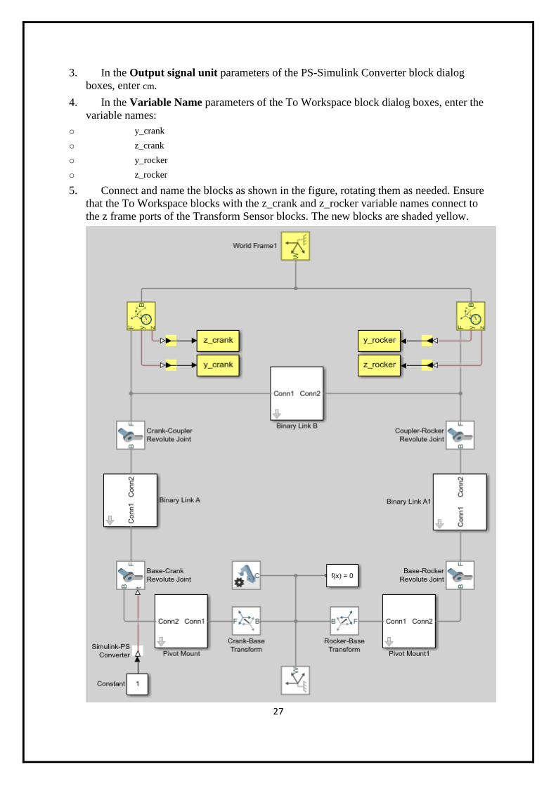
3. In the Output signal unit parameters of the PS-Simulink Converter block dialog

boxes, enter cm.

4. In the Variable Name parameters of the To Workspace block dialog boxes, enter the

variable names:

o y_crank

o z_crank

o y_rocker

o z_rocker

5. Connect and name the blocks as shown in the figure, rotating them as needed. Ensure

that the To Workspace blocks with the z_crank and z_rocker variable names connect to

the z frame ports of the Transform Sensor blocks. The new blocks are shaded yellow.

28

Simulate Model

Run the simulation. You can do this in the Simulink tool bar by clicking the run button.

Mechanics Explorer plays a physics-based animation of the four bar assembly.

Once the simulation ends, you can plot the position coordinates of the coupler link end

frames, e.g., by entering the following code at the MATLAB command line:

figure;

plot(y_crank.data, z_crank.data, 'color', [60 100 175]/255);

hold;

plot(y_rocker.data, z_rocker.data, 'color', [210 120 0]/255);

xlabel('Y Coordinate (cm)');

ylabel('Z Coordinate (cm)');

axis equal; grid on;

The figure shows the plot that opens. This plot shows that the crank completes a full

revolution, while the rocker completes a partial revolution, e.g., it oscillates. This behavior is

characteristic of crank-rocker systems.

29

Simulate Model in Double-Crank Mode

Try simulating the model in double-crank mode. You can change the four-bar linkage into a

double-crank linkage by changing the binary link lengths according to the table.

Block Parameter Value

Binary Link A Length 25

Binary Link B Length 20

Binary Link A1 Length 30

Crank-Base Transform Translation > Offset 5

Rocker-Base Transform Translation > Offset 5

Update and simulate the model. The figure shows the updated visualization display in

Mechanics Explorer.

30

Plot the position coordinates of the coupler link end frames. At the MATLAB command line,

enter:

figure;

plot(y_crank.data, z_crank.data, 'color', [60 100 175]/255);

hold;

plot(y_rocker.data, z_rocker.data, 'color', [210 120 0]/255);

xlabel('Y Coordinate (cm)');

ylabel('Z Coordinate (cm)');

axis equal; grid on;

The figure shows the plot that opens. This plot shows that both links complete a full

revolution. This behavior is characteristic of double-crank linkages.

31

ANALYTICAL SYNTHESIS AND ANALYSIS OF MECHANISMS USING MATLAB AND SIMULINK

%****************

%

%

% Path Generation Program Using Loop Closure Method

%

%

%****************

% FILENAME: path_loop_closure.m

% CREATE MATRICES TO STORE X AND iY COMPONENTS OF POSITION OF PTS.

A,

B,

% AND C AND THETA 3 AND 4 ESTIMATES

Xa=[];

Ya=[];

Xb=[];

Yb=[];

Xc=[];

Yc=[];

thetabars=[];

% DEFINE CONSTANTS (LENGTHS IN INCHES, ANGLES IN RADIANS)

r1=1.178; % "G" Ground Link Length, AoBo

r2=0.3463; % "U" Input Link Length, AoA

r3=1.43; % "Z" Coupler Link Length, AB

r4=1; % "W" Follower Link Length, BoB

r5=1.54; % Length AC

theta1=0; % Angle of Ground Link

psic=40.6*(pi/180); % Angle BAC

mu=-1; % Configuration of linkage

% Grashof (s+l<p+q since r2+r1<r3+r4) and input is the shortest

% link => Crank Rocker (Cranks can rotate 360 degrees)

theta2min=0; % Smallest input angle

theta2max=2*pi; % Largest input angle

range=theta2max-theta2min; % Range of input motion

steps=100; % Number of positions that will be

calculated

% CALCULATE INITIAL POSITION OF C WITH COMPLEX NUMBERS

theta2=theta2min; % Initial theta2

r2v=r2*exp(i*theta2); % Position vector AoA

r1v=r1*exp(i*theta1); % Position vector AoBo

r7v=r2v-r1v; % Position vector BoA

r7=abs(r7v); % Magnitude BoA

psi=acos((r4^2+r7^2-r3^2)/(2*r4*r7)); % Angle ABoB

theta4=imag(log(r7v/abs(r7v)))+mu*psi; % Current theta4

32

r4v=r4*exp(i*theta4); % Position vector BoB

r3v=r1v-r2v+r4v; % Position vector AB

theta3=imag(log(r3v/abs(r3v))); % Angle of AoA to X axis

% CALCULATE POSITION OF C AT ALL STEPS

for q=1:(steps+1)

Page 12.242.11

theta2=theta2min+(q-1)*(range)/steps; % Current theta2

% CALL FUNCTION TO GET ESTIMATES OF THETAS 3 AND 4

thetabars=thetas(theta1,theta2,theta3,theta4,r1,r2,r3,r4);

theta3=thetabars(1); % Set current theta3 to Newton-Raphson

estimate

theta4=thetabars(2); % Set current theta4 to Newton-Raphson

estimate

thth(q)=theta4;

Xc(q)=r2*cos(theta2)+r5*cos(theta3+psic); % Put current Xc in

matrix

Yc(q)=r2*sin(theta2)+r5*sin(theta3+psic); % Put current iYc in

matrix

Xb(q)=r1*cos(theta1)+r4*cos(theta4); % Put current Xb in

matrix

Yb(q)=r1*sin(theta1)+r4*sin(theta4); % Put current iYb in

matrix

Xa(q)=r2*cos(theta2); % Put current Xa in

matrix

Ya(q)=r2*sin(theta2); % Put current iYa in

matrix

end

theta4max=max(thth);

theta4min=min(thth);

range1=(theta4max-theta4min)*180/pi

% PLOT THE POSITIONS OF C, B, AND A

plot(Xc,Yc,Xb,Yb,Xa,Ya);

title('Plot of Positions Using Loop Closure and Newton-Raphson');

axis([-2,4,-2,4]);

xlabel('X Coordinates');

ylabel('iY Coordinates');

legend('Pt. C','Follower- range = 50 degree','Input (Crank)');

animate_nbar

Page 12.242.12

%****************

%

%

%

% Function for Path Generation Program Using Loop Closure Method

% 2-12-06

%

%****************

% FILENAME: thetas.m

% FUNCTION FINDS NEWTON-RAPHSON APPROXIMATION OF THETAS 3 AND 4

33

% BASED ON PREVIOUS ANGLES AND BASED ON LINK MAGNITUDES

function y=thetas(th1,th2,th3,th4,m1,m2,m3,m4)

% SET ESTIMATES EQUAL TO LAST THETAS 3 AND 4

theta3bar=th3;

theta4bar=th4;

%INITIALIZE MATRIX TO STORE X AND Y SUMS

F=[1;1];

% LOOP UNTIL MAGNITUDE OF X AND Y SUMS IS VERY SMALL -- NEAR ZERO

while norm(F)>=1.0e-010 %if eps, program looped forever

% X COMPONENTS AT CURRENT ESTIMATE (MUST ADD UP TO ZERO)

f1=m2*cos(th2)+m3*cos(theta3bar)-m4*cos(theta4bar)-m1*cos(th1);

% Y COMPONENTS AT CURRENT ESTIMATE (MUST ADD UP TO ZERO)

f2=m2*sin(th2)+m3*sin(theta3bar)-m4*sin(theta4bar)-m1*sin(th1);

% JACOBIAN DETERMINATE IS CALCULATED

A=[(-m3*sin(theta3bar)) (m4*sin(theta4bar));(m3*cos(theta3bar))

(-m4*cos(theta4bar))];

%THE X AND Y AT CURRENT ESTIMATE

b=[(-(f1));(-(f2))];

% MATRIX "DIVISION" -- EQUIVALENT TO A^-1*b, BUT FASTER

EXECUTION

x=A\b;

% NEW ESTIMATE OF THETAS 3 AND 4

theta3bar=theta3bar+x(1,1);

theta4bar=theta4bar+x(2,1);

% NEW SUM OF X AND Y COMPONENTS

f1=m2*cos(th2)+m3*cos(theta3bar)-m4*cos(theta4bar)-m1*cos(th1);

f2=m2*sin(th2)+m3*sin(theta3bar)-m4*sin(theta4bar)-m1*sin(th1);

% PUT X AND Y SUMS IN MATRIX SO NORM CAN BE COMPUTED

F=[f1;f2];

end

% FINAL ESTIMATES ARE RETURNED AS A VECTOR

y=[theta3bar theta4bar];

end

34

The MATLAB functions with foreground colors, blue, orange and red, seen in the

SIMULINK model, are MATLAB .m files for finding positions, velocities and accelerations

of the links respectively. The program also animates the mechanism. A snapshot of such an

animation is shown below:

Appendix B contains the three MATLAB Functions used in the SIMULINK model. Figure 5

is the Auto-Scale Graph of the SIMULINK model, which is the plot of the angular position

of link 4 (s4 ) vs. time. Figure 5 confirms the rocking motion of the follower. It also shows

that the follower sweeps an angle of 50o in its rocking motion.

35

Figure 5

Conclusion

The project significantly helped students understand the abstract concepts in dynamics. This

was reflected in the result of the follow up exam. Majority of the students exhibited a very

thorough understanding of Lagrange’s equations. Students enjoyed the animation part of the

project and built their models in the shop. The author received positive feedback from the

students regarding this exercise.

36

ANALYSIS OF KINEMATICS IN FOUR BAR MECHANISM IN MATLAB PROGRAM

%% Plot Any Four Bar Linkage

%% Mohammad Y. Saadeh May, 10, 2010, University of Nevada Las Vegas

clc;clear;close all

X = [150 110 100 90 40 120];

% X = [180 100 185 220 55 0];

% X = [r1 r2 r3 r4 Cx Cy ];

% r1: Crank (make sure its always the smallest, also r3+r4>=r1+r2)

% r2: Coupler

% r3: Lever (Rocker)

% r4: Frame

% Cu: x coordinate for coupler point wrt crank-coupler point

% Cv: y coordinate for coupler point wrt crank-coupler point

cycles = 2;% number of crank rotations

INCREMENTS = 100;% divide a rotation into this number

%% check the geometry

P = X(1:4);

check = P;

[L locL] = max(check);

check(locL) = [];

[S locS] = min(check);

check(locS) = [];

R = check;

flag = 0;

if S==X(4) & sum(check)>(L+S)

TITLE = 'This is a Double-Crank Mechanism';

elseif (S==X(1)|S==X(3)) & sum(check)>(L+S)

TITLE = 'This is a Rocker-Crank Mechanism';

elseif S==X(2) & sum(check)>(L+S)

TITLE = 'This is a Double-Rocker Mechanism';

flag = 1;

elseif sum(check)==(L+S)

TITLE = 'This is a Change Point Mechanism';

elseif sum(check)<(L+S)

flag = 1;

TITLE = 'This is a Double-Rocker Mechanism';

end

%%

TH1 = linspace(0,2*pi,INCREMENTS);% Input angle theta1

dig = 10;% divide links into this number

R1 = X(1); r1 = linspace(0,R1,dig);

R2 = X(2); r2 = linspace(0,R2,dig);

R3 = X(3); r3 = linspace(0,R3,dig);

R4 = X(4); r4 = linspace(0,R4,dig);

Cu = X(5); cu = linspace(0,Cu,dig);

Cv = X(6); cv = linspace(0,Cv,dig);

%% check valid region

D = sqrt(R1^2 + R4^2 - 2*R1*R4*cos(TH1));% diagonal distance between

% crank-coupler point and rocker-frame point

TH5 = acos((R3^2+D.^2-R2^2)./(2*R3*D));% angle between rocker and diagonal

% link (d)

IMAG = imag(TH5);

[VALUES LOCATION] = find(IMAG==0);

%%

IMAG = imag(TH5);

LOCATION = IMAG==0;

LOCATION1 = find(IMAG==0);

LOC = LOCATION;

n = length(LOCATION);

n1 = length(LOCATION1);

37

Check = 0;

direction = 1;

for i=1:n-1

if LOC(i+1)~=LOC(i)

if Check==0

direction = LOC(i);

end

Check = Check+1;

end

end

%%

Rotate = 0;

if isempty(LOCATION1)

error('This is not a valid linkage');

elseif direction==0 & Check==2

LOC1 = find(LOCATION==1);

th1 = [TH1(LOC1) TH1(fliplr(LOC1))];

elseif n1==n

th1 = TH1;

elseif direction==1 & Check==2

Rotate = 1;

loc1 = LOC(1:end-1);

loc2 = LOC(2:end);

[Value deadpoint] = find((loc2-loc1)~=0);

deadp = deadpoint + [0 1];

LOC2 = [deadp(2):n 1:deadp(1)];

th1 = [TH1(LOC2) TH1(fliplr(LOC2))];

elseif Check==4

Rotate = 1;

loc1 = LOC(1:end-1);

loc2 = LOC(2:end);

[Value deadpoint] = find((loc2-loc1)~=0);

deadp1 = deadpoint(1:2) + [1 0];

deadp2 = deadpoint(3:4) + [1 0];

fprintf('This mechanism has two disconnected upper and lower regions\n');

DIREC = 1;

DIREC = input('Select [1] for upper, [2] for lower Default = [1] ');

if DIREC == 1

LOC3 = [deadp1(1):deadp1(2)];

else

LOC3 = [deadp2(1):deadp2(2)];

end

th1 = [TH1(LOC3) TH1(fliplr(LOC3))];

end

d = sqrt(R1^2 + R4^2 - 2*R1*R4*cos(th1));

th5 = acos((R3^2+d.^2-R2^2)./(2*R3*d));% angle between rocker and

%%

if Rotate == 1

d = sqrt(R1^2 + R4^2 - 2*R1*R4*cos(th1));

th5 = acos((R3^2+d.^2-R2^2)./(2*R3*d));% angle between rocker and diagonal link (d)

th5 = [th5(1:end/2) -th5(end/2+1:end)];

end

Ax = R1*cos(th1);% x coordinate for the crank-coupler point

Ay = R1*sin(th1);% y coordinate for the crank-coupler point

a = R4 - R1*cos(th1);% horizontal distance between rocker-frame point and

% projection of crank-coupler point

b = Ay;% vertical projection of crank-coupler point

th6 = atan2(b,a);% angle between frame and diagonal link (d)

th4 = pi - th5 - th6;% angle the rocker makes with horizon

Bx = R3*cos(th4) + R4;% horizontal distance between frame-crank point and

% projection of coupler-rocker point

By = R3*sin(th4);% vertical projection of coupler-rocker point

38

th2 = atan2((By-Ay),(Bx-Ax));% angle the coupler makes with the horizon

Cx = Ax + Cu*cos(th2) - Cv*sin(th2);% horizontal projection of coupler

% point wrt coupler

Cy = Ay + Cu*sin(th2) + Cv*cos(th2);% vertical projection of coupler

% point wrt coupler

% calculate display (figure) limits

xmin = 1.2*min([min(Cx) -R1 -R3]);

xmax = 1.2*max([max(Cx) R4+max([R3 max(R3*cos(th4))])]);

ymin = 1.2*min([min(Cy) -R1 -R3]);

ymax = 1.2*max([max(Cy) max([R1 R3 R3+Cv])]);

%%

increments = length(th1);

for i=1:increments

link1x(i,:) = r1*cos(th1(i));

link1y(i,:) = r1*sin(th1(i));

link2x(i,:) = linspace(Ax(i),Bx(i),dig);

link2y(i,:) = linspace(Ay(i),By(i),dig);

link3x(i,:) = R4 + r3*cos(th4(i));

link3y(i,:) = r3*sin(th4(i));

Couplx1(i,:) = linspace(Ax(i),Cx(i),dig);

Couply1(i,:) = linspace(Ay(i),Cy(i),dig);

Couplx2(i,:) = linspace(Cx(i),Bx(i),dig);

Couply2(i,:) = linspace(Cy(i),By(i),dig);

end

for k=1:cycles

for i = 1:increments

plot(link1x(i,:),link1y(i,:),'b',link2x(i,:),link2y(i,:),'r',...

link3x(i,:),link3y(i,:),'k',Couplx1(i,:),Couply1(i,:),'r',...

Couplx2(i,:),Couply2(i,:),'r')

hold on

plot([link2x(i,:) ;Couplx1(i,:)],[link2y(i,:); Couply1(i,:)],'g','linewidth',2)

plot([link2x(i,:) ;Couplx2(i,:)],[link2y(i,:); Couply2(i,:)],'g','linewidth',2)

plot(0,0,'sk',R4,0,'sk','MarkerSize',12)

plot(0,0,'ok',R4,0,'ok')

plot(Couplx1(i,end),Couply1(i,end),'ok','MarkerSize',6,...

'MarkerFaceColor','g')

axis([xmin xmax ymin ymax])

if Rotate == 1 & i<=increments/2

plot(Couplx1(1:i,end),Couply1(1:i,end),'--g','linewidth',2)

elseif Rotate == 1

plot(Couplx1(1:increments/2,end),Couply1(1:increments/2,end),'--g','linewidth',2)

plot(Couplx1(increments/2:i,end),Couply1(increments/2:i,end),'--r','linewidth',2)

else

plot(Couplx1(1:i,end),Couply1(1:i,end),'--g','linewidth',2)

end

clc

title(['\bf',TITLE])

fprintf('Th1 = %5.2f, th5 = %5.2f, D = %7.2f\n',th1(i),th5(i),d(i))

YY = input('Hit Enter ');

hold off

end

end

if Rotate==1

hold on

plot(Couplx1([1 end/2],end),Couply1([1 end/2],end),'hr','MarkerSize',10)

end

39

WEEK-7

MATLAB PROGRAM FOR EULERS EQUATION OF MOTION

Using the Euler method solve the following differential equation. At x = 0, y = 5.

y' + x/y = 0

Calculate the Numerical solution using step sizes of .5; .1; and .01

From my text book I have coded Euler's method

function [t,y] = eulode(dydt, tspan, y0, h)

%eulode: Euler ODE solver

% [t,y] = eulode(dydt, tspan, y0, h, p1, p2,...)

% ` uses EULER'S method to INTEGRATE an ODE

% (uses the slope at the beginning of the stepsize to graph the

% function.)

%Input:

% dydt = name of hte M-file that evaluates the ODE

% tspan = [ti,tf] where ti and tf = initial and final values of

% independent variables

% y0 = initial value of dependent variable

% h = step size

% p1,p2 = additional parameter used by dydt

%Output:

% t = vector of independent variable

% y = vector of solution for dependent variable

if nargin<4, error('at least 4 input arguments required'), end

ti = tspan(1); tf = tspan(2);

if ~ (tf>ti), error('upper limit must be greater than lower limit'), end

t = (ti:h:tf)';

n = length(t);

%if necessary, add an additional value of t

%so that range goes from t=ti to tf

if t(n)<tf

t(n+1) = tf;

n = n+1;

t(n)=tf;

end

y = y0*ones(n,1); %preallocate y to improve efficiency

for i = 1:n-1 %implement Euler's Method

y(i+1) = y(i) + dydt(t(i),y(i))*(t(i+1)-t(i));

end

plot(t,y)

I have made another m-file to run Eulode, what I am confused with is where do I input my

different step sizes and where do I input x=0 and y=5. However since the analytical solution

yields:

simplify(dsolve('Dy=-x/y','y(0)=5','x'))

ans =

(-x^2+25)^(1/2)

40

and when x=0 the value is 5 so I have coded my Euler's Method like the following and the final

values are close to 5 so I think it is correct can someone just verify.

dydx=@(x,y) -(x/y);

[x1,y1]=eulode(dydx, [0 1],5,.5);

[x2,y2]=eulode(dydx,[0 1],5,.1);

[x3,y3]=eulode(dydx,[0 1],5,.01);

disp([x1,y1])

disp([x2,y2])

disp([x3,y3])

41

WEEK-8

MATLAB PROGRAM FOR CURVE FITTING

Polynomial curve fitting

collapse all in page

Syntax

p = polyfit(x,y,n)

[p,S] = polyfit(x,y,n)

[p,S,mu] = polyfit(x,y,n)

Description

p = polyfit(x,y,n) returns the coefficients for a polynomial p(x) of degree n that is a best fit (in a least-

squares sense) for the data in y. The coefficients in p are in descending powers, and the length

of p is n+1

p(x)=p1xn+p2x

n−1+...+pnx+pn+1.

[p,S] = polyfit(x,y,n) also returns a structure S that can be used as an input to polyval to obtain error estimates.

[p,S,mu] = polyfit(x,y,n) also returns mu, which is a two-element vector with centering and scaling

values. mu(1) is mean(x), and mu(2) is std(x). Using these values, polyfit centers x at zero and scales it to have unit standard deviation,

ˆx=x−

‾xσ

x .

This centering and scaling transformation improves the numerical properties of both the polynomial

and the fitting algorithm.

Examples

collapse all

Fit Polynomial to Trigonometric Function

Try This Example

View MATLAB Command

Generate 10 points equally spaced along a sine curve in the interval [0,4*pi].

x = linspace(0,4*pi,10);

y = sin(x);

Use polyfit to fit a 7th-degree polynomial to the points.

p = polyfit(x,y,7);

Evaluate the polynomial on a finer grid and plot the results.

x1 = linspace(0,4*pi);

y1 = polyval(p,x1);

figure

plot(x,y,'o')

hold on

plot(x1,y1)

42

hold off

Fit Polynomial to Set of Points

Try This Example

View MATLAB Command

Create a vector of 5 equally spaced points in the interval [0,1], and evaluate y(x)=(1+x)−1 at those

points.

x = linspace(0,1,5);

y = 1./(1+x);

Fit a polynomial of degree 4 to the 5 points. In general, for n points, you can fit a polynomial of

degree n-1 to exactly pass through the points.

p = polyfit(x,y,4);

Evaluate the original function and the polynomial fit on a finer grid of points between 0 and 2.

x1 = linspace(0,2);

y1 = 1./(1+x1);

f1 = polyval(p,x1);

Plot the function values and the polynomial fit in the wider interval [0,2], with the points used to

obtain the polynomial fit highlighted as circles. The polynomial fit is good in the

original [0,1] interval, but quickly diverges from the fitted function outside of that interval.

figure

plot(x,y,'o')

hold on

plot(x1,y1)

plot(x1,f1,'r--')

43

legend('y','y1','f1')

Fit Polynomial to Error Function

Try This Example

View MATLAB Command

First generate a vector of x points, equally spaced in the interval [0,2.5], and then evaluate erf(x) at

those points.

x = (0:0.1:2.5)';

y = erf(x);

Determine the coefficients of the approximating polynomial of degree 6.

p = polyfit(x,y,6)

p = 1×7

0.0084 -0.0983 0.4217 -0.7435 0.1471 1.1064 0.0004

To see how good the fit is, evaluate the polynomial at the data points and generate a table showing the

data, fit, and error.

f = polyval(p,x);

T = table(x,y,f,y-f,'VariableNames',{'X','Y','Fit','FitError'})

T=26×4 table

X Y Fit FitError

___ _______ __________ ___________

0 0 0.00044117 -0.00044117

0.1 0.11246 0.11185 0.00060836

44

0.2 0.2227 0.22231 0.00039189

0.3 0.32863 0.32872 -9.7429e-05

0.4 0.42839 0.4288 -0.00040661

0.5 0.5205 0.52093 -0.00042568

0.6 0.60386 0.60408 -0.00022824

0.7 0.6778 0.67775 4.6383e-05

0.8 0.7421 0.74183 0.00026992

0.9 0.79691 0.79654 0.00036515

1 0.8427 0.84238 0.0003164

1.1 0.88021 0.88005 0.00015948

1.2 0.91031 0.91035 -3.9919e-05

1.3 0.93401 0.93422 -0.000211

1.4 0.95229 0.95258 -0.00029933

1.5 0.96611 0.96639 -0.00028097

⋮

In this interval, the interpolated values and the actual values agree fairly closely. Create a plot to show

how outside this interval, the extrapolated values quickly diverge from the actual data.

x1 = (0:0.1:5)';

y1 = erf(x1);

f1 = polyval(p,x1);

figure

plot(x,y,'o')

hold on

plot(x1,y1,'-')

plot(x1,f1,'r--')

axis([0 5 0 2])

hold off

45

Use Centering and Scaling to Improve Numerical Properties

Try This Example

View MATLAB Command

Create a table of population data for the years 1750 - 2000 and plot the data points.

year = (1750:25:2000)';

pop = 1e6*[791 856 978 1050 1262 1544 1650 2532 6122 8170 11560]';

T = table(year, pop)

T=11×2 table

year pop

____ _________

1750 7.91e+08

1775 8.56e+08

1800 9.78e+08

1825 1.05e+09

1850 1.262e+09

1875 1.544e+09

1900 1.65e+09

1925 2.532e+09

1950 6.122e+09

1975 8.17e+09

2000 1.156e+10

plot(year,pop,'o')

46

Use polyfit with three outputs to fit a 5th-degree polynomial using centering and scaling, which

improves the numerical properties of the problem. polyfit centers the data in year at 0 and scales it to

have a standard deviation of 1, which avoids an ill-conditioned Vandermonde matrix in the fit

calculation.

[p,~,mu] = polyfit(T.year, T.pop, 5);

Use polyval with four inputs to evaluate p with the scaled years, (year-mu(1))/mu(2). Plot the results

against the original years.

f = polyval(p,year,[],mu);

hold on

plot(year,f)

hold off

Simple Linear Regression

Try This Example

View MATLAB Command

Fit a simple linear regression model to a set of discrete 2-D data points.

Create a few vectors of sample data points (x,y). Fit a first degree polynomial to the data.

x = 1:50;

y = -0.3*x + 2*randn(1,50);

p = polyfit(x,y,1);

Evaluate the fitted polynomial p at the points in x. Plot the resulting linear regression model with the

data.

f = polyval(p,x);

47

plot(x,y,'o',x,f,'-')

legend('data','linear fit')

Linear Regression With Error Estimate

Try This Example

View MATLAB Command

Fit a linear model to a set of data points and plot the results, including an estimate of a 95% prediction

interval.

Create a few vectors of sample data points (x,y). Use polyfit to fit a first degree polynomial to the data.

Specify two outputs to return the coefficients for the linear fit as well as the error estimation structure.

x = 1:100;

y = -0.3*x + 2*randn(1,100);

[p,S] = polyfit(x,y,1);

Evaluate the first-degree polynomial fit in p at the points in x. Specify the error estimation structure as

the third input so that polyval calculates an estimate of the standard error. The standard error estimate

is returned in delta.

[y_fit,delta] = polyval(p,x,S);

Plot the original data, linear fit, and 95% prediction interval y±2Δ.

plot(x,y,'bo')

hold on

plot(x,y_fit,'r-')

plot(x,y_fit+2*delta,'m--',x,y_fit-2*delta,'m--')

title('Linear Fit of Data with 95% Prediction Interval')

legend('Data','Linear Fit','95% Prediction Interval')

48

49

WEEK-9

DYNAMICS AND VIBRATION ANALYSIS

SOFTWARE REQUIRED

1. MATLAB R2013a.

2. Windows 7/XP SP2.

PROCEDURE

1. Open MATLAB 2. Open new M-file

3. Type the program

4. Save in current directory

5. Compile and Run the program

6. For the output see command window\ Figure window

PROGRAM

A 5 kg block is attached to a cable cable and to a spring as shown in Fig.

The constant of the spring is k = 3 kN/m and the tension in the cable is 30 N.

When the cable is cut,

(a) derive an expression for the velocity of the block as a function of its displacement x, (b) determine the maximum displacement xm and the maximum speed vm, (c) plot the speed of the block as a function of for 0 x xm.

(b) Solution: Free-body diagram of the block before and after the cable is cut is shown in Fig.

For the static case we have entire forces are in equilibrium.

T + R – W = 0 with T =30 N, W = mg = 50 N

from which R = 20 N

50

51

WEEK-10

MATLAB PROGRAM TO PLOT THE RESULTANT ACCELERATION AND THE

VARIATION OF ACCELERATION

52