computational - univ-brest.fr

Enrico Formenti • Roberto TagliaferriErnst Wit (Eds.)

ComputationalIntelligence Methodsfor Bioinformaticsand Biostatistics

10th International Meeting, CIBB 2013Nice, France, June 20–22, 2013Revised Selected Papers

123

French Flag Tracking by MorphogeneticSimulation Under Developmental Constraints

Abdoulaye Sarr(B), Alexandra Fronville, Pascal Ballet, and Vincent Rodin

UMR CNRS 6285, Lab-STICC, CID, IHSEV, Computer Science Department,Universite de Brest, 20 avenue Le Gorgeu, 29200 Brest, France

[email protected]

Abstract. Below the influence of the mechanical cues and genetic expres-sion, constraints underlying the developmental process play a key rolein forms’ emergence. Theses constraints lead to cells’ differentiation andsometimes determine the directions of cells growth. To better under-stand these phenomena, we present in this paper our work focused pri-marily on a development of a mathematical model. A one which takesinto account the co-evolution of cellular dynamics with it’s environment.To study the influence of the developmental constraints, we have devel-oped algorithms to make and explore a base of genomes. The purposeof this exploration is first to check conditions under which specific genesare activated. Then, this exploration allows us to follow the conditionsof emergence of some patterns that lead to a specific shape. From ourmodel, we found a genome that can generate the French flag. With thisFrench flag pattern and its genome starting, we addressed the followingquestion: is there another genome in the simulated base that achievesthe same shape, i.e. the French flag pattern?

Keywords: Mathematical modelling · Simulation of biological systems ·Morphogenesis · Multi-agent system · French flag problem

1 Introduction

1.1 Morphogenesis: Emerging of Interests

Biomedical science has undergone a remarkable evolution during this last decade.Advances and innovations in biotechnology, more particularly in microscopy andimaging, have provided a large amount of data. And these data include all levelsof the biological organization. In 2007, Melani and al. achieved a tracking ofcell’s nuclei and the identification of cell’s divisions in live zebrafish’s embryos.They used 3D+time images acquired by confocal laser scanning microscopy [13].These kind of data allowed new description in details of many components andstructures of living organisms. Observations noticed from these data like geo-metrical segmentations during cells’ proliferation have raised relevant issues inmathematical and numerical point of view. But experimental complexity usu-ally restricts observations to a single or very restricted spatial or temporal scales.c© Springer International Publishing Switzerland 2014E. Formenti et al. (Eds.): CIBB 2013, LNBI 8452, pp. 90–106, 2014.DOI: 10.1007/978-3-319-09042-9 7

French Flag Tracking by Morphogenetic Simulation 91

Thus, one of the purposes of mathematical and computational models in biologyis to reconstruct integrated models from this large amount of data gathered atdifferent scales. So that, the dynamical interactions between different levels ofthe biological organization is taken into account. In cellular proliferation mod-els, it means to consider the cell as a place of integration of causalities anddowngrades.

For this purpose, tensegrity model considers biomechanical forces betweencells and the extracellular matrix. The stretching of cells adhering to the extra-cellular matrix may result from local reshuffle in this latter. According to thismodel, growth-generated strains and pressures in developing tissues regulatemorphogenesis throughout development [9]. It is therefore the biomechanicalforces which play a key role in this model of morphogenesis. For example bymodulating cell’s differentiation, influencing the direction of division or deform-ing tissues. However, the question of cells’ diversity even arises before the acqui-sition of shape [16]. Indeed, when the embryo has only a few pairs of cells, wecan already see a diversification of biochemical content or a diversification ofembryonic cells’ morphology. That may be the result of genetic and molecularinteractions. Indeed, the emergence of shapes also stems from the acquisitionof differential properties, from cells’ mobility and genes’ expression throughouttheir development.

Moreover, Artificial Regulatory Networks also allow modelling morphogene-sis [15]. They define a series of regulatory genes and structural genes. The firstconsist of a network of rules determining the evolution of the system. And thelatter are intended to each generate a simple specific pattern. They can be seenas a dynamical system following different trajectories in a state space [10]. How-ever, even if the detailed knowledge of genomic sequences allows to determinewhere and when different genes are expressed in the embryo, it is insufficient tounderstand how the organism emerge [14].

1.2 Below Genetic Expression

So, we have looked forward to learn more about the emergent properties ofcellular organization. And especially, the importance of cellular dynamics in theemergence and evolution of shapes, both in mathematical and numerical pointof view.

A Multicellular organism is a complex system which can be defined as acomposition of a significant number of elements interacting locally to produce aglobal behaviour. Complex systems are also characterized by a high capacity ofself-adaptation and self-organization similarly to multicellular organisms. Theycan evolve and learn through feedbacks between their external environment andtheir internal architecture. And according to Doursat [5], whether inanimatestructures or living organisms, all processes of shape’s emergence are instancesof decentralized morphological self-organization. When cells evolve, they modifytheir organism which in its turn impacts their behaviour. This is what biologistsmean by co-evolution. Epigenetic considers that this coupling between organismand environment can not be ignored in understanding the development of livingorganisms [19].

92 A. Sarr et al.

In mathematics, the viability theory [2] offers concepts and methods to controla dynamical system in a given fixed environment, in order to maintain it in a setof constraints of viability. Applied to morphogenesis, this means that we shouldhave at least one co-viable evolution of the cells’ state and their environmentbased on each state-environment pair. This formalization allows us to establishfeedback rules in terms of changes in growth direction and cells’ differentiation.This mathematical model was formalized in [7]. So, in our computational model,every cell has its own rules monitored by a set of controls and stays aware ofits neighbourhood. This ensures cells to be autonomous while being aware of awrong evolution of their dynamic, and consequently, to know when to implementfeedback mechanisms. The integration of the behaviours of each component ofthe system allows to determine its global state in a finite time.

In this paper, we are going first to establish the mathematical formalizationof the model described above (Sect. 2) before presenting our morphogenesis simu-lation tool (Sect. 3). Then, we aim to better understand the influences of shape’semergence on cellular dynamics. To do so, we have developed here original algo-rithms based on the mathematical model. The main goal of these algorithms isto explore and simulate a base formed by all possible genomes from a same set ofgenes. Genome and gene don’t have the same meaning here as in Biology. In ourview, a gene carries a set of properties for the cell, such as colour, reproductiveage, energies’ minimum levels, viscosity, rigidity, maximum allowable pressure,tolerated stress threshold, choice of dividing direction etc. In a given simulation,it’s allowable to not define some of theses properties. Genes are designated bytheir index. A genome is defined as a suit of genes’ indexes. During a simulation,when a gene in a genome is activated, cells adopt the properties defined by thisgene. The exploration of the base of genomes allows us to verify the conditionsunder which certain genes are activated. And more specifically, if these condi-tions are unique for a targeted pattern (Sect. 4). We test the algorithms on ourmorphogenesis simulation tool with the French flag as being the form to reach(Sect. 5). Finally, we conclude before highlighting some relevant applications andfuture prospects we could give to them (Sect. 6).

2 Morphological Dynamic of Cells

2.1 Mathematical Model

We proposed in [7] a mathematical model of morphogenesis through a formaliza-tion of cellular dynamics in the context of mutational and morphological analysis[1,12]. It provides an extension of differential equations in a metric space insteadof the classical Euclidean space RN . At the tissue level, we have a large groupof connected cells, of a same cellular type, performing a specific function [18].Therefore, the behaviour of cellular tissue can be seen as a result of a bottom-upprocess of cellular dynamic. A minor change on tissue implies that cells haveimplemented dynamics where each cell can not only “move” but also can multi-ply, die or stay quiescent (see Fig. 1).


Fig. 1. Multivalued analysis to formalize a cell that multiplies and moves

M ⊂ R3 denotes the cells’ containment and represents the complement of thevitellus1.

K ⊂ R3 representing tissue cells, the cells are denoted by x ∈ K ⊂ R3.If we restrict morphogenesis in the plan,

D := {(1, 0), (−1.0)(0, 1), (0,−1)}

For convenience, we note:D := {1, 3, 2, 4}

denotes the set of 4 planes directions and

D := D ∪ {(0, 0)} ∪ ∅

means the 6 “extended” directions.For morphogenesis in the space R3,

D := {(1, 0, 0), (−1, 0, 0), (0, 1, 0), (0,−1, 0), (0, 0, 1), (0, 0, −1)}

For convenience:D := {1, 3, 2, 4, 5, 6}

denotes the set of six directions and D := D ∪ {(0, 0, 0)} ∪ ∅ means the eight“extended” directions.We note

ΞM (K,x) := {u ∈ D, such that x + u ∈ {x} ∪ (M \ K)}

andRM (K,x) := ΞM (K,x) × ΞM (K,x).

Then we introduce the correspondence

Ψ(x, u, v) := {x + u} ∪ {x + v}(u,v)∈RM (K,x).

The morphological dynamic ΦM is then defined by

ΦM (K) :=⋃

x∈K

⋃

(u,v)∈RM (K,x)

Ψ(x, u, v) (1)

And the discrete morphological dynamic Kn+1 = ΦM (Kn).1 In biology, the vitellus is the energy reserve used by the embryo during its

development.

94 A. Sarr et al.

This gives the different cases of cell behaviour:

1. apoptosis, obtained by taking (∅, ∅) ∈ RM (K,x) since Ψ(x, ∅, ∅) = ∅ ∪ ∅ = ∅2. migration by taking u ∈ D and v = ∅ or u = ∅ and v ∈ D or further u = v3. stationarity, which is a migration obtained by taking u and v equal to (0, 0, 0)4. cell division by taking u := (0, 0, 0) and v ∈ ΞM (K,x) (or vice-versa)5. division and migration by taking u ∈ ΞM (K,x) and v ∈ ΞM (K,x)

We introduce an equivalence relation on the directions

u ≡x v if and only if x + u = x + v

which we denote by µ and ν the representatives, noting that by construction,for every pair (µ, ν) the equivalence class, for all u ∈ µ and v ∈ ν, Ψ(x, µ, ν) =Ψ(x, u, v) does not depend on the choice of directions belonging to equivalenceclasses.

Because two cells can not occupy the same position, at most they just selectone extensive direction in each class.

The correspondence of regulation is defined by the quotient set:

ΘM (K,x) := RM (K,x)/ ≡x (2)

The morphological dynamics ΦM is always defined by

ΦM (K) :=⋃

x∈K

⋃

(µ,ν))∈ΘM (K,x)

Ψ(x, µ, ν)

=⋃

x∈K

⋃

(u,v)∈∈RM (K,x)

Ψ(x, u, v)(3)

In the case of a discrete dynamic, it is defined by the sequences of control (un, vn)associated to Kn to be able to define K(n+1).

Implementing this formalization is to set the viable directions throughoutthe developmental process whatever underlying constraints.

2.2 Shapes Emergence

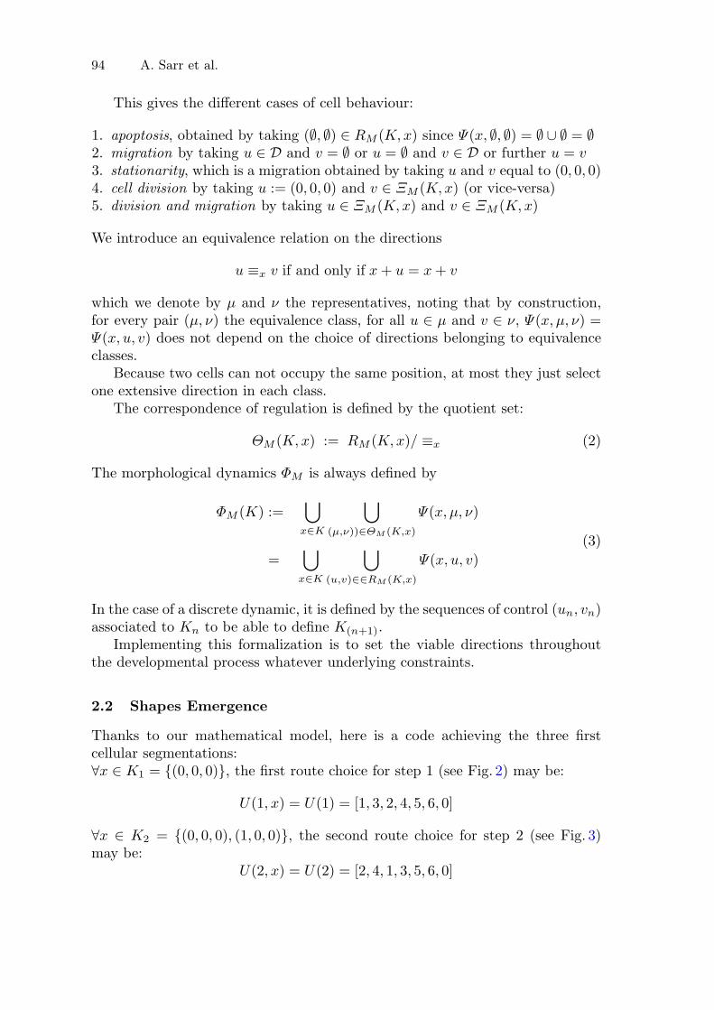
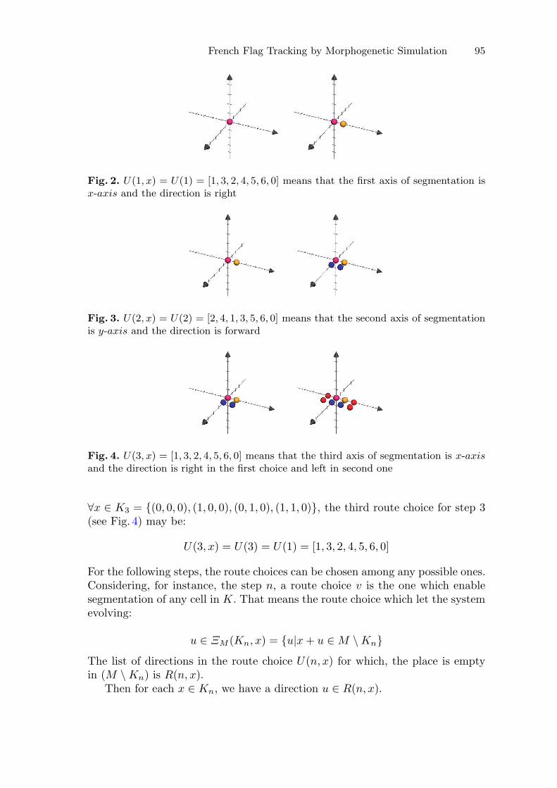
Thanks to our mathematical model, here is a code achieving the three firstcellular segmentations:∀x ∈ K1 = {(0, 0, 0)}, the first route choice for step 1 (see Fig. 2) may be:

U(1, x) = U(1) = [1, 3, 2, 4, 5, 6, 0]

∀x ∈ K2 = {(0, 0, 0), (1, 0, 0)}, the second route choice for step 2 (see Fig. 3)may be:

U(2, x) = U(2) = [2, 4, 1, 3, 5, 6, 0]


Fig. 2. U(1, x) = U(1) = [1, 3, 2, 4, 5, 6, 0] means that the first axis of segmentation isx-axis and the direction is right

Fig. 3. U(2, x) = U(2) = [2, 4, 1, 3, 5, 6, 0] means that the second axis of segmentationis y-axis and the direction is forward

Fig. 4. U(3, x) = [1, 3, 2, 4, 5, 6, 0] means that the third axis of segmentation is x-axisand the direction is right in the first choice and left in second one

∀x ∈ K3 = {(0, 0, 0), (1, 0, 0), (0, 1, 0), (1, 1, 0)}, the third route choice for step 3(see Fig. 4) may be:

U(3, x) = U(3) = U(1) = [1, 3, 2, 4, 5, 6, 0]

For the following steps, the route choices can be chosen among any possible ones.Considering, for instance, the step n, a route choice v is the one which enablesegmentation of any cell in K. That means the route choice which let the systemevolving:

u ∈ ΞM (Kn, x) = {u|x + u ∈ M \ Kn}

The list of directions in the route choice U(n, x) for which, the place is emptyin (M \ Kn) is R(n, x).

Then for each x ∈ Kn, we have a direction u ∈ R(n, x).

96 A. Sarr et al.

And ψ(x, 0, u) = {x} ∪ {x + u}

Kn+1 = ΦM (Kn) =⋃

x ∈ Kn

u ∈ R(n, x)

Ψ(x, u)

=⋃

x∈Kn

Ψ(x,R(n, x))

3 Simulation Tool

In this section, we describe Dyncell which is a tool developed for simulatinggenerative systems [6]. The platform was created to experiment our theoreticalmodel of morphogenesis.

The program is implemented in C++ using a tool kit of Virtual Reality: AReVi[4,17]. AReVi is a simulation library of autonomous entities with a 3D renderingdeveloped at European Center of Virtual Reality (Brest, France).

3.1 Architecture

The architecture of our simulation tool is based on the concept of shape. Allclasses inherit from a generic parent class called Form (see Fig. 5). During simu-lation, each instantiated object is a form by definition.

Fig. 5. Dyncell classes diagram


This class has two main subclasses: Environment and Cell, which are thetwo types of objects to be instantiated before starting any simulation.

Running a simulation always consists of instantiating an object Environmentand some Cells objects evolving in this environment.

Class Cell is responsible for representing cells. Then, an object Cell isdefined by its age, color, division speed and energy amount. During mitosis,another Cell object is created next to the mother Cell object that triggeredthe division. The position of the daughter Cell depends on the route choicetaken by its mother, as defined in the mathematical model.

Environment is a Form object which has a lifetime. It is used to delimit thespace in which cells’ population operates or to exert external forces on them.

3.2 Features

The order of scheduling has a significant impact on the results of the simulation[3,11]. It determines how local interactions (self-organization) have been held.Thus, how and when the system reaches the final shape. Different behaviourscan be observed in virtual models depending on the scheduling mode. Whenmodelling natural systems, asynchronism seems more appropriate. In morpho-genesis, for instance, synchrony is likely to cause false correlations between cells.In AReVi, scheduling of agents is handled implicitly in asynchronous and stochas-tic way. Routines of each agent are executed sequentially and entirely, the samenumber of times. However the running order of agents is randomly determined.We set as a basic principle that cells are autonomous agents and ignorant of thewhole system even if they can perceive their environment and adapt accordingly.They are represented on screen by spheres and can proliferate in a discrete envi-ronment (cellular automaton) or in a “continuous” one. In the latter case, themovement of cells is more precisely described and we can have more complexinteractions.

A graphical interface has been implemented in order to set the options of thesimulation. It allows dynamic change of parameters and selecting mechanisms(e.g. apoptosis) that will be active/inactive during the simulation.

Options are available to allow choice between 2D/3D, discrete or continuoussimulations. The size and shape of both the environment and the cells can alsobe defined and adjusted.

Spatial constraints are crucial for evolution of the cells. If they are too heavy,the cell is not viable as it can no longer divide. A maximal constraint parametersets up a threshold below which the cell can remain viable.

To account for the influence of the environment, a parameter is defined as themaximum number of cells that a cell is able to push when it divides. When thecurrent strain of the cell is greater than the maximum stress threshold, the cellcan no longer divide. To stay alive, a cell can undertake two modes of mitosis.Firstly, the cell chooses to divide in the direction where the stress is less intense.Secondly, it takes a predetermined direction.

It is also possible to assign an amount of energy to each Cell. The basicidea is to consider that an organism accumulates a certain reserve of energy by

98 A. Sarr et al.

consuming its environment’s foods. A percentage of this reserve is used to main-tain its structure and growth. The remaining part is used for its maturation andreproduction. Thus, in Dyncell, at each timestep, cells lose an energy amountintended for their structure maintaining. Moreover, during mitosis, the energylevel is shared between the mother and the daughter Cell. A Cell dies when itsenergy level becomes too low.

4 Algorithms

At the initial stage of living organisms’ creation, all cells have the same genome.But during the developmental process, they don’t all express the same genes.Why has the dynamic of these cells changed to lead to their differentiation?What are the factors that come into play? What is the mechanism by which thistakes place?

These are the questions that underlie any understanding of collective self-organization and self-adaptation mechanisms that target then achieve the well-guided form of living organisms. To address them, it is important to considerthe influence of the developmental process on the overall shape. Besides, theunderlying constraints that this development imposes locally to the cells mustbe considered. The idea of the algorithms we have developed to study this influ-ence is greatly inspired by the concept that Waddington introduced in 1940 asthe epigenetic landscape [20]. The barriers through this landscape are similar tothe constraints that the form faces through its development. Thus, each possiblepath of the landscape represents a possible form evolution process. In fact, anevolution is held in given conditions where only some specific genes can be acti-vated (see Fig. 6). The identification of the obstacles across the landscape allowsto know where and when feedback mechanisms are involved (i.e. differentiationthat gives a particular character to the form at this time).

To study the effect of the developmental process constraints, we verify theconditions under which feedback mechanisms are triggered. To do so, we have

Fig. 6. In 1957, Conrad Waddington proposed the concept of an epigenetic landscapeto represent the process of cellular decision-making during development. At variouspoints in this dynamic visual metaphor, the cell (represented by a ball) can take specificpermitted trajectories, leading to different outcomes or cell fates [8].


generated a base of genomes formed from the same set of genes. Having a genomethat achieves a given shape, we aim to explore the entire space of possiblegenomes. The aim is to see if we can find another genome which allows to reach it.

In this paper we have chosen to target the well known French flag. Thatmeans we have sought genomes that give forms with these followingcharacteristics:

– activation of the same genes as the French flag (same colors),– choice of same segmentation directions as the French flag (same shape).

In Waddington’s point of view, it implies that from different origins on thetop of the epigenetic landscape, the ball can go through different trajectories andfinally hits the same endpoint.

4.1 Software Architecture

In our software architecture, we have two main classes which handle explorationand simulation activities.

1. Genome: represents a genome and allows us to manage all treatments that canbe performed on a genome. As we designed it, a genome is composed of oneor more genes that are activated or not during the simulation.

2. GenerateGenome: includesall theactivitiesofexploration, initialization, launch-ing and stop. It carries initialization of the exploration’s parameters methods,start and stop genome’s simulation methods, genomes’ treatments methods, setof genomes’ managing methods, exploration results’ recording methods.

4.2 Genomes Base Construct

Genes are defined in an xml file with all their attributes (coded color, appliedroute choice, number of repetitions in the genome, etc.). From this file, they areloaded into a vector. And from this vector, we create all possible combinationsof genomes. Their construction is based on the characteristics of the French flaggenome which are:

1. must be composed of 4 genes2. the 1st gene in the genome must be the same as the 4th gene3. if n is the number of times in which is repeated the 1st gene in the genome

(called multiplicity of the gene), the 2nd gene must have therefore a multi-plicity of 2xn and n for the 3rd and 4th genes.

Thus, all genomes are constructed in the same way (see Table 1).

100 A. Sarr et al.

Table 1. French Flag genome characteristics

Genes Gene 1 Gene 2 Gene 3 Gene 1

Multiplicity n 2xn n n

Table 2. French Flag genome simulation results

Multiplicity Number of cells Age

3 70 1.16

4 117 1.224

5 176 1.288

6 247 1.352

4.3 Initialization

During initialization, we define matching criteria to be achieved by simulatedgenomes in the base. When simulating French flag genome, we chose 3 as thefirst gene’s order of multiplicity. We note that the multiplicity doesn’t affect theshape but just its size. The bigger it is, the larger is the shape. And 3 is anoptimal value for an exploration of such a large base.

In Table 2, we have some informations from different simulations performedwith French flag genome. For a given multiplicity of the French flag’s genome(row 1), we have the values of the criteria recorded during the simulation. Thenumber of cells that make it up (row 2) and the age at which it reaches itsfinal form (row 3). The current time is determined during the simulation by thescheduler and is expressed as a double.

So, during the exploration, to assess that a given genome has achieved theFrench flag, we mainly refer to these values of these criteria.

4.4 Description of the Algorithm

The goal of the algorithm is to explore all genomes. Each one is simulated inorder to check if it is able to reach the French flag. In other terms, if it canachieve the same number of cells as the French flag in an identical time. If asuch genome is found, the algorithm lists it as well as the order of multiplicitywith which it has converged.

Outside a match, there may be two cases (see Fig. 7):

1. the number of cells exceeds that corresponding to the current choice of multi-plicity. So we definitely assume that we can’t reach the French flag with thisgenome. In this case, the algorithm continues exploring and pick its followerin the base.

2. the number of cells doesn’t reach that of the current choice of multiplicity.So, the algorithm reloads and simulates the same genome, but leads it to ahigher order of multiplicity (i.e. from 3 to 4). In the 2nd simulation of the


Fig. 7. The algorithm’s flowchart

genome, if the number of cells corresponding to this new choice of multiplicityis met, then the genome is finally listed. Else, if the number of cells exceeds,we execute the same treatment as in (1). Else, if during this second simulationof the genome, the corresponding number of cells is still not reached, we goback to (2): increase multiplicity from 4 to 5 in the 3rd simulation of thegenome.

While the number of cells keeps being lower than that expected, we rede-fine the current genome by modifying its genes’ parameters of multiplicity. Thisoperation is repeated a maximum allowed number of times. In the algorithm,it is 3 times. So the last choice of multiplicity is 6 with an expected number ofcell of 247 in 1.352 time units. In this step, the genome is no longer reloaded,considered definitely not able to achieve the French flag. Then, the algorithmcontinues exploring and picks its follower in the base.

When the algorithm has finished simulating all genomes, the program stopsand we retrieve the results in an output file.

5 Evaluation

5.1 Test Conditions

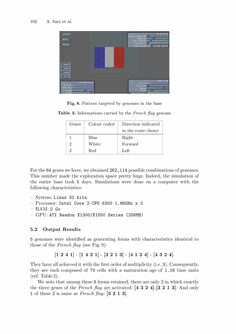
In the tests we have achieved, the targeted pattern was, as shown in Fig. 8, theFrench flag introduced by L. Wolpert in 1969 [21].

The genome which allows to generate the French flag is as follows (details inTable 3): [1 2 3 1].

102 A. Sarr et al.

Fig. 8. Pattern targeted by genomes in the base

Table 3. Informations carried by the French flag genome

Genes Colour coded Direction indicated

in the route choice

1 Blue Right

2 White Forward

3 Red Left

For the 64 genes we have, we obtained 262,114 possible combinations of genomes.This number made the exploration space pretty huge. Indeed, the simulation ofthe entire base took 5 days. Simulations were done on a computer with thefollowing characteristics:

– System: Linux 32 bits– Processor: Intel Core 2 CPU 6300 1.86GHz x 2– RAM: 2 Go– GPU: ATI Readon X1300/X1550 Series (256MB)

5.2 Output Results

5 genomes were identified as generating forms with characteristics identical tothose of the French flag (see Fig. 9):

[1 2 4 1] - [1 4 2 1] - [3 2 1 3] - [4 1 2 4] - [4 3 2 4].

They have all achieved it with the first order of multiplicity (i.e. 3). Consequently,they are each composed of 70 cells with a maturation age of 1.16 time units(ref. Table 2).

We note that among these 5 forms retained, there are only 2 in which exactlythe three genes of the French flag are activated: [4 3 2 4]-[3 2 1 3]. And only1 of these 2 is same as French flag : [3 2 1 3].


Fig. 9. Forms identified by the algorithm that have met matching criteria of the Frenchflag

Fig. 10. Example of a discarded form after three attempts of reaching the French flag

So, from two different genomes, we have reached the same form.Two generated forms discarded by the algorithm are presented in Figs. 10

and 11.The first one presents the case where removal is due to the fact that the

algorithm has reloaded the 3 times authorized the same genome [1 1 3 1] withoutreaching the sought pattern. Based on the output results of the simulation, wecan point out that for these 3 times, the number of cells remains 13. Then, thealgorithm moves to the next genome.

The second one presents the case where removal is due to the exceed numberof cells in the generating form. An excess relative to that of the sought patternwith respect to the defined order of multiplicity. Here too, output results showthat the algorithm aborts the simulation of the genome [3 2 12 3] and proceedsto the next one in the base.

104 A. Sarr et al.

Fig. 11. Example of a discarded form with a number of cells exceeded that targeted

6 Conclusion

Inspired by the concept of epigenetic landscape, we have shown the importance ofthe developmental process constraints on the final form. Starting from 2 differentgenomes, we have achieved the same form thanks to the choices of feedbackmechanisms to deal with stress throughout development. Theses mechanismsare, on the one hand, cellular differentiation. It allows the activated genes toencode the colors of the form. On the other hand, feedback mechanisms implysuccessive changes of direction. This allows to generate (to design) the shape asit goes along.

6.1 Relevance to Biological Issues

The model is tested in French flag pattern because it is a widely known issue instudying the factors that put into play in cells’ differentiation. It constitutes thefirst steps towards the comprehension of biological mechanisms. Nevertheless,in future works, it might be also possible to test the model in real case. Forexample, in genetics, single nucleotide polymorphism (SNP) is the variation of asingle base pair of the genome between individuals of same species. They are usedfor recognition of individuals or reconstruction of family trees. In our algorithm,we could build the genomes’ base so that they are all identical except the lastgene in each of them. This gene, different from one genome to another, wouldconstitute our SNP. Then, to study the influence of this SNP, we can simulatethe genomes and compare the generated forms.

We can also consider applying the algorithm to look for genomes that cangenerate more complex forms. Indeed, from the cell lineage of an organism, we


can know its number of cells and its different type of cells. We can take the case ofCaenorhabditis Elegans (C. Elegans). This is an eukaryote2, which means that itshares cellular structures, molecular structures and control channels with organ-isms of higher species. Thus, its biological informations (embryogenesis, morpho-genesis, growth, etc.) could be directly applicable to more complex organisms,such as humans. In addition, it has a fixed number of cells. The adult her-maphrodite is composed of 959 somatic nuclei and the adult male of 1031 whilethe young consists of 1090. The algorithm can be used to search in the base agenome which can generate a form with the following characteristics: an identi-cal number of cells as the C. Elegans and the same number of activated genesthan cellular types in C. Elegans.

6.2 Future Works

To consider the description of all types of dynamics, we plan to study a gener-alization of our mathematical model. In the current model, when a cell initiatesmitosis, we just create next to it another one. The mother cell does not imple-ment any other mechanism. Therefore, we will consider a mathematical modelwhere the mother cell can in each time step:

– remain quiescent as it is in the current model,– migrate to another point or,– die.

This formalization will allow to reach all possible forms. The development of asuch model raises new challenges in mathematical and numerical perspectives.Because describing all possible dynamics for each cell at each time step offersmany options to consider. In computing, parallel programming on GPU3 couldovercome scalability and duration of simulations.

References

1. Aubin, J.: Mutational and Morphological Analysis: Tools for Shape Regulation andMorphogenesis. Birkhauser, Boston (2000)

2. Aubin, J.-P.: Viability Theory. Birkhauser, Boston (1991)3. Chevaillier, P., Bonneaud, S., Desmeulles, G., Redou, P.: Experimental study of

agent population models with a specific attention to the discretization biases.In: Proceedings of the European Simulation and Modelling Conference (ESM’09),Leicester, UK, pp. 323–331 (2009)

4. Desmeulles, G., Querrec, G., Redou, P., Misery, L., Rodin, V., Tisseau, J.: Thevirtual reality applied to the biology understanding: the in virtuo experimentation.Expert Syst. Appl. 30(1), 82–92 (2006)

2 A eukaryote is an organism whose cells contain complex structures enclosed withinmembranes.

3 Graphics Processing Unit.

106 A. Sarr et al.

5. Doursat, R.: Organically grown architectures: creating decentralized, autonomoussystems by embryomorphic engineering. In: Wurtz, R.P. (ed.) Organic Computing.Springer, Heidelberg (2008)

6. Fronville, A., Harrouet, F., Desilles, A., De Loor, P.: Simulation tool for mor-phological analysis. In: Proceedings of the European Simulation and ModellingConference (ESM’2010), Hasselt, Belgium, pp. 127–132 (2010)

7. Fronville, A., Sarr, A., Ballet, P., Rodin, V.: Mutational analysis-inspired algo-rithms for cells self-organization towards a dynamic under viability constraints.In: SASO 2012, 6th IEEE International Conference on Self-Adaptive and Self-Organizing Systems, Lyon, France, pp. 181–186 (2012)

8. Goldberg, A.D., Allis, C.D., Bernstein, E.: Epigenetics: a landscape takes shape.Cell 128, 635–638 (2007)

9. Henderson, J., Carter, D.: Mechanical induction in limb morphogenesis: the roleof growth-generated strains and pressures. Bone 31(6), 645–653 (2002)

10. Kauffman, S.: The Origins of Order: Self-Organization and Selection in Evolution.Oxford University Press, New York (1993)

11. Lawson, B., Park, S.: Asynchronous time evolution in an artificial society mode.J. Artif. Soc. Soc. Simul. 3(1) (2000)

12. Lorenz, T.: Mutational Analysis - A Joint Framework for Cauchy Problems In andBeyond Vector Spaces. Springer, Berlin (2010)

13. Melani, C., Peyrieras, N., Mikula, K., Zanella, C., Campana, M., Rizzi, B.,Veronesi, F., Sarti, A., Lombardot, B., Bourgine, P.: Cells tracking in the livezebrafish embryo. Conf. Proc. IEEE Eng. Med. Biol. Soc. 1, 1631–1634 (2007)

14. Muller, G., Newman, S.: Origination of Organismal Form: Beyond the Gene inDevelopmental and Evolutionary Biology. MIT Press, Cambridge (2003)

15. Pena, A.C.: Un modele de developpement artificiel pour la generation de structurescellulaires. Ph.D. thesis, Universite de Toulouse, decembre 2007

16. Peyrieras, N.: Morphogenese : L’origine des formes, chapter Morphogenese animale,pp. 179–201. Belin, Paris (2006)

17. Reignier, P., Harrouet, F., Morvan, S., Tisseau, J., Duval, T.: AReVi: a virtualreality multi-agent platform. In: Heudin, J.-C. (ed.) Virtual Worlds 98. LNCS(LNAI), vol. 1434, pp. 229–240. Springer, Heidelberg (1998)

18. Southern, J., Pitt-Francisb, J., Whiteleyb, J., Stokeleyc, D., Kobashid, H.,Nobesa, R., Kadookad, Y., Gavaghan, D.: Multi-scale computational modellingin biology and physiology. Prog. Biophys. Mol. Biol. 96(9), 60–89 (2008)

19. Varela, F.: Principles of Biological Autonomy. North- Holland, New York (1979)20. Waddington, C.: Organisers and Genes. CambridgeUniversity Press, Cambridge

(1940)21. Wolpert, L.: Positional information and the spatial pattern of cellular differentia-

tion. J. Theor. Biol. 25, 1–47 (1969)

computational - univ-brest.fr

Documents