computational vision u. minn. psy 5036 daniel kersten lecture 2: limits...

Computational VisionU. Minn. Psy 5036Daniel KerstenLecture 2: Limits to Vision

Introduction

Last timeThe previous lecture provided an overview of we are going and the approach. To use Marr’s phrase, we'd like to understand how we "know what is where just by looking", how our brains enable us to infer "states of the world", such as scene and object parameters, and how vision supports useful actions.

How to get there? We saw the need for an interdisciplinary approach, and analysis at several different levels of analysis. At the top is a description of behavioral requirements or computational goal. At a lower level, we need to study how to represent the input (image) and output (actions, such as an reach-ing or a decision), and the algorithm to get from input to output. At the lowest level is the study of the neural mechanisms that implement the algorithm to produce a useful behavior.

Computational theory provides a level of analysis at the top and middle levels that can produce a quantitative account of behavior, and helps to bridge our understanding of how the neural mechanisms of vision enable that behavior. Computational theory enables us to specify a procedure (or procedures) to obtain quantitative solutions for estimating "scenes" or "states of the world" S from image input information I. From there we can relate this knowledge to empirical measures of human behavior and underlying neural processes. We saw that the same object can give rise to an infinite variety of images, and a given image could potentially have come from an infinite variety of objects. The visual system must have mechanisms to deal with this uncertainty.

Preview and motivationTo make the problem concrete, think of an object property, say the shape of a face. What do we mean by “shape”? We’ll return to this later in the course, but for the moment assume that “shape” is a geometri-cal description, like a contour depth map. As we saw in the last lecture, intensities are not related to shape in any simple fashion. In fact, we could say that the shape is a signal which is encrypted in the image.

The problem is further compounded by unwanted sources of variation in image intensities. Suppose you are told that the image of a shape could belong to one of two people. The image of a face is light intensity, I(x,y), where (x,y) are coordinates in retinal space. The image can also vary because of differing lighting conditions N = {illumination1, illumination 2, ...}. If you are trying to recognize the face, these variations in illumination are like "noise" in the sense that these variables confound the causes of the intensity patterns, and thus interfere with signal estimation. So the image is an encrypted and noisy function (f) of the shape signal:

I(x,y) = f(shape S, illumination N). The goal is to recover the signal as best we can. Call the recovered signal S'.

The problem is further compounded by unwanted sources of variation in image intensities. Suppose you are told that the image of a shape could belong to one of two people. The image of a face is light intensity, I(x,y), where (x,y) are coordinates in retinal space. The image can also vary because of differing lighting conditions N = {illumination1, illumination 2, ...}. If you are trying to recognize the face, these variations in illumination are like "noise" in the sense that these variables confound the causes of the intensity patterns, and thus interfere with signal estimation. So the image is an encrypted and noisy function (f) of the shape signal:

I(x,y) = f(shape S, illumination N). The goal is to recover the signal as best we can. Call the recovered signal S'.

This example shows that modelling how image information is generated, i.e. characterizing the "generative model", could be a first step towards understanding the inference problem. The example also suggests that we might get some mileage from thinking about the computational problem in terms of "communication"--image measurements I contain information about a signal S that the world is "sending" us (e.g. scene variable such as object shape, size, or material property) but the signal is encrypted and muddled by unwanted, unknown, variability N. This kind of problem has been studied a lot over the past sixty years or so by communication engineers and psychologists, and is called the Signal Detection Theory (SDT).

In general, your eye's retinal image of a signal (say your friend's face) is never the same from one time to the next because of changes in illumination, viewpoint, makeup, hair, or even age. But this is very complicated to analyze, so let's start off with the much simpler case of variability in the intensity of a single spot of light.

VariabilityImagine you have a flashlight with a high and low beam setting, and you want to send a signal (S = high or low) to a distant friend by flashing a light with either the high or the low beam on (e.g. "high if by land, and low if by sea"). In a perfect world, this would be a one bit communication system. But the world isn't perfect and suppose the flashlight is a bit flaky. The result is that occasionally the amount light emitted with the high beam setting on is lower than for the low beam. Your friend won't be able to tell with perfect certainty whether a flash corresponded to the high or the low setting. You'd be stuck with a communication system that on average transmits less than one bit of information.

Now suppose you work really hard to make the most reliable flashlight possible. The physics of photon emission has shown that no matter what you do, you'll always be a bit short of the ideal one bit informa-tion capacity. Normally you wouldn't notice, because you could make the error rate very tiny by increas-ing the intensity difference between the high and low settings. But if the intensity differences for the two switch settings are small (or both intensities very low), you'd always find some residual variability due to photon fluctuations. As we will see below, photon fluctuations can be modeled by a Poisson Distribution.

DiscriminationWe are going to ask the psychophysical question: How well can a person discriminate a slight change in intensity that could be caused either by the switch setting S = “high” or S = “low”? The “data” the person would have to work with comes from a spot of light, i.e. a measurement of light intensity, I, which is proportional to the number of photons. This is the problem of intensity discrimination, and we'll develop a model to account for human discrimination thresholds given variability. Intensity discrimination can be viewed as an "inverse" inference problem--the dashed line in the above figure (does S' = "high" or "low"?. We'll see how photon fluctuations together with physiological factors limit human discrimination thresholds (also called difference thresholds).

2 2_LimitsToVision.nb

We are going to ask the psychophysical question: How well can a person discriminate a slight change in intensity that could be caused either by the switch setting S = “high” or S = “low”? The “data” the person would have to work with comes from a spot of light, i.e. a measurement of light intensity, I, which is proportional to the number of photons. This is the problem of intensity discrimination, and we'll develop a model to account for human discrimination thresholds given variability. Intensity discrimination can be viewed as an "inverse" inference problem--the dashed line in the above figure (does S' = "high" or "low"?. We'll see how photon fluctuations together with physiological factors limit human discrimination thresholds (also called difference thresholds).

DetectionA special case of discrimination is detection, where we are interested in the transition from no signal to signal. How well you can tell whether there was a flash of light or not? On the best of nights when the sky is clear and moonless, you can see about 2000 stars. Why can't you see more? There are millions more there, each emitting photons that land on earth, but they are just too dim for us to see. In other words, what are the limits to just detecting a faint point of light in the dark?

This question was addressed over 70 years ago in a classic study by Hecht, Schlaer and Pirenne in what may be the first study to combine psychophysics, neuroscience, and what we would call a computa-tional theory in vision. Hecht, Schlaer and Pirenne measured human detection threshold (also called absolute threshold) for faint small flashes of light. We will take a look at their experiment with the follow-ing goals in mind:

• Learn about the physiology of the human eye• Quantify limits to the eye's ability for light detection• Devise a computational theory of detection and discrimination, called Signal Detection Theory

(SDT) • Obtain a preview of how to generalize SDT to the study of perception as inference.

What are the fundamental physical limitations to vision?Paul Dirac, one of the principal architects of quantum mechanics, was known for being laconic. He made a famous statement about photons, that summarizes how the wave and particle nature of light puts fundamental limits to spatial resolution, and visual light intensity discrimination, respectively:

"Each photon interferes only with itself. Interference between photons never occurs." Although it takes more than a few steps to flesh out the logic, these two sentences imply that:

1) Interference/diffraction limits the spatial resolution of any imaging device--the wave nature of light can smear out spatial measurements, which ultimately affects how fine a spatial detail the human eye can discern;

2) Statistical independence of photon emission and absorption limits the reliability of detection and discrimination of light intensity, which places theoretical limits on how a small a brightness differ-ence the human eye can reliably distinguish.

The first limit will provide us with a springboard for learning linear systems analysis of vision--a basic tool to understand how the system processes high-dimensional patterns like images. The second limitation provides us with a springboard for developing signal detection theory and its elaborations, which are important tools for understanding how neural systems manage uncertainty. We begin here with the second limitation.

Within several of decades of the firm establishment of the quantum basis of light (the quanta being photons) in the first decade of the 20th century, and the subsequent development of quantum mechanics in the 1920s, by the 1940s it was natural to ask:

"What is the least number of photons a human observer can detect?"

Hecht, Schlaer, and Pirenne, then in a biophysics lab at Columbia University set out to answer this question which was published in their classic paper of 1942: "Energy, quanta, and vision.".

2_LimitsToVision.nb 3

Paul Dirac, one of the principal architects of quantum mechanics, was known for being laconic. He made a famous statement about photons, that summarizes how the wave and particle nature of light puts fundamental limits to spatial resolution, and visual light intensity discrimination, respectively:

"Each photon interferes only with itself. Interference between photons never occurs." Although it takes more than a few steps to flesh out the logic, these two sentences imply that:

1) Interference/diffraction limits the spatial resolution of any imaging device--the wave nature of light can smear out spatial measurements, which ultimately affects how fine a spatial detail the human eye can discern;

2) Statistical independence of photon emission and absorption limits the reliability of detection and discrimination of light intensity, which places theoretical limits on how a small a brightness differ-ence the human eye can reliably distinguish.

The first limit will provide us with a springboard for learning linear systems analysis of vision--a basic tool to understand how the system processes high-dimensional patterns like images. The second limitation provides us with a springboard for developing signal detection theory and its elaborations, which are important tools for understanding how neural systems manage uncertainty. We begin here with the second limitation.

Within several of decades of the firm establishment of the quantum basis of light (the quanta being photons) in the first decade of the 20th century, and the subsequent development of quantum mechanics in the 1920s, by the 1940s it was natural to ask:

"What is the least number of photons a human observer can detect?"

Hecht, Schlaer, and Pirenne, then in a biophysics lab at Columbia University set out to answer this question which was published in their classic paper of 1942: "Energy, quanta, and vision.".

Basic question: What is threshold?First we'll introduce operational definitions of two basic concepts in psychophysics: threshold, and the psychometric function. Our definitions won't be complete, but will be sufficient to understand the 1940s experiment of Hecht, Schlaer and Pirenne. Later we'll make use of Signal Detection Theory, developed in the 1950s, to fine-tune these definitions and expand on the theory.

The experimental set-up determines the generative model.

Experimental set-upWe set up the experiment as follows. Imagine an apparatus to flash spots of light and an observer to view the flashes. We take steps to control the wavelength, size, duration and intensity of the light. Suppose all variables are fixed except for the light intensity control. The average light intensity is our experimental independent variable. Let's call the intensity control setting S = "highmean". What we'd like to know is the smallest value of highmean that observers can see--in other words, we want to know the observer's threshold. Sounds simple, but there are several subtleties, and the first is due to variabil-ity (or "fluctuations") in the measured amount of light.

Suppose we set highmean to a fixed value (say 4). Then we begin a block of trials in which we flash the light using the shutter. For concreteness, let's suppose the block has 100 trials. Our dependent variable is the proportion of times the observer says "yes, I saw the flash". Let's simulate the process of flashing photons (quanta) into the eye, but we will use dots on the screen to represent individual photons.

Photon flash simulation: Did you see the light flashed or not?We write a few lines of code to simulate light flashes in which we draw random samples that represent the number of photons (we use a built-in function to define a Poisson distribution, but more about that later). The mean level (highmean) is 4 photons. And let numberofphotons[mean] be a function that determines the actual number of photons measured at the receiver (eye). Execute this next cell:


We write a few lines of code to simulate light flashes in which we draw random samples that represent the number of photons (we use a built-in function to define a Poisson distribution, but more about that later). The mean level (highmean) is 4 photons. And let numberofphotons[mean] be a function that determines the actual number of photons measured at the receiver (eye). Execute this next cell:

In[9]:= numberofphotons[mean_] := RandomVariate[PoissonDistribution[mean]];dotsize = 0.02;Dynamic[highmean];highmean = 4;

Try testing the function by executing the cell below several times:

In[13]:= numberofphotons[highmean]

Out[13]= 3

Let's simulate a trial presentation of a light flash. Select the following cell and evaluate it:

In[14]:= Manipulate[numhighsample = numberofphotons[highmean];highsample = Table[RandomReal[{0, 1}, 2], {numhighsample}];

highg = Graphics[{PointSize[dotsize], White, Point /@ highsample},AspectRatio → 1, Frame → False, FrameTicks → None, Background → GrayLevel[0.0],ImageSize → Small, PlotRange → {{-0.2, 1.2}, {-0.2, 1.2}},PlotLabel → Style["Measured photon count: " <> ToString[numhighsample], 10],LabelStyle → Directive[White]],

{{highmean, 4, "Expected photon count"}, 1, 100, 1},Button["FLASH", numhighsample = numberofphotons[highmean];]]

Out[14]=

Expected photon count

FLASH

Measured photon count: 6

Now, click FLASH, and repeat 30 times. Keep count of how many times you saw ANY dots at all. Did you always see dots?If not, why not?--we will consider answers to this question in detail later. But two reasons to keep in mind are:

1) there were no dots on the screen; 2) you just missed them (e.g. they landed in your blind spot, or you were day dreaming).

If the dots were individual photons, they might have entered the eye, but weren't energetic enough to create a retinal or brain signal. For the moment, we aren't going to worry about the reasons for a "no dots" report. We'll just accept that this happens.What fraction out of 30 trials did you see some dots? This fraction would correspond to a psychophysi-cally measured dependent variable. We will call it % yes responses. (Later on, when we introduce signal detection theory, we will call it the "hit rate"--the proportion of times the observer reports seeing the signal relative to the number of times the signal was presented--i.e. the light switch was turned on).

Note that even when no dots appear, it would be reasonable for an observer to decide that the FLASH button wasn't pushed...but they'd be wrong.


Now, click FLASH, and repeat 30 times. Keep count of how many times you saw ANY dots at all. Did you always see dots?If not, why not?--we will consider answers to this question in detail later. But two reasons to keep in mind are:

1) there were no dots on the screen; 2) you just missed them (e.g. they landed in your blind spot, or you were day dreaming).

If the dots were individual photons, they might have entered the eye, but weren't energetic enough to create a retinal or brain signal. For the moment, we aren't going to worry about the reasons for a "no dots" report. We'll just accept that this happens.What fraction out of 30 trials did you see some dots? This fraction would correspond to a psychophysi-cally measured dependent variable. We will call it % yes responses. (Later on, when we introduce signal detection theory, we will call it the "hit rate"--the proportion of times the observer reports seeing the signal relative to the number of times the signal was presented--i.e. the light switch was turned on).

Note that even when no dots appear, it would be reasonable for an observer to decide that the FLASH button wasn't pushed...but they'd be wrong.

Psychometric functionNow imagine, that we increase the intensity a bit, say to highmean = 7. We could run another block, and measure the proportion seen. If we do this again for another mean intensity, and so on, we can generate a psychometric function which, in this case, plots %yes responses vs. intensity (# of dots or # quanta (photons)). We would expect that if the intensity is low enough, the percent would be zero (we will see that this isn't always a good assumption), and if the intensity is high, the percent should be 100% (also not a good assumption). But because of variability the psychometric function doesn't look like a step-function (i.e. going abruptly from 0 to 100% as some threshold value). Psychometric func-tions typically have s-like shapes called sigmoids:

▶ 1. Exercise: Calculate the probability of k=0 dots using: N[PDF[PoissonDistribution[mean],k]]

▶ 2. Exercise: Adapt the above piece of code to simulate an ideal photon counter for detection, and plot its psychometric function. What value of highmean produces a 60% “yes” rate?

So what is threshold for detecting light?We see there is not a specific value of the independent variable, intensity (# of quanta), at which the light goes from being invisible to visible. So for the moment, we'll do what Hecht et al. did, and arbitrarily decide to define threshold as: "the intensity at which the % of yes responses is 60%".

Hecht et al. measured the detectability of flashes of light in a dark room. Before running the experiment, they looked for the optimal stimulus conditions (size, duration, position, wavelength) and state of adapta-tion of the subjects. The goal was to measure the lowest possible threshold.

But before describing their experiment in more detail, let’s get an overview of the visual anatomy to see where the eye is in relationship to the visual pathways.


We see there is not a specific value of the independent variable, intensity (# of quanta), at which the light goes from being invisible to visible. So for the moment, we'll do what Hecht et al. did, and arbitrarily decide to define threshold as: "the intensity at which the % of yes responses is 60%".

Hecht et al. measured the detectability of flashes of light in a dark room. Before running the experiment, they looked for the optimal stimulus conditions (size, duration, position, wavelength) and state of adapta-tion of the subjects. The goal was to measure the lowest possible threshold.

But before describing their experiment in more detail, let’s get an overview of the visual anatomy to see where the eye is in relationship to the visual pathways.

Human Visual Anatomy: Brief Overview of the "front-end"Light travels through the eye to the retina where it gets transduced to nerve impulses that leave the eye by the optic nerve to the lateral geniculate nucleus (branches also go off to the superior colliculus), and from there to the visual cortex.

For the next few lectures, we are going to concentrate on the eye itself. The light enters the eye at the cornea which does the bulk of the refraction, passes through the pupil formed by the iris, through the lens which controls accommodation (if you are young enough), and through the tissue of the retina to the photosensitive parts of the receptor cells called the outer segments.

Eye schematic

Retina schematic

Eye to V1 schematic


The 1942 experiment of Hecht, Schlaer & Pirenne

Optimal conditions for detection

In order to find the least number of photons that could be seen, it was essential for Hecht, Schlaer, and Pirenne to find the best conditions for detection. They needed information about the optimal:

• state of the subject, i.e. adaptation state• flash placement on the retina• flash size• flash duration• wavelength of the light

Adaptation of the subjectWhen coming into a dark room after being outside on a bright day, it takes awhile to be able to detect changes in brightness, and your sensitivity gradually improves as you get used to the dark. This is called dark adaptation.

Full dark adaptation can take up to 30 minutes, and involves a change from cone vision (photopic) to rod vision (scotopic). The theory of two receptor systems goes back to the 19th century and is called duplicity theory. “Light” adaptation involves the regeneration of rod photopigment which is needed because in the presence of light the pigment--rhodopsin--is continually being "bleached".

Much psychophysical work has gone into characterizing human dark adaptation. The figure (left) below shows psychophysical measurements of human threshold to a flash of light as a function of time the subject has been sitting in the dark. Psychophysicists either present their dependent variable as a threshold (e.g. number of photons), or as the reciprocal of threshold called sensitivity. Thus thresholds going down means the same as sensitivity going up. As thresholds go down the human subject is getting better at detecting light.


Threshold vs. time in dark

What is the mechanism of adaptation? At the time of this experiment (1940's), it was thought that the percentage of unbleached rhodopsin molecules directly reflected sensitivity. Rhodopsin has a half-life of 5 minutes, meaning that if all of the molecules are bleached by light, then half of them would be restored in 5 minutes (75% in 10 minutes, etc.) We now know that adaptation involves retinal pro-cesses other than just pigment bleaching (see Figure below). Note the hundred-fold drop in threshold (increase in sensitivity) between 15 minutes and 30 minutes, even though 90% of the rhodopsin has already been regenerated.


Above figure shows data from William Rushton, taken from: Barlow, H. B., & Mollon, J. D. (1982).The Senses. Cambridge: Cambridge University Press.

(On the bottom row of the picture below, you can see Rushton sitting in the middle--halfway betweenTuring and Barlow. Google “Ratio Club”. )


Hecht, Schlaer, and Pirenne decided that the observer should be completely dark adapted--in other words, the poor subjects had to sit in a dark room for over a half hour before the data collection could begin

Flash placementThe next consideration for the Hecht, Schlaer, and Pirenne experiment is where to put the

image of the flash on the retina, or in other words: where should the subject look?There are two spots to avoid. First, one must avoid the blind spot in the eye, the region where

visual information leaves the eye enroute to the thalamus (and other destinations) of the brain. This is the optic disk, and source of the optic nerve. It consists of axons of the retinal ganglion cells (we will say more about these cells later). If a small light flash is restricted to in this region, it will not be detected. It is curious to note that the blind spot wasn't discovered until 1668 by Mariotte--despite the fact that it is, in some sense, "right before your very eyes". Because the brain completes missing information through the blind spot, you can only detect it in your own eye by carefully looking for it. Mariotte had reason to look for it in his own eye, because anatomists had noticed that when they dissected eyes, there was this curious white spot where the optic nerve joined the eye at about the same location in all the eyes.

But, perhaps somewhat surprisingly, the observer shouldn’t be looking directly at the flash either. A dim star is more likely to be seen if you look just to the side of it, rather than directly at it (in which case it would fall on the fovea). This is because the maximum concentration of rods is not at the fovea, where there are virtually no rods, just cones, but at about 20 deg of visual angle away from the fovea (see figure).

Photoreceptor density vs. eccentricity (Osterberg, 1935)


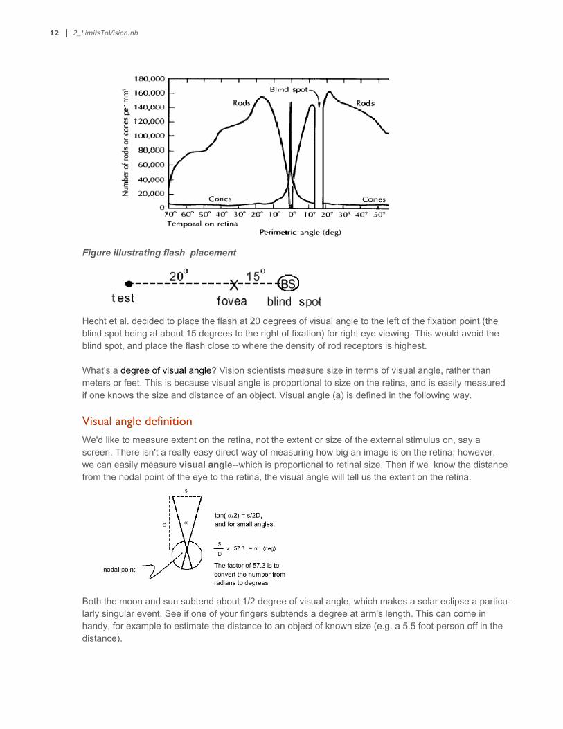
Figure illustrating flash placement

Hecht et al. decided to place the flash at 20 degrees of visual angle to the left of the fixation point (the blind spot being at about 15 degrees to the right of fixation) for right eye viewing. This would avoid the blind spot, and place the flash close to where the density of rod receptors is highest.

What's a degree of visual angle? Vision scientists measure size in terms of visual angle, rather than meters or feet. This is because visual angle is proportional to size on the retina, and is easily measured if one knows the size and distance of an object. Visual angle (a) is defined in the following way.

Visual angle definitionWe'd like to measure extent on the retina, not the extent or size of the external stimulus on, say a screen. There isn't a really easy direct way of measuring how big an image is on the retina; however, we can easily measure visual angle--which is proportional to retinal size. Then if we know the distance from the nodal point of the eye to the retina, the visual angle will tell us the extent on the retina.

Both the moon and sun subtend about 1/2 degree of visual angle, which makes a solar eclipse a particu-larly singular event. See if one of your fingers subtends a degree at arm's length. This can come in handy, for example to estimate the distance to an object of known size (e.g. a 5.5 foot person off in the distance).

Really small angles are measured in minutes (60ths of a degree), and really, really small angles in seconds (60ths of a minute). It it is difficult for us to resolve details finer than about 1 minute of arc. But there are special conditions (called hyperacuity) under which we can detect spatial displacements of 10s of seconds of arc, or even less.


Both the moon and sun subtend about 1/2 degree of visual angle, which makes a solar eclipse a particu-larly singular event. See if one of your fingers subtends a degree at arm's length. This can come in handy, for example to estimate the distance to an object of known size (e.g. a 5.5 foot person off in the distance).

Really small angles are measured in minutes (60ths of a degree), and really, really small angles in seconds (60ths of a minute). It it is difficult for us to resolve details finer than about 1 minute of arc. But there are special conditions (called hyperacuity) under which we can detect spatial displacements of 10s of seconds of arc, or even less.

Flash sizeHow large should the spot of light be?

Below is a characteristic plot of the way human light thresholds vary with the diameter of a flash (in minutes of arc, where 60 minutes = 1 degree).

Threshold vs. spot size

There is little difference in the number of quanta required for detection of spots of light of various sizes as long as their diameters are less than 10 min (1/6 deg). 1000 quanta spread over 1 min is as easily detected as 1000 quanta spread over 10 min; but 1000 quanta spread over 1000 min requires more quanta in order to be detected as well. This process of the visual system is called spatial integration.

Hecht, Schlaer, and Pirenne decided that a spot with diameter of less than 10 min would guaran-tee that detection would not be limited by the eye's inability to spatially integrate light energy. The degree of spatial integration does depend on where in the retina it is measured, state of adaptation, and duration. Hecht et al. used a size suitable for the conditions of their experiment.

Flash durationWhat should the duration of the stimulus be? Below is a characteristic plot of how human thresh-

olds vary as a function of the duration of a flash. (in this case, a 4.5 min spot at 15 deg)Analogous to spatial integration, the eye also shows temporal integration. In this case, there is

little difference in the threshold in terms of the number of quanta for a durations under 100 milliseconds. 1000 quanta is detected as easily when spread over 1 ms as when spread over 100 ms. A useful number to remember is that under scotopic conditions, the temporal integration time of the eye is about 200 msec, but is significantly shorter under photopic conditions (~100 msec). (This is one of the con-straints that go into deciding on TV and video display refresh rates.)

Hecht, Schlaer, and Pirenne played it safe and used a 1 millisecond duration for their flash.


Threshold vs. duration

Flash wavelengthWhat should the wavelength of the light be? Psychophysical measurements again provide the answer.

Sensitivity vs. wavelength

As you can see from the figure, human thresholds vary with the wavelength of light. (Note that this plot shows the log of the reciprocal of threshold--so measure of sensitivity.) Different wavelengths of light vary in the efficiency with which their photons are transduced, and thus detected. This is a direct consequence of the absorption properties of the photoreceptors. For scotopic (rod) vision, around 500 nm is optimal (Hecht used 510nm). (For photopic vision, 555nm is optimal).


As you can see from the figure, human thresholds vary with the wavelength of light. (Note that this plot shows the log of the reciprocal of threshold--so measure of sensitivity.) Different wavelengths of light vary in the efficiency with which their photons are transduced, and thus detected. This is a direct consequence of the absorption properties of the photoreceptors. For scotopic (rod) vision, around 500 nm is optimal (Hecht used 510nm). (For photopic vision, 555nm is optimal).

Summary of experimental conditions

To summarize the conditions chosen by Hecht et al.:• The subjects were dark adapted and viewed a disk of light against a dark background• The flash was placed 20 degrees to the left of the fixation mark (right eye)• The flash size was 10 minutes of arc• The duration of the flash was 1 ms.• The wavelength was 510 nanometers.Hecht et al., did not have to make the measurements necessary to determine these

conditions themselves. The data to make the decisions for their experiment were all in the existing psychophysical literature of the time. If we repeated the experiment today, we could make some minor improvements in their choices, but the results would not be substantially different.

Figure schematic: Spot placement relative to eye

(Not to scale)

Results of the experiment

Threshold measured

For the criterion of 60% yes responses, about 90 quanta (on average) were required, measured at the cornea--the entrance to the eye.

This is an amazingly small figure! But we're not done.


For the criterion of 60% yes responses, about 90 quanta (on average) were required, measured at the cornea--the entrance to the eye.

This is an amazingly small figure! But we're not done.

What is the significance of a threshold of 90 quanta?

Of the 90 quanta, measurements showed that about 3% gets reflected from the cornea. About 50% of the remaining light gets transmitted all the way through the vitreous fluid of the eye. Finally of this remaining light, a further 80% is lost between receptors or isn’t transduced by the receptors. After making these adjustments, that they concluded that only about 9 photons (on average) were actually required at the receptors to "see" a flash...

Photon losses in optic media

But there was “one more thing”...Hecht et al. went yet one further step, to draw the remarkable conclu-sion that:

One photon is sufficient to activate one rod.

Their logic was simple. If 9 photons were to be spread over about 500 rods (their estimate), the chances that 2 photons get absorbed by one rod is very small. (Current estimate of the number of rods in this part of the retina in a 10' diameter spot is closer to 350). Assuming independence of absorptions, you can try to calculate the odds of more than 2 yourself.

Fast-forward four decades: "Going inside the box"

The basic results and conclusions of this psychophysical experiment still stand today. What about the neurophysiology?A little less than 40 years after Hecht et al. published their results, Baylor et al. (1979) were able to suck single toad rods into electrodes and measure current responses to single photon events (see figure)


Rods and cones schematic

Photon "bumps" in rod current

From: Baylor, D. A., Lamb, T. D., & Yau, K. W. (1979). Responses of retinal rods to single photons. Journal of Physiology, Lond., 288, 613-634.

Preview: Computational Theory for Light DiscriminationConsider again the psychometric function. The psychometric function showed that the transition from invisible to visible was not abrupt. This basic observation is seen in almost all studies of sensory thresh-olds. So why is the psychometric function sigmoidal, rather than a step function? Variability may be due to the statistics of photon emission and absorption, human responses, and neural transmission. Signal detection theory was developed 1940’s and 1950’s to describe the ability to detect, discriminate, and estimate signals in the presence of variability or "noise", without caring much about exactly where the noise comes from, just about its properties and effects on sensory decisions.

We now generalize the light detection task to light discrimination--where the observer has to decide which of two lights is brighter.


Consider again the psychometric function. The psychometric function showed that the transition from invisible to visible was not abrupt. This basic observation is seen in almost all studies of sensory thresh-olds. So why is the psychometric function sigmoidal, rather than a step function? Variability may be due to the statistics of photon emission and absorption, human responses, and neural transmission. Signal detection theory was developed 1940’s and 1950’s to describe the ability to detect, discriminate, and estimate signals in the presence of variability or "noise", without caring much about exactly where the noise comes from, just about its properties and effects on sensory decisions.

We now generalize the light detection task to light discrimination--where the observer has to decide which of two lights is brighter.

Above, our generative model for light transmission in essence had a knob which could continuously vary the light intensity. But the observer was asked to make a discrete decision. Our theoretical develop-ment will be more straightforward if we match the signal space to the decision space. We could ask an observer to estimate the amount of light (e.g. on a scale of 1 to 100, and psychophysicists sometimes do this). But psychophysicsts usually prefer to make the signal space simple, and discrete. Let’s con-sider the discrete, in fact, binary case.

A generative model for light intensity discrimination

Schematic of set-up for ideal photon counter

Physical model for light, two switch settingsAs above, let's define a Poisson distribution with a mean represented by the variable name mean, with a function to draw a sample from this distribution. Let highmean = 7 for the "high" setting, and lowmean =5 for the "low" setting. So at a given time, mean can take on only one of two values: mean = high-mean or lowmean.

In[15]:= numberofphotons[mean_] := RandomInteger[PoissonDistribution[mean]];dotsize = 0.01;highmean = 7;lowmean = 4;

▶ 3. Test the code above. Simulate turning the switch to “high”, draw a few samples, and then to “low” and draw some samples. What would happen if you used = instead of := in the above function definition?

We'll define a "blank" graphics display that we'll use to "turn off" the display--i.e. make it black.


In[19]:= blank = Graphics[{PointSize[dotsize], Black, Point /@ {{}, {}}},AspectRatio → 1, Frame → False, FrameTicks → None,Background → GrayLevel[0.0], PlotRange → {{-0.2, 1.2}, {-0.2, 1.2}}];

flash =

blank;

We could keep the display within this notebook, but let's create a new one and insert the graphics object "flash" in it, and at the same time declare it as a Dynamic variable. We do this so that it will automati-cally change whenever we do something to the flash variable in our home notebook.

In[21]:= CreateDocument[Dynamic[flash], ShowCellBracket → False, WindowSize → {300, 300},WindowElements → {}, Background → Black, NotebookFileName → "Flash Display"];

Now we'll create a function called "twoflashes" that we can call whenever we want to display a pair of flashes in our "Flash Display" window. We use RandomInteger[1] to simulate a "coin flip" to decide whether the switch (our "state of the world" or signal) is set to high or low.

In[22]:= twoflashes := Module[{tempmean},If[RandomInteger[1] ⩵ 1, firstmean = lowmean;secondmean = highmean, firstmean = highmean;secondmean = lowmean];

numhighsample = numberofphotons[firstmean];highsample = Table[RandomReal[{0, 1}, 2], {numhighsample}];(*pick a random 2D location for the dot*)flash = Graphics[{PointSize[dotsize], Red, Point /@ highsample},

AspectRatio → 1, Frame → False, FrameTicks → None,Background → GrayLevel[0.0], PlotRange → {{-0.2, 1.2}, {-0.2, 1.2}}];

Pause[1]; flash = blank; Pause[.5];numhighsample = numberofphotons[secondmean];highsample = Table[RandomReal[{0, 1}, 2], {numhighsample}];flash = Graphics[{PointSize[dotsize], Red, Point /@ highsample},

AspectRatio → 1, Frame → False, FrameTicks → None,Background → GrayLevel[0.0], PlotRange → {{-0.2, 1.2}, {-0.2, 1.2}}];

Pause[1];

flash = blank;]

Whenever you evaluate the following cell, it should present a pair of "flashes" in the "Flash Display" notebook.

In[31]:= twoflashes

Now you be the "sensor" that counts dots (aka “photons”)--and with each flash, decide whether it was the first or the second flash that was caused by the high switch setting.

What do think is the best strategy--i.e. one that enables you to get the highest proportion of correct guesses?

This is an example of a two-alternative forced-choice experiment (2AFC). More on this later.


Now you be the "sensor" that counts dots (aka “photons”)--and with each flash, decide whether it was the first or the second flash that was caused by the high switch setting.

What do think is the best strategy--i.e. one that enables you to get the highest proportion of correct guesses?

This is an example of a two-alternative forced-choice experiment (2AFC). More on this later.

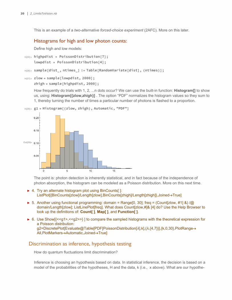
Histograms for high and low photon counts: Define high and low models:

In[24]:= highpdist = PoissonDistribution[7];lowpdist = PoissonDistribution[4];

In[26]:= sample[dist_, ntimes_] := Table[RandomVariate[dist], {ntimes}];

In[27]:= zlow = sample[lowpdist, 2000];zhigh = sample[highpdist, 2000];

How frequently do trials with 1, 2, ...n dots occur? We can use the built-in function: Histogram[] to show us, using: Histogram[{zlow,zhigh}] . The option “PDF” normalizes the histogram values so they sum to 1, thereby turning the number of times a particular number of photons is flashed to a proportion.

In[29]:= g1 = Histogram[{zlow, zhigh}, Automatic, "PDF"]

Out[29]=

The point is: photon detection is inherently statistical, and in fact because of the independence of photon absorption, the histogram can be modeled as a Poisson distribution. More on this next time.

▶ 4. Try an alternate histogram plot using BinCounts[ ]: ListPlot[{BinCounts[zlow]/Length[zlow],BinCounts[zhigh]/Length[zhigh]},Joined→True]

▶ 5. Another using functional programming: domain = Range[0, 30]; freq = (Count[zlow, #1] &) /@ domain/Length[zlow]; ListLinePlot[freq]. What does Count[zlow,#]& [4] do? Use the Help Browser to look up the definitions of: Count[ ], Map[ ], and Function[ ].

▶ 6. Use Show[{<<g1>,<<g2>>} ] to compare the sampled histograms with the theoretical expression for a Poisson distribution: g2=DiscretePlot[Evaluate@Table[PDF[PoissonDistribution[λ],k],{λ,{4,7}}],{k,0,30},PlotRange→All,PlotMarkers→Automatic,Joined→True]

Discrimination as inference, hypothesis testing

How do quantum fluctuations limit discrimination?

Inference is choosing an hypothesis based on data. In statistical inference, the decision is based on a model of the probabilities of the hypotheses, H and the data, k (i.e., x above). What are our hypothe-ses?

Think of the task in terms of signal transmission. The “sender” wishes to set the light switch to one of two positions, corresponding to a high and low average light intensities. The signal (or hypothesis space) is simple, the states of the switches: H = SL (low), or H = SH (high). The idea is that we have two hypotheses that each determine a conditional probability distribution.


How do quantum fluctuations limit discrimination?

Inference is choosing an hypothesis based on data. In statistical inference, the decision is based on a model of the probabilities of the hypotheses, H and the data, k (i.e., x above). What are our hypothe-ses?

Think of the task in terms of signal transmission. The “sender” wishes to set the light switch to one of two positions, corresponding to a high and low average light intensities. The signal (or hypothesis space) is simple, the states of the switches: H = SL (low), or H = SH (high). The idea is that we have two hypotheses that each determine a conditional probability distribution.

Thus, given a measurement of x photons, there is an inherent ambiguity in determining the cause or signal--SL or SH? Next time, we will develop signal detection theory, and then see how to extend the fundamental principles of SDT to general perceptual inference for image patterns and a range of visual tasks. We effectively turn the generative problem on its head, and derive the best guesser for deciding light switch position based on a measure of light intensity.

From the starting point of signal detection theory, we’ll develop the theory of ideal observers, and then later, a computational framework to understand perception generally as a process of statistical inference.

ReferencesAzevedo A, Rieke F. Experimental conditions alter phototransduction: the implications for retinal process-ing at visual threshold. Journal of Neuroscience 31(10):3670-3682. 2011Barlow, H. B. (1962). A method of determining the overall quantum efficiency of visual discriminations. Journal of Physiology (London), 160, 155-168.Barlow, H. B., & Mollon, J. D. (1982). The Senses. Cambridge: Cambridge University Press.Baylor, D. A., Lamb, T. D., & Yau, K. W. (1979). Responses of retinal rods to single photons. Journal of Physiology, Lond., 288, 613-634.Cornsweet, T. N. (1970). Visual Perception . New York: Academic Press.Green, D. M., & Swets, J. A. (1974). Signal Detection Theory and Psychophysics . Huntington, New York: Robert E. Krieger Publishing Company.Hecht, S., Shlaer, S., & Pirenne, M. H. (1942). Energy, quanta, and vision. Journal of General Physiol-ogy, 25, 819-840.Rieke F, Rudd ME. The challenges natural images pose for visual adaptation. Neuron 64:605-616, 2009Rose, A. (1948). The sensitivity performance of the human eye on an absolute scale. Journal of the Optical Society of America, 38, 196-208.Pelli, D. G. (1990). The quantum efficiency of vision. In C. Blakemore (Ed.), Vision:Coding and Effi-ciency Cambridge: Cambridge University Press.

© 2008, 2010, 2103, 2015, 2017 Daniel Kersten, Computational Vision Lab, Department of Psychology, University of Minnesota.courses.kersten.org


computational vision u. minn. psy 5036 daniel kersten lecture 2: limits...

Documents