Computer Aided Thermal Computer Aided Thermal Fluid AnalysisFluid Analysis

Lecture 7Lecture 7

Dr. Ming-Jyh ChernDr. Ming-Jyh Chern

ME NTUSTME NTUST

Road Map for TodayRoad Map for Today

• Example of arbitrary coupleExample of arbitrary couple

• Solver for a steady laminar flow Solver for a steady laminar flow problemproblem

• Setup solver step by stepSetup solver step by step

• Simple post-processing – Simple post-processing – velocity and contour plotsvelocity and contour plots

• User Guide Chapter 8User Guide Chapter 8

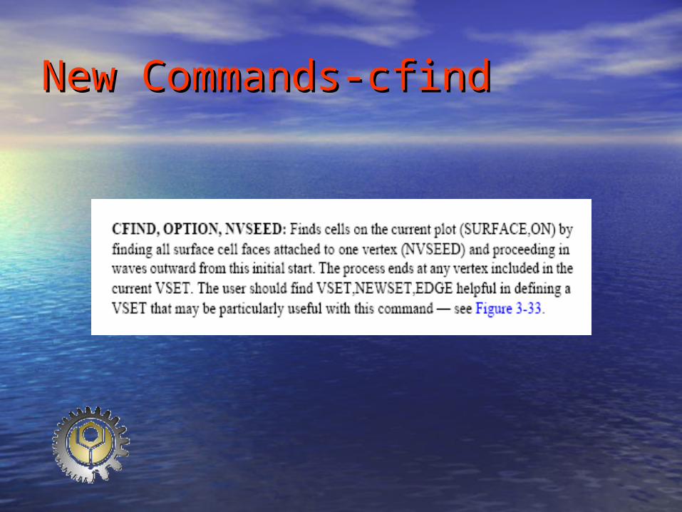
New Commands-cfindNew Commands-cfind

New Commands-cfindNew Commands-cfind

New Commands-cfindNew Commands-cfind

New Commands-vproNew Commands-vpro

New Commands-vproNew Commands-vpro

New Commands-vproNew Commands-vpro

New Commands-crefineNew Commands-crefine

New Commands-crefineNew Commands-crefine

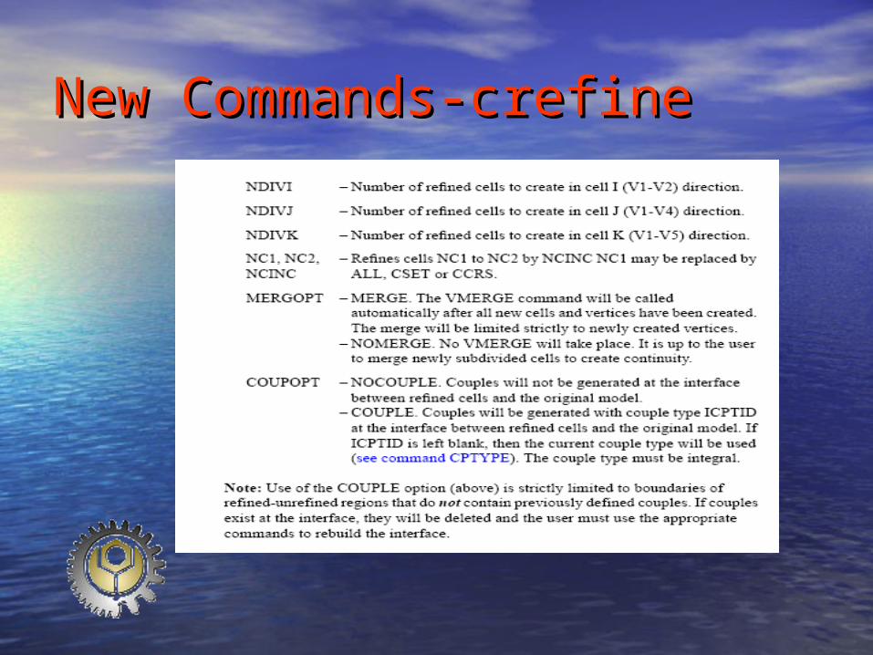
New Commands-crefineNew Commands-crefine

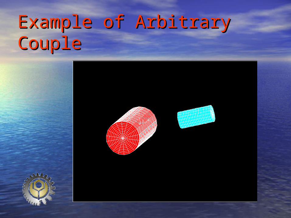
Example of Arbitrary CoupleExample of Arbitrary Couple

Example of Arbitrary CoupleExample of Arbitrary Couple

Example of Arbitrary CoupleExample of Arbitrary Couple

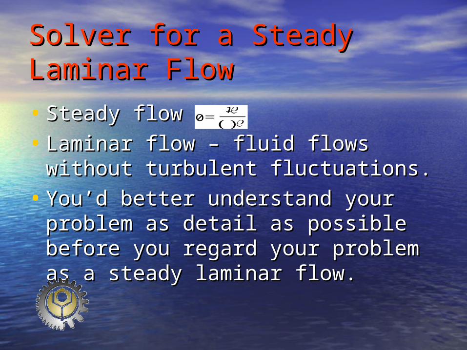
Solver for a Steady Laminar Solver for a Steady Laminar FlowFlow

• Steady flow – Steady flow –

• Laminar flow – fluid flows without Laminar flow – fluid flows without turbulent fluctuations.turbulent fluctuations.

• You’d better understand your You’d better understand your problem as detail as possible before problem as detail as possible before you regard your problem as a steady you regard your problem as a steady laminar flow.laminar flow.

0

t

Before you go to the solverBefore you go to the solver

• You need to finished tasks of pre-You need to finished tasks of pre-processing:processing:– Mesh setup upMesh setup up– Fluid property and thermofluid model Fluid property and thermofluid model

specificationspecification– Definition of boundary type and location Definition of boundary type and location

Quickest Way to Solve Quickest Way to Solve Steady Flow ISteady Flow I

• Step 1 – Select Step 1 – Select Steady StateSteady State from the from the TiTime domainme domain pop-up menu in the STAR-G pop-up menu in the STAR-GUIdeUIde

• Step 2 – Go to the Solution Controls foldStep 2 – Go to the Solution Controls folder and open the Solution Method panel. er and open the Solution Method panel. Choose Choose Steady StateSteady State or or Pseudo-TransiPseudo-Transientent

Quickest Way to Solve Quickest Way to Solve Steady Flow IISteady Flow II

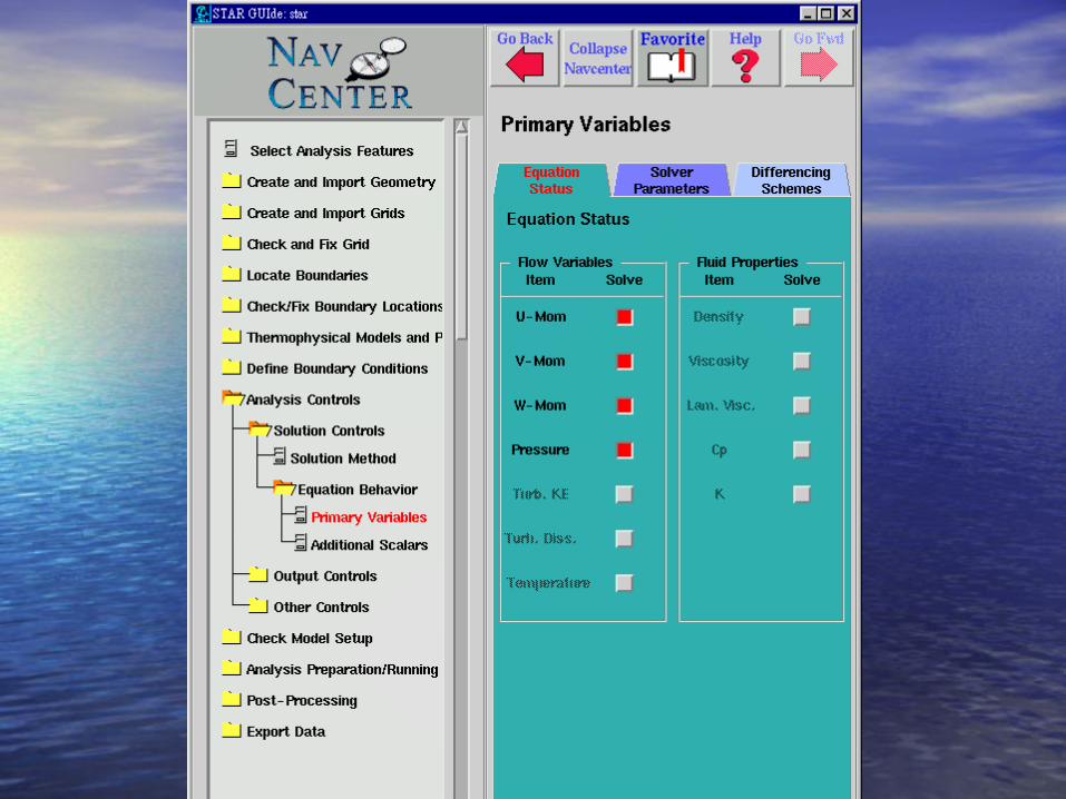
• Step 3 – In the Primary Variables Step 3 – In the Primary Variables panel, panel,

• Step 4 – Relaxation and Solve Step 4 – Relaxation and Solve Parameters, set up tolerance and Parameters, set up tolerance and iterative numberiterative number

• Step 5 - Choose one of the available Step 5 - Choose one of the available Differential Schemes. Differential Schemes.

Quickest Way to Solve Quickest Way to Solve Steady Flow IIISteady Flow III

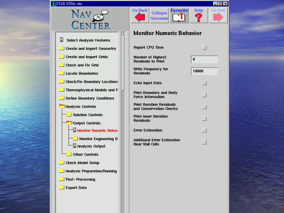
• Step 6 – Output control. Monitor Step 6 – Output control. Monitor Numeric BehaviorNumeric Behavior

• Step 7 – Output control. Analysis Step 7 – Output control. Analysis controlcontrol

• Step 8 - Save & Check model setup.Step 8 - Save & Check model setup.

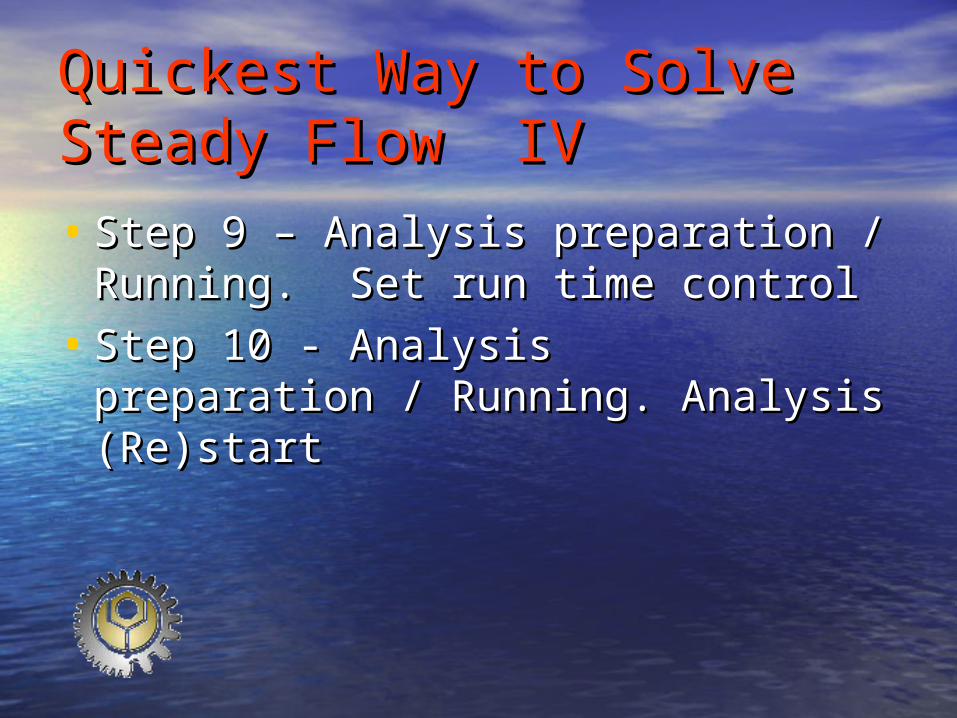
Quickest Way to Solve Quickest Way to Solve Steady Flow IVSteady Flow IV

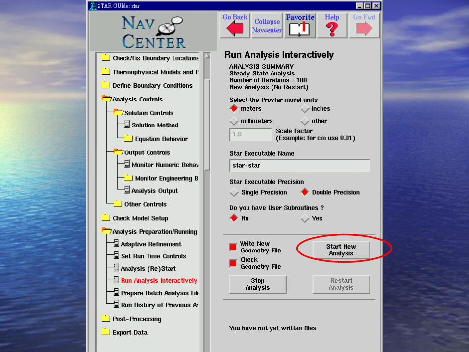
• Step 9 – Analysis preparation / Step 9 – Analysis preparation / Running. Set run time controlRunning. Set run time control

• Step 10 - Analysis preparation / Step 10 - Analysis preparation / Running. Analysis (Re)startRunning. Analysis (Re)start

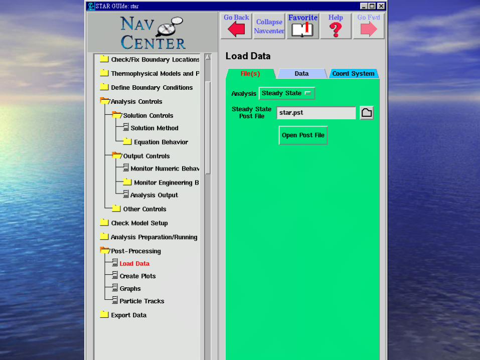
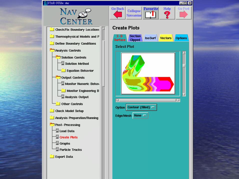
PostProcessingPostProcessing

• Load DataLoad Data

• Create plotsCreate plots

• Export dataExport data

Homework 4Homework 4

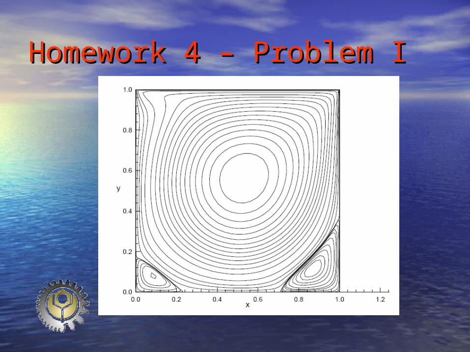
• Simulate a 2-D lid-driven cavity flow at Re = 100 and 1,000. PleasSimulate a 2-D lid-driven cavity flow at Re = 100 and 1,000. Please compare your velocity results with Ghia e compare your velocity results with Ghia et alet al.’s(1982) data alo.’s(1982) data along the vertical central line. ng the vertical central line.

• Simulate a 2-D uniform flow past a circular cylinder at Re = 40. PrSimulate a 2-D uniform flow past a circular cylinder at Re = 40. Predict the length edict the length ll of the wake behind the circular cylinder of diam of the wake behind the circular cylinder of diameter eter dd. .

• Choose one of them. Give velocity and pressure contour plot firsChoose one of them. Give velocity and pressure contour plot first. Subsequently, you have to make the required comparison.t. Subsequently, you have to make the required comparison.

• Due date: 15 May, 2006Due date: 15 May, 2006• Ghia, U., Ghia, K.N., and Shin, C.T. 1982 High-Re solutions for incoGhia, U., Ghia, K.N., and Shin, C.T. 1982 High-Re solutions for inco

mpressible flow using the Navier-Stokes equations and a multigrmpressible flow using the Navier-Stokes equations and a multigrid method. id method. Journal of Computational PhysicsJournal of Computational Physics 4848, 387-411., 387-411.

Homework 4 – Problem IHomework 4 – Problem IU

L

0.5L

Re = UL/

Compare your solution of horizontal velocity component with Ku et al.’s along this central vertical line.

Homework 4 – Problem IHomework 4 – Problem IReRe

yy 100100 1,0001,000

1.0001.000 1.01.0 1.01.0

0.97660.9766 0.841230.84123 0.659280.65928

0.96880.9688 0.788710.78871 0.574920.57492

0.96090.9609 0.737220.73722 0.511170.51117

0.95310.9531 0.687170.68717 0.466040.46604

0.85160.8516 0.231510.23151 0.333040.33304

0.73440.7344 0.003320.00332 0.187190.18719

0.61720.6172 -0.13641-0.13641 0.057020.05702

0.50.5 -0.20581-0.20581 -0.06080-0.06080

0.45310.4531 -0.21090-0.21090 -0.10648-0.10648

0.28130.2813 -0.15662-0.15662 -0.27805-0.27805

0.17190.1719 -0.10150-0.10150 -0.38289-0.38289

0.10160.1016 -0.06434-0.06434 -0.2973-0.2973

0.07030.0703 -0.04775-0.04775 -0.2222-0.2222

0.06250.0625 -0.04192-0.04192 -0.20196-0.20196

0.05470.0547 -0.03717-0.03717 -0.18109-0.18109

0.00.0 00 00

Profile of velocity component u along the central vertical line.

Homework 4 – Problem IHomework 4 – Problem I

Homework 4 – Problem IHomework 4 – Problem I

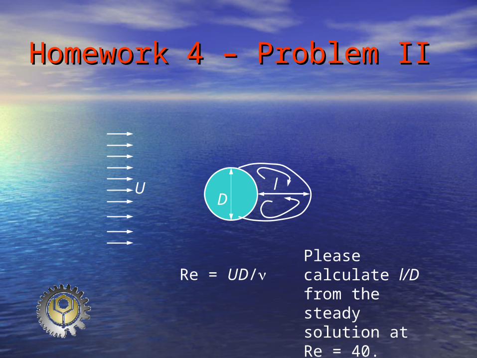
Homework 4 – Problem IIHomework 4 – Problem II

UD

Re = UD/

l

Please calculate l/D from the steady solution at Re = 40.

Homework 4 – Problem IIHomework 4 – Problem II

Homework 4 – Problem IIHomework 4 – Problem II

Homework 4 – Problem IIHomework 4 – Problem II