Computer Animation 7-Physics

SS 18

Prof. Dr. Charles A. Wüthrich,

Fakultät Medien, Medieninformatik

Bauhaus-Universität Weimar

caw AT medien.uni-weimar.de

Introduction

• While animating through kynematics may be interesting for plenty of applications, integrating physics is more difficult and a challenging problem

• The easiest way of integrating physics is rigid body simulation• While physics is concerned with the exactness of the

representation, animation is more interested in „credible“ effects, and in rendering frame by frame

• Having to deal with the system at discrete time samples creates numerical problems in the solution methods which are not simple to deal with

Recap on physics (physics 101)

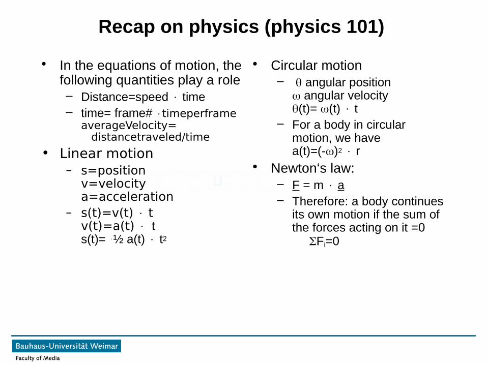
• In the equations of motion, the following quantities play a role– Distance=speed time– time= frame# timeperframe

averageVelocity= distancetraveled/time

• Linear motion– s=position

v=velocitya=acceleration

– s(t)=v(t) tv(t)=a(t) ts(t)= ½ a(t) t2

• Circular motion– angular position

angular velocity(t)= (t) t

– For a body in circular motion, we have a(t)=(-)2 r

• Newton‘s law:– F = m a– Therefore: a body continues

its own motion if the sum of the forces acting on it =0 Fi=0

Recap on physics (physics 101)

• Remember the definition of center of mass

– The point at which the object is balanced in all directions

– If an external force is applied to a body in line with its center of mass, then the body would move as if it was a point at the center of mass C

• Torque is the tendency of a force to produce circular motion

– It is produced by a force off center to the center of mass

– = r F– Clearly, F and r

• An object does not move if Fi=0 and i=0

C F

CF

r

Recap on physics (physics 101)

• Linear springs:– Hooke‘s law:

F= -k x, where x is the change from the equilibrium length of the spring

• Friction:– Static:

Fs = s fN

where Fs = frictional forces=static friction coefficientfN = normal force

– Kinetic: Fk = k fN

with similar coefficient definitions as in static friction

• Momentum: m v– In a closed system, total

momentum does not vary• Angular momentum:

L=rpwhere r=vector from center of rotationp=momentum (m v)

– Note that = dL/dt

– In a closed system, total angular momentum does not vary

• Inertia tensor: the resistence of an object to change its angular momentum

Rigid body simulation

• If one wants to simulate rigid bodies, many forces act on them

• Such forces vary in time conti-nuously and in a non linear way

• Therefore it is not enough to evaluate velocities and acce-lerations at fixed timesteps t

• Evaluating the velocities at t0, t0+t, t0+2t does not generate a correct movement, and slowly drifts away from the correct solution

• This solution method is an example of the Euler integration method

• The accuracy of the method is determined by the size of the time step

• Obviously the shorter the time step, the more computations are needed

• A better way of integrating the equations bases on the Runge Kutta method

– In particular, often 2nd order Runge Kutta (midpoint method) is used

– Remember, the order of the RK method is the magnitude of the error term

– Even higher order ones, 4th or 5th ones are used

Motion equations for a rigid body

• To develop the equation of motion for a rigid body, we have to apply some of the physics presented before

• When a force is applied to a rigid body, the force and the relative torque are applied to the body

• To uniquely solve for the resulting motions of interacting bodies, linear and angular momentum have to be conserved

• Finally, to calculate the angular momentum the distribution of an object mass in space has to be characterized with its inertia tensor.

Orientation and rotational movement

• Similar to position, velocity and acceleration, 3D objects have

– orientation, – angular velocity and – angular acceleration

which vary in time• Let R(t) represent the object

rotation• Angular velocity (t) is the rate

at which the object is rotated (independent from linear velocity)

• The direction of (t) indicates the orientation of the axis about which the object is rotating

• The magnitude of (t) gives the speed of rotation in revs per unit time

Orientation and rotational movement

• Consider a point a whose position is defined in space relative to a point b=x(t).

• Let a‘s position be defined by r(t)

• Suppose that a is rotating and the axis passes through b

• The change in r(t) is the cross product of r(t) and (t) r (t)=(t) r(t) |r (t)|=|(t)| |r(t)| sin

• Now consider an object that has a distribution of mass in space

• Its orientation can be seen as a transformed version of the object local coord. system

• Its columns can be seen as vectors defining the relative positions of the object points

• Thus, the change of the rotation matrix can be computed by taking the cross product of (t) with each of the columns of R(t) R(t)=[R1(t) R2(t) R3(t)] R (t)= [(t)R1(t) (t)R2(t) (t) R3(t)]

r(t)

a=b+r(t)(t)

b=x(t)

Orientation and rotational movement

• By defining a special matrix to represent cross products:

• It follows R(t)= (t)* R(t)

• Consider now a point Q on a rigid object

• Its position in local coord system does not change

• Its pos in world coords is q(t)=R(t)q+x(t)

• Differentiating this one obtains the velocity

• The change in orientation is given by the eq on the left

• Combining these, one obtains q(t)=(t)* r(t)q+v(t)

• Substituting one obtains q(t)=(t)(q(t)-x(t))+v(t)

A×B=[A y⋅B z−A z⋅B y

−(A z⋅Bx )+Ax⋅B zA x⋅B y−A y⋅Bx ]=

=[0 −A z A yAz 0 −A x

−A y Ax 0 ][BxB yB z ]=A

¿B

Center of mass

• The center of mass of a body is defined as the integral of the differential mass times its position in the object

• In a body with discrete masses, then the center of mass is at qi(t), the center of mass is at x(t)=miqi(t)/mi

Forces and torque

• A linear force applied to a mass gives rise to a linear acceleration F=ma (Newton‘s law)

• The various forces applied to a point sum up F(t)=fi(t)

• The torque arising from the application of forces acting on a point of an object is given by i(t)=(q(t)-x(t)) fi(t) (t)=i(t)

Momentum

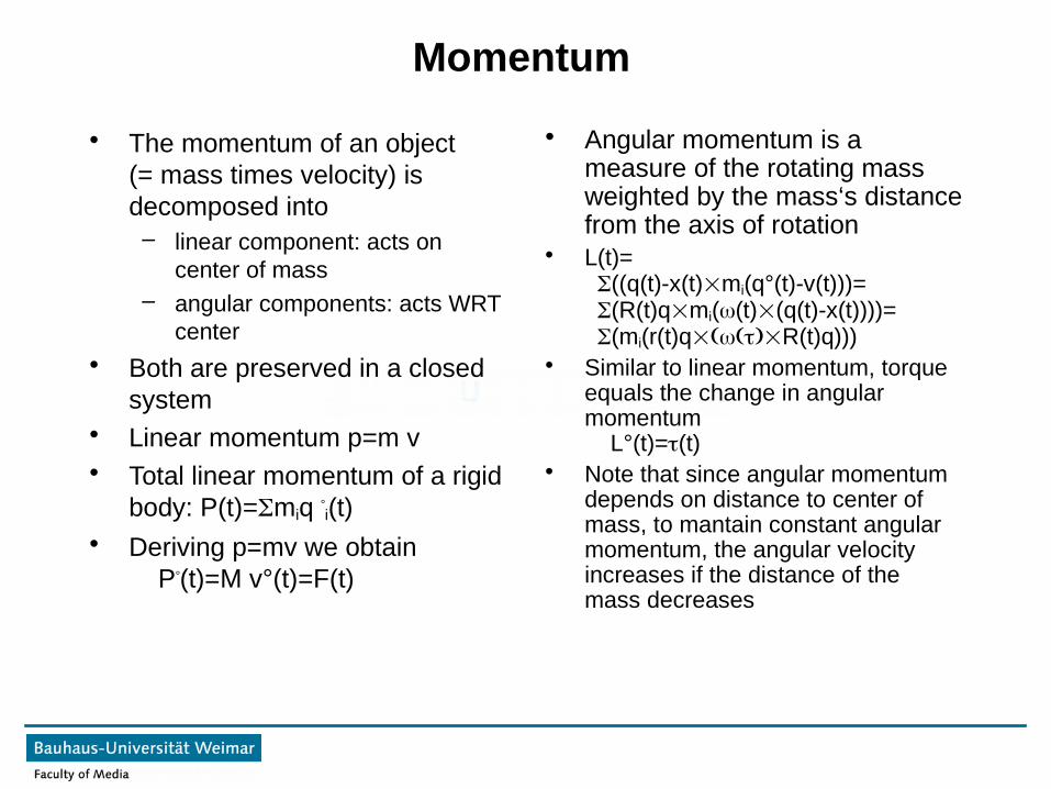
• The momentum of an object (= mass times velocity) is decomposed into

– linear component: acts on center of mass

– angular components: acts WRT center

• Both are preserved in a closed system

• Linear momentum p=m v• Total linear momentum of a rigid

body: P(t)=miq i(t)• Deriving p=mv we obtain

P(t)=M v°(t)=F(t)

• Angular momentum is a measure of the rotating mass weighted by the mass‘s distance from the axis of rotation

• L(t)= ((q(t)-x(t)mi(q°(t)-v(t)))= (R(t)qmi((t)(q(t)-x(t))))= (mi(r(t)qR(t)q)))

• Similar to linear momentum, torque equals the change in angular momentum L°(t)=(t)

• Note that since angular momentum depends on distance to center of mass, to mantain constant angular momentum, the angular velocity increases if the distance of the mass decreases

Inertia tensor

• Angular momentum is related to angular velocity the same way linear momentum is related to linear velocity P(t)=M v(t)

• We have L(t)=I(t)(t)

• The distrib. of mass of the obj. in space is defined through a matrix, the inertia tensor I(t)

where the matrix terms are computed by integrating over the object, and I is symmetric

• In general,Ixx=∫∫∫(q)(qy2+qz2)dxdydzwhere is the density of at an obj. point q=(qx,qy,qz)

• In the case of discrete masses Ixx=mi(yi2+zi2), Ixy=mixiyi

Iyy=mi(xi2+zi2), Ixz=mixizi Izz=mi(xi2+yi2), Iyz=miyizi

• In a center of mass centered obj space, the intertia tensor of a transformed object depends on the obj orientation but not on its position, and therefore it depends on time

• It can be transformed with I(t)=R(t)IobjR(t)T

I obj=[I xx I xy I xzI yx I yy I yzI zx I zy I zz ]

Motion equations

• The state of an object can be determined by the vector containing

– Position– Orientation– Linear momentum– Angular momentum

• Object mass and its object space inertia tensor Iobj do not change in time

• At any time, the following quantities can be computed:

Inertia tensor I(t)=R(t)IobjR(t)T Angular vel. (t)=I(t)-1L(t) Linear vel. v(t)=P(t)/M

• Now the time derivative can be formed:

This is enough to run a simulation

• A differential equation solver can now be used

S ( t )=[x ( t )R ( t )P ( t )L( t )

] ddt S ( t )=

ddt [

x ( t )R( t )P( t )L ( t )

]=[v ( t )

ω ( t )¿R ( t )F ( t )τ ( t )

]

• As the simplest solver, one can use Euler‘s method– The values of the state array are updated by multiplying their time

derivatives by the length of the time step

• In practice, Runge-Kutta methods are used, especially 4th order ones• Particular care has to be taken in updating the orientation of an object,

because if the derivative info is used to update the orientation matrix, then the columns of the matrix can become nonorthogonal and not of unit length

• Here it is wise to renormalize after each step• Alternatively, one can update

– by applying the axis-angle rotation generated by angular velocity– By using quaternions

Motion equations

t0+t

t0

t0+2t

Ordinary differential equations

• Problem involving ordinary differential equations (ODE) can be reduced to the study of first order differential equations

• For example, the problem d2y/dx2+q(x)dy/dx=r(x)

can be rewritten as the two first order equations

dy/dx=z(x) dz/dx=r(x)-q(x)z(x)

• The generic problem in ordinary differential equations can be thus reduced to the study of a set of N first order differential equation for the functions yi (i=1,2,...,N) dyi(x)/dx=f´i(x,y1,...yN)where the fi are known

• A problem involving ODEs is not determined completely by its equations.

• The boundary conditions also determine how to solve the problem.

• Boundary conditions are algebraic conditions on the values of the functions yi

• In general, they can be satisfied at the discrete specified points, but do not hold inbetween these points

• They can be as simple as requiring to pass through a certain point, or as complicated as a complex algebraic expression

Ordinary differential equations

• Boundary conditions divide into two categories:

– Initial value problems: here all yi are given at some starting value xs, and one wants to find the yi at some end point xf, or at some discrete list of points

– Two-point boundary value problems: here some conditions are set at xs, and some at xf

• We will deal only with the first class

• The main idea of a method for initial value is the following:

– Rewrite dx and dy as finite y and x and multiply the equations by x

• This gives formulas for the change in the functions when the variable x is stepped at stepsize x

• For x small, one obtains a decent approximation of the diff. Equation

• Literal implementation of this method is called Euler‘s method

– Euler method is not accurate compared to other methods using the same step size

– It is not very stable either

ODE: Runge Kutta

• One way or another, all methods do the following:

– Add small increments to the functions corresponding to the derivatives multiplied by stepsizes

• Runge Kutta methods propagate a solution over an interval by combining the information from several Euler-style steps (each involving one evaluation of the f´) and then using the info obtained to match a taylor series up to some higher order

• The formula for the Euler method is yn+1=yn+hf´(xn,yn)where h is the step chosen (i.e. xn+1=xn+h)

• The problem with this is that info on the derivative change goes lost, since only info at the start of the interval (at xn) is used

• This means that the step‘s error is only one power of h smaller than the correction, thus yn+1=yn+hf´(xn,yn)+O(h2)

• By definition, we call a method such that its error term is O(hn+1) as method of order n

x3x1 x2

ODE: Runge Kutta

• Suppose to use a step like before (yn+1=yn+hf´(xn,yn)) to take a „trial“ step to the midpoint of the interval

• Then use the value of both x and y at the midpoint to compute the „real“ step across the whole interval k1=hf´(xn,yn) k2=hf´(xn+½h,yn+½k1)then one can write yn+1=yn+k2+O(h3)

• Note how all of the sudden the error becomes of 3rd degree and therefore the method becomes of second order

• This by the way is second order Runge-Kutta (midpoint methd)

• In R-K the derivative at the midpoint is evaluated and used for the whole interval

x

y(x)

1

23

x

y(x)

x3x1 x2

1

23 4

5

Eul

er M

etho

dM

idpo

int M

etho

d

ODE: Runge Kutta

• Why does this work better? – Because by evaluating at the

midpoint one takes an „average“ of the derivative on the interval

– This cancels the second order error

• Of course, one can decide now to push this elimination further

• Fourth order R-K evaluates the derivative four times:

– Initial point, twice at trial midpoints, and once at the trial endpoint

– From these derivatives the final function value is computed

• k1=hf´(xn,yn) k2=hf´(xn+h/2,yn+k1/2) k3=hf´(xn+h/2,yn+k2/2) k4=hf´(xn+h,yn+k3)and the error term becomes yn+1=yn+k1/6+k2/3+k3/3 +k4/6+O(h5)

x

y(x)yn

12

3 44t

h or

der

Met

hod

yn+1

Charles A. Wüthrich

+++ Ende - The end - Finis - Fin - Fine +++ Ende - The end - Finis - Fin - Fine +++

End

Cop

yrig

ht (

c) 1

988

ILM