1

COMPUTER BASED

NUMERICAL & STATISTICAL

TECHNIQUES

MCA 106

SELF LEARNING MATERIAL

DIRECTORATE

OF DISTANCE EDUCATION

SWAMI VIVEKANAND SUBHARTI UNIVERSITY

MEERUT – 250 005,

UTTAR PRADESH (INDIA)

2

SLM Module Developed By :

Author:

Reviewed by :

Assessed by:

Study Material Assessment Committee, as per the SVSU ordinance No. VI (2)

Copyright © Gayatri Sales

DISCLAIMER

No part of this publication which is material protected by this copyright notice may be

reproduced or transmitted or utilized or stored in any form or by any means now known or

hereinafter invented, electronic, digital or mechanical, including photocopying, scanning,

recording or by any information storage or retrieval system, without prior permission from the

publisher.

Information contained in this book has been published by Directorate of Distance Education and

has been obtained by its authors from sources be lived to be reliable and are correct to the best

of their knowledge. However, the publisher and its author shall in no event be liable for any

errors, omissions or damages arising out of use of this information and specially disclaim and

implied warranties or merchantability or fitness for any particular use.

Published by: Gayatri Sales

Typeset at: Micron Computers Printed at: Gayatri Sales, Meerut.

3

COMPUTER BASED NUMERICAL & STATISTICAL TECHNIQUES (MCA – 106)

Unit-I

Floating point Arithmetic: Representation of floating point numbers, Operations,

Normalization, Pitfalls of floating point representation, Errors in numerical

computation

UNIT-II Iterative Methods: Zeros of a single transcendental equation and zeros of

polynomial using Bisection Method, Iteration Method, Regula-Falsi method, Newton

Raphson method, Secant method, Rate of convergence of iterative methods.

Unit-III

Simultaneous Linear Equations: Solutions of system of Linear equations, Gauss

Elimination direct method and pivoting, Ill Conditioned system of equations,

Refinement of solution. Gauss Seidal iterative method, Rate of Convergence

UNIT-IV Interpolation and approximation: Finite Differences, Difference tables Polynomial

Interpolation: Newton‘s forward and backward formula, Central Difference Formulae:

Gauss forward and backward formula, Stirling‘s, Bessel‘s, Everett‘s formula.

Interpolation with unequal intervals: Langrange‘s Interpolation, Newton Divided

difference formula, Hermite‘s Interpolation Approximation of function by Taylor‘s

series and Chebyshev polynomial

Unit-V

Numerical Differentiation and Integration: Introduction, Numerical Differentiation,

Numerical Integration, Trapezoidal rule, Simpson‘s rules, Boole‘s Rule, Weddle‘s

Rule Euler- Maclaurin Formula

Solution of differential equations: Picard‘s Method, Euler‘s Method, Taylor‘s

Method, Runge-Kutta methods, Predictor-corrector method, Automatic error

monitoring, stability of solution.

4

UNIT-I

Floating point Arithmetic

Representation of floating point numbers

1. To convert the floating point into decimal, we have 3 elements in a 32-bit floating point representation: i) Sign ii) Exponent iii) Mantissa

Sign bit is the first bit of the binary representation. ‗1‘ implies negative number and ‗0‘ implies positive number. Example: 11000001110100000000000000000000 This is negative number.

Exponent is decided by the next 8 bits of binary representation. 127 is the unique number for 32 bit floating point representation. It is known as bias. It is determined by 2k-1 -1 where ‗k‘ is the number of bits in exponent field. There are 3 exponent bits in 8-bit representation and 8 exponent bits in 32-bit representation.

Thus

bias = 3 for 8 bit conversion (23-1 -1 = 4-1 = 3) bias = 127 for 32 bit conversion. (28-1 -1 = 128-1 = 127) Example: 01000001110100000000000000000000 10000011 = (131)10 131-127 = 4 Hence the exponent of 2 will be 4 i.e. 24 = 16.

Mantissa is calculated from the remaining 23 bits of the binary representation. It consists of ‗1‘ and a fractional part which is determined by: Example: 01000001110100000000000000000000

The fractional part of mantissa is given by:

1*(1/2) + 0*(1/4) + 1*(1/8) + 0*(1/16) +……… = 0.625

Thus the mantissa will be 1 + 0.625 = 1.625

The decimal number hence given as: Sign*Exponent*Mantissa = (-1)0*(16)*(1.625) = 26

5

2. To convert the decimal into floating point, we have 3 elements in a 32-bit floating point representation: i) Sign (MSB) ii) Exponent (8 bits after MSB) iii) Mantissa (Remaining 23 bits) Sign bit is the first bit of the binary representation. ‗1‘ implies negative number

and ‗0‘ implies positive number. Example: To convert -17 into 32-bit floating point representation Sign bit = 1

Exponent is decided by the nearest smaller or equal to 2n number. For 17, 16 is the nearest 2n. Hence the exponent of 2 will be 4 since 24 = 16. 127 is the unique number for 32 bit floating point representation. It is known as bias. It is determined by 2k-1 -1 where ‗k‘ is the number of bits in exponent field. Thus bias = 127 for 32 bit. (28-1 -1 = 128-1 = 127) Now, 127 + 4 = 131 i.e. 10000011 in binary representation.

Mantissa: 17 in binary = 10001. Move the binary point so that there is only one bit from the left. Adjust the exponent of 2 so that the value does not change. This is normalizing the number. 1.0001 x 24. Now, consider the fractional part and represented as 23 bits by adding zeros. 00010000000000000000000

Operations

An operation, in mathematics and computer science, is an action that is carried out

to accomplish a given task. There are five basic types of computer operations:

Inputting, processing, outputting, storing, and controlling.

Although even basic computers are capable of sophisticated

processing, processors themselves are only capable of performing simple

mathematical operations. CPUs perform very complex tasks by executing billions of

individual operations per second.

When we think of computer operations, we‘re usually thinking of those involved in

processing. The arithmetic-logic unit (ALU) in the processor performs arithmetic and

logic operations on the operands according to instructions that specify each step that

must be taken to make the software do something.

6

The arithmetic operations are addition, subtraction, multiplication, and

division. There are sixteen possible logic (or symbolic) operators used to perform

tasks such as comparing two operands and detecting where bits don‘t

match. Boolean operators, which work with true/false values, include AND, OR, NOT

(or AND NOT) and NEAR. Relational operators, used for comparisons, include the

equal sign (=), the less-than symbol (<) and the greater-than symbol (>).

The ALU usually has direct input and output access to the processor controller, main

memory RAM and input/output devices. Inputs and outputs flow through the

system bus. The input consists of an instruction word that contains an operation

code, one or more operands and sometimes a format code.

Normalization

Normalization is the process of reorganizing data in a database so that it meets two basic requirements:

1. There is no redundancy of data, all data is stored in only one place.

2. Data dependencies are logical all related data items are stored together.

Normalization is important for many reasons, but chiefly because it allows databases to take up as little disk space as possible, resulting in increased performance.

Normalization is also known as data normalization.

The first goal during data normalization is to detect and remove all duplicate data by logically grouping data redundancies together. Whenever a piece of data is dependent on another, the two should be stored in proximity within that data set.

By getting rid of all anomalies and organizing unstructured data into a structured form, normalization greatly improves the usability of a data set. Data can be visualized more easily, insights could be extracted more efficiently, and information can be updated more quickly. As redundancies are merged together, the risk of errors and duplicates further making data even more disorganized is reduced. On top of all that, a normalized database takes less space, getting rid of many disk space problems, and increasing its overall performance significantly.

The three main types of normalization are listed below. Note: "NF" refers to "normal form."

First normal form (1NF)

Tables in 1NF must adhere to some rules:

Each cell must contain only a single (atomic) value.

7

Every column in the table must be uniquely named.

All values in a column must pertain to the same domain.

Second normal form (2NF)

Tables in 2NF must be in 1NF and not have any partial dependency (e.g. every non-prime attribute must be dependent on the table‘s primary key).

Third normal form (3NF)

Tables in 3NF must be in 2NF and have no transitive functional dependencies on the primary key.

The following two NFs also exist but are rarely used:

Boyce-Codd Normal Form (BCNF)

A higher version of the 3NF, the Boyce-Codd Normal Form is used to address the anomalies which might result if one more than one candidate key exists. Also known as 3.5 Normal Form, the BCNF must be in 3NF and in all functional dependencies ( X → Y ), X should be a super key.

Fourth Normal Form (4NF)

For a table to in 4NF, it must be in BCNF and not have a multi-valued dependency.

The first three NFs were derived in the early 1970s by the father of the relational data model, E.F. Codd. Almost all of today's relational database engines use his rules.

Some relational database engines do not strictly meet the criteria for all rules of normalization. An example is the multivalued fields feature introduced by Microsoft in the Access 2007 database application. There has been heated debate in database circles as to whether such features now disqualify such applications from being true relational database management systems.

Pitfalls of floating point representation

There are posts on representation of floating point format. The objective of this article is to provide a brief introduction to floating point format.

The following description explains terminology and primary details of IEEE 754 binary floating point representation. The discussion confines to single and double precision formats.

Usually, a real number in binary will be represented in the following format,

ImIm-1…I2I1I0.F1F2…FnFn-1 Where Im and Fn will be either 0 or 1 of integer and fraction parts respectively.

8

A finite number can also represented by four integers components, a sign (s), a base (b), a significand (m), and an exponent (e). Then the numerical value of the number is evaluated as

(-1)s x m x be ________ Where m < |b| Depending on base and the number of bits used to encode various components, the IEEE 754 standard defines five basic formats. Among the five formats, the binary32 and the binary64 formats are single precision and double precision formats respectively in which the base is 2.

Table – 1 Precision Representation

Precision Base Sign Exponent Significand

Single precision 2 1 8 23+1

Double precision 2 1 11 52+1

Single Precision Format: As mentioned in Table 1 the single precision format has 23 bits for significand (1 represents implied bit, details below), 8 bits for exponent and 1 bit for sign.

For example, the rational number 9÷2 can be converted to single precision float format as following,

9(10) ÷ 2(10) = 4.5(10) = 100.1(2) The result said to be normalized, if it is represented with leading 1 bit, i.e. 1.001(2) x 22. (Similarly when the number 0.000000001101(2) x 23 is normalized, it appears as 1.101(2) x 2-6). Omitting this implied 1 on left extreme gives us the mantissa of float number. A normalized number provides more accuracy than corresponding de-normalized number. The implied most significant bit can be used to represent even more accurate significand (23 + 1 = 24 bits) which is called subnormal representation. The floating point numbers are to be represented in normalized form. The subnormal numbers fall into the category of de-normalized numbers. The subnormal representation slightly reduces the exponent range and can‘t be normalized since that would result in an exponent which doesn‘t fit in the field. Subnormal numbers are less accurate, i.e. they have less room for nonzero bits in the fraction field, than normalized numbers. Indeed, the accuracy drops as the size of the

9

subnormal number decreases. However, the subnormal representation is useful in filing gaps of floating point scale near zero.

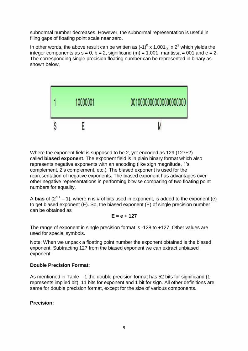
In other words, the above result can be written as (-1)0 x 1.001(2) x 22 which yields the integer components as s = 0, b = 2, significand (m) = 1.001, mantissa = 001 and e = 2. The corresponding single precision floating number can be represented in binary as shown below,

Where the exponent field is supposed to be 2, yet encoded as 129 (127+2) called biased exponent. The exponent field is in plain binary format which also represents negative exponents with an encoding (like sign magnitude, 1‘s complement, 2‘s complement, etc.). The biased exponent is used for the representation of negative exponents. The biased exponent has advantages over other negative representations in performing bitwise comparing of two floating point numbers for equality. A bias of (2n-1 – 1), where n is # of bits used in exponent, is added to the exponent (e) to get biased exponent (E). So, the biased exponent (E) of single precision number can be obtained as

E = e + 127

The range of exponent in single precision format is -128 to +127. Other values are used for special symbols.

Note: When we unpack a floating point number the exponent obtained is the biased exponent. Subtracting 127 from the biased exponent we can extract unbiased exponent. Double Precision Format: As mentioned in Table – 1 the double precision format has 52 bits for significand (1 represents implied bit), 11 bits for exponent and 1 bit for sign. All other definitions are same for double precision format, except for the size of various components.

Precision:

10

The smallest change that can be represented in floating point representation is called as precision. The fractional part of a single precision normalized number has exactly 23 bits of resolution, (24 bits with the implied bit). This corresponds to log(10) (2

23) = 6.924 = 7 (the characteristic of logarithm) decimal digits of accuracy. Similarly, in case of double precision numbers the precision is log(10) (2

52) = 15.654 = 16 decimal digits. Accuracy: Accuracy in floating point representation is governed by number of significand bits, whereas range is limited by exponent. Not all real numbers can exactly be represented in floating point format. For any numberwhich is not floating point number, there are two options for floating point approximation, say, the closest floating point number less than x as x_ and the closest floating point number greater than x as x+. A rounding operation is performed on number of significant bits in the mantissa field based on the selected mode. The round down mode causes x set to x_, the round up mode causes x set to x+, the round towards zero mode causes x is either x_ or x+ whichever is between zero and. The round to nearest mode sets x to x_ or x+ whichever is nearest to x. Usually round to nearest is most used mode. The closeness of floating point representation to the actual value is called as accuracy. Special Bit Patterns: The standard defines few special floating point bit patterns. Zero can‘t have most significant 1 bit, hence can‘t be normalized. The hidden bit representation requires a special technique for storing zero. We will have two different bit patterns +0 and -0 for the same numerical value zero. For single precision floating point representation, these patterns are given below,

0 00000000 00000000000000000000000 = +0

1 00000000 00000000000000000000000 = -0

Similarly, the standard represents two different bit patters for +INF and -INF. The same are given below,

0 11111111 00000000000000000000000 = +INF

1 11111111 00000000000000000000000 = -INF

All of these special numbers, as well as other special numbers (below) are subnormal numbers, represented through the use of a special bit pattern in the exponent field. This slightly reduces the exponent range, but this is quite acceptable since the range is so large.

An attempt to compute expressions like 0 x INF, 0 ÷ INF, etc. make no mathematical sense. The standard calls the result of such expressions as Not a Number (NaN). Any subsequent expression with NaN yields NaN. The representation of NaN has non-zero significand and all 1s in the exponent field. These are shown below for single precision format (x is don‘t care bits),

x 11111111 1m0000000000000000000000

11

Where m can be 0 or 1. This gives us two different representations of NaN. 0 11111111 110000000000000000000000 _____________ Signaling NaN (SNaN)

0 11111111 100000000000000000000000 _____________Quiet NaN (QNaN)

Usually QNaN and SNaN are used for error handling. QNaN do not raise any exceptions as they propagate through most operations. Whereas SNaN are which when consumed by most operations will raise an invalid exception.

Overflow and Underflow: Overflow is said to occur when the true result of an arithmetic operation is finite but larger in magnitude than the largest floating point number which can be stored using the given precision. Underflow is said to occur when the true result of an arithmetic operation is smaller in magnitude (infinitesimal) than the smallest normalized floating point number which can be stored. Overflow can‘t be ignored in calculations whereas underflow can effectively be replaced by zero. Endianness: The IEEE 754 standard defines a binary floating point format. The architecture details are left to the hardware manufacturers. The storage order of individual bytes in binary floating point numbers varies from architecture to architecture.

Errors in numerical computation

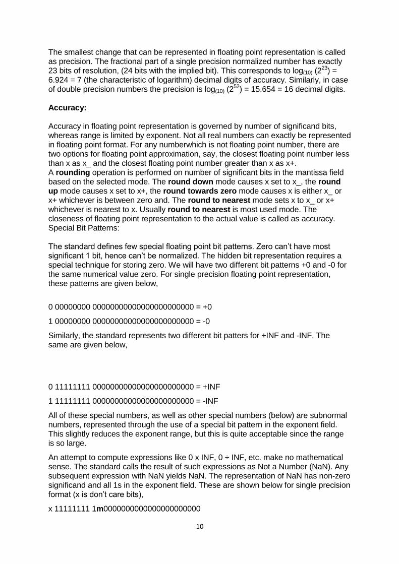
Many engineering problems are too time consuming to solve or may not be able to be solved analytically. In these situations, numerical methods are usually employed. Numerical methods are techniques designed to solve a problem using numerical approximations. An example of an application of numerical methods is trying to determine the velocity of a falling object. If you know the exact function that determines the position of your object, then you could potentially differentiate the function to obtain an expression for the velocity. More often, you will use a machine to record readings of times and positions that you can then use to numerically solve for velocity:

where f is your function, t is the time of the reading, and h is the distance to the next time step. Because your answer is an approximation of the analytical solution, there is an inherent error between the approximated answer and the exact solution. Errors can result prior to computation in the form of measurement errors or assumptions in modeling. The focus of this blog post will be on understanding two types of errors that can occur during computation: roundoff errors and truncation errors.

12

Roundoff Error

Roundoff errors occur because computers have a limited ability to represent numbers. For example, π has infinite digits, but due to precision limitations, only 16 digits may be stored in MATLAB. While this roundoff error may seem insignificant, if your process involves multiple iterations that are dependent on one another, these small errors may accumulate over time and result in a significant deviation from the expected value. Furthermore, if a manipulation involves adding a large and small number, the effect of the smaller number may be lost if rounding is utilized. Thus, it is advised to sum numbers of similar magnitudes first so that smaller numbers are not ―lost‖ in the calculation.

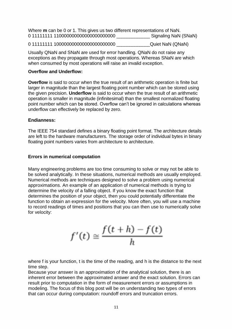
One interesting example that we covered in my Engineering Computation class, that can be used to illustrate this point, involves the quadratic formula. The quadratic formula is represented as follows:

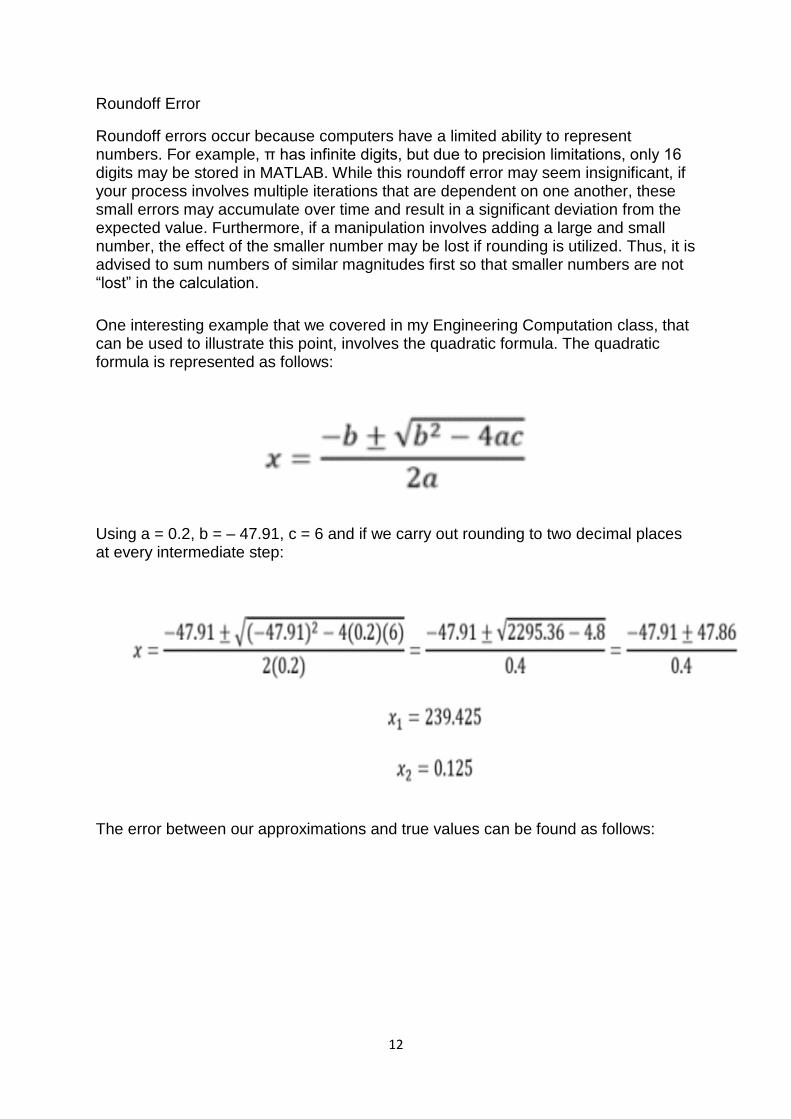
Using a = 0.2, b = – 47.91, c = 6 and if we carry out rounding to two decimal places at every intermediate step:

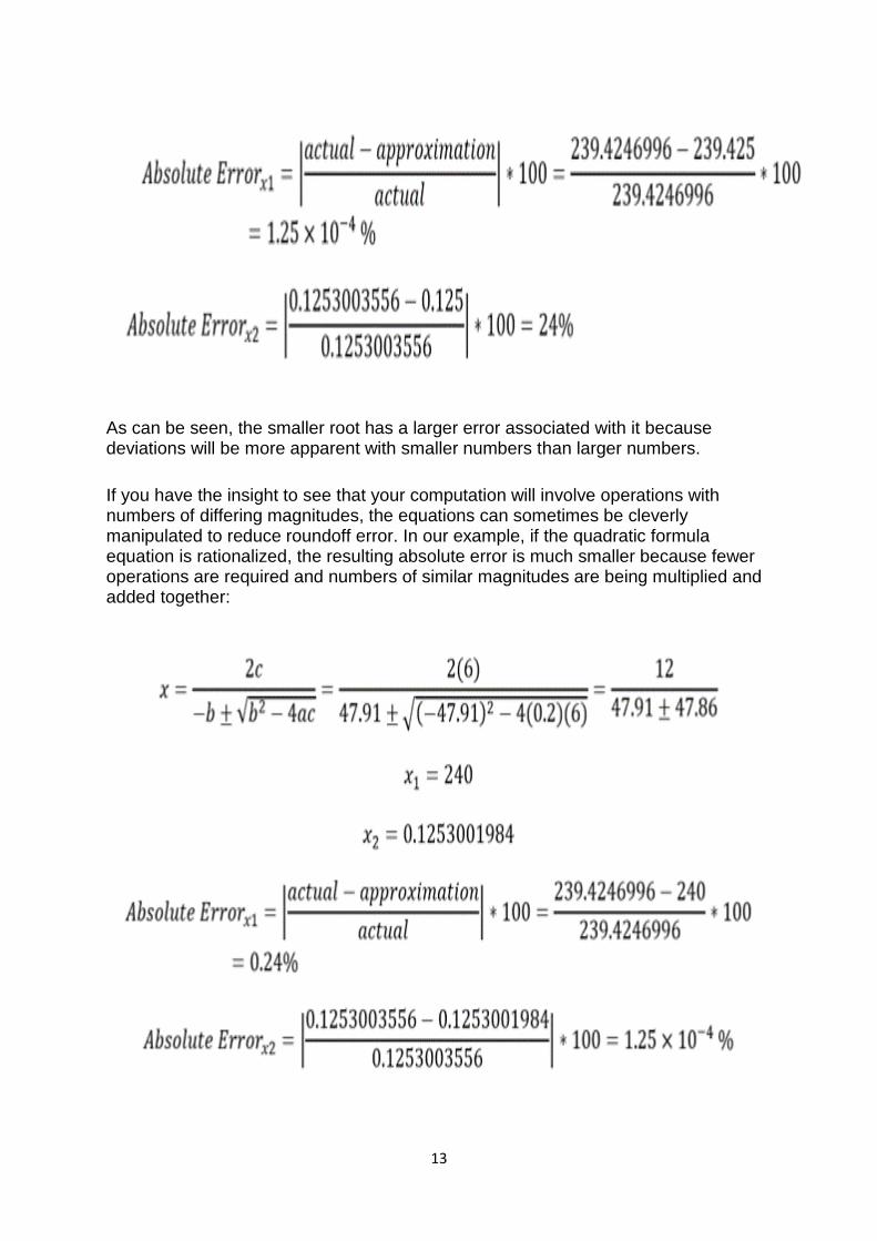
The error between our approximations and true values can be found as follows:

13

As can be seen, the smaller root has a larger error associated with it because deviations will be more apparent with smaller numbers than larger numbers.

If you have the insight to see that your computation will involve operations with numbers of differing magnitudes, the equations can sometimes be cleverly manipulated to reduce roundoff error. In our example, if the quadratic formula equation is rationalized, the resulting absolute error is much smaller because fewer operations are required and numbers of similar magnitudes are being multiplied and added together:

14

Truncation Error

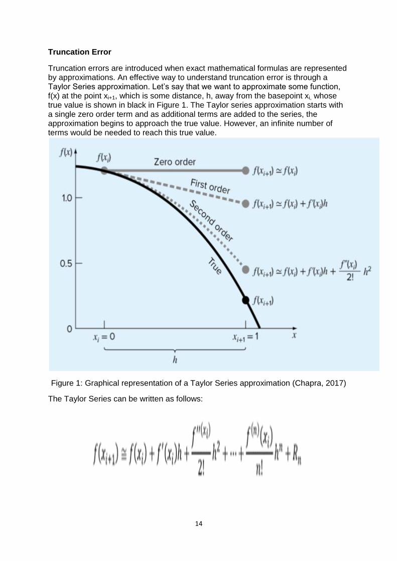
Truncation errors are introduced when exact mathematical formulas are represented by approximations. An effective way to understand truncation error is through a Taylor Series approximation. Let‘s say that we want to approximate some function, f(x) at the point xi+1, which is some distance, h, away from the basepoint xi, whose true value is shown in black in Figure 1. The Taylor series approximation starts with a single zero order term and as additional terms are added to the series, the approximation begins to approach the true value. However, an infinite number of terms would be needed to reach this true value.

Figure 1: Graphical representation of a Taylor Series approximation (Chapra, 2017)

The Taylor Series can be written as follows:

15

where Rn is a remainder term used to account for all of the terms that were not included in the series and is therefore a representation of the truncation error. The remainder term is generally expressed as Rn=O(hn+1) which shows that truncation error is proportional to the step size, h, raised to the n+1 where n is the number of terms included in the expansion. It is clear that as the step size decreases, so does the truncation error. The Tradeoff in Errors

The total error of an approximation is the summation of roundoff error and truncation error. As seen from the previous sections, truncation error decreases as step size decreases. However, when step size decreases, this usually results in the necessity for more precise computations which consequently results in an increase in roundoff error. Therefore, the errors are in direct conflict with one another: as we decrease one, the other increases.

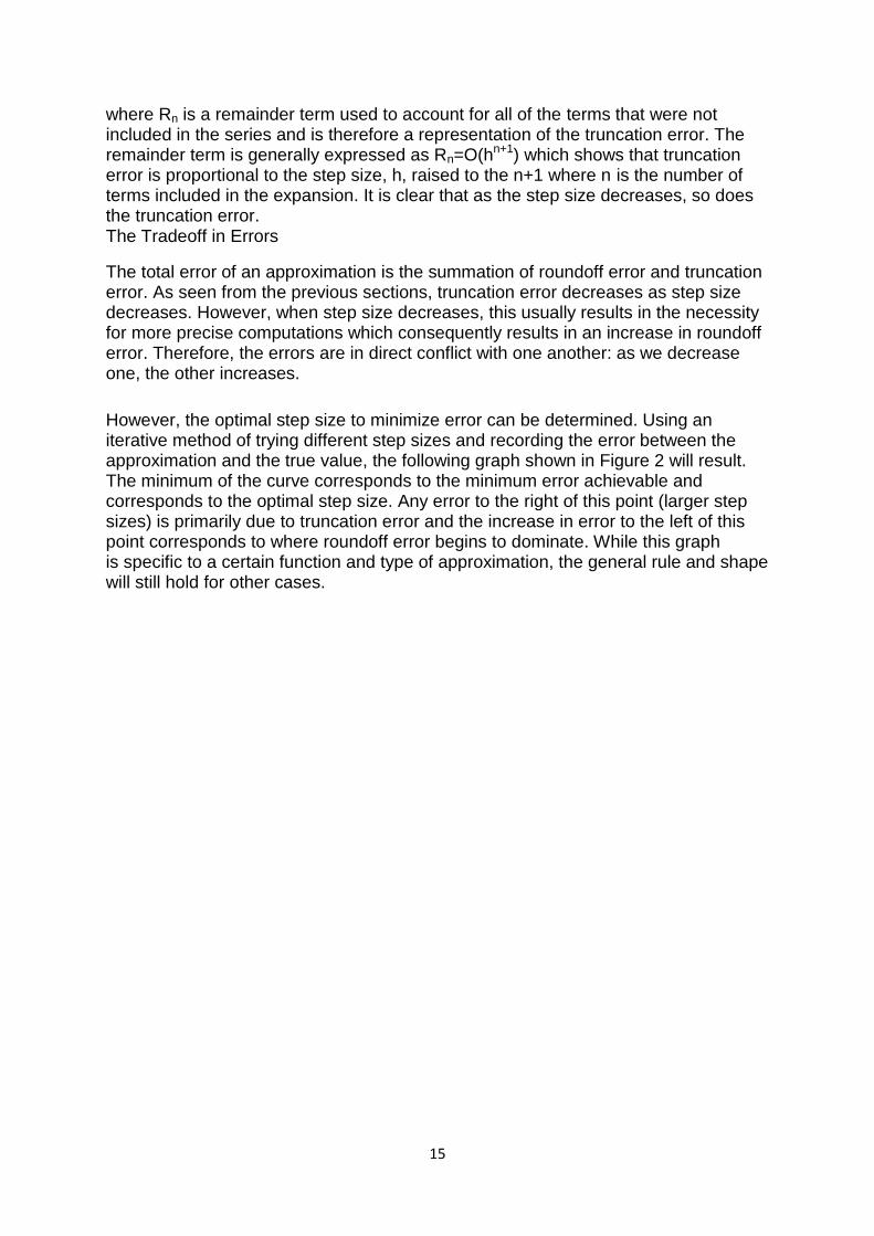
However, the optimal step size to minimize error can be determined. Using an iterative method of trying different step sizes and recording the error between the approximation and the true value, the following graph shown in Figure 2 will result. The minimum of the curve corresponds to the minimum error achievable and corresponds to the optimal step size. Any error to the right of this point (larger step sizes) is primarily due to truncation error and the increase in error to the left of this point corresponds to where roundoff error begins to dominate. While this graph is specific to a certain function and type of approximation, the general rule and shape will still hold for other cases.

16

Figure 2: Plot of Error vs. Step Size (Chapra, 2017)

Hopefully this blog post was helpful to increase awareness of the types of errors that you may come across when using numerical methods! Internalize these golden rules to help avoid loss of significance:

Avoid subtracting two nearly equal numbers

If your equation has large and small numbers, work with smaller numbers first

Consider rearranging your equation so that numbers of a similar magnitude are being used in an operation

17

UNIT-II

Iterative Methods

Zeros of a single transcendental equation and zeros of polynomial using

Bisection Method,

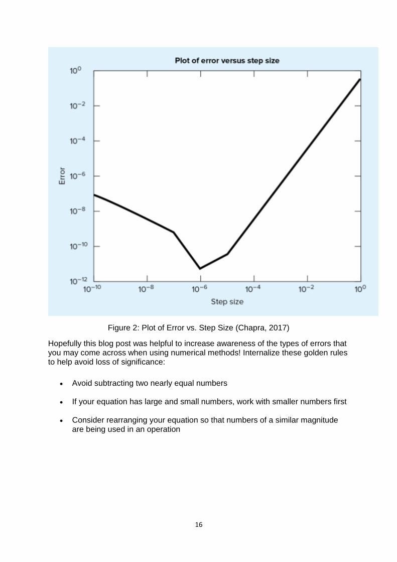
Bisection method is the simplest among all the numerical schemes to solve the

transcendental equations. This scheme is based on the intermediate value theorem

for continuous functions .

Consider a transcendental equation f (x) = 0 which has a zero in the interval [a,b] and f (a) * f (b) < 0. Bisection scheme computes the zero, say c, by repeatedly halving the interval [a,b]. That is, starting with

c = (a+b) / 2

the interval [a,b] is replaced either with [c,b] or with [a,c] depending on the sign of f (a) * f (c) . This process is continued until the zero is obtained. Since the zero is obtained numerically the value of c may not exactly match with all the decimal places of the analytical solution of f (x) = 0 in the interval [a,b]. Hence any one of the following mechanisms can be used to stop the bisection iterations :

interval or the maximum error after N iterations in this case is less than | b-a | / 2N.

ng the condition | ci - c i-1| (where i are the iteration number) less than some tolerance limit, say epsilon, fixed a priori.

i ) | less than some tolerance limit alpha again fixed a priori.

Algorithm - Bisection Scheme

Given a function f (x) continuous on an interval [a,b] and f (a) * f (b) < 0 Do c = (a+b)/2 if f (a) * f (c) < 0 then b = c else a = c while (none of the convergence criteria C1, C2 or C3 is satisfied)

18

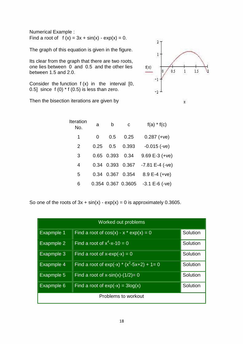
Numerical Example :

Find a root of f (x) = 3x + sin(x) - exp(x) = 0.

The graph of this equation is given in the figure.

Its clear from the graph that there are two roots, one lies between 0 and 0.5 and the other lies between 1.5 and 2.0.

Consider the function f (x) in the interval [0, 0.5] since f (0) * f (0.5) is less than zero.

Then the bisection iterations are given by

Iteration

No. a b c f(a) * f(c)

1 0 0.5 0.25 0.287 (+ve)

2 0.25 0.5 0.393 -0.015 (-ve)

3 0.65 0.393 0.34 9.69 E-3 (+ve)

4 0.34 0.393 0.367 -7.81 E-4 (-ve)

5 0.34 0.367 0.354 8.9 E-4 (+ve)

6 0.354 0.367 0.3605 -3.1 E-6 (-ve)

So one of the roots of 3x + sin(x) - exp(x) = 0 is approximately 0.3605.

Worked out problems

Exapmple 1 Find a root of cos(x) - x * exp(x) = 0 Solution

Exapmple 2 Find a root of x4-x-10 = 0 Solution

Exapmple 3 Find a root of x-exp(-x) = 0 Solution

Exapmple 4 Find a root of exp(-x) * (x2-5x+2) + 1= 0 Solution

Exapmple 5 Find a root of x-sin(x)-(1/2)= 0 Solution

Exapmple 6 Find a root of exp(-x) = 3log(x) Solution

Problems to workout

19

Iteration Method

Considerable attention has been devoted to the study of the fractional calculus

during the past three decades and its numerous applications in the area of physics

and engineering. The applications of fractional calculus used in many fields such as

electrical networks, control theory of dynamical systems, probability and statistics,

electrochemistry, chemical physics, optics, and signal processing can be

successfully modelled by linear or nonlinear fractional differential equations.

So far there have been several fundamental works on the fractional derivative and

fractional differential equations [1–3]. These works are to be considered as an

introduction to the theory of fractional derivative and fractional differential equations

and provide a systematic understanding of the fractional calculus such as the

existence and uniqueness [4, 5]. Recently, many other researchers have paid

attention to existence result of solution of the initial value problem and boundary

problem for fractional differential equations [4–6].

Finding approximate or exact solutions of fractional differential equations is an

important task. Except for a limited number of these equations, we have difficulty in

finding their analytical solutions. Therefore, there have been attempts to develop

new methods for obtaining analytical solutions which reasonably approximate the

exact solutions. Several such techniques have drawn special attention, such as

Adomain‘s decomposition method [7], homotopy perturbation method [8–10],

homotopy analysis method [11, 12], variational iteration method [13–17], Chebyshev

spectral method [18, 19], and new iterative method [20–22]. Among them, the new

iterative method provides an effective procedure for explicit and numerical solutions

of a wide and general class of differential systems representing real physical

problems. The new iterative method is more superior than the other nonlinear

methods, such as the perturbation methods where this method does not depend on

small parameters, such that it can find wide application in nonlinear problems without

linearization or small perturbation.

The motivation of this paper is to extend the application of the new iterative method

proposed by Daftardar-Gejji and Jafari [20–22] to solve linear and nonlinear ordinary

and partial differential equations of fractional order. This motivation is based on the

importance of these equations and their applications in various subjects in physical

branches [10, 11, 14, 23–25].

There are several definitions of a fractional derivative of order [3, 26]. The two most

commonly used definitions are Riemann-Liouville and Caputo. Each definition uses

Riemann-Liouville fractional integration and derivative of whole order. The difference

between the two definitions is in the order of evaluation. Riemann-Liouville fractional

integration of order is defined asThe next two equations define Riemann-Liouville

and Caputo fractional derivatives of order ,  respectively, aswhere ,  .

Caputo fractional derivative first computes an ordinary derivative followed by a

fractional integral to achieve the desired order of fractional derivative. Riemann-

Liouville fractional derivative is computed in the reverse order. Therefore, Caputo

20

fractional derivative allows traditional initial and boundary conditions to be included in

the formulation of the problem.

From properties of   and ,  it is important to note thatwhere   is Caputo derivative

operator of order ,

2. Basic Idea of New Iterative Method

For the basic idea of the new iterative method, we consider the following general

functional equation [20–22]:where is a nonlinear operator from a Banach

space and   is a known function. We have been looking for a solution of (4) having

the series formThe nonlinear operator can be decomposed asFrom (5) and (6), (4)

is equivalent toWe define the following recurrence relation:Then,If ,  , thenand the

series absolutely and uniformly converges to a solution of (4) [27], which is unique,

in view of the Banach fixed point theorem [28]. The n-term approximate solution of

(4) and (5) is given by

2.1. Convergence of the Method

Now we analyze the convergence of the new iterative method for solving any general

functional equation (4). Let , where is the exact solution, is the approximate

solution, and is the error in the solution of (4); obviously satisfies (4), that is,and the

recurrence relation (8) becomesIf ,  , thenThus as , which proves the convergence of

the new iterative method for solving the general functional equation (4). For more

details, you can see [29].

3. Suitable Algorithm

In this section, we introduce a suitable algorithm for solving nonlinear partial

differential equations using the new iterative method. Consider the following

nonlinear partial differential equation of arbitrary order:where is a nonlinear function

of and (partial derivatives of with respect to and ) and is the source function. In

view of the new iterative method, the initial value problem (14a) and (14b) is

equivalent to the integral equationwhere

Remark 1. When the general functional equation (4) is linear, the recurrence relation

(8) can be simplified in the form

Proof. From the properties of integration and by using (8) and (16b), we

haveTherefore, we get the solution of (15) by employing the recurrence relation (8)

or (17).

21

4. Applications

To illustrate the effectiveness of the proposed method, several test examples are

carried out in this section.

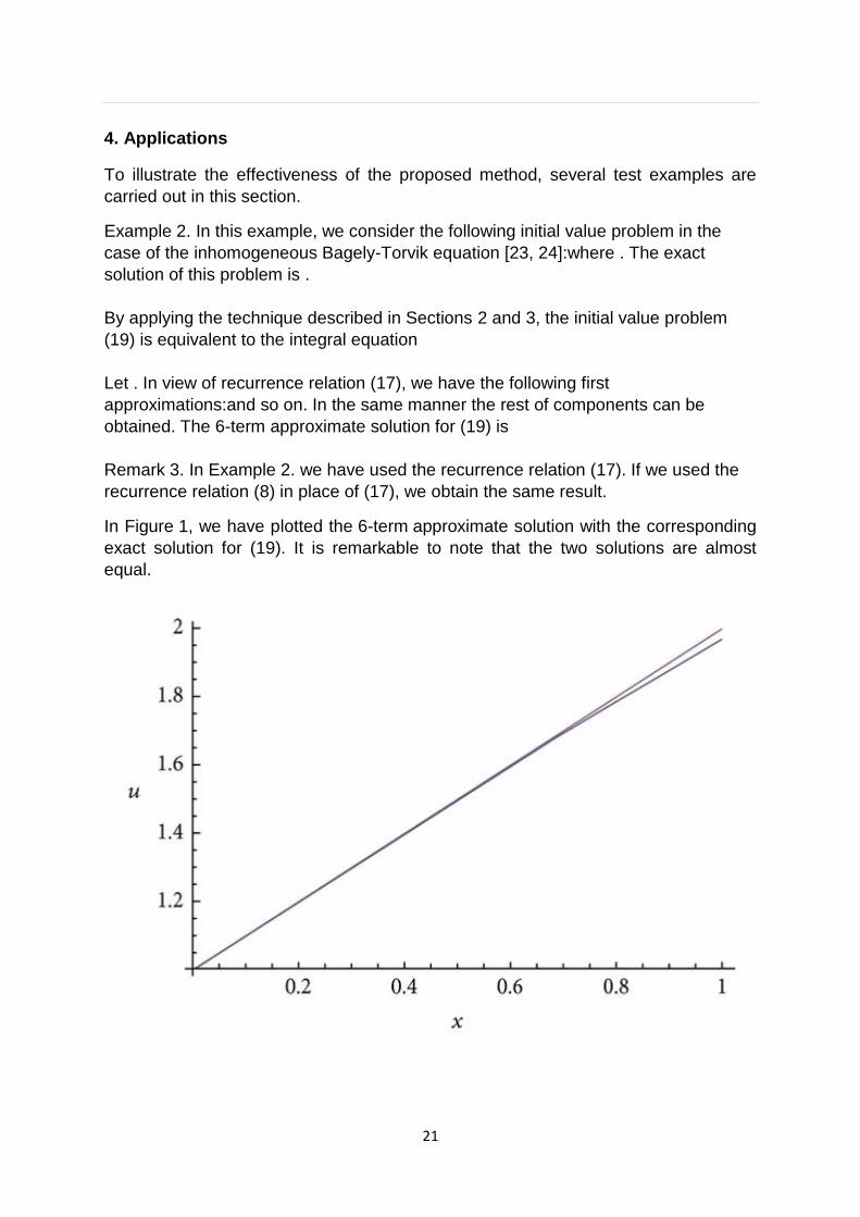
Example 2. In this example, we consider the following initial value problem in the

case of the inhomogeneous Bagely-Torvik equation [23, 24]:where . The exact

solution of this problem is .

By applying the technique described in Sections 2 and 3, the initial value problem

(19) is equivalent to the integral equation

Let . In view of recurrence relation (17), we have the following first

approximations:and so on. In the same manner the rest of components can be

obtained. The 6-term approximate solution for (19) is

Remark 3. In Example 2. we have used the recurrence relation (17). If we used the

recurrence relation (8) in place of (17), we obtain the same result.

In Figure 1, we have plotted the 6-term approximate solution with the corresponding

exact solution for (19). It is remarkable to note that the two solutions are almost

equal.

22

Figure 1

Plots of the approximate solution and the exact solution for (19).

Comparing these obtained results with those obtained by new Jacobi operational

matrix in [23, 24], we can confirm the simplicity and accuracy of the given method.

Example 4. Consider the following fractional Riccati equation [10]:The exact solution

when is .

By applying the technique described in Sections 2 and 3, the initial value problem

(23) is equivalent to the integral equation

Let . In view of recurrence relation (8), we have the following first approximations:and

so on. The 4-term approximate solution for (23) is

In Figure 2, we have plotted the 4-term approximate solution for (23) for different

values of with the corresponding exact solution. It is remarkable to note that the

approximate solution,  in case ,  and the exact solution are almost equal (continuous

curve) whenever the approximate solution, in cases , is of high agreement with the

exact solution (dashed and dotted curves, resp.).

Figure 2

Plots of the approximate solution for different values of and the exact solution for

(23).

23

Comparing the obtained results with those obtained by homotopy analysis method,

in case , in [10], we can confirm the simplicity and accuracy of the given method.

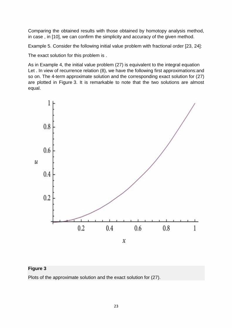
Example 5. Consider the following initial value problem with fractional order [23, 24]:

The exact solution for this problem is .

As in Example 4, the initial value problem (27) is equivalent to the integral equation

Let . In view of recurrence relation (8), we have the following first approximations:and

so on. The 4-term approximate solution and the corresponding exact solution for (27)

are plotted in Figure 3. It is remarkable to note that the two solutions are almost

equal.

Figure 3

Plots of the approximate solution and the exact solution for (27).

24

Comparing these obtained results with those obtained by new Jacobi operational

matrix in [23, 24], we can confirm the simplicity and accuracy of the given method.

Example 6. Consider the following fractional order wave equation in 2-

dimensional space [14]:

The exact solution for this problem when is

The initial value problem (30) is equivalent to the integral equation

Let .  In view of recurrence relation (17), we have the following first

approximations:and so on. The n-term approximate solution for (30) isIn closed form

this gives:which is the exact solution for the given problem. When , the above n-

term approximate solution for (30) becomesIn closed form, this giveswhich is the

same result obtained by variational iteration method in [14].

Example 7. Consider the following fractional order heat equation in 2-

dimensional space [11]:

The exact solution for this problem when is

The initial value problem (38) is equivalent to the integral equation

Let . In view of recurrence relation (17), we have the following first

approximations:and so on. The n-term approximate solution for (38) isWhen , The n-

term approximate solution for (38) becomesIn closed form, this giveswhich is the

exact solution for the given problem.

The obtained results in this example are the same as these obtained in [11] by the

homotopy perturbation method, in case , but with the simplicity of the given method.

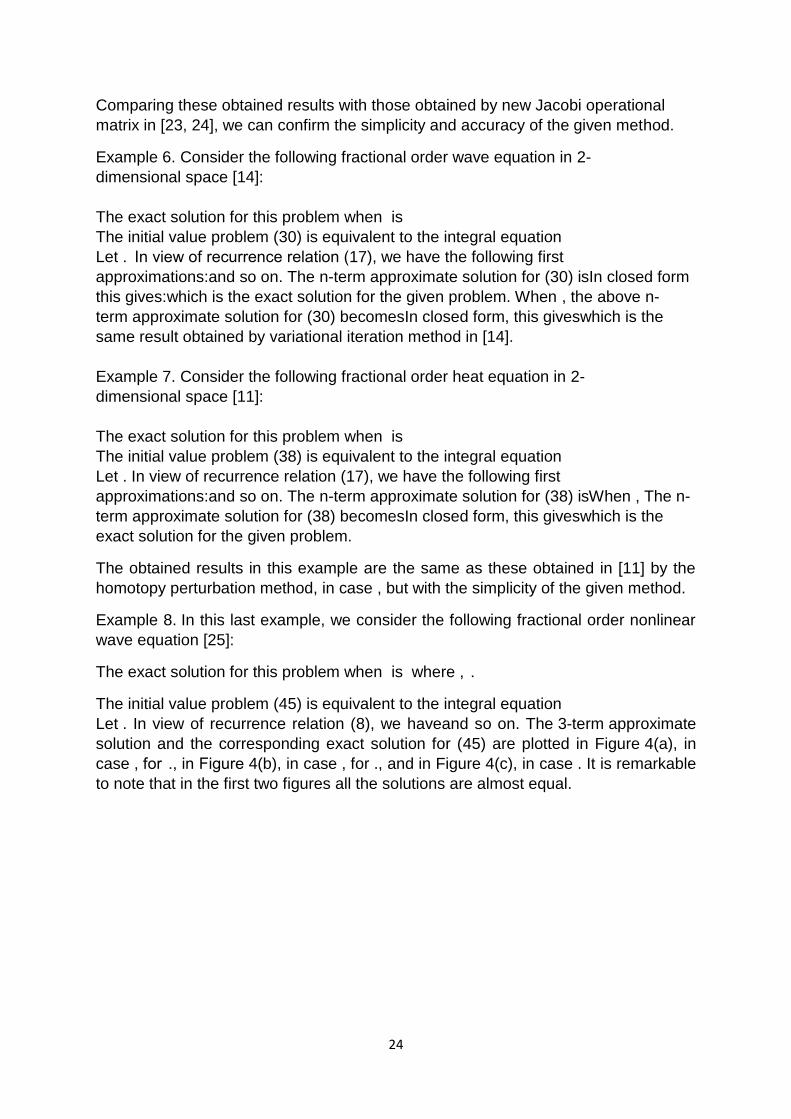
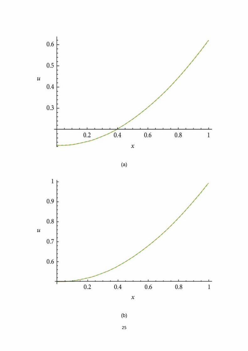
Example 8. In this last example, we consider the following fractional order nonlinear

wave equation [25]:

The exact solution for this problem when is where ,  .

The initial value problem (45) is equivalent to the integral equation

Let . In view of recurrence relation (8), we haveand so on. The 3-term approximate

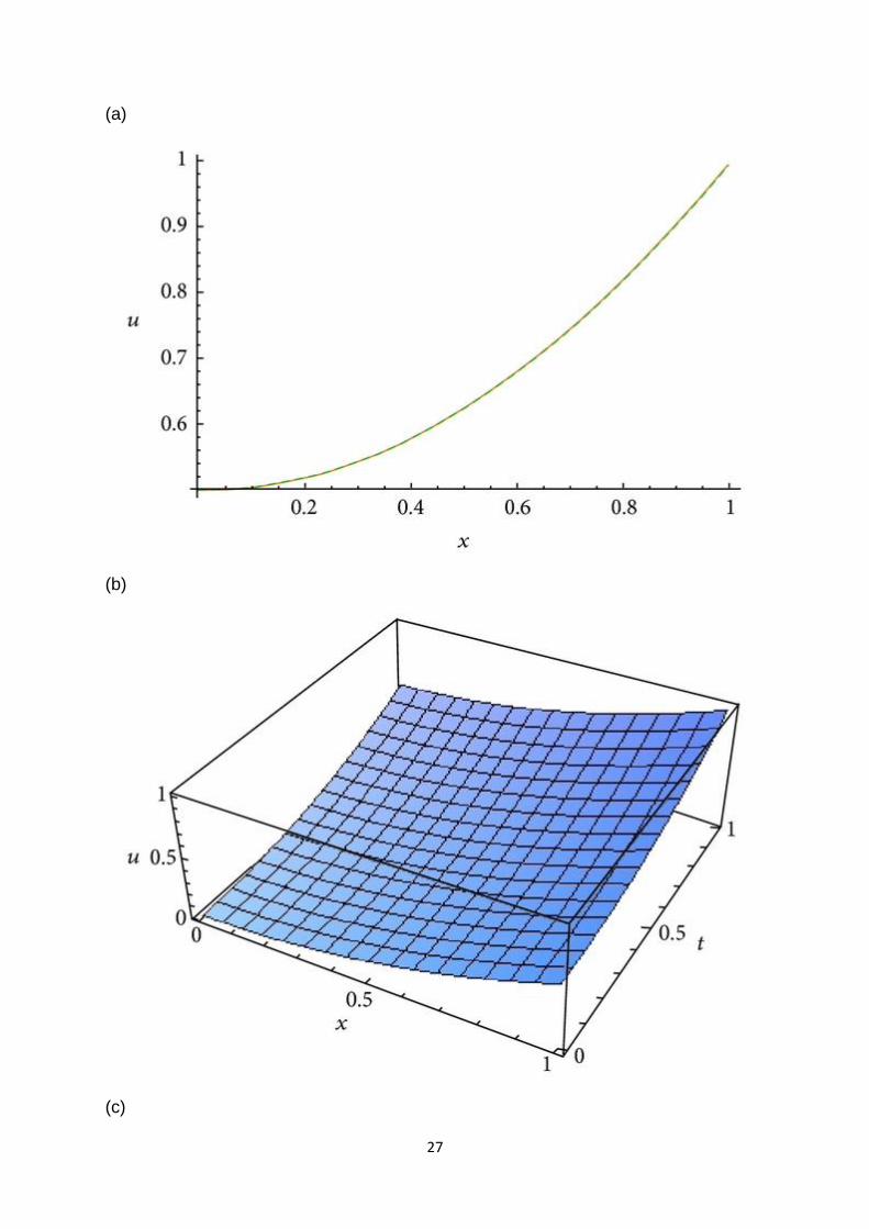
solution and the corresponding exact solution for (45) are plotted in Figure 4(a), in

case , for  ., in Figure 4(b), in case , for ., and in Figure 4(c), in case . It is remarkable

to note that in the first two figures all the solutions are almost equal.

25

(a)

(b)

26

(c)

27

(a)

(b)

(c)

28

Figure 4

(a) Plots of the approximate solution for different values of and the exact solution, in

case ; for (45). (b) Plots of the approximate solution for different values of and the

exact solution, in case ; for (45). (c) Plots of the approximate solution, in case for

(45).

Comparing these results with those obtained by the modification homotopy

perturbation method in [25], we can confirm the accuracy and simplicity of the given

method.

5. Conclusion

In this paper, the new iterative method with suitable algorithm is successfully used to

solve linear and nonlinear ordinary and partial differential equations with fractional

order. It is clear that the computations are easy and the solutions agree well with the

corresponding exact solutions and more accurate than the solutions obtained by

other methods. Moreover, the accuracy is high with little computed terms of the

solution which confirm that this method with the given algorithm is a powerful method

for handling fractional differential equations.

Regula-Falsi method

The Regula–Falsi Method is a numerical method for estimating the roots of a polynomial f(x). A value x replaces the midpoint in the Bisection Method and serves as the new approximation of a root of f(x). The objective is to make convergence faster. Assume that f(x) is continuous.

Algorithm for the Regula–Falsi Method: Given a continuous function f(x)

1. Find points a and b such that a < b and f(a) * f(b) < 0.

2. Take the interval [a, b] and determine the next value of x1.

3. If f(x1) = 0 then x1 is an exact root, else if f(x1) * f(b) < 0 then let a = x1, else if f(a) * f(x1) < 0 then let b = x1.

4. Repeat steps 2 & 3 until f(xi) = 0 or |f(xi)| £ DOA, where DOA stands for degree of accuracy.

29

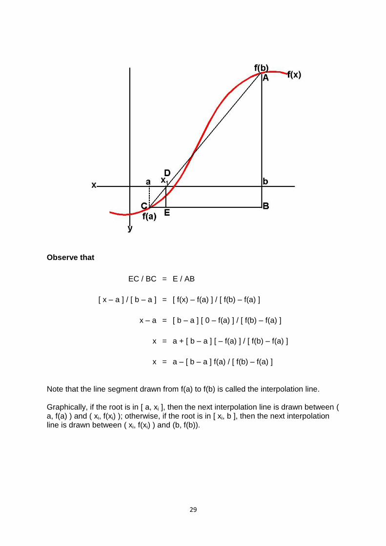
Observe that

EC / BC = E / AB

[ x – a ] / [ b – a ] = [ f(x) – f(a) ] / [ f(b) – f(a) ]

x – a = [ b – a ] [ 0 – f(a) ] / [ f(b) – f(a) ]

x = a + [ b – a ] [ – f(a) ] / [ f(b) – f(a) ]

x = a – [ b – a ] f(a) / [ f(b) – f(a) ]

Note that the line segment drawn from f(a) to f(b) is called the interpolation line.

Graphically, if the root is in [ a, xi ], then the next interpolation line is drawn between ( a, f(a) ) and ( xi, f(xi) ); otherwise, if the root is in [ xi, b ], then the next interpolation line is drawn between ( xi, f(xi) ) and (b, f(b)).

30

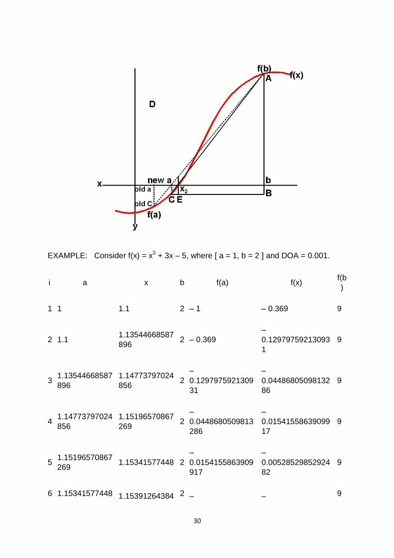
EXAMPLE: Consider f(x) = x3 + 3x – 5, where [ a = 1, b = 2 ] and DOA = 0.001.

i a x b f(a) f(x) f(b

)

1 1 1.1 2 – 1 – 0.369 9

2 1.1 1.13544668587

896 2 – 0.369

–

0.12979759213093

1

9

3 1.13544668587

896

1.14773797024

856 2

–

0.1297975921309

31

–

0.04486805098132

86

9

4 1.14773797024

856

1.15196570867

269 2

–

0.0448680509813

286

–

0.01541558639099

17

9

5 1.15196570867

269 1.15341577448 2

–

0.0154155863909

917

–

0.00528529852924

82

9

6 1.15341577448 1.15391264384 2 – – 9

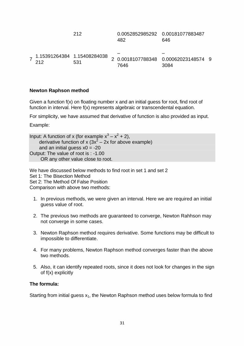
31

212 0.0052852985292

482

0.00181077883487

646

7 1.15391264384

212

1.15408284038

531 2

–

0.0018107788348

7646

–

0.00062023148574

3084

9

Newton Raphson method

Given a function f(x) on floating number x and an initial guess for root, find root of function in interval. Here f(x) represents algebraic or transcendental equation.

For simplicity, we have assumed that derivative of function is also provided as input.

Example: Input: A function of x (for example x3 – x2 + 2), derivative function of x (3x2 – 2x for above example) and an initial guess x0 = -20 Output: The value of root is : -1.00 OR any other value close to root. We have discussed below methods to find root in set 1 and set 2 Set 1: The Bisection Method Set 2: The Method Of False Position Comparison with above two methods:

1. In previous methods, we were given an interval. Here we are required an initial guess value of root.

2. The previous two methods are guaranteed to converge, Newton Rahhson may not converge in some cases.

3. Newton Raphson method requires derivative. Some functions may be difficult to impossible to differentiate.

4. For many problems, Newton Raphson method converges faster than the above two methods.

5. Also, it can identify repeated roots, since it does not look for changes in the sign of f(x) explicitly

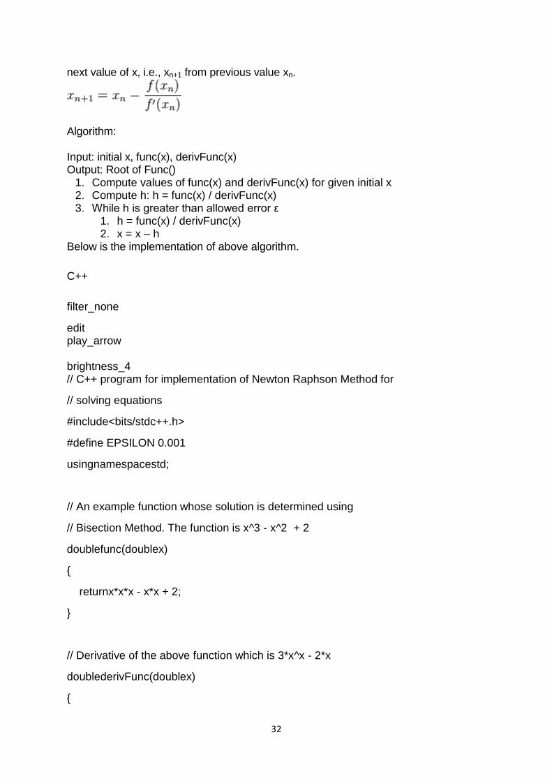
The formula: Starting from initial guess x1, the Newton Raphson method uses below formula to find

32

next value of x, i.e., xn+1 from previous value xn.

Algorithm: Input: initial x, func(x), derivFunc(x) Output: Root of Func()

1. Compute values of func(x) and derivFunc(x) for given initial x 2. Compute h: h = func(x) / derivFunc(x) 3. While h is greater than allowed error ε

1. h = func(x) / derivFunc(x) 2. x = x – h

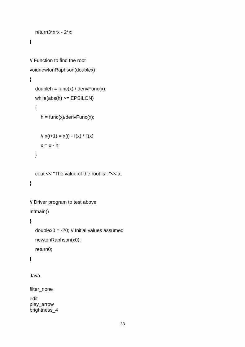
Below is the implementation of above algorithm.

C++

filter_none

edit play_arrow brightness_4 // C++ program for implementation of Newton Raphson Method for

// solving equations

#include<bits/stdc++.h>

#define EPSILON 0.001

usingnamespacestd;

// An example function whose solution is determined using

// Bisection Method. The function is x^3 - x^2 + 2

doublefunc(doublex)

{

returnx*x*x - x*x + 2;

}

// Derivative of the above function which is 3*x^x - 2*x

doublederivFunc(doublex)

{

33

return3*x*x - 2*x;

}

// Function to find the root

voidnewtonRaphson(doublex)

{

doubleh = func(x) / derivFunc(x);

while(abs(h) >= EPSILON)

{

h = func(x)/derivFunc(x);

// x(i+1) = x(i) - f(x) / f'(x)

x = x - h;

}

cout << "The value of the root is : "<< x;

}

// Driver program to test above

intmain()

{

doublex0 = -20; // Initial values assumed

newtonRaphson(x0);

return0;

}

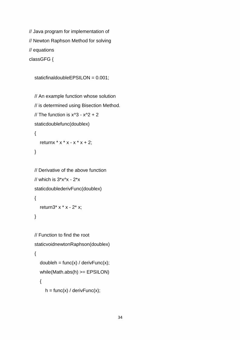
Java

filter_none

edit play_arrow brightness_4

34

// Java program for implementation of

// Newton Raphson Method for solving

// equations

classGFG {

staticfinaldoubleEPSILON = 0.001;

// An example function whose solution

// is determined using Bisection Method.

// The function is x^3 - x^2 + 2

staticdoublefunc(doublex)

{

returnx * x * x - x * x + 2;

}

// Derivative of the above function

// which is 3*x^x - 2*x

staticdoublederivFunc(doublex)

{

return3* x * x - 2* x;

}

// Function to find the root

staticvoidnewtonRaphson(doublex)

{

doubleh = func(x) / derivFunc(x);

while(Math.abs(h) >= EPSILON)

{

h = func(x) / derivFunc(x);

35

// x(i+1) = x(i) - f(x) / f'(x)

x = x - h;

}

System.out.print("The value of the"

+ " root is : "

+ Math.round(x * 100.0) / 100.0);

}

// Driver code

publicstaticvoidmain (String[] args)

{

// Initial values assumed

doublex0 = -20;

newtonRaphson(x0);

}

}

// This code is contributed by Anant Agarwal.

Python3

filter_none

edit play_arrow brightness_4 # Python3 code for implementation of Newton

# Raphson Method for solving equations

# An example function whose solution

# is determined using Bisection Method.

36

# The function is x^3 - x^2 + 2

deffunc( x ):

returnx *x *x -x *x +2

# Derivative of the above function

# which is 3*x^x - 2*x

defderivFunc( x ):

return3*x *x -2*x

# Function to find the root

defnewtonRaphson( x ):

h =func(x) /derivFunc(x)

whileabs(h) >=0.0001:

h =func(x)/derivFunc(x)

# x(i+1) = x(i) - f(x) / f'(x)

x =x -h

print("The value of the root is : ",

"%.4f"%x)

# Driver program to test above

x0 =-20# Initial values assumed

newtonRaphson(x0)

# This code is contributed by "Sharad_Bhardwaj"

C#

filter_none

edit play_arrow

37

brightness_4 // C# program for implementation of

// Newton Raphson Method for solving

// equations

usingSystem;

classGFG {

staticdoubleEPSILON = 0.001;

// An example function whose solution

// is determined using Bisection Method.

// The function is x^3 - x^2 + 2

staticdoublefunc(doublex)

{

returnx * x * x - x * x + 2;

}

// Derivative of the above function

// which is 3*x^x - 2*x

staticdoublederivFunc(doublex)

{

return3 * x * x - 2 * x;

}

// Function to find the root

staticvoidnewtonRaphson(doublex)

{

doubleh = func(x) / derivFunc(x);

while(Math.Abs(h) >= EPSILON)

{

38

h = func(x) / derivFunc(x);

// x(i+1) = x(i) - f(x) / f'(x)

x = x - h;

}

Console.Write("The value of the"

+ " root is : "

+ Math.Round(x * 100.0) / 100.0);

}

// Driver code

publicstaticvoidMain ()

{

// Initial values assumed

doublex0 = -20;

newtonRaphson(x0);

}

}

// This code is contributed by nitin mittal

PHP

filter_none

edit play_arrow brightness_4 <?php

// PHP program for implementation

// of Newton Raphson Method for

39

// solving equations

$EPSILON= 0.001;

// An example function whose

// solution is determined

// using Bisection Method.

// The function is x^3 - x^2 + 2

functionfunc($x)

{

return$x* $x* $x-

$x* $x+ 2;

}

// Derivative of the above

// function which is 3*x^x - 2*x

functionderivFunc($x)

{

return3 * $x*

$x- 2 * $x;

}

// Function to

// find the root

functionnewtonRaphson($x)

{

global$EPSILON;

$h= func($x) / derivFunc($x);

while(abs($h) >= $EPSILON)

{

$h= func($x) / derivFunc($x);

40

// x(i+1) = x(i) -

// f(x) / f'(x)

$x= $x- $h;

}

echo"The value of the ".

"root is : ", $x;

}

// Driver Code

$x0= -20; // Initial values assumed

newtonRaphson($x0);

// This code is contributed by ajit

?>

Output:

The value of root is : -1.00

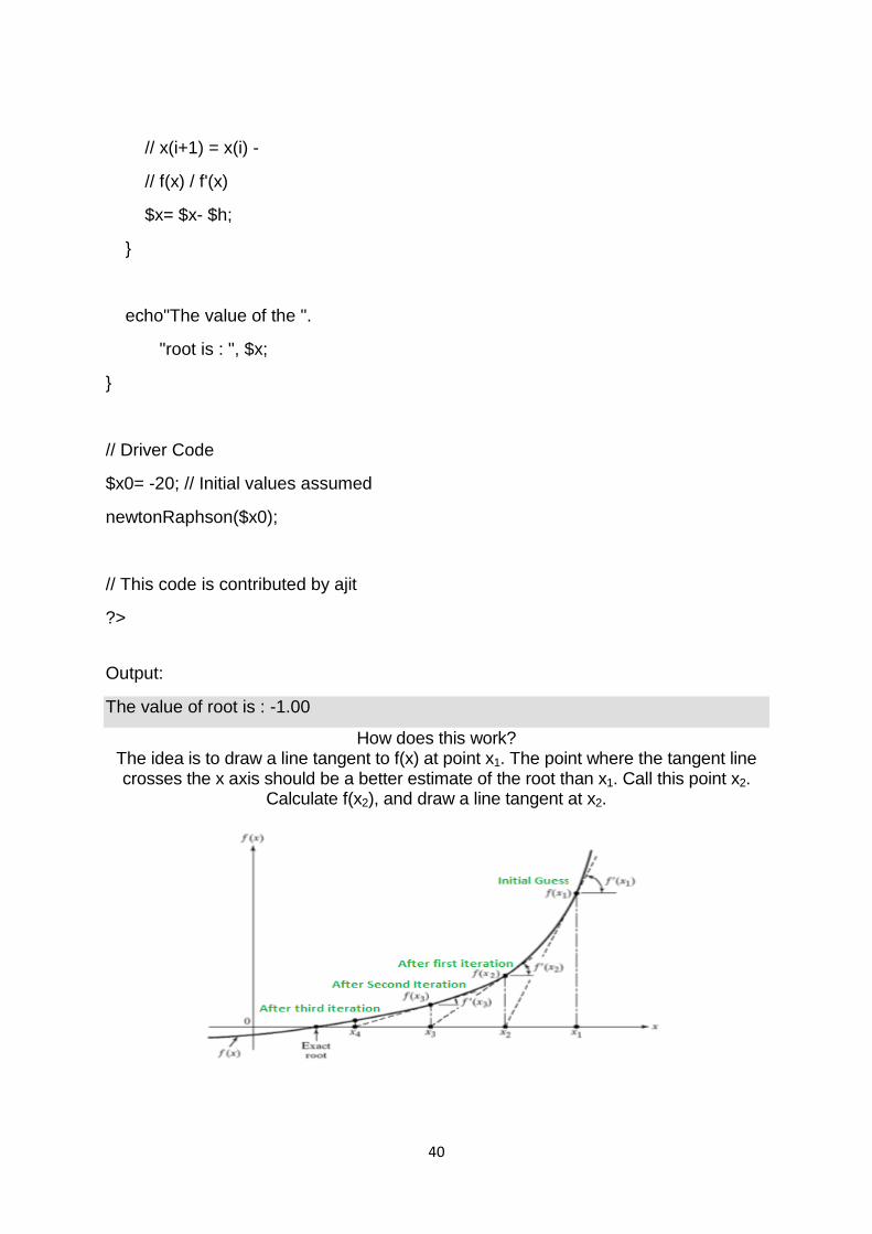
How does this work? The idea is to draw a line tangent to f(x) at point x1. The point where the tangent line crosses the x axis should be a better estimate of the root than x1. Call this point x2.

Calculate f(x2), and draw a line tangent at x2.

41

We know that slope of line from (x1, f(x1)) to (x2, 0) is f'(x1)) where f‘ represents derivative of f.

f'(x1) = (0 - f(x1)) / (x2 - x1) f'(x1) * (x2 - x1) = - f(x1) x2 = x1 - f(x1) / f'(x1) By finding this point 'x2', we move closer towards the root. We have to keep on repeating the above step till we get really close to the root or we find it. In general, xn+1 = xn - f(xn) / f'(xn) Alternate Explanation using Taylor‘s Series: Let x1 be the initial guess. We can write x2 as below: xn+1 = xn + h ------- (1) Here h would be a small value that can be positive or negative. According to Taylor's Series, ƒ(x) that is infinitely differentiable can be written as below f(xn+1) = f(xn + h) = f(xn) + h*f'(xn) + ((h*h)/2!)*(f''(xn)) + ... Since we are looking for root of function, f(xn+1) = 0 f(xn) + h*f'(xn) + ((h*h)/2!)*(f''(xn)) + ... = 0 Now since h is small, h*h would be very small. So if we ignore higher order terms, we get f(xn) + h*f'(xn) = 0 Substituting this value of h = xn+1 - xn from equation (1) we get, f(xn) + (xn+1 - xn)*f'(xn) = 0 xn+1 = xn - f(xn) / f'(xn) Notes:

1. We generally used this method to improve the result obtained by either bisection method or method of false position.

2. Babylonian method for square root is derived from the Newton-Raphson method.

42

Secant method

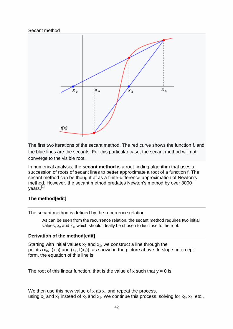
The first two iterations of the secant method. The red curve shows the function f, and

the blue lines are the secants. For this particular case, the secant method will not

converge to the visible root.

In numerical analysis, the secant method is a root-finding algorithm that uses a succession of roots of secant lines to better approximate a root of a function f. The secant method can be thought of as a finite-difference approximation of Newton's method. However, the secant method predates Newton's method by over 3000 years.[1]

The method[edit]

The secant method is defined by the recurrence relation

As can be seen from the recurrence relation, the secant method requires two initial

values, x0 and x1, which should ideally be chosen to lie close to the root.

Derivation of the method[edit]

Starting with initial values x0 and x1, we construct a line through the points (x0, f(x0)) and (x1, f(x1)), as shown in the picture above. In slope–intercept form, the equation of this line is

The root of this linear function, that is the value of x such that y = 0 is

We then use this new value of x as x2 and repeat the process, using x1 and x2 instead of x0 and x1. We continue this process, solving for x3, x4, etc.,

43

until we reach a sufficiently high level of precision (a sufficiently small difference between xn and xn−1):

Convergence[edit]

The iterates {\displaystyle x_{n}} of the secant method converge to a root

of {\displaystyle f} if the initial values {\displaystyle x_{0}} and {\displaystyle x_{1}} are

sufficiently close to the root. The order of convergence is υ, where

{\displaystyle \varphi ={\frac {1+{\sqrt {5}}}{2}}\approx 1.618}is the golden ratio. In

particular, the convergence is superlinear, but not quite quadratic.

This result only holds under some technical conditions, namely that {\displaystyle

f} be twice continuously differentiable and the root in question be simple (i.e., with

multiplicity 1).

If the initial values are not close enough to the root, then there is no guarantee that

the secant method converges. There is no general definition of "close enough", but

the criterion has to do with how "wiggly" the function is on the interval {\displaystyle

[x_{0},x_{1}]}. For example, if {\displaystyle f} is differentiable on that interval and

there is a point where {\displaystyle f'=0} on the interval, then the algorithm may not

converge.

Comparison with other root-finding methods[edit]

The secant method does not require that the root remain bracketed, like the bisection method does, and hence it does not always converge. The false position method (or regula falsi) uses the same formula as the secant method.

However, it does not apply the formula on and , like the secant method, but on and on the last iterate such that and have a different sign. This means that the false position method always converges.

The recurrence formula of the secant method can be derived from the formula for Newton's method

by using the finite-difference approximation

The secant method can be interpreted as a method in which the derivative is replaced by an approximation and is thus a quasi-Newton method.

If we compare Newton's method with the secant method, we see that Newton's method converges faster (order 2 against υ ≈ 1.6). However, Newton's method requires the evaluation of both and its derivative at every step, while the secant method only requires the evaluation of . Therefore, the secant method may

occasionally be faster in practice. For instance, if we assume that evaluating takes as much time as evaluating its derivative and we neglect all other costs, we can do two steps of the secant method (decreasing the logarithm of the error by a

44

factor υ2 ≈ 2.6) for the same cost as one step of Newton's method (decreasing the logarithm of the error by a factor 2), so the secant method is faster. If, however, we consider parallel processing for the evaluation of the derivative, Newton's method proves its worth, being faster in time, though still spending more steps.

Generalizations[edit]

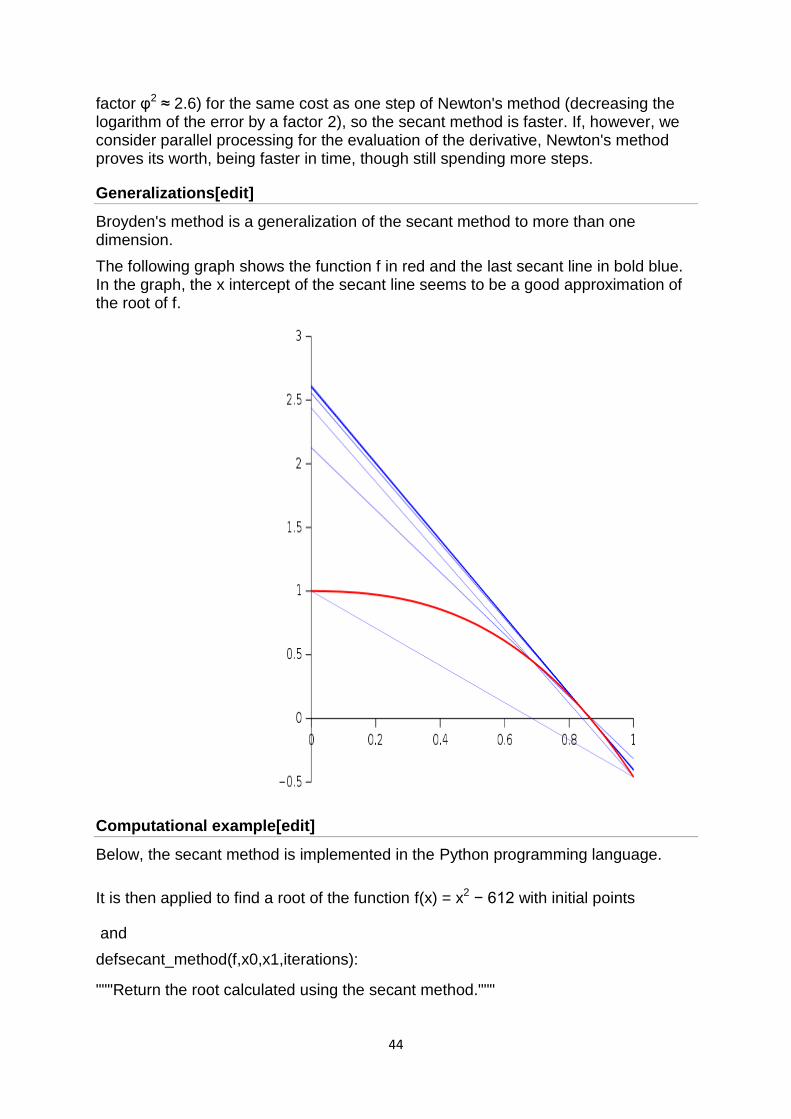
Broyden's method is a generalization of the secant method to more than one dimension.

The following graph shows the function f in red and the last secant line in bold blue. In the graph, the x intercept of the secant line seems to be a good approximation of the root of f.

Computational example[edit]

Below, the secant method is implemented in the Python programming language.

It is then applied to find a root of the function f(x) = x2 − 612 with initial points

and

defsecant_method(f,x0,x1,iterations):

"""Return the root calculated using the secant method."""

45

foriinrange(iterations):

x2=x1-f(x1)*(x1-x0)/float(f(x1)-f(x0))

x0,x1=x1,x2

returnx2

deff_example(x):

returnx**2-612

root=secant_method(f_example,10,30,5)

print("Root: {}".format(root))# Root: 24.738633748750722

Rate of convergence of iterative methods.

The term ―iterative method‖ refers to a wide range of techniques that use successive approximations to obtain more accurate solutions to a linear system at each step… In numerical analysis it attempts to solve a problem by finding successive approximations to the solution starting from an initial guess. This approach is in contrast to direct methods which attempt to solve the problem by a finite sequence of operations, and, in the absence of rounding errors, would deliver an exact solution Iterative methods are usually the only choice for non linear equations. However, iterative methods are often useful even for linear problems involving a large number of variables (sometimes of the order of millions), where direct methods would be prohibitively expensive (and in some cases impossible) even with the best available computing power.

Get Help With Your Essay

If you need assistance with writing your essay, our professional essay writing service is here to help!

Find out more

Stationary methods are older, simpler to understand and implement, but usually not as effective Stationary iterative method are the iterative methods that performs in each iteration the same operations on the current iteration vectors.Stationary iterative methods solve a linear system with an operator approximating the original one; and based on a measurement of the error in the result, form a ―correction equation‖ for which this process is repeated. While these methods are simple to derive, implement, and analyze, convergence is only guaranteed for a limited class of matrices. Examples of stationary iterative methods are the Jacobi method,gauss seidel method and the successive overrelaxation method.

46

The Nonstationary methods are based on the idea of sequences of orthogonal vectors Nonstationary methods are a relatively recent development; their analysis is usually harder to understand, but they can be highly effective These are the Iterative method that has iteration-dependent coefficients.It include Dense matrix: Matrix for which the number of zero elements is too small to warrant specialized algorithms. Sparse matrix: Matrix for which the number of zero elements is large enough that algorithms avoiding operations on zero elements pay off. Matrices derived from partial differential equations typically have a number of nonzero elements that is proportional to the matrix size, while the total number of matrix elements is the square of the matrix size.

The rate at which an iterative method converges depends greatly on the spectrum of the coefficient matrix. Hence, iterative methods usually involve a second matrix that transforms the coefficient matrix into one with a more favorable spectrum. The transformation matrix is called a preconditioner. A good preconditioner improves the convergence of the iterative method, sufficiently to overcome the extra cost of constructing and applying the preconditioner. Indeed, without a preconditioner the iterative method may even fail to converge.

Rate of Convergence

In numerical analysis, the speed at which a convergent sequence approaches its limit is called the rate of convergence. Although strictly speaking, a limit does not give information about any finite first part of the sequence, this concept is of practical importance if we deal with a sequence of successive approximations for an iterative method as then typically fewer iterations are needed to yield a useful approximation if the rate of convergence is higher. This may even make the difference between needing ten or a million iterations.Similar concepts are used for discretization methods. The solution of the discretized problem converges to the solution of the continuous problem as the grid size goes to zero, and the speed of convergence is one of the factors of the efficiency of the method. However, the terminology in this case is different from the terminology for iterative methods.

The rate of convergence of an iterative method is represented by mu (μ) and is defined as such:

Suppose the sequence{xn} (generated by an iterative method to find an approximation to a fixed point) converges to a point x, then

limn->[infinity] = |xn+1-x|/|xn-x|[alpha]=μ, where μâ‰≦0 and α(alpha)=order of convergence.

In cases where α=2 or 3 the sequence is said to have quadratic and cubic convergence respectively. However in linear cases i.e. when α=1, for the sequence to converge μ must be in the interval (0,1). The theory behind this is that for En+1≤μEn to converge the absolute errors must decrease with each approximation, and to guarantee this, we have to set 0<μ<1.

In cases where α=1 and μ=1 and you know it converges (since μ=1 does not tell us if it converges or diverges) the sequence {xn} is said to converge sublinearly i.e.

47

the order of convergence is less than one. If μ>1 then the sequence diverges. If μ=0 then it is said to converge superlinearly i.e. it‘s order of convergence is higher than 1, in these cases you change α to a higher value to find what the order of convergence is. In cases where μ is negative, the iteration diverges.

Stationary iterative methods

Stationary iterative methods are methods for solving a linear system of equations. Ax=B. where is a given matrix and is a given vector. Stationary iterative methods can be expressed in the simple form

where neither nor depends upon the iteration count . The four main stationary methods are the Jacobi Method,Gauss seidel method, successive overrelaxation method (SOR), and symmetric successive overrelaxation method (SSOR).

1.Jacobi method:- The Jacobi method is based on solving for every variable locally with respect to the other variables; one iteration of the method corresponds to solving for every variable once. The resulting method is easy to understand and implement, but convergence is slow. The Jacobi method is a method of solving a matrix equation on a matrix that has no zeros along its main diagonal . Each diagonal element is solved for, and an approximate value plugged in. The process is then iterated until it converges. This algorithm is a stripped-down version of the Jacobi transformation method of matrix diagnalization.

The Jacobi method is easily derived by examining each of the equations in the linear system of equations in isolation. If, in the th equation

solve for the value of while assuming the other entries of remain fixed. This gives

which is the Jacobi method.

In this method, the order in which the equations are examined is irrelevant, since the Jacobi method treats them independently. The definition of the Jacobi method can be expressed with matrices as

where the matrices , , and represent the diagnol, strictly lower triangular, and strictly upper triangular parts of , respectively

Convergence:- The standard convergence condition (for any iterative method) is when the spectral radius of the iteration matrix

ϕ(D ∑ 1R) < 1.

D is diagonal component,R is the remainder.

The method is guaranteed to converge if the matrix A is strictly or irreducibly diagonally dominant. Strict row diagonal dominance means that for each row, the absolute value of the diagonal term is greater than the sum of absolute values of other terms:

48

The Jacobi method sometimes converges even if these conditions are not satisfied.

2. Gauss-Seidel method:- The Gauss-Seidel method is like the Jacobi method, except that it uses updated values as soon as they are available. In general, if the Jacobi method converges, the Gauss-Seidel method will converge faster than the Jacobi method, though still relatively slowly. The Gauss-Seidel method is a technique for solving the equations of the linear system of equations one at a time in sequence, and uses previously computed results as soon as they are available,

There are two important characteristics of the Gauss-Seidel method should be noted. Firstly, the computations appear to be serial. Since each component of the new iterate depends upon all previously computed components, the updates cannot be done simultaneously as in the Jacobi method. Secondly, the new iterate depends upon the order in which the equations are examined. If this ordering is changed, the components of the new iterates (and not just their order) will also change. In terms of matrices, the definition of the Gauss-Seidel method can be expressed as

where the matrices , , and represent the diagonal, strictly lower triangular, and strictly upper triangular parts of A, respectively.

The Gauss-Seidel method is applicable to strictly diagonally dominant, or symmetric positive definite matrices A.

Convergence:-

Given a square system of n linear equations with unknown x:

The convergence properties of the Gauss-Seidel method are dependent on the matrix A. Namely, the procedure is known to converge if either:

A is symmetric positive definite, or

A is strictly or irreducibly diagonally dominant.

The Gauss-Seidel method sometimes converges even if these conditions are not satisfied.

3.Successive Overrelaxation method:-

The successive overrelaxation method (SOR) is a method of solving a linear system of equations derived by extrapolating the gauss-seidel method. This extrapolation takes the form of a weighted average between the previous iterate and the computed Gauss-Seidel iterate successively for each component,

where denotes a Gauss-Seidel iterate and is the extrapolation factor. The idea is to choose a value for that will accelerate the rate of convergence of the iterates to the solution.

In matrix terms, the SOR algorithm can be written as

49

where the matrices , , and represent the diagonal, strictly lower-triangular, and strictly upper-triangular parts of , respectively.

If , the SOR method simplifies to the gauss-seidel method. A theorem due to Kahan shows that SOR fails to converge if is outside the interval .

In general, it is not possible to compute in advance the value of that will maximize the rate of convergence of SOR. Frequently, some heuristic estimate is used, such as where is the mesh spacing of the discretization of the underlying physical domain.

Convergence:-

Successive Overrelaxation method may converge faster than Gauss-Seidel by an order of magnitude. We seek the solution to set of linear equations

In matrix terms, the successive over-relaxation (SOR) iteration can be expressed as

where , , and represent the diagonal, lower triangular, and upper triangular parts of the coefficient matrix , is the iteration count, and is a relaxation factor. This matrix expression is not usually used to program the method, and an element-based expression is used

Find out how UKEssays.com can help you!

Our academic experts are ready and waiting to assist with any writing project you may have. From simple essay plans, through to full dissertations, you can guarantee we have a service perfectly matched to your needs.

View our services

Note that for that the iteration reduces to the gauss-seidel iteration. As with the Gauss seidel method, the computation may be done in place, and the iteration is continued until the changes made by an iteration are below some tolerance.

The choice of relaxation factor is not necessarily easy, and depends upon the properties of the coefficient matrix. For symmetric, positive definite matrices it can be proven that will lead to convergence, but we are generally interested in faster convergence rather than just convergence.

4.Symmetric Successive overrelaxation:- Symmetric Successive Overrelaxation (SSOR) has no advantage over SOR as a stand-alone iterative method; however, it is useful as a preconditioner for nonstationary methods The symmetric successive overrelaxation (SSOR) method combines two successive overrelaxation method (SOR) sweeps together in such a way that the resulting iteration matrix is similar to a symmetric matrix it the case that the coefficient matrix of the linear system is symmetric. The SSOR is a forward SOR sweep followed by a backward SOR sweep in which the unknowns are updated in the reverse order. The similarity of the SSOR iteration matrix to a symmetric matrix permits the application of SSOR as a preconditioner for other iterative schemes for symmetric matrices. This is the

50

primary motivation for SSOR, since the convergence rate is usually slower than the convergence rate for SOR with optimal ..

Non-Stationary Iterative Methods:-

1.Conjugate Gradient method:- The conjugate gradient method derives its name from the fact that it generates a sequence of conjugate (or orthogonal) vectors. These vectors are the residuals of the iterates. They are also the gradients of a quadratic functional, the minimization of which is equivalent to solving the linear system. CG is an extremely effective method when the coefficient matrix is symmetric positive definite, since storage for only a limited number of vectors is required. Suppose we want to solve the following system of linear equations

Ax = b

where the n-by-n matrix A is symmetric (i.e., AT = A), positive definite (i.e., xTAx > 0 for all non-zero vectors x in Rn), and real.

We denote the unique solution of this system by x*.

We say that two non-zero vectors u and v are conjugate (with respect to A) if

Since A is symmetric and positive definite, the left-hand side defines an inner product

So, two vectors are conjugate if they are orthogonal with respect to this inner product. Being conjugate is a symmetric relation: if u is conjugate to v, then v is conjugate to u.

Convergence:- Accurate predictions of the convergence of iterative methods are difficult to make, but useful bounds can often be obtained. For the Conjugate Gradient method, the error can be bounded in terms of the spectral condition number of the matrix . ( if and are the largest and smallest eigenvalues of a symmetric positive definite matrix , then the spectral condition number of is . If is the exact solution of the linear system , with symmetric positive definite matrix , then for CG with symmetric positive definite preconditioner , it can be shown that

where , and . From this relation we see that the number of iterations to reach a relative reduction of in the error is proportional to .

In some cases, practical application of the above error bound is straightforward. For example, elliptic second order partial differential equations typically give rise to coefficient matrices with (where is the discretization mesh width), independent of the order of the finite elements or differences used, and of the number of space dimensions of the problem . Thus, without preconditioning, we expect a number of iterations proportional to for the Conjugate Gradient method.

Other results concerning the behavior of the Conjugate Gradient algorithm have been obtained. If the extremal eigenvalues of the matrix are well separated, then one often observes so-called; that is, convergence at a rate that increases per iteration. This phenomenon is explained by the fact that CG tends to eliminate

51

components of the error in the direction of eigenvectors associated with extremal eigenvalues first. After these have been eliminated, the method proceeds as if these eigenvalues did not exist in the given system, i.e., the convergence rate depends on a reduced system with a smaller condition number. The effectiveness of the preconditioner in reducing the condition number and in separating extremal eigenvalues can be deduced by studying the approximated eigenvalues of the related Lanczos process.

2. Biconjugate Gradient Method-The Biconjugate Gradient method generates two CG-like sequences of vectors, one based on a system with the original coefficient matrix , and one on . Instead of orthogonalizing each sequence, they are made mutually orthogonal, or ―bi-orthogonal‖. This method, like CG, uses limited storage. It is useful when the matrix is nonsymmetric and nonsingular; however, convergence may be irregular, and there is a possibility that the method will break down. BiCG requires a multiplication with the coefficient matrix and with its transpose at each iteration.

Convergence:- Few theoretical results are known about the convergence of BiCG. For symmetric positive definite systems the method delivers the same results as CG, but at twice the cost per iteration. For nonsymmetric matrices it has been shown that in phases of the process where there is significant reduction of the norm of the residual, the method is more or less comparable to full GMRES (in terms of numbers of iterations). In practice this is often confirmed, but it is also observed that the convergence behavior may be quite irregular , and the method may even break down . The breakdown situation due to the possible event that can be circumvented by so-called look-ahead strategies. This leads to complicated codes. The other breakdown situation, , occurs when the -decomposition fails, and can be repaired by using another decomposition.

Sometimes, breakdown or near-breakdown situations can be satisfactorily avoided by a restart at the iteration step immediately before the breakdown step. Another possibility is to switch to a more robust method, like GMRES.

3. Conjugate Gradient Squared (CGS ).

The Conjugate Gradient Squared method is a variant of BiCG that applies the updating operations for the -sequence and the -sequences both to the same vectors. Ideally, this would double the convergence rate, but in practice convergence may be much more irregular than for BiCG, which may sometimes lead to unreliable results. A practical advantage is that the method does not need the multiplications with the transpose of the coefficient matrix.

often one observes a speed of convergence for CGS that is about twice as fast as for BiCG, which is in agreement with the observation that the same ―contraction‖ operator is applied twice. However, there is no reason that the ―contraction‖ operator, even if it really reduces the initial residual , should also reduce the once reduced vector . This is evidenced by the often highly irregular convergence behavior of CGS . One should be aware of the fact that local corrections to the current solution may be so large that cancelation effects occur. This may lead to a less accurate

52

solution than suggested by the updated residual. The method tends to diverge if the starting guess is close to the solution.

4 Biconjugate Gradient Stabilized (Bi-CGSTAB ).

The Biconjugate Gradient Stabilized method is a variant of BiCG, like CGS, but using different updates for the -sequence in order to obtain smoother convergence than CGS. Bi-CGSTAB often converges about as fast as CGS, sometimes faster and sometimes not. CGS can be viewed as a method in which the BiCG ―contraction‖ operator is applied twice. Bi-CGSTAB can be interpreted as the product of BiCG and repeatedly applied GMRES. At least locally, a residual vector is minimized , which leads to a considerably smoother convergence behavior. On the other hand, if the local GMRES step stagnates, then the Krylov subspace is not expanded, and Bi-CGSTAB will break down . This is a breakdown situation that can occur in addition to the other breakdown possibilities in the underlying BiCG algorithm. This type of breakdown may be avoided by combining BiCG with other methods, i.e., by selecting other values for One such alternative is Bi-CGSTAB2 ; more general approaches are suggested by Sleijpen and Fokkema.

5..Chebyshev Iteration.

The Chebyshev Iteration recursively determines polynomials with coefficients chosen to minimize the norm of the residual in a min-max sense. The coefficient matrix must be positive definite and knowledge of the extremal eigenvalues is required. This method has the advantage of requiring no inner products. Chebyshev Iteration is another method for solving nonsymmetric problems . Chebyshev Iteration avoids the computation of inner products as is necessary for the other nonstationary methods. For some distributed memory architectures these inner products are a bottleneck with respect to efficiency. The price one pays for avoiding inner products is that the method requires enough knowledge about the spectrum of the coefficient matrix that an ellipse enveloping the spectrum can be identified ; however this difficulty can be overcome via an adaptive construction developed by Manteuffel , and implemented by Ashby . Chebyshev iteration is suitable for any nonsymmetric linear system for which the enveloping ellipse does not include the origin.

Convergence:-

In the symmetric case (where and the preconditioner are both symmetric) for the Chebyshev Iteration we have the same upper bound as for the Conjugate Gradient method, provided and are computed from and (the extremal eigenvalues of the preconditioned matrix ).

There is a severe penalty for overestimating or underestimating the field of values. For example, if in the symmetric case is underestimated, then the method may diverge; if it is overestimated then the result may be very slow convergence. Similar statements can be made for the nonsymmetric case. This implies that one needs fairly accurate bounds on the spectrum of for the method to be effective (in comparison with CG or GMRES).

53

Acceleration of convergence

Many methods exist to increase the rate of convergence of a given sequence, i.e. to transform a given sequence into one converging faster to the same limit. Such techniques are in general known as ―series acceleration‖. The goal of the transformed sequence is to be much less ―expensive‖ to calculate than the original sequence. One example of series acceleration is Aitken‘s delta -squared process.

54

Unit-III Simultaneous Linear Equations

Solutions of system of Linear equations

A Linear Equation is an equation for a line.

A linear equation is not always in the form y = 3.5 − 0.5x,

It can also be like y = 0.5(7 − x)

Or like y + 0.5x = 3.5

Or like y + 0.5x − 3.5 = 0 and more.

(Note: those are all the same linear equation!)

A System of Linear Equations is when we have two or more linear equations working together.

Example: Here are two linear equations:

2x + y = 5

−x + y = 2

Together they are a system of linear equations.

Can you discover the values of x and y yourself? (Just have a go, play with them a bit.)

Let's try to build and solve a real world example:

Example: You versus Horse

55

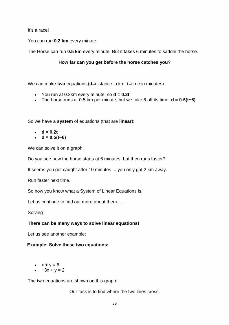
It's a race!

You can run 0.2 km every minute.

The Horse can run 0.5 km every minute. But it takes 6 minutes to saddle the horse.

How far can you get before the horse catches you?

We can make two equations (d=distance in km, t=time in minutes)

You run at 0.2km every minute, so d = 0.2t The horse runs at 0.5 km per minute, but we take 6 off its time: d = 0.5(t−6)

So we have a system of equations (that are linear):

d = 0.2t d = 0.5(t−6)

We can solve it on a graph:

Do you see how the horse starts at 6 minutes, but then runs faster?

It seems you get caught after 10 minutes ... you only got 2 km away.

Run faster next time.

So now you know what a System of Linear Equations is.

Let us continue to find out more about them ....

Solving

There can be many ways to solve linear equations!

Let us see another example:

Example: Solve these two equations:

x + y = 6 −3x + y = 2

The two equations are shown on this graph:

Our task is to find where the two lines cross.

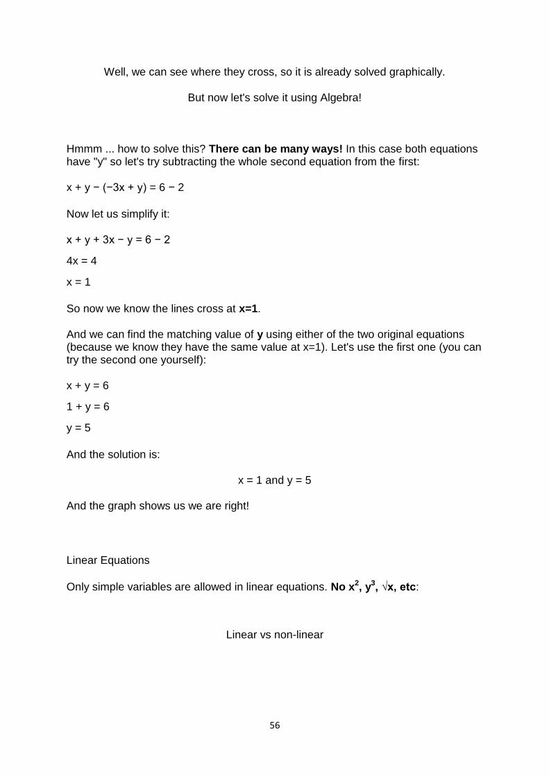
56

Well, we can see where they cross, so it is already solved graphically.

But now let's solve it using Algebra!

Hmmm ... how to solve this? There can be many ways! In this case both equations have "y" so let's try subtracting the whole second equation from the first:

x + y − (−3x + y) = 6 − 2

Now let us simplify it:

x + y + 3x − y = 6 − 2

4x = 4

x = 1

So now we know the lines cross at x=1.

And we can find the matching value of y using either of the two original equations (because we know they have the same value at x=1). Let's use the first one (you can try the second one yourself):

x + y = 6

1 + y = 6

y = 5

And the solution is:

x = 1 and y = 5

And the graph shows us we are right!

Linear Equations

Only simple variables are allowed in linear equations. No x2, y3, √x, etc:

Linear vs non-linear

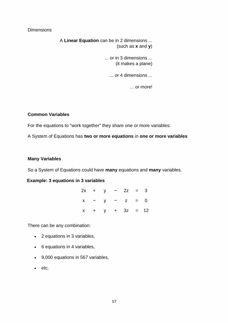
57

Dimensions

A Linear Equation can be in 2 dimensions ...

(such as x and y)

... or in 3 dimensions ...

(it makes a plane)

... or 4 dimensions ...

... or more!

Common Variables

For the equations to "work together" they share one or more variables:

A System of Equations has two or more equations in one or more variables

Many Variables

So a System of Equations could have many equations and many variables.

Example: 3 equations in 3 variables

2x + y − 2z = 3

x − y − z = 0

x + y + 3z = 12

There can be any combination:

2 equations in 3 variables,

6 equations in 4 variables,

9,000 equations in 567 variables,

etc.

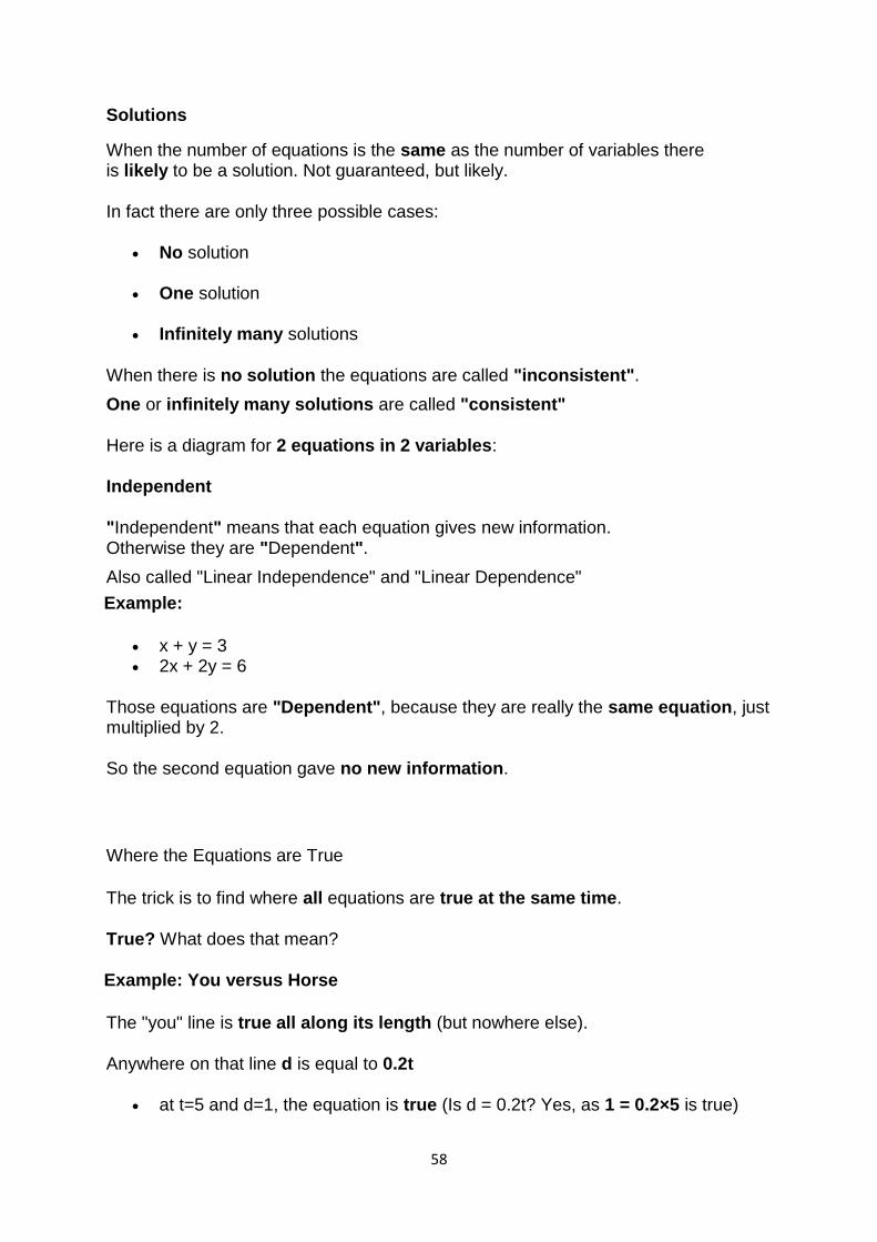
58

Solutions

When the number of equations is the same as the number of variables there is likely to be a solution. Not guaranteed, but likely.

In fact there are only three possible cases:

No solution

One solution

Infinitely many solutions

When there is no solution the equations are called "inconsistent".

One or infinitely many solutions are called "consistent"

Here is a diagram for 2 equations in 2 variables:

Independent

"Independent" means that each equation gives new information. Otherwise they are "Dependent".

Also called "Linear Independence" and "Linear Dependence"

Example:

x + y = 3 2x + 2y = 6

Those equations are "Dependent", because they are really the same equation, just multiplied by 2.

So the second equation gave no new information.

Where the Equations are True

The trick is to find where all equations are true at the same time.

True? What does that mean?

Example: You versus Horse

The "you" line is true all along its length (but nowhere else).

Anywhere on that line d is equal to 0.2t

at t=5 and d=1, the equation is true (Is d = 0.2t? Yes, as 1 = 0.2×5 is true)

59

at t=5 and d=3, the equation is not true (Is d = 0.2t? No, as 3 = 0.2×5 is not true)

Likewise the "horse" line is also true all along its length (but nowhere else).

But only at the point where they cross (at t=10, d=2) are they both true.

So they have to be true simultaneously ...

... that is why some people call them "Simultaneous Linear Equations"

Solve Using Algebra

It is common to use Algebra to solve them.

Here is the "Horse" example solved using Algebra:

Example: You versus Horse

The system of equations is:

d = 0.2t d = 0.5(t−6)

In this case it seems easiest to set them equal to each other:

d = 0.2t = 0.5(t−6)

Start with:0.2t = 0.5(t − 6)

Expand 0.5(t−6):0.2t = 0.5t − 3

Subtract 0.5t from both sides:−0.3t = −3

Divide both sides by −0.3:t = −3/−0.3 = 10 minutes

Now we know when you get caught!

Knowing t we can calculate d:d = 0.2t = 0.2×10 = 2 km

And our solution is:

t = 10 minutes and d = 2 km

60

Algebra vs Graphs

Why use Algebra when graphs are so easy? Because:

More than 2 variables can't be solved by a simple graph.

So Algebra comes to the rescue with two popular methods:

Solving By Substitution Solving By Elimination

We will see each one, with examples in 2 variables, and in 3 variables. Here goes ... Solving By Substitution

These are the steps:

Write one of the equations so it is in the style "variable = ..."

Replace (i.e. substitute) that variable in the other equation(s).

Solve the other equation(s)

(Repeat as necessary)

Here is an example with 2 equations in 2 variables:

Example:

3x + 2y = 19 x + y = 8

We can start with any equation and any variable.

Let's use the second equation and the variable "y" (it looks the simplest equation).

Write one of the equations so it is in the style "variable = ...":

We can subtract x from both sides of x + y = 8 to get y = 8 − x. Now our equations look like this:

3x + 2y = 19 y = 8 − x

Now replace "y" with "8 − x" in the other equation:

61

3x + 2(8 − x) = 19 y = 8 − x

Solve using the usual algebra methods:

Expand 2(8−x):

3x + 16 − 2x = 19 y = 8 − x

Then 3x−2x = x:

x + 16 = 19 y = 8 − x

And lastly 19−16=3

x = 3 y = 8 − x

Now we know what x is, we can put it in the y = 8 − x equation:

x = 3 y = 8 − 3 = 5

And the answer is:

x = 3 y = 5

Note: because there is a solution the equations are "consistent"

Check: why don't you check to see if x = 3 and y = 5 works in both equations?

Solving By Substitution: 3 equations in 3 variables

OK! Let's move to a longer example: 3 equations in 3 variables.

This is not hard to do... it just takes a long time!

Example:

x + z = 6 z − 3y = 7

62

2x + y + 3z = 15

We should line up the variables neatly, or we may lose track of what we are doing:

x + z = 6

− 3y + z = 7

2x + y + 3z = 15

WeI can start with any equation and any variable. Let's use the first equation and the variable "x".

Write one of the equations so it is in the style "variable = ...":

x = 6 − z

− 3y + z = 7

2x + y + 3z = 15

Now replace "x" with "6 − z" in the other equations:

(Luckily there is only one other equation with x in it)

x = 6 − z

− 3y + z = 7

2(6−z) + y + 3z = 15

Solve using the usual algebra methods:

2(6−z) + y + 3z = 15 simplifies to y + z = 3:

x = 6 − z

− 3y + z = 7

63

y + z = 3

Good. We have made some progress, but not there yet.

Now repeat the process, but just for the last 2 equations.

Write one of the equations so it is in the style "variable = ...":

Let's choose the last equation and the variable z:

x = 6 − z

− 3y + z = 7

z = 3 − y

Now replace "z" with "3 − y" in the other equation:

x = 6 − z

− 3y + 3 − y = 7

z = 3 − y

Solve using the usual algebra methods:

−3y + (3−y) = 7 simplifies to −4y = 4, or in other words y = −1

x = 6 − z

y = −1

z = 3 − y

Almost Done!

Knowing that y = −1 we can calculate that z = 3−y = 4:

x = 6 − z

64

y = −1

z = 4

And knowing that z = 4 we can calculate that x = 6−z = 2:

x = 2

y = −1

z = 4

And the answer is:

x = 2 y = −1 z = 4

Check: please check this yourself.

We can use this method for 4 or more equations and variables... just do the same steps again and again until it is solved.

Conclusion: Substitution works nicely, but does take a long time to do.

Solving By Elimination

Elimination can be faster ... but needs to be kept neat.

"Eliminate" means to remove: this method works by removing variables until there is just one left.

The idea is that we can safely:

multiply an equation by a constant (except zero), add (or subtract) an equation on to another equation

Like in these examples:

65

WHY can we add equations to each other?

Imagine two really simple equations:

x − 5 = 3 5 = 5

We can add the "5 = 5" to "x − 5 = 3":

x − 5 + 5 = 3 + 5 x = 8

Try that yourself but use 5 = 3+2 as the 2nd equation

It will still work just fine, because both sides are equal (that is what the = is for!)

We can also swap equations around, so the 1st could become the 2nd, etc, if that helps.

OK, time for a full example. Let's use the 2 equations in 2 variables example from before:

Example:

3x + 2y = 19 x + y = 8

Very important to keep things neat:

3x + 2y = 19

x + y = 8

Now ... our aim is to eliminate a variable from an equation.

First we see there is a "2y" and a "y", so let's work on that.

Multiply the second equation by 2:

3x + 2y = 19

2x + 2y = 16

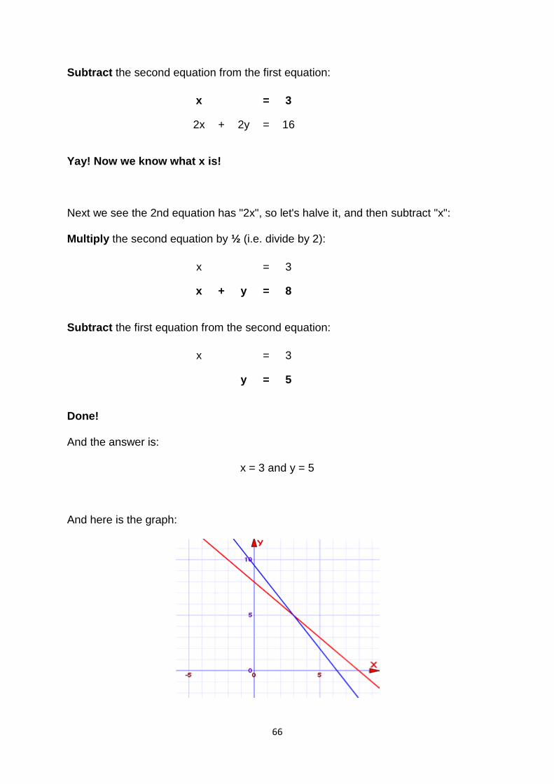
66

Subtract the second equation from the first equation:

x = 3

2x + 2y = 16

Yay! Now we know what x is!

Next we see the 2nd equation has "2x", so let's halve it, and then subtract "x":

Multiply the second equation by ½ (i.e. divide by 2):

x = 3

x + y = 8

Subtract the first equation from the second equation:

x = 3

y = 5

Done!

And the answer is:

x = 3 and y = 5

And here is the graph:

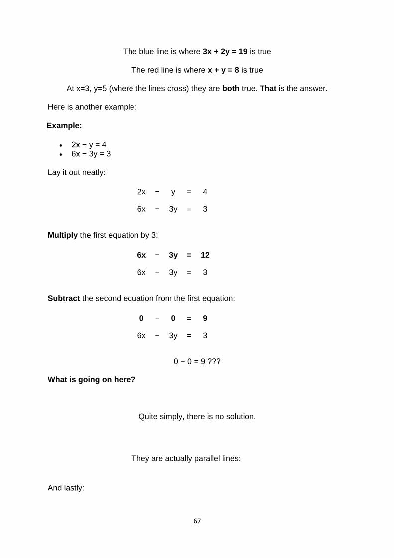
67

The blue line is where 3x + 2y = 19 is true

The red line is where x + y = 8 is true

At x=3, y=5 (where the lines cross) they are both true. That is the answer.

Here is another example:

Example:

2x − y = 4 6x − 3y = 3

Lay it out neatly:

2x − y = 4

6x − 3y = 3

Multiply the first equation by 3:

6x − 3y = 12

6x − 3y = 3

Subtract the second equation from the first equation:

0 − 0 = 9

6x − 3y = 3

0 − 0 = 9 ???

What is going on here?

Quite simply, there is no solution.

They are actually parallel lines:

And lastly:

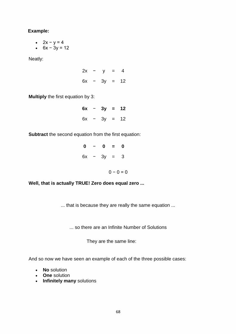
68

Example:

2x − y = 4 6x − 3y = 12

Neatly:

2x − y = 4

6x − 3y = 12

Multiply the first equation by 3:

6x − 3y = 12

6x − 3y = 12

Subtract the second equation from the first equation:

0 − 0 = 0

6x − 3y = 3

0 − 0 = 0

Well, that is actually TRUE! Zero does equal zero ...

... that is because they are really the same equation ...

... so there are an Infinite Number of Solutions

They are the same line:

And so now we have seen an example of each of the three possible cases:

No solution One solution Infinitely many solutions

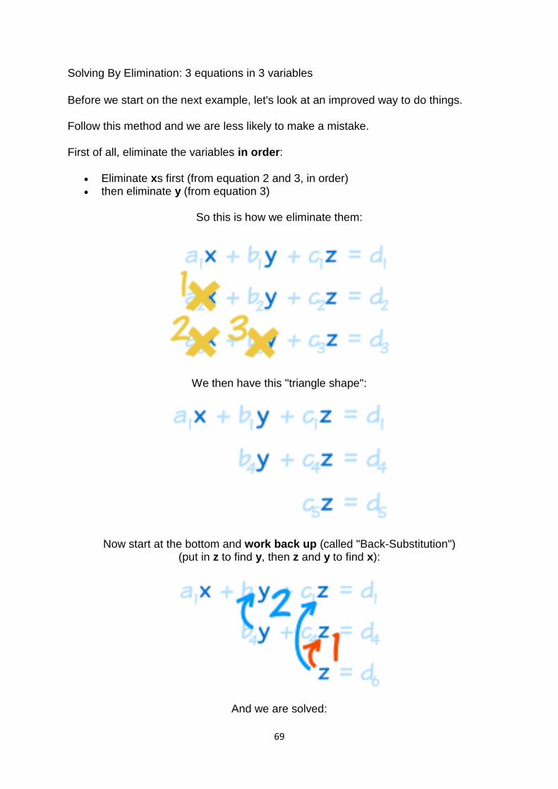
69

Solving By Elimination: 3 equations in 3 variables

Before we start on the next example, let's look at an improved way to do things.

Follow this method and we are less likely to make a mistake.

First of all, eliminate the variables in order:

Eliminate xs first (from equation 2 and 3, in order) then eliminate y (from equation 3)

So this is how we eliminate them:

We then have this "triangle shape":

Now start at the bottom and work back up (called "Back-Substitution") (put in z to find y, then z and y to find x):

And we are solved:

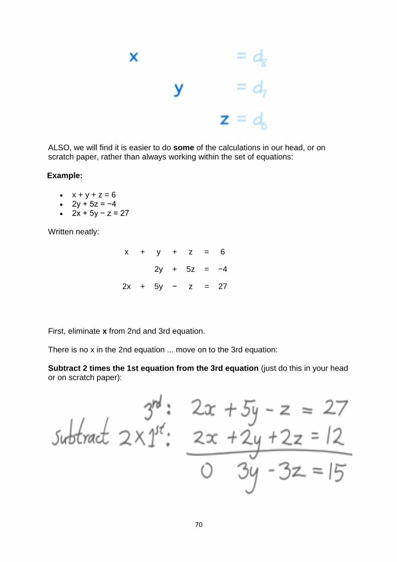
70

ALSO, we will find it is easier to do some of the calculations in our head, or on scratch paper, rather than always working within the set of equations:

Example:

x + y + z = 6 2y + 5z = −4 2x + 5y − z = 27

Written neatly:

x + y + z = 6

2y + 5z = −4

2x + 5y − z = 27

First, eliminate x from 2nd and 3rd equation.

There is no x in the 2nd equation ... move on to the 3rd equation:

Subtract 2 times the 1st equation from the 3rd equation (just do this in your head or on scratch paper):

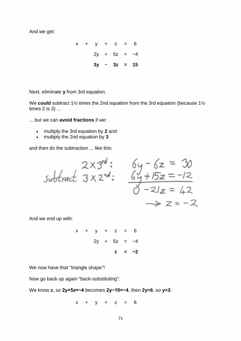
71

And we get:

x + y + z = 6

2y + 5z = −4

3y − 3z = 15

Next, eliminate y from 3rd equation.

We could subtract 1½ times the 2nd equation from the 3rd equation (because 1½ times 2 is 3) ...

... but we can avoid fractions if we:

multiply the 3rd equation by 2 and multiply the 2nd equation by 3

and then do the subtraction ... like this:

And we end up with:

x + y + z = 6

2y + 5z = −4

z = −2

We now have that "triangle shape"!

Now go back up again "back-substituting":

We know z, so 2y+5z=−4 becomes 2y−10=−4, then 2y=6, so y=3:

x + y + z = 6

72

y = 3

z = −2

Then x+y+z=6 becomes x+3−2=6, so x=6−3+2=5

x = 5

y = 3

z = −2

And the answer is:

x = 5 y = 3

z = −2

Check: please check for yourself.

General Advice

Once you get used to the Elimination Method it becomes easier than Substitution, because you just follow the steps and the answers appear.

But sometimes Substitution can give a quicker result.

Substitution is often easier for small cases (like 2 equations, or sometimes 3 equations)

Elimination is easier for larger cases

And it always pays to look over the equations first, to see if there is an easy shortcut ... so experience helps.

Gaussian Elimination with Partial Pivoting

Terry D. Johnson 10.001 Fall 2000

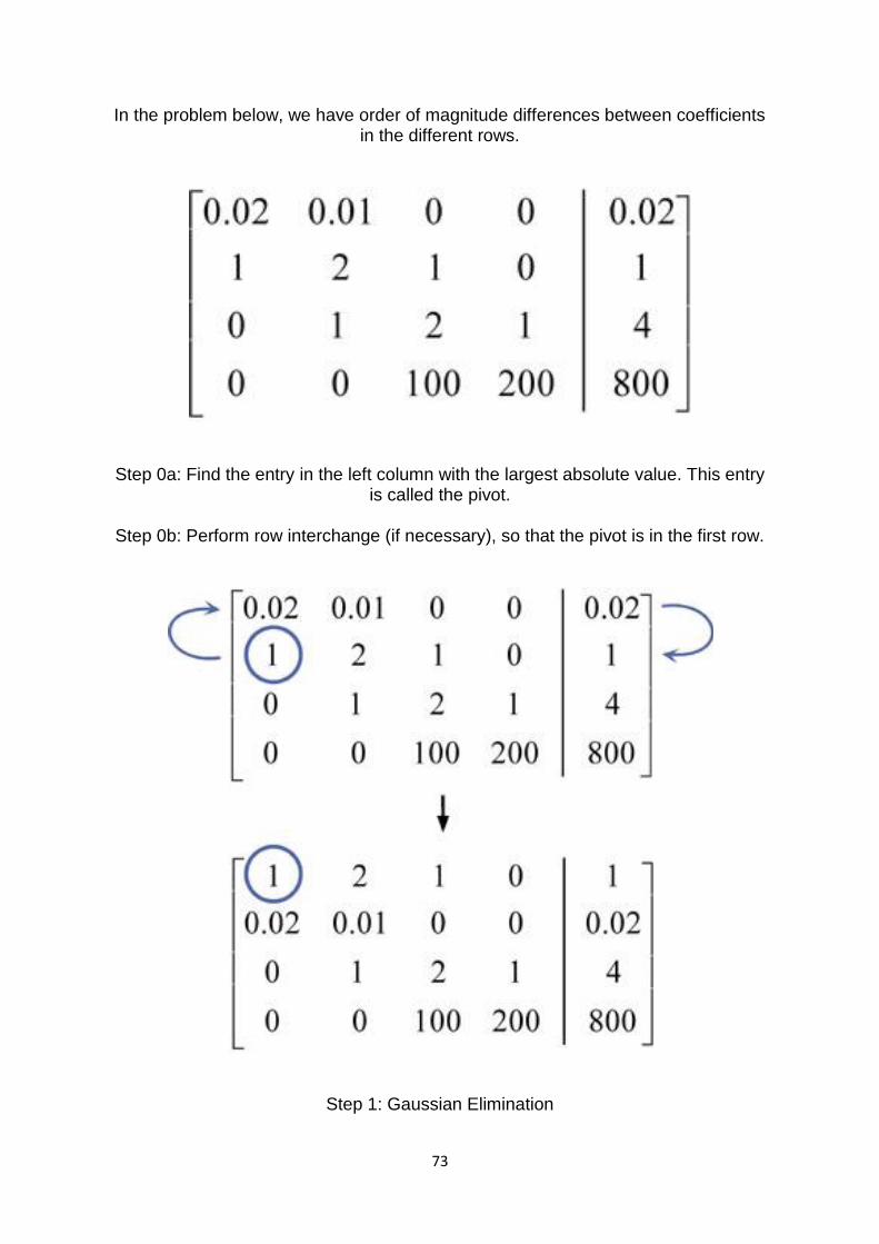
73

In the problem below, we have order of magnitude differences between coefficients in the different rows.

Step 0a: Find the entry in the left column with the largest absolute value. This entry is called the pivot.

Step 0b: Perform row interchange (if necessary), so that the pivot is in the first row.

Step 1: Gaussian Elimination

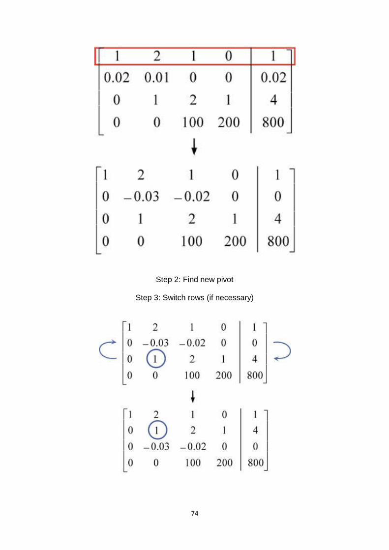
74

Step 2: Find new pivot

Step 3: Switch rows (if necessary)

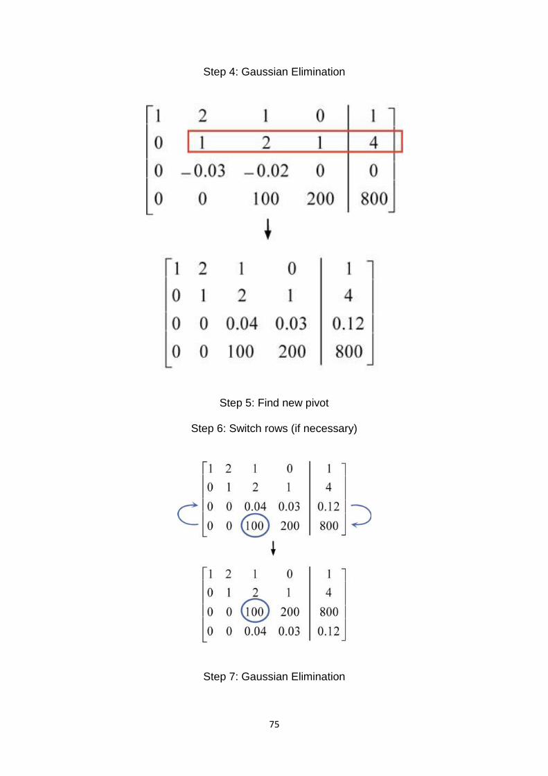
75

Step 4: Gaussian Elimination

Step 5: Find new pivot

Step 6: Switch rows (if necessary)

Step 7: Gaussian Elimination

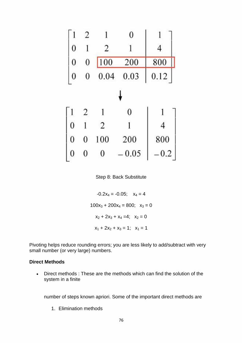
76

Step 8: Back Substitute

-0.2x4 = -0.05; x4 = 4

100x3 + 200x4 = 800; x3 = 0

x2 + 2x3 + x4 =4; x2 = 0

x1 + 2x2 + x3 = 1; x1 = 1

Pivoting helps reduce rounding errors; you are less likely to add/subtract with very small number (or very large) numbers.

Direct Methods

Direct methods : These are the methods which can find the solution of the system in a finite

number of steps known apriori. Some of the important direct methods are

1. Elimination methods

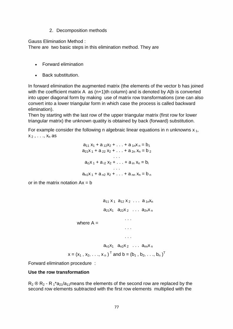
77

2. Decomposition methods

Gauss Elimination Method :

There are two basic steps in this elimination method. They are

Forward elimination

Back substitution.

In forward elimination the augmented matrix (the elements of the vector b has joined

with the coefficient matrix A as (n+1)th column) and is denoted by A|b is converted

into upper diagonal form by making use of matrix row transformations (one can also

convert into a lower triangular form in which case the process is called backward

elimination).

Then by starting with the last row of the upper triangular matrix (first row for lower

triangular matrix) the unknown quatity is obtained by back (forward) substitution.

For example consider the following n algebraic linear equations in n unknowns x 1,

x 2 , . . ., xn as

a11 x1 + a 12x2 + . . . + a 1nx n = b1

a21x 1 + a 22 x2 + . . . + a 2n xn = b 2

. . .

ai1x 1 + a i2 x2 + . . . + a in xn = bi

. . .

an1x 1 + a n2 x2 + . . . + a nn xn = b n

or in the matrix notation Ax = b

where A =

a11 x 1 a12 x 2 . . . a 1nxn

a21x1 a22x 2 . . . a2nx n

. . .

. . .

. . .

an1x1 an2x 2 . . . annx n

x = (x1 , x2, . . ., x n ) T and b = (b1 , b2, . . ., bn )

T

Forward elimination procedure :

Use the row transformation

R2 ® R2 - R 1*a21/a11means the elements of the second row are replaced by the second row elements subtracted with the first row elements multiplied with the

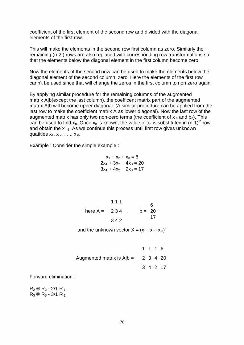
78

coefficient of the first element of the second row and divided with the diagonal elements of the first row.

This will make the elements in the second row first column as zero. Similarly the remaining (n-2 ) rows are also replaced with corresponding row transformations so that the elements below the diagonal element in the first column become zero.

Now the elements of the second now can be used to make the elements below the diagonal element of the second column, zero. Here the elements of the first row cann't be used since that will change the zeros in the first column to non zero again.

By applying similar procedure for the remaining columns of the augmented matrix A|b(except the last column), the coefficent matrix part of the augmented matrix A|b will become upper diagonal. (A similar procedure can be applied from the last row to make the coefficient matrix A as lower diagonal). Now the last row of the augmented matrix has only two non-zero terms (the coefficient of x n and bn). This can be used to find xn. Once xn is known, the value of xn is substituted in (n-1)th row and obtain the xn-1. As we continue this process until first row gives unknown quatities x1, x 2, . . ., x n.

Example : Consider the simple example :

x1 + x2 + x3 = 6

2x1 + 3x2 + 4x3 = 20

3x1 + 4x2 + 2x3 = 17

here A =

1 1 1

,

b =

6

20

17

2 3 4

3 4 2

and the unknown vector X = (x1 , x 2, x 3)T

Augmented matrix is A|b =

1 1 1 6

2 3 4 20

3 4 2 17

Forward elimination :

R2 ® R2 - 2/1 R 1 R3 ® R3 - 3/1 R 1

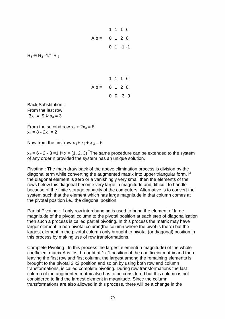
79

A|b =

1 1 1 6

0 1 2 8

0 1 -1 -1

R3 ® R3 -1/1 R 2

A|b =

1 1 1 6

0 1 2 8

0 0 -3 -9

Back Substitution :

From the last row

-3x3 = -9 Þ x3 = 3

From the second row x2 + 2x3 = 8 x2 = 8 - 2x3 = 2

Now from the first row x 1+ x2 + x 3 = 6

x1 = 6 - 2 - 3 =1 Þ x = (1, 2, 3) TThe same procedure can be extended to the system of any order n provided the system has an unique solution.

Pivoting : The main draw back of the above elimination process is division by the diagonal term while converting the augmented matrix into upper triangular form. If the diagonal element is zero or a vanishingly very small then the elements of the rows below this diagonal become very large in magnitude and difficult to handle because of the finite storage capacity of the computers. Alternative is to convert the system such that the element which has large magnitude in that column comes at the pivotal position i.e., the diagonal position.

Partial Pivoting : If only row interchanging is used to bring the element of large magnitude of the pivotal column to the pivotal position at each step of diagonalization then such a process is called partial pivoting. In this process the matrix may have larger element in non-pivotal column(the column where the pivot is there) but the largest element in the pivotal column only brought to pivotal (or diagonal) position in this process by making use of row transformations.

Complete Pivoting : In this process the largest element(in magnitude) of the whole coefficient matrix A is first brought at 1x 1 position of the coefficeint matrix and then leaving the first row and first column, the largest among the remaining elements is brought to the pivotal 2 x2 position and so on by using both row and column transformations, is called complete pivoting. During row transformations the last column of the augmented matrix also has to be considered but this column is not considered to find the largest element in magnitude. Since the column transformations are also allowed in this process, there will be a change in the

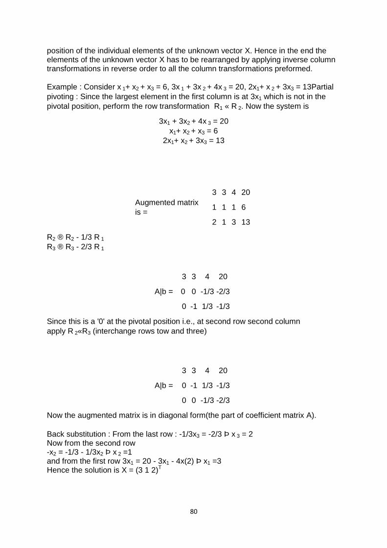
80

position of the individual elements of the unknown vector X. Hence in the end the elements of the unknown vector X has to be rearranged by applying inverse column transformations in reverse order to all the column transformations preformed.

Example : Consider x 1+ x2 + x3 = 6, 3x 1 + 3x 2 + 4x 3 = 20, 2x1+ x 2 + 3x3 = 13Partial

pivoting : Since the largest element in the first column is at 3x1 which is not in the

pivotal position, perform the row transformation R1 « R 2. Now the system is

3x1 + 3x2 + 4x 3 = 20

x1+ x2 + x3 = 6

2x1+ x2 + 3x3 = 13

Augmented matrix

is =

3 3 4 20

1 1 1 6

2 1 3 13

R2 ® R2 - 1/3 R 1

R3 ® R3 - 2/3 R 1

A|b =

3 3 4 20

0 0 -1/3 -2/3

0 -1 1/3 -1/3

Since this is a '0' at the pivotal position i.e., at second row second column

apply R 2«R3 (interchange rows tow and three)

A|b =

3 3 4 20

0 -1 1/3 -1/3

0 0 -1/3 -2/3

Now the augmented matrix is in diagonal form(the part of coefficient matrix A).

Back substitution : From the last row : -1/3x3 = -2/3 Þ x 3 = 2 Now from the second row -x2 = -1/3 - 1/3x2 Þ x 2 =1 and from the first row 3x1 = 20 - 3x1 - 4x(2) Þ x1 =3 Hence the solution is X = (3 1 2)T

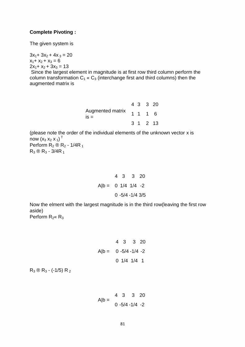
81

Complete Pivoting :

The given system is

3x1+ 3x2 + 4x 3 = 20 x1+ x2 + x3 = 6 2x1+ x2 + 3x3 = 13 Since the largest element in magnitude is at first row third column perform the column transformation C1 « C3 (interchange first and third columns) then the augmented matrix is

Augmented matrix

is =

4 3 3 20

1 1 1 6

3 1 2 13

(please note the order of the individual elements of the unknown vector x is

now (x3 x2 x 1) T

Perform R2 ® R2 - 1/4R 1

R3 ® R3 - 3/4R 1

A|b =

4 3 3 20

0 1/4 1/4 -2

0 -5/4 -1/4 3/5

Now the elment with the largest magnitude is in the third row(leaving the first row

aside)

Perform R2« R3

A|b =

4 3 3 20

0 -5/4 -1/4 -2

0 1/4 1/4 1

R3 ® R3 - (-1/5) R 2

A|b = 4 3 3 20

0 -5/4 -1/4 -2

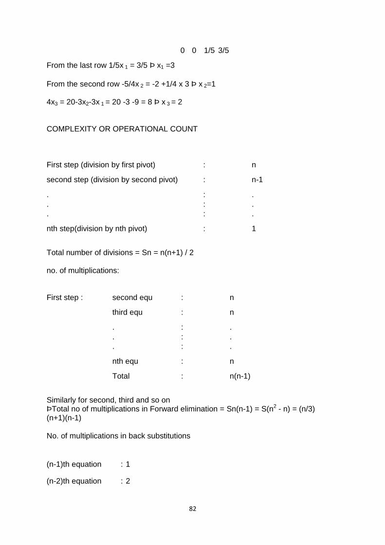
82

0 0 1/5 3/5

From the last row 1/5x 1 = 3/5 Þ x1 =3

From the second row -5/4x 2 = -2 +1/4 x 3 Þ x 2=1

4x3 = 20-3x2-3x 1 = 20 -3 -9 = 8 Þ x 3 = 2

COMPLEXITY OR OPERATIONAL COUNT

First step (division by first pivot) : n

second step (division by second pivot) : n-1

.

.

.

:

:

:

.

.

.

nth step(division by nth pivot) : 1

Total number of divisions = Sn = n(n+1) / 2

no. of multiplications:

First step : second equ : n

third equ : n

.

.

.

:

:

:

.

.

.

nth equ : n

Total : n(n-1)

Similarly for second, third and so on ÞTotal no of multiplications in Forward elimination = Sn(n-1) = S(n2 - n) = (n/3) (n+1)(n-1)

No. of multiplications in back substitutions

(n-1)th equation : 1

(n-2)th equation : 2

83

.

.

:

:

:

.

.

.

first equation : n-1

ÞTotal no of multiplications in back substitution = S(n-1) = (n/2)(n-1)

Total multiplications = (n/3)(n+1)(n-1) + (n/2)(n-1) = (n/6) (n-1)(2n+5)

Operational count = Total no of divisions and multiplications

= (n/2)(n+1) + (n/6)(n-1)(2n+5) = (n/3)(n2 +3n -1)

for very large 'n' the operational count is @ n3/3 or the complexity of the Gauss elimination is O(n3/3)

No. of additions and subtractions = (n/6)(n-1)(2n+5).

Similarly operational count for cholesky method is (1/6)(n3+9n2+2n).

Ill Conditioned Systems :

During computation it is not possible to store the numbers exactly in the computer but prone to some round off errors. If dA is the error in A and db is the error in b then

the equation Ax = b is actually solved for (A + dA) = b + db. (or)

|| - x|| < ||(A + dA)-1 - A-1|| ||b|| + ||(A + dA)-1|| ||db||

where ||.|| is any matrix norm

This gives

|| - x|| < (||A-1dA|| ||db||) (||A-1|| / (1 - ||A-1dA||))

|| - x|| < [ ||db|| / ||b|| + ||dA|| / ||dA|| ] ( k(A) / (1 - ||A-1dA||)))

where k(A) = ||A-1|| ||A-1|| is called the condition number of the matrix A. If k(A) is small (close to one) small change in A and b leads to small changes in x where as for large values of k(A) a small change in A or b (or both) leads to large changes in x. The systems for which k(A) is large are called ill conditioned systems.

Example : consider 2.1x +1.8y = 2.1 and 6.2x + 5.3y = 6.2

eigen value of A are 74.18 and l2 = 0.000012 if we use || ||2 for the norm then k(A) = Ö(l1/l2) = 2472.73 That is the given system is ill-conditioned.

84

Ill Conditioned system of equations

In this segment we'll talk about how to differentiate between ill-conditioned and well-

conditioned systems of equations. So let‘s suppose somebody gives you a system of

equations which is in the matrix form and turns out to be ax equals c. What A is the

coefficient matrix and c is the right hand side vector and of course x is our solution

vector or what we call as the unknown vector. So whenever we are solving or setting

up simultaneous linear equations we write them in the form of a times x equals c

where a is the coefficient matrix x is the solution vector and c is the right hand side

vector. What you would like to see is that if you wanted to find whether this

particular system of equations is well-conditioned or ill-conditioned is to say the

following: that hey if I make a small change in the elements of the a matrix then how

much change is it making in the solution vector? Or if I make a small change in my c

vector, then how much change does it make in my solution vector? Because you

would like that A if I make a small change in the coefficient matrix, you would like the

solution vector to change in a small amount or if you change the right hand side

vector you would like the solution vector to change in a small amount.

Because we are going to as we go through the process of setting up simultaneous

linear equations for real life problems those might be set up through a program

where we‘re going to have round-off errors in the calculation of the a matrix and the

calculation of the c matrix I suppose. We don‘t want such a round off errors or the

lack of our use of precision when we use only single precision rather than double

precision or quad precision to affect adversely what the solution vector is. If it does

we want to have a mechanism of knowing whether it is doing so.

So, let's look at some examples right here to see that if from a simple example if a

system of equations is well-conditioned and ill-conditioned. Let‘s suppose somebody

says is this particular system of equations 1 2 2 3.99 xy is equal to 4 7.999 well-

conditioned or ill-conditioned. We want to be able to make the difference between

saying that hey if someone gave me a system of equations like this one is it well-

conditioned or ill-conditioned. I can see that if I wanted to solve the set of equations it

does have a simple solution for example. What is the solution to this one? It's two

comma one. So x y is two comma one. So if we take x equal two and y equal one. In

fact, if you plug x equal to two and y equal to one in here you will get 4 and 7.999. So

that's itself a solution for that. And we want to see that whether if a small change in

the caution matrix is it going to result in a very different value x and y I'm going to

get. Or if I make a small change in my right hand side vector is it going to make a

make change in my x and y. And what I'm doing now here islet‘s suppose I make a

small change in my caution matrix. So What I'm doing is as follows. I'm taking 1.001

85

so I'm making a small change in the caution matrix. Changing by the thousands I get

3.998 so what I'm doing is that I‘m making a change of about a magnitude of point

zero zero one for all of these elements which are here in the caution matrix. And I'm

not changing the right hand side.

And I want to see that if hey does it make a big difference in my solution? And what I

find out is that hey that if I solve these two equations, two unknowns by hand or by

using Matlab or a new kind of calculator the answer that I should get is as follows

3.994 0.001388. And you can see that just by watching it or just by looking at it you

can see that this value of 2 has changed to almost 4. This value of 1 has

to changed to almost a value of 001. So very different with very small change being

made in the caution of the a matrix. So we can very well see that it is not a well-

conditioned system of equations. In order to complete the argument lets go and

change the right hand side a little bit. So let‘s suppose I have 1 2 2 3.999 here. And

what I do is I keep the caution matrix the same but I change the right hand side a

little bit. So let me make this to be again one thousandths off of a difference there

and 7.9998 here and one thousandths of a difference right here. And let‘s go and

see what I get for values of x and y. So I get x and y here and if I calculate the value

I get minus 3.999 and 4.00. So again you're finding out that from the original set of

equations you had right here where the solution was 2 and 1 I made a very small

change. I changed 4 to 4.001. I changed 7.999 to 7.998. Small change, small

relative change in the right hand side vector. But when I saw these two questions

these two unknowns by calculator, Matlab, whatever we find out that the solution

which I get is different. This was 2 now it is minus 3.999. This was 1 and now it‘s 4.

So if somebody had to ask me just by intuition if this is a well-conditioned system of

equations or an ill-conditioned system of equations I would tell them this to be an ill-

conditioned system of equations.

Now in the later segments we'll talk about how do we do this quantitatively without

having to do this. But as an illustration to illustrate the point that what does it mean

that a particular system of equations well-conditioned and ill-conditioned, this is a

very good example to follow. Let‘s say if this system of equations is 1 2 2 3 x y is it

well conditioned system of equations or ill conditioned. We just want to illustrate the

fact whether it is well-conditioned or ill-conditioned. So if you look at the, I didn't put

the right hand side here it should be four and seven. So if we have this system of

equations is it well-conditioned or ill-conditioned. The solution to this set of equations

if you would either solve it or plug in these values of x equals 2 and y equal to 1 you

are going to get four and 7 or if you solve these two questions two unknowns you will

get x y to be two and one. In order to find out whether this previous system of

equations is well-conditioned or ill-conditioned I'm going to conduct two experiments.

I'm going to make a small change in my caution matrix.

86

So let me make a small change in my caution matrix. I'm going to make one-

thousandth of a difference to one. I'm going to make 2 to be 2.001. I'm going to make

this to be 2.001 and I'm going to make this to be 3.001. I'm going to say x y is equal

to 4 and 7. So I have not made any changes in the right hand side but I made a very

small change to the caution matrix right here by changing the cautions by a

thousandth. And so what I get is x y when I solve these two equations two unknowns

by hand or by a calculator or by Matlab I get 2.003 and 0.997. And you can very well

see that 2.003 is very close to 2 and 0.997 is very close to 1. So a small change in

the caution matrix does not result in a large change in my solution vector. A small

change in the caution matrix resulted in a small change in my solution vector. Let's

compare for the sake of completion of the experiment lets go and change the right

hand side vector a little bit. So we have 2 1 2 2 3 x y equal to, we'll change the right

hand side a little bit.

So let‘s suppose we make this to be 4.001 and 7.001. So we are changing it by a

thousandth here the right hand side vector. And when I saw this set of equations I

found out that hey my x and y turned out to be equal to 1.999 and 1.001. So again

this number is very close to two and this number is very close to one. So a small

change in the right hand side resulted in a small change in my solution vector it did

not result in a large change. So in this case if I'm conducting this experiment in

finding out this particular system of equations is well-conditioned. Again, we want

to figure out what we mean by well-conditioned and ill conditioned systems of

equations quantitatively not by just conducting these simply experiments right here.

Just for illustration purposes we'll do that in the later segments. But this is a good

example of getting started on at least understanding the concept of ill-conditioned

and well-conditioned equations. That is the end of this segment Iterative refinement is a technique introduced by Wilkinson for reducing the roundoff error produced during the solution of simultaneous linear equations. Higher precision arithmetic is required for the calculation of the residuals.

Iterative refinement

The first research paper I ever published, in 1967, was titled "Iterative Refinement in Floating Point". It was an analysis of a technique introduced by J. H. Wilkinson almost 20 years earlier for a post processing cleanup that reduces the roundoff error generated when Gaussian elimination or a similar process is used to solve a system of simultaneous linear equations, Ax=bAx=b. The iterative refinement algorithm is easily described.

Solve Ax=bAx=b, saving the triangular factors.

Compute the residuals, r=Ax−br=Ax−b.

Use the triangular factors to solve Ad=rAd=r.

87

Subtract the correction, x=x−dx=x−d

Repeat the previous three steps if desired.

Complexity

Almost all of the work is in the first step, which can be thought of as producing triangular factors such as LL and UU so that A=LUA=LU while solving LUx=bLUx=b. For a matrix of order nn the computational complexity of this step is O(n3)O(n3). Saving the factorization reduces the complexity of the remaining refinement steps to something much less, only O(n2)O(n2). The residual

By the early 1960s we had learned from Wilkinson that if a system of simultaneous linear equations is solved by a process like Gaussian elimination or Cholesky factorization, the residual will always be order roundoff error, relative to the matrix and the computed solution, even if the system is nearly singular. This is both good news and bad news.

The good news is that AxAx is always close to bb. This says that the computed solution always comes close to solving the equations, even though xx might not be close to the theoretical correct solution, A−1bA−1b. The pitcher always puts the ball where the batter can hit it, even though that might not be in the strike zone. The bad news is that it is delicate to compute the residual accurately. If the same precision arithmetic is used to compute the residual that was used to solve the system, the roundoff error involved in computing rr will be almost comparable to the effect of the roundoff error present in xx, so the correction has little chance of being useful. Inner product

We need to use higher precision arithmetic while computing the residual. Each component of the residual involves a sum of products and then one final subtraction. The exact product of two numbers with a certain precision has twice that precision. With the computers that Wilkinson used, and that I used early in my career, we had access to the full results of multiplications. We were able to write inner product routines that accumulated the sums with twice the working precision.

But it is not easy to write the accumulated inner product routine in modern, portable, machine independent software. It was not easy in Fortran. It is not easy in MATLAB. The original specification of the BLAS, the Basic Linear Algebra Subroutines, was deliberately silent on the matter. Subsequent proposals for extensions of the BLAS have introduced mixed precision, but these extensions have not been widely adopted. So, the key tool we need to implement iterative refinement has not been available.

In my next blog post, I will describe two MATLAB functions residual3p and dot3p. They provide enough of what I call "triple precision" arithmetic to produce an accumulated inner product. It's a hack, but it works well enough to illustrate iterative refinement.

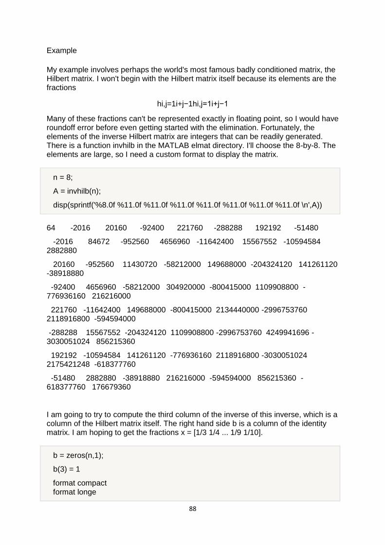
88

Example

My example involves perhaps the world's most famous badly conditioned matrix, the Hilbert matrix. I won't begin with the Hilbert matrix itself because its elements are the fractions

hi,j=1i+j−1hi,j=1i+j−1

Many of these fractions can't be represented exactly in floating point, so I would have roundoff error before even getting started with the elimination. Fortunately, the elements of the inverse Hilbert matrix are integers that can be readily generated. There is a function invhilb in the MATLAB elmat directory. I'll choose the 8-by-8. The elements are large, so I need a custom format to display the matrix.

n = 8;

A = invhilb(n);

disp(sprintf('%8.0f %11.0f %11.0f %11.0f %11.0f %11.0f %11.0f %11.0f \n',A))

64 -2016 20160 -92400 221760 -288288 192192 -51480

-2016 84672 -952560 4656960 -11642400 15567552 -10594584 2882880

20160 -952560 11430720 -58212000 149688000 -204324120 141261120 -38918880

-92400 4656960 -58212000 304920000 -800415000 1109908800 -776936160 216216000

221760 -11642400 149688000 -800415000 2134440000 -2996753760 2118916800 -594594000

-288288 15567552 -204324120 1109908800 -2996753760 4249941696 -3030051024 856215360

192192 -10594584 141261120 -776936160 2118916800 -3030051024 2175421248 -618377760

-51480 2882880 -38918880 216216000 -594594000 856215360 -618377760 176679360

I am going to try to compute the third column of the inverse of this inverse, which is a column of the Hilbert matrix itself. The right hand side b is a column of the identity matrix. I am hoping to get the fractions x = [1/3 1/4 ... 1/9 1/10].

b = zeros(n,1);

b(3) = 1

format compact format longe

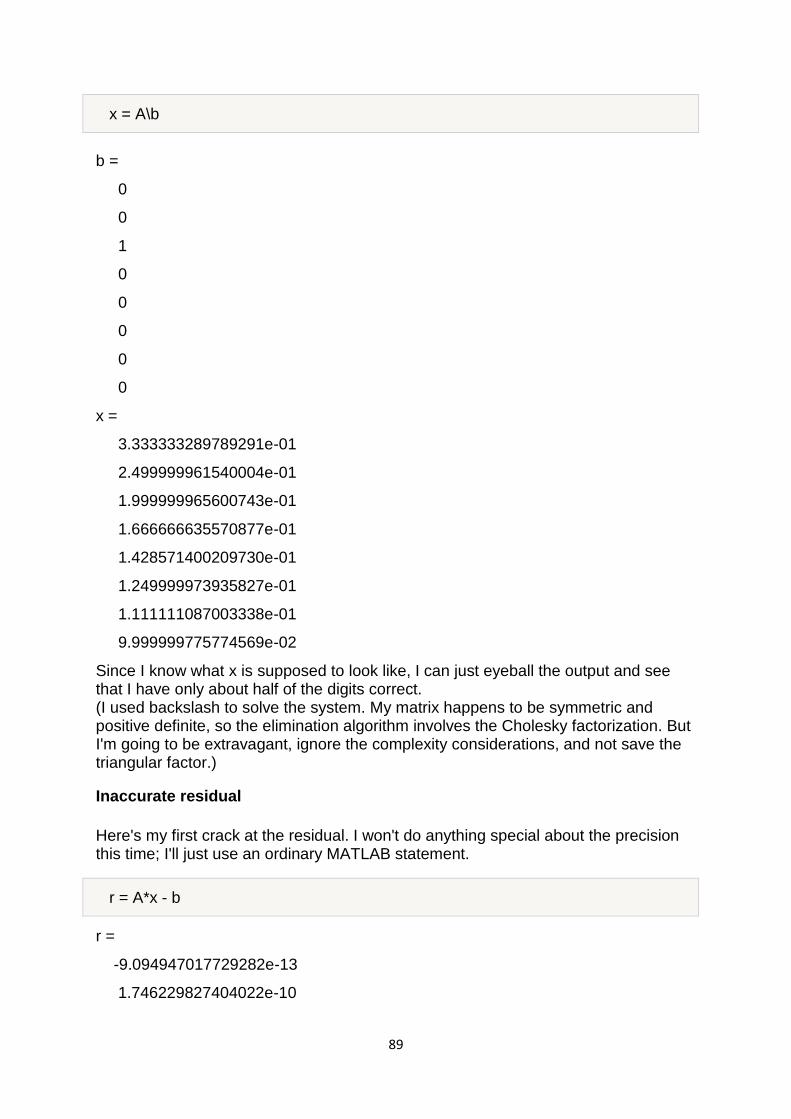
89

x = A\b

b =

0

0

1

0

0

0

0

0

x =

3.333333289789291e-01

2.499999961540004e-01

1.999999965600743e-01

1.666666635570877e-01

1.428571400209730e-01

1.249999973935827e-01

1.111111087003338e-01

9.999999775774569e-02

Since I know what x is supposed to look like, I can just eyeball the output and see that I have only about half of the digits correct. (I used backslash to solve the system. My matrix happens to be symmetric and positive definite, so the elimination algorithm involves the Cholesky factorization. But I'm going to be extravagant, ignore the complexity considerations, and not save the triangular factor.)

Inaccurate residual

Here's my first crack at the residual. I won't do anything special about the precision this time; I'll just use an ordinary MATLAB statement.

r = A*x - b

r =

-9.094947017729282e-13

1.746229827404022e-10

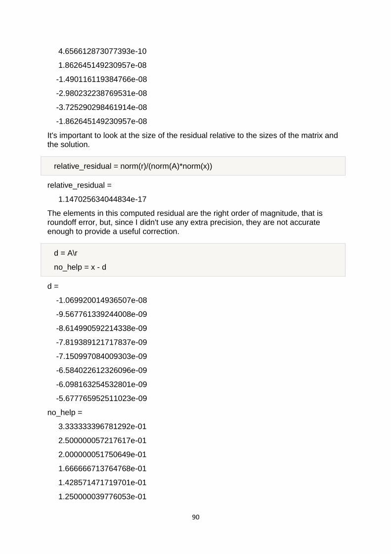
90

4.656612873077393e-10

1.862645149230957e-08

-1.490116119384766e-08

-2.980232238769531e-08

-3.725290298461914e-08

-1.862645149230957e-08

It's important to look at the size of the residual relative to the sizes of the matrix and the solution.

relative_residual = norm(r)/(norm(A)*norm(x))

relative_residual =

1.147025634044834e-17

The elements in this computed residual are the right order of magnitude, that is roundoff error, but, since I didn't use any extra precision, they are not accurate enough to provide a useful correction.

d = A\r

no_help = x - d

d =

-1.069920014936507e-08

-9.567761339244008e-09

-8.614990592214338e-09

-7.819389121717837e-09

-7.150997084009303e-09

-6.584022612326096e-09

-6.098163254532801e-09

-5.677765952511023e-09

no_help =

3.333333396781292e-01

2.500000057217617e-01

2.000000051750649e-01

1.666666713764768e-01

1.428571471719701e-01

1.250000039776053e-01

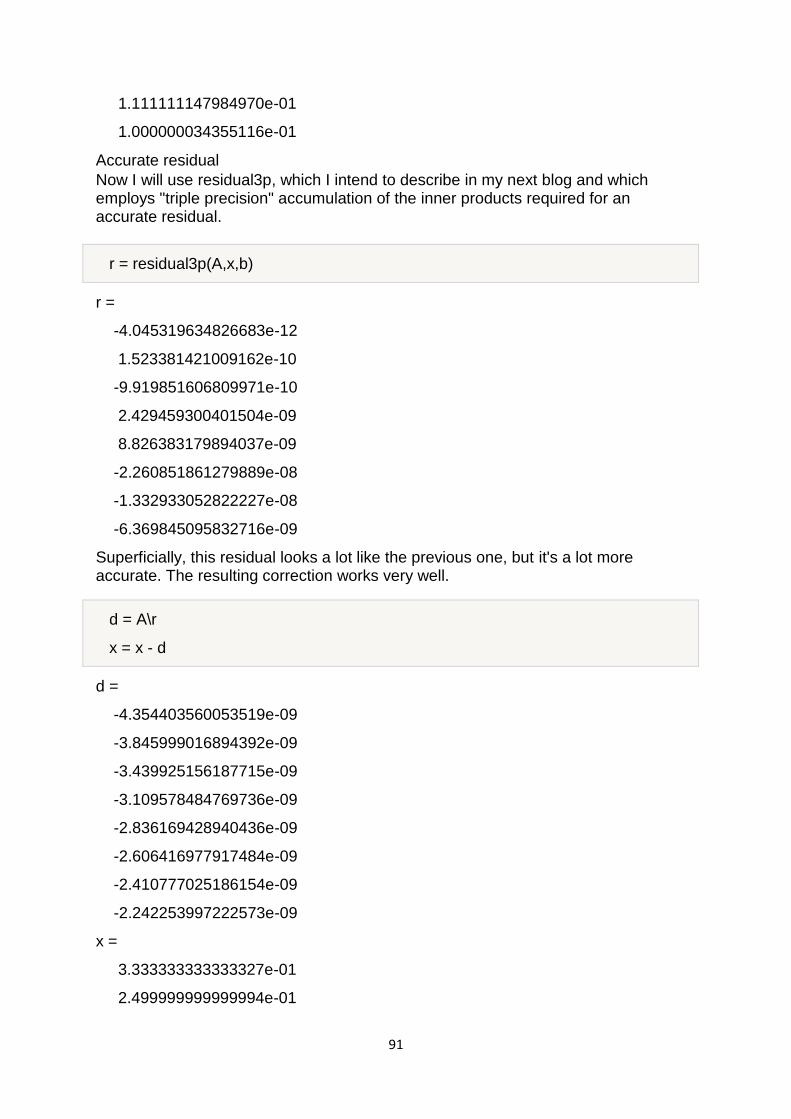
91

1.111111147984970e-01

1.000000034355116e-01

Accurate residual

Now I will use residual3p, which I intend to describe in my next blog and which employs "triple precision" accumulation of the inner products required for an accurate residual.

r = residual3p(A,x,b)

r =

-4.045319634826683e-12

1.523381421009162e-10

-9.919851606809971e-10

2.429459300401504e-09

8.826383179894037e-09

-2.260851861279889e-08

-1.332933052822227e-08

-6.369845095832716e-09

Superficially, this residual looks a lot like the previous one, but it's a lot more accurate. The resulting correction works very well.

d = A\r

x = x - d

d =

-4.354403560053519e-09

-3.845999016894392e-09

-3.439925156187715e-09

-3.109578484769736e-09

-2.836169428940436e-09

-2.606416977917484e-09

-2.410777025186154e-09

-2.242253997222573e-09

x =

3.333333333333327e-01

2.499999999999994e-01

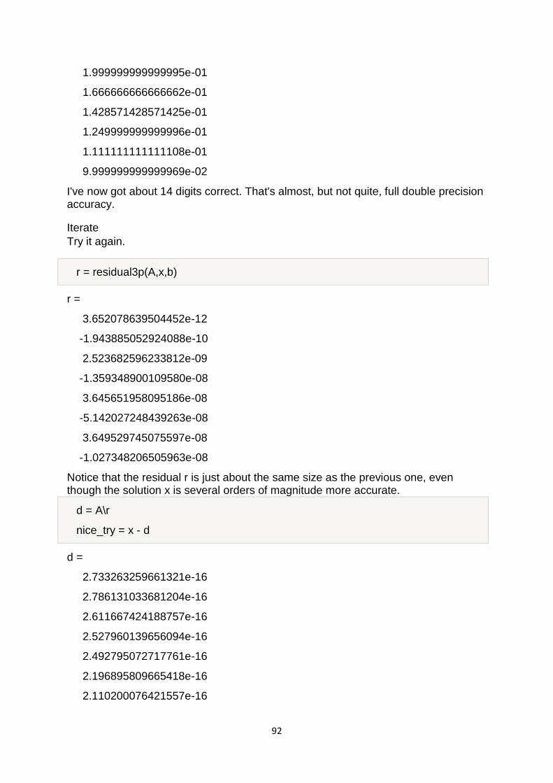
92

1.999999999999995e-01

1.666666666666662e-01

1.428571428571425e-01

1.249999999999996e-01

1.111111111111108e-01

9.999999999999969e-02

I've now got about 14 digits correct. That's almost, but not quite, full double precision accuracy.

Iterate

Try it again.

r = residual3p(A,x,b)

r =

3.652078639504452e-12

-1.943885052924088e-10

2.523682596233812e-09

-1.359348900109580e-08

3.645651958095186e-08

-5.142027248439263e-08

3.649529745075597e-08

-1.027348206505963e-08

Notice that the residual r is just about the same size as the previous one, even though the solution x is several orders of magnitude more accurate.

d = A\r

nice_try = x - d

d =

2.733263259661321e-16

2.786131033681204e-16

2.611667424188757e-16

2.527960139656094e-16

2.492795072717761e-16

2.196895809665418e-16

2.110200076421557e-16

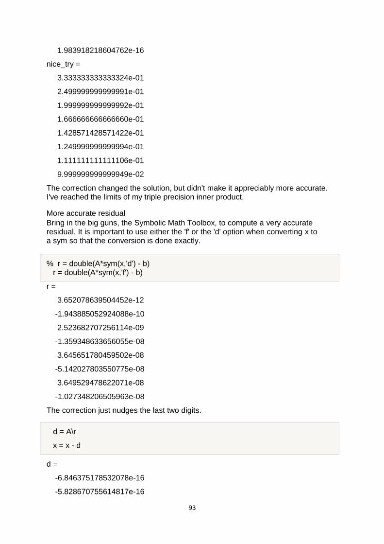
93

1.983918218604762e-16

nice_try =

3.333333333333324e-01

2.499999999999991e-01

1.999999999999992e-01

1.666666666666660e-01

1.428571428571422e-01

1.249999999999994e-01

1.111111111111106e-01

9.999999999999949e-02

The correction changed the solution, but didn't make it appreciably more accurate. I've reached the limits of my triple precision inner product.

More accurate residual

Bring in the big guns, the Symbolic Math Toolbox, to compute a very accurate residual. It is important to use either the 'f' or the 'd' option when converting x to a sym so that the conversion is done exactly.

% r = double(A*sym(x,'d') - b) r = double(A*sym(x,'f') - b)

r =

3.652078639504452e-12

-1.943885052924088e-10

2.523682707256114e-09

-1.359348633656055e-08

3.645651780459502e-08

-5.142027803550775e-08

3.649529478622071e-08

-1.027348206505963e-08

The correction just nudges the last two digits.

d = A\r

x = x - d

d =

-6.846375178532078e-16

-5.828670755614817e-16

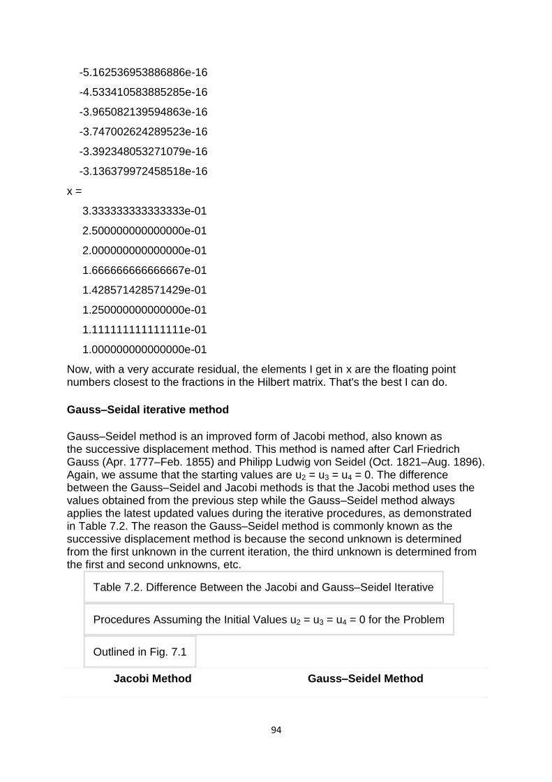
94

-5.162536953886886e-16

-4.533410583885285e-16

-3.965082139594863e-16

-3.747002624289523e-16

-3.392348053271079e-16

-3.136379972458518e-16

x =

3.333333333333333e-01

2.500000000000000e-01

2.000000000000000e-01

1.666666666666667e-01

1.428571428571429e-01

1.250000000000000e-01

1.111111111111111e-01

1.000000000000000e-01

Now, with a very accurate residual, the elements I get in x are the floating point numbers closest to the fractions in the Hilbert matrix. That's the best I can do.

Gauss–Seidal iterative method

Gauss–Seidel method is an improved form of Jacobi method, also known as the successive displacement method. This method is named after Carl Friedrich Gauss (Apr. 1777–Feb. 1855) and Philipp Ludwig von Seidel (Oct. 1821–Aug. 1896). Again, we assume that the starting values are u2 = u3 = u4 = 0. The difference between the Gauss–Seidel and Jacobi methods is that the Jacobi method uses the values obtained from the previous step while the Gauss–Seidel method always applies the latest updated values during the iterative procedures, as demonstrated in Table 7.2. The reason the Gauss–Seidel method is commonly known as the successive displacement method is because the second unknown is determined from the first unknown in the current iteration, the third unknown is determined from the first and second unknowns, etc.

Table 7.2. Difference Between the Jacobi and Gauss–Seidel Iterative

Procedures Assuming the Initial Values u2 = u3 = u4 = 0 for the Problem

Outlined in Fig. 7.1

Jacobi Method Gauss–Seidel Method

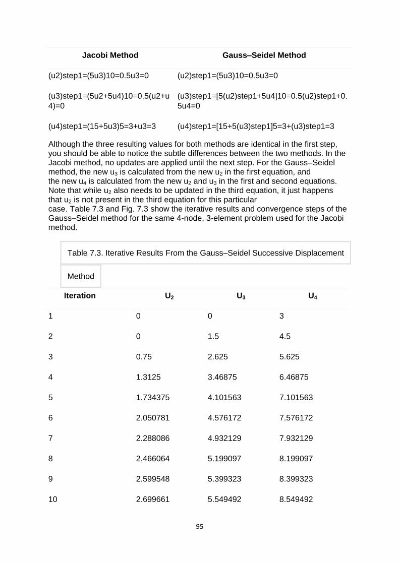
95

Jacobi Method Gauss–Seidel Method

(u2)step1=(5u3)10=0.5u3=0 (u2)step1=(5u3)10=0.5u3=0

(u3)step1=(5u2+5u4)10=0.5(u2+u

4)=0

(u3)step1=[5(u2)step1+5u4]10=0.5(u2)step1+0.

5u4=0

(u4)step1=(15+5u3)5=3+u3=3 (u4)step1=[15+5(u3)step1]5=3+(u3)step1=3

Although the three resulting values for both methods are identical in the first step, you should be able to notice the subtle differences between the two methods. In the Jacobi method, no updates are applied until the next step. For the Gauss–Seidel method, the new u3 is calculated from the new u2 in the first equation, and the new u4 is calculated from the new u2 and u3 in the first and second equations. Note that while u2 also needs to be updated in the third equation, it just happens that u2 is not present in the third equation for this particular case. Table 7.3 and Fig. 7.3 show the iterative results and convergence steps of the Gauss–Seidel method for the same 4-node, 3-element problem used for the Jacobi method.

Table 7.3. Iterative Results From the Gauss–Seidel Successive Displacement

Method

Iteration U2 U3 U4

1 0 0 3

2 0 1.5 4.5

3 0.75 2.625 5.625

4 1.3125 3.46875 6.46875

5 1.734375 4.101563 7.101563

6 2.050781 4.576172 7.576172

7 2.288086 4.932129 7.932129

8 2.466064 5.199097 8.199097

9 2.599548 5.399323 8.399323

10 2.699661 5.549492 8.549492

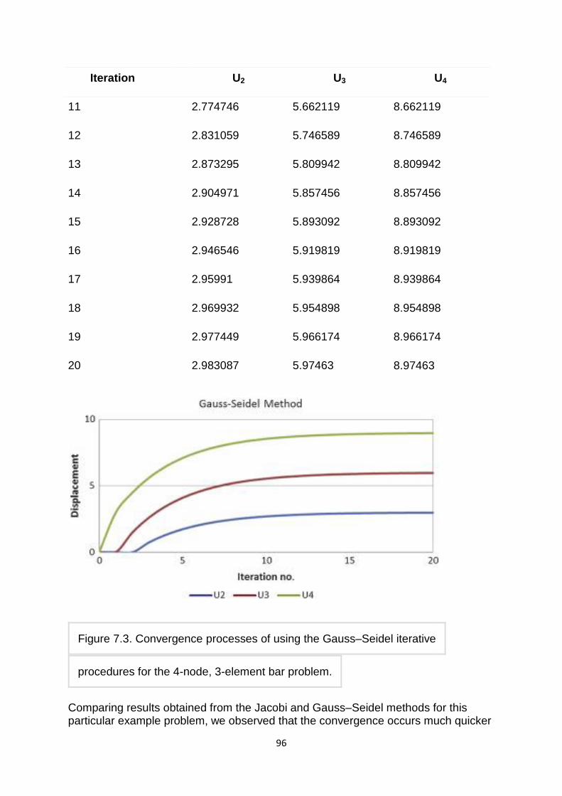
96

Iteration U2 U3 U4

11 2.774746 5.662119 8.662119

12 2.831059 5.746589 8.746589

13 2.873295 5.809942 8.809942

14 2.904971 5.857456 8.857456

15 2.928728 5.893092 8.893092

16 2.946546 5.919819 8.919819

17 2.95991 5.939864 8.939864

18 2.969932 5.954898 8.954898

19 2.977449 5.966174 8.966174

20 2.983087 5.97463 8.97463

Figure 7.3. Convergence processes of using the Gauss–Seidel iterative

procedures for the 4-node, 3-element bar problem.

Comparing results obtained from the Jacobi and Gauss–Seidel methods for this particular example problem, we observed that the convergence occurs much quicker

97

for the Gauss–Seidel method. Although this is true in most problems, some special cases may have opposite results. In terms of computational efficiency, the simultaneous displacement (Jacobi) method is perfectly designed for parallel computing, because none of the variables within each iteration change until the iteration is completed. As such, all variables need to be stored in memory until the iteration is finished. On the other hand, the Gauss–Seidel method can replace each variable as soon as a new update becomes available. Other iterative procedures apply different and yet conceptually similar approaches. Thus, no further discussion is made regarding other iterative solvers. As seen in the two iterative procedures shown above, iterative methods slowly reach the final solution rather than a large final step, as seen in the backward substitution procedures of the Gauss elimination. In summary, the direct method requires more in-core computer memory, but the solutions are accurate. On the other hand, the indirect method reaches the final solution gradually. However, as the level of convergence can be set by the users, a lower precision may be desired in order to detect the potential trend of the changing design variables much quicker than the direct method can provide.

Iterative Methods of Solution

Jonathan M. Blackledget, in Digital Signal Processing (Second Edition), 2006 9.1.2 The Gauss-Seidel Method

The Gauss-Seidel method involves updating the sub-diagonal elements as the computation proceeds. The iteration process is

x1k+1=1a11b1−a12x2k−…−a1nxnk,x2k+1=1a22b2−a21x1k+1−…−a2nxnk,⋮xnk+1=1

annbn−an1x1k+1−…−ann−1xn−1k+1.

Solution to a System of Linear Algebraic Equations

Sandip Mazumder, in Numerical Methods for Partial Differential Equations, 2016

3.2.3 Gauss–Seidel method

The Gauss–Seidel method is also a point-wise iteration method and bears a strong resemblance to the Jacobi method, but with one notable exception. In the Gauss–Seidel method, instead of always using previous iteration values for all terms of the right-hand side of Eq. (3.31), whenever an updated value becomes available, it is immediately used. Thus, for the 3×3 example system considered earlier [Eq. (3.17)] when x is determined using Eq. (3.17a), both y and z assume previous iteration values. However, when y is determined using Eq. (3.17b), only z assumes a previous iteration value. For x, the most recent value, which happens to be the current iteration value (since it has already been updated), is used. In the context of solution of a 2D PDE on a structured mesh, if the node by node update pattern (or sweeping pattern) is from left to right and bottom to top, as shown in Fig. 3.3(a), then, by the time it is node O‘s turn to get updated, nodes W and S have already been updated, and these updated values must be used. Essentially, this implies that

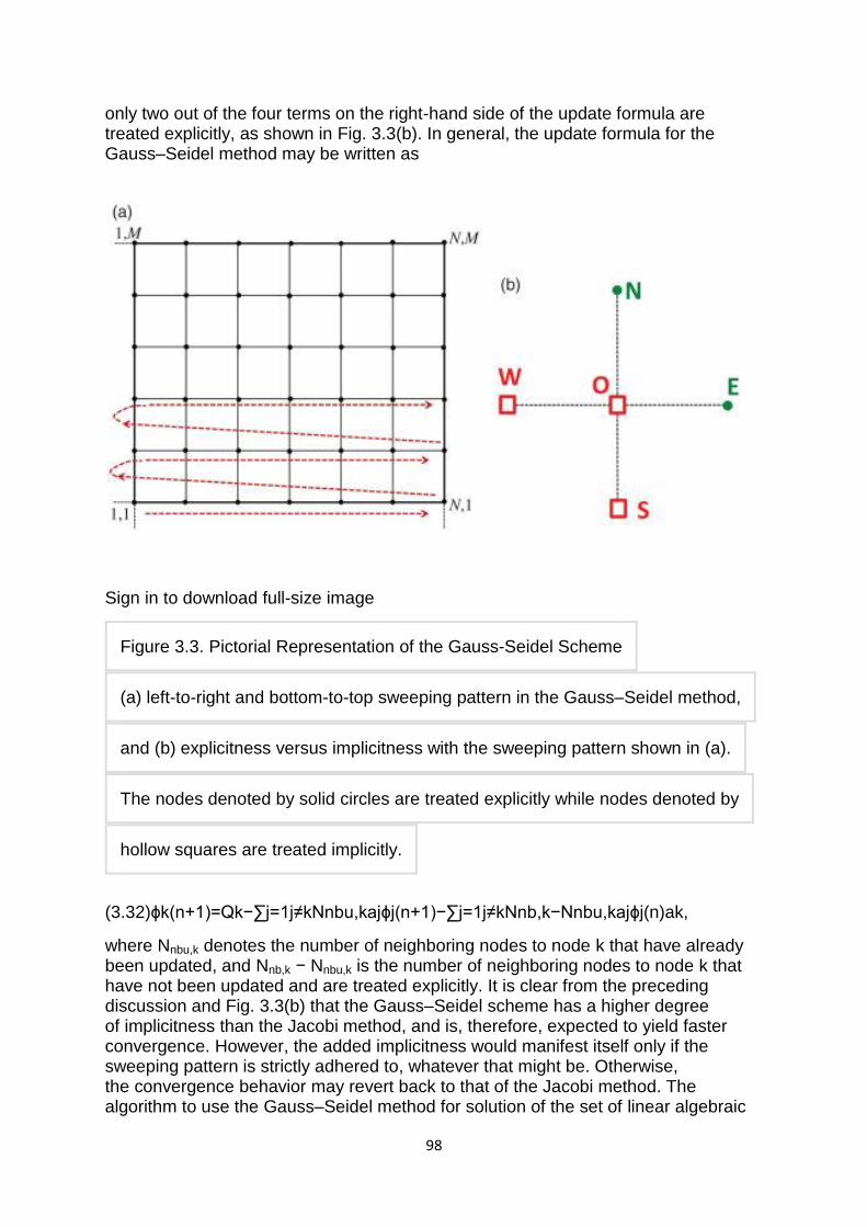
98

only two out of the four terms on the right-hand side of the update formula are treated explicitly, as shown in Fig. 3.3(b). In general, the update formula for the Gauss–Seidel method may be written as

Sign in to download full-size image

Figure 3.3. Pictorial Representation of the Gauss-Seidel Scheme

(a) left-to-right and bottom-to-top sweeping pattern in the Gauss–Seidel method,

and (b) explicitness versus implicitness with the sweeping pattern shown in (a).

The nodes denoted by solid circles are treated explicitly while nodes denoted by

hollow squares are treated implicitly.

(3.32)ϕk(n+1)=Qk−∑j=1j≠kNnbu,kajϕj(n+1)−∑j=1j≠kNnb,k−Nnbu,kajϕj(n)ak,

where Nnbu,k denotes the number of neighboring nodes to node k that have already been updated, and Nnb,k − Nnbu,k is the number of neighboring nodes to node k that have not been updated and are treated explicitly. It is clear from the preceding discussion and Fig. 3.3(b) that the Gauss–Seidel scheme has a higher degree of implicitness than the Jacobi method, and is, therefore, expected to yield faster convergence. However, the added implicitness would manifest itself only if the sweeping pattern is strictly adhered to, whatever that might be. Otherwise, the convergence behavior may revert back to that of the Jacobi method. The algorithm to use the Gauss–Seidel method for solution of the set of linear algebraic

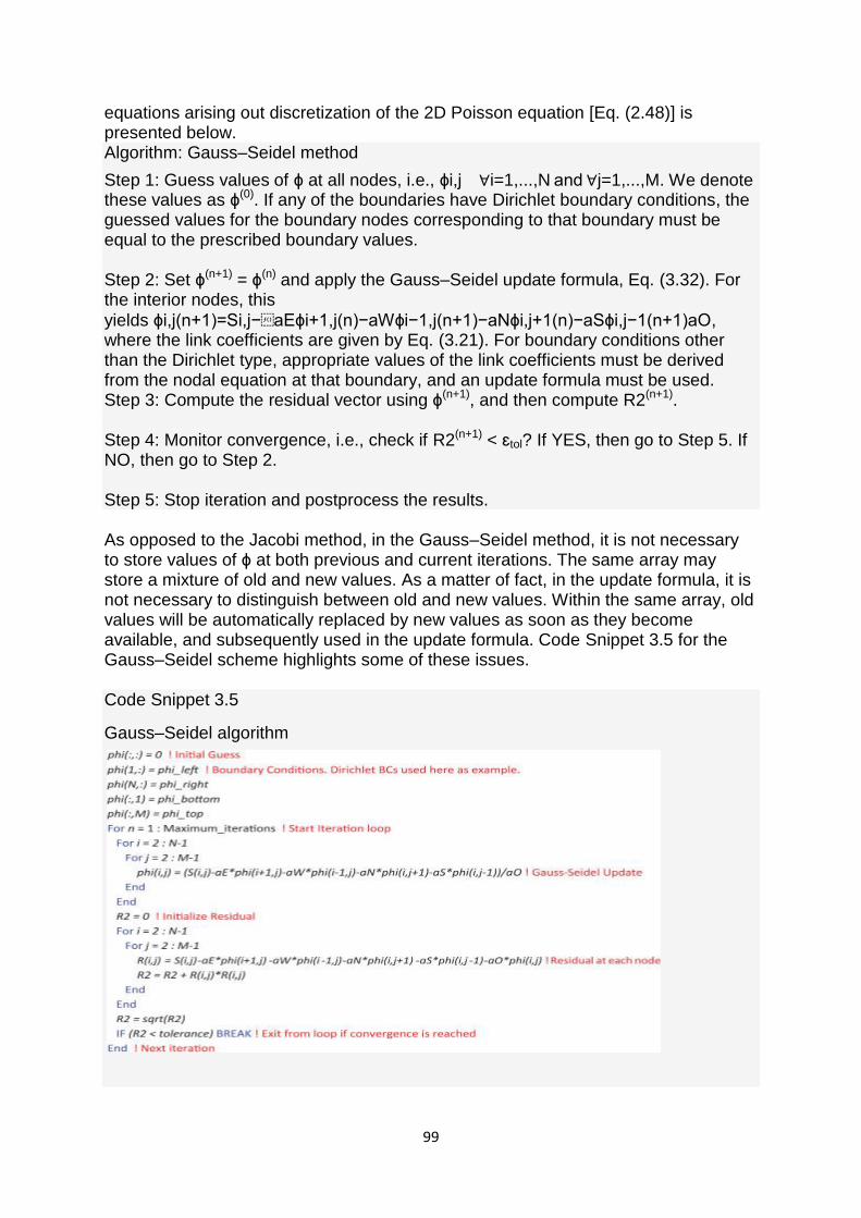
99

equations arising out discretization of the 2D Poisson equation [Eq. (2.48)] is presented below. Algorithm: Gauss–Seidel method

Step 1: Guess values of ϕ at all nodes, i.e., ϕi,j ∀i=1,...,N and ∀j=1,...,M. We denote these values as ϕ(0). If any of the boundaries have Dirichlet boundary conditions, the guessed values for the boundary nodes corresponding to that boundary must be equal to the prescribed boundary values. Step 2: Set ϕ(n+1) = ϕ(n) and apply the Gauss–Seidel update formula, Eq. (3.32). For the interior nodes, this

yields ϕi,j(n+1)=Si,j−aEϕi+1,j(n)−aWϕi−1,j(n+1)−aNϕi,j+1(n)−aSϕi,j−1(n+1)aO, where the link coefficients are given by Eq. (3.21). For boundary conditions other than the Dirichlet type, appropriate values of the link coefficients must be derived from the nodal equation at that boundary, and an update formula must be used. Step 3: Compute the residual vector using ϕ(n+1), and then compute R2(n+1). Step 4: Monitor convergence, i.e., check if R2(n+1) < ɛtol? If YES, then go to Step 5. If NO, then go to Step 2. Step 5: Stop iteration and postprocess the results. As opposed to the Jacobi method, in the Gauss–Seidel method, it is not necessary to store values of ϕ at both previous and current iterations. The same array may store a mixture of old and new values. As a matter of fact, in the update formula, it is not necessary to distinguish between old and new values. Within the same array, old values will be automatically replaced by new values as soon as they become available, and subsequently used in the update formula. Code Snippet 3.5 for the Gauss–Seidel scheme highlights some of these issues. Code Snippet 3.5

Gauss–Seidel algorithm

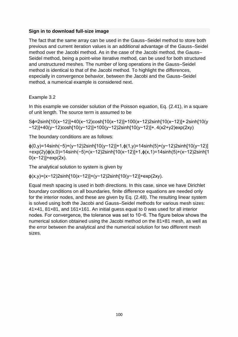
100

Sign in to download full-size image

The fact that the same array can be used in the Gauss–Seidel method to store both

previous and current iteration values is an additional advantage of the Gauss–Seidel

method over the Jacobi method. As in the case of the Jacobi method, the Gauss–

Seidel method, being a point-wise iterative method, can be used for both structured

and unstructured meshes. The number of long operations in the Gauss–Seidel

method is identical to that of the Jacobi method. To highlight the differences,

especially in convergence behavior, between the Jacobi and the Gauss–Seidel

method, a numerical example is considered next.

Example 3.2

In this example we consider solution of the Poisson equation, Eq. (2.41), in a square

of unit length. The source term is assumed to be

Sϕ=2sinh[10(x−12)]+40(x−12)cosh[10(x−12)]+100(x−12)2sinh[10(x−12)]+ 2sinh[10(y

−12)]+40(y−12)cosh[10(y−12)]+100(y−12)2sinh[10(y−12)]+. 4(x2+y2)exp(2xy)

The boundary conditions are as follows:

ϕ(0,y)=14sinh(−5)+(y−12)2sinh[10(y−12)]+1,ϕ(1,y)=14sinh(5)+(y−12)2sinh[10(y−12)]

+exp(2y)ϕ(x,0)=14sinh(−5)+(x−12)2sinh[10(x−12)]+1,ϕ(x,1)=14sinh(5)+(x−12)2sinh[1

0(x−12)]+exp(2x).

The analytical solution to system is given by

ϕ(x,y)=(x−12)2sinh[10(x−12)]+(y−12)2sinh[10(y−12)]+exp(2xy).

Equal mesh spacing is used in both directions. In this case, since we have Dirichlet

boundary conditions on all boundaries, finite difference equations are needed only

for the interior nodes, and these are given by Eq. (2.48). The resulting linear system

is solved using both the Jacobi and Gauss–Seidel methods for various mesh sizes:

41×41, 81×81, and 161×161. An initial guess equal to 0 was used for all interior

nodes. For convergence, the tolerance was set to 10−6. The figure below shows the

numerical solution obtained using the Jacobi method on the 81×81 mesh, as well as

the error between the analytical and the numerical solution for two different mesh

sizes.

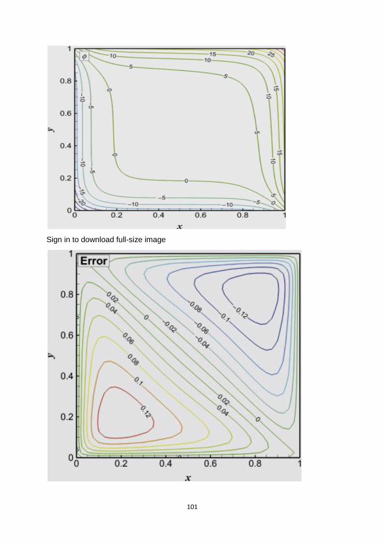
101

Sign in to download full-size image

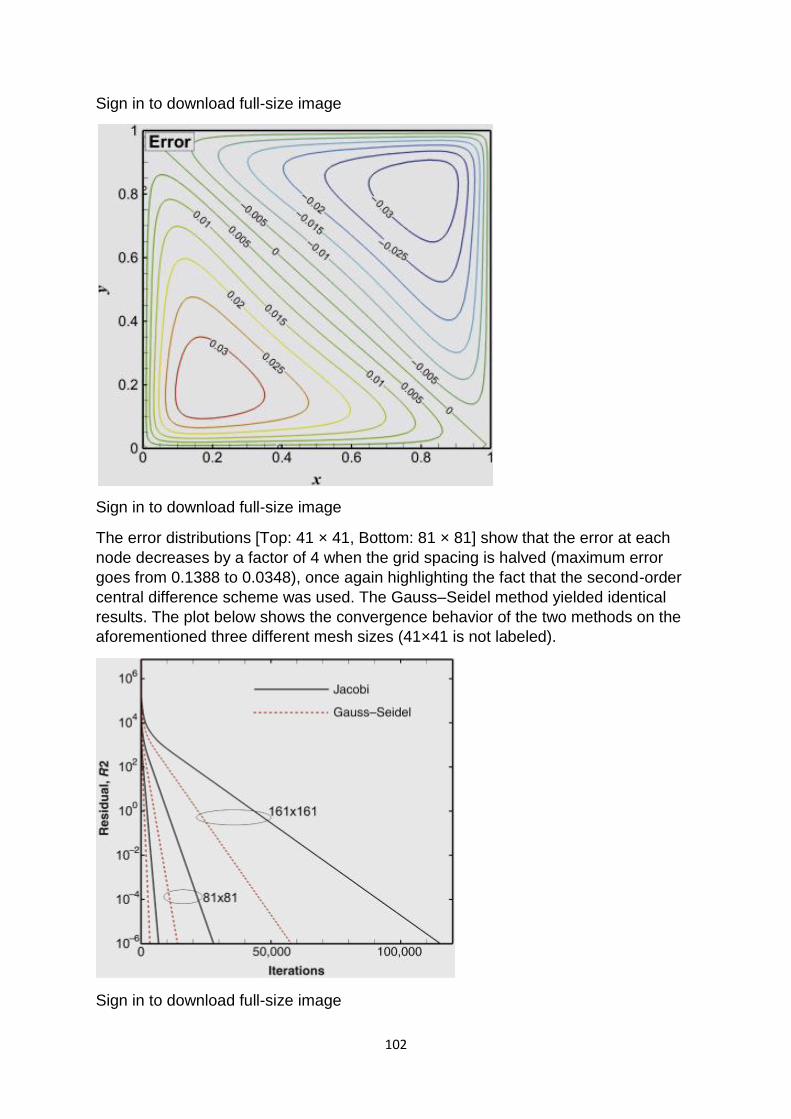
102

Sign in to download full-size image

Sign in to download full-size image

The error distributions [Top: 41 × 41, Bottom: 81 × 81] show that the error at each

node decreases by a factor of 4 when the grid spacing is halved (maximum error

goes from 0.1388 to 0.0348), once again highlighting the fact that the second-order

central difference scheme was used. The Gauss–Seidel method yielded identical

results. The plot below shows the convergence behavior of the two methods on the

aforementioned three different mesh sizes (41×41 is not labeled).

Sign in to download full-size image

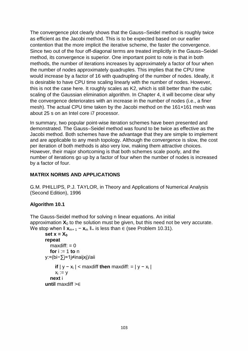
103

The convergence plot clearly shows that the Gauss–Seidel method is roughly twice

as efficient as the Jacobi method. This is to be expected based on our earlier

contention that the more implicit the iterative scheme, the faster the convergence.

Since two out of the four off-diagonal terms are treated implicitly in the Gauss–Seidel

method, its convergence is superior. One important point to note is that in both

methods, the number of iterations increases by approximately a factor of four when

the number of nodes approximately quadruples. This implies that the CPU time

would increase by a factor of 16 with quadrupling of the number of nodes. Ideally, it

is desirable to have CPU time scaling linearly with the number of nodes. However,

this is not the case here. It roughly scales as K2, which is still better than the cubic

scaling of the Gaussian elimination algorithm. In Chapter 4, it will become clear why

the convergence deteriorates with an increase in the number of nodes (i.e., a finer

mesh). The actual CPU time taken by the Jacobi method on the 161×161 mesh was

about 25 s on an Intel core i7 processor.

In summary, two popular point-wise iteration schemes have been presented and demonstrated. The Gauss–Seidel method was found to be twice as effective as the Jacobi method. Both schemes have the advantage that they are simple to implement and are applicable to any mesh topology. Although the convergence is slow, the cost per iteration of both methods is also very low, making them attractive choices. However, their major shortcoming is that both schemes scale poorly, and the number of iterations go up by a factor of four when the number of nodes is increased by a factor of four. MATRIX NORMS AND APPLICATIONS

G.M. PHILLIPS, P.J. TAYLOR, in Theory and Applications of Numerical Analysis (Second Edition), 1996 Algorithm 10.1

The Gauss-Seidel method for solving n linear equations. An initial approximation X0 to the solution must be given, but this need not be very accurate.

We stop when ‖ xm+ 1 − xm ‖∞ is less than ∈ (see Problem 10.31). set x = X0 repeat maxdiff: = 0 for i := 1 to n y:=(bi−∑j=1j≠inaijxj)/aii

if | y − xi | < maxdiff then maxdiff: = | y − xi | xi := y next i

until maxdiff >∈

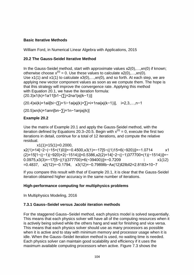
104

Basic Iterative Methods

William Ford, in Numerical Linear Algebra with Applications, 2015 20.2 The Gauss-Seidel Iterative Method

In the Gauss-Seidel method, start with approximate values x2(0),…,xn(0) if known; otherwise choose x(0) = 0. Use these values to calculate x2(0),…,xn(0). Use x1(1) and x1(1) to calculate x3(0),…,xn(0), and so forth. At each step, we are applying new vector component values as soon as we compute them. The hope is that this strategy will improve the convergence rate. Applying this method with Equation 20.1, we have the iteration formula: (20.3)x1(k)=1a11[b1−(∑j=2na1jxj(k−1))]

(20.4)xi(k)=1aii[bi−(∑j=1i−1aijxj(k)+∑j=i+1naijxj(k−1))], i=2,3,…,n−1

(20.5)xn(k)=1ann[bn−∑j=1n−1anjxj(k)]

Example 20.2 Use the matrix of Example 20.1 and apply the Gauss-Seidel method, with the iteration defined by Equations 20.3–20.5. Begin with x(0) = 0, execute the first two iterations in detail, continue for a total of 12 iterations, and compute the relative residual.                  x1(1)=15(1)=0.2000,

x2(1)=14[−2−(−15+(1)0)]=−0.4500,x3(1)=−17[5−((1)15+6(−920))]=−1.0714                x1

(2)=15[1−((−1)(−920)+2(−1514))]=0.5386,x2(2)=14[−2−((−1)377700+(1)(−1514))]=−

0.0975,x3(3)=−17[5−((1)(377700)+6(−39400))]=−0.7209                             ⋮                x1(12)

=0.4837, x2(12)=−0.1794, x3(12)=−0.7989‖b−Ax(12)‖2‖b‖2=2.8183×10−7

If you compare this result with that of Example 20.1, it is clear that the Gauss-Seidel iteration obtained higher accuracy in the same number of iterations. High-performance computing for multiphysics problems

In Multiphysics Modeling, 2016 7.3.1 Gauss–Seidel versus Jacobi iteration methods

For the staggered Gauss–Seidel method, each physics model is solved sequentially. This means that each physics solver will have all of the computing resources when it is actively being solved while the others hang and wait for finishing and vice versa. This means that each physics solver should use as many processors as possible when it is active and to stay with minimum memory and processor usage when it is idle. When the Gauss–Seidel iteration method is used, no waiting time is needed. Each physics solver can maintain good scalability and efficiency if it uses the maximum available computing processors when active. Figure 7.3 shows the

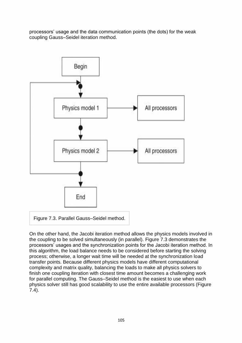
105

processors‘ usage and the data communication points (the dots) for the weak coupling Gauss–Seidel iteration method.

Figure 7.3. Parallel Gauss–Seidel method.

On the other hand, the Jacobi iteration method allows the physics models involved in the coupling to be solved simultaneously (in parallel). Figure 7.3 demonstrates the processors‘ usages and the synchronization points for the Jacobi iteration method. In this algorithm, the load balance needs to be considered before starting the solving process; otherwise, a longer wait time will be needed at the synchronization load transfer points. Because different physics models have different computational complexity and matrix quality, balancing the loads to make all physics solvers to finish one coupling iteration with closest time amount becomes a challenging work for parallel computing. The Gauss–Seidel method is the easiest to use when each physics solver still has good scalability to use the entire available processors (Figure 7.4).

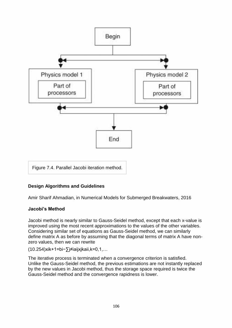
106

Figure 7.4. Parallel Jacobi iteration method.

Design Algorithms and Guidelines

Amir Sharif Ahmadian, in Numerical Models for Submerged Breakwaters, 2016

Jacobi’s Method

Jacobi method is nearly similar to Gauss-Seidel method, except that each x-value is improved using the most recent approximations to the values of the other variables. Considering similar set of equations as Gauss-Seidel method, we can similarly define matrix A as before by assuming that the diagonal terms of matrix A have non-zero values, then we can rewrite

(10.254)xik+1=bi−∑j≠iaijxjkaii,k=0,1,…

The iterative process is terminated when a convergence criterion is satisfied. Unlike the Gauss-Seidel method, the previous estimations are not instantly replaced by the new values in Jacobi method, thus the storage space required is twice the Gauss-Seidel method and the convergence rapidness is lower.

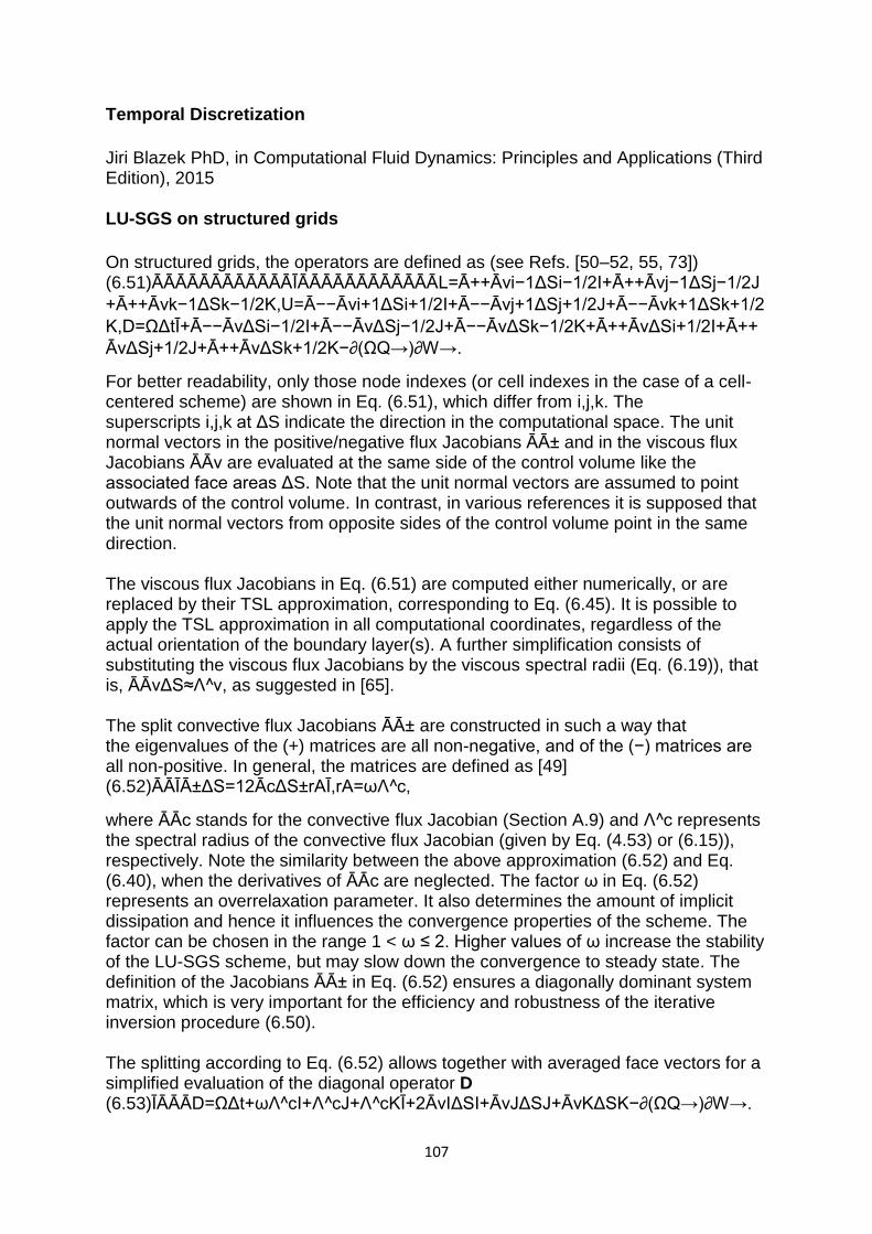
107

Temporal Discretization

Jiri Blazek PhD, in Computational Fluid Dynamics: Principles and Applications (Third Edition), 2015 LU-SGS on structured grids

On structured grids, the operators are defined as (see Refs. [50–52, 55, 73]) (6.51)ĀĀĀĀĀĀĀĀĀĀĀĀĪĀĀĀĀĀĀĀĀĀĀĀĀL=Ā++Āvi−1ΔSi−1/2I+Ā++Āvj−1ΔSj−1/2J

+Ā++Āvk−1ΔSk−1/2K,U=Ā−−Āvi+1ΔSi+1/2I+Ā−−Āvj+1ΔSj+1/2J+Ā−−Āvk+1ΔSk+1/2

K,D=ΩΔtĪ+Ā−−ĀvΔSi−1/2I+Ā−−ĀvΔSj−1/2J+Ā−−ĀvΔSk−1/2K+Ā++ĀvΔSi+1/2I+Ā++

ĀvΔSj+1/2J+Ā++ĀvΔSk+1/2K−∂(ΩQ→)∂W→.

For better readability, only those node indexes (or cell indexes in the case of a cell-centered scheme) are shown in Eq. (6.51), which differ from i,j,k. The superscripts i,j,k at ΔS indicate the direction in the computational space. The unit normal vectors in the positive/negative flux Jacobians ĀĀ± and in the viscous flux Jacobians ĀĀv are evaluated at the same side of the control volume like the associated face areas ΔS. Note that the unit normal vectors are assumed to point outwards of the control volume. In contrast, in various references it is supposed that the unit normal vectors from opposite sides of the control volume point in the same direction. The viscous flux Jacobians in Eq. (6.51) are computed either numerically, or are replaced by their TSL approximation, corresponding to Eq. (6.45). It is possible to apply the TSL approximation in all computational coordinates, regardless of the actual orientation of the boundary layer(s). A further simplification consists of substituting the viscous flux Jacobians by the viscous spectral radii (Eq. (6.19)), that is, ĀĀvΔS≈Λ^v, as suggested in [65]. The split convective flux Jacobians ĀĀ± are constructed in such a way that the eigenvalues of the (+) matrices are all non-negative, and of the (−) matrices are all non-positive. In general, the matrices are defined as [49] (6.52)ĀĀĪĀ±ΔS=12ĀcΔS±rAĪ,rA=ωΛ^c,

where ĀĀc stands for the convective flux Jacobian (Section A.9) and Λ^c represents the spectral radius of the convective flux Jacobian (given by Eq. (4.53) or (6.15)), respectively. Note the similarity between the above approximation (6.52) and Eq. (6.40), when the derivatives of ĀĀc are neglected. The factor ω in Eq. (6.52) represents an overrelaxation parameter. It also determines the amount of implicit dissipation and hence it influences the convergence properties of the scheme. The factor can be chosen in the range 1 < ω ≤ 2. Higher values of ω increase the stability of the LU-SGS scheme, but may slow down the convergence to steady state. The definition of the Jacobians ĀĀ± in Eq. (6.52) ensures a diagonally dominant system matrix, which is very important for the efficiency and robustness of the iterative inversion procedure (6.50). The splitting according to Eq. (6.52) allows together with averaged face vectors for a simplified evaluation of the diagonal operator D (6.53)ĪĀĀĀD=ΩΔt+ωΛ^cI+Λ^cJ+Λ^cKĪ+2ĀvIΔSI+ĀvJΔSJ+ĀvKΔSK−∂(ΩQ→)∂W→.

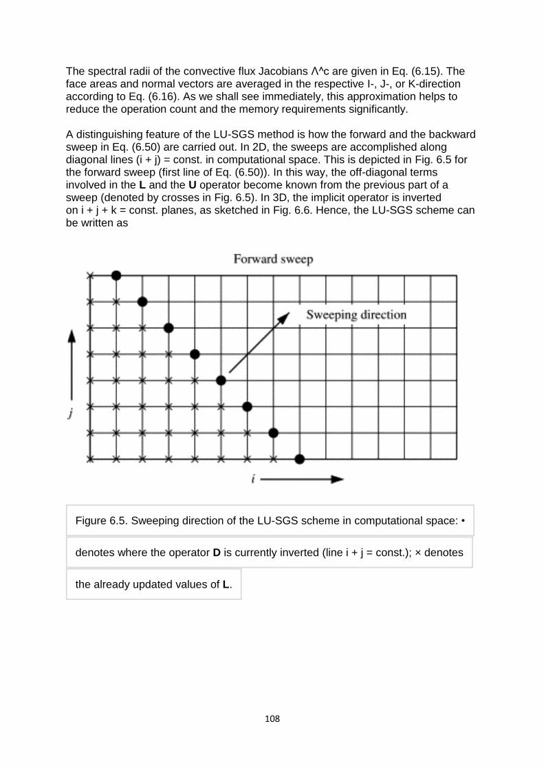
108

The spectral radii of the convective flux Jacobians Λ^c are given in Eq. (6.15). The face areas and normal vectors are averaged in the respective I-, J-, or K-direction according to Eq. (6.16). As we shall see immediately, this approximation helps to reduce the operation count and the memory requirements significantly. A distinguishing feature of the LU-SGS method is how the forward and the backward sweep in Eq. (6.50) are carried out. In 2D, the sweeps are accomplished along diagonal lines (i + j) = const. in computational space. This is depicted in Fig. 6.5 for the forward sweep (first line of Eq. (6.50)). In this way, the off-diagonal terms involved in the L and the U operator become known from the previous part of a sweep (denoted by crosses in Fig. 6.5). In 3D, the implicit operator is inverted on i + j + k = const. planes, as sketched in Fig. 6.6. Hence, the LU-SGS scheme can be written as

Figure 6.5. Sweeping direction of the LU-SGS scheme in computational space: •

denotes where the operator D is currently inverted (line i + j = const.); × denotes

the already updated values of L.

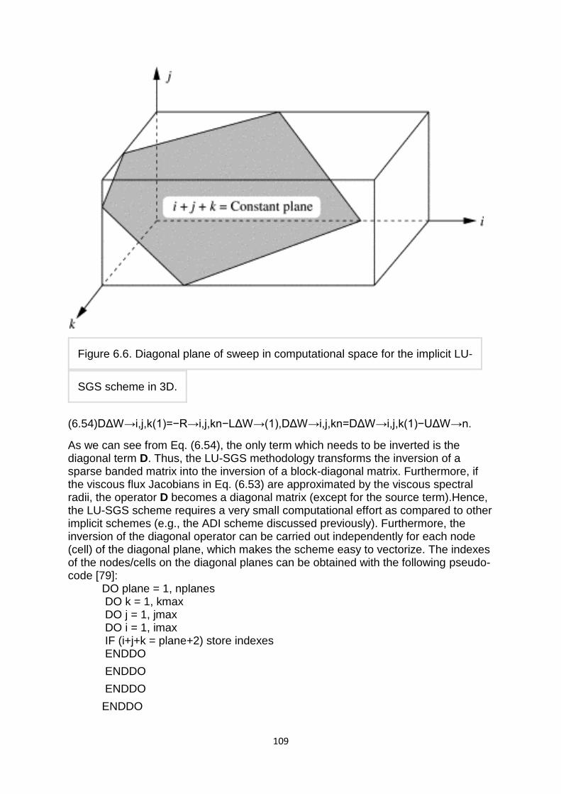
109

Figure 6.6. Diagonal plane of sweep in computational space for the implicit LU-

SGS scheme in 3D.

(6.54)DΔW→i,j,k(1)=−R→i,j,kn−LΔW→(1),DΔW→i,j,kn=DΔW→i,j,k(1)−UΔW→n.

As we can see from Eq. (6.54), the only term which needs to be inverted is the diagonal term D. Thus, the LU-SGS methodology transforms the inversion of a sparse banded matrix into the inversion of a block-diagonal matrix. Furthermore, if the viscous flux Jacobians in Eq. (6.53) are approximated by the viscous spectral radii, the operator D becomes a diagonal matrix (except for the source term).Hence, the LU-SGS scheme requires a very small computational effort as compared to other implicit schemes (e.g., the ADI scheme discussed previously). Furthermore, the inversion of the diagonal operator can be carried out independently for each node (cell) of the diagonal plane, which makes the scheme easy to vectorize. The indexes of the nodes/cells on the diagonal planes can be obtained with the following pseudo-code [79]:

DO plane = 1, nplanes DO k = 1, kmax DO j = 1, jmax DO i = 1, imax IF (i+j+k = plane+2) store indexes ENDDO

ENDDO

ENDDO

ENDDO

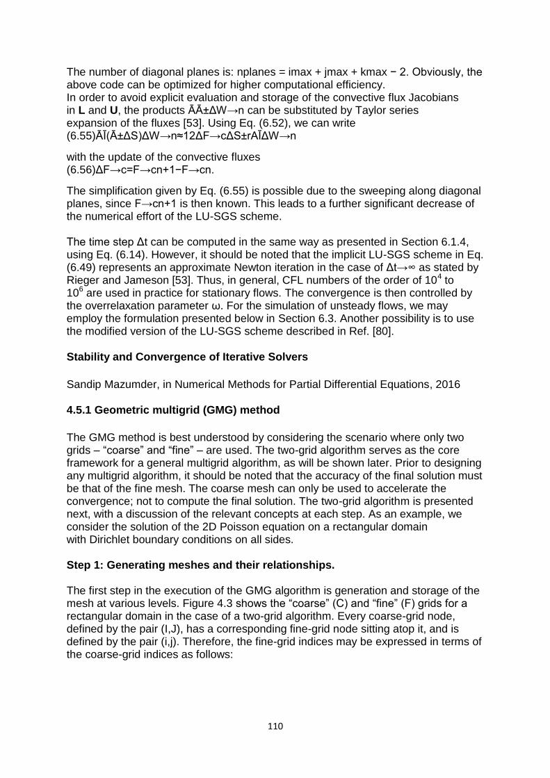
110

The number of diagonal planes is: nplanes = imax + jmax + kmax − 2. Obviously, the above code can be optimized for higher computational efficiency. In order to avoid explicit evaluation and storage of the convective flux Jacobians in L and U, the products ĀĀ±ΔW→n can be substituted by Taylor series expansion of the fluxes [53]. Using Eq. (6.52), we can write (6.55)ĀĪ(Ā±ΔS)ΔW→n≈12ΔF→cΔS±rAĪΔW→n

with the update of the convective fluxes (6.56)ΔF→c=F→cn+1−F→cn.

The simplification given by Eq. (6.55) is possible due to the sweeping along diagonal planes, since F→cn+1 is then known. This leads to a further significant decrease of the numerical effort of the LU-SGS scheme. The time step Δt can be computed in the same way as presented in Section 6.1.4, using Eq. (6.14). However, it should be noted that the implicit LU-SGS scheme in Eq. (6.49) represents an approximate Newton iteration in the case of Δt→∞ as stated by Rieger and Jameson [53]. Thus, in general, CFL numbers of the order of 104 to 106 are used in practice for stationary flows. The convergence is then controlled by the overrelaxation parameter ω. For the simulation of unsteady flows, we may employ the formulation presented below in Section 6.3. Another possibility is to use the modified version of the LU-SGS scheme described in Ref. [80]. Stability and Convergence of Iterative Solvers

Sandip Mazumder, in Numerical Methods for Partial Differential Equations, 2016 4.5.1 Geometric multigrid (GMG) method

The GMG method is best understood by considering the scenario where only two grids – ―coarse‖ and ―fine‖ – are used. The two-grid algorithm serves as the core framework for a general multigrid algorithm, as will be shown later. Prior to designing any multigrid algorithm, it should be noted that the accuracy of the final solution must be that of the fine mesh. The coarse mesh can only be used to accelerate the convergence; not to compute the final solution. The two-grid algorithm is presented next, with a discussion of the relevant concepts at each step. As an example, we consider the solution of the 2D Poisson equation on a rectangular domain with Dirichlet boundary conditions on all sides. Step 1: Generating meshes and their relationships. The first step in the execution of the GMG algorithm is generation and storage of the mesh at various levels. Figure 4.3 shows the ―coarse‖ (C) and ―fine‖ (F) grids for a rectangular domain in the case of a two-grid algorithm. Every coarse-grid node, defined by the pair (I,J), has a corresponding fine-grid node sitting atop it, and is defined by the pair (i,j). Therefore, the fine-grid indices may be expressed in terms of the coarse-grid indices as follows:

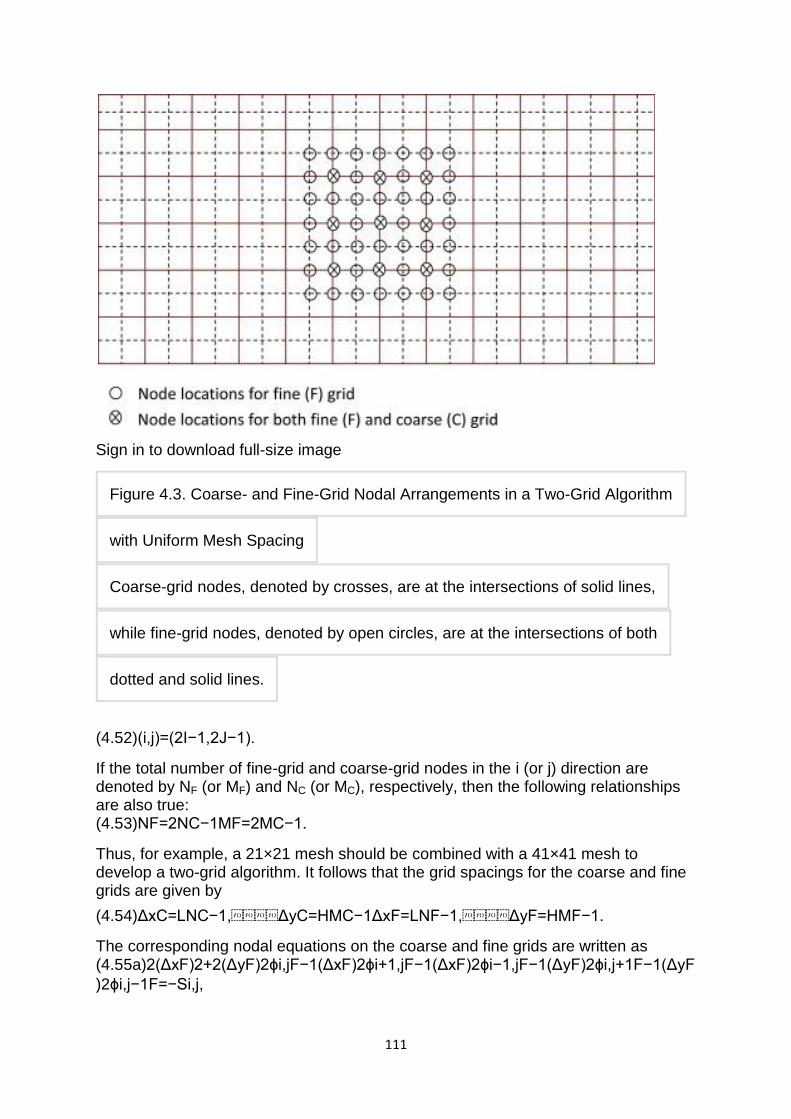
111

Sign in to download full-size image

Figure 4.3. Coarse- and Fine-Grid Nodal Arrangements in a Two-Grid Algorithm

with Uniform Mesh Spacing

Coarse-grid nodes, denoted by crosses, are at the intersections of solid lines,

while fine-grid nodes, denoted by open circles, are at the intersections of both

dotted and solid lines.

(4.52)(i,j)=(2I−1,2J−1).

If the total number of fine-grid and coarse-grid nodes in the i (or j) direction are denoted by NF (or MF) and NC (or MC), respectively, then the following relationships are also true: (4.53)NF=2NC−1MF=2MC−1.

Thus, for example, a 21×21 mesh should be combined with a 41×41 mesh to develop a two-grid algorithm. It follows that the grid spacings for the coarse and fine grids are given by

(4.54)ΔxC=LNC−1,ΔyC=HMC−1ΔxF=LNF−1,ΔyF=HMF−1.

The corresponding nodal equations on the coarse and fine grids are written as (4.55a)2(ΔxF)2+2(ΔyF)2ϕi,jF−1(ΔxF)2ϕi+1,jF−1(ΔxF)2ϕi−1,jF−1(ΔyF)2ϕi,j+1F−1(ΔyF

)2ϕi,j−1F=−Si,j,

112

(4.55b)2(ΔxC)2+2(ΔyC)2ϕI,JC−1(ΔxC)2ϕI+1,JC−1(ΔxC)2ϕI−1,JC−1(ΔyC)2ϕI,J+1C−

1(ΔyC)2ϕI,J−1C=−SI,J.

Step 2: Set initial guess The next step in the algorithm is to initialize the dependent variable on the fine grid. Since the fine-grid solution is what we are ultimately interested in, it is sufficient to initialize (guess) the solution at the fine-grid nodes. Let this solution be denoted by ϕi,jF(0). If Dirichlet boundary conditions are used, the initial guess at the boundary nodes should be set equal to the prescribed boundary value. Step 3: Smoothing on fine grid Next, the algebraic equations on the fine grid are solved using a solver of choice, but only to partial convergence. While any solver, discussed in Chapter 3, may be used for this purpose, it is important to choose one that is easy to implement and whose computational workload per iteration is small. This is because in the context of the GMG algorithm, the solver is not solely responsible for reducing the errors. Rather, the multigrid framework is. In other words, the overall iteration count is not dictated by the solver but rather by the multigrid treatment of the errors. The solver to be used is also known as the smoother, and the operation of solving the fine-grid equations to partial convergence is known as smoothing. Based on the criterion of low computational workload per iteration, it is customary to use classical iterative solvers for the smoothing operation rather than fully implicit solvers, such as the Krylov subspace solvers. The Gauss–Seidel method is a popular choice as the smoother for multigrid algorithms, primarily because of its extremely low workload per iteration, its ease of implementation, and also the fact that it can be used for both structured and unstructured mesh topologies. It is clear that solving the fine-grid equations to full convergence in this step would be tantamount to not using the multigrid method at all. Instead, the solution is taken only to partial convergence. To the best of the author‘s knowledge, there is no reported mathematical analysis that shows the optimum level of partial convergence that is universally applicable to all problems. Generally, iterations are continued until the R2F decreases by a factor of about two. Often, calculation and monitoring of the scaled residual, as would be required if the residual were to be decreased by a factor two, is completely bypassed, and one or two sweeps of Gauss–Seidel is executed instead. This makes the implementation even easier. At this point in the algorithm, the solution on the fine grid, ϕi,jF, contains errors due to partial convergence. This error (equal to the difference between the exact numerical solution and the solution at the current iteration) has several different wavelength components. As discussed in Section 4.2.1, of these, the components that have large wavelengths are the most difficult to damp out (or have their amplitudes reduced). Therefore, instead of continuing with regular smoothing (Gauss–Seidel iterations on the fine grid, for example), which would not specifically target the large wavelength components, we transfer this error to a coarse grid and then smooth it on the coarse grid so that they are reduced rapidly. In preparation for these actions, the following step is executed next.

113

Step 4: Computation of residual on fine grid The residual and L2Norm are computed on the fine grid using [R] F=[Q]−[A]F[ϕ]F, and R2 F=[R]FT[R]F. Step 5: Transfer of fine-grid residual to coarse grid (restriction) The residual computed on the fine grid in Step 4 is next transfered to the coarse grid. This process is known as restriction. Since every fine-grid node has a coarse-grid node sitting atop it, the restriction operation simply involves copying the residuals on the fine grid to an array (data structure) that stores residuals for the coarse grid. The loops used to perform this transfer should run over the indices of the coarse grid and Eq. (4.52) should be made use of to obtain corresponding fine-grid indices. Henceforth, the residual transferred from the fine to the coarse grid will be denoted by [R]C←F. For a more complex grid structure, the coarse- and fine-grid nodes may not always overlap. In such a scenario, interpolation will be necessary to execute the transfer process. Step 6: Smoothing on coarse grid The transferred residuals are next smoothed on the coarse grid with the specific intent to damp out the large wavelength components of the error rapidly. This operation entails solution of the equation [A]C[ϕ′]C=[R]C←F to partial convergence, where [A]C is the coefficient matrix computed on the coarse mesh [see Eq. (4.55b)] and [ϕ′]C is the predicted correction on the coarse mesh. As in Step 3, a solver with a low computational workload and one that is easy to implement must be used. The equation [A]C[ϕ′]C=[R]C←F essentially represents the governing linear system in correction form (see Section 3.2.1). Generally, tighter tolerance or more sweeps (typically two or three, as opposed to one) is needed in this step than in Step 3 to obtain an accurate enough prediction of the correction. The Gauss–Seidel method is also a commonly used method for this step. Step 7: Transfer of coarse-grid correction to fine grid (prolongation) The correction obtained on the coarse grid, [ϕ']C, is next transferred to the fine grid. This process is known as prolongation. Execution of the prolongation step involves interpolation since all fine-grid nodes do not have coarse-grid nodes sitting atop them. The transfer of [ϕ']C can be classified into three categories. For the fine-grid nodes that have coarse grid-nodes sitting atop them, the correction is transferred directly. For the remaining nodes, two possibilities exist, as shown in Fig. 4.4.

114

Sign in to download full-size image

Figure 4.4. Two Interpolation Scenarios in the Two-Grid Algorithm

(a) Two-point interpolation for fine-grid nodes placed along coarse-grid lines, and

(b) four-point interpolation for fine-grid nodes offset from coarse-grid lines.

Coarse-grid nodes are denoted by crosses, while fine-grid nodes are denoted by

open circles.

Based on the two possibilities depicted in Fig. 4.4, either two-point or four-point interpolation is needed to compute fine-grid values from coarse-grid values, as follows: Two-point:

(4.56a)ϕ′i+1,j F←C=ϕ′I,J C+ϕ′I+1,J C2,ϕ′i,j+1 F=ϕ′I,J C+ϕ′I,J+1 C2,

Four-point:

(4.56b)ϕ′i+1,j+1 F←C=ϕ′I,J C+ϕ′I+1,J C+ϕ′I,J+1 C+ϕ′I+1,J+1 C4.

The transferred correction is denoted by [ϕ′]F←C. In the general case of a nonuniform or curvilinear mesh, distance-weighted interpolation must be used. Distance-weighted interpolation is discussed in detail in Chapter 7. Step 8: Update of fine-grid solution The fine-grid solution, obtained in Step 3, is next updated by adding to it the correction obtained in Step 7: [ϕ]F=[ϕ]F+[ϕ′]F←C. At this juncture, one complete cycle of the multigrid (two-grid) algorithm has been completed. Step 9: Check for convergence Convergence is checked by monitoring the residual computed at Step 4, i.e., is ɛR2 F<ɛtol? Although the residual computed in Step 4 is lagging behind by one iteration, it is preferable to use it to monitor convergence to avoid computation of the residual twice within the same iteration. If the convergence criterion has not been satisfied, Steps 3–9 must be repeated. The two-grid algorithm, just described, may be thought of as a detour from the original Gauss–Seidel method (assuming that Gauss–Seidel is the smoother and only one sweep of Gauss–Seidel is performed in Step 3) in which, rather than arrive directly at Step 9 from Step 5, a detour is taken, wherein the errors are smoothed further with particular emphasis on reducing the large-wavelength components of the errors. Whether or not this strategy is really effective will be examined through an example problem shortly. Assuming that the strategy is effective and results in

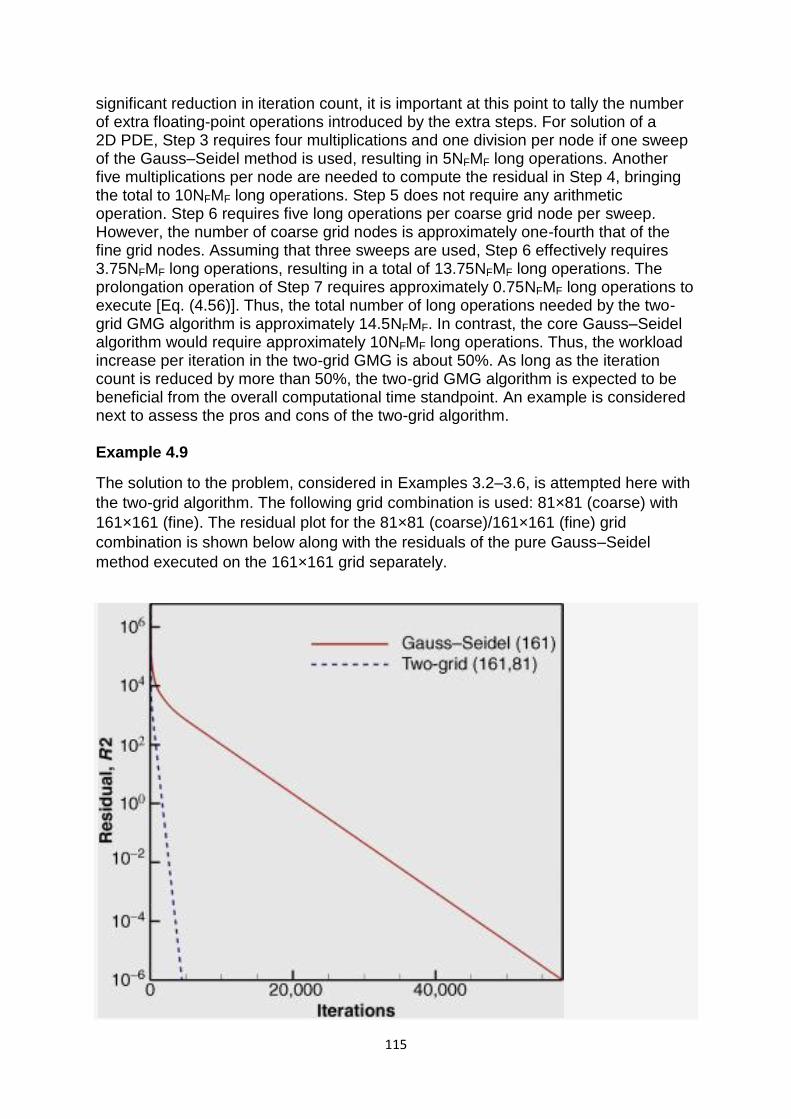
115

significant reduction in iteration count, it is important at this point to tally the number of extra floating-point operations introduced by the extra steps. For solution of a 2D PDE, Step 3 requires four multiplications and one division per node if one sweep of the Gauss–Seidel method is used, resulting in 5NFMF long operations. Another five multiplications per node are needed to compute the residual in Step 4, bringing the total to 10NFMF long operations. Step 5 does not require any arithmetic operation. Step 6 requires five long operations per coarse grid node per sweep. However, the number of coarse grid nodes is approximately one-fourth that of the fine grid nodes. Assuming that three sweeps are used, Step 6 effectively requires 3.75NFMF long operations, resulting in a total of 13.75NFMF long operations. The prolongation operation of Step 7 requires approximately 0.75NFMF long operations to execute [Eq. (4.56)]. Thus, the total number of long operations needed by the two-grid GMG algorithm is approximately 14.5NFMF. In contrast, the core Gauss–Seidel algorithm would require approximately 10NFMF long operations. Thus, the workload increase per iteration in the two-grid GMG is about 50%. As long as the iteration count is reduced by more than 50%, the two-grid GMG algorithm is expected to be beneficial from the overall computational time standpoint. An example is considered next to assess the pros and cons of the two-grid algorithm. Example 4.9

The solution to the problem, considered in Examples 3.2–3.6, is attempted here with

the two-grid algorithm. The following grid combination is used: 81×81 (coarse) with

161×161 (fine). The residual plot for the 81×81 (coarse)/161×161 (fine) grid

combination is shown below along with the residuals of the pure Gauss–Seidel

method executed on the 161×161 grid separately.

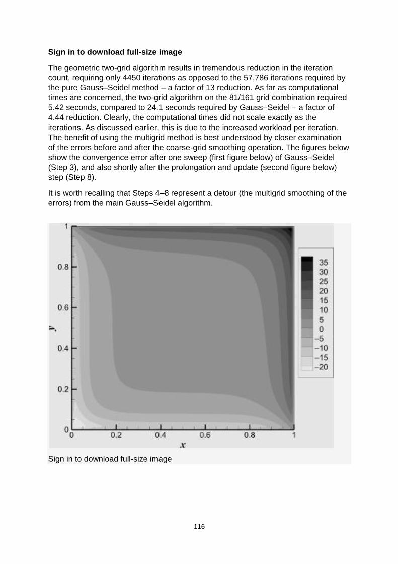
116

Sign in to download full-size image

The geometric two-grid algorithm results in tremendous reduction in the iteration

count, requiring only 4450 iterations as opposed to the 57,786 iterations required by

the pure Gauss–Seidel method – a factor of 13 reduction. As far as computational

times are concerned, the two-grid algorithm on the 81/161 grid combination required

5.42 seconds, compared to 24.1 seconds required by Gauss–Seidel – a factor of

4.44 reduction. Clearly, the computational times did not scale exactly as the

iterations. As discussed earlier, this is due to the increased workload per iteration.

The benefit of using the multigrid method is best understood by closer examination

of the errors before and after the coarse-grid smoothing operation. The figures below

show the convergence error after one sweep (first figure below) of Gauss–Seidel

(Step 3), and also shortly after the prolongation and update (second figure below)

step (Step 8).

It is worth recalling that Steps 4–8 represent a detour (the multigrid smoothing of the

errors) from the main Gauss–Seidel algorithm.

Sign in to download full-size image

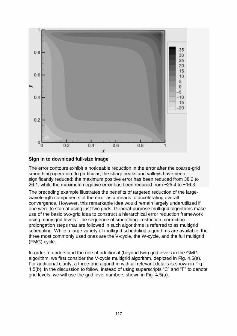
117

Sign in to download full-size image

The error contours exhibit a noticeable reduction in the error after the coarse-grid smoothing operation. In particular, the sharp peaks and valleys have been significantly reduced: the maximum positive error has been reduced from 38.2 to 26.1, while the maximum negative error has been reduced from −25.4 to −16.3.

The preceding example illustrates the benefits of targeted reduction of the large-wavelength components of the error as a means to accelerating overall convergence. However, this remarkable idea would remain largely underutilized if one were to stop at using just two grids. General-purpose multigrid algorithms make use of the basic two-grid idea to construct a hierarchical error reduction framework using many grid levels. The sequence of smoothing–restriction–correction–prolongation steps that are followed in such algorithms is referred to as multigrid scheduling. While a large variety of multigrid scheduling algorithms are available, the three most commonly used ones are the V-cycle, the W-cycle, and the full multigrid (FMG) cycle. In order to understand the role of additional (beyond two) grid levels in the GMG algorithm, we first consider the V-cycle multigrid algorithm, depicted in Fig. 4.5(a). For additional clarity, a three-grid algorithm with all relevant details is shown in Fig. 4.5(b). In the discussion to follow, instead of using superscripts ―C‖ and ―F‖ to denote grid levels, we will use the grid level numbers shown in Fig. 4.5(a).

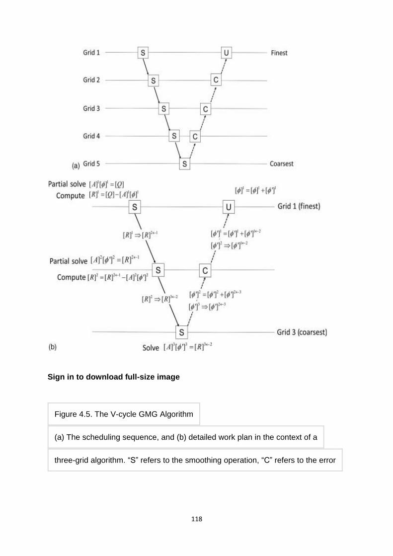
118

Sign in to download full-size image

Figure 4.5. The V-cycle GMG Algorithm

(a) The scheduling sequence, and (b) detailed work plan in the context of a

three-grid algorithm. ―S‖ refers to the smoothing operation, ―C‖ refers to the error

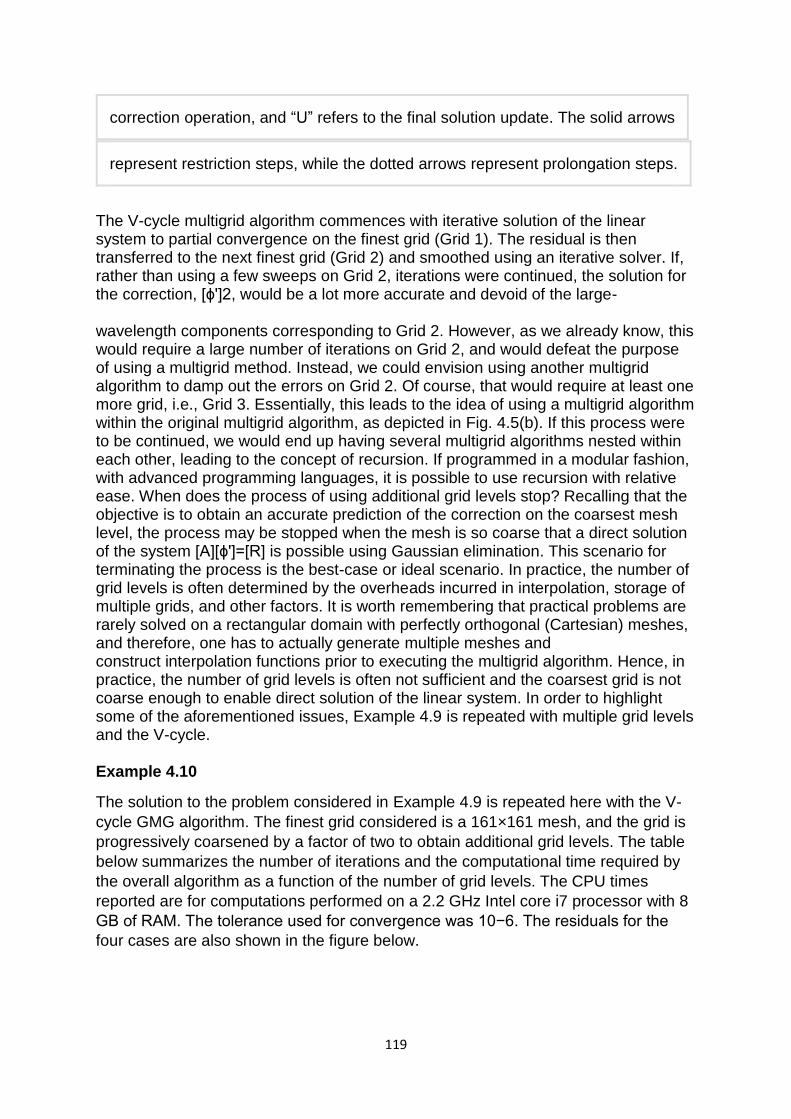
119

correction operation, and ―U‖ refers to the final solution update. The solid arrows

represent restriction steps, while the dotted arrows represent prolongation steps.

The V-cycle multigrid algorithm commences with iterative solution of the linear system to partial convergence on the finest grid (Grid 1). The residual is then transferred to the next finest grid (Grid 2) and smoothed using an iterative solver. If, rather than using a few sweeps on Grid 2, iterations were continued, the solution for the correction, [ϕ']2, would be a lot more accurate and devoid of the large- wavelength components corresponding to Grid 2. However, as we already know, this would require a large number of iterations on Grid 2, and would defeat the purpose of using a multigrid method. Instead, we could envision using another multigrid algorithm to damp out the errors on Grid 2. Of course, that would require at least one more grid, i.e., Grid 3. Essentially, this leads to the idea of using a multigrid algorithm within the original multigrid algorithm, as depicted in Fig. 4.5(b). If this process were to be continued, we would end up having several multigrid algorithms nested within each other, leading to the concept of recursion. If programmed in a modular fashion, with advanced programming languages, it is possible to use recursion with relative ease. When does the process of using additional grid levels stop? Recalling that the objective is to obtain an accurate prediction of the correction on the coarsest mesh level, the process may be stopped when the mesh is so coarse that a direct solution of the system [A][ϕ']=[R] is possible using Gaussian elimination. This scenario for terminating the process is the best-case or ideal scenario. In practice, the number of grid levels is often determined by the overheads incurred in interpolation, storage of multiple grids, and other factors. It is worth remembering that practical problems are rarely solved on a rectangular domain with perfectly orthogonal (Cartesian) meshes, and therefore, one has to actually generate multiple meshes and construct interpolation functions prior to executing the multigrid algorithm. Hence, in practice, the number of grid levels is often not sufficient and the coarsest grid is not coarse enough to enable direct solution of the linear system. In order to highlight some of the aforementioned issues, Example 4.9 is repeated with multiple grid levels and the V-cycle. Example 4.10

The solution to the problem considered in Example 4.9 is repeated here with the V-

cycle GMG algorithm. The finest grid considered is a 161×161 mesh, and the grid is

progressively coarsened by a factor of two to obtain additional grid levels. The table

below summarizes the number of iterations and the computational time required by

the overall algorithm as a function of the number of grid levels. The CPU times

reported are for computations performed on a 2.2 GHz Intel core i7 processor with 8

GB of RAM. The tolerance used for convergence was 10−6. The residuals for the

four cases are also shown in the figure below.

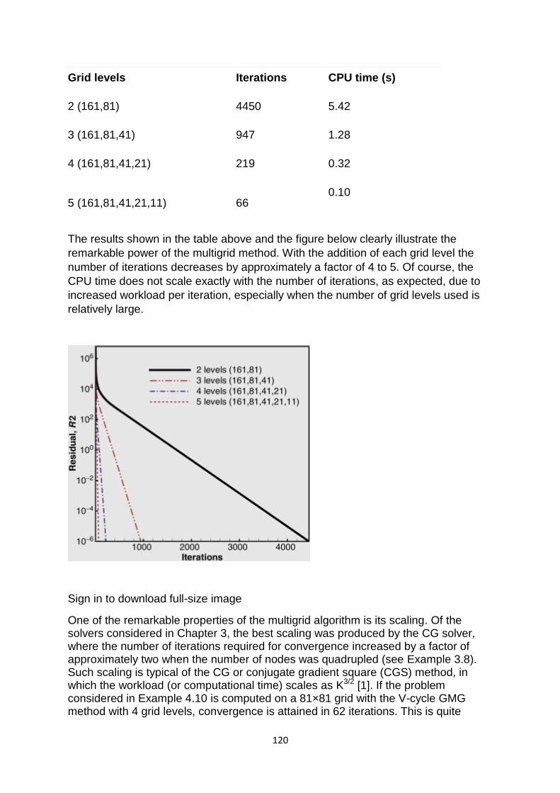
120

Grid levels Iterations CPU time (s)

2 (161,81) 4450 5.42

3 (161,81,41) 947 1.28

4 (161,81,41,21) 219 0.32

5 (161,81,41,21,11) 66 0.10

The results shown in the table above and the figure below clearly illustrate the

remarkable power of the multigrid method. With the addition of each grid level the

number of iterations decreases by approximately a factor of 4 to 5. Of course, the

CPU time does not scale exactly with the number of iterations, as expected, due to

increased workload per iteration, especially when the number of grid levels used is

relatively large.

Sign in to download full-size image

One of the remarkable properties of the multigrid algorithm is its scaling. Of the solvers considered in Chapter 3, the best scaling was produced by the CG solver, where the number of iterations required for convergence increased by a factor of approximately two when the number of nodes was quadrupled (see Example 3.8). Such scaling is typical of the CG or conjugate gradient square (CGS) method, in which the workload (or computational time) scales as K3/2 [1]. If the problem considered in Example 4.10 is computed on a 81×81 grid with the V-cycle GMG method with 4 grid levels, convergence is attained in 62 iterations. This is quite

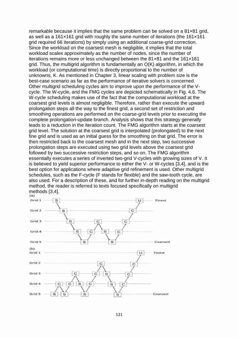
121

remarkable because it implies that the same problem can be solved on a 81×81 grid, as well as a 161×161 grid with roughly the same number of iterations (the 161×161 grid required 66 iterations) by simply using an additional coarse-grid correction. Since the workload on the coarsest mesh is negligible, it implies that the total workload scales approximately as the number of nodes, since the number of iterations remains more or less unchanged between the 81×81 and the 161×161 grid. Thus, the multigrid algorithm is fundamentally an O(K) algorithm, in which the workload (or computational time) is directly proportional to the number of unknowns, K. As mentioned in Chapter 3, linear scaling with problem size is the best-case scenario as far as the performance of iterative solvers is concerned. Other multigrid scheduling cycles aim to improve upon the performance of the V-cycle. The W-cycle, and the FMG cycles are depicted schematically in Fig. 4.6. The W-cycle scheduling makes use of the fact that the computational workload at the coarsest grid levels is almost negligible. Therefore, rather than execute the upward prolongation steps all the way to the finest grid, a second set of restriction and smoothing operations are performed on the coarse-grid levels prior to executing the complete prolongation-update branch. Analysis shows that this strategy generally leads to a reduction in the iteration count. The FMG algorithm starts at the coarsest grid level. The solution at the coarsest grid is interpolated (prolongated) to the next fine grid and is used as an initial guess for the smoothing on that grid. The error is then restricted back to the coarsest mesh and in the next step, two successive prolongation steps are executed using two grid levels above the coarsest grid followed by two successive restriction steps, and so on. The FMG algorithm essentially executes a series of inverted two-grid V-cycles with growing sizes of V. It is believed to yield superior performance to either the V- or W-cycles [3,4], and is the best option for applications where adaptive grid refinement is used. Other multigrid schedules, such as the F-cycle (F stands for flexible) and the saw-tooth cycle, are also used. For a description of these, and for further in-depth reading on the multigrid method, the reader is referred to texts focused specifically on multigrid methods [3,4].

122

Rate of Convergence

In numerical analysis, the speed at which a convergent sequence approaches its limit is called the rate of convergence. Although strictly speaking, a limit does not give information about any finite first part of the sequence, this concept is of practical importance if we deal with a sequence of successive approximations for an iterative method as then typically fewer iterations are needed to yield a useful approximation if the rate of convergence is higher. This may even make the difference between needing ten or a million iterations.Similar concepts are used for discretization methods. The solution of the discretized problem converges to the solution of the continuous problem as the grid size goes to zero, and the speed of convergence is one of the factors of the efficiency of the method. However, the terminology in this case is different from the terminology for iterative methods.

The rate of convergence of an iterative method is represented by mu (μ) and is defined as such:

Suppose the sequence{xn} (generated by an iterative method to find an approximation to a fixed point) converges to a point x, then

limn->[infinity] = |xn+1-x|/|xn-x|[alpha]=μ, where μâ‰≦0 and α(alpha)=order of convergence.

In cases where α=2 or 3 the sequence is said to have quadratic and cubic convergence respectively. However in linear cases i.e. when α=1, for the sequence to converge μ must be in the interval (0,1). The theory behind this is that for En+1≤μEn to converge the absolute errors must decrease with each approximation, and to guarantee this, we have to set 0<μ<1.

In cases where α=1 and μ=1 and you know it converges (since μ=1 does not tell us if it converges or diverges) the sequence {xn} is said to converge sublinearly i.e. the order of convergence is less than one. If μ>1 then the sequence diverges. If μ=0 then it is said to converge superlinearly i.e. it‘s order of convergence is higher than 1, in these cases you change α to a higher value to find what the order of convergence is. In cases where μ is negative, the iteration diverges.

123

UNIT-IV Interpolation and approximation Finite Differences The finite difference method (FDM) is an approximate method for solving partial differential equations. It has been used to solve a wide range of problems. These include linear and non-linear, time independent and dependent problems. This method can be applied to problems with different boundary shapes, different kinds of boundary conditions, and for a region containing a number of different materials. Even though the method was known by such workers as Gauss and Boltzmann, it was not widely used to solve engineering problems until the 1940s. The mathematical basis of the method was already known to Richardson in 1910 [1] and many mathematical books such as references [2 and 3] were published which discussed the finite difference method. Specific reference concerning the treatment of electric and magnetic field problems is made in [4]. The application of FDM is not difficult as it involves only simple arithmetic in the derivation of the discretization equations and in writing the corresponding programs. During 1950–1970 FDM was the most important numerical method used to solve practical problems ([5–7]). With the development of high speed computers having large scale storage capability many numerical solution techniques appeared for solving partial differential equations. However, due to the ease of application of the finite difference method it is still a valuable means of solving these problems

Polynomial interpolation

Here we shall work with polynomials. These are functions with the following

form:f(x)=a0+a1x+⋯+anxn,where n is any nonnegative integer, a0,...,an are any

fixed numbers, with an≠0. Here are some terminology related to polynomials:

1. n is called the degree,

2. a0,...,an are called the coefficients

3. a0 is called the constant term

Polynomials have many uses in mathematics. Here we shall learn about polynomial

interpolation. The following example introduces this.

EXAMPLE: Suppose that f(x) is a polynomial of degree 2 with f(1)=2, f(2)=5, and f(4)=2. Find the formula of f(x).

SOLUTION: Since f(x) has degree 2, it must be of the formf(x)=a+bx+cx2,where the

coefficient a,b,c are to be determined. Since f(1)=2,2=a+b×1+c×12=a+b+c.Similarly,

we get two other equations:5=a+2b+4c2=a+4b+16cSolving all the three equations

together we get a=−4,b=15/2,c=−3/2.

124

In this example we say that f interpolates the three points(1,2),(2,5) and (4,2).We

also call f an interpolating polynomial for this set of 3 points.

Here we see that there is exactly one polynomial of degree 2 that interpolates these

3 points. A polynomial of degree 2 has 2+1=3 unknown coefficients, a,b and c. We

solved for these from the 3 equations. This can be generalized to the following

result.TheoremSuppose that we

have n+1 points:(x0,y0),(x1,y1),...,(xn,yn),where x0,...,xn are distinct numbers (no

such condition on the yi's). Then there is exactly one polynomial f of degree ≤n that

interpolates these n+1 points, i.e.,f(xi)=yi for 0≤i≤n.

Proof: The conditionsf(xi)=yi for 0≤i≤ncan be written as a linear system in terms of the coefficients of the polynomial:Vb=y,where b=(b0,b1,...,bn)′ is the vector of coefficients to be

determined, y=(y0,...,yn) andV=[1x0x20⋯xn01x1x21⋯xn1⋮⋮⋮⋮⋮1xnx2n⋯xnn].One may check by induction that V has determinant|V|=∏i>j(xi−xj).Since the xi's are all distinct, this implies that V is nonsingular, completing the proof. By the way, V is an important matrix that is useful elsewhere also. It is called a Vandermonde matrix. [QED]

In this page we shall learn to solve the following problem:

Given (n+1) points (x0,y0),...,(xn,yn), how to find the unique interpolating

polynomial f(x) with degree ≤n?

We shall always assume that the xi's are distinct. (Why is this a natural assumption?)

One possible way is to imitate the proof of the above theorem, and solve a linear

system of n+1 equations in n+1 unknowns. But this is not efficient, because it fails to

take into account the Vandermonde structure of the coefficient matrix. We shall now

learn some simpler ways of finding f(x).

Lagrange's formula

Lagrange devised a technique by which one may immediately write down the

interpolating polynomial. We shall explore his intuitive approach through a few

examples.

EXAMPLE: Can you quickly write down a nonzero polynomial that vanishes at 1, 3 and 100?

SOLUTION: Typically the simplest answer to flash across our minds,

is (x−1)(x−3)(x−100). You can also multiply this with any other polynomial to get

another answer. Indeed, all answers may be obtained in this way.

Lagrange started with this simple idea, and extended it to the following problem.

EXAMPLE: Same problem as before, but now with the two extra conditions: f must have degree ≤3 and also f(50)=1.

125

SOLUTION: Since we still need f to vanish at 1, 3 and 100, we must start building

from (x−1)(x−3)(x−100). This already has degree 3. So no further growth is allowed.

We can only multiply it with some constant. At x=50 this has

value (50−1)(50−3)(50−100). To bring it down to 1, we have to divide it by this to get

the unique answer:f(x)=(x−1)(x−3)(x−100)(50−1)(50−3)(50−100).

This motivates the definition of Lagrangian polynomial s. If x0,...,xn are

any n+1 distinct numbers, then for i=0,1,...,n, the i-th Lagrangian polynomial is

defined

asLi(x)=(x−x0)×⋯×(x−xi−1)×(x−xi+1)×⋯×(x−xn)(xi−x0)×⋯×(xi−xi−1)×(xi−xi+1)×⋯×(x

−xn).

Here the numerator is the product of all terms of the form (x−xj) for j≠i. The

denominator is the same as the numerator, except that x is replaced by xi.

EXERCISE: Show that Li(x) is the unique ≤n degree polynomial with Li(xi)=1 and Li(xj)=0 for all j≠i.

Let us compute the Li's explicitly in an example.

EXAMPLE: Consider the following xi's: x0=1, x1=3 and x2=−2. Find the Lagrangian polynomials.

SOLUTION: HereL0(x)=(x−3)×(x−(−2))(1−3)×(1−(−2))=(6+x−x2)/6.

Similarly, check thatL1(x)=(x2+x−2)/10,

andL2(x)=(x2−4x+3)/15.

Observe that this example does not mention the yi's at all, since they are not

required to compute the Li's.

Lagrange's interpolationConsider the original problem of

interpolating (x0,y0),...,(xn,yn). The unique interpolating polynomial of degree ≤n is

given byf(x)=y0L0(x)+y1L1(x)+⋯+ynLn(x).

This is called the Lagrangian interpolating polynomial.

Proof: It is easy to see why this f(x) answers our need. At x=xif(xi)=y0L0(xi)+y1L1(xi)+⋯+ynLn(xi)=y0×0+y1×0+⋯+yi×1+⋯+yn×0=yi

[QED]

EXAMPLE: Let us apply Lagrange interpolation to the following table:

i xi yi 0 1 12 1 3 10 2 -2 -15

126

We have already computed the polynomials L0,L1 and L2. So the unique degree 3

interpolating polynomial

isf(x)=y0L0(x)+y1L1(x)+y2L2(x)=12(6+x−x2)/6+10(x2+x−2)/10−15(x2−4x+3)/15=−2x

2+7x+7.

EXERCISE: Find the interpolating polynomial for the following points using Lagrange's method.

i xi yi 0 1 0 1 3 -1 2 -2 3 3 0 100

EXAMPLE: Show thatL0(x)+L1(x)+⋯+Ln(x)=1.

Let f(x) denote the left hand side. Notice that it is the Lagrangian interpolating

polynomial ify0=y1=⋯=yn=1.

Thus f(x) is a polynomial of degree ≤n interpolating the (n+1) points(x0,1),...,(xn,1).

Now consider the constant polynomialg(x)≡1.

It is a polynomial of degree ≤n that interpolates the same (n+1) points.

Since there is exactly one polynomial of degree ≤n interpolating (n+1) given points,

we must havef(x)=g(x),

that is,L0(x)+L1(x)+⋯+Ln(x)=1.

Newton's divided difference method

Lagrange's method is one way to compute the interpolating polynomial for a given

set of points. Here is another method called Newton's divided difference method.

Remember that there is exactly one polynomial of degree ≤n interpolating n+1 given

points. So whether we use Lagrange's method or Newton's method we shall always

come to the same answer. Only the way we compute it will be different, not the final

answer.

As before we are working with the points (x0,y0),...,(xn,yn), where all the xi's are

distinct. We want to find the unique interpolating polynomial, f(x), of degree ≤n. Thus,

we have thatf(xi)=yi for 0≤i≤n.

We define the divided differences of f as follows.

1. 0-th order divided difference:f[x0]=f(x0)

127

2. 1-st order divided difference:f[x1,x0]=f[x1]−f[x0]x1−x0

3. 2-nd order divided difference:f[x2,x1,x0]=f[x2,x1]−f[x1,x0]x2−x0

4. 3-rd order divided difference:f[x3,x2,x1,x0]=f[x3,x2,x1]−f[x2,x1,x0]x3−x0

In general, for 1≤k≤n, we have th k-th order divided

difference:f[xk,xk−1,…,,x1,x0]=f[xk,…,x1]−f[xk−1,…,x0]xk−x0

Notice the following points:

1. The divided differences are computed step by step: the 0-th order divided differences are just the given f(xi)'s. The 1-st order divided differences are computed from the 0-th order divided differences. The 2-nd order is computed from the 1-st order, and so on. This step-by-step computation is best done in a tabular way, as we discuss below.

2. To compute the divided differences we need only the value of f(xi)'s at the given xi's. So even without knowing the formula of f we can compute the divided differences.

3. We are not assuming that the xi's are ordered.

Divided difference table

The following tabular format of the divided differences is called the divided

difference table. Here we have shown it for n=2.

x0 f[x0] f[x1,x0] x1 f[x1] f[x2,x1,x0] f[x2,x1] x2 f[x2] We compute this table starting from the left and proceeding toward right.

EXAMPLE: Consider these values:

xi 0 1 3 4 yi -5 1 25 55 Compute the divided difference table for it.

SOLUTION:

0 -5 6 1 1 2 12 1 3 25 6 30 4 55 For instance, the 6 at the top of the 3rd column is obtained as6=1−(−5)1−0.

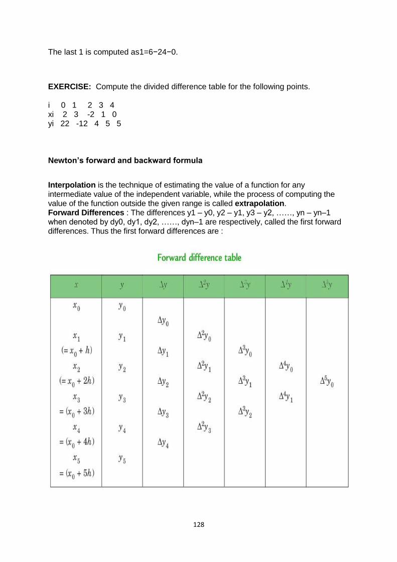
128

The last 1 is computed as1=6−24−0.

EXERCISE: Compute the divided difference table for the following points.

i 0 1 2 3 4 xi 2 3 -2 1 0 yi 22 -12 4 5 5 Newton’s forward and backward formula

Interpolation is the technique of estimating the value of a function for any intermediate value of the independent variable, while the process of computing the value of the function outside the given range is called extrapolation. Forward Differences : The differences y1 – y0, y2 – y1, y3 – y2, ……, yn – yn–1 when denoted by dy0, dy1, dy2, ……, dyn–1 are respectively, called the first forward differences. Thus the first forward differences are :

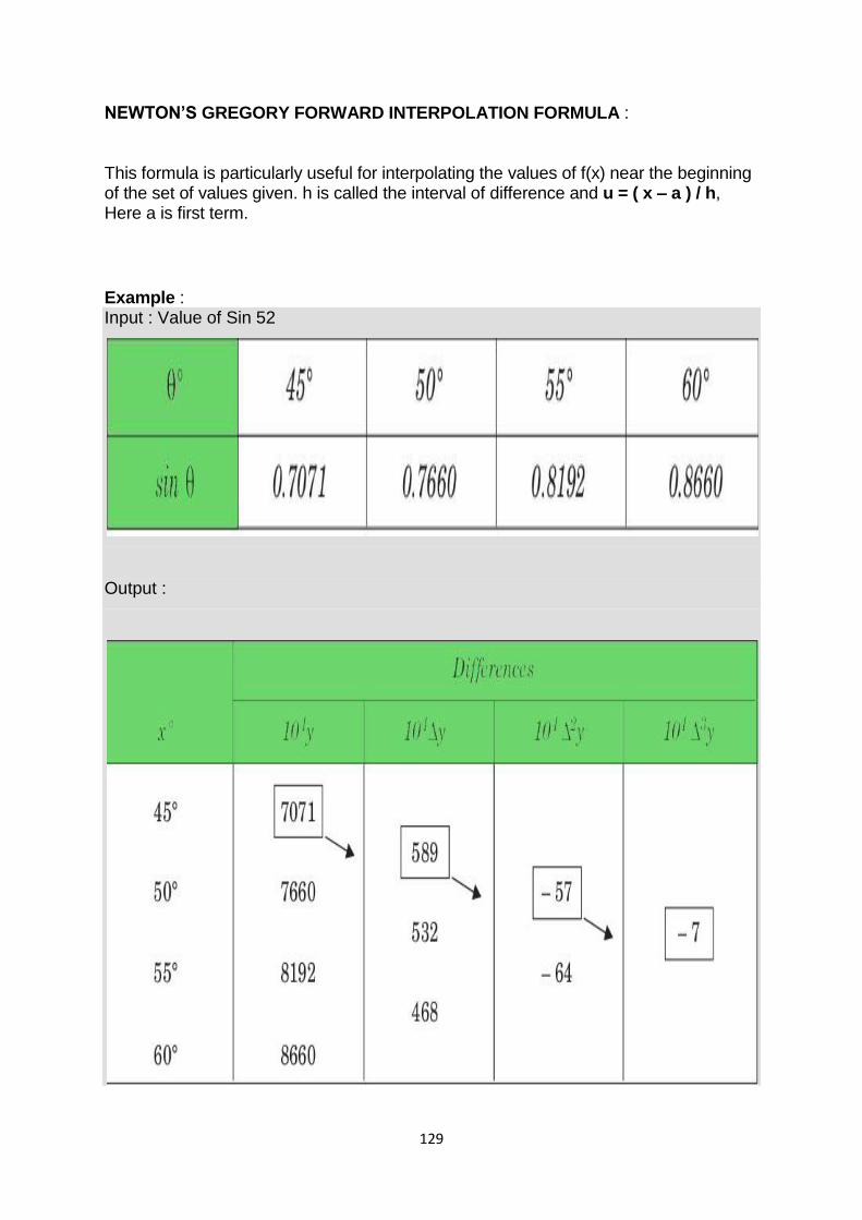
129

NEWTON’S GREGORY FORWARD INTERPOLATION FORMULA :

This formula is particularly useful for interpolating the values of f(x) near the beginning of the set of values given. h is called the interval of difference and u = ( x – a ) / h, Here a is first term.

Example : Input : Value of Sin 52

Output :

130

Value at Sin 52 is 0.788003 Below is the implementation of newton forward interpolation method.

C++

Java

Python3

C#

PHP

filter_none

edit

play_arrow

brightness_4 // CPP Program to interpolate using

// newton forward interpolation

#include <bits/stdc++.h>

usingnamespacestd;

// calculating u mentioned in the formula

floatu_cal(floatu, intn)

{

floattemp = u;

for(inti = 1; i < n; i++)

temp = temp * (u - i);

returntemp;

}

// calculating factorial of given number n

intfact(intn)

{

intf = 1;

for(inti = 2; i <= n; i++)

f *= i;

returnf;

}

131

intmain()

{

// Number of values given

intn = 4;

floatx[] = { 45, 50, 55, 60 };

// y[][] is used for difference table

// with y[][0] used for input

floaty[n][n];

y[0][0] = 0.7071;

y[1][0] = 0.7660;

y[2][0] = 0.8192;

y[3][0] = 0.8660;

// Calculating the forward difference

// table

for(inti = 1; i < n; i++) {

for(intj = 0; j < n - i; j++)

y[j][i] = y[j + 1][i - 1] - y[j][i - 1];

}

// Displaying the forward difference table

for(inti = 0; i < n; i++) {

cout << setw(4) << x[i]

<< "\t";

for(intj = 0; j < n - i; j++)

cout << setw(4) << y[i][j]

<< "\t";

cout << endl;

132

}

// Value to interpolate at

floatvalue = 52;

// initializing u and sum

floatsum = y[0][0];

floatu = (value - x[0]) / (x[1] - x[0]);

for(inti = 1; i < n; i++) {

sum = sum + (u_cal(u, i) * y[0][i]) /

fact(i);

}

cout << "\n Value at "<< value << " is "

<< sum << endl;

return0;

}

Output:

45 0.7071 0.0589 -0.00569999 -0.000699997

50 0.766 0.0532 -0.00639999

55 0.8192 0.0468

60 0.866

Value at 52 is 0.788003

Backward Differences : The differences y1 – y0, y2 – y1, ……, yn – yn–1 when denoted by dy1, dy2, ……, dyn, respectively, are called first backward difference. Thus the first backward differences are :

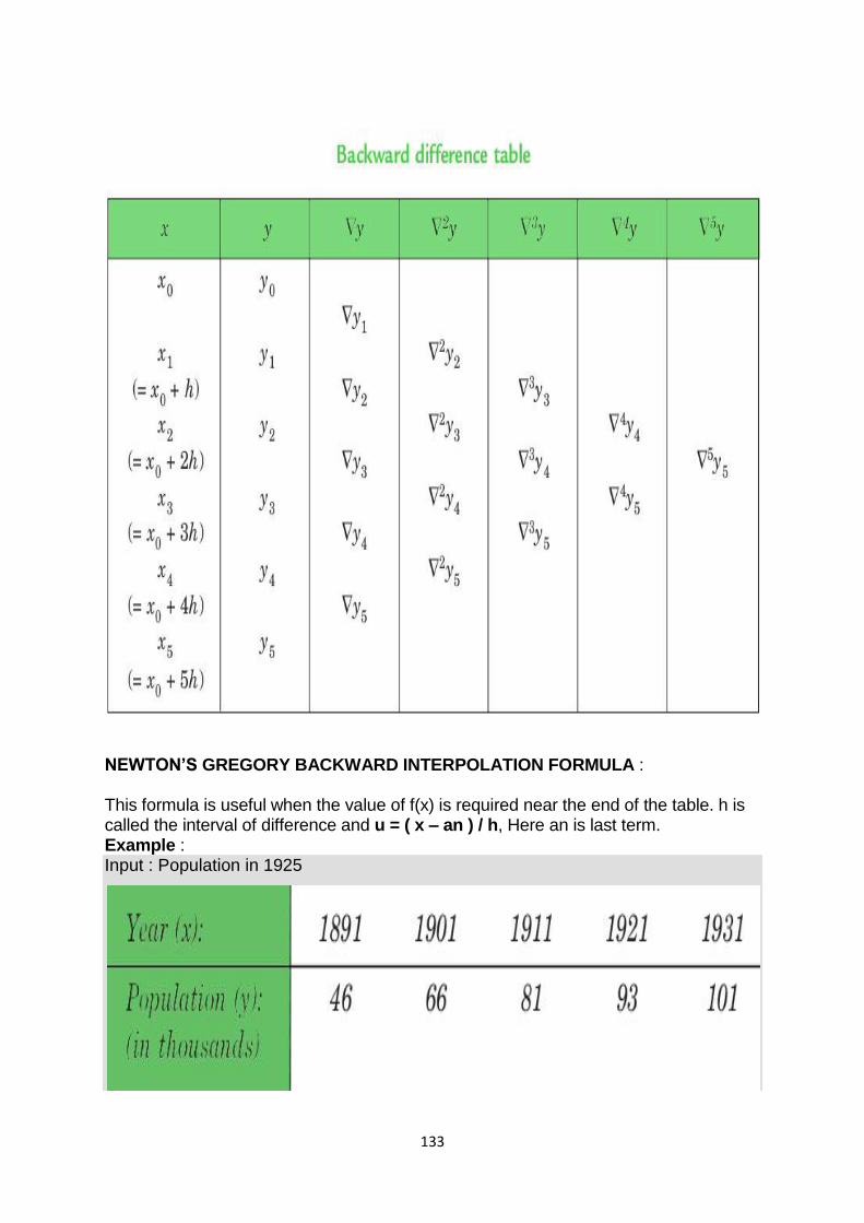
133

NEWTON’S GREGORY BACKWARD INTERPOLATION FORMULA : This formula is useful when the value of f(x) is required near the end of the table. h is called the interval of difference and u = ( x – an ) / h, Here an is last term. Example : Input : Population in 1925

134

Output :

Value in 1925 is 96.8368

Below is the implementation of newton backward interpolation method.

C++

Java

C#

PHP

filter_none

edit

play_arrow

brightness_4 // CPP Program to interpolate using

// newton backward interpolation

#include <bits/stdc++.h>

usingnamespacestd;

// Calculation of u mentioned in formula

floatu_cal(floatu, intn)

{

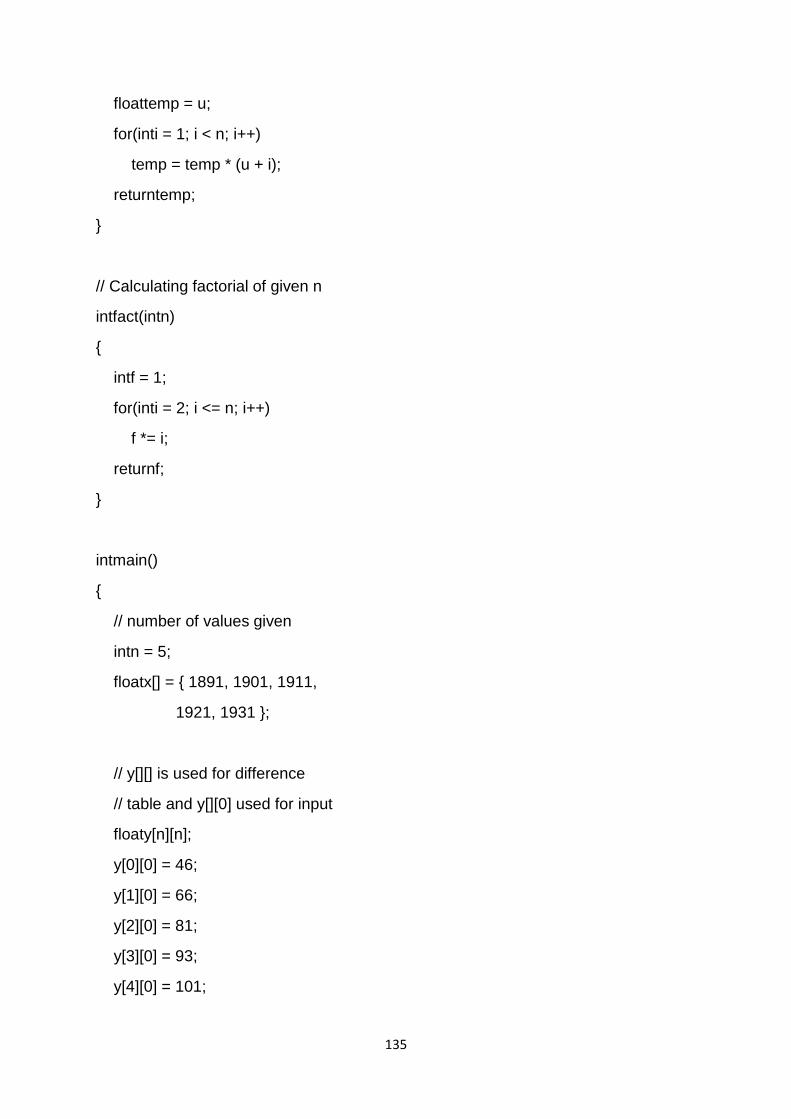
135

floattemp = u;

for(inti = 1; i < n; i++)

temp = temp * (u + i);

returntemp;

}

// Calculating factorial of given n

intfact(intn)

{

intf = 1;

for(inti = 2; i <= n; i++)

f *= i;

returnf;

}

intmain()

{

// number of values given

intn = 5;

floatx[] = { 1891, 1901, 1911,

1921, 1931 };

// y[][] is used for difference

// table and y[][0] used for input

floaty[n][n];

y[0][0] = 46;

y[1][0] = 66;

y[2][0] = 81;

y[3][0] = 93;

y[4][0] = 101;

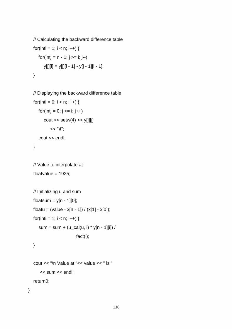
136

// Calculating the backward difference table

for(inti = 1; i < n; i++) {

for(intj = n - 1; j >= i; j--)

y[j][i] = y[j][i - 1] - y[j - 1][i - 1];

}

// Displaying the backward difference table

for(inti = 0; i < n; i++) {

for(intj = 0; j <= i; j++)

cout << setw(4) << y[i][j]

<< "\t";

cout << endl;

}

// Value to interpolate at

floatvalue = 1925;

// Initializing u and sum

floatsum = y[n - 1][0];

floatu = (value - x[n - 1]) / (x[1] - x[0]);

for(inti = 1; i < n; i++) {

sum = sum + (u_cal(u, i) * y[n - 1][i]) /

fact(i);

}

cout << "\n Value at "<< value << " is "

<< sum << endl;

return0;

}

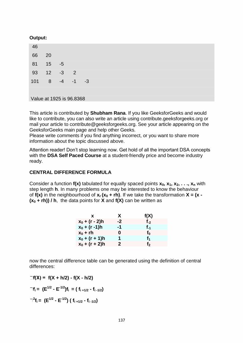
137

Output:

46

66 20

81 15 -5

93 12 -3 2

101 8 -4 -1 -3

Value at 1925 is 96.8368

This article is contributed by Shubham Rana. If you like GeeksforGeeks and would like to contribute, you can also write an article using contribute.geeksforgeeks.org or mail your article to contribute@geeksforgeeks.org. See your article appearing on the GeeksforGeeks main page and help other Geeks. Please write comments if you find anything incorrect, or you want to share more information about the topic discussed above.

Attention reader! Don‘t stop learning now. Get hold of all the important DSA concepts with the DSA Self Paced Course at a student-friendly price and become industry ready. CENTRAL DIFFERENCE FORMULA Consider a function f(x) tabulated for equally spaced points x0, x1, x2, . . ., xn with step length h. In many problems one may be interested to know the behaviour of f(x) in the neighbourhood of xr (x0 + rh). If we take the transformation X = (x - (x0 + rh)) / h, the data points for X and f(X) can be written as

x X f(X) x0 + (r - 2)h -2 f-2 x0 + (r -1)h -1 f-1 x0 + rh 0 f0 x0 + (r + 1)h 1 f1 x0 + (r + 2)h 2 f2

now the central difference table can be generated using the definition of central differences:

f(X + h/2) - f(X - h/2)

i = (E1/2 - E-1/2)fi = ( fi +1/2 - fi -1/2)

2fi = (E1/2 - E-1/2) ( fi +1/2 - fi -1/2)

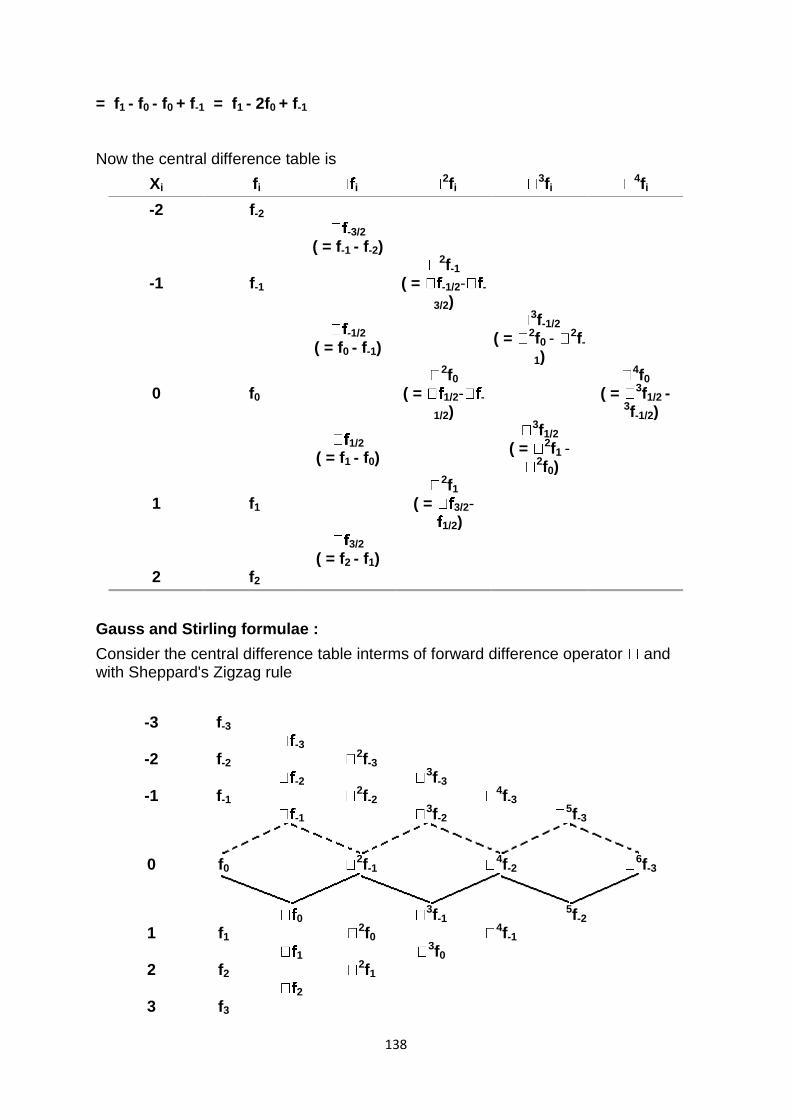
138

= f1 - f0 - f0 + f-1 = f1 - 2f0 + f-1

Now the central difference table is

Xi fi i 2fi

3fi 4fi

-2 f-2

-3/2 ( = f-1 - f-2)

-1 f-1

2f-1 ( = -1/2- -

3/2)

-1/2 ( = f0 - f-1)

3f-1/2 ( = 2f0 -

2f-

1)

0 f0

2f0 ( = 1/2- -

1/2)

4f0 ( = 3f1/2 -

3f-1/2)

1/2 ( = f1 - f0)

3f1/2 ( = 2f1 -

2f0)

1 f1

2f1 ( = 3/2-

1/2)

3/2 ( = f2 - f1)

2 f2

Gauss and Stirling formulae :

Consider the central difference table interms of forward difference operator and with Sheppard's Zigzag rule

-3 f-3 -3

-2 f-2 2f-3 -2 3f-3

-1 f-1 2f-2 4f-3 -1 3f-2 5f-3

0 f0 2f-1 4f-2 6f-3

0 3f-1 5f-2 1 f1 2f0 4f-1

1 3f0 2 f2 2f1

2 3 f3

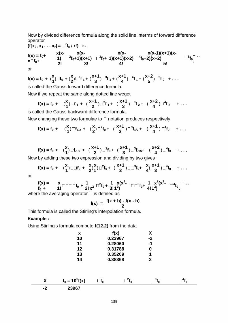
139

Now by divided difference formula along the solid line interms of forward difference operator (f[x0, x1 . . . xr]

= rfx / r!) is

f(x) = f0+

0+

x(x-1) 2f0+

x(x-1)(x+1) 3f0+

x(x-1)(x+1)(x-2) 4f0+

x(x-1)(x+1)(x-2)(x+2) 5f0

+ . . .

2! 3! 4! 5! or

f(x) = f0 + ( x

) 0 + ( x

) 2f-1 + ( x+1

) 3f-1 + ( x+1

) 4f-1 + ( x+2

) 5f-2 + . . . 1 2 3 4 5

is called the Gauss forward difference formula.

Now if we repeat the same along dotted line weget

f(x) = f0 + ( x

) -1 + ( x+1

) 2f-1 + ( x+1

) 3f-2 + ( x+2

) 4f-2 + . . . 1 2 3 4

is called the Gauss backward difference formula.

Now changing these two formulae to notation produces respectively

f(x) = f0 + ( x

) 1/2 + ( x

) 2f0 + ( x+1

) 3f1/2 + ( x+1

) 4f0 + . . . 1 2 3 4

f(x) = f0 + ( x

) -1/2 + ( x+1

) 2f0 + ( x+1

) 3f-1/2+ ( x+2

) 4f0 + . . . 1 2 3 4

Now by adding these two expression and dividing by two gives

f(x) = f0 + ( x

) 0 + x

( x

) 2f0 + ( x+1

) 3f0+ x

( x+1

) 4f0 + . . . 1 2 1 3 4 3

or

f(x) = f0 +

x 0 +

1 x2

2f0 + 1 x(x2-

12) 3f0+

1 x2(x2-12)

4f0 + . . . 1! 2! 3! 4!

where the averaging operator is defined as

= f(x + h) - f(x - h)

2 This formula is called the Stirling's interpolation formula.

Example :

Using Stirling's formula compute f(12.2) from the data

x f(x) X 10 0.23967 -2 11 0.28060 -1 12 0.31788 0 13 0.35209 1 14 0.38368 2

X fx = 105f(x) x 2fx

3fx 4fx

-2 23967

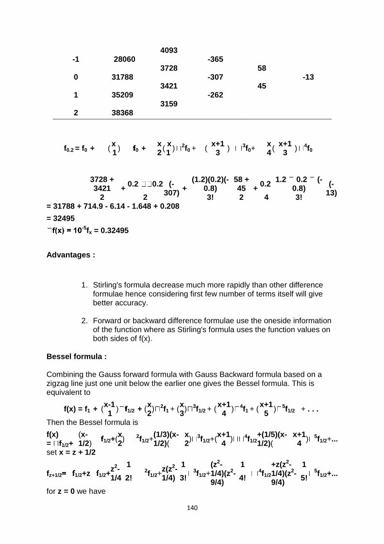
140

4093 -1 28060 -365 3728 58 0 31788 -307 -13 3421 45 1 35209 -262 3159 2 38368

f0.2 = f0 + ( x

) 0 + x

( x

) 2f0 + ( x+1

) 3f0+ x

( x+1

) 4f0 1 2 1 3 4 3

3728 + 3421 +

0.2 0.2 (-307)

+ (1.2)(0.2)(-

0.8) 58 + 45 +

0.2 1.2 0.2 (-

0.8) (-

13) 2 2 3! 2 4 3!

= 31788 + 714.9 - 6.14 - 1.648 + 0.208

= 32495 -5fx = 0.32495

Advantages :

1. Stirling's formula decrease much more rapidly than other difference formulae hence considering first few number of terms itself will give better accuracy.

2. Forward or backward difference formulae use the oneside information of the function where as Stirling's formula uses the function values on both sides of f(x).

Bessel formula :

Combining the Gauss forward formula with Gauss Backward formula based on a zigzag line just one unit below the earlier one gives the Bessel formula. This is equivalent to

f(x) = f1 + ( x-1

) 1/2 + ( x

) 2f1 + ( x

) 3f1/2 + ( x+1

) 4f1 + ( x+1

) 5f1/2 + . . . 1 2 3 4 5

Then the Bessel formula is

f(x) = 1/2+

(x-1/2) 1/2+ (

x ) 2f1/2+

(1/3)(x-1/2)(

x ) 3f1/2+ (

x+1 ) 4f1/2

+(1/5)(x-1/2)(

x+1 ) 5f1/2 +...

2 2 4 4 set x = z + 1/2

fz+1/2 1/2+ z 1/2+ z2-1/4

1 2f1/2+

z(z2-1/4)

1 3f1/2+

(z2-1/4)(z2-9/4)

1 4f1/2

+z(z2-1/4)(z2-9/4)

1 5f1/2 +...

2! 3! 4! 5!

for z = 0 we have

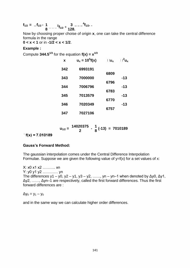
141

f1/2 = 1/2 -

1 2f1/2 + 3 4f1/2. .

. 8 128 Now by choosing proper choise of origin x, one can take the central difference formula in the range 0 < x < 1 or in -1/2 < x < 1/2.

Example :

Compute 344.51/3 for the equation f(x) = x1/3

x ux = 105f(x) x 2ux

342 6993191 6809

343 7000000 -13 6796

344 7006796 -13 6783

345 7013579 -13 6770

346 7020349 -13 6757

347 7027106

u1/2 = 14020375

- 1

(-13) = 7010189 2 8

Gauss’s Forward Method: The gaussian interpolation comes under the Central Difference Interpolation Formulae. Suppose we are given the following value of y=f(x) for a set values of x: X: x0 x1 x2 ………. xn Y: y0 y1 y2 ………… yn The differences y1 – y0, y2 – y1, y3 – y2, ……, yn – yn–1 when denoted by Δy0, Δy1, Δy2, ……, Δyn–1 are respectively, called the first forward differences. Thus the first forward differences are : Δy0 = y1 – y0 and in the same way we can calculate higher order differences.

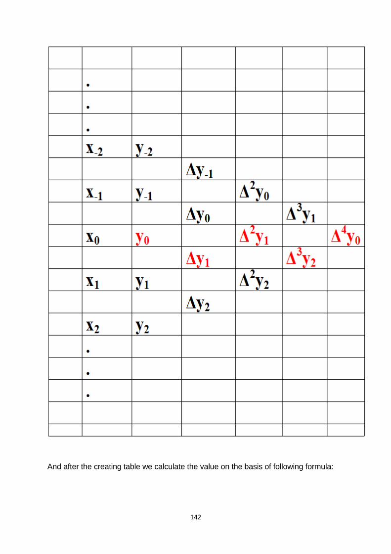
142

And after the creating table we calculate the value on the basis of following formula:

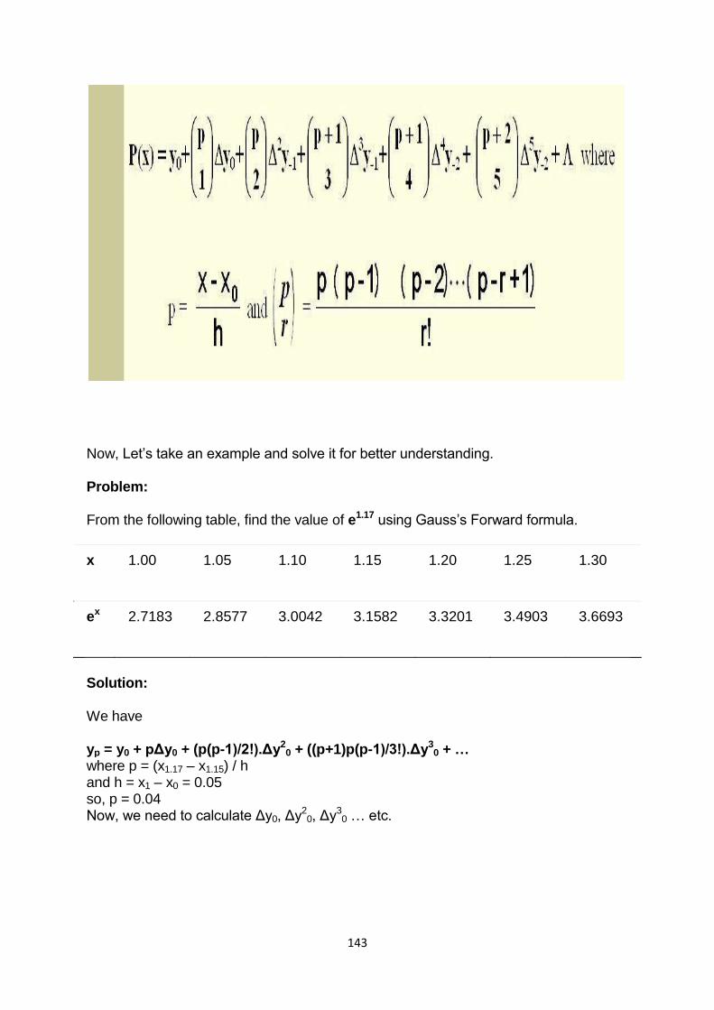
143

Now, Let‘s take an example and solve it for better understanding. Problem: From the following table, find the value of e1.17 using Gauss‘s Forward formula.

x 1.00 1.05 1.10 1.15 1.20 1.25 1.30

ex 2.7183 2.8577 3.0042 3.1582 3.3201 3.4903 3.6693

Solution: We have yp = y0 + pΔy0 + (p(p-1)/2!).Δy2

0 + ((p+1)p(p-1)/3!).Δy30 + …

where p = (x1.17 – x1.15) / h and h = x1 – x0 = 0.05 so, p = 0.04 Now, we need to calculate Δy0, Δy2

0, Δy30 … etc.

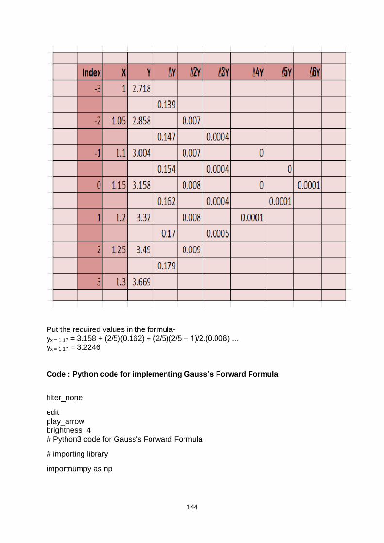
144

Put the required values in the formula- yx = 1.17 = 3.158 + (2/5)(0.162) + (2/5)(2/5 – 1)/2.(0.008) … yx = 1.17 = 3.2246 Code : Python code for implementing Gauss’s Forward Formula

filter_none

edit play_arrow brightness_4 # Python3 code for Gauss's Forward Formula

# importing library

importnumpy as np

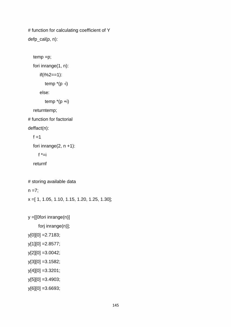
145

# function for calculating coefficient of Y

defp_cal(p, n):

temp =p;

fori inrange(1, n):

if(i%2==1):

temp *(p -i)

else:

temp *(p +i)

returntemp;

# function for factorial

deffact(n):

f =1

fori inrange(2, n +1):

f *=i

returnf

# storing available data

n =7;

x =[ 1, 1.05, 1.10, 1.15, 1.20, 1.25, 1.30];

y =[[0fori inrange(n)]

forj inrange(n)];

y[0][0] =2.7183;

y[1][0] =2.8577;

y[2][0] =3.0042;

y[3][0] =3.1582;

y[4][0] =3.3201;

y[5][0] =3.4903;

y[6][0] =3.6693;

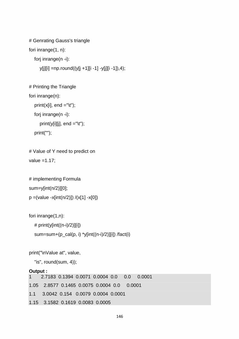
146

# Genrating Gauss's triangle

fori inrange(1, n):

forj inrange(n -i):

y[j][i] =np.round((y[j +1][i -1] -y[j][i -1]),4);

# Printing the Triangle

fori inrange(n):

print(x[i], end ="\t");

forj inrange(n -i):

print(y[i][j], end ="\t");

print("");

# Value of Y need to predict on

value =1.17;

# implementing Formula

sum=y[int(n/2)][0];

p =(value -x[int(n/2)]) /(x[1] -x[0])

fori inrange(1,n):

# print(y[int((n-i)/2)][i])

sum=sum+(p_cal(p, i) *y[int((n-i)/2)][i]) /fact(i)

print("\nValue at", value,

"is", round(sum, 4));

Output : 1 2.7183 0.1394 0.0071 0.0004 0.0 0.0 0.0001

1.05 2.8577 0.1465 0.0075 0.0004 0.0 0.0001

1.1 3.0042 0.154 0.0079 0.0004 0.0001

1.15 3.1582 0.1619 0.0083 0.0005

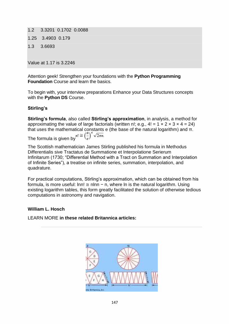
147

1.2 3.3201 0.1702 0.0088

1.25 3.4903 0.179

1.3 3.6693

Value at 1.17 is 3.2246

Attention geek! Strengthen your foundations with the Python Programming Foundation Course and learn the basics. To begin with, your interview preparations Enhance your Data Structures concepts with the Python DS Course. Stirling’s Stirling’s formula, also called Stirling’s approximation, in analysis, a method for approximating the value of large factorials (written n!; e.g., 4! = 1 × 2 × 3 × 4 = 24) that uses the mathematical constants e (the base of the natural logarithm) and π.

The formula is given by

The Scottish mathematician James Stirling published his formula in Methodus Differentialis sive Tractatus de Summatione et Interpolatione Serierum Infinitarum (1730; ―Differential Method with a Tract on Summation and Interpolation of Infinite Series‖), a treatise on infinite series, summation, interpolation, and quadrature.

For practical computations, Stirling‘s approximation, which can be obtained from his

formula, is more useful: lnn! ≅ nlnn − n, where ln is the natural logarithm. Using existing logarithm tables, this form greatly facilitated the solution of otherwise tedious computations in astronomy and navigation.

William L. Hosch

LEARN MORE in these related Britannica articles:

148

analysis

Analysis, a branch of mathematics that deals with continuous change and with

certain general types of processes that have emerged from the study of continuous

change, such as limits, differentiation, and integration. Since the discovery of the

differential and integral calculus by Isaac Newton and Gottfried Wilhelm Leibniz at

the…

factorial

Factorial, in mathematics, the product of all positive integers less than or equal to a

given positive integer and denoted by that integer and an exclamation point. Thus,

factorial seven is written 7!, meaning 1 × 2 × 3 × 4 × 5 × 6 × 7. Factorial zero is…

Bessel functions, first defined by the mathematician Daniel Bernoulli and then

generalized by Friedrich Bessel, are canonical solutions y(x) of Bessel's differential

equation

{\displaystyle x^{2}{\frac {d^{2}y}{dx^{2}}}+x{\frac {dy}{dx}}+\left(x^{2}-\alpha

^{2}\right)y=0}for an arbitrary complex number α, the order of the Bessel function.

Although α and −α produce the same differential equation, it is conventional to define

different Bessel functions for these two values in such a way that the Bessel

functions are mostly smooth functions of α.

The most important cases are when α is an integer or half-integer. Bessel functions

for integer α are also known as cylinder functions or the cylindrical

harmonics because they appear in the solution to Laplace's equation in cylindrical

coordinates. Spherical Bessel functions with half-integer α are obtained when

the Helmholtz equation is solved in spherical coordinates.

Bessel functions of the first kind: Jα

Bessel functions of the first kind, denoted as Jα(x), are solutions of Bessel's differential equation that are finite at the origin (x = 0) for integer or positive α and diverge as x approaches zero for negative non-integer α. It is possible to define the function by its series expansion around x = 0, which can be found by applying the Frobenius method to Bessel's equation:[3]

where Γ(z) is the gamma function, a shifted generalization of the factorial function to non-integer values. The Bessel function of the first kind is an entire function if α is an integer, otherwise it is a multivalued function with singularity at zero. The graphs of Bessel functions look roughly like oscillating sine or cosine functions that decay proportionally to (see also their asymptotic forms below), although their roots are not generally periodic, except asymptotically for large x. (The series indicates that −J1(x) is the derivative of J0(x), much like −sin x is the derivative of cos x; more

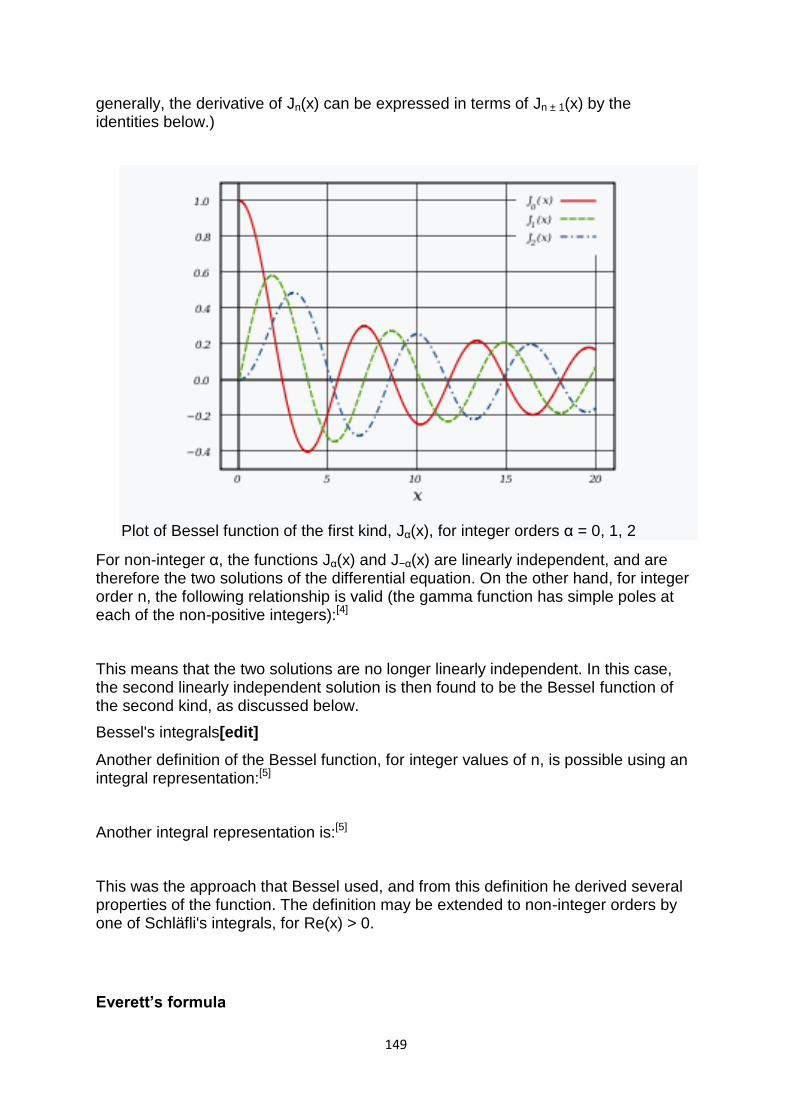
149

generally, the derivative of Jn(x) can be expressed in terms of Jn ± 1(x) by the identities below.)

Plot of Bessel function of the first kind, Jα(x), for integer orders α = 0, 1, 2

For non-integer α, the functions Jα(x) and J−α(x) are linearly independent, and are therefore the two solutions of the differential equation. On the other hand, for integer order n, the following relationship is valid (the gamma function has simple poles at each of the non-positive integers):[4]

This means that the two solutions are no longer linearly independent. In this case, the second linearly independent solution is then found to be the Bessel function of the second kind, as discussed below.

Bessel's integrals[edit]

Another definition of the Bessel function, for integer values of n, is possible using an integral representation:[5]

Another integral representation is:[5]

This was the approach that Bessel used, and from this definition he derived several properties of the function. The definition may be extended to non-integer orders by one of Schläfli's integrals, for Re(x) > 0.

Everett’s formula

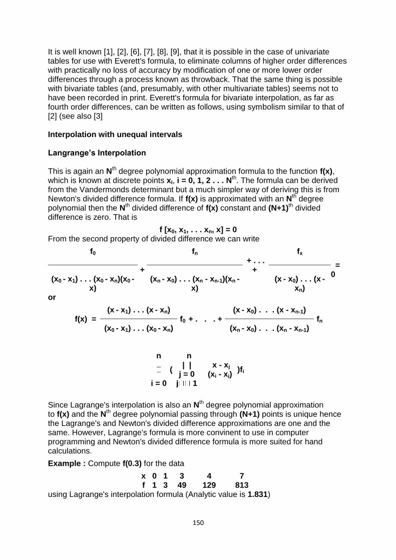
150

It is well known [1], [2], [6], [7], [8], [9], that it is possible in the case of univariate tables for use with Everett's formula, to eliminate columns of higher order differences with practically no loss of accuracy by modification of one or more lower order differences through a process known as throwback. That the same thing is possible with bivariate tables (and, presumably, with other multivariate tables) seems not to have been recorded in print. Everett's formula for bivariate interpolation, as far as fourth order differences, can be written as follows, using symbolism similar to that of [2] (see also [3] Interpolation with unequal intervals Langrange’s Interpolation This is again an Nth degree polynomial approximation formula to the function f(x), which is known at discrete points xi, i = 0, 1, 2 . . . Nth. The formula can be derived from the Vandermonds determinant but a much simpler way of deriving this is from Newton's divided difference formula. If f(x) is approximated with an Nth degree polynomial then the Nth divided difference of f(x) constant and (N+1)th divided difference is zero. That is

f [x0, x1, . . . xn, x] = 0 From the second property of divided difference we can write

f0

+

fn

fx

= 0

+ . . . +

(x0 - x1) . . . (x0 - xn)(x0 - x)

(xn - x0) . . . (xn - xn-1)(xn - x)

(x - x0) . . . (x -

xn) or

(x - x1) . . . (x - xn) (x - x0) . . . (x - xn-1) f(x) = f0 + . . . + fn (x0 - x1) . . . (x0 - xn) (xn - x0) . . . (xn - xn-1)

n

(

n

)fi

| | x - xj

j = 0 (xi - xj) i = 0 1

Since Lagrange's interpolation is also an Nth degree polynomial approximation to f(x) and the Nth degree polynomial passing through (N+1) points is unique hence the Lagrange's and Newton's divided difference approximations are one and the same. However, Lagrange's formula is more convinent to use in computer programming and Newton's divided difference formula is more suited for hand calculations.

Example : Compute f(0.3) for the data

x 0 1 3 4 7 f 1 3 49 129 813

using Lagrange's interpolation formula (Analytic value is 1.831)

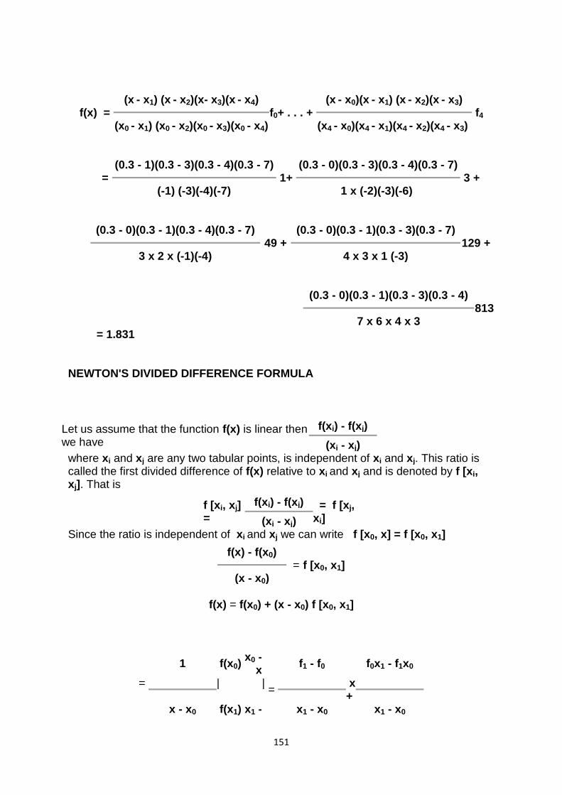
151

(x - x1) (x - x2)(x- x3)(x - x4) (x - x0)(x - x1) (x - x2)(x - x3) f(x) = f0+ . . . + f4 (x0 - x1) (x0 - x2)(x0 - x3)(x0 - x4) (x4 - x0)(x4 - x1)(x4 - x2)(x4 - x3)

(0.3 - 1)(0.3 - 3)(0.3 - 4)(0.3 - 7) (0.3 - 0)(0.3 - 3)(0.3 - 4)(0.3 - 7) = 1+ 3 + (-1) (-3)(-4)(-7) 1 x (-2)(-3)(-6)

(0.3 - 0)(0.3 - 1)(0.3 - 4)(0.3 - 7) (0.3 - 0)(0.3 - 1)(0.3 - 3)(0.3 - 7) 49 + 129 +

3 x 2 x (-1)(-4) 4 x 3 x 1 (-3)

(0.3 - 0)(0.3 - 1)(0.3 - 3)(0.3 - 4) 813

7 x 6 x 4 x 3 = 1.831

NEWTON'S DIVIDED DIFFERENCE FORMULA

Let us assume that the function f(x) is linear then we have

f(xi) - f(xj)

(xi - xj) where xi and xj are any two tabular points, is independent of xi and xj. This ratio is called the first divided difference of f(x) relative to xi and xj and is denoted by f [xi, xj]. That is

f [xi, xj] =

f(xi) - f(xj) = f [xj, xi]

(xi - xj) Since the ratio is independent of xi and xj we can write f [x0, x] = f [x0, x1]

f(x) - f(x0)

= f [x0, x1] (x - x0)

f(x) = f(x0) + (x - x0) f [x0, x1]

=

1

|

f(x0) x0 -

x |

f1 - f0 f0x1 - f1x0

=

x +

x - x0 f(x1) x1 - x1 - x0

x1 - x0

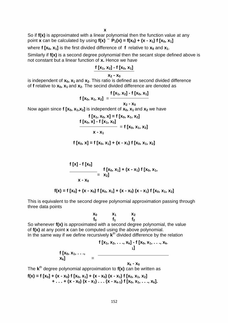
152

x So if f(x) is approximated with a linear polynomial then the function value at any point x can be calculated by using f(x) P1(x) = f(x0) + (x - x1) f [x0, x1]

where f [x0, x1] is the first divided difference of f relative to x0 and x1.

Similarly if f(x) is a second degree polynomial then the secant slope defined above is not constant but a linear function of x. Hence we have

f [x1, x2] - f [x0, x1]

x2 - x0 is independent of x0, x1 and x2. This ratio is defined as second divided difference of f relative to x0, x1 and x2. The secind divided difference are denoted as

f [x1, x2] - f [x0, x1]

f [x0, x1, x2] =

x2 - x0 Now again since f [x0, x1,x2] is independent of x0, x1 and x2 we have

f [x1, x0, x] = f [x0, x1, x2] f [x0, x] - f [x1, x0]

= f [x0, x1, x2]

x - x1

f [x0, x] = f [x0, x1] + (x - x1) f [x0, x1, x2]

f [x] - f [x0]

=

f [x0, x1] + (x - x1) f [x0, x1, x2]

x - x0

f(x) = f [x0] + (x - x0) f [x0, x1] + (x - x0) (x - x1) f [x0, x1, x2]

This is equivalent to the second degree polynomial approximation passing through three data points

x0 x1 x2 f0 f1 f2

So whenever f(x) is approximated with a second degree polynomial, the value of f(x) at any point x can be computed using the above polynomial. In the same way if we define recursively kth divided difference by the relation

f [x1, x2, . . ., xk] - f [x0, x1, . . ., xk-

1] f [x0, x1, . . ., xk]

=

xk - x0 The kth degree polynomial approximation to f(x) can be written as

f(x) = f [x0] + (x - x0) f [x0, x1] + (x - x0) (x - x1) f [x0, x1, x2] + . . . + (x - x0) (x - x1) . . . (x - xk-1) f [x0, x1, . . ., xk].

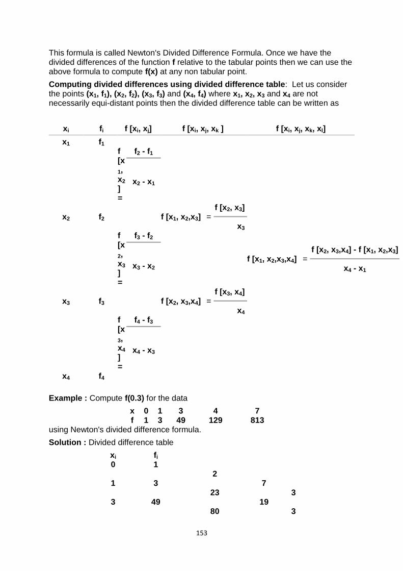
153

This formula is called Newton's Divided Difference Formula. Once we have the divided differences of the function f relative to the tabular points then we can use the above formula to compute f(x) at any non tabular point.

Computing divided differences using divided difference table: Let us consider the points (x1, f1), (x2, f2), (x3, f3) and (x4, f4) where x1, x2, x3 and x4 are not necessarily equi-distant points then the divided difference table can be written as

xi fi f [xi, xj] f [xi, xj, xk ] f [xi, xj, xk, xl]

x1 f1

f [x

1, x2

] =

f2 - f1

x2 - x1

x2 f2

f [x2, x3] - f [x1, x2] f [x1, x2,x3] =

x3 - x1

f [x

2, x3

] =

f3 - f2

x3 - x2

f [x2, x3,x4] - f [x1, x2,x3] f [x1, x2,x3,x4] =

x4 - x1

x3 f3

f [x3, x4] - f [x2, x3] f [x2, x3,x4] =

x4 - x2

f [x

3, x4

] =

f4 - f3

x4 - x3

x4 f4

Example : Compute f(0.3) for the data

x 0 1 3 4 7 f 1 3 49 129 813

using Newton's divided difference formula.

Solution : Divided difference table

xi fi 0 1

2 1 3 7

23 3 3 49 19

80 3

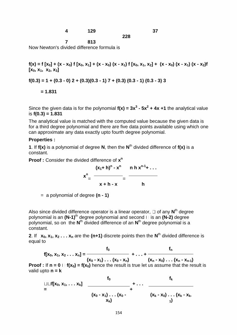
154

4 129 37 228

7 813

Now Newton's divided difference formula is

f(x) = f [x0] + (x - x0) f [x0, x1] + (x - x0) (x - x1) f [x0, x1, x2] + (x - x0) (x - x1) (x - x2)f [x0, x1, x2, x3]

f(0.3) = 1 + (0.3 - 0) 2 + (0.3)(0.3 - 1) 7 + (0.3) (0.3 - 1) (0.3 - 3) 3

= 1.831

Since the given data is for the polynomial f(x) = 3x3 - 5x2 + 4x +1 the analytical value is f(0.3) = 1.831

The analytical value is matched with the computed value because the given data is for a third degree polynomial and there are five data points available using which one can approximate any data exactly upto fourth degree polynomial.

Properties :

1. If f(x) is a polynomial of degree N, then the Nth divided difference of f(x) is a constant.

Proof : Consider the divided difference of xn

(x1+ h)n - xn

n h xn-1+ . . .

n =

=

x + h - x

h

= a polynomial of degree (n - 1)

Also since divided difference operator is a linear operator, of any Nth degree polynomial is an (N-1)th degree polynomial and second is an (N-2) degree polynomial, so on the Nth divided difference of an Nth degree polynomial is a constant.

2. If x0, x1, x2 . . . xn are the (n+1) discrete points then the Nth divided difference is equal to

f0

fn f[x0, x1, x2 . . . xn] = + . . . +

(x0 - x1) . . . (x0 - xn)

(xn - x0) . . . (xn - xn-1)

Proof : If n = 0 f(x0) = f(x0) hence the result is true let us assume that the result is valid upto n = k

f0

fk f[x0, x1, . . . xk]

=

+ . . . +

(x0 - x1) . . . (x0 -

xk) (xk - x0) . . . (xk - xk-

1)

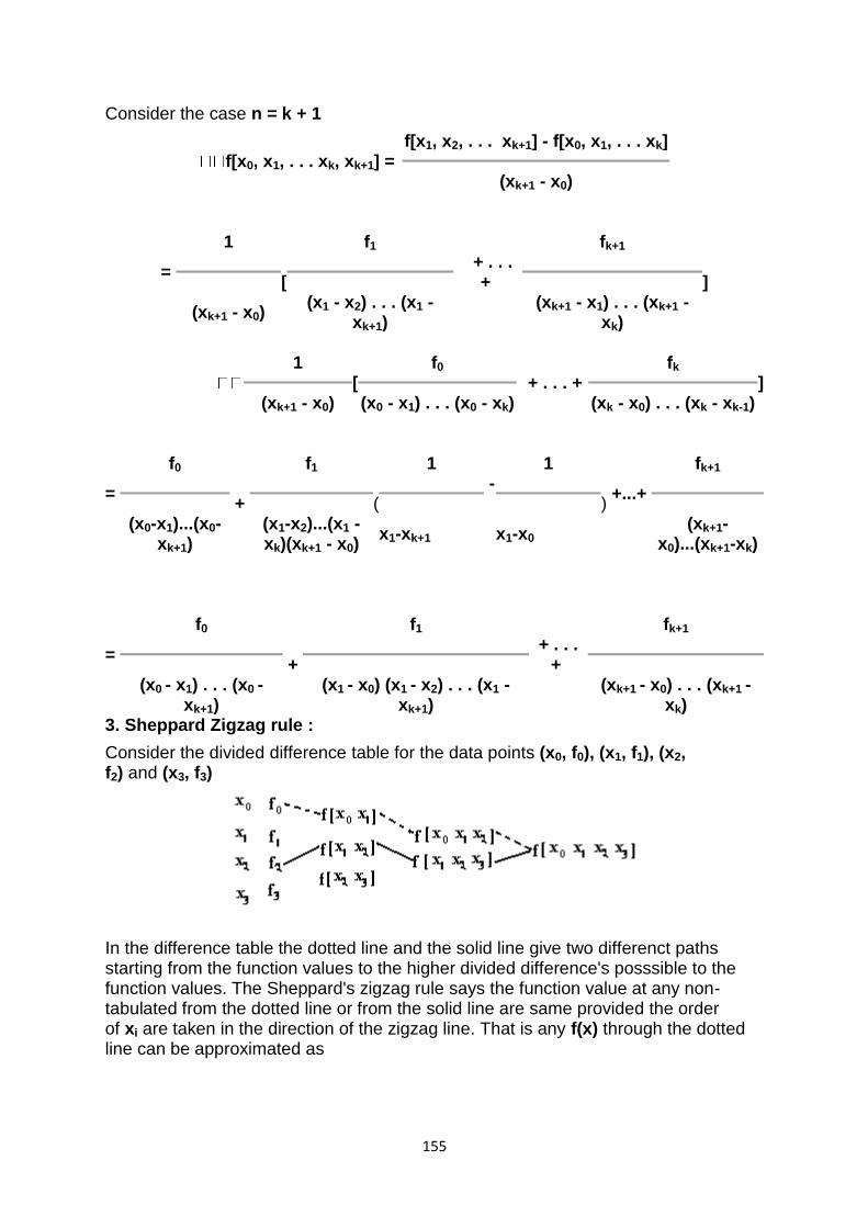
155

Consider the case n = k + 1

f[x1, x2, . . . xk+1] - f[x0, x1, . . . xk]

f[x0, x1, . . . xk, xk+1] =

(xk+1 - x0)

1

[

f1 fk+1

] =

+ . . . +

(xk+1 - x0) (x1 - x2) . . . (x1 -

xk+1)

(xk+1 - x1) . . . (xk+1 - xk)

1

[ f0 fk

] + . . . +

(xk+1 - x0) (x0 - x1) . . . (x0 - xk) (xk - x0) . . . (xk - xk-1) f0

+

f1

(

1

1

)

fk+1

=

-

+...+

(x0-x1)...(x0-

xk+1) (x1-x2)...(x1 - xk)(xk+1 - x0)

x1-xk+1 x1-x0

(xk+1-x0)...(xk+1-xk)

f0

+

f1 fk+1

=

+ . . . +

(x0 - x1) . . . (x0 -

xk+1) (x1 - x0) (x1 - x2) . . . (x1 -

xk+1)

(xk+1 - x0) . . . (xk+1 - xk)

3. Sheppard Zigzag rule :

Consider the divided difference table for the data points (x0, f0), (x1, f1), (x2, f2) and (x3, f3)

In the difference table the dotted line and the solid line give two differenct paths starting from the function values to the higher divided difference's posssible to the function values. The Sheppard's zigzag rule says the function value at any non-tabulated from the dotted line or from the solid line are same provided the order of xi are taken in the direction of the zigzag line. That is any f(x) through the dotted line can be approximated as

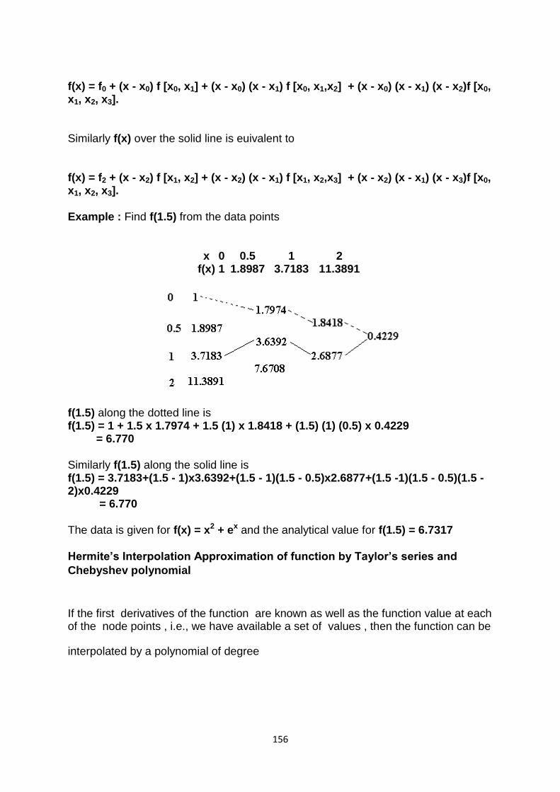
156

f(x) = f0 + (x - x0) f [x0, x1] + (x - x0) (x - x1) f [x0, x1,x2] + (x - x0) (x - x1) (x - x2)f [x0, x1, x2, x3].

Similarly f(x) over the solid line is euivalent to

f(x) = f2 + (x - x2) f [x1, x2] + (x - x2) (x - x1) f [x1, x2,x3] + (x - x2) (x - x1) (x - x3)f [x0, x1, x2, x3].

Example : Find f(1.5) from the data points

x 0 0.5 1 2 f(x) 1 1.8987 3.7183 11.3891

f(1.5) along the dotted line is f(1.5) = 1 + 1.5 x 1.7974 + 1.5 (1) x 1.8418 + (1.5) (1) (0.5) x 0.4229 = 6.770

Similarly f(1.5) along the solid line is f(1.5) = 3.7183+(1.5 - 1)x3.6392+(1.5 - 1)(1.5 - 0.5)x2.6877+(1.5 -1)(1.5 - 0.5)(1.5 - 2)x0.4229 = 6.770

The data is given for f(x) = x2 + ex and the analytical value for f(1.5) = 6.7317

Hermite’s Interpolation Approximation of function by Taylor’s series and

Chebyshev polynomial

If the first derivatives of the function are known as well as the function value at each of the node points , i.e., we have available a set of values , then the function can be

interpolated by a polynomial of degree

(46)

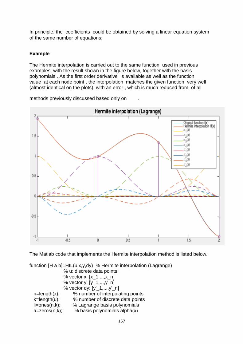
157

In principle, the coefficients could be obtained by solving a linear equation system

of the same number of equations:

Example

The Hermite interpolation is carried out to the same function used in previous examples, with the result shown in the figure below, together with the basis polynomials . As the first order derivative is available as well as the function value at each node point , the interpolation matches the given function very well (almost identical on the plots), with an error , which is much reduced from of all

methods previously discussed based only on .

The Matlab code that implements the Hermite interpolation method is listed below.

function [H a b]=HIL(u,x,y,dy) % Hermite interpolation (Lagrange) % u: discrete data points; % vector x: [x_1,...,x_n] % vector y: [y_1,...,y_n] % vector dy: [y'_1,...,y'_n] n=length(x); % number of interpolating points k=length(u); % number of discrete data points li=ones(n,k); % Lagrange basis polynomials a=zeros(n,k); % basis polynomials alpha(x)

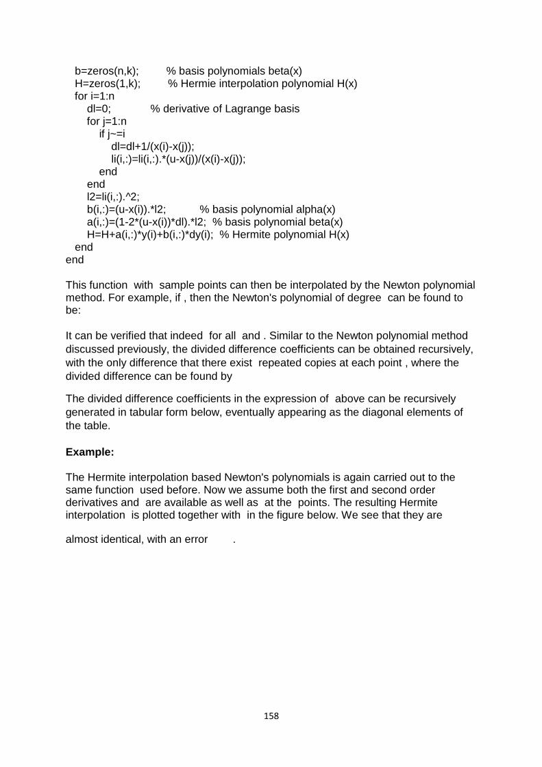
158

b=zeros(n,k); % basis polynomials beta(x) H=zeros(1,k); % Hermie interpolation polynomial H(x) for i=1:n dl=0; % derivative of Lagrange basis for j=1:n if j~=i dl=dl+1/(x(i)-x(j)); li(i,:)=li(i,:).*(u-x(j))/(x(i)-x(j)); end end l2=li(i,:).^2; b(i,:)=(u-x(i)).*l2; % basis polynomial alpha(x) a(i,:)=(1-2*(u-x(i))*dl).*l2; % basis polynomial beta(x) H=H+a(i,:)*y(i)+b(i,:)*dy(i); % Hermite polynomial H(x) end end

This function with sample points can then be interpolated by the Newton polynomial method. For example, if , then the Newton's polynomial of degree can be found to be:

It can be verified that indeed for all and . Similar to the Newton polynomial method

discussed previously, the divided difference coefficients can be obtained recursively,

with the only difference that there exist repeated copies at each point , where the

divided difference can be found by

The divided difference coefficients in the expression of above can be recursively

generated in tabular form below, eventually appearing as the diagonal elements of

the table.

Example:

The Hermite interpolation based Newton's polynomials is again carried out to the same function used before. Now we assume both the first and second order derivatives and are available as well as at the points. The resulting Hermite interpolation is plotted together with in the figure below. We see that they are

almost identical, with an error .

159

The Matlab code that implements this algorithm is listed below.

function [v]=HIN(u,x,dy) % Hermite interpolation (Newton) % u: discrete data points; % vector x: [x_1,...,x_n] % matrix dy contains m derivatives at each of the n points [n m]=size(dy); k=length(u); % number of discrete data points v=zeros(1,k); % interpolation results dd=DividedDifference2(x,dy); % get the divided difference array w=ones(1,k); for i=1:n p=u-x(i); for j=1:m l=(i-1)*m+j; % index of the coefficient v=v+dd(l,l).*w; % which is on the diagnal of array dd w=w.*p; end end end function dd=DividedDifference2(x,dy) % generate array of divided differences [n m]=size(dy); % n data points, m derivatives (0 to m-1) dd=zeros(n*m); % matrix of divided differences

160

z=zeros(1,n*m); k=1; for i=1:n % n data points for j=1:m % m derivatives (0 to m-1) at each point k=(i-1)*m+j; % row index z(k)=x(i); dd(k,1)=dy(i,1); % 0th divided difference in first column fprintf('%6.3f\t%6.3f\t',z(k),dd(k,1)); for l=2:k % column index for the remaining columns %fprintf('(%f %f)\n',dd(k,l-1),dd(k-1,l-1)); if dd(k,l-1)==dd(k-1,l-1) % left and top-left neighbors are repeated dd(k,l)=dy(i,l)/factorial(l-1); fprintf('k=%d, l=%d\n',k,l); pause else dd(k,l)=(dd(k,l-1)-dd(k-1,l-1))/(z(k)-z(k-l+1)); end fprintf('%6.3f\t',dd(k,l)); end fprintf('\n'); end end end

The array of divided differences generated by the function DividedDifference2 is given below, the elements along the diagonal are the coefficients in the Hermite polynomials.

In some cases, in engineering or real world technical problems, we are not interested to find the exact solution of a problem. If we have a good enough approximation, we can consider that we‘ve found the solution of the problem.

For example, if we want to compute the trigonometric function f(x)=sin(x) with a hand held calculator, we have two options:

use the actual trigonometric function sin(x), if the calculator has the function embedded (available if it‘s a scientific calculator)

use a polynomial as an approximation of the sin(x) function and compute the result with any calculator, or even by hand

In general, any mathematical function f(x), with some constraints, can be approximated by a polynomial P(x):

P(x)=a0+a1⋅x+a2⋅x2+…+an⋅xn

Weierstrass approximation theorem

First, let‘s put down what the theorem sounds like. After, we‘ll try to explain it a bit.

Theorem: For a given function f(x), which is defined and continuous on the interval [a, b], there is always a polynomial P(x), also defined on the interval [a, b], with the property:

|f(x)−P(x)|<ε

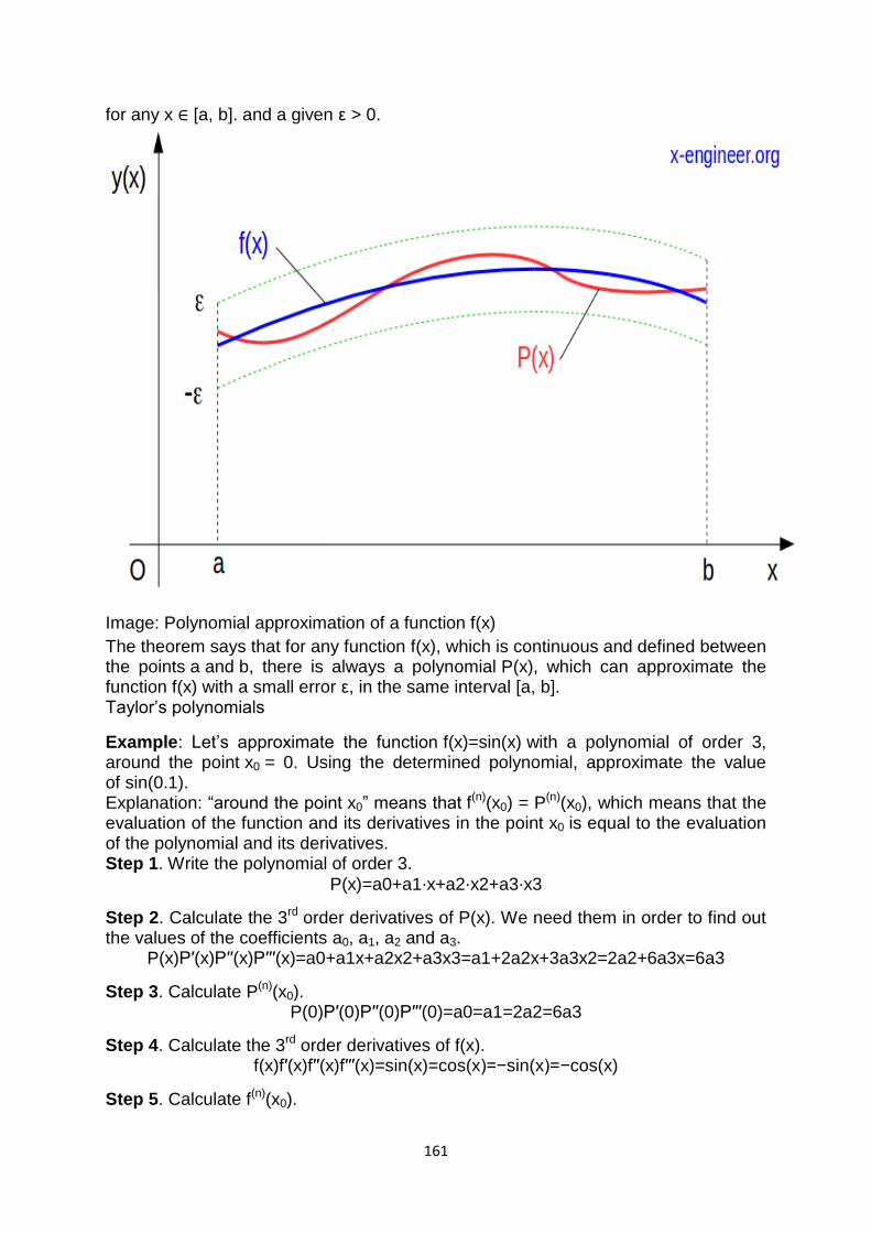
161

for any x ∈ [a, b]. and a given ε > 0.

Image: Polynomial approximation of a function f(x)

The theorem says that for any function f(x), which is continuous and defined between the points a and b, there is always a polynomial P(x), which can approximate the function f(x) with a small error ε, in the same interval [a, b]. Taylor‘s polynomials

Example: Let‘s approximate the function f(x)=sin(x) with a polynomial of order 3, around the point x0 = 0. Using the determined polynomial, approximate the value of sin(0.1). Explanation: ―around the point x0‖ means that f(n)(x0) = P(n)(x0), which means that the evaluation of the function and its derivatives in the point x0 is equal to the evaluation of the polynomial and its derivatives. Step 1. Write the polynomial of order 3.

P(x)=a0+a1⋅x+a2⋅x2+a3⋅x3

Step 2. Calculate the 3rd order derivatives of P(x). We need them in order to find out the values of the coefficients a0, a1, a2 and a3.

P(x)P′(x)P′′(x)P′′′(x)=a0+a1x+a2x2+a3x3=a1+2a2x+3a3x2=2a2+6a3x=6a3

Step 3. Calculate P(n)(x0). P(0)P′(0)P′′(0)P′′′(0)=a0=a1=2a2=6a3

Step 4. Calculate the 3rd order derivatives of f(x). f(x)f′(x)f′′(x)f′′′(x)=sin(x)=cos(x)=−sin(x)=−cos(x)

Step 5. Calculate f(n)(x0).

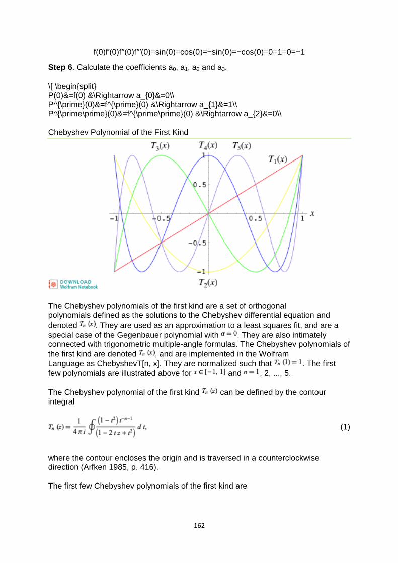
162

f(0)f′(0)f′′(0)f′′′(0)=sin(0)=cos(0)=−sin(0)=−cos(0)=0=1=0=−1

Step 6. Calculate the coefficients a0, a1, a2 and a3.

\[ \begin{split} P(0)&=f(0) &\Rightarrow a_{0}&=0\\ P^{\prime}(0)&=f^{\prime}(0) &\Rightarrow a_{1}&=1\\ P^{\prime\prime}(0)&=f^{\prime\prime}(0) &\Rightarrow a_{2}&=0\\

Chebyshev Polynomial of the First Kind

The Chebyshev polynomials of the first kind are a set of orthogonal polynomials defined as the solutions to the Chebyshev differential equation and

denoted . They are used as an approximation to a least squares fit, and are a

special case of the Gegenbauer polynomial with . They are also intimately connected with trigonometric multiple-angle formulas. The Chebyshev polynomials of

the first kind are denoted , and are implemented in the Wolfram

Language as ChebyshevT[n, x]. They are normalized such that . The first

few polynomials are illustrated above for and , 2, ..., 5.

The Chebyshev polynomial of the first kind can be defined by the contour integral

(1)

where the contour encloses the origin and is traversed in a counterclockwise direction (Arfken 1985, p. 416).

The first few Chebyshev polynomials of the first kind are

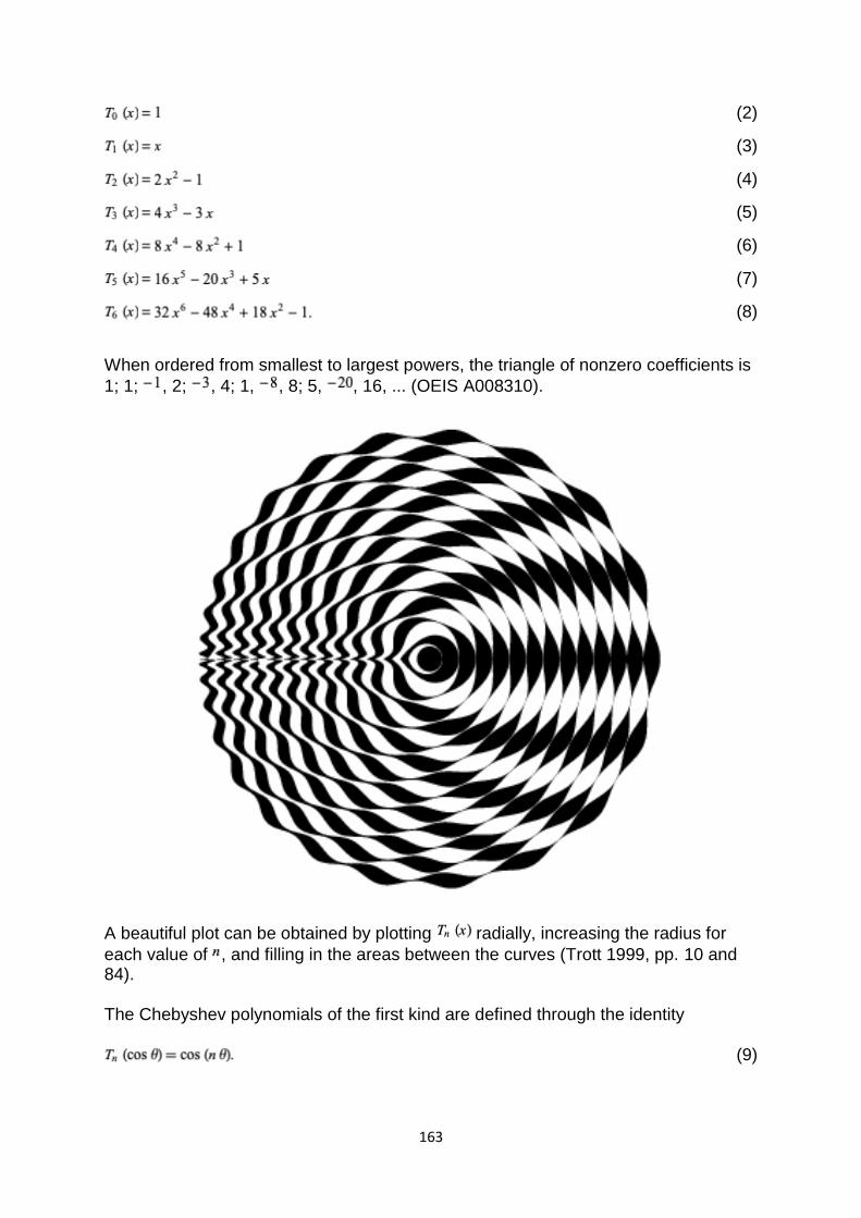
163

(2)

(3)

(4)

(5)

(6)

(7)

(8)

When ordered from smallest to largest powers, the triangle of nonzero coefficients is

1; 1; , 2; , 4; 1, , 8; 5, , 16, ... (OEIS A008310).

A beautiful plot can be obtained by plotting radially, increasing the radius for

each value of , and filling in the areas between the curves (Trott 1999, pp. 10 and 84).

The Chebyshev polynomials of the first kind are defined through the identity

(9)

164

The Chebyshev polynomials of the first kind can be obtained from the generating functions

(10)

(11)

and

(12)

(13)

for and (Beeler et al. 1972, Item 15). (A closely related generating function is the basis for the definition of Chebyshev polynomial of the second kind.)

A direct representation is given by

(14)

The polynomials can also be defined in terms of the sums

(15)

(16)

(17)

where is a binomial coefficient and is the floor function, or the product

(18)

(Zwillinger 1995, p. 696).

also satisfy the curious determinant equation

165

(19)

(Nash 1986).

The Chebyshev polynomials of the first kind are a special case of the Jacobi

polynomials with ,

(20)

(21)

where is a hypergeometric function (Koekoek and Swarttouw 1998).

Zeros occur when

(22)

for , 2, ..., . Extrema occur for

(23)

where . At maximum, , and at minimum, .

The Chebyshev polynomials are orthogonal polynomials with respect to

the weighting function

(24)

where is the Kronecker delta. Chebyshev polynomials of the first kind satisfy the additional discrete identity

166

(25)

where for , ..., are the zeros of .

They also satisfy the recurrence relations

(26)

(27)

for , as well as

(28)

(29)

(Watkins and Zeitlin 1993; Rivlin 1990, p. 5).

They have a complex integral representation

(30)

and a Rodrigues representation

(31)

Using a fast Fibonacci transform with multiplication law

(32)

gives

(33)

Using Gram-Schmidt orthonormalization in the range ( ,1) with weighting

function gives

(34)

167

(35)

(36)

(37)

(38)

(39)

(40)

etc. Normalizing such that gives the Chebyshev polynomials of the first kind.

The Chebyshev polynomial of the first kind is related to the Bessel function of the

first kind and modified Bessel function of the first kind by the relations

(41)

(42)

Letting allows the Chebyshev polynomials of the first kind to be written as

(43)

(44)

The second linearly dependent solution to the transformed differential equation

(45)

is then given by

(46)

(47)

which can also be written

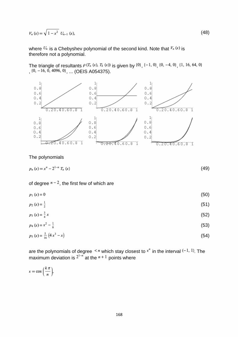
168

(48)

where is a Chebyshev polynomial of the second kind. Note that is therefore not a polynomial.

The triangle of resultants is given by , , ,

, , ... (OEIS A054375).

The polynomials

(49)

of degree , the first few of which are

(50)

(51)

(52)

(53)

(54)

are the polynomials of degree which stay closest to in the interval . The

maximum deviation is at the points where

169

UNIT -V

Numerical Differentiation and Integration:

Introduction

Differentiation and integration are basic mathematical operations with a wide range

of applications in many areas of science. It is therefore important to have good

methods to compute and manipulate derivatives and integrals. You probably learnt

the basic rules of differentiation and integration in school — symbolic methods

suitable for pencil-and-paper calculations. These are important, and most derivatives

can be computed this way. Integration however, is different, and most integrals

cannot be determined with symbolic methods like the ones you learnt in school.

Another complication is the fact that in practical applications a function is only known

at a few points. For example, we may measure the position of a car every minute via

a GPS (Global Positioning System) unit, and we want to compute its speed. If the

position is known as a continuous function of time, we can find the speed by

differentiating this function. But when the position is only known at isolated times,

this is not possible. The same applies to integrals. The solution, both when it comes

to integrals that cannot be determined by the usual methods, and functions that are

only known at isolated points, is to use approximate methods of differentiation and

integration. In our context, these are going to be numerical methods. We are going to

present a number of methods for doing numerical integration and differentiation, but

more importantly, we are going to present a general strategy for deriving such

methods. In this way you will not only have a number of methods available to you,

but you will also be able to develop new methods, tailored to special situations that

you may encounter. We use the same general strategy for deriving both numerical

integration and numerical differentiation methods. The basic idea is to evaluate a

function at a few points, find the polynomial that interpolates the function at these

points, and use the derivative or integral of the polynomial as an approximation to

the function. This technique also allows us to keep track of the so-called truncation

error, the mathematical error committed by integrating or differentiating the

polynomial instead of the function itself. However, when it comes to roundoff error,

we have to treat differentiation and integration differently: Numerical integration is

very insensitive to round-off errors, while numerical differentiation behaves in the

opposite way; it is very sensitive to round-off errors. 11.1 A simple method for

numerical differentiation We start by studying numerical differentiation. We first

introduce the simplest method, derive its error, and its sensitivity to round-off errors.

The procedure used here for deriving the method and analysing the error is used

over again in later sections to derive and analyse additional methods. Let us first

make it clear what numerical differentiation is. Problem 11.1 (Numerical

differentiation). Let f be a given function that is only known at a number of isolated

points. The problem of numerical differentiation is to compute an approximation to

the derivative f 0 of f by suitable combinations of the known values of f . A typical

170

example is that f is given by a computer program (more specifically a function,

procedure or method, depending on you choice of programming language), and you

can call the program with a floating-point argument x and receive back a floating-

point approximation of f (x). The challenge is to compute an approximation to f 0 (a)

for some real number a when the only aid we have at our disposal is the program to

compute values of f . 11.1.1 The basic idea Since we are going to compute

derivatives, we must be clear about they are defined. Recall that f 0 (a) is defined by

f 0 (a) = lim h→0 f (a +h)− f (a) h . (11.1) In the following we will assume that this limit

exists; i.e., that f is differentiable. From (11.1) we immediately have a natural

approximation to f 0 (a); we simply 228 pick a positive h and use the approximation f

0 (a) ≈ f (a +h)− f (a) h . (11.2) Note that this corresponds to approximating f by the

straight line p1 that interpolates f at a and a −h, and then using p 0 1 (a) as an

approximation to f 0 (a). Observation 11.2. The derivative of f at a can be

approximated by f 0 (a) ≈ f (a +h)− f (a) h . In a practical situation, the number a

would be given, and we would have to locate the two nearest values a1 and a2 to

the left and right of a such that f (a1) and f (a2) can be found. Then we would use the

approximation f 0 (a) ≈ f (a2)− f (a1) a2 − a1 . In later sections, we will derive several

formulas like (11.2). Which formula to use for a specific example, and exactly how to

use it, will have to be decided in each case. Example 11.3. Let us test the

approximation (11.2) for the function f (x) = sinx at a = 0.5 (using 64-bit floating-point

numbers). In this case we have f 0 (x) = cosx so f 0 (a) = 0.87758256. This makes it

is easy to check the accuracy. We try with a few values of h and find h ¡ f (a +h)− f

(a) ¢±h E1(f ;a,h) 10−1 0.8521693479 2.5×10−2 10−2 0.8751708279 2.4×10−3 10−3

0.8773427029 2.4×10−4 10−4 0.8775585892 2.4×10−5 10−5 0.8775801647

2.4×10−6 10−6 0.8775823222 2.4×10−7 where E1(f ;a,h) = f (a)− ¡ f (a+h)− f (a) ¢±h.

In other words, the approximation seems to improve with decreasing h, as expected.

More precisely, when h is reduced by a factor of 10, the error is reduced by the same

factor.

Numerical Differentiation

Numerical differentiation is the process of finding the numerical value of a derivative of a given function at a given point. In general, numerical differentiation is more difficult than numerical integration. This is because while numerical integration requires only good continuity properties of the function being integrated, numerical differentiation requires more complicated properties such as Lipschitz classes. Numerical differentiation is implemented as ND[f, x, x0, Scale -> scale] in the Wolfram Language package NumericalCalculus` .

There are many applications where derivatives need to be computed numerically. The simplest approach simply uses the definition of the derivative

for some small numerical value of .

171

A Numerical Integration

Numerical integration of the equations described in this chapter is required to generate simulations of material response to a given loading history. It is important to consider the techniques of numerical integration for reasons of computational economy and compatibility with structural mechanics codes in which the constitutive equations may be employed. The MATMOD-4V-DISTORTION equations are numerically integrated using the Gear Method for stiff differential equations. Such methods are necessary because of the inherent mathematical stiffness of any unified model, including MATMOD. The stiffness of these equations arises from the coupling of nonelastic and elastic strains to calculate the total strain, and the fact that ɛ˙ is a strong function of σ. Analogous problems arise in integrating the structure evolution equations, adding to the difficulty of the integration. To attack these problems and to provide a better interface with existing finite-element structural mechanics codes, the NONSS (NONlinear System Solver) method was developed (Tanaka, 1983; Tanaka and Miller, 1988; Miller and Tanaka, 1988) and employed for integration of the three-dimensional MATMOD-BSSOL equations (Henshall, 1987). Details of the methods used to integrate the MATMOD-4V-DISTORTION and MATMOD-BSSOL equations are provided elsewhere (Helling, 1986; Henshall, 1987; Miller, 1987; Tanaka, 1983; Tanaka and Miller, 1988). The Fortran programs embodying these numerical integration schemes are available for both models through any of the authors. Recently, the NONSS method was incorporated into a finite-element code by Chellapandi and Alwar (1996). They used the 23-parameter Chaboche viscoplastic constitutive model and compared the computational efficiency of NONSS against their standard Self-Adaptive Forward Euler (SAFE) method. For their three most complicated cases including cyclic loading and behavior around notches, the ratios of computational time by SAFE to that using NONSS were 8.47, 9.7, and 7.33, respectively. This indicates that considerable time can be saved in finite-element analyses involving advanced unified constitutive equations by employing numerical methods. Numerical integration procedures have been applied frequently in order to avoid some of the assumptions inherent in the above approximate treatments. Among the most straightforward of these is the method utilized in Nordheim's33 code ZUT, which calculates effective resonance integrals for isolated resonances in a two region lattice geometry. As discussed in connection with equation (22) in Section 3.1 the shielding function in the fuel f0(u) for an isolated resonance may be obtained by solving the integral equation for the collision density per unit energy ψ0(u) expressed as a function of lethargy. The loss of neutrons due to absorption is then accounted for by an exponential dependence of the slowing down density on the group resonance integral for absorption, equation (12). The function ψ0(u) is obtained by solving the first of the two integral equations shown in equation (36), to which the reciprocity relation, equation (41), is applied, giving (97)ψ0(u)=P0(u)∑iTiψ0+{1−P0(u)}×{Σt(u)}0(ΣB)1∑jTjψ1.

172

The resonance integrals are then obtained from equation (26) as applied to the fuel, (98)(Ieffx)i=∫resσix(u){Σt(u)}0Eψ0(u)du.

The ZUT code simplifies equation (97) by assuming that for slowing down by the moderator nuclides the NR approximation holds. As discussed in connection with equation (27), the equation then reduces to (99)ψ0(u)=P0(u)∑iTiψ0+{1−P0(u)}{Σt(u)}0/E

which is an integral equation for ψ0(u), the integral operators Ti being defined in equation (25). The ZUT program solves equation (99) by Simpson integrations over a fine lethargy mesh, which covers the central portion of each individual resonance, this lethargy range being defined to be five practical widths √(σto/σtp)Γ/E0,, or ten Doppler widths 2Δ/E0, whichever is the larger. The small wing corrections outside this range are added as unshielded unbroadened resonance integrals in a 1/E flux. The Simpson integration of equation (99), and subsequent trapezium integration of equation (98), start at the low lethargy limit of the central portion of the resonance, and proceed on a fine lethargy mesh, selected so that an integral number of mesh intervals cover the range of integration in equation (98). The masses of the nuclides i are adjusted slightly, as required, in order that an even number of mesh intervals cover the integration range in Tiψ0 of equation (99). Outside the central portion of the resonance ψ0(u) is assumed to have the asymptotic value (ΣB)0/E or (ΣB)0 e

u/E0. Consequently, the solution of equation (99) can proceed successively from mesh point to mesh point by Simpson integration, the value ψ0(u) at the next mesh point being the only unknown. The successive contributions to the integral in equation (98) are calculated as soon as the ψ0(u) becomes known at each new mesh point (see also Section 4.3).

One-dimensional integration

J.E. Akin, in Finite Element Analysis with Error Estimators, 2005 4.4 Numerical integration

Numerical integration is simply a procedure that approximates (usually) an integral by a summation. To review this subject we refer to Fig. 4.2. Recall that the integral

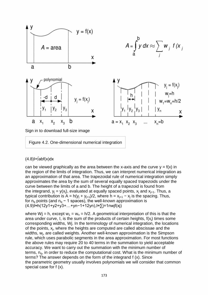
173

Sign in to download full-size image

Figure 4.2. One-dimensional numerical integration

(4.8)I=∫abf(x)dx

can be viewed graphically as the area between the x-axis and the curve y = f(x) in the region of the limits of integration. Thus, we can interpret numerical integration as an approximation of that area. The trapezoidal rule of numerical integration simply approximates the area by the sum of several equally spaced trapezoids under the curve between the limits of a and b. The height of a trapezoid is found from the integrand, yj = y(xj), evaluated at equally spaced points, xj and xj+1. Thus, a typical contribution is A = h(yj + yj+1)/2, where h = xj+1 − xj is the spacing. Thus, for nq points (and nq − 1 spaces), the well-known approximation is (4.9)I≈h(12y1+y2+y3+…+yn−1+12yn),I≈∑j=1nwjf(xj)

where Wj = h, except w1 = wn = h/2. A geometrical interpretation of this is that the area under curve, I, is the sum of the products of certain heights, f(xj) times some corresponding widths, Wj. In the terminology of numerical integration, the locations of the points, xj, where the heights are computed are called abscissae and the widths, wj, are called weights. Another well-known approximation is the Simpson rule, which uses parabolic segments in the area approximation. For most functions the above rules may require 20 to 40 terms in the summation to yield acceptable accuracy. We want to carry out the summation with the minimum number of terms, nq, in order to reduce the computational cost. What is the minimum number of terms? The answer depends on the form of the integrand f (x). Since the parametric geometry usually involves polynomials we will consider that common special case for f (x).

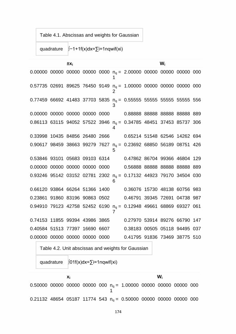
174

Table 4.1. Abscissas and weights for Gaussian

quadrature ∫−1+1f(x)dx=∑i=1nqwif(xi)

±xi

Wi

0.00000 00000 00000 00000 0000 nq = 1

2.00000 00000 00000 00000 000

0.57735 02691 89625 76450 9149 nq = 2

1.00000 00000 00000 00000 000

0.77459 66692 41483 37703 5835 nq = 3

0.55555 55555 55555 55555 556

0.00000 00000 00000 00000 0000 0.88888 88888 88888 88888 889

0.86113 63115 94052 57522 3946 nq = 4

0.34785 48451 37453 85737 306

0.33998 10435 84856 26480 2666 0.65214 51548 62546 14262 694

0.90617 98459 38663 99279 7627 nq = 5

0.23692 68850 56189 08751 426

0.53846 93101 05683 09103 6314 0.47862 86704 99366 46804 129

0.00000 00000 00000 00000 0000 0.56888 88888 88888 88888 889

0.93246 95142 03152 02781 2302 nq = 6

0.17132 44923 79170 34504 030

0.66120 93864 66264 51366 1400 0.36076 15730 48138 60756 983

0.23861 91860 83196 90863 0502 0.46791 39345 72691 04738 987

0.94910 79123 42758 52452 6190 nq = 7

0.12948 49661 68869 69327 061

0.74153 11855 99394 43986 3865 0.27970 53914 89276 66790 147

0.40584 51513 77397 16690 6607 0.38183 00505 05118 94495 037

0.00000 00000 00000 00000 0000 0.41795 91836 73469 38775 510

Table 4.2. Unit abscissas and weights for Gaussian

quadrature ∫01f(x)dx=∑i=1nqwif(xi)

xi

Wi

0.50000 00000 00000 00000 000 nq = 1

1.00000 00000 00000 00000 000

0.21132 48654 05187 11774 543 nq = 0.50000 00000 00000 00000 000

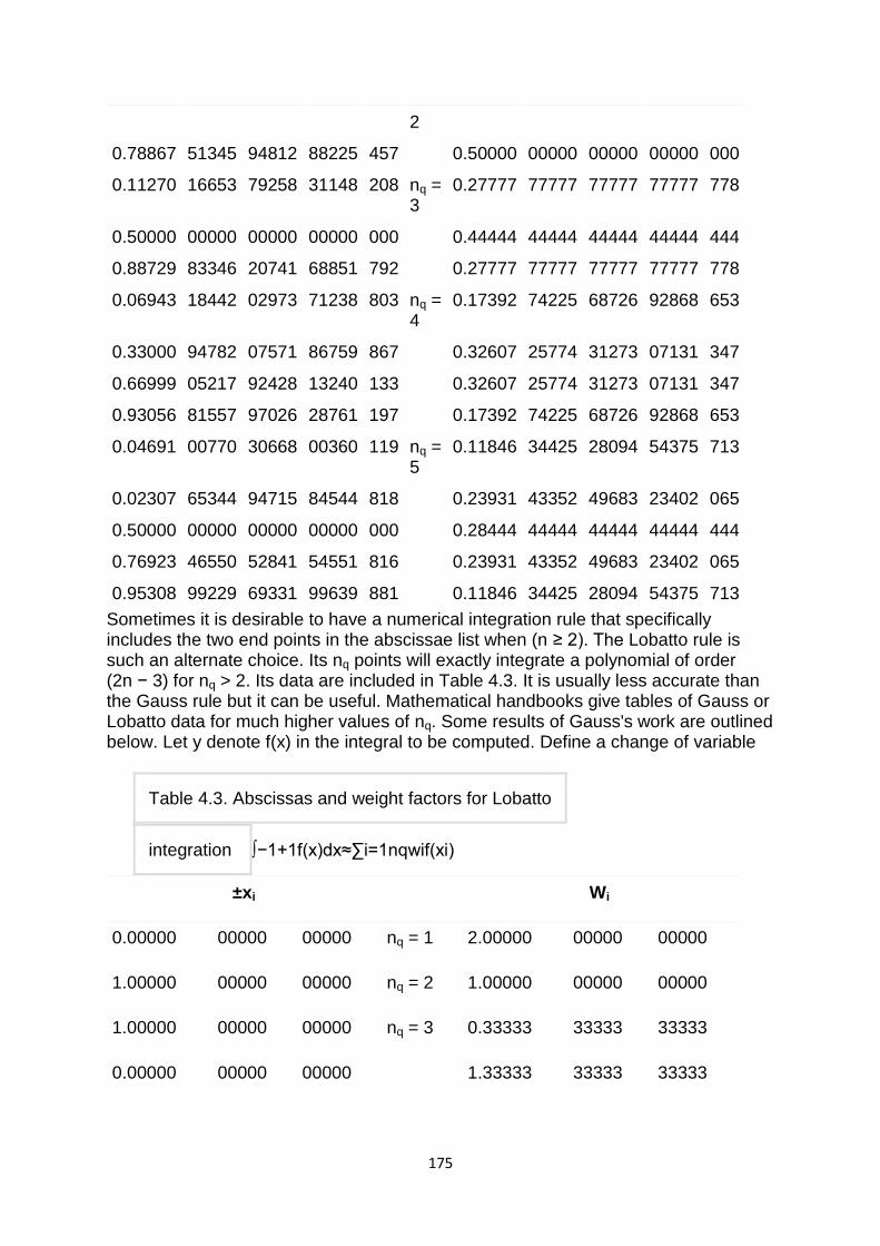
175

2

0.78867 51345 94812 88225 457 0.50000 00000 00000 00000 000

0.11270 16653 79258 31148 208 nq = 3

0.27777 77777 77777 77777 778

0.50000 00000 00000 00000 000 0.44444 44444 44444 44444 444

0.88729 83346 20741 68851 792 0.27777 77777 77777 77777 778

0.06943 18442 02973 71238 803 nq = 4

0.17392 74225 68726 92868 653

0.33000 94782 07571 86759 867 0.32607 25774 31273 07131 347

0.66999 05217 92428 13240 133 0.32607 25774 31273 07131 347

0.93056 81557 97026 28761 197 0.17392 74225 68726 92868 653

0.04691 00770 30668 00360 119 nq = 5

0.11846 34425 28094 54375 713

0.02307 65344 94715 84544 818 0.23931 43352 49683 23402 065

0.50000 00000 00000 00000 000 0.28444 44444 44444 44444 444

0.76923 46550 52841 54551 816 0.23931 43352 49683 23402 065

0.95308 99229 69331 99639 881 0.11846 34425 28094 54375 713

Sometimes it is desirable to have a numerical integration rule that specifically includes the two end points in the abscissae list when (n ≥ 2). The Lobatto rule is such an alternate choice. Its nq points will exactly integrate a polynomial of order (2n − 3) for nq > 2. Its data are included in Table 4.3. It is usually less accurate than the Gauss rule but it can be useful. Mathematical handbooks give tables of Gauss or Lobatto data for much higher values of nq. Some results of Gauss's work are outlined below. Let y denote f(x) in the integral to be computed. Define a change of variable

Table 4.3. Abscissas and weight factors for Lobatto

integration ∫−1+1f(x)dx≈∑i=1nqwif(xi)

±xi

Wi

0.00000 00000 00000 nq = 1 2.00000 00000 00000

1.00000 00000 00000 nq = 2 1.00000 00000 00000

1.00000 00000 00000 nq = 3 0.33333 33333 33333

0.00000 00000 00000 1.33333 33333 33333

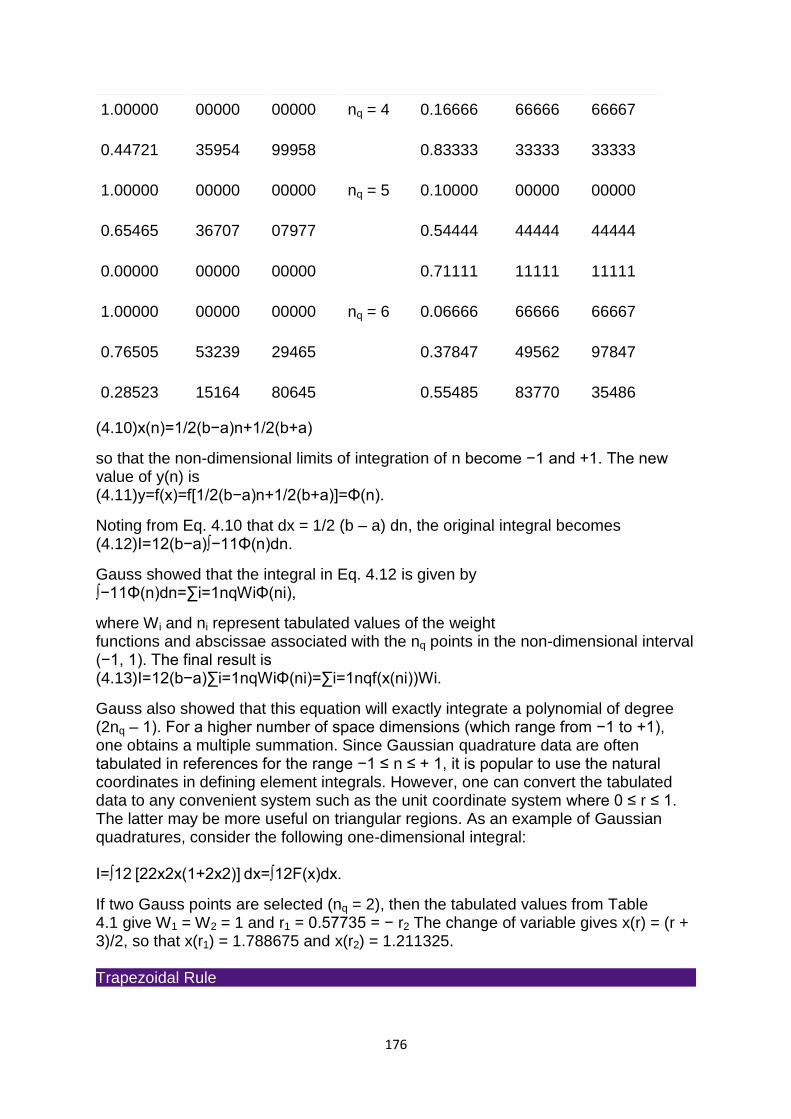
176

1.00000 00000 00000 nq = 4 0.16666 66666 66667

0.44721 35954 99958 0.83333 33333 33333

1.00000 00000 00000 nq = 5 0.10000 00000 00000

0.65465 36707 07977 0.54444 44444 44444

0.00000 00000 00000 0.71111 11111 11111

1.00000 00000 00000 nq = 6 0.06666 66666 66667

0.76505 53239 29465 0.37847 49562 97847

0.28523 15164 80645 0.55485 83770 35486

(4.10)x(n)=1/2(b−a)n+1/2(b+a)

so that the non-dimensional limits of integration of n become −1 and +1. The new value of y(n) is (4.11)y=f(x)=f[1/2(b−a)n+1/2(b+a)]=Φ(n).

Noting from Eq. 4.10 that dx = 1/2 (b – a) dn, the original integral becomes (4.12)I=12(b−a)∫−11Φ(n)dn.

Gauss showed that the integral in Eq. 4.12 is given by ∫−11Φ(n)dn=∑i=1nqWiΦ(ni),

where Wi and ni represent tabulated values of the weight functions and abscissae associated with the nq points in the non-dimensional interval (−1, 1). The final result is (4.13)I=12(b−a)∑i=1nqWiΦ(ni)=∑i=1nqf(x(ni))Wi.

Gauss also showed that this equation will exactly integrate a polynomial of degree (2nq – 1). For a higher number of space dimensions (which range from −1 to +1), one obtains a multiple summation. Since Gaussian quadrature data are often tabulated in references for the range −1 ≤ n ≤ + 1, it is popular to use the natural coordinates in defining element integrals. However, one can convert the tabulated data to any convenient system such as the unit coordinate system where 0 ≤ r ≤ 1. The latter may be more useful on triangular regions. As an example of Gaussian quadratures, consider the following one-dimensional integral: I=∫12 [22x2x(1+2x2)] dx=∫12F(x)dx.

If two Gauss points are selected (nq = 2), then the tabulated values from Table 4.1 give W1 = W2 = 1 and r1 = 0.57735 = − r2 The change of variable gives x(r) = (r + 3)/2, so that x(r1) = 1.788675 and x(r2) = 1.211325. Trapezoidal Rule

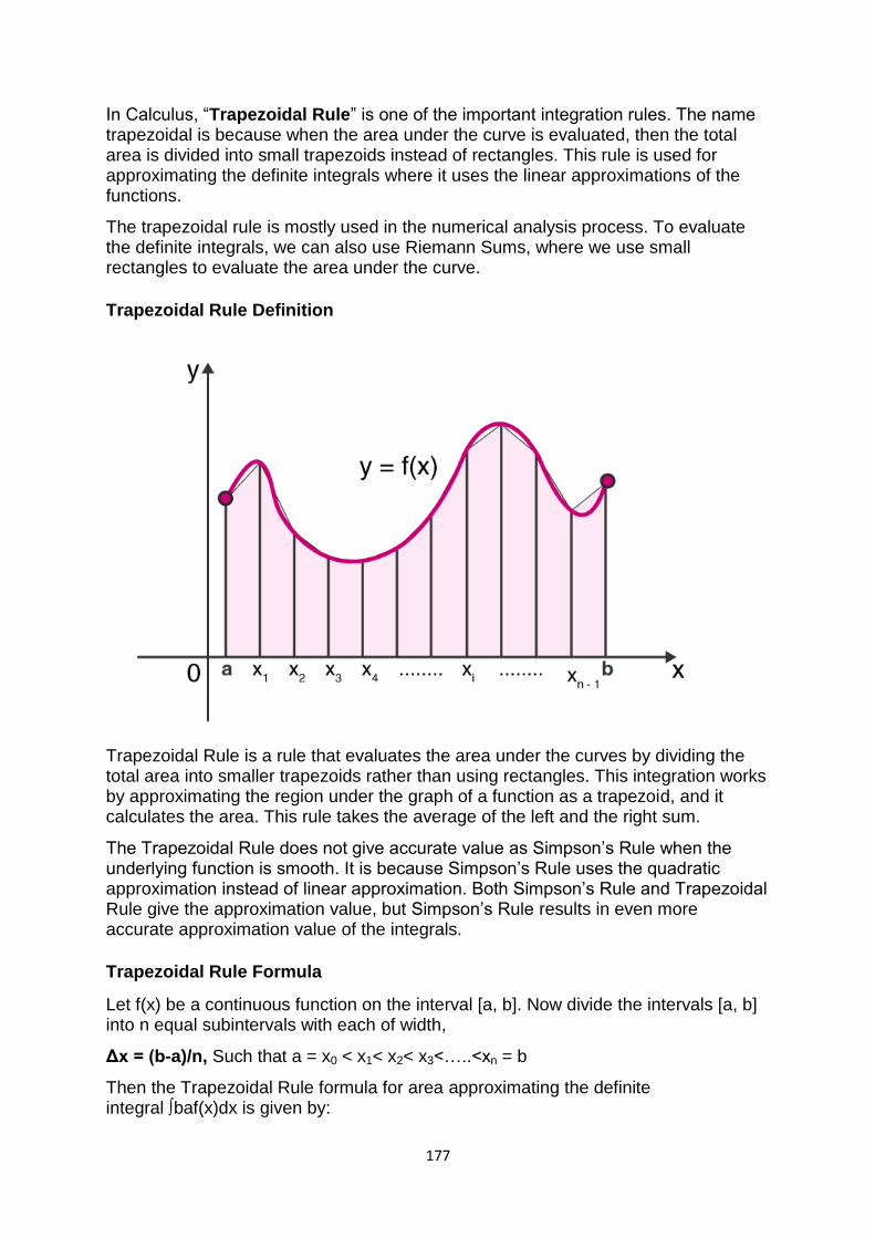
177

In Calculus, ―Trapezoidal Rule‖ is one of the important integration rules. The name trapezoidal is because when the area under the curve is evaluated, then the total area is divided into small trapezoids instead of rectangles. This rule is used for approximating the definite integrals where it uses the linear approximations of the functions.

The trapezoidal rule is mostly used in the numerical analysis process. To evaluate the definite integrals, we can also use Riemann Sums, where we use small rectangles to evaluate the area under the curve.

Trapezoidal Rule Definition

Trapezoidal Rule is a rule that evaluates the area under the curves by dividing the total area into smaller trapezoids rather than using rectangles. This integration works by approximating the region under the graph of a function as a trapezoid, and it calculates the area. This rule takes the average of the left and the right sum.

The Trapezoidal Rule does not give accurate value as Simpson‘s Rule when the underlying function is smooth. It is because Simpson‘s Rule uses the quadratic approximation instead of linear approximation. Both Simpson‘s Rule and Trapezoidal Rule give the approximation value, but Simpson‘s Rule results in even more accurate approximation value of the integrals.

Trapezoidal Rule Formula

Let f(x) be a continuous function on the interval [a, b]. Now divide the intervals [a, b] into n equal subintervals with each of width,

Δx = (b-a)/n, Such that a = x0 < x1< x2< x3<…..<xn = b

Then the Trapezoidal Rule formula for area approximating the definite integral ∫baf(x)dx is given by:

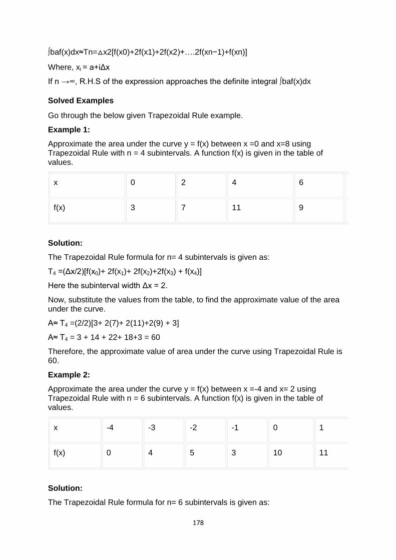
178

∫baf(x)dx≈Tn=△x2[f(x0)+2f(x1)+2f(x2)+….2f(xn−1)+f(xn)]

Where, xi = a+iΔx

If n →∞, R.H.S of the expression approaches the definite integral ∫baf(x)dx

Solved Examples

Go through the below given Trapezoidal Rule example.

Example 1:

Approximate the area under the curve y = f(x) between x =0 and x=8 using Trapezoidal Rule with n = 4 subintervals. A function f(x) is given in the table of values.

x 0 2 4 6 8

f(x) 3 7 11 9 3

Solution:

The Trapezoidal Rule formula for n= 4 subintervals is given as:

T4 =(Δx/2)[f(x0)+ 2f(x1)+ 2f(x2)+2f(x3) + f(x4)]

Here the subinterval width Δx = 2.

Now, substitute the values from the table, to find the approximate value of the area under the curve.

A≈ T4 =(2/2)[3+ 2(7)+ 2(11)+2(9) + 3]

A≈ T4 = 3 + 14 + 22+ 18+3 = 60

Therefore, the approximate value of area under the curve using Trapezoidal Rule is 60.

Example 2:

Approximate the area under the curve y = f(x) between x =-4 and x= 2 using Trapezoidal Rule with n = 6 subintervals. A function f(x) is given in the table of values.

x -4 -3 -2 -1 0 1 2

f(x) 0 4 5 3 10 11 2

Solution:

The Trapezoidal Rule formula for n= 6 subintervals is given as:

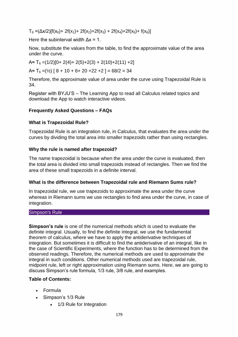
179

T6 =(Δx/2)[f(x0)+ 2f(x1)+ 2f(x2)+2f(x3) + 2f(x4)+2f(x5)+ f(x6)]

Here the subinterval width Δx = 1.

Now, substitute the values from the table, to find the approximate value of the area under the curve.

A≈ T6 =(1/2)[0+ 2(4)+ 2(5)+2(3) + 2(10)+2(11) +2]

A≈ T6 =(½) [ 8 + 10 + 6+ 20 +22 +2 ] = 68/2 = 34

Therefore, the approximate value of area under the curve using Trapezoidal Rule is 34.

Register with BYJU‘S – The Learning App to read all Calculus related topics and download the App to watch interactive videos.

Frequently Asked Questions – FAQs

What is Trapezoidal Rule?

Trapezoidal Rule is an integration rule, in Calculus, that evaluates the area under the

curves by dividing the total area into smaller trapezoids rather than using rectangles.

Why the rule is named after trapezoid?

The name trapezoidal is because when the area under the curve is evaluated, then

the total area is divided into small trapezoids instead of rectangles. Then we find the

area of these small trapezoids in a definite interval.

What is the difference between Trapezoidal rule and Riemann Sums rule?

In trapezoidal rule, we use trapezoids to approximate the area under the curve

whereas in Riemann sums we use rectangles to find area under the curve, in case of

integration.

Simpson's Rule

Simpson’s rule is one of the numerical methods which is used to evaluate the definite integral. Usually, to find the definite integral, we use the fundamental theorem of calculus, where we have to apply the antiderivative techniques of integration. But sometimes it is difficult to find the antiderivative of an integral, like in the case of Scientific Experiments, where the function has to be determined from the observed readings. Therefore, the numerical methods are used to approximate the integral in such conditions. Other numerical methods used are trapezoidal rule, midpoint rule, left or right approximation using Riemann sums. Here, we are going to discuss Simpson‘s rule formula, 1/3 rule, 3/8 rule, and examples.

Table of Contents:

Formula

Simpson‘s 1/3 Rule

1/3 Rule for Integration

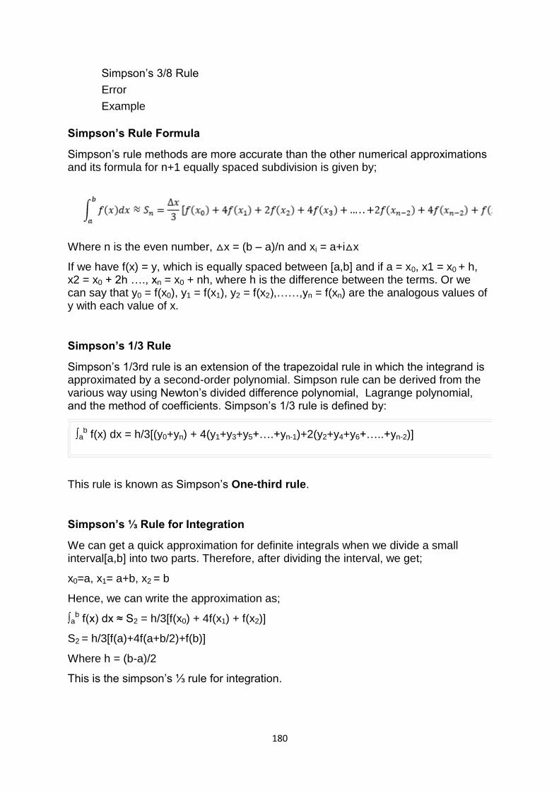
180

Simpson‘s 3/8 Rule

Error

Example

Simpson’s Rule Formula

Simpson‘s rule methods are more accurate than the other numerical approximations and its formula for n+1 equally spaced subdivision is given by;

Where n is the even number, △x = (b – a)/n and xi = a+i△x

If we have f(x) = y, which is equally spaced between [a,b] and if a = x0, x1 = x0 + h, x2 = x0 + 2h …., xn = x0 + nh, where h is the difference between the terms. Or we can say that y0 = f(x0), y1 = f(x1), y2 = f(x2),……,yn = f(xn) are the analogous values of y with each value of x.

Simpson’s 1/3 Rule

Simpson‘s 1/3rd rule is an extension of the trapezoidal rule in which the integrand is approximated by a second-order polynomial. Simpson rule can be derived from the various way using Newton‘s divided difference polynomial, Lagrange polynomial, and the method of coefficients. Simpson‘s 1/3 rule is defined by:

∫ab f(x) dx = h/3[(y0+yn) + 4(y1+y3+y5+….+yn-1)+2(y2+y4+y6+…..+yn-2)]

This rule is known as Simpson‘s One-third rule.

Simpson’s ⅓ Rule for Integration

We can get a quick approximation for definite integrals when we divide a small interval[a,b] into two parts. Therefore, after dividing the interval, we get;

x0=a, x1= a+b, x2 = b

Hence, we can write the approximation as;

∫ab f(x) dx ≈ S2 = h/3[f(x0) + 4f(x1) + f(x2)]

S2 = h/3[f(a)+4f(a+b/2)+f(b)]

Where h = (b-a)/2

This is the simpson‘s ⅓ rule for integration.

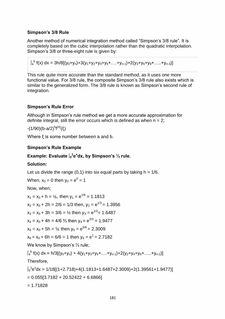
181

Simpson’s 3/8 Rule

Another method of numerical integration method called ―Simpson‘s 3/8 rule‖. It is completely based on the cubic interpolation rather than the quadratic interpolation. Simpson‘s 3/8 or three-eight rule is given by:

∫ab f(x) dx = 3h/8[(y0+yn)+3(y1+y2+y4+y5+….+yn-1)+2(y3+y6+y9+…..+yn-3)]

This rule quite more accurate than the standard method, as it uses one more functional value. For 3/8 rule, the composite Simpson‘s 3/8 rule also exists which is similar to the generalized form. The 3/8 rule is known as Simpson‘s second rule of integration.

Simpson’s Rule Error

Although in Simpson‘s rule method we get a more accurate approximation for definite integral, still the error occurs which is defined as when n = 2;

-(1/90)(b-a/2)5f(4)(ξ)

Where ξ is some number between a and b.

Simpson’s Rule Example

Example: Evaluate ∫01exdx, by Simpson’s ⅓ rule.

Solution:

Let us divide the range (0,1) into six equal parts by taking h = 1/6.

When, x0 = 0 then y0 = e0 = 1

Now, when;

x1 = x0 + h = ⅙, then y1 = e1/6 = 1.1813

x2 = x0 + 2h = 2/6 = 1/3 then, y2 = e1/3 = 1.3956

x3 = x0 + 3h = 3/6 = ½ then y3 = e1/2= 1.6487

x4 = x0 + 4h = 4/6 ⅔ then y4 = e2/3 = 1.9477

x5 = x0 + 5h = ⅚ then y5 = e5/6 = 2.3009

x6 = x0 + 6h = 6/6 = 1 then y6 = e1 = 2.7182

We know by Simpson‘s ⅓ rule;

∫ab f(x) dx = h/3[(y0+yn) + 4(y1+y3+y5+….+yn-1)+2(y2+y4+y6+…..+yn-2)]

Therefore,

∫01exdx = 1/18[(1+2.718)+4(1.1813+1.6487+2.3009)+2(1.39561+1.9477)]

= 0.055[3.7182 + 20.52422 + 6.6866]

= 1.71828

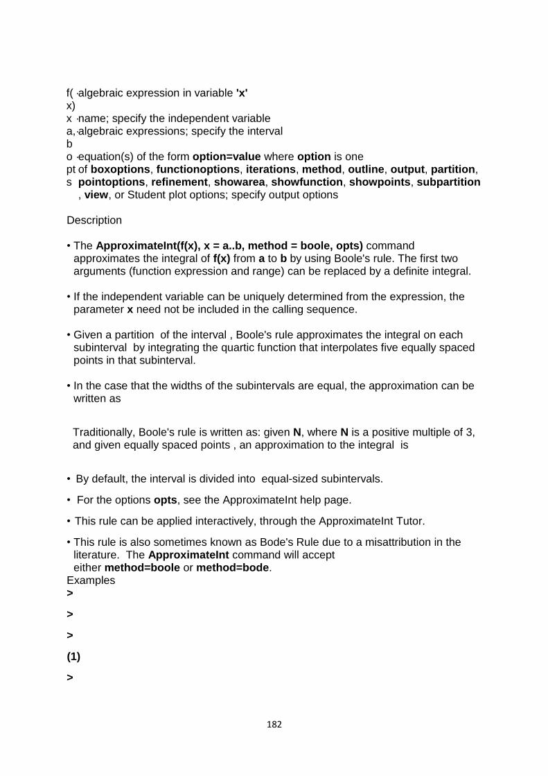
182

f(x)

- algebraic expression in variable 'x'

x - name; specify the independent variable a, b

- algebraic expressions; specify the interval

opts

- equation(s) of the form option=value where option is one of boxoptions, functionoptions, iterations, method, outline, output, partition, pointoptions, refinement, showarea, showfunction, showpoints, subpartition, view, or Student plot options; specify output options

Description

• The ApproximateInt(f(x), x = a..b, method = boole, opts) command approximates the integral of f(x) from a to b by using Boole's rule. The first two arguments (function expression and range) can be replaced by a definite integral.

• If the independent variable can be uniquely determined from the expression, the parameter x need not be included in the calling sequence.

• Given a partition of the interval , Boole's rule approximates the integral on each subinterval by integrating the quartic function that interpolates five equally spaced points in that subinterval.

• In the case that the widths of the subintervals are equal, the approximation can be written as

Traditionally, Boole's rule is written as: given N, where N is a positive multiple of 3, and given equally spaced points , an approximation to the integral is

• By default, the interval is divided into equal-sized subintervals.

• For the options opts, see the ApproximateInt help page.

• This rule can be applied interactively, through the ApproximateInt Tutor.

• This rule is also sometimes known as Bode's Rule due to a misattribution in the literature. The ApproximateInt command will accept either method=boole or method=bode.

Examples

>

>

>

(1)

>

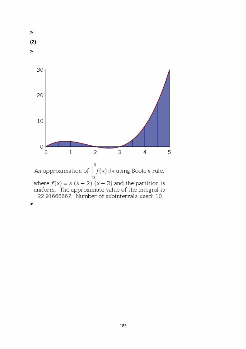
183

>

(2)

>

>

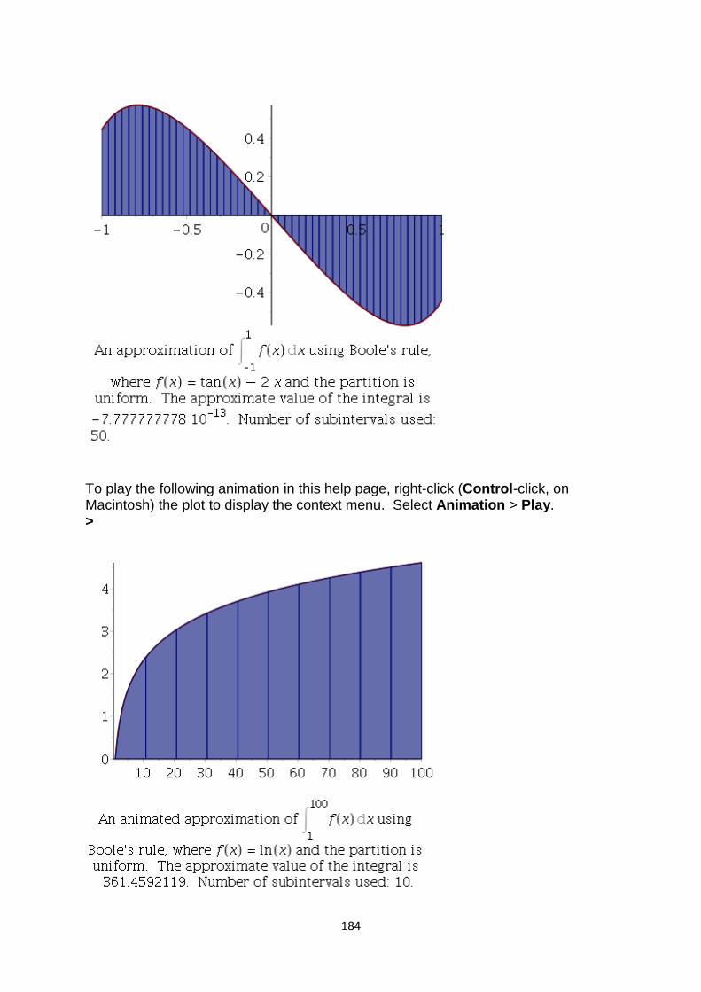
184

To play the following animation in this help page, right-click (Control-click, on Macintosh) the plot to display the context menu. Select Animation > Play. >

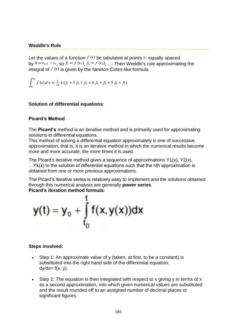
185

Weddle's Rule

Let the values of a function be tabulated at points equally spaced

by , so , , .... Then Weddle's rule approximating the

integral of is given by the Newton-Cotes-like formula

Solution of differential equations:

Picard’s Method The Picard’s method is an iterative method and is primarily used for approximating solutions to differential equations. This method of solving a differential equation approximately is one of successive approximation; that is, it is an iterative method in which the numerical results become more and more accurate, the more times it is used.

The Picard‘s iterative method gives a sequence of approximations Y1(x), Y2(x), …Yk(x) to the solution of differential equations such that the nth approximation is obtained from one or more previous approximations.

The Picard‘s iterative series is relatively easy to implement and the solutions obtained through this numerical analysis are generally power series. Picard’s iteration method formula:

Steps involved: Step 1: An approximate value of y (taken, at first, to be a constant) is

substituted into the right hand side of the differential equation: dy/dx= f(x, y).

Step 2: The equation is then integrated with respect to x giving y in terms of x as a second approximation, into which given numerical values are substituted and the result rounded off to an assigned number of decimal places or significant figures.

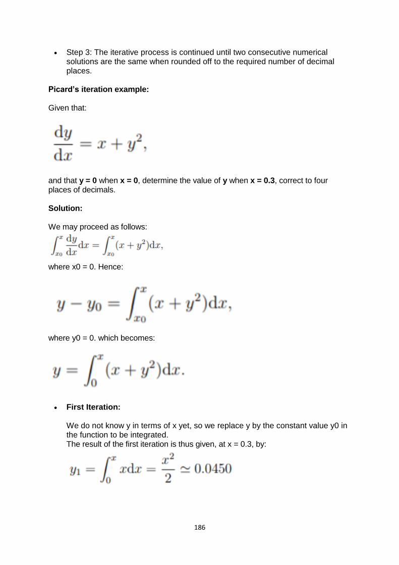
186

Step 3: The iterative process is continued until two consecutive numerical solutions are the same when rounded off to the required number of decimal places.

Picard’s iteration example: Given that:

and that y = 0 when x = 0, determine the value of y when x = 0.3, correct to four places of decimals. Solution: We may proceed as follows:

where x0 = 0. Hence:

where y0 = 0. which becomes:

First Iteration:

We do not know y in terms of x yet, so we replace y by the constant value y0 in the function to be integrated. The result of the first iteration is thus given, at x = 0.3, by:

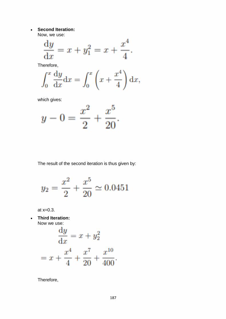
187

Second Iteration: Now, we use:

Therefore,

which gives:

The result of the second iteration is thus given by:

at x=0.3.

Third Iteration: Now we use:

Therefore,

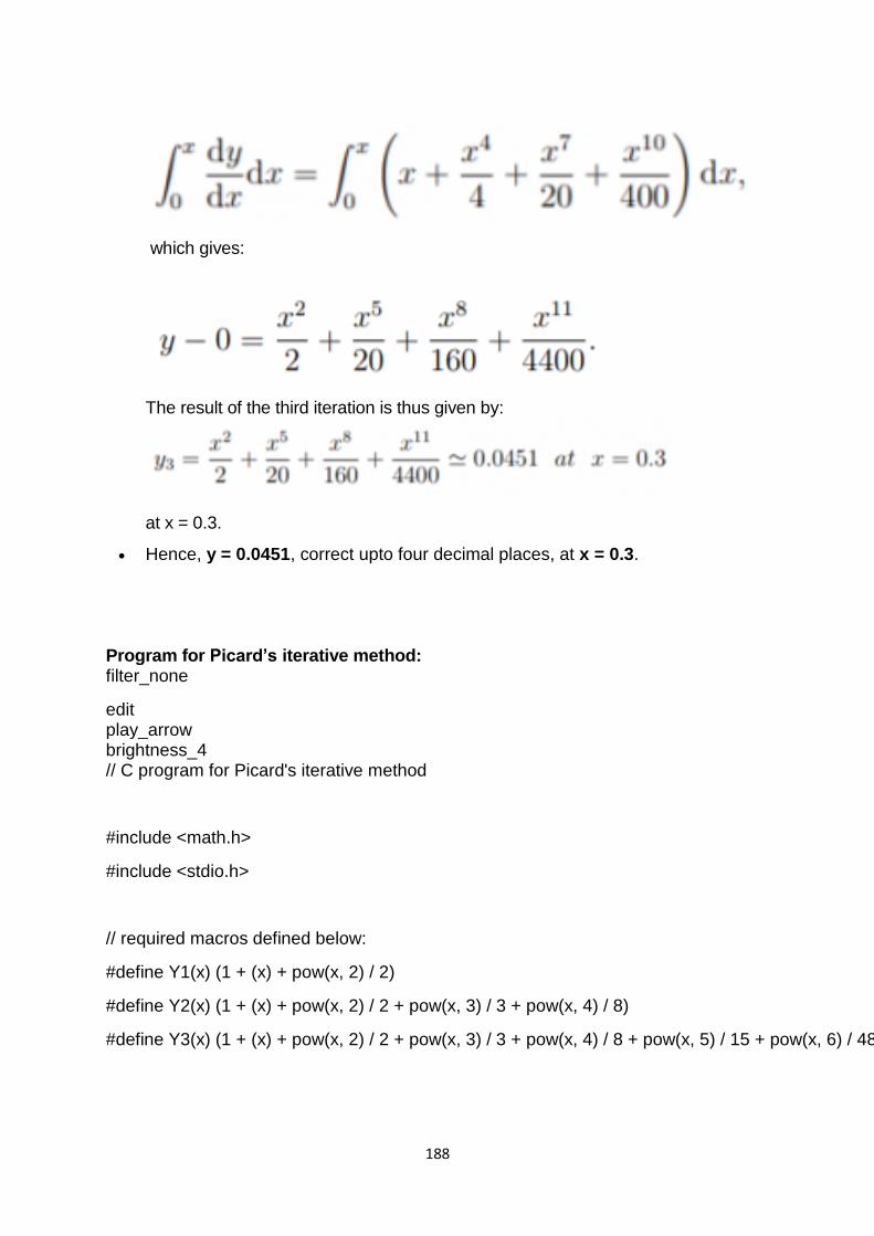
188

which gives:

The result of the third iteration is thus given by:

at x = 0.3.

Hence, y = 0.0451, correct upto four decimal places, at x = 0.3.

Program for Picard’s iterative method: filter_none

edit play_arrow brightness_4 // C program for Picard's iterative method

#include <math.h>

#include <stdio.h>

// required macros defined below:

#define Y1(x) (1 + (x) + pow(x, 2) / 2)

#define Y2(x) (1 + (x) + pow(x, 2) / 2 + pow(x, 3) / 3 + pow(x, 4) / 8)

#define Y3(x) (1 + (x) + pow(x, 2) / 2 + pow(x, 3) / 3 + pow(x, 4) / 8 + pow(x, 5) / 15 + pow(x, 6) / 48)

189

intmain()

{

doublestart_value = 0, end_value = 3,

allowed_error = 0.4, temp;

doubley1[30], y2[30], y3[30];

intcount;

for(temp = start_value, count = 0;

temp <= end_value;

temp = temp + allowed_error, count++) {

y1[count] = Y1(temp);

y2[count] = Y2(temp);

y3[count] = Y3(temp);

}

printf("\nX\n");

for(temp = start_value;

temp <= end_value;

temp = temp + allowed_error) {

// considering all values

// upto 4 decimal places.

printf("%.4lf ", temp);

}

printf("\n\nY(1)\n");

for(temp = start_value, count = 0;

temp <= end_value;

temp = temp + allowed_error, count++) {

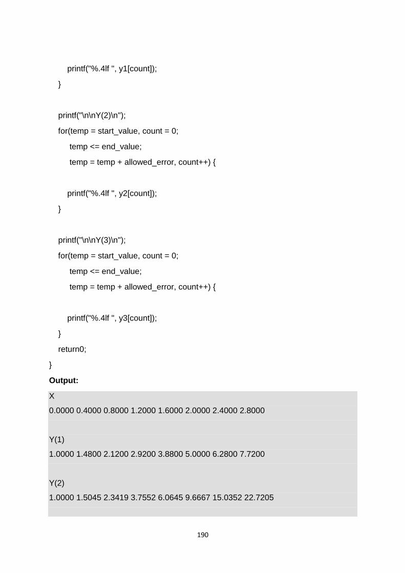
190

printf("%.4lf ", y1[count]);

}

printf("\n\nY(2)\n");

for(temp = start_value, count = 0;

temp <= end_value;

temp = temp + allowed_error, count++) {

printf("%.4lf ", y2[count]);

}

printf("\n\nY(3)\n");

for(temp = start_value, count = 0;

temp <= end_value;

temp = temp + allowed_error, count++) {

printf("%.4lf ", y3[count]);

}

return0;

}

Output:

X

0.0000 0.4000 0.8000 1.2000 1.6000 2.0000 2.4000 2.8000

Y(1)

1.0000 1.4800 2.1200 2.9200 3.8800 5.0000 6.2800 7.7200

Y(2)

1.0000 1.5045 2.3419 3.7552 6.0645 9.6667 15.0352 22.7205

191

Y(3)

1.0000 1.5053 2.3692 3.9833 7.1131 13.1333 24.3249 44.2335

Attention reader! Don‘t stop learning now. Get hold of all the important CS Theory concepts for SDE interviews with the CS Theory Course at a student-friendly price and become industry ready. Euler method

In mathematics and computational science, the Euler method (also called forward Euler method) is a first-order numerical procedure for solving ordinary differential equations (ODEs) with a given initial value. It is the most basic explicit method for numerical integration of ordinary differential equations and is the simplest Runge–Kutta method. The Euler method is named after Leonhard Euler, who treated it in his book Institutionum calculi integralis (published 1768–1870).[1]

The Euler method is a first-order method, which means that the local error (error per step) is proportional to the square of the step size, and the global error (error at a given time) is proportional to the step size. The Euler method often serves as the basis to construct more complex methods, e.g., predictor–corrector method.

Euler‘s Method: If we truncate the Taylor series at the first term y(t + ∆t) = y(t)+∆ty0 (t) + 1 2 ∆t 2 y00(τ ), we can rearrange this and solve for y0 (t) y0 (t) = y(t + ∆t) − y(t) ∆t + O(∆t). Now we can attempt to solve (1.1) by replacing the derivative with a difference: y((n + 1)∆t) ≈ y(n∆t)+∆tf(n∆t, y(n∆t)) Start with y(0) and step forward to solve for any time. What‘s good about this? If the O term is something nice looking, this quantity decays with ∆t, so if we take ∆t smaller and smaller, this gets closer and closer to the real value. What can go wrong? The O term may be ugly. The errors can accumulate as I step forward 1 in time. Also, even though this may be a good approximation for y0 (t) it may not converge to the right solution. To answer these questions, we look at this scheme in depth. Terminology: From now on, we‘ll call yn the numerical approximation to the solution y(n∆t); tn = n∆t. Euler‘s method can then be written yn+1 = yn + ∆tf(tn, yn) n = 1, ..., N − 1 (1.2) This method assumes that you can move from one location to the next using the slope given by the equation (1.1). We saw last time that when we do this, our errors will decay linearly with ∆t. We will show this again today, but in two steps, so that we can generalize it. The proof should look very familiar! Local Truncation Error: To be able to evaluate what we expect the order of a method to look like, we look at the LT E(t) = y(t + ∆t) − y(t) ∆t − f(t, y(t)), i.e. it is the residue when the exact solution of the ODE (1.1) is plugged into the numerical scheme. If yn is close to y(tn) then the LTE will be close to zero. The local truncation error represents the terms neglected by truncating the Taylor series. This is not the error that we get from the method, (i.e. the difference between the real solution and the numerical solution) but will be connected. If I don‘t know y(t), what is the use of this definition? (and if I do know y(t), what do I need the method for?!). It turns out that even without explicit knowledge of the solution we can still calculate the LTE and use it as an estimate and control of the error, by placing certain smoothness assumptions on y(t) and using the Taylor Expansions. Clearly, at time tn, Euler‘s method has Local Truncation Error: LT E = y(tn + ∆t) − y(tn) ∆t − f(tn, y(tn)) = O(∆t), in other words, we can write this y(tn+1) = y(tn)+∆tf(tn, y(tn)) + ∆tLT E. Of course, the method is yn+1 = y(tn)+∆tf(tn, yn). Subtract these two, |y(tn+1) − yn+1| = |y(tn) − yn + ∆t(f(tn, y(tn)) − f(tn, yn)) + ∆tLT E| ≤ |y(tn) − yn| + ∆t|f(tn, y(tn)) −

192

f(tn, yn)| + ∆t|LT E| ≤ |y(tn) − yn| + ∆tL|y(tn) − yn| + ∆t|LT E| . Because f is Lipschitz continuous, | f(tn, y(tn)) − f(tn, yn) y(tn) − yn | ≤ L. 2 And so, if we let the Global Error be en = |y(tn) − yn|, then we can bound the growth of this error: en+1 ≤ en(1 + ∆tL) + LT E∆t. How does this help us bound the method? Lemma: If zi+1 ≤ zi(1 + a∆t) + b Then zi ≤ eai∆t (z0 + b a∆t) Proof: zi+1 ≤ zi (1 + a∆t) + b ≤ (zi−1(1 + a∆t) + b)(1 + a∆t) + b · · · ≤ z0(1 + a∆t) i+1 + b(1 + (1 + a∆t)... + (1 + a∆t) i ) = z0(1 + a∆t) i+1 + b (1 + a∆t)i+1 − 1 1 + a∆t − 1 ≤ z0(1 + a∆t) i+1 + b a∆t (1 + a∆t) i+1 ≤ (1 + a∆t) i+1 z0 + b a∆t ! ≤ ea∆t(i+1) z0 + b a∆t ! so zi ≤ eai∆t (z0 + b a∆t ) Applying this lemma to the global error, we have |en| ≤ eLn∆t (|e0| + M 2L∆t) Now, if n∆t ≤ T then |en| ≤ eLT (|e0| + M 2L∆t) and since |e0| = 0 we have: |en| ≤ eLT ( M 2L ∆t). Compare this with the local error: LT E ≤ 1 2M∆t we see that the global error has the same order as the local error with a different coefficient in the estimates. They are related by the Lipschitz constant L and the final time T. The Order of a scheme r, is defined by |en| = O(∆t r). The higher the order of the scheme, the faster the error decays. Comment: The important thing to understand is that the Local Truncation Error is not always an indicator of what the global error will do. Schemes that have the same order of LTE and global error are good schemes. We need to define what makes the method have the property that the global error will be of same order as the LTE.

Taylor's Series method

Consider the one dimensional initial value problem

y' = f(x, y), y(x0) = y0

where

f is a function of two variables x and y and (x0 , y0) is a known point on the solution

curve.

If the existence of all higher order partial derivatives is assumed for y at x = x0, then by Taylor series the value of y at any neibhouring point x+h can be written as

y(x0+h) = y(x0) + h y'(x0) + h2 /2 y''(x0) + h3/3! y'''(x0) + . . . . . .

where ' represents the derivative with respect to x. Since at x0, y0 is known, y' at x0 can be found by computing f(x0,y0). Similarly higher derivatives of y at x0 also can be computed by making use of the relation y' = f(x,y)

y'' = fx + fyy' y''' = fxx + 2fxyy' + fyy y'2 + fyy''

and so on. Then

y(x0+h) = y(x0) + h f + h2 ( fx + fyy' ) / 2! + h3 ( fxx + 2fxyy' + fyy y'2 + fyy'' ) / 3! + o(h4)

Hence the value of y at any neighboring point x0+ h can be obtained by summing the above infinite series. However, in any practical computation, the summation has to be terminated after some finite number of terms. If the series has been terminated after the pthderivative term then the approximated formula is called the

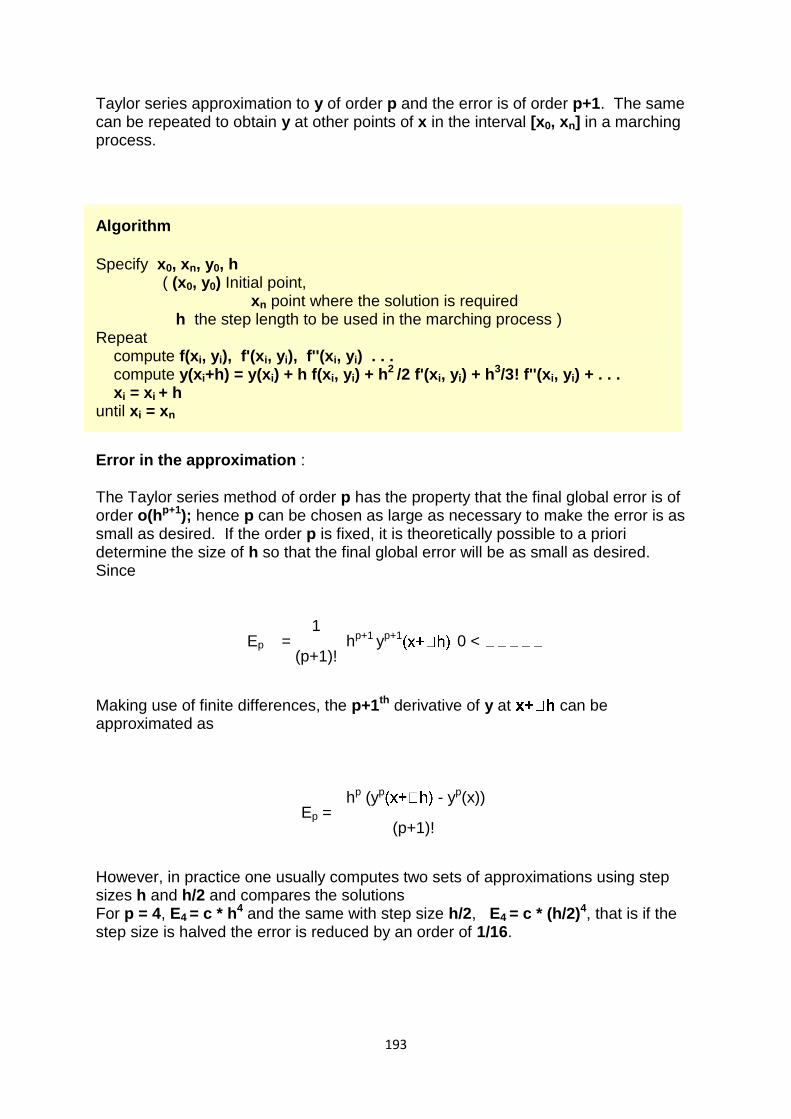
193

Taylor series approximation to y of order p and the error is of order p+1. The same can be repeated to obtain y at other points of x in the interval [x0, xn] in a marching process.

Algorithm

Specify x0, xn, y0, h ( (x0, y0) Initial point, xn point where the solution is required h the step length to be used in the marching process ) Repeat compute f(xi, yi), f'(xi, yi), f''(xi, yi) . . . compute y(xi+h) = y(xi) + h f(xi, yi) + h2 /2 f'(xi, yi) + h3/3! f''(xi, yi) + . . . xi = xi + h until xi = xn

Error in the approximation :

The Taylor series method of order p has the property that the final global error is of order o(hp+1); hence p can be chosen as large as necessary to make the error is as small as desired. If the order p is fixed, it is theoretically possible to a priori determine the size of h so that the final global error will be as small as desired. Since

Ep = 1

hp+1 yp+1 0 < (p+1)!

Making use of finite differences, the p+1th derivative of y at can be approximated as

Ep = hp (yp - yp(x))

(p+1)!

However, in practice one usually computes two sets of approximations using step sizes h and h/2 and compares the solutions For p = 4, E4 = c * h4 and the same with step size h/2, E4 = c * (h/2)4, that is if the step size is halved the error is reduced by an order of 1/16.

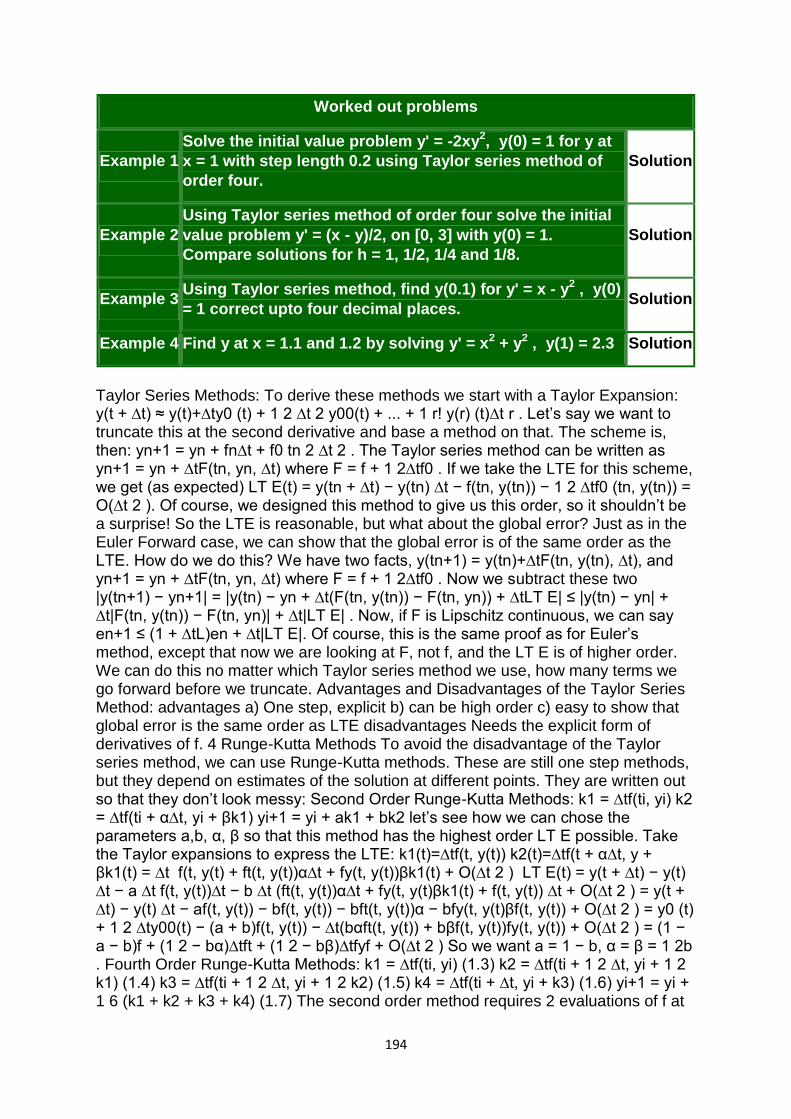
194

Worked out problems

Example 1

Solve the initial value problem y' = -2xy2, y(0) = 1 for y at

x = 1 with step length 0.2 using Taylor series method of

order four.

Solution

Example 2

Using Taylor series method of order four solve the initial

value problem y' = (x - y)/2, on [0, 3] with y(0) = 1.

Compare solutions for h = 1, 1/2, 1/4 and 1/8.

Solution

Example 3 Using Taylor series method, find y(0.1) for y' = x - y2 , y(0)

= 1 correct upto four decimal places. Solution

Example 4 Find y at x = 1.1 and 1.2 by solving y' = x2 + y2 , y(1) = 2.3 Solution

Taylor Series Methods: To derive these methods we start with a Taylor Expansion: y(t + ∆t) ≈ y(t)+∆ty0 (t) + 1 2 ∆t 2 y00(t) + ... + 1 r! y(r) (t)∆t r . Let‘s say we want to truncate this at the second derivative and base a method on that. The scheme is, then: yn+1 = yn + fn∆t + f0 tn 2 ∆t 2 . The Taylor series method can be written as yn+1 = yn + ∆tF(tn, yn, ∆t) where F = f + 1 2∆tf0 . If we take the LTE for this scheme, we get (as expected) LT E(t) = y(tn + ∆t) − y(tn) ∆t − f(tn, y(tn)) − 1 2 ∆tf0 (tn, y(tn)) = O(∆t 2 ). Of course, we designed this method to give us this order, so it shouldn‘t be a surprise! So the LTE is reasonable, but what about the global error? Just as in the Euler Forward case, we can show that the global error is of the same order as the LTE. How do we do this? We have two facts, y(tn+1) = y(tn)+∆tF(tn, y(tn), ∆t), and yn+1 = yn + ∆tF(tn, yn, ∆t) where F = f + 1 2∆tf0 . Now we subtract these two |y(tn+1) − yn+1| = |y(tn) − yn + ∆t(F(tn, y(tn)) − F(tn, yn)) + ∆tLT E| ≤ |y(tn) − yn| + ∆t|F(tn, y(tn)) − F(tn, yn)| + ∆t|LT E| . Now, if F is Lipschitz continuous, we can say en+1 ≤ (1 + ∆tL)en + ∆t|LT E|. Of course, this is the same proof as for Euler‘s method, except that now we are looking at F, not f, and the LT E is of higher order. We can do this no matter which Taylor series method we use, how many terms we go forward before we truncate. Advantages and Disadvantages of the Taylor Series Method: advantages a) One step, explicit b) can be high order c) easy to show that global error is the same order as LTE disadvantages Needs the explicit form of derivatives of f. 4 Runge-Kutta Methods To avoid the disadvantage of the Taylor series method, we can use Runge-Kutta methods. These are still one step methods, but they depend on estimates of the solution at different points. They are written out so that they don‘t look messy: Second Order Runge-Kutta Methods: k1 = ∆tf(ti, yi) k2 = ∆tf(ti + α∆t, yi + βk1) yi+1 = yi + ak1 + bk2 let‘s see how we can chose the parameters a,b, α, β so that this method has the highest order LT E possible. Take the Taylor expansions to express the LTE: k1(t)=∆tf(t, y(t)) k2(t)=∆tf(t + α∆t, y + βk1(t) = ∆t f(t, y(t) + ft(t, y(t))α∆t + fy(t, y(t))βk1(t) + O(∆t 2 ) LT E(t) = y(t + ∆t) − y(t) ∆t − a ∆t f(t, y(t))∆t − b ∆t (ft(t, y(t))α∆t + fy(t, y(t)βk1(t) + f(t, y(t)) ∆t + O(∆t 2 ) = y(t + ∆t) − y(t) ∆t − af(t, y(t)) − bf(t, y(t)) − bft(t, y(t))α − bfy(t, y(t)βf(t, y(t)) + O(∆t 2 ) = y0 (t) + 1 2 ∆ty00(t) − (a + b)f(t, y(t)) − ∆t(bαft(t, y(t)) + bβf(t, y(t))fy(t, y(t)) + O(∆t 2 ) = (1 − a − b)f + (1 2 − bα)∆tft + (1 2 − bβ)∆tfyf + O(∆t 2 ) So we want a = 1 − b, α = β = 1 2b . Fourth Order Runge-Kutta Methods: k1 = ∆tf(ti, yi) (1.3) k2 = ∆tf(ti + 1 2 ∆t, yi + 1 2 k1) (1.4) k3 = ∆tf(ti + 1 2 ∆t, yi + 1 2 k2) (1.5) k4 = ∆tf(ti + ∆t, yi + k3) (1.6) yi+1 = yi + 1 6 (k1 + k2 + k3 + k4) (1.7) The second order method requires 2 evaluations of f at

195

every timestep, the fourth order method requires 4 evaluations of f at every timestep. In general: For an rth order RungeKutta method we need S(r) evaluations of f for

7 5 Practically speaking, people stop at r = 5. Advantages of Runge-Kutta Methods 1. One step method – global error is of the same order as local error. 2. Don‘t need to know derivatives of f. 3. Easy for ‖Automatic Error Control‖. Automatic Error Control Uniform grid spacing – in this case, time steps – are good for some cases but not always. Sometimes we deal with problems where varying the gridsize makes sense. How do you know when to change the stepsize? If we have an rth order scheme and and r + 1th order scheme, we can take the difference between these two to be the error in the scheme, and make the stepsize smaller if we prefer a smaller error, or larger if we can tolerate a larger error. For Automatic error control yo are computing a ‖useless‖ (r+1)th order shceme . . . what a waste! But with Runge Kutta we can take a fifth order method and a fourth order method, using the same ks. only a little extra work at each step

Runge-Kutta Method :

Runge-Kutta method here after called as RK method is the generalization of the concept used in Modified Euler's method.

In Modified Eulers method the slope of the solution curve has been approximated with the slopes of the curve at the end points of the each sub interval in computing the solution. The natural generalization of this concept is computing the slope by taking a weighted average of the slopes taken at more number of points in each sub interval. However, the implementation of the scheme differes from Modified Eulers method so that the developed algorithm is explicit in nature. The final form of the scheme is of the form

yi+1 = yi + (weighted average of the slopes) for i = 0, 1, 2 . . . where h is the step length and yi and yi+1 are the values of y at xi and xi+1 respectively.

In genaral, the slope is computed at various points xs in each sub interval [xi, xi+1] and multiplied them with the step length h and then weighted average of it is then added to yi to compute yi+1. Thus the RK method with v slopes called as v-stage RKmethod can be written as

K1 = h f(xi, yi) K2 = h f(xi + c2h, yi + a21K1) K3 = h f(xi + c3h, yi + a31K1+ a32K2) . . . . . . . . .

Kv = h f(xi + cvh, yi + av1K1+ av2K2 + . . . +avv-1Kv-1) and

yi+1 = yi + (W1 K1 + W2 K2 + . . . + Wv Kv ) for i = 0, 1, 2 . . .

196

To determine the parameters c's, a's and W's in the above equation, yi+1 defined in the scheme is expanded interms of steplengh h and the resultant equation is then compared with Taylor series expansion of the solution of the differential equation upto a certain number of terms say p. Then the v-stage RKmethod will be of order p or is an pth order RK method. Here for any v>4 the maximum possible order p of the R Kmethod is always less than v. However, for any v lessthan or equal to 4, it is possible derive an RK method of order p = v. Now, consider the case v = 2 to derive the 2-stage RK method. For this

K1 = h f(xi, yi) K2 = h f(xi + c2h, yi + a21K1) yi+1 = yi + ( W1 K1 + W2 K2 ) for i = 0, 1, 2 . . .

Now by Taylor series expansion

y(xi+1) = y(xi) + h y'(xi) + h2 y''(xi)/2! + h3 y'''(xi)/3! + o(h4) = y(xi) + h f + h2 ( fx + fyf ) / 2! + h3( fxx + 2fxyf + fyy f

2 + fy( fx + fyf )) / 3! + o(h4)

Also

K1 = h fi K2 = h f(xi + c2h, yi + a21K1) = h( fi + c2h fx + a21K1fy + ( c2h)2 fxx /2! + (a21K1)

2 fyy /2! + c2h a21K1 fxy + o(h4) ) = h( fi + c2h fx + a21h fi fy + ( c2h)2 fxx /2! + (a21h fi)

2 fyy /2! + c2h a21h fi fxy + o(h4) ) yi+1 = yi + (W1+W2) h fi + h2(W2c2fx + W2a21f fy) + h3 W2(c2

2a21f fxy + a221f

2 fyy)/2 + o(h4)

Now by comparing the equal powers of h inyi+1and y(xi+1) we get

W1 + W2 = 1 c2W2 = 1/2 and a21W2 = 1/2

The solution of this system is

a21 = c2, W2 = 1/(2c2) and W1 = 1 - 1/(2c2)

where c2 is any arbitrary constant not equal to zero. For these values of a21, W2 , W1, since 2-stage RK method compares with Taylor series upto h2for any value of c2 the 2-stage RK method is of order two and hence this scheme is denoted in many text books as a second order RK method. Now, to give some numerical values to a21, W2 , W1 first the valuec2 of has to be fixed. Generally the value of c2 is fixed such that the values of a21, W2 , W1 are integers or some real numbers which easy to remember. Two of such cases are c2 = 1/2 and c2=1.

Case (i): c2 = 1/2 a21= 1/2, W2 = 1, W1 = 0. The corresopnding 2-stage (second order) RK method is

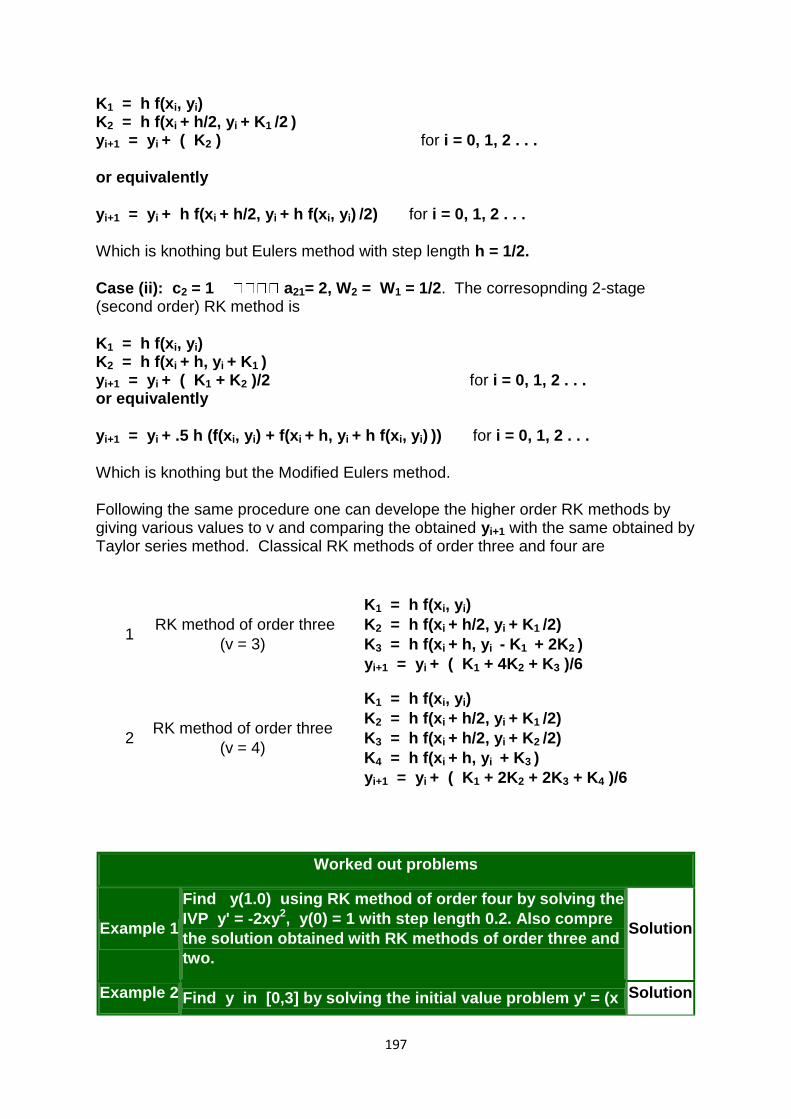
197

K1 = h f(xi, yi) K2 = h f(xi + h/2, yi + K1 /2 ) yi+1 = yi + ( K2 ) for i = 0, 1, 2 . . .

or equivalently

yi+1 = yi + h f(xi + h/2, yi + h f(xi, yi) /2) for i = 0, 1, 2 . . .

Which is knothing but Eulers method with step length h = 1/2.

Case (ii): c2 = 1 a21= 2, W2 = W1 = 1/2. The corresopnding 2-stage (second order) RK method is

K1 = h f(xi, yi) K2 = h f(xi + h, yi + K1 ) yi+1 = yi + ( K1 + K2 )/2 for i = 0, 1, 2 . . . or equivalently

yi+1 = yi + .5 h (f(xi, yi) + f(xi + h, yi + h f(xi, yi) )) for i = 0, 1, 2 . . .

Which is knothing but the Modified Eulers method.

Following the same procedure one can develope the higher order RK methods by giving various values to v and comparing the obtained yi+1 with the same obtained by Taylor series method. Classical RK methods of order three and four are

1 RK method of order three

(v = 3)

K1 = h f(xi, yi)

K2 = h f(xi + h/2, yi + K1 /2)

K3 = h f(xi + h, yi - K1 + 2K2 )

yi+1 = yi + ( K1 + 4K2 + K3 )/6

2 RK method of order three

(v = 4)

K1 = h f(xi, yi)

K2 = h f(xi + h/2, yi + K1 /2)

K3 = h f(xi + h/2, yi + K2 /2)

K4 = h f(xi + h, yi + K3 )

yi+1 = yi + ( K1 + 2K2 + 2K3 + K4 )/6

Worked out problems

Example 1

Find y(1.0) using RK method of order four by solving the

IVP y' = -2xy2, y(0) = 1 with step length 0.2. Also compre

the solution obtained with RK methods of order three and

two.

Solution

Example 2 Find y in [0,3] by solving the initial value problem y' = (x Solution

198

- y)/2, y(0) = 1 using RK method of order four with h = 1/2

and 1/4.

Example 3 Using RK method of order four find y(0.1) for y' = x - y2,

y(0) = 1. Solution

Example 4 Using RK method of order four find y at x = 1.1 and 1.2 by

solving y' = x2 + y2 , y(1) = 2.3 Solution

Runge-Kutta Methods

In the forward Euler method, we used the information on the slope or the derivative

of y at the given time step to extrapolate the solution to the next time-step. The LTE

for the method is O(h2), resulting in a first order numerical technique. Runge-Kutta

methods are a class of methods which judiciously uses the information on the 'slope'

at more than one point to extrapolate the solution to the future time step. Let's

discuss first the derivation of the second order RK method where the LTE is O(h3).

Given the IVP of Eq. 6, and a time step h, and the solution yn at the nth time step, let's say that we wish to compute yn+1 in the following fashion:

k1 = hf(yn,tn)

yn+1 = yn + ak1 + bk2, (12)

where the constants , , a and b have to be evaluated so that the resulting

method has a LTE O(h3). Note that if k2=0 and a=1, then Eq. 13 reduces to the

forward Euler method.

Now, let's write down the Taylor series expansion of y in the neighborhood of tn correct to the h2 term i.e.,

(13)

199

However, we know from the IVP (Eq. 6) that dy/dt = f(y,t) so that

(14)

So from the above analysis, i.e., Eqs. 14 and 15, we get

(15)

However, the term k2 in the proposed RK method of Eq. 13 can be expanded correct

to O(h3) as

(16)

Now, substituting for k2 from Eq. 17 in Eq. 13, we get

(17)

Comparing the terms with identical coefficients in Eqs. 16 and 18 gives us the following system of equations to determine the constants:

a+b=1

200

(18)

There are infinitely many choices of a, b, and which satisfy Eq. 19, we can

choose for instance and a=b=1/2. With this choice, we have the

classical second order accurate Runge-Kutta method (RK2) which is summarized as

follows.

k1 = hf(yn,tn)

k2 = hf(yn+k1, tn + h)

(19

)

In a similar fashion Runge-Kutta methods of higher order can be developed. One of the most widely used methods for the solution of IVPs is the fourth order Runge-Kutta (RK4) technique. The LTE of this method is order h5. The method is given below.

k1 = hf(yn,tn)

k2 = hf(yn+k1/2, tn + h/2)

k4 = h(yn+k3, tn + h)

yn+1 = yn + (k1 + 2k2 + 2k3 + k4)/6.

Last Updated: 16-09-2019

For a given differential equation with initial

condition find the approximate solution using Predictor-Corrector method.

Predictor-Corrector Method : The predictor-corrector method is also known as Modified-Euler method. In the Euler method, the tangent is drawn at a point and slope is calculated for a given step size. Thus this method works best with linear functions, but for other cases, there

201

remains a truncation error. To solve this problem the Modified Euler method is introduced. In this method instead of a point, the arithmetic average of the slope over an interval is used. Thus in the Predictor-Corrector method for each step the predicted value of is calculated first using Euler‘s method and then the slopes at the points and is calculated and the arithmetic average of these slopes are added to to calculate the

corrected value of .

As, in this method, the average slope is used, so the error is reduced significantly. Also, we can repeat the process of correction for convergence. Thus at every step, we are reducing the error thus by improving the value of y.

Examples:

Input : eq = , y(0) = 0.5, step size(h) = 0.2 To find: y(1) Output: y(1) = 2.18147 Explanation: The final value of y at x = 1 is y=2.18147 Implementation: Here we are considering the differential

equation:

C++

Java

Python3

C#

PHP

filter_none

edit

play_arrow

brightness_4 // C++ code for solving the differential equation

// using Predictor-Corrector or Modified-Euler method

// with the given conditions, y(0) = 0.5, step size(h) = 0.2

// to find y(1)

#include <bits/stdc++.h>

usingnamespacestd;

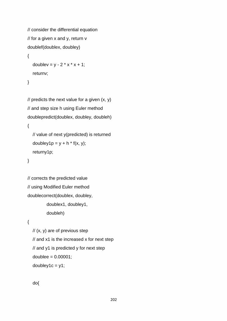
202

// consider the differential equation

// for a given x and y, return v

doublef(doublex, doubley)

{

doublev = y - 2 * x * x + 1;

returnv;

}

// predicts the next value for a given (x, y)

// and step size h using Euler method

doublepredict(doublex, doubley, doubleh)

{

// value of next y(predicted) is returned

doubley1p = y + h * f(x, y);

returny1p;

}

// corrects the predicted value

// using Modified Euler method

doublecorrect(doublex, doubley,

doublex1, doubley1,

doubleh)

{

// (x, y) are of previous step

// and x1 is the increased x for next step

// and y1 is predicted y for next step

doublee = 0.00001;

doubley1c = y1;

do{

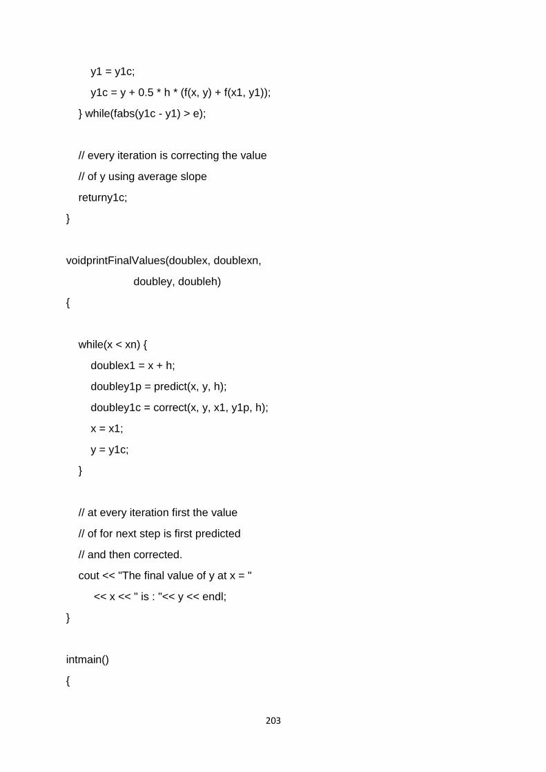
203

y1 = y1c;

y1c = y + 0.5 * h * (f(x, y) + f(x1, y1));

} while(fabs(y1c - y1) > e);

// every iteration is correcting the value

// of y using average slope

returny1c;

}

voidprintFinalValues(doublex, doublexn,

doubley, doubleh)

{

while(x < xn) {

doublex1 = x + h;

doubley1p = predict(x, y, h);

doubley1c = correct(x, y, x1, y1p, h);

x = x1;

y = y1c;

}

// at every iteration first the value

// of for next step is first predicted

// and then corrected.

cout << "The final value of y at x = "

<< x << " is : "<< y << endl;

}

intmain()

{

204

// here x and y are the initial

// given condition, so x=0 and y=0.5

doublex = 0, y = 0.5;

// final value of x for which y is needed

doublexn = 1;

// step size

doubleh = 0.2;

printFinalValues(x, xn, y, h);

return0;

}

AUTOMATIC ERROR MONITORING

Exception/Error Monitoring is a process to monitor the log files generated by the applications, events, and services to identify the errors or exceptions occurred in the applications running. Exception/Error Monitoring helps in identifying the errors by scanning the log files for specific keyword/text pattern and generate alerts to notify the user.

Serious errors like OutOfMemoryError get logged into server's log files which makes server not perform its usual operations in desired manner even though it continues to run. The Exception/Error monitor will watch your server's log files and alert you as soon as it finds pre-configured search conditions.

This tutorial provides a brief introduction on monitoring Log files using AgentlessMonitor. This tutorial assumes that you have successfully installed AgentlessMonitor.

Configuring Agentless Monitor to monitor Exception/Error in log files

Following steps will explain how you can configure AppPerfect Agentless Monitor for Exception/Error Monitoring :

o Once you are logged into the Monitor Server you can see the Web-UI from which you can access all the features of the Monitor Server. Click the Monitors link from the left sidebar. This will take you to Monitors tab. Click on Add button to Add a New Exception/Error Monitor.

205

o Next Step is to define the Exception/Error Monitor. Provide the IP Address or Host Name of the system whose log files need to be monitored.

o Select the monitor type as Exception/Error Monitor to monitor Logs for errors or exceptions.

o Specify a meaningful identifier for the monitor which will help identify the monitor in future. AppPerfect also supports legacy agent-based architecture. In case you need to use agent-based monitoring, AppPerfect can provide agent for monitoring remote machine, in which case it requires the agent to be deployed on remote machine running at a specific port.

o Specify the Data Fetch Interval which represents the time interval for which application should wait before fetching the monitoring data from the device. Monitoring Data will be fetched after every specified fetch interval. The smaller the time interval, the more granular the data. However, smaller time intervals also result in a much larger data set.

o You can specify if the monitor should be Active as soon as its added or should it be in suspended state. You can also specify if all the attributes should be monitored or only some predefined attributes should be monitored.

o Next Option is to provide server specific configuration settings. Provide the log file(s) you want to monitor, message pattern and user credentials. You can add some keywords to the whitelist, so the monitor will ignore those patterns while monitoring. Once you are done providing the server settings, click on Validate Connection button to confirm that the specified log file(s) on the server is accessible.

o Next Step is to Select the Attributes to monitor. Exception/Error Monitoring allows you to monitor the parameters such as lines read, exception summary, match count etc. Select the parameters you need to monitor from the list of attributes shown.

o Next step shows the Attribute details of all the selected attributes in the previous step. You can customize the display labels for each of the attributes here. You can change the label for time from milliseconds to microseconds.

o Next step shows the Attribute Data conversion where you can convert the attribute value to required unit. You can configure the operation which should be performed on the attribute value to create the final output value.

o Next step shows the Defining Rules view. This view will provide a list of all numeric attributes. You can select the attributes for which you want to add a rule. A rule is defined as a conditional or threshold value which when exceeds, a notification would be sent. In a typical workflow the monitors

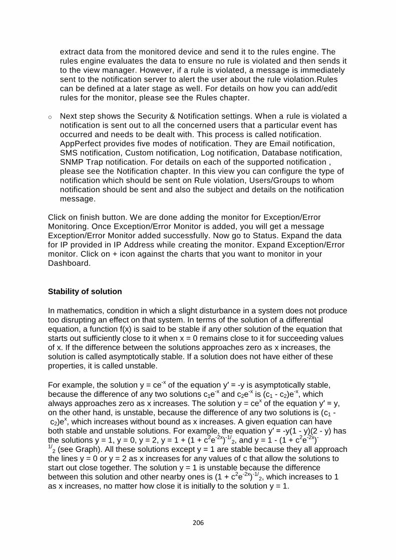
206

extract data from the monitored device and send it to the rules engine. The rules engine evaluates the data to ensure no rule is violated and then sends it to the view manager. However, if a rule is violated, a message is immediately sent to the notification server to alert the user about the rule violation.Rules can be defined at a later stage as well. For details on how you can add/edit rules for the monitor, please see the Rules chapter.

o Next step shows the Security & Notification settings. When a rule is violated a notification is sent out to all the concerned users that a particular event has occurred and needs to be dealt with. This process is called notification. AppPerfect provides five modes of notification. They are Email notification, SMS notification, Custom notification, Log notification, Database notification, SNMP Trap notification. For details on each of the supported notification , please see the Notification chapter. In this view you can configure the type of notification which should be sent on Rule violation, Users/Groups to whom notification should be sent and also the subject and details on the notification message.

Click on finish button. We are done adding the monitor for Exception/Error Monitoring. Once Exception/Error Monitor is added, you will get a message Exception/Error Monitor added successfully. Now go to Status. Expand the data for IP provided in IP Address while creating the monitor. Expand Exception/Error monitor. Click on + icon against the charts that you want to monitor in your Dashboard.

Stability of solution

In mathematics, condition in which a slight disturbance in a system does not produce too disrupting an effect on that system. In terms of the solution of a differential equation, a function f(x) is said to be stable if any other solution of the equation that starts out sufficiently close to it when x = 0 remains close to it for succeeding values of x. If the difference between the solutions approaches zero as x increases, the solution is called asymptotically stable. If a solution does not have either of these properties, it is called unstable.

For example, the solution y = ce-x of the equation y′ = -y is asymptotically stable, because the difference of any two solutions c1e

-x and c2e-x is (c1 - c2)e

-x, which always approaches zero as x increases. The solution y = cex of the equation y′ = y, on the other hand, is unstable, because the difference of any two solutions is (c1 - c2)e

x, which increases without bound as x increases. A given equation can have both stable and unstable solutions. For example, the equation y′ = -y(1 - y)(2 - y) has the solutions y = 1, y = 0, y = 2, y = 1 + (1 + c2e-2x)-1/

2, and y = 1 - (1 + c2e-2x)-

1/2 (see Graph). All these solutions except y = 1 are stable because they all approach

the lines y = 0 or y = 2 as x increases for any values of c that allow the solutions to start out close together. The solution y = 1 is unstable because the difference between this solution and other nearby ones is (1 + c2e-2x)-1/

2, which increases to 1 as x increases, no matter how close it is initially to the solution y = 1.

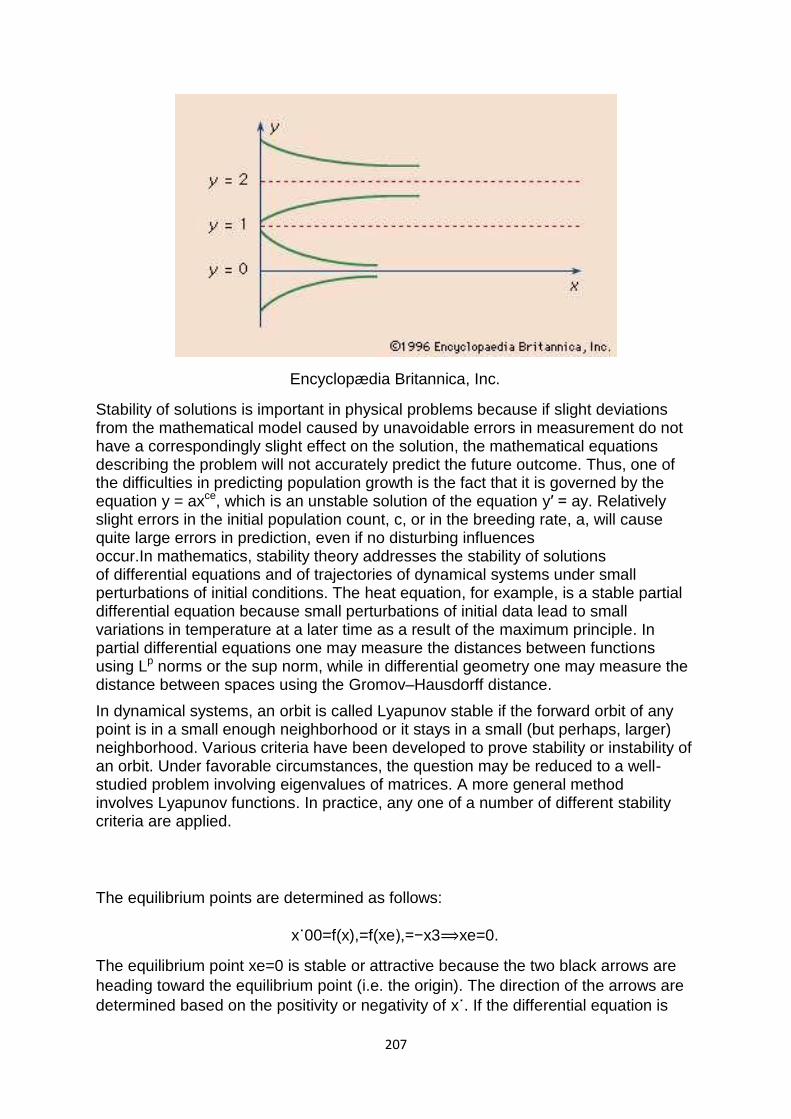
207

Encyclopædia Britannica, Inc.

Stability of solutions is important in physical problems because if slight deviations from the mathematical model caused by unavoidable errors in measurement do not have a correspondingly slight effect on the solution, the mathematical equations describing the problem will not accurately predict the future outcome. Thus, one of the difficulties in predicting population growth is the fact that it is governed by the equation y = axce, which is an unstable solution of the equation y′ = ay. Relatively slight errors in the initial population count, c, or in the breeding rate, a, will cause quite large errors in prediction, even if no disturbing influences occur.In mathematics, stability theory addresses the stability of solutions of differential equations and of trajectories of dynamical systems under small perturbations of initial conditions. The heat equation, for example, is a stable partial differential equation because small perturbations of initial data lead to small variations in temperature at a later time as a result of the maximum principle. In partial differential equations one may measure the distances between functions using Lp norms or the sup norm, while in differential geometry one may measure the distance between spaces using the Gromov–Hausdorff distance.

In dynamical systems, an orbit is called Lyapunov stable if the forward orbit of any point is in a small enough neighborhood or it stays in a small (but perhaps, larger) neighborhood. Various criteria have been developed to prove stability or instability of an orbit. Under favorable circumstances, the question may be reduced to a well-studied problem involving eigenvalues of matrices. A more general method involves Lyapunov functions. In practice, any one of a number of different stability criteria are applied.

The equilibrium points are determined as follows:

x˙00=f(x),=f(xe),=−x3⟹xe=0.

The equilibrium point xe=0 is stable or attractive because the two black arrows are

heading toward the equilibrium point (i.e. the origin). The direction of the arrows are

determined based on the positivity or negativity of x˙. If the differential equation is

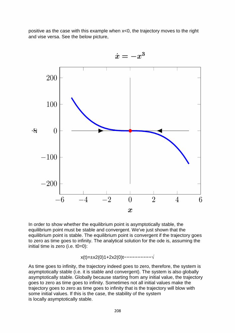
208

positive as the case with this example when x<0, the trajectory moves to the right

and vise versa. See the below picture,

In order to show whether the equilibrium point is asymptotically stable, the equilibrium point must be stable and convergent. We've just shown that the equilibrium point is stable. The equilibrium point is convergent if the trajectory goes to zero as time goes to infinity. The analytical solution for the ode is, assuming the initial time is zero (i.e. t0=0):

x(t)=±x2(0)1+2x2(0)t−−−−−−−−−−√

As time goes to infinity, the trajectory indeed goes to zero, therefore, the system is asymptotically stable (i.e. it is stable and convergent). The system is also globally asymptotically stable. Globally because starting from any initial value, the trajectory goes to zero as time goes to infinity. Sometimes not all initial values make the trajectory goes to zero as time goes to infinity that is the trajectory will blow with some initial values. If this is the case, the stability of the system is locally asymptotically stable.

209