computer graphics cs 3600 scan conversion file– circles: bresenham, 1977 • currently implemented...
TRANSCRIPT
Computer Graphics
CS 3600
Scan Conversion
Rasterization of Primitives
• How to draw primitives?
– Convert from geometric definition to pixels
– rasterization = selecting the pixels
• Will be done frequently
– must be fast:
• use integer arithmetic
• use addition instead of multiplication
Rasterization Algorithms
• Algorithmics:
– Line-drawing: Bresenham, 1965
– Polygons: uses line-drawing
– Circles: Bresenham, 1977
• Currently implemented in all graphics libraries
Point plotting
• Application program furnish the co-ordinates
• If the co-ordinates are real nos, they are rounded off to nearest
integer, as device co-ordinates support only integer co-
ordinates
• On vector scan CRT
– Point plotting instruction stored in the display list
– The instruction set appropriate deflection voltage for the electron bean
to aim it to the screen location
Point plotting
• On raster-scan B/W CRT – The bit value at the corresponding position in the frame buffer is
set to 1
– Electron beam sweeps the screen area (scanning) as per the frame
buffer
– It emits a burst of electron whenever it encounters a 1 in the frame
buffer
• On raster scan color CRT
– Color code + table lookup

Line Scan Conversion
Line Plotting
• Two end points (co-ordinates) are specified
• Intermediate positions between end points are calculated
(using line eqn)
• The intermediate and end points are plotted
• Pixel level color management to draw line on color CRT
Scan Conversion Problem of Lines
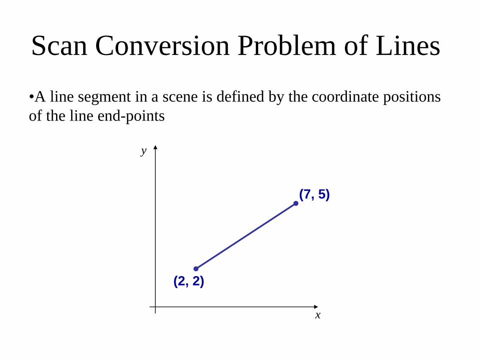
•A line segment in a scene is defined by the coordinate positions
of the line end-points
x
y
(2, 2)
(7, 5)
The Problem (cont…)
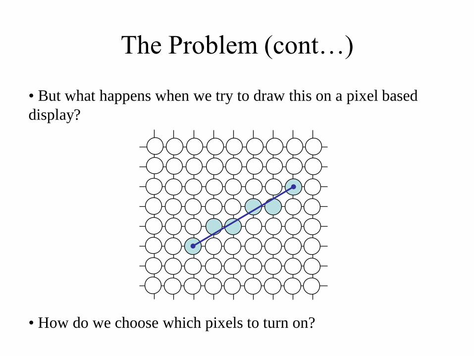
• But what happens when we try to draw this on a pixel based
display?
• How do we choose which pixels to turn on?
Line Plotting
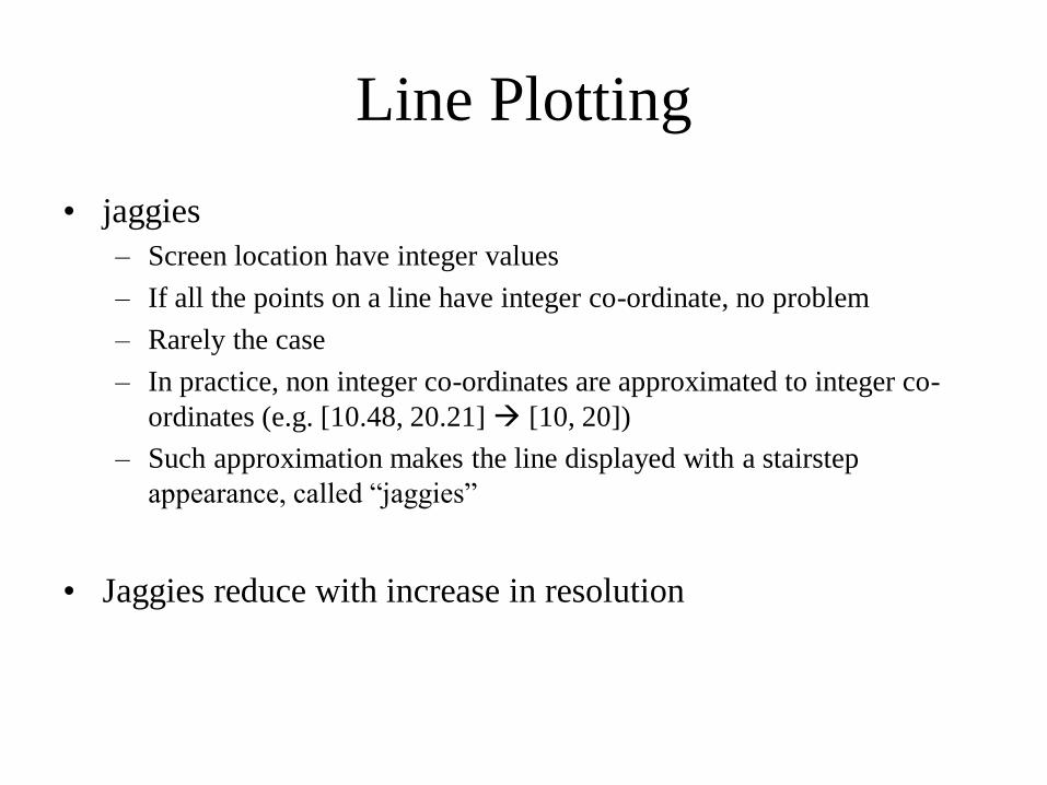
• jaggies
– Screen location have integer values
– If all the points on a line have integer co-ordinate, no problem
– Rarely the case
– In practice, non integer co-ordinates are approximated to integer co-
ordinates (e.g. [10.48, 20.21] [10, 20])
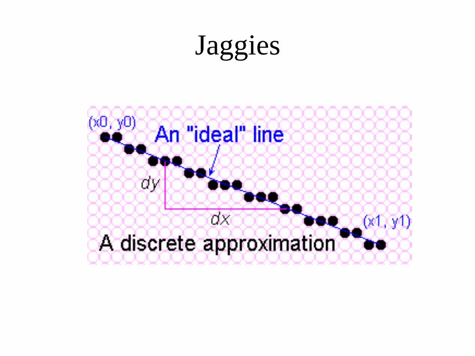
– Such approximation makes the line displayed with a stairstep
appearance, called “jaggies”
• Jaggies reduce with increase in resolution
Jaggies
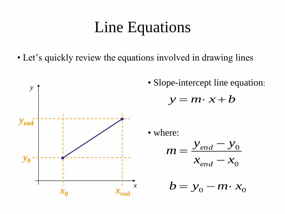
Line Equations
• Let’s quickly review the equations involved in drawing lines
x
y
y0
yend
xend x0
• Slope-intercept line equation:
bxmy
• where:
0
0
xx
yym
end
end
00 xmyb
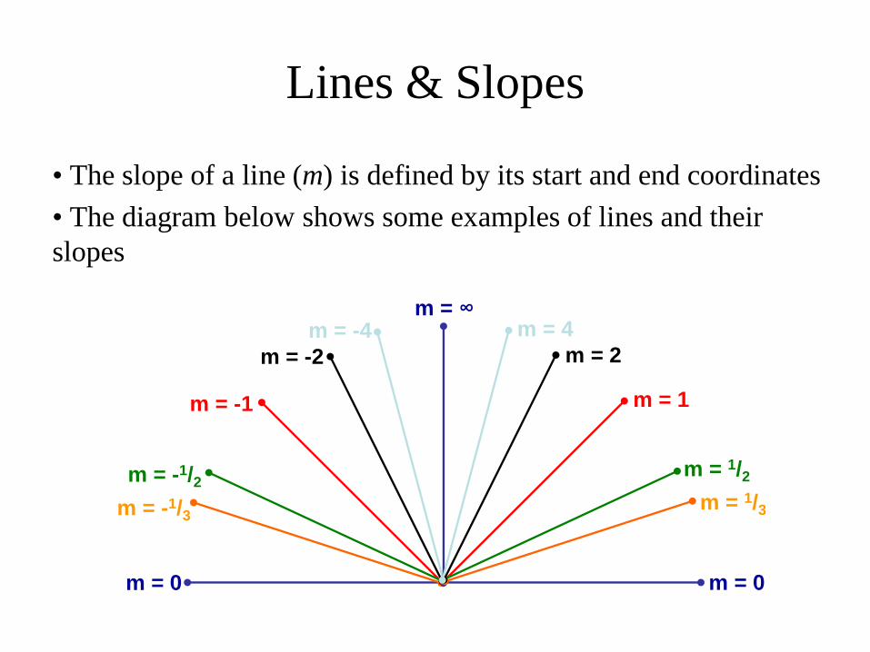
Lines & Slopes
• The slope of a line (m) is defined by its start and end coordinates
• The diagram below shows some examples of lines and their
slopes
m = 0
m = -1/3
m = -1/2
m = -1
m = -2
m = -4
m = ∞
m = 1/3
m = 1/2
m = 1
m = 2
m = 4
m = 0
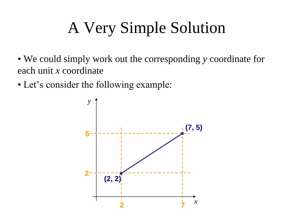
A Very Simple Solution
• We could simply work out the corresponding y coordinate for
each unit x coordinate
• Let’s consider the following example:
x
y
(2, 2)
(7, 5)
2 7
2
5
A Very Simple Solution (cont…)
x
y
(2, 2)
(7, 5)
2 3 4 5 6 7
2
5
5
3
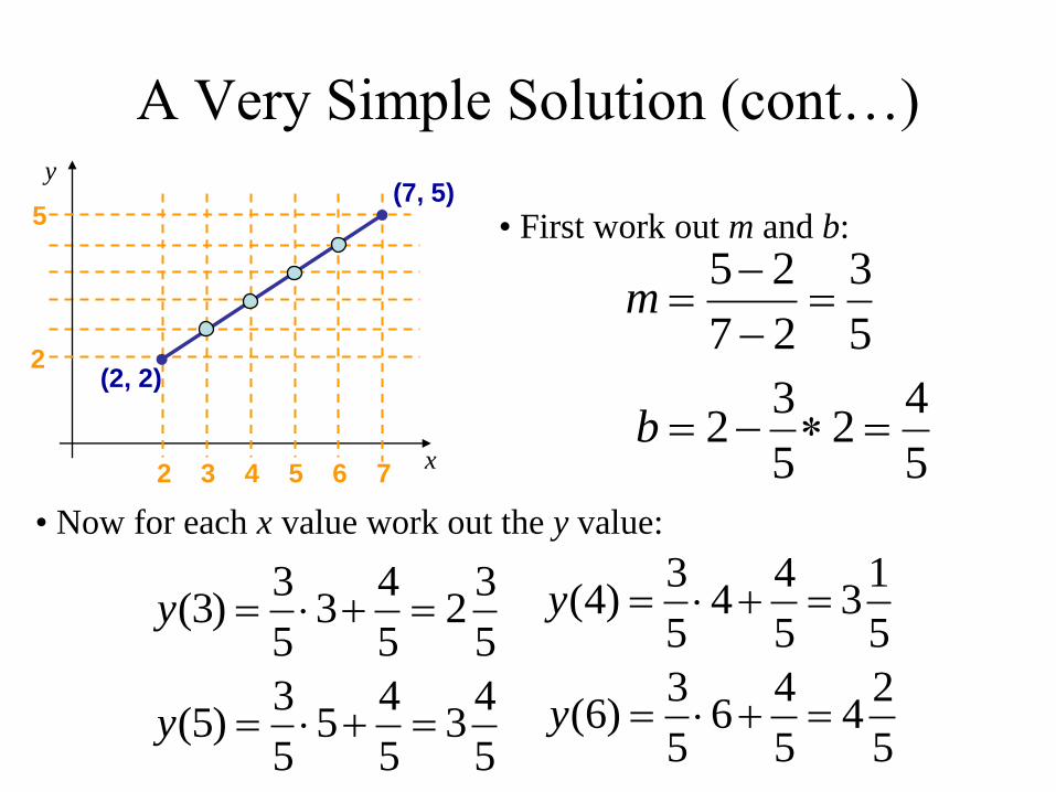
27
25
m
5
42
5
32 b
• First work out m and b:
• Now for each x value work out the y value:
5
32
5
43
5
3)3( y
5
13
5
44
5
3)4( y
5
43
5
45
5
3)5( y
5
24
5
46
5
3)6( y

A Very Simple Solution (cont…)
•Now just round off the results and turn on these pixels to draw
our line
35
32)3( y
35
13)4( y
45
43)5( y
45
24)6( y
0 1 2 3 4 5 6 7 8
0
1
2
3
4
5
6
7
A Very Simple Solution (cont…)
• However, this approach is just way too slow
• In particular look out for:
– The equation y = mx + b requires the multiplication of m by x
– Rounding off the resulting y coordinates
• We need a faster solution
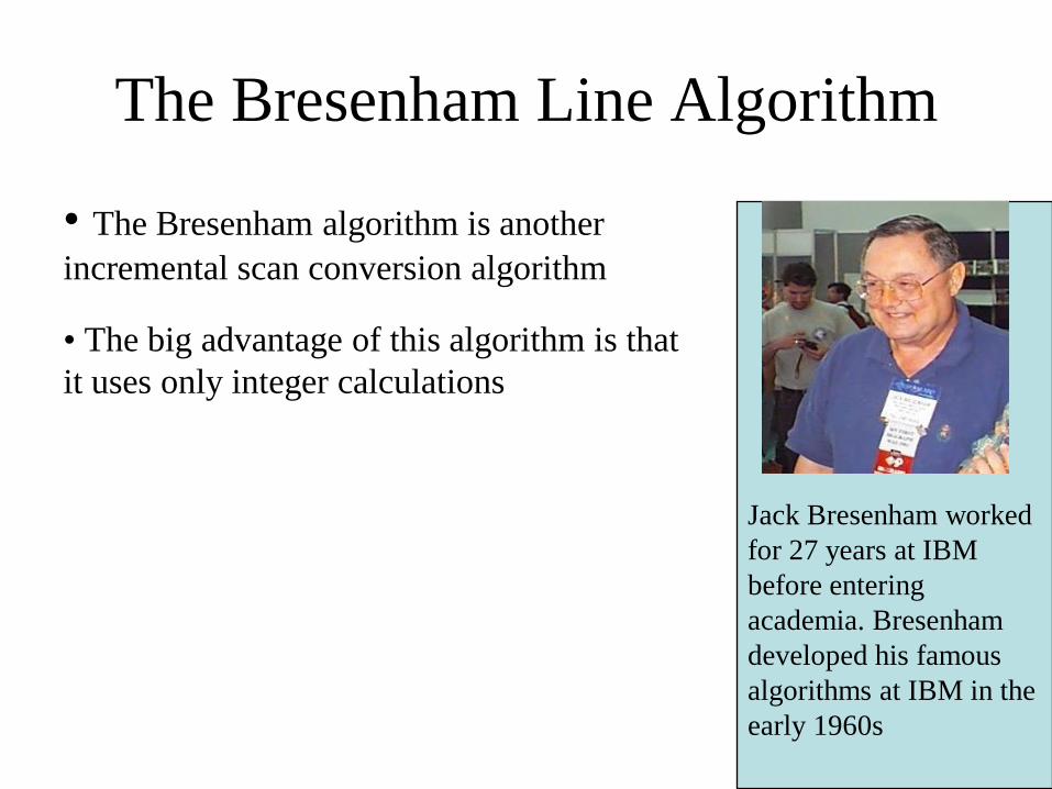
The Bresenham Line Algorithm
• The Bresenham algorithm is another
incremental scan conversion algorithm
• The big advantage of this algorithm is that
it uses only integer calculations
Jack Bresenham worked
for 27 years at IBM
before entering
academia. Bresenham
developed his famous
algorithms at IBM in the
early 1960s
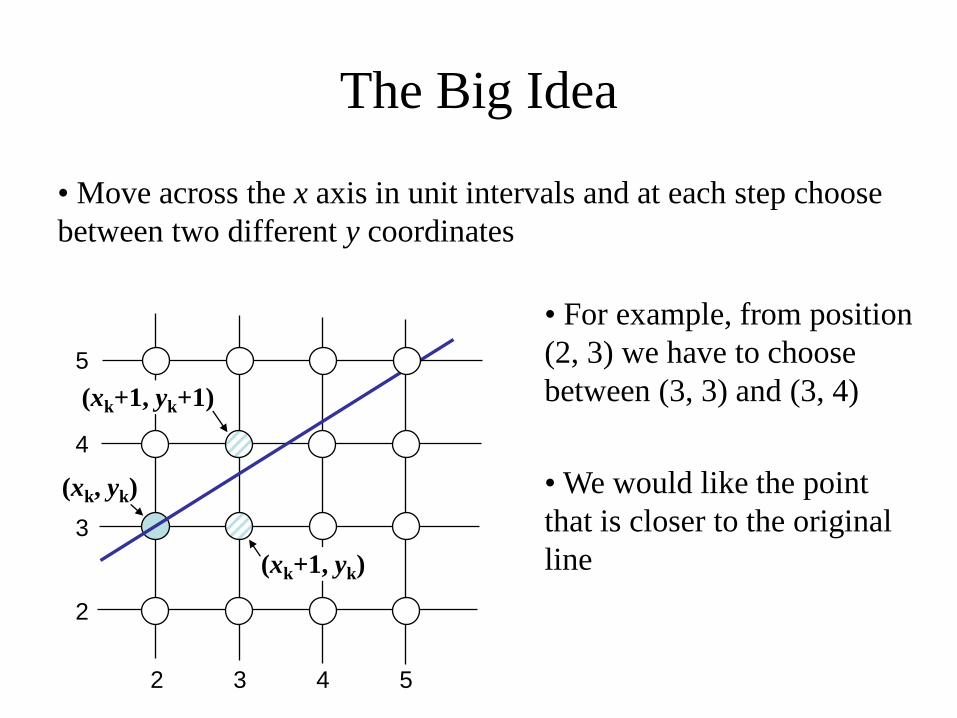
The Big Idea
• Move across the x axis in unit intervals and at each step choose
between two different y coordinates
2 3 4 5
2
4
3
5
• For example, from position
(2, 3) we have to choose
between (3, 3) and (3, 4)
• We would like the point
that is closer to the original
line
(xk, yk)
(xk+1, yk)
(xk+1, yk+1)
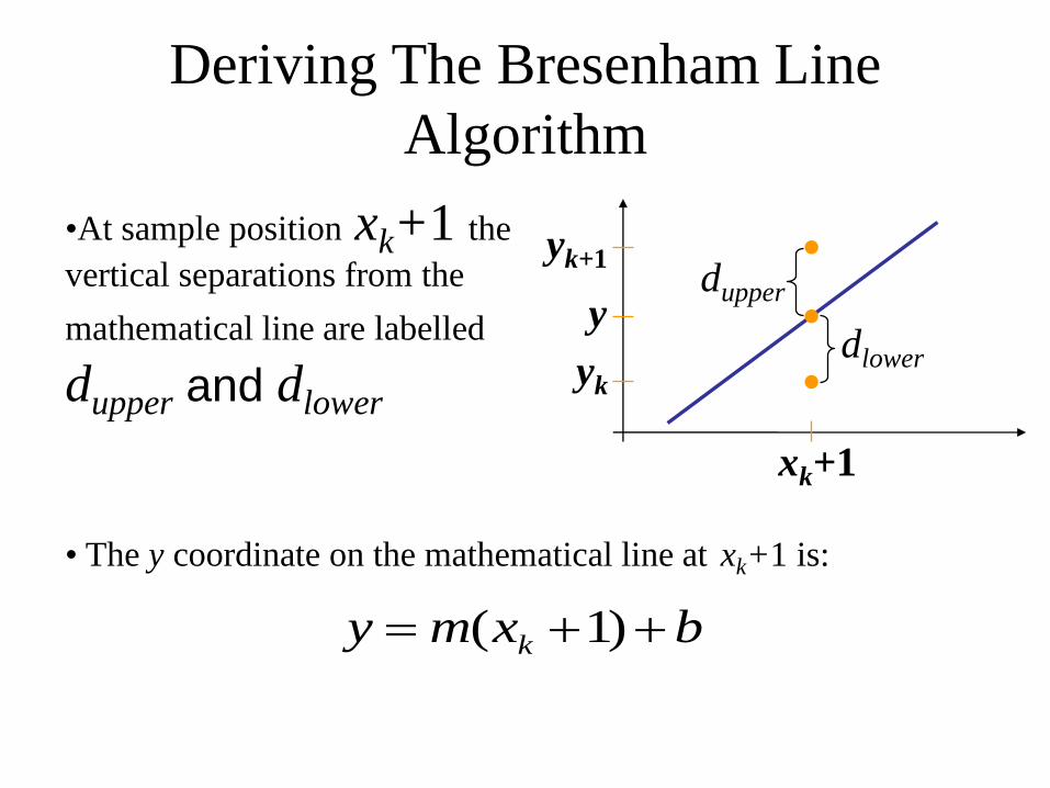
• The y coordinate on the mathematical line at xk+1 is:
Deriving The Bresenham Line
Algorithm
•At sample position xk+1 the
vertical separations from the
mathematical line are labelled
dupper and dlower
bxmy k )1(
y
yk
yk+1
xk+1
dlower
dupper
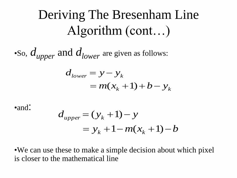
•So, dupper and dlower are given as follows:
•and:
•We can use these to make a simple decision about which pixel is closer to the mathematical line
Deriving The Bresenham Line
Algorithm (cont…)
klower yyd
kk ybxm )1(
yyd kupper )1(
bxmy kk )1(1
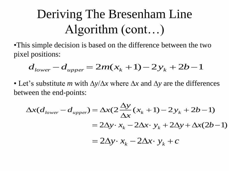
•This simple decision is based on the difference between the two
pixel positions:
• Let’s substitute m with ∆y/∆x where ∆x and ∆y are the differences
between the end-points:
Deriving The Bresenham Line
Algorithm (cont…)
122)1(2 byxmdd kkupperlower
)122)1(2()(
byx
x
yxddx kkupperlower
)12(222 bxyyxxy kk
cyxxy kk 22
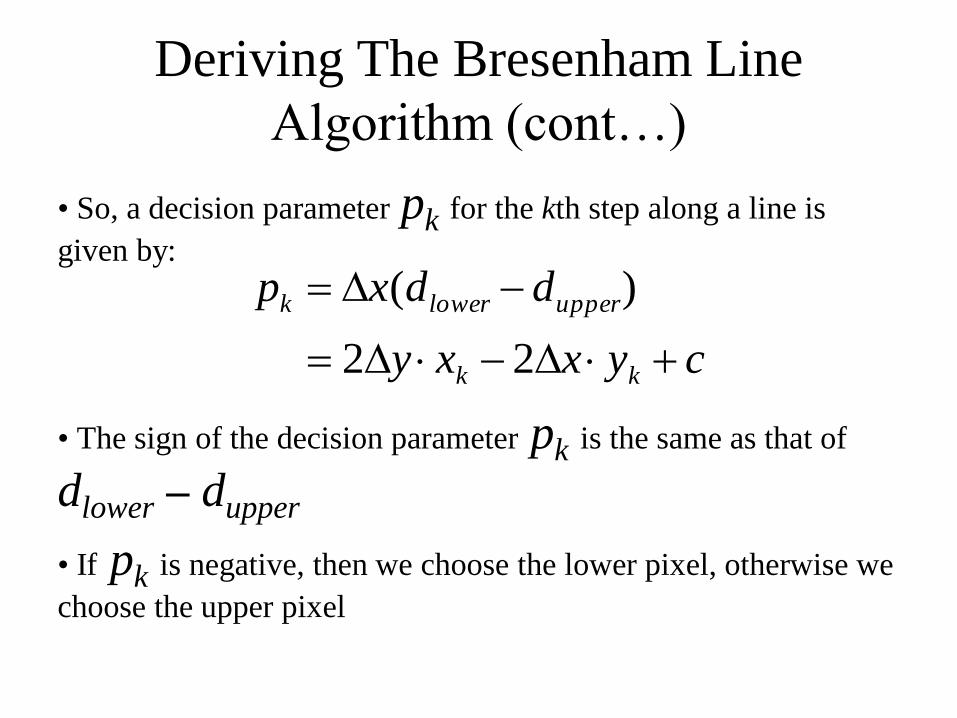
• So, a decision parameter pk for the kth step along a line is
given by:
• The sign of the decision parameter pk is the same as that of
dlower – dupper
• If pk is negative, then we choose the lower pixel, otherwise we
choose the upper pixel
Deriving The Bresenham Line
Algorithm (cont…)
cyxxy
ddxp
kk
upperlowerk
22
)(
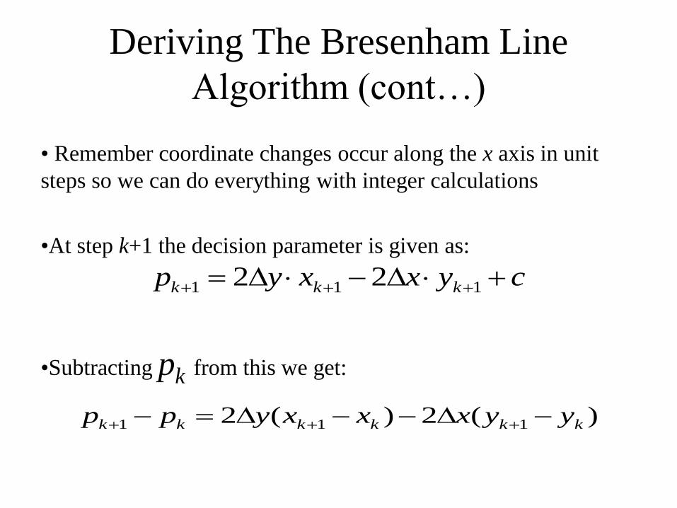
• Remember coordinate changes occur along the x axis in unit
steps so we can do everything with integer calculations
•At step k+1 the decision parameter is given as:
•Subtracting pk from this we get:
Deriving The Bresenham Line
Algorithm (cont…)
cyxxyp kkk 111 22
)(2)(2 111 kkkkkk yyxxxypp
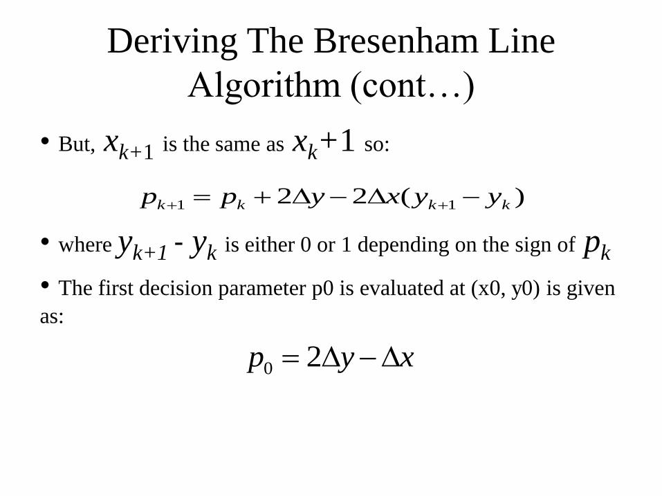
• But, xk+1 is the same as xk+1 so:
• where yk+1 - yk is either 0 or 1 depending on the sign of pk
• The first decision parameter p0 is evaluated at (x0, y0) is given
as:
Deriving The Bresenham Line
Algorithm (cont…)
)(22 11 kkkk yyxypp
xyp 20
The Bresenham Line Algorithm
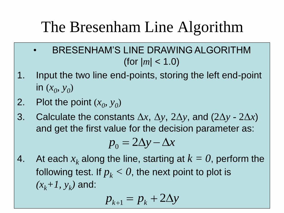
• BRESENHAM’S LINE DRAWING ALGORITHM
(for |m| < 1.0)
1. Input the two line end-points, storing the left end-point
in (x0, y0)
2. Plot the point (x0, y0)
3. Calculate the constants Δx, Δy, 2Δy, and (2Δy - 2Δx)
and get the first value for the decision parameter as:
4. At each xk along the line, starting at k = 0, perform the
following test. If pk < 0, the next point to plot is
(xk+1, yk) and:
xyp 20
ypp kk 21
The Bresenham Line Algorithm
(cont…)
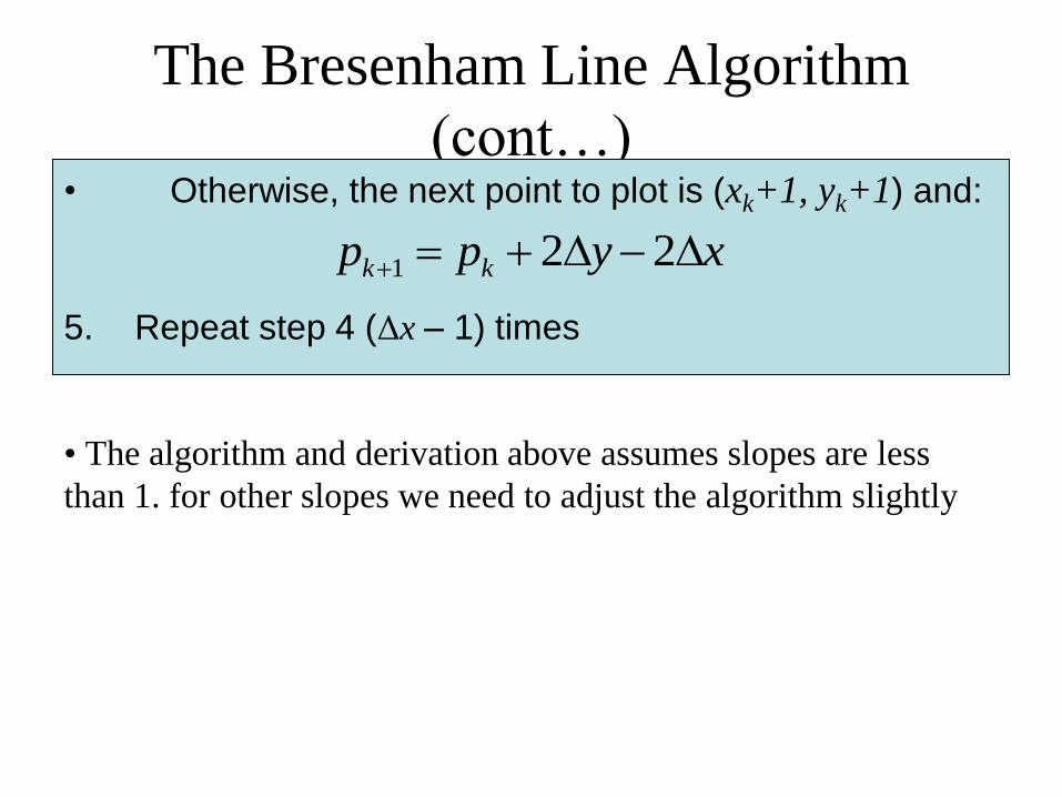
• The algorithm and derivation above assumes slopes are less
than 1. for other slopes we need to adjust the algorithm slightly
• Otherwise, the next point to plot is (xk+1, yk+1) and:
5. Repeat step 4 (Δx – 1) times
xypp kk 221
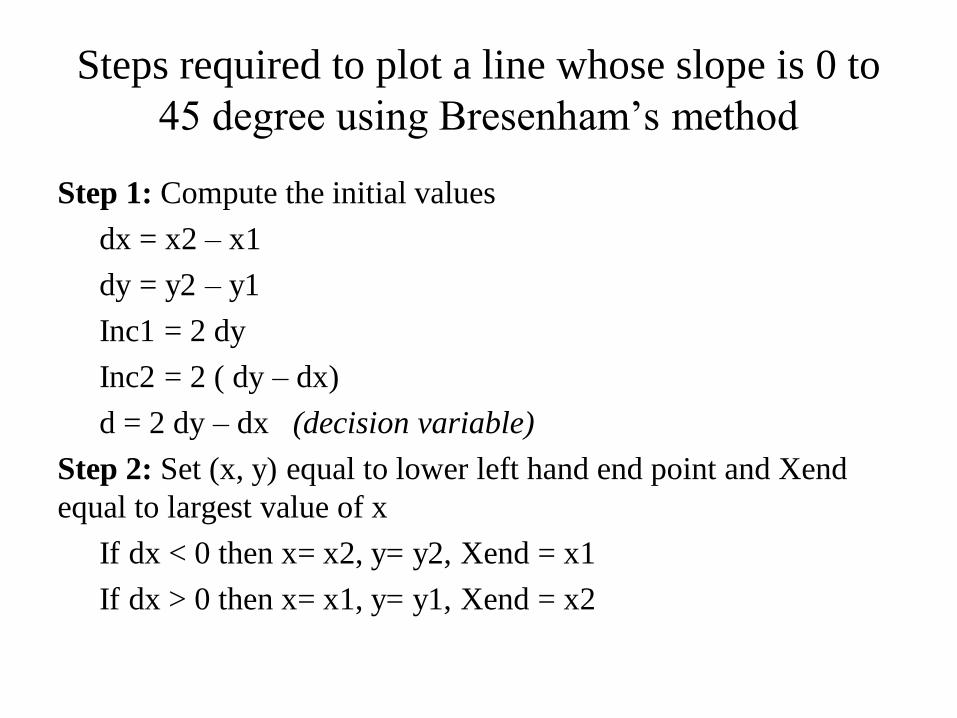
Steps required to plot a line whose slope is 0 to
45 degree using Bresenham’s method
Step 1: Compute the initial values
dx = x2 – x1
dy = y2 – y1
Inc1 = 2 dy
Inc2 = 2 ( dy – dx)
d = 2 dy – dx (decision variable)
Step 2: Set (x, y) equal to lower left hand end point and Xend
equal to largest value of x
If dx < 0 then x= x2, y= y2, Xend = x1
If dx > 0 then x= x1, y= y1, Xend = x2

Steps required to plot a line whose slope is 0 to
45 degree using Bresenham’s method (Cont..)
Step 3: Plot the point at the current (x, y) coordinates
Step 4: If x ≥ Xend stop
Step 5: Compute the location of next pixel
If d < 0 then d = d + Inc1
If d ≥ 0 then d = d + Inc2 and y = y + 1
Step 6: Increment x: x = x + 1
Step 7: Plot a line at the current (x, y) coordinates
Step 8: go to step 4
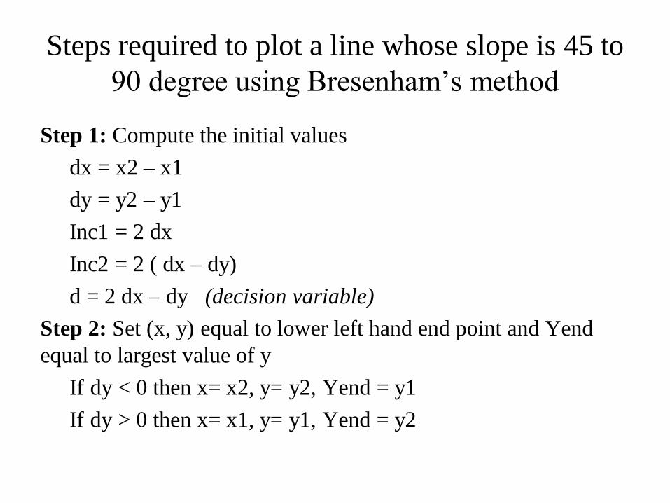
Steps required to plot a line whose slope is 45 to
90 degree using Bresenham’s method
Step 1: Compute the initial values
dx = x2 – x1
dy = y2 – y1
Inc1 = 2 dx
Inc2 = 2 ( dx – dy)
d = 2 dx – dy (decision variable)
Step 2: Set (x, y) equal to lower left hand end point and Yend
equal to largest value of y
If dy < 0 then x= x2, y= y2, Yend = y1
If dy > 0 then x= x1, y= y1, Yend = y2
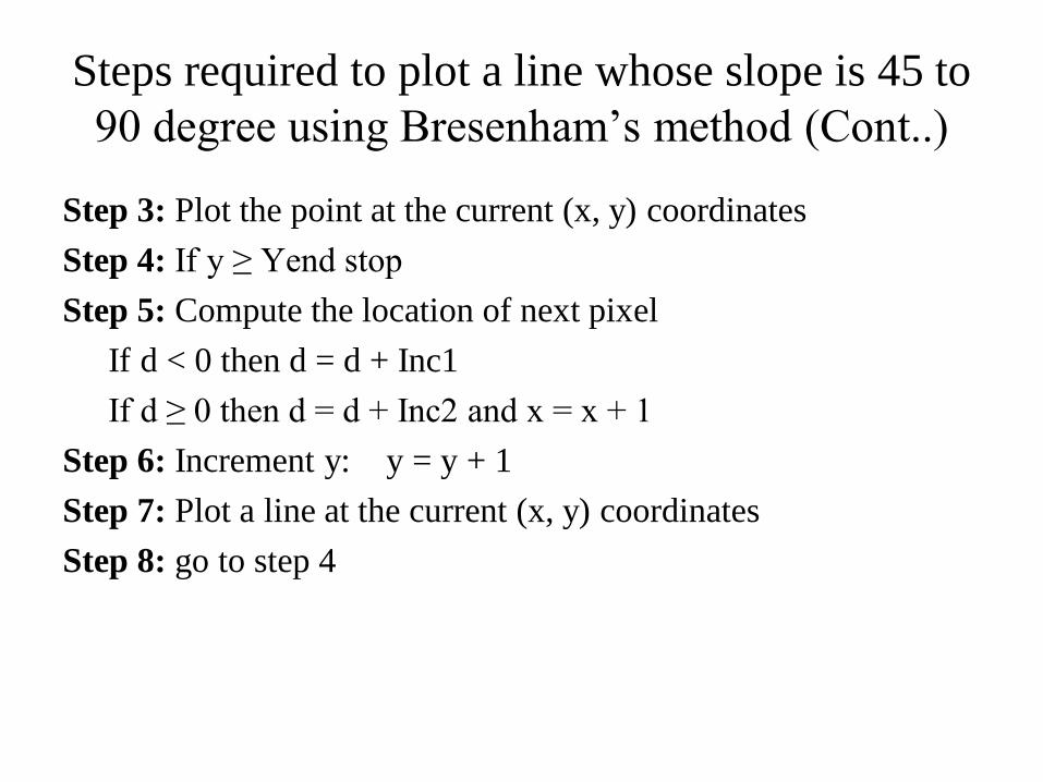
Steps required to plot a line whose slope is 45 to
90 degree using Bresenham’s method (Cont..)
Step 3: Plot the point at the current (x, y) coordinates
Step 4: If y ≥ Yend stop
Step 5: Compute the location of next pixel
If d < 0 then d = d + Inc1
If d ≥ 0 then d = d + Inc2 and x = x + 1
Step 6: Increment y: y = y + 1
Step 7: Plot a line at the current (x, y) coordinates
Step 8: go to step 4
Bresenham Line Algorithm Summary
• The Bresenham line algorithm has the following advantages:
– A fast incremental algorithm
– Uses only integer calculations
Bresenham is not the end
•J.G. Rokne, Brian WyVill, Xiolin Wu, Fast Line Scan
Conversion, ACM Transaction on Graphics, 9 (4), pp 376-388,
1990.
– Claims to be 4-times faster than Bresenham’s

Circle Scan Conversion
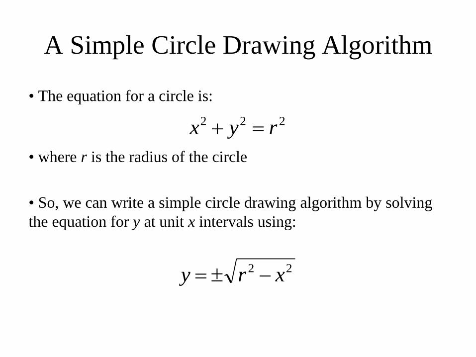
A Simple Circle Drawing Algorithm
• The equation for a circle is:
• where r is the radius of the circle
• So, we can write a simple circle drawing algorithm by solving
the equation for y at unit x intervals using:
222 ryx
22 xry
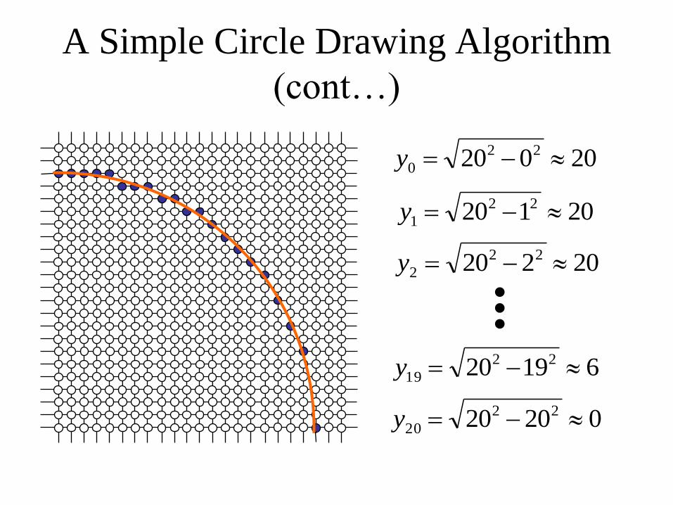
A Simple Circle Drawing Algorithm
(cont…)
20020 22
0 y
20120 22
1 y
20220 22
2 y
61920 22
19 y
02020 22
20 y
A Simple Circle Drawing Algorithm
(cont…) • However, unsurprisingly this is not a brilliant solution!
• Firstly, the resulting circle has large gaps where the slope approaches the vertical
• Secondly, the calculations are not very efficient
– The square (multiply) operations
– The square root operation – try really hard to avoid these!
• We need a more efficient, more accurate solution
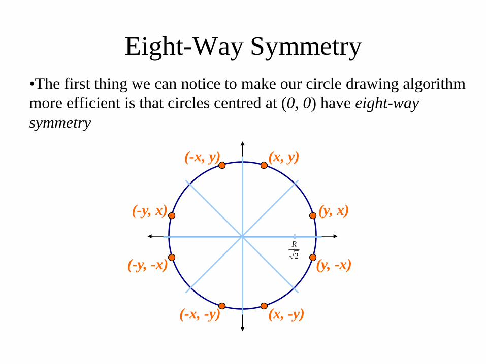
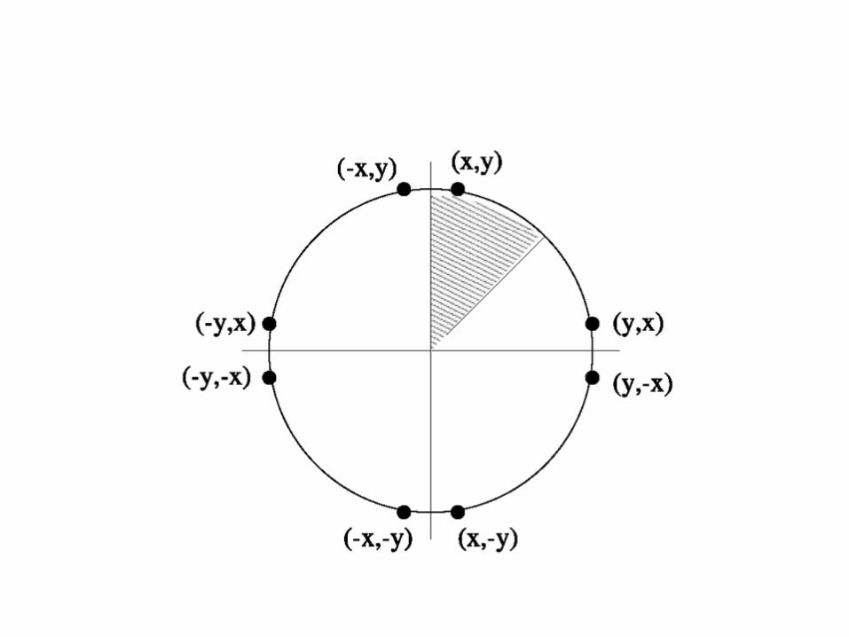
Eight-Way Symmetry
•The first thing we can notice to make our circle drawing algorithm
more efficient is that circles centred at (0, 0) have eight-way
symmetry
(x, y)
(y, x)
(y, -x)
(x, -y) (-x, -y)
(-y, -x)
(-y, x)
(-x, y)
2
R
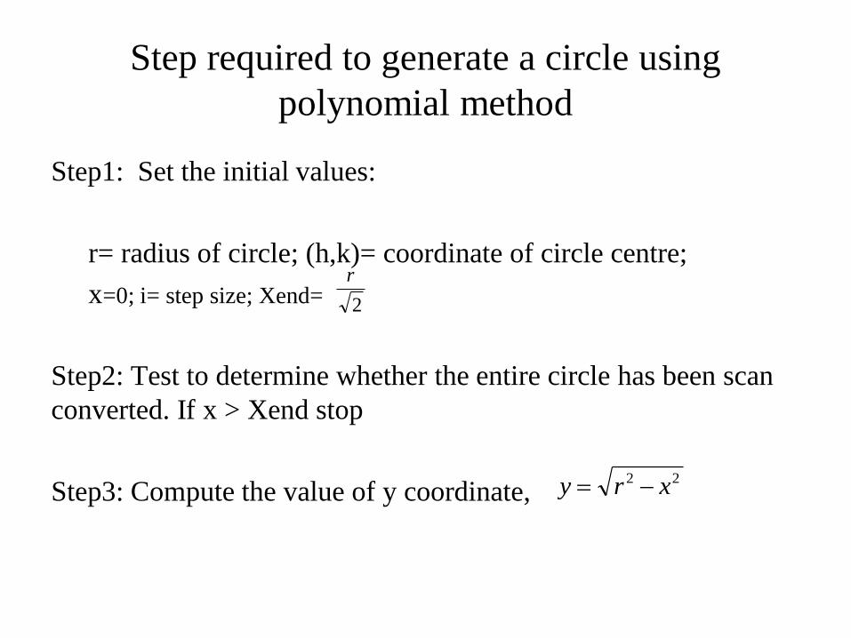
Step required to generate a circle using
polynomial method
Step1: Set the initial values:
r= radius of circle; (h,k)= coordinate of circle centre;
x=0; i= step size; Xend=
Step2: Test to determine whether the entire circle has been scan
converted. If x > Xend stop
Step3: Compute the value of y coordinate,
2
r
22 xry
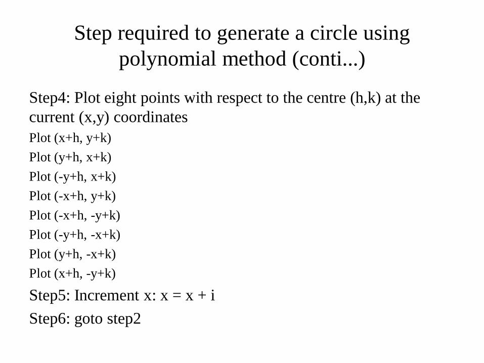
Step required to generate a circle using
polynomial method (conti...)
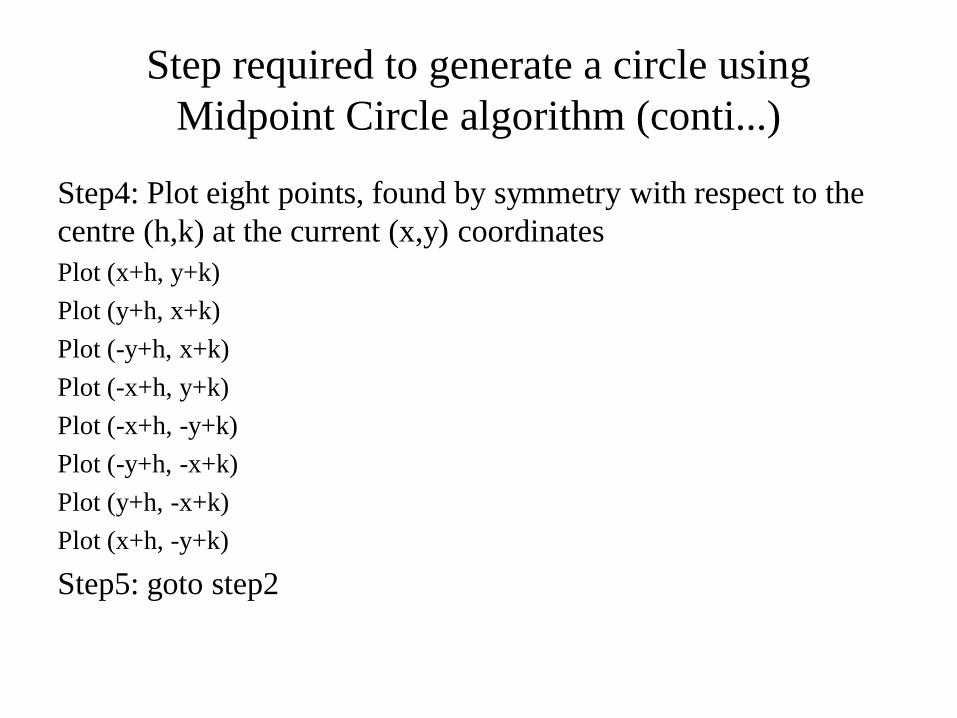
Step4: Plot eight points with respect to the centre (h,k) at the
current (x,y) coordinates
Plot (x+h, y+k)
Plot (y+h, x+k)
Plot (-y+h, x+k)
Plot (-x+h, y+k)
Plot (-x+h, -y+k)
Plot (-y+h, -x+k)
Plot (y+h, -x+k)
Plot (x+h, -y+k)
Step5: Increment x: x = x + i
Step6: goto step2
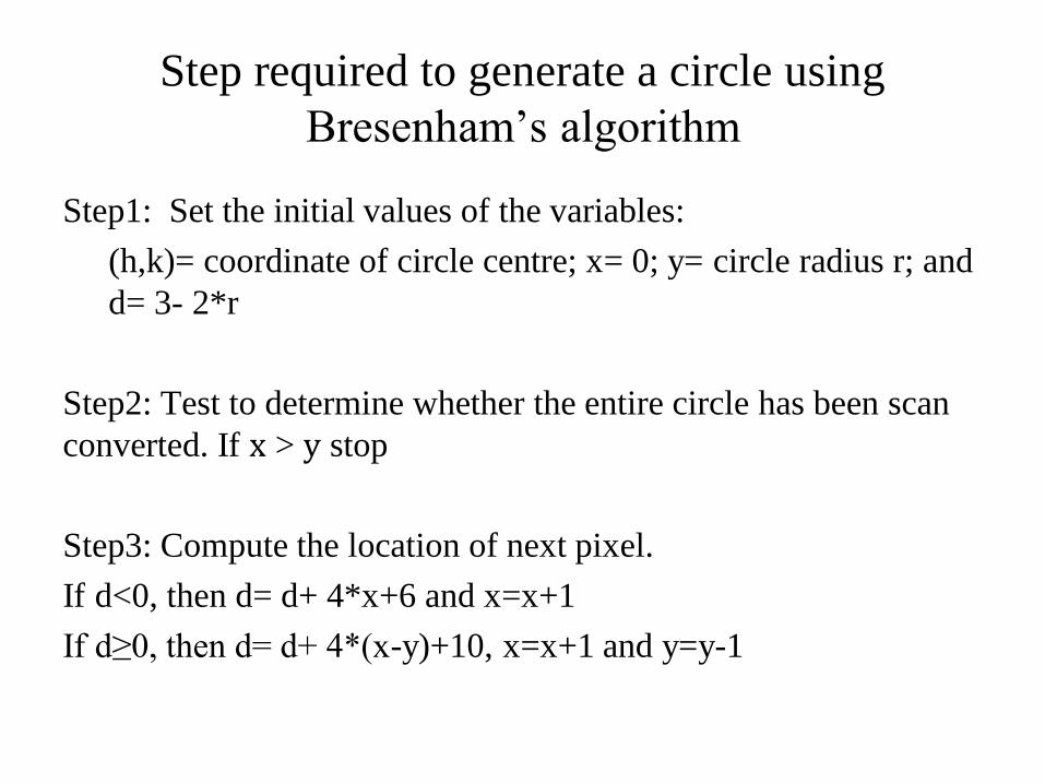
Step required to generate a circle using
Bresenham’s algorithm
Step1: Set the initial values of the variables:
(h,k)= coordinate of circle centre; x= 0; y= circle radius r; and
d= 3- 2*r
Step2: Test to determine whether the entire circle has been scan
converted. If x > y stop
Step3: Compute the location of next pixel.
If d<0, then d= d+ 4*x+6 and x=x+1
If d≥0, then d= d+ 4*(x-y)+10, x=x+1 and y=y-1
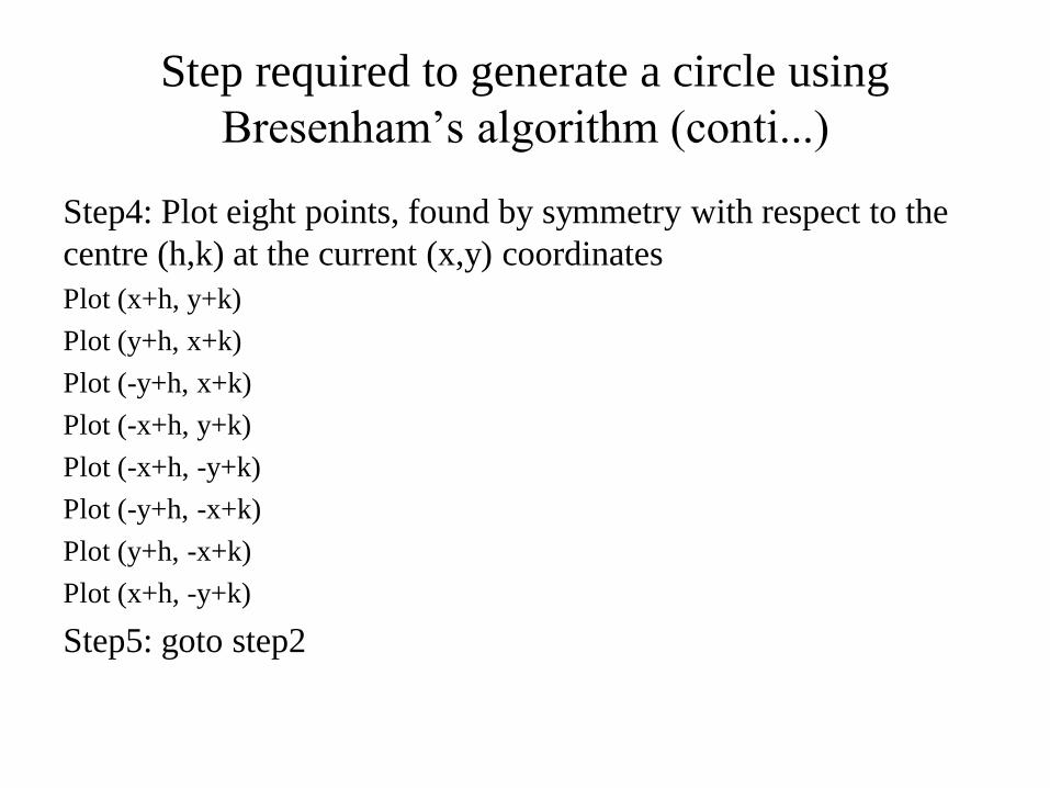
Step required to generate a circle using
Bresenham’s algorithm (conti...)
Step4: Plot eight points, found by symmetry with respect to the
centre (h,k) at the current (x,y) coordinates
Plot (x+h, y+k)
Plot (y+h, x+k)
Plot (-y+h, x+k)
Plot (-x+h, y+k)
Plot (-x+h, -y+k)
Plot (-y+h, -x+k)
Plot (y+h, -x+k)
Plot (x+h, -y+k)
Step5: goto step2
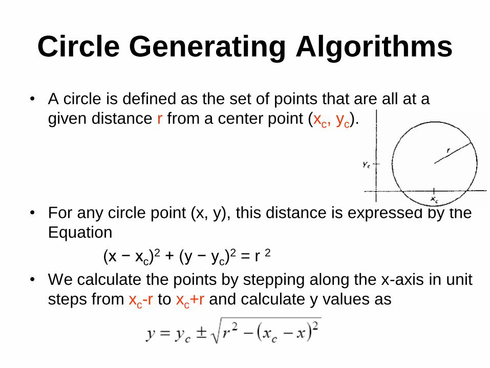
Circle Generating Algorithms
• A circle is defined as the set of points that are all at a
given distance r from a center point (xc, yc).
• For any circle point (x, y), this distance is expressed by the
Equation
(x − xc)2 + (y − yc)
2 = r 2
• We calculate the points by stepping along the x-axis in unit
steps from xc-r to xc+r and calculate y values as
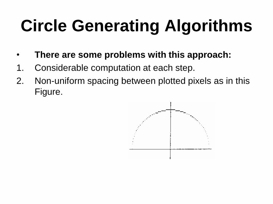
Circle Generating Algorithms
• There are some problems with this approach:
1. Considerable computation at each step.
2. Non-uniform spacing between plotted pixels as in this
Figure.
Circle Generating Algorithms
• Problem 2 can be removed using the polar
form:
x = xc + r cos θ
y = yc + r sin θ
• using a fixed angular step size, a circle is
plotted with equally spaced points along
the circumference.
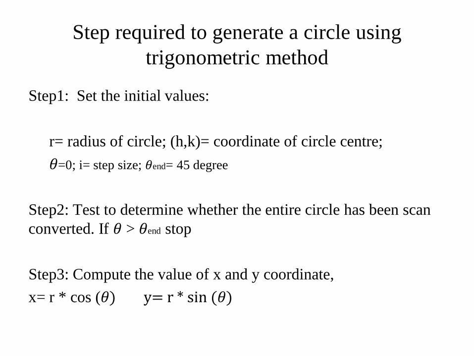
Step required to generate a circle using
trigonometric method
Step1: Set the initial values:
r= radius of circle; (h,k)= coordinate of circle centre;
𝜃=0; i= step size; 𝜃end= 45 degree
Step2: Test to determine whether the entire circle has been scan
converted. If 𝜃 > 𝜃end stop
Step3: Compute the value of x and y coordinate,
x= r * cos (𝜃) y= r * sin (𝜃)
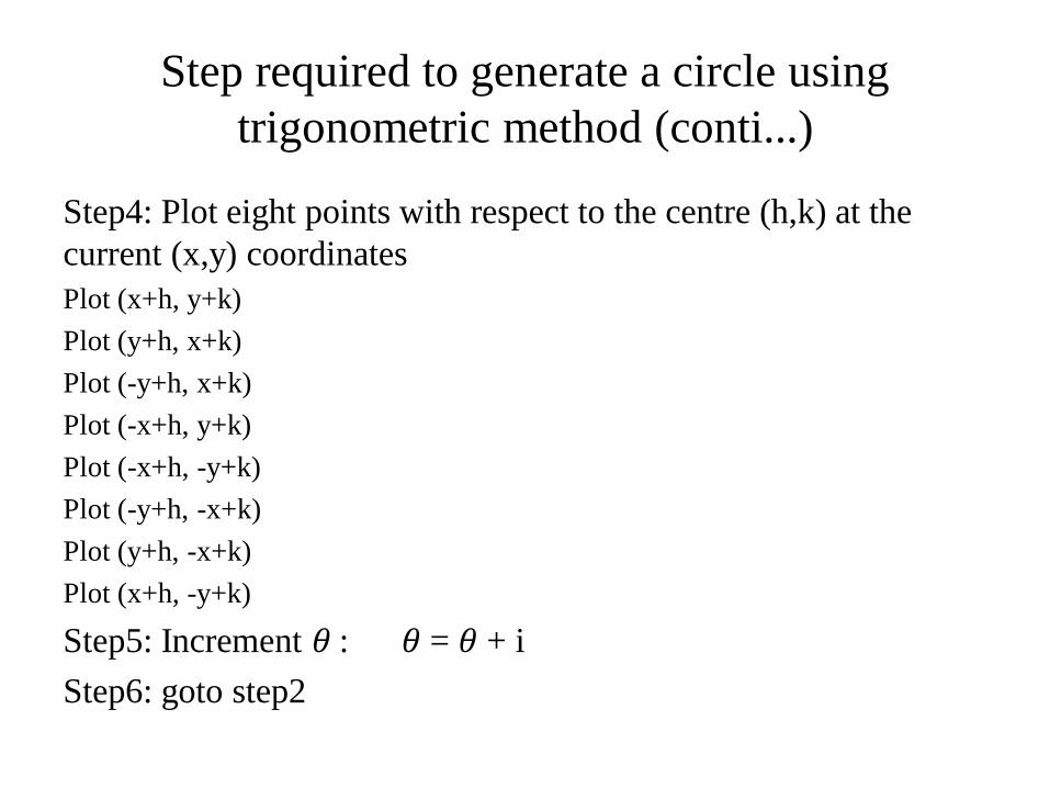
Step required to generate a circle using
trigonometric method (conti...)
Step4: Plot eight points with respect to the centre (h,k) at the
current (x,y) coordinates
Plot (x+h, y+k)
Plot (y+h, x+k)
Plot (-y+h, x+k)
Plot (-x+h, y+k)
Plot (-x+h, -y+k)
Plot (-y+h, -x+k)
Plot (y+h, -x+k)
Plot (x+h, -y+k)
Step5: Increment 𝜃 : 𝜃 = 𝜃 + i
Step6: goto step2
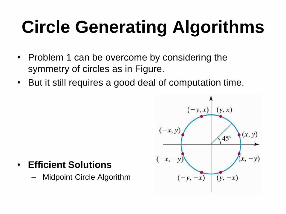
Circle Generating Algorithms
• Problem 1 can be overcome by considering the
symmetry of circles as in Figure.
• But it still requires a good deal of computation time.
• Efficient Solutions
– Midpoint Circle Algorithm
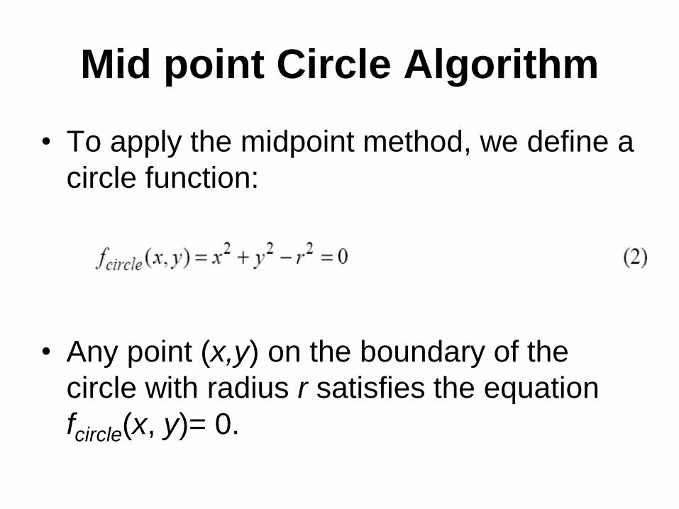
Mid point Circle Algorithm
• To apply the midpoint method, we define a
circle function:
• Any point (x,y) on the boundary of the
circle with radius r satisfies the equation
fcircle(x, y)= 0.
Mid point Circle Algorithm
• If the points is in the interior of the circle,
the circle function is negative.
• If the point is outside the circle, the circle
function is positive.
• To summarize, the relative position of any
point (x,y) can be determined by checking
the sign of the circle function:
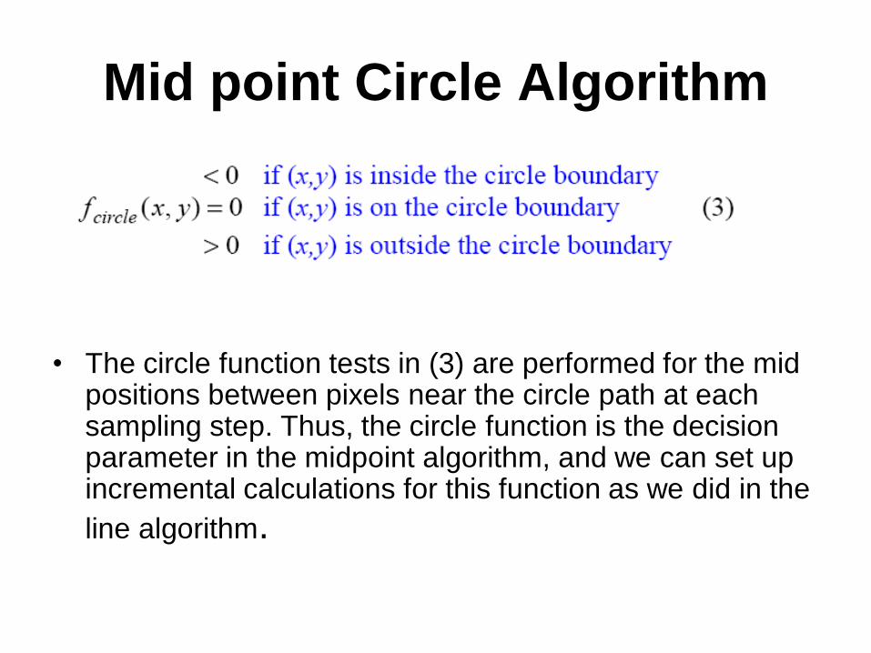
Mid point Circle Algorithm
• The circle function tests in (3) are performed for the mid positions between pixels near the circle path at each sampling step. Thus, the circle function is the decision parameter in the midpoint algorithm, and we can set up incremental calculations for this function as we did in the
line algorithm.
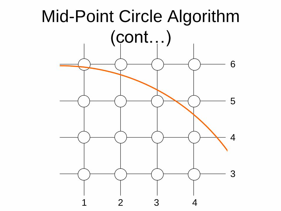
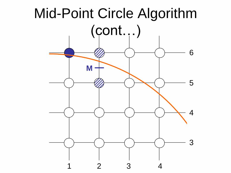
Mid point Circle Algorithm
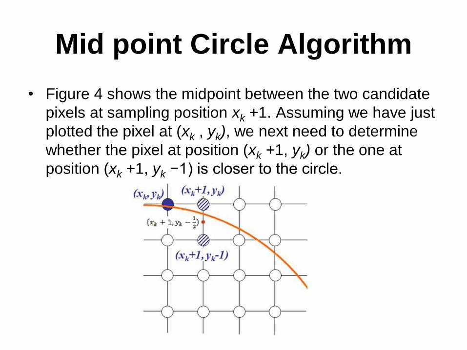
• Figure 4 shows the midpoint between the two candidate
pixels at sampling position xk +1. Assuming we have just
plotted the pixel at (xk , yk), we next need to determine
whether the pixel at position (xk +1, yk) or the one at
position (xk +1, yk −1) is closer to the circle.
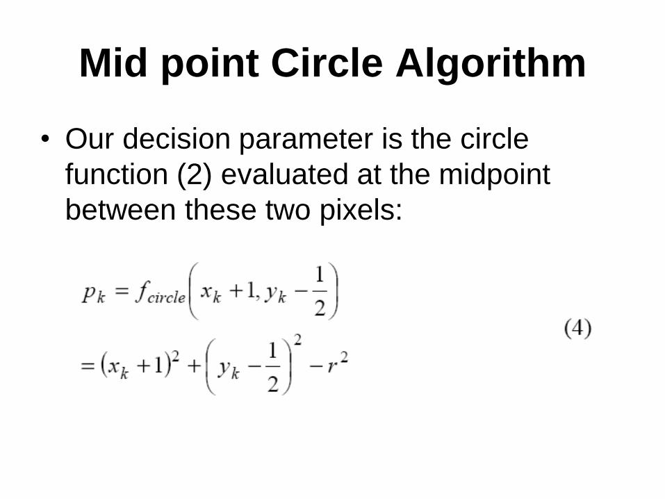
Mid point Circle Algorithm
• Our decision parameter is the circle
function (2) evaluated at the midpoint
between these two pixels:
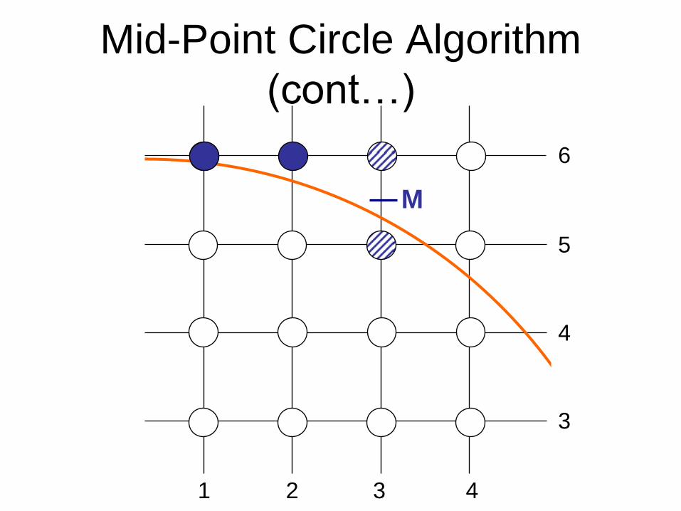
Mid point Circle Algorithm
• If pk < 0, this midpoint is inside the circle
and the pixel on scan line yk is closer to
the circle boundary.
• Otherwise, the midpoint is outside or on
the circle boundary, and we select the
pixel on scan line yk −1.
• Successive decision parameters are
obtained using incremental calculations.
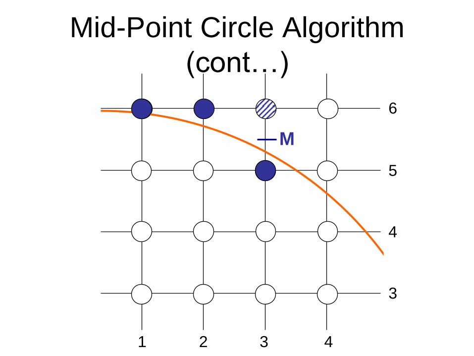
Mid point Circle Algorithm
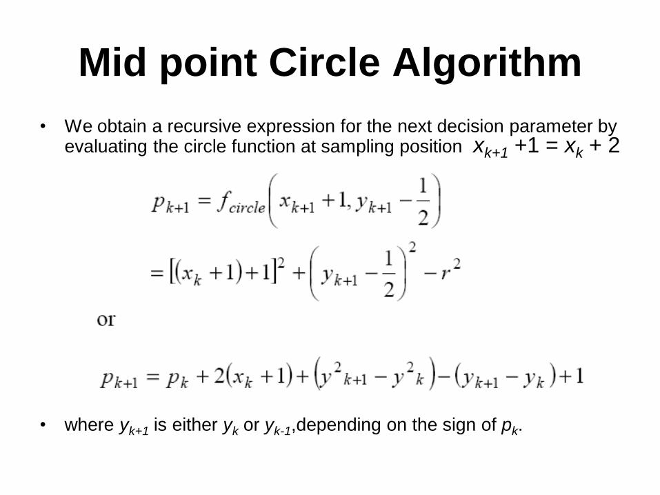
• We obtain a recursive expression for the next decision parameter by evaluating the circle function at sampling position xk+1 +1 = xk + 2
• where yk+1 is either yk or yk-1,depending on the sign of pk.
Mid point Circle Algorithm
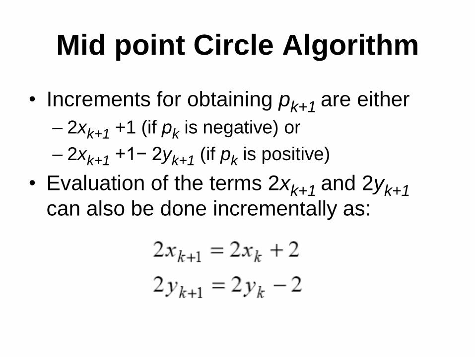
• Increments for obtaining pk+1 are either
– 2xk+1 +1 (if pk is negative) or
– 2xk+1 +1− 2yk+1 (if pk is positive)
• Evaluation of the terms 2xk+1 and 2yk+1
can also be done incrementally as:
Mid point Circle Algorithm
• At the start position (0, r), these two terms
(2x, 2y) have the values 0 and 2r,
respectively.
• Each successive value is obtained by
adding 2 to the previous value of 2x and
subtracting 2 from the previous value of
2y.
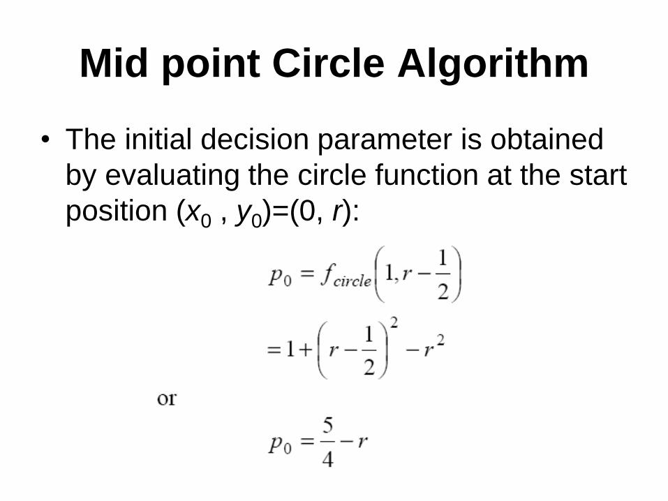
Mid point Circle Algorithm
• The initial decision parameter is obtained
by evaluating the circle function at the start
position (x0 , y0)=(0, r):
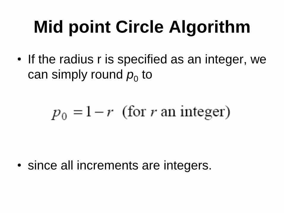
Mid point Circle Algorithm
• If the radius r is specified as an integer, we
can simply round p0 to
• since all increments are integers.

Summary of the Algorithm
• As in Bresenham’s line algorithm, the
midpoint method calculates pixel positions
along the circumference of a circle using
integer additions and subtractions,
assuming that the circle parameters are
specified in screen coordinates. We can
summarize the steps in the midpoint circle
algorithm as follows.
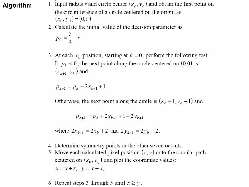
Algorithm
Mid-Point Circle Algorithm
(cont…)
6
2 3 4 1
5
4
3
Mid-Point Circle Algorithm
(cont…)
M
6
2 3 4 1
5
4
3
Mid-Point Circle Algorithm
(cont…)
M
6
2 3 4 1
5
4
3
Mid-Point Circle Algorithm
(cont…)
M
6
2 3 4 1
5
4
3
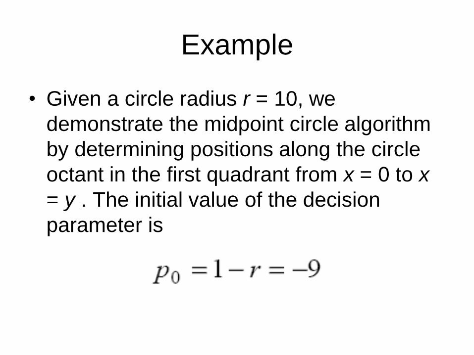
Example
• Given a circle radius r = 10, we
demonstrate the midpoint circle algorithm
by determining positions along the circle
octant in the first quadrant from x = 0 to x
= y . The initial value of the decision
parameter is
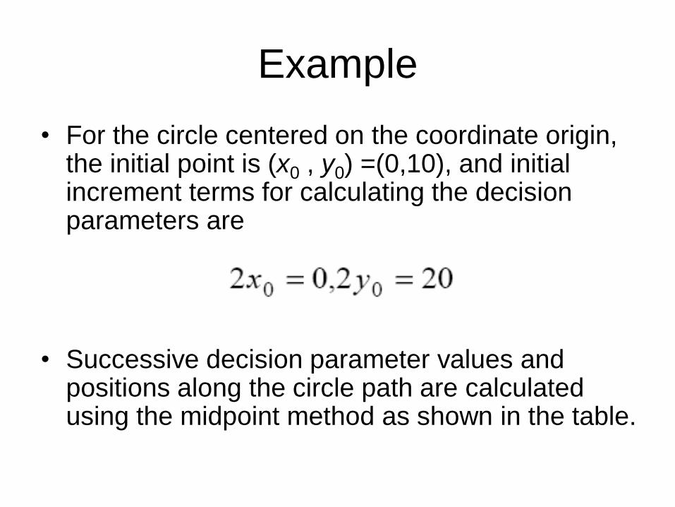
Example
• For the circle centered on the coordinate origin, the initial point is (x0 , y0) =(0,10), and initial increment terms for calculating the decision parameters are
• Successive decision parameter values and positions along the circle path are calculated using the midpoint method as shown in the table.
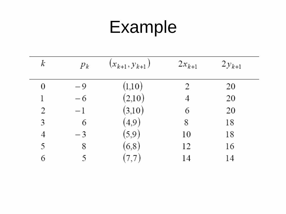
Example
Example
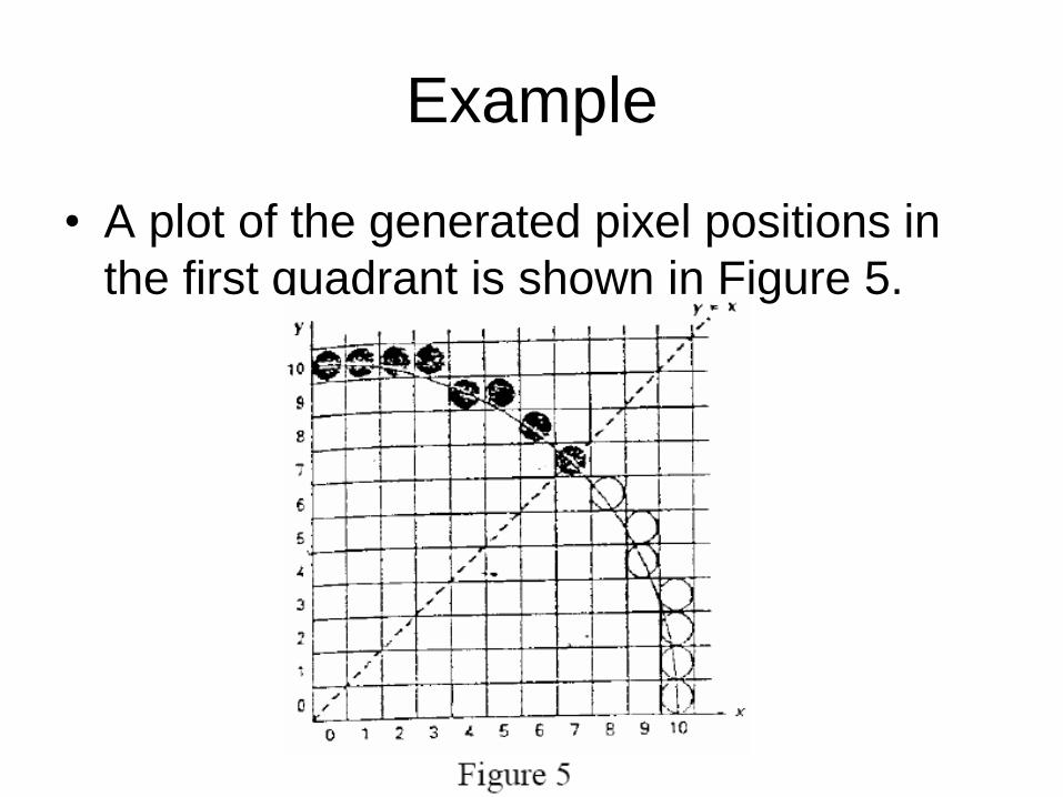
• A plot of the generated pixel positions in
the first quadrant is shown in Figure 5.
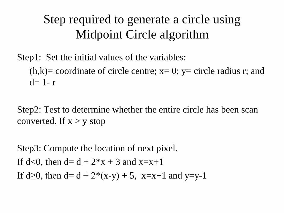
Step required to generate a circle using
Midpoint Circle algorithm
Step1: Set the initial values of the variables:
(h,k)= coordinate of circle centre; x= 0; y= circle radius r; and
d= 1- r
Step2: Test to determine whether the entire circle has been scan
converted. If x > y stop
Step3: Compute the location of next pixel.
If d<0, then d= d + 2*x + 3 and x=x+1
If d≥0, then d= d + 2*(x-y) + 5, x=x+1 and y=y-1
Step required to generate a circle using
Midpoint Circle algorithm (conti...)
Step4: Plot eight points, found by symmetry with respect to the
centre (h,k) at the current (x,y) coordinates
Plot (x+h, y+k)
Plot (y+h, x+k)
Plot (-y+h, x+k)
Plot (-x+h, y+k)
Plot (-x+h, -y+k)
Plot (-y+h, -x+k)
Plot (y+h, -x+k)
Plot (x+h, -y+k)
Step5: goto step2
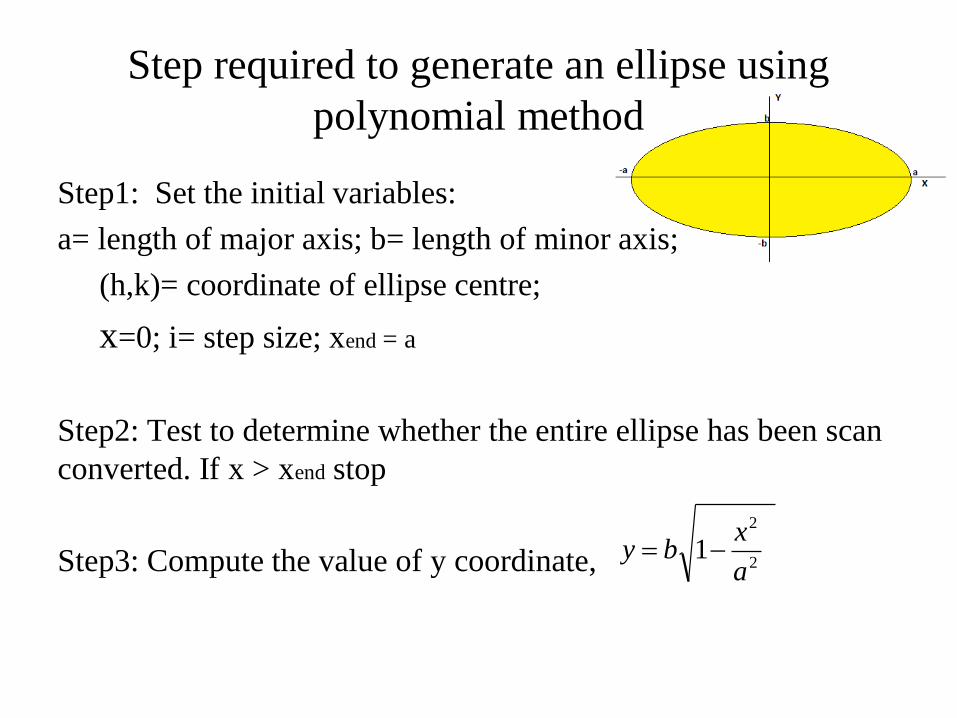
Step required to generate an ellipse using
polynomial method
Step1: Set the initial variables:
a= length of major axis; b= length of minor axis;
(h,k)= coordinate of ellipse centre;
x=0; i= step size; xend = a
Step2: Test to determine whether the entire ellipse has been scan
converted. If x > xend stop
Step3: Compute the value of y coordinate,
2
2
1a
xby
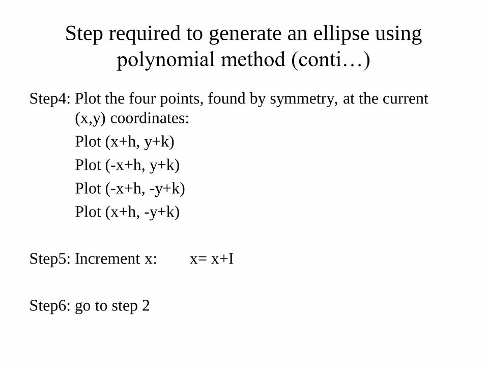
Step required to generate an ellipse using
polynomial method (conti…)
Step4: Plot the four points, found by symmetry, at the current
(x,y) coordinates:
Plot (x+h, y+k)
Plot (-x+h, y+k)
Plot (-x+h, -y+k)
Plot (x+h, -y+k)
Step5: Increment x: x= x+I
Step6: go to step 2

Fill Area Algorithms
Polygon Fill Algorithm
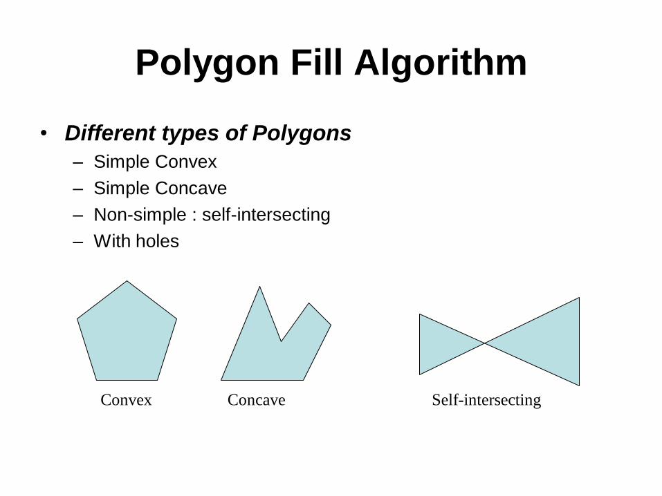
• Different types of Polygons
– Simple Convex
– Simple Concave
– Non-simple : self-intersecting
– With holes
Convex Concave Self-intersecting
Polygon Fill Algorithm
• A scan-line fill algorithm of a region is performed as follows: 1. Determining the intersection positions of the
boundaries of the fill region with the screen scan lines.
2. Then the fill colors are applied to each section of a scan line that lies within the interior of the fill region.
• The simplest area to fill is a polygon, because each scan-line intersection point with a polygon boundary is obtained by solving a pair of simultaneous linear equations, where the equation for the scan line is simply y = constant.
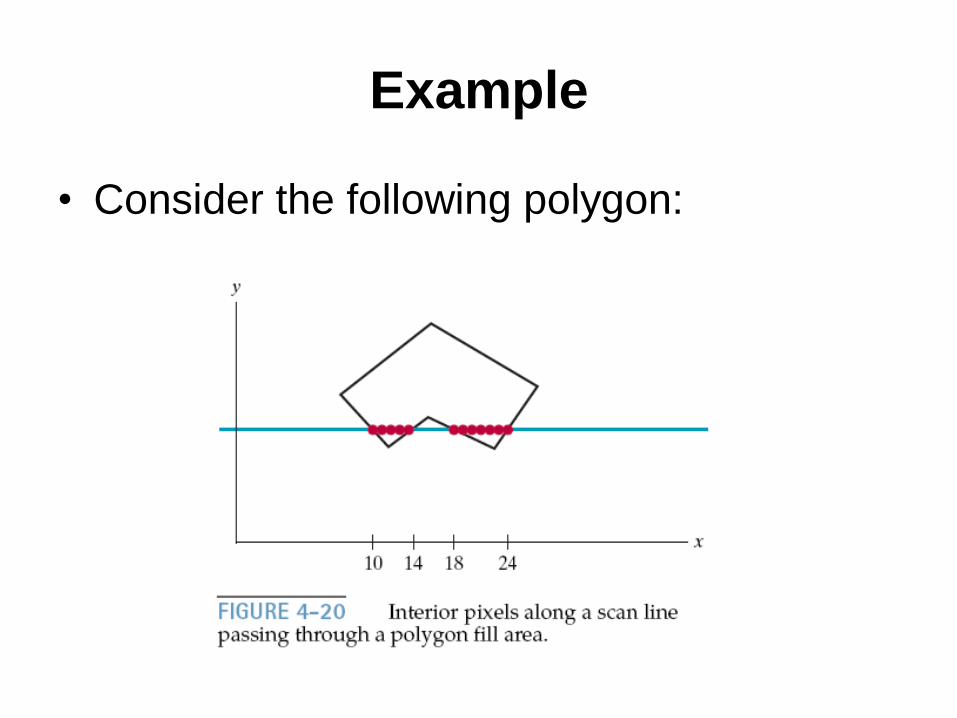
Example
• Consider the following polygon:
Example
• For each scan line that crosses the polygon, the
edge intersections are sorted from left to right,
and then the pixel positions between, and
including, each intersection pair are set to the
specified fill color.
• In the previous Figure, the four pixel intersection
positions with the polygon boundaries define two
stretches of interior pixels.
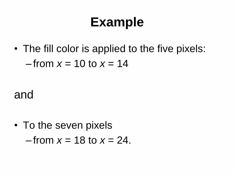
Example
• The fill color is applied to the five pixels:
– from x = 10 to x = 14
and
• To the seven pixels
– from x = 18 to x = 24.
Polygon Fill Algorithm
• However, the scan-line fill algorithm for a
polygon is not quite as simple
• Whenever a scan line passes through a
vertex, it intersects two polygon edges at
that point.
• In some cases, this can result in an odd
number of boundary intersections for a
scan line.
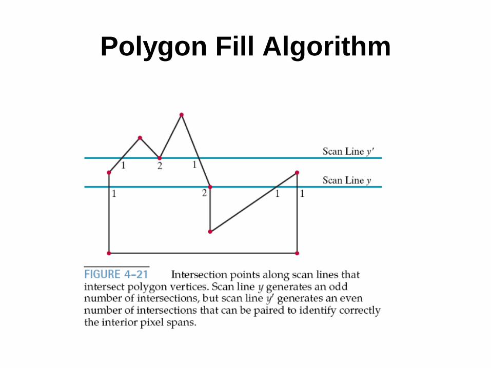
Polygon Fill Algorithm
• Consider the next Figure.
• It shows two scan lines that cross a polygon fill area and intersect a vertex.
• Scan line y’ intersects an even number of edges, and the two pairs of intersection points along this scan line correctly identify the interior pixel spans.
• But scan line y intersects five polygon edges.
Polygon Fill Algorithm
Polygon Fill Algorithm
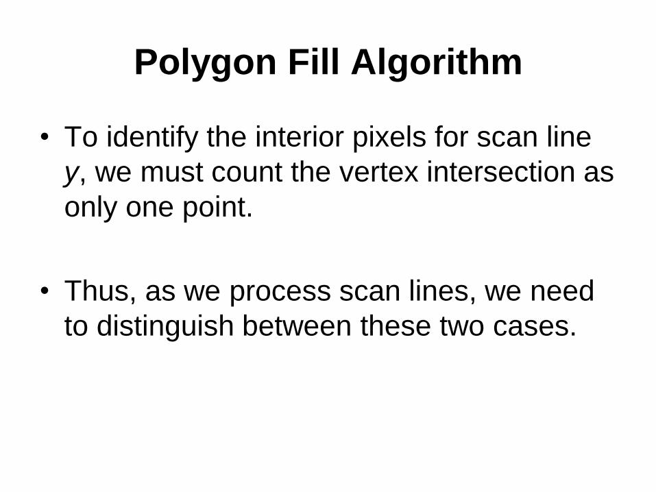
• To identify the interior pixels for scan line
y, we must count the vertex intersection as
only one point.
• Thus, as we process scan lines, we need
to distinguish between these two cases.
Polygon Fill Algorithm
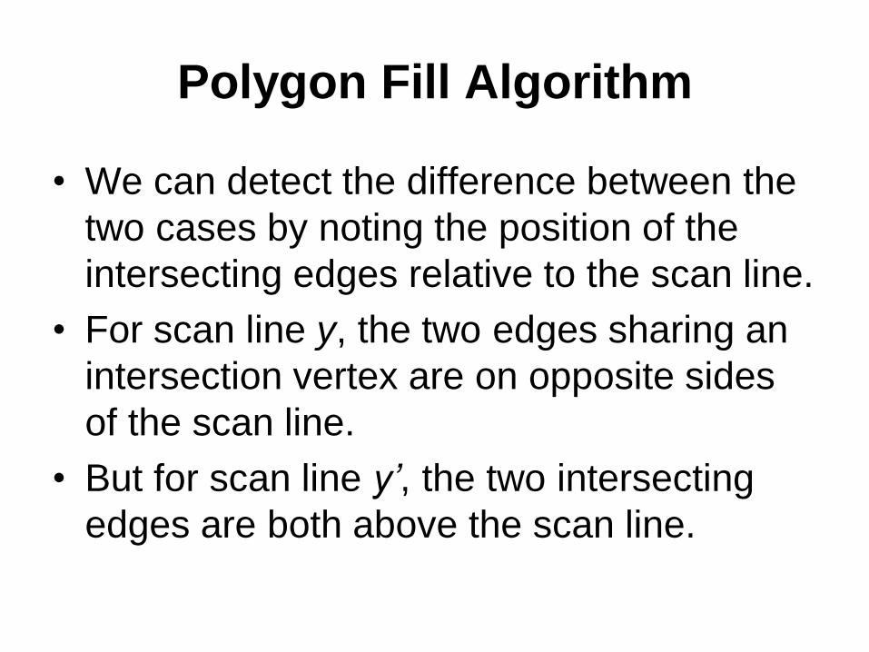
• We can detect the difference between the
two cases by noting the position of the
intersecting edges relative to the scan line.
• For scan line y, the two edges sharing an
intersection vertex are on opposite sides
of the scan line.
• But for scan line y’, the two intersecting
edges are both above the scan line.
Polygon Fill Algorithm
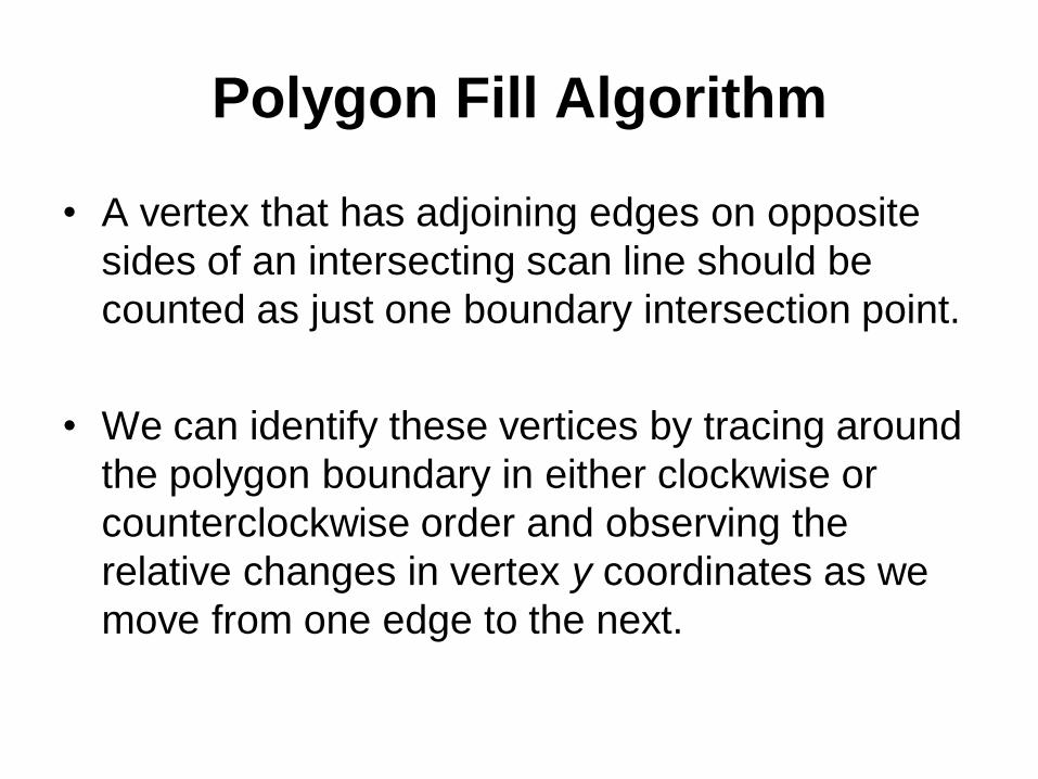
• A vertex that has adjoining edges on opposite
sides of an intersecting scan line should be
counted as just one boundary intersection point.
• We can identify these vertices by tracing around
the polygon boundary in either clockwise or
counterclockwise order and observing the
relative changes in vertex y coordinates as we
move from one edge to the next.
Polygon Fill Algorithm
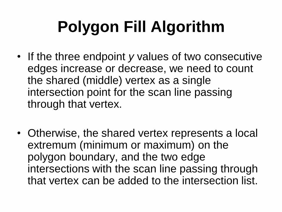
• If the three endpoint y values of two consecutive edges increase or decrease, we need to count the shared (middle) vertex as a single intersection point for the scan line passing through that vertex.
• Otherwise, the shared vertex represents a local extremum (minimum or maximum) on the polygon boundary, and the two edge intersections with the scan line passing through that vertex can be added to the intersection list.
Area Fill Algorithm
• An alternative approach for filling an area is to
start at a point inside the area and “paint” the
interior, point by point, out to the boundary.
• This is a particularly useful technique for filling
areas with irregular borders, such as a design
created with a paint program.
• The algorithm makes the following assumptions
– one interior pixel is known, and
– pixels in boundary are known.
Area Fill Algorithm
• If the boundary of some region is specified
in a single color, we can fill the interior of
this region, pixel by pixel, until the
boundary color is encountered.
• This method, called the boundary-fill
algorithm, is employed in interactive
painting packages, where interior points
are easily selected.
Example
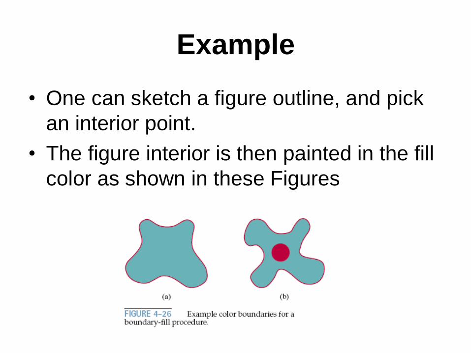
• One can sketch a figure outline, and pick
an interior point.
• The figure interior is then painted in the fill
color as shown in these Figures
Area Fill Algorithm
• Basically, a boundary-fill algorithm starts
from an interior point (x, y) and sets the
neighboring points to the desired color.
• This procedure continues until all pixels
are processed up to the designated
boundary for the area.
Area Fill Algorithm
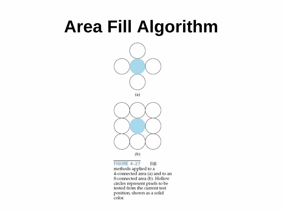
• There are two methods for processing
neighboring pixels from a current point.
1. Four neighboring points.
– These are the pixel positions that are right,
left, above, and below the current pixel.
– Areas filled by this method are called 4-
connected.
Area Fill Algorithm
2. Eight neighboring points.
– This method is used to fill more complex
figures.
– Here the set of neighboring points to be set
includes the four diagonal pixels, in addition to
the four points in the first method.
– Fill methods using this approach are called 8-
connected.
Area Fill Algorithm
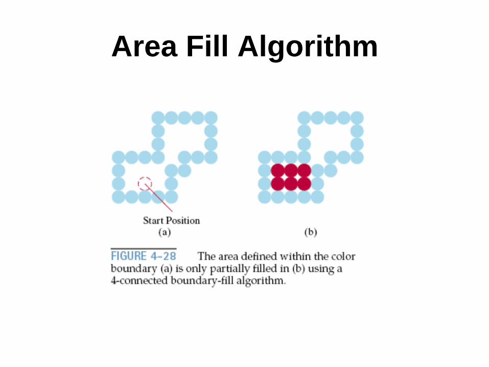
Area Fill Algorithm
• Consider the Figure in the next slide.
• An 8-connected boundary-fill algorithm
would correctly fill the interior of the area
defined in the Figure.
• But a 4-connected boundary-fill algorithm
would only fill part of that region.
Area Fill Algorithm
Area Fill Algorithm
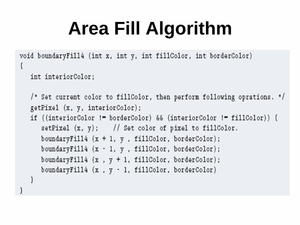
• The following procedure illustrates a recursive
method for painting a 4-connected area with a
solid color, specified in parameter fillColor, up
to a boundary color specified with parameter
borderColor.
• We can extend this procedure to fill an 8-
connected region by including four additional
statements to test the diagonal positions (x ± 1,
y ± 1).
Area Fill Algorithm