Computer Graphics

Lecture Notes

DEPARTMENT OF COMPUTER SCIENCE & ENGINEERING

SHRI VISHNU ENGINEERING COLLEGE FOR WOMEN (Approved by AICTE, Accredited by NBA, Affiliated to JNTU Kakinada)

BHIMAVARAM – 534 202

UNIT- 1

Overview of Computer Graphics

1.1 Application of Computer Graphics Computer-Aided Design for engineering and architectural systems etc.

Objects maybe displayed in a wireframe outline form. Multi-window environment is also

favored for producing various zooming scales and views.

Animations are useful for testing performance. Presentation Graphics

To produce illustrations which summarize various kinds of data. Except 2D, 3D graphics

are good tools for reporting more complex data. Computer Art

Painting packages are available. With cordless, pressure-sensitive stylus, artists can

produce electronic paintings which simulate different brush strokes, brush widths, and

colors. Photorealistic techniques, morphing and animations are very useful in commercial

art. For films, 24 frames per second are required. For video monitor, 30 frames per second

are required. Entertainment

Motion pictures, Music videos, and TV shows, Computer games Education and Training

Training with computer-generated models of specialized systems such as the training of

ship captains and aircraft pilots. Visualization

For analyzing scientific, engineering, medical and business data or behavior. Converting

data to visual form can help to understand mass volume of data very efficiently. Image Processing

Image processing is to apply techniques to modify or interpret existing pictures. It is

widely used in medical applications. Graphical User Interface

Multiple window, icons, menus allow a computer setup to be utilized more efficiently.

1.2 Video Display devices

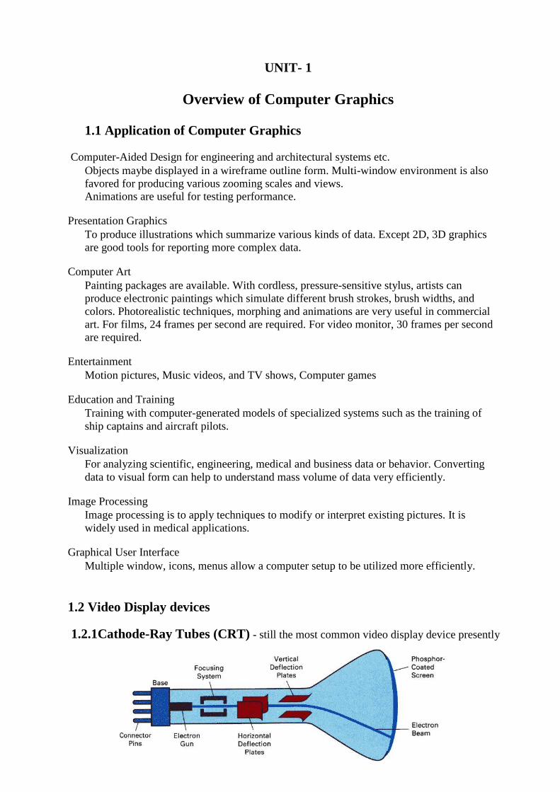
1.2.1Cathode-Ray Tubes (CRT) - still the most common video display device presently

Electrostatic deflection of the electron beam in a CRT An electron gun emits a beam of electrons, which passes through focusing and deflection

systems and hits on the phosphor-coated screen. The number of points displayed on a CRT is

referred to as resolutions (eg. 1024x768). Different phosphors emit small light spots of

different colors, which can combine to form a range of colors. A common methodology for

color CRT display is the Shadow-mask meth

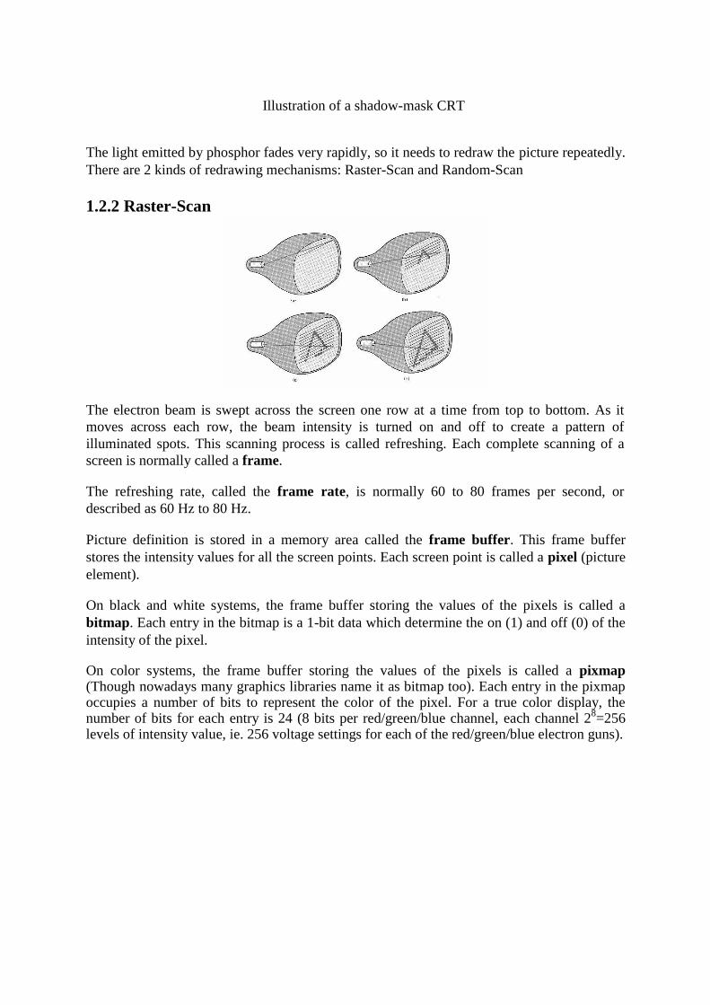
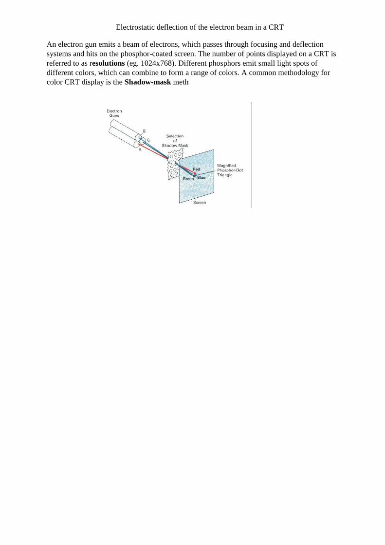
Illustration of a shadow-mask CRT

The light emitted by phosphor fades very rapidly, so it needs to redraw the picture repeatedly.

There are 2 kinds of redrawing mechanisms: Raster-Scan and Random-Scan

1.2.2 Raster-Scan

The electron beam is swept across the screen one row at a time from top to bottom. As it

moves across each row, the beam intensity is turned on and off to create a pattern of

illuminated spots. This scanning process is called refreshing. Each complete scanning of a

screen is normally called a frame. The refreshing rate, called the frame rate, is normally 60 to 80 frames per second, or

described as 60 Hz to 80 Hz. Picture definition is stored in a memory area called the frame buffer. This frame buffer

stores the intensity values for all the screen points. Each screen point is called a pixel (picture

element). On black and white systems, the frame buffer storing the values of the pixels is called a

bitmap. Each entry in the bitmap is a 1-bit data which determine the on (1) and off (0) of the

intensity of the pixel. On color systems, the frame buffer storing the values of the pixels is called a pixmap (Though nowadays many graphics libraries name it as bitmap too). Each entry in the pixmap occupies a number of bits to represent the color of the pixel. For a true color display, the number of bits for each entry is 24 (8 bits per red/green/blue channel, each channel 2

8=256

levels of intensity value, ie. 256 voltage settings for each of the red/green/blue electron guns).

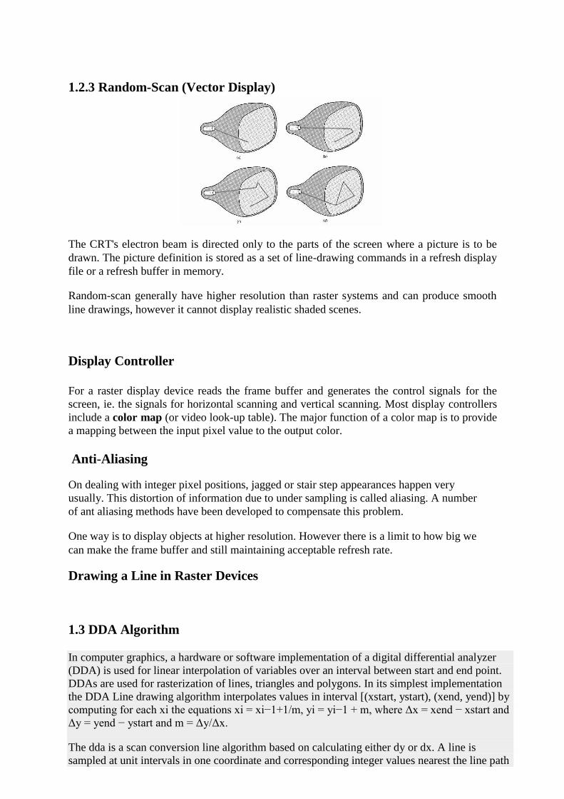
1.2.3 Random-Scan (Vector Display) The CRT's electron beam is directed only to the parts of the screen where a picture is to be

drawn. The picture definition is stored as a set of line-drawing commands in a refresh display

file or a refresh buffer in memory. Random-scan generally have higher resolution than raster systems and can produce smooth

line drawings, however it cannot display realistic shaded scenes.

Display Controller

For a raster display device reads the frame buffer and generates the control signals for the

screen, ie. the signals for horizontal scanning and vertical scanning. Most display controllers

include a color map (or video look-up table). The major function of a color map is to provide

a mapping between the input pixel value to the output color.

Anti-Aliasing On dealing with integer pixel positions, jagged or stair step appearances happen very

usually. This distortion of information due to under sampling is called aliasing. A number

of ant aliasing methods have been developed to compensate this problem. One way is to display objects at higher resolution. However there is a limit to how big we

can make the frame buffer and still maintaining acceptable refresh rate.

Drawing a Line in Raster Devices

1.3 DDA Algorithm

In computer graphics, a hardware or software implementation of a digital differential analyzer

(DDA) is used for linear interpolation of variables over an interval between start and end point.

DDAs are used for rasterization of lines, triangles and polygons. In its simplest implementation

the DDA Line drawing algorithm interpolates values in interval [(xstart, ystart), (xend, yend)] by

computing for each xi the equations xi = xi−1+1/m, yi = yi−1 + m, where Δx = xend − xstart and

Δy = yend − ystart and m = Δy/Δx.

The dda is a scan conversion line algorithm based on calculating either dy or dx. A line is

sampled at unit intervals in one coordinate and corresponding integer values nearest the line path

are determined for other coordinates.

Considering a line with positive slope, if the slope is less than or equal to 1, we sample at unit x

intervals (dx=1) and compute successive y values as

Subscript k takes integer values starting from 0, for the 1st point and increases by until endpoint

is reached. y value is rounded off to nearest integer to correspond to a screen pixel.

For lines with slope greater than 1, we reverse the role of x and y i.e. we sample at dy=1 and

calculate consecutive x values as

Similar calculations are carried out to determine pixel positions along a line with negative slope.

Thus, if the absolute value of the slope is less than 1, we set dx=1 if i.e. the starting extreme

point is at the left.

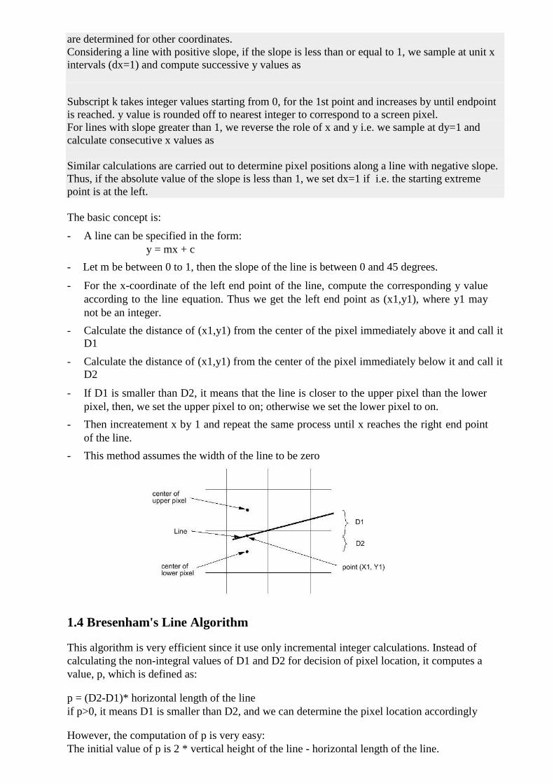
The basic concept is: - A line can be specified in the form:

y = mx + c - Let m be between 0 to 1, then the slope of the line is between 0 and 45 degrees. - For the x-coordinate of the left end point of the line, compute the corresponding y value

according to the line equation. Thus we get the left end point as (x1,y1), where y1 may

not be an integer. - Calculate the distance of (x1,y1) from the center of the pixel immediately above it and call it

D1 - Calculate the distance of (x1,y1) from the center of the pixel immediately below it and call it

D2 - If D1 is smaller than D2, it means that the line is closer to the upper pixel than the lower

pixel, then, we set the upper pixel to on; otherwise we set the lower pixel to on. - Then increatement x by 1 and repeat the same process until x reaches the right end point

of the line. - This method assumes the width of the line to be zero

1.4 Bresenham's Line Algorithm This algorithm is very efficient since it use only incremental integer calculations. Instead of

calculating the non-integral values of D1 and D2 for decision of pixel location, it computes a

value, p, which is defined as: p = (D2-D1)* horizontal length of the line if p>0, it means D1 is smaller than D2, and we can determine the pixel location accordingly However, the computation of p is very easy: The initial value of p is 2 * vertical height of the line - horizontal length of the line.

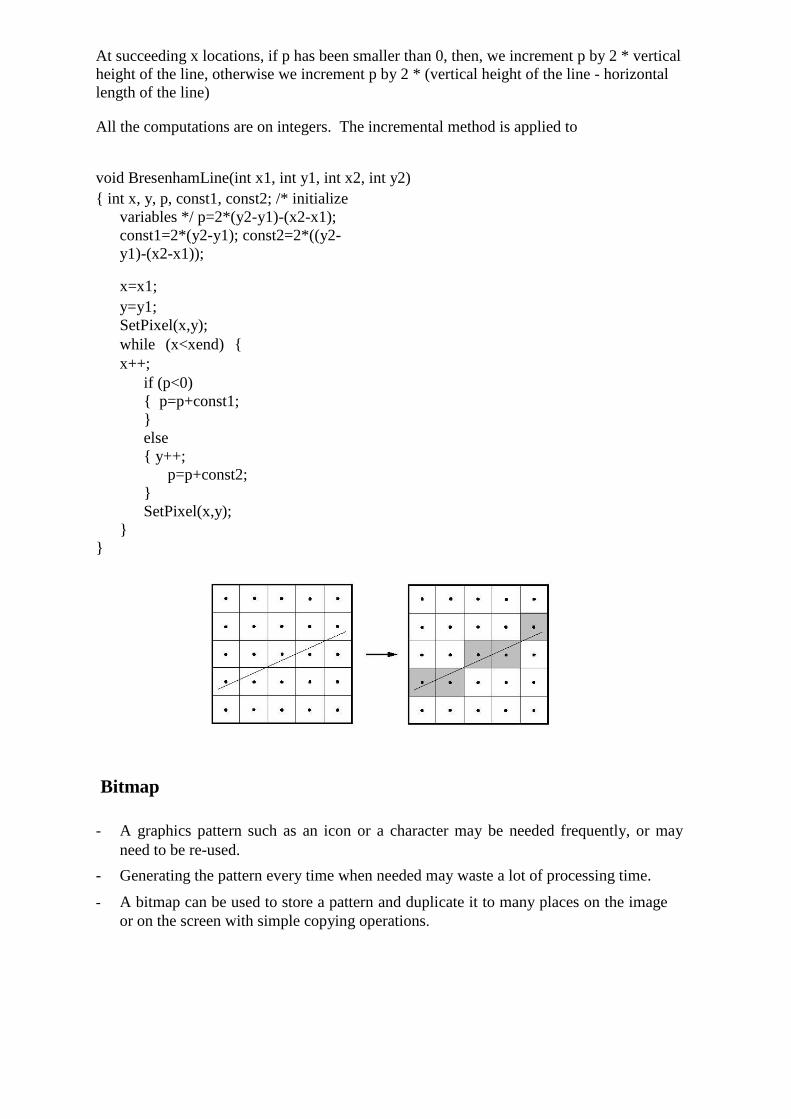
At succeeding x locations, if p has been smaller than 0, then, we increment p by 2 * vertical

height of the line, otherwise we increment p by 2 * (vertical height of the line - horizontal

length of the line) All the computations are on integers. The incremental method is applied to

void BresenhamLine(int x1, int y1, int x2, int y2) { int x, y, p, const1, const2; /* initialize

variables */ p=2*(y2-y1)-(x2-x1);

const1=2*(y2-y1); const2=2*((y2-

y1)-(x2-x1));

x=x1; y=y1;

SetPixel(x,y);

while (x<xend) {

x++; if (p<0)

{ p=p+const1;

}

else

{ y++;

p=p+const2; }

SetPixel(x,y);

}

}

Bitmap

- A graphics pattern such as an icon or a character may be needed frequently, or may

need to be re-used. - Generating the pattern every time when needed may waste a lot of processing time. - A bitmap can be used to store a pattern and duplicate it to many places on the image

or on the screen with simple copying operations.

1.5 Mid Point circle Algorithm

However, unsurprisingly this is not a brilliant solution!

Firstly, the resulting circle has large gaps where the slope approaches the vertical

Secondly, the calculations are not very efficient

The square (multiply) operations

The square root operation – try really hard to avoid these!

We need a more efficient, more accurate solution.

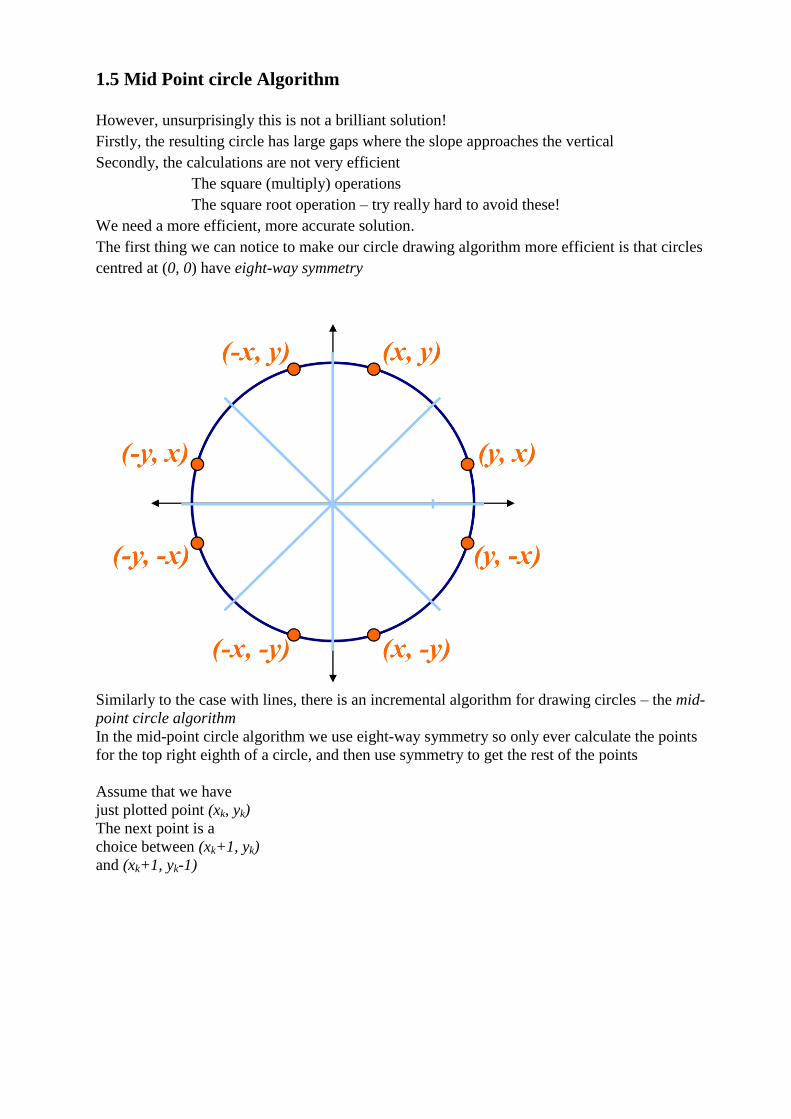
The first thing we can notice to make our circle drawing algorithm more efficient is that circles

centred at (0, 0) have eight-way symmetry

Similarly to the case with lines, there is an incremental algorithm for drawing circles – the mid-

point circle algorithm

In the mid-point circle algorithm we use eight-way symmetry so only ever calculate the points

for the top right eighth of a circle, and then use symmetry to get the rest of the points

Assume that we have

just plotted point (xk, yk)

The next point is a

choice between (xk+1, yk)

and (xk+1, yk-1)

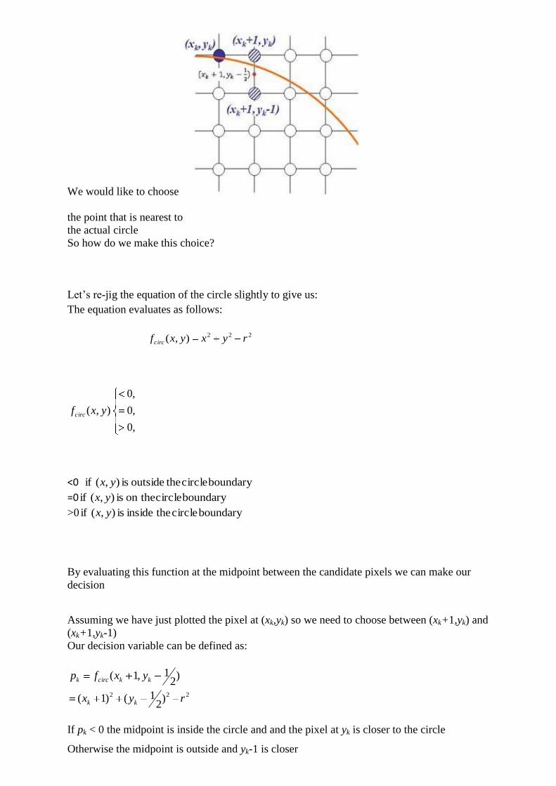
We would like to choose

the point that is nearest to

the actual circle

So how do we make this choice?

Let’s re-jig the equation of the circle slightly to give us:

The equation evaluates as follows:

222),( ryxyxfcirc

,0

,0

,0

),( yxfcirc

<0 boundary circle theoutside is ),( if yx

=0 boundary circle on the is ),( if yx

>0 boundary circle theinside is ),( if yx

By evaluating this function at the midpoint between the candidate pixels we can make our

decision

Assuming we have just plotted the pixel at (xk,yk) so we need to choose between (xk+1,yk) and

(xk+1,yk-1)

Our decision variable can be defined as:

)2

1,1( kkcirck yxfp

222 )2

1()1( ryx kk

If pk < 0 the midpoint is inside the circle and and the pixel at yk is closer to the circle

Otherwise the midpoint is outside and yk-1 is closer

To ensure things are as efficient as possible we can do all of our calculations incrementally

First consider:

21,1 111 kkcirck yxfp

22

1

2

21]1)1[( ryx kk

1)()()1(2 1

22

11 kkkkkkk yyyyxpp

where yk+1 is either yk or yk-1 depending on the sign of pk

The first decision variable is given as:

)2

1,1(0 rfp circ

22)2

1(1 rr

r4

5

Then if pk < 0 then the next decision variable is given as:

12 11 kkk xpp

If pk > 0 then the decision variable is:

1212 11 kkkk yxpp

Input radius r and circle centre (xc, yc), then set the coordinates for the first point on the

circumference of a circle centred on the origin as:

),0(),( 00 ryx

• Calculate the initial value of the decision parameter as:

rp4

50

• Starting with k = 0 at each position xk, perform the following test. If pk < 0, the next point

along the circle centred on (0, 0) is (xk+1, yk) and:

12 11 kkk xpp

Otherwise the next point along the circle is (xk+1, yk-1) and:

111 212 kkkk yxpp

Determine symmetry points in the other seven octants

Move each calculated pixel position (x, y) onto the circular path centred at (xc, yc) to plot the

coordinate values:

cxxx cyyy

Repeat steps 3 to 5 until x >= y

To see the mid-point circle algorithm in action lets use it to draw a circle centred at (0,0) with

radius 10

UNIT_-2

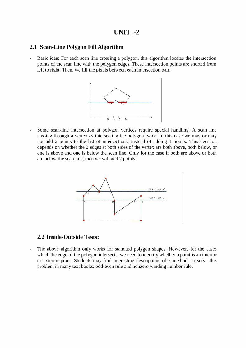
2.1 Scan-Line Polygon Fill Algorithm - Basic idea: For each scan line crossing a polygon, this algorithm locates the intersection

points of the scan line with the polygon edges. These intersection points are shorted from

left to right. Then, we fill the pixels between each intersection pair. - Some scan-line intersection at polygon vertices require special handling. A scan line

passing through a vertex as intersecting the polygon twice. In this case we may or may

not add 2 points to the list of intersections, instead of adding 1 points. This decision

depends on whether the 2 edges at both sides of the vertex are both above, both below, or

one is above and one is below the scan line. Only for the case if both are above or both

are below the scan line, then we will add 2 points.

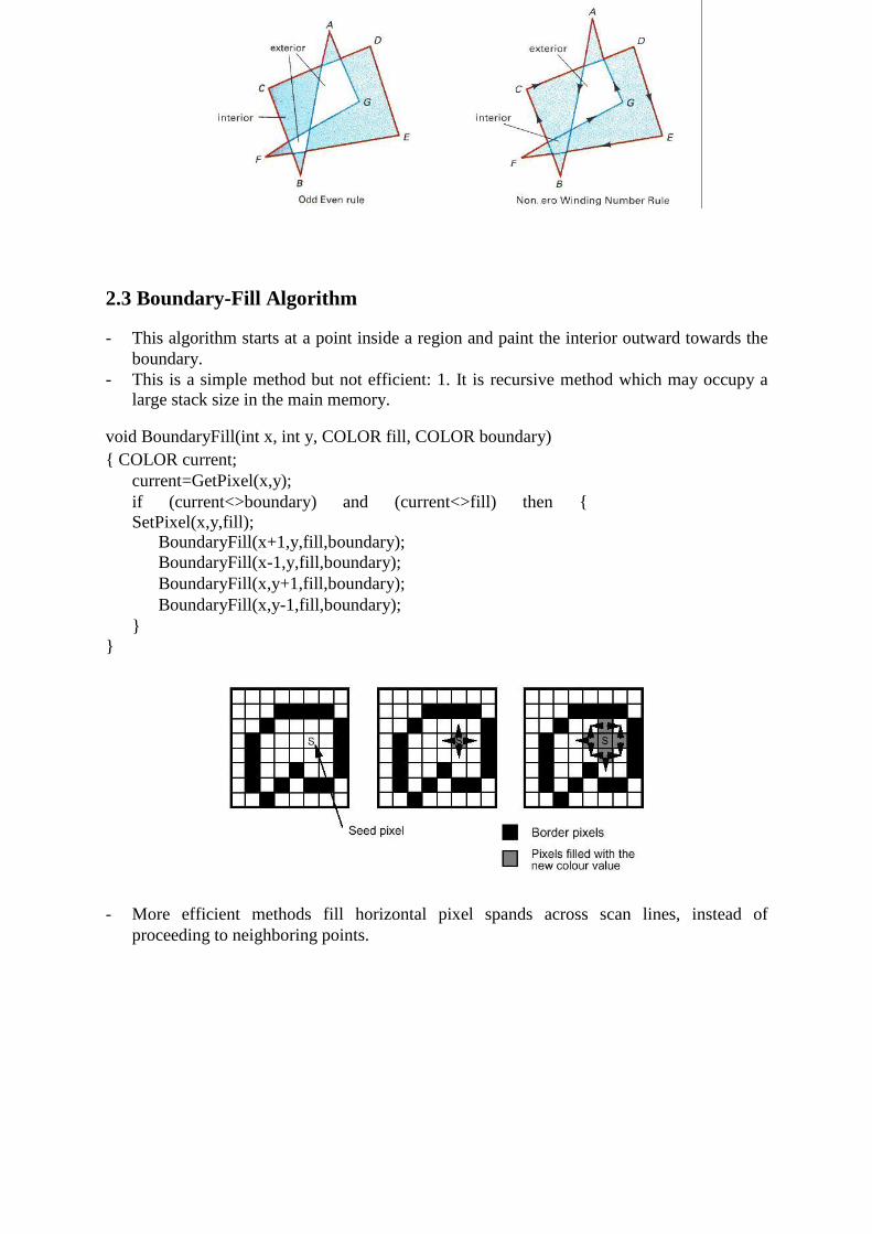
2.2 Inside-Outside Tests:

- The above algorithm only works for standard polygon shapes. However, for the cases

which the edge of the polygon intersects, we need to identify whether a point is an interior

or exterior point. Students may find interesting descriptions of 2 methods to solve this

problem in many text books: odd-even rule and nonzero winding number rule.

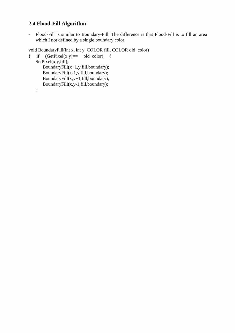
2.3 Boundary-Fill Algorithm - This algorithm starts at a point inside a region and paint the interior outward towards the

boundary. - This is a simple method but not efficient: 1. It is recursive method which may occupy a

large stack size in the main memory. void BoundaryFill(int x, int y, COLOR fill, COLOR boundary) { COLOR current;

current=GetPixel(x,y); if (current<>boundary) and (current<>fill) then {

SetPixel(x,y,fill); BoundaryFill(x+1,y,fill,boundary); BoundaryFill(x-1,y,fill,boundary);

BoundaryFill(x,y+1,fill,boundary);

BoundaryFill(x,y-1,fill,boundary); }

}

- More efficient methods fill horizontal pixel spands across scan lines, instead of

proceeding to neighboring points.

2.4 Flood-Fill Algorithm - Flood-Fill is similar to Boundary-Fill. The difference is that Flood-Fill is to fill an area

which I not defined by a single boundary color. void BoundaryFill(int x, int y, COLOR fill, COLOR old_color) { if (GetPixel(x,y)== old_color) {

SetPixel(x,y,fill);

BoundaryFill(x+1,y,fill,boundary);

BoundaryFill(x-1,y,fill,boundary);

BoundaryFill(x,y+1,fill,boundary);

BoundaryFill(x,y-1,fill,boundary); }

UNIT 3

Two Dimensional Transformations In many applications, changes in orientations, size, and shape are accomplished with

geometric transformations that alter the coordinate descriptions of objects. Basic geometric transformations are:

Translation Rotation Scaling

Other transformations:

Reflection

Shear

3.1 Basic Transformations Translation We translate a 2D point by adding translation distances, tx and ty, to the original coordinate

position (x,y):

x' = x + tx, y' = y + ty Alternatively, translation can also be specified by the following transformation matrix:

1 0 t x

0 1 t

y

0 0 1 Then we can rewrite the formula as:

x' 1 0 t x x

=

1

y' 0 t y

y

1 0 0 1 1

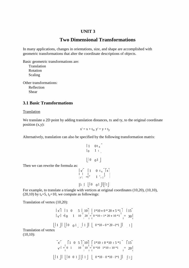
For example, to translate a triangle with vertices at original coordinates (10,20), (10,10), (20,10) by tx=5, ty=10, we compute as followings: Translation of vertex (10,20):

x' 1 0 5 10 1*10 0 * 20 5 *1 15

y' = 0 1 10 20 = 0 *10 1* 20 10 *1 = 30

1 0 0 1 1 0 *10 0 * 20 1*1 1

Translation of vertex

(10,10):

x' 1 0 5 10 1*10 0 *10 5 *1 15

y' = 0 1 10 10 = 0 *10 1*10 10 *1 = 20

1 0 0 1 1 0 *10 0 *10 1*1 1

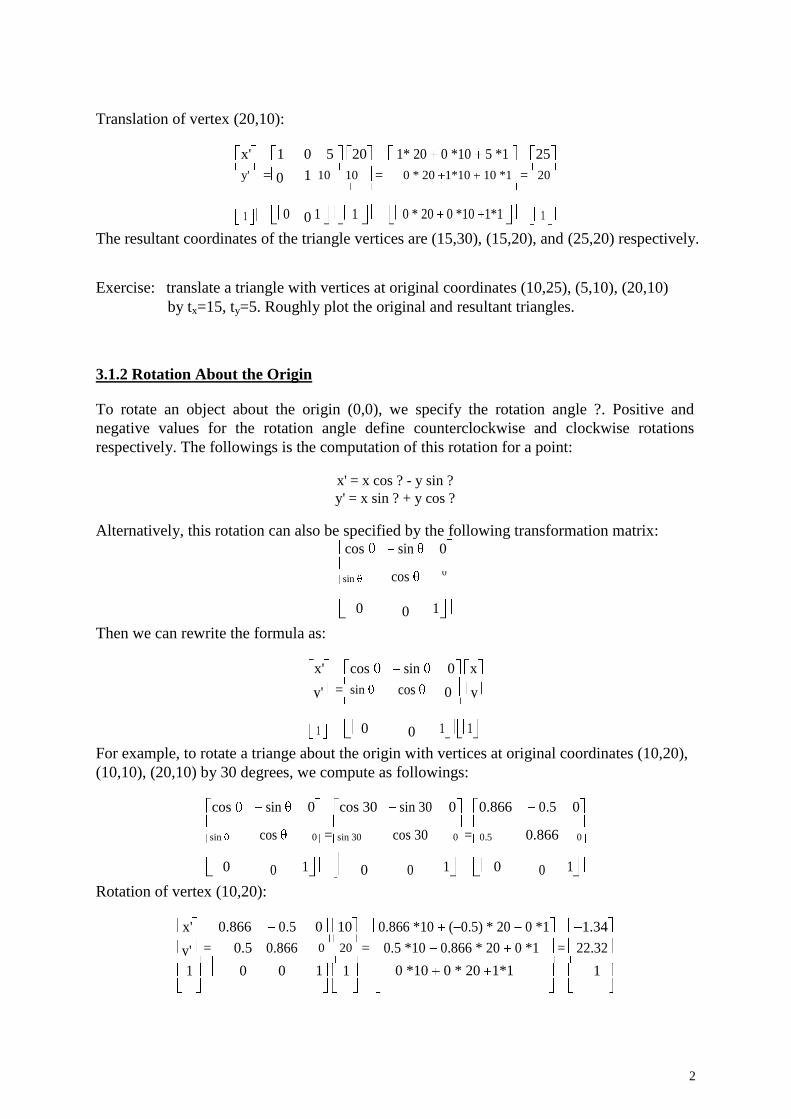
Translation of vertex (20,10):

x' 1 0 5 20 1* 20 0 *10 5 *1 25

y' = 0 1 10 10 = 0 * 20 1*10 10 *1 = 20

1 0 0 1 1 0 * 20 0 *10 1*1 1 The resultant coordinates of the triangle vertices are (15,30), (15,20), and (25,20) respectively. Exercise: translate a triangle with vertices at original coordinates (10,25), (5,10), (20,10)

by tx=15, ty=5. Roughly plot the original and resultant triangles.

3.1.2 Rotation About the Origin To rotate an object about the origin (0,0), we specify the rotation angle ?. Positive and

negative values for the rotation angle define counterclockwise and clockwise rotations

respectively. The followings is the computation of this rotation for a point:

x' = x cos ? - y sin ?

y' = x sin ? + y cos ? Alternatively, this rotation can also be specified by the following transformation matrix:

cos sin 0

cos

sin 0

0 0 1

Then we can rewrite the formula as:

x' cos sin 0 x

y' = sin cos 0 y

1 0 0 1 1 For example, to rotate a triange about the origin with vertices at original coordinates (10,20),

(10,10), (20,10) by 30 degrees, we compute as followings:

cos sin 0 cos 30 sin 30 0 0.866 0.5 0

cos

=

cos 30

=

0.866

sin 0 sin 30 0 0.5 0

0 0 1 0 0 1 0 0 1

Rotation of vertex (10,20):

x' 0.866 0.5 0 10 0.866 *10 ( 0.5) * 20 0 *1 1.34

y' = 0.5 0.866 0 20 = 0.5 *10 0.866 * 20 0 *1 = 22.32 1 0 0 1 1 0 *10 0 * 20 1*1 1

2

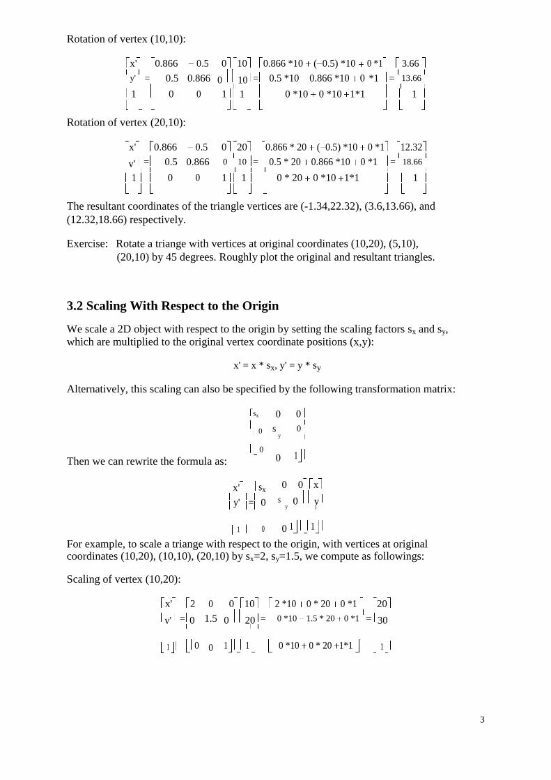
Rotation of vertex (10,10):

x' 0.866 0.5 0 10 0.866 *10 ( 0.5) *10 0 *1 3.66

y' = 0.5 0.866 0 10 = 0.5 *10 0.866 *10 0 *1 = 13.66 1 0 0 1 1 0 *10 0 *10 1*1 1

Rotation of vertex (20,10):

x' 0.866 0.5 0 20 0.866 * 20 ( 0.5) *10 0 *1 12.32

y' = 0.5 0.866 0 10 = 0.5 * 20 0.866 *10 0 *1 = 18.66 1 0 0 1 1 0 * 20 0 *10 1*1 1

The resultant coordinates of the triangle vertices are (-1.34,22.32), (3.6,13.66), and

(12.32,18.66) respectively. Exercise: Rotate a triange with vertices at original coordinates (10,20), (5,10),

(20,10) by 45 degrees. Roughly plot the original and resultant triangles.

3.2 Scaling With Respect to the Origin We scale a 2D object with respect to the origin by setting the scaling factors sx and sy,

which are multiplied to the original vertex coordinate positions (x,y):

x' = x * sx, y' = y * sy Alternatively, this scaling can also be specified by the following transformation matrix:

sx

0

0 Then we can rewrite the formula as:

x' sx

y'

=

0

1 0

0 0

s y 0

0 1

0 0 x

s y 0 y

0 1 1

For example, to scale a triange with respect to the origin, with vertices at original coordinates (10,20), (10,10), (20,10) by sx=2, sy=1.5, we compute as followings: Scaling of vertex (10,20):

x' 2 0 0 10 2 *10 0 * 20 0 *1 20

y' = 0 1.5 0 20 = 0 *10 1.5 * 20 0 *1 = 30

1 0 0 1 1 0 *10 0 * 20 1*1 1

3

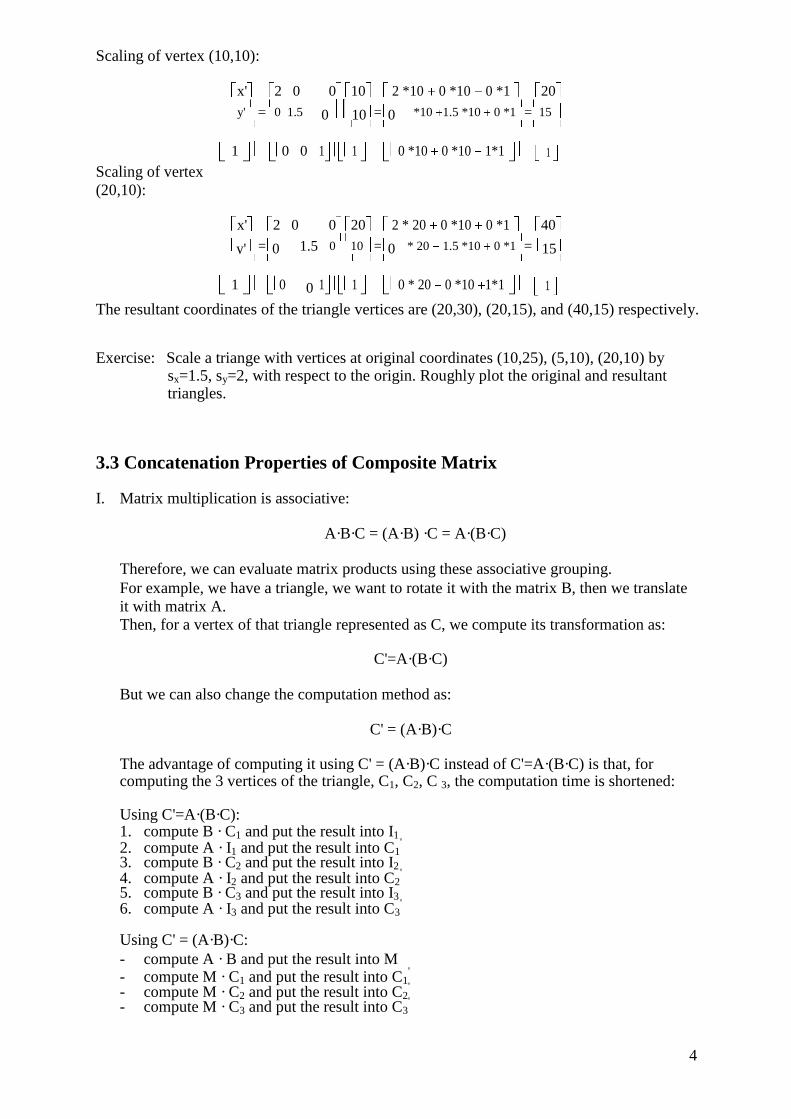
Scaling of vertex (10,10):

x' 2 0 0 10 2 *10 0 *10 0 *1 20

y' = 0 1.5 0 10 = 0 *10 1.5 *10 0 *1 = 15

1 0 0 1 1 0 *10 0 *10 1*1 1

Scaling of vertex

(20,10):

x' 2 0 0 20 2 * 20 0 *10 0 *1 40

y' = 0 1.5 0 10 = 0 * 20 1.5 *10 0 *1 = 15

1 0 0 1 1 0 * 20 0 *10 1*1 1 The resultant coordinates of the triangle vertices are (20,30), (20,15), and (40,15) respectively. Exercise: Scale a triange with vertices at original coordinates (10,25), (5,10), (20,10) by

sx=1.5, sy=2, with respect to the origin. Roughly plot the original and resultant triangles.

3.3 Concatenation Properties of Composite Matrix I. Matrix multiplication is associative:

A·B·C = (A·B) ·C = A·(B·C)

Therefore, we can evaluate matrix products using these associative grouping. For example, we have a triangle, we want to rotate it with the matrix B, then we translate

it with matrix A.

Then, for a vertex of that triangle represented as C, we compute its transformation as:

C'=A·(B·C)

But we can also change the computation method as:

C' = (A·B)·C

The advantage of computing it using C' = (A·B)·C instead of C'=A·(B·C) is that, for computing the 3 vertices of the triangle, C1, C2, C 3, the computation time is shortened:

Using C'=A·(B·C): 1. compute B · C1 and put the result into I1 2. compute A · I1 and put the result into C1

'

3. compute B · C2 and put the result into I2 4. compute A · I2 and put the result into C2

'

5. compute B · C3 and put the result into I3 6. compute A · I3 and put the result into C3

'

Using C' = (A·B)·C: - compute A · B and put the result into M - compute M · C1 and put the result into C1

'

- compute M · C2 and put the result into C2'

- compute M · C3 and put the result into C3'

4

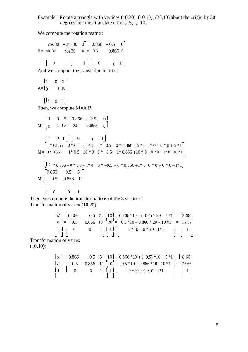
Example: Rotate a triangle with vertices (10,20), (10,10), (20,10) about the origin by 30 degrees and then translate it by tx=5, ty=10,

We compute the rotation matrix:

cos 30 sin 30 0 0.866 0.5 0

B = sin 30 cos 30 0 = 0.5 0.866 0

0 0 1 0 0 1

And we compute the translation matrix:

1 0 5

A= 0 1 10

0 0 1

Then, we compute M=A·B

1 0 5 0.866 0.5 0

M= 0 1 10 · 0.5 0.866 0

0 0 1 0 0 1

1* 0.866 0 * 0.5 5 * 0 1* 0.5 0 * 0.866 5 * 0 1* 0 0 * 0 5 *1

M= 0 * 0.866 1* 0.5 10 * 0 0 * 0.5 1* 0.866 10 * 0 0 * 0 1* 0 10 *1

0 * 0.866 0 * 0.5 1* 0 0 * 0.5 0 * 0.866 1* 0 0 * 0 0 * 0 1*1

0.866 0.5 5

M= 0.5 0.866 10

0 0 1 Then, we compute the transformations of the 3 vertices: Transformation of vertex (10,20):

x' 0.866 0.5 5 10 0.866 *10 ( 0.5) * 20 5 *1 3.66

y' = 0.5 0.866 10 20 = 0.5 *10 0.866 * 20 10 *1 = 32.32 1 0 0 1 1 0 *10 0 * 20 1*1 1

Transformation of vertex

(10,10):

x' 0.866 0.5 5 10 0.866 *10 ( 0.5) *10 5 *1 8.66

y' = 0.5 0.866 10 10 = 0.5 *10 0.866 *10 10 *1 = 23.66 1 0 0 1 1 0 *10 0 *10 1*1 1

5

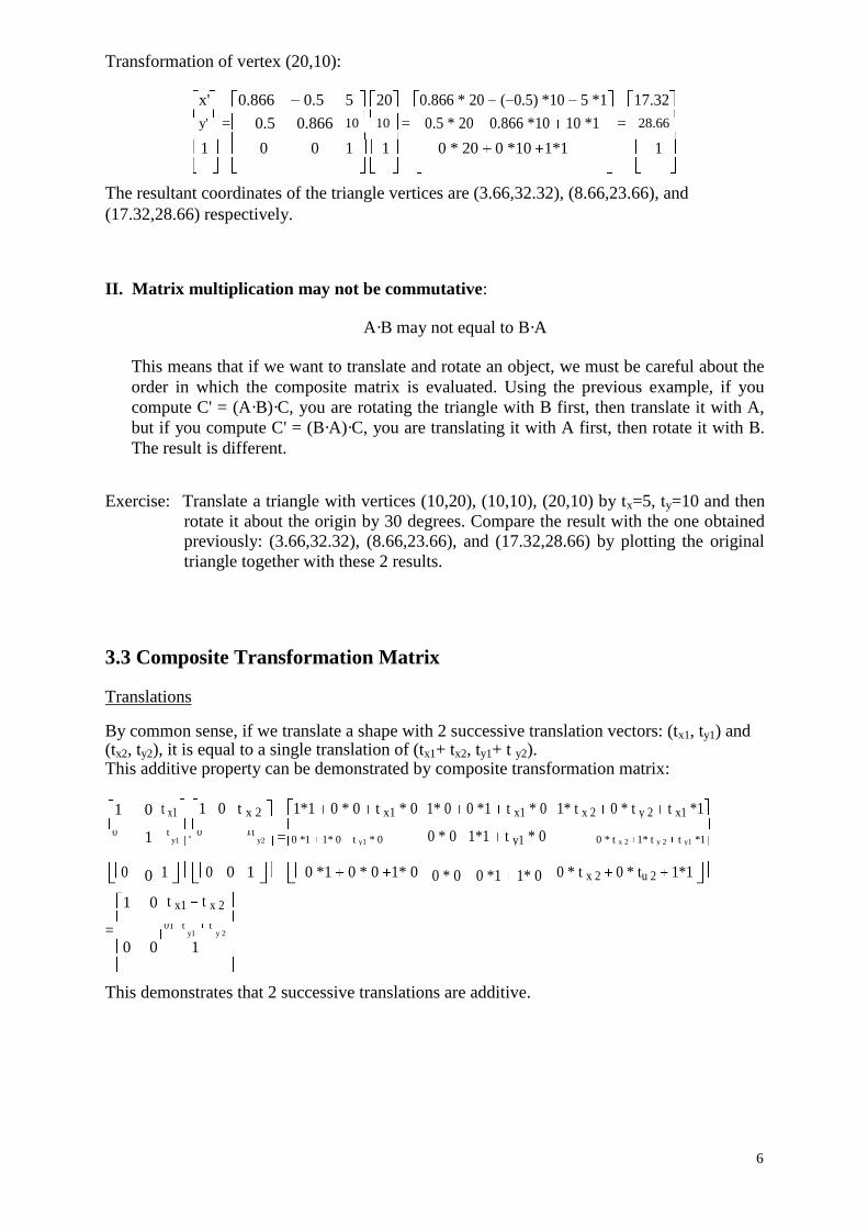
Transformation of vertex (20,10):

x' 0.866 0.5 5 20 0.866 * 20 ( 0.5) *10 5 *1 17.32

y' = 0.5 0.866 10 10 = 0.5 * 20 0.866 *10 10 *1 = 28.66 1 0 0 1 1 0 * 20 0 *10 1*1 1

The resultant coordinates of the triangle vertices are (3.66,32.32), (8.66,23.66), and

(17.32,28.66) respectively.

II. Matrix multiplication may not be commutative:

A·B may not equal to B·A

This means that if we want to translate and rotate an object, we must be careful about the

order in which the composite matrix is evaluated. Using the previous example, if you

compute C' = (A·B)·C, you are rotating the triangle with B first, then translate it with A,

but if you compute C' = (B·A)·C, you are translating it with A first, then rotate it with B.

The result is different. Exercise: Translate a triangle with vertices (10,20), (10,10), (20,10) by tx=5, ty=10 and then

rotate it about the origin by 30 degrees. Compare the result with the one obtained

previously: (3.66,32.32), (8.66,23.66), and (17.32,28.66) by plotting the original

triangle together with these 2 results. 3.3 Composite Transformation Matrix Translations By common sense, if we translate a shape with 2 successive translation vectors: (tx1, ty1) and (tx2, ty2), it is equal to a single translation of (tx1+ tx2, ty1+ t y2). This additive property can be demonstrated by composite transformation matrix:

1 0 t x1 1 0 t x 2 1*1 0 * 0 t x1 * 0 1* 0 0 *1 t x1 * 0 1* t x 2 0 * t y 2 t x1 *1

1

·

=

0 * 0 1*1 t y1 * 0

0 t y1 0

1t y2 0 *1 1* 0 t y1 * 0 0 * t x 2 1* t y 2 t y1 *1

0 0 1 0 0 1 0 *1 0 * 0 1* 0 0 * 0 0 *1 1* 0 0 * t x 2 0 * tu 2 1*1

1 0 t x1 t x 2

=

01 t y1

t y 2

0 0 1

This demonstrates that 2 successive translations are additive. 6

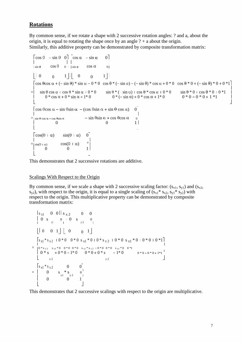
Rotations By common sense, if we rotate a shape with 2 successive rotation angles: ? and a, about the

origin, it is equal to rotating the shape once by an angle ? + a about the origin. Similarly, this additive property can be demonstrated by composite transformation matrix: cos sin 0 cos sin 0

cos

cos

sin 0 · sin 0

0 0 1 0 0 1

cos cos ( sin ) * sin 0 * 0 cos * ( sin ) ( sin ) * cos 0 * 0 cos * 0 ( sin ) * 0 0 *1

=

sin cos cos * sin 0 * 0 sin * ( sin ) cos * cos 0 * 0 sin * 0 cos * 0 0 *1

0 * cos 0 * sin 1* 0 0 * ( sin ) 0 * cos 1* 0 0 * 0 0 * 0 1 *1

cos cos sin sin (cos sin sin cos ) 0

=

sin sin cos cos

sin cos cos sin 0

0 0 1

cos( ) sin( ) 0

=

cos( )

sin( ) 0

0 0 1

This demonstrates that 2 successive rotations are additive.

Scalings With Respect to the Origin By common sense, if we scale a shape with 2 successive scaling factor: (sx1, sy1) and (sx2, sy2), with respect to the origin, it is equal to a single scaling of (sx1* sx2, sy1* sy2) with respect to the origin. This multiplicative property can be demonstrated by composite transformation matrix:

s x1 0 0 s x 2 0 0

0 s y1

0 · 0 s y 2

0

0 0 1 0 0 1

s x1 * s x 2 0 * 0 0 * 0 s x1 * 0 0 * s y 2 0 * 0 s x1 * 0 0 * 0 0 *1

=

0 * s x 2 s y1 * 0 0 * 0 0 * 0 s y1 * s y 2 0 * 0 0 * 0 s y1 * 0 0 *1

0 * s

x 2

0 * 0 1* 0 0 * 0 0 * s

y 2

1* 0 0 * 0 0 * 0 1*1

s x1 * s x 2 0 0

= 0 s y1

* s y 2

0

0 0 1

This demonstrates that 2 successive scalings with respect to the origin are multiplicative. 7

3.4 General Pivot-Point Rotation Rotation about an arbitrary pivot point is not as simple as rotation about the origin. The

procedure of rotation about an arbitrary pivot point is: - Translate the object so that the pivot-point position is moved to the origin. - Rotate the object about the origin. - Translate the object so that the pivot point is returned to its original position.

The corresponding composite transformation matrix is:

1 0 x r cos sin 0 1 0 x r

1

cos

1

0 y r sin 0 0

y r

0 0 1 0 0 1 0 0 1

cos sin

=

cos

sin

0 0

x r 1 0 x r

1

y r 0

y r

1 0 0 1

cos sin x r cos

=

cos x r sin

sin

0 0

y r sin x r

y r cos y r 1

3.5 General Fixed-Point Scaling Scaling with respect to an arbitrary fixed point is not as simple as scaling with respect to

the origin. The procedure of scaling with respect to an arbitrary fixed point is: 1. Translate the object so that the fixed point coincides with the origin. 2. Scale the object with respect to the origin. 3. Use the inverse translation of step 1 to return the object to its original position.

8

The corresponding composite transformation matrix is:

1 0 x f sx 0 0 1 0 x f s x 0 x f (1 s x )

1

0 sy

1

=

0 s y y f

0 y f 0 0

yf (1 s y )

0 0 1 0 0 1 0 0 1 0 0 1

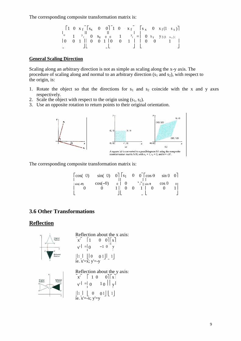
General Scaling Direction Scaling along an arbitrary direction is not as simple as scaling along the x-y axis. The procedure of scaling along and normal to an arbitrary direction (s1 and s2), with respect to the origin, is: 1. Rotate the object so that the directions for s1 and s2 coincide with the x and y axes

respectively. 2. Scale the object with respect to the origin using (s1, s2). 3. Use an opposite rotation to return points to their original orientation. The corresponding composite transformation matrix is:

cos( ) sin( ) 0 s1 0 0 cos sin 0

cos( )

0

cos

sin( ) 0 s

20 sin 0

0 0 1 0 0 1 0 0 1

3.6 Other Transformations Reflection

Reflection about the x axis: x' 1 0 0 x

y' = 0 1 0 y

1 0 0 1 1 ie. x'=x; y'=-y

Reflection about the y axis: x' 1 0 0 x

y' = 0 1 0 y

1 0 0 1 1 ie. x'=-x; y'=y

9

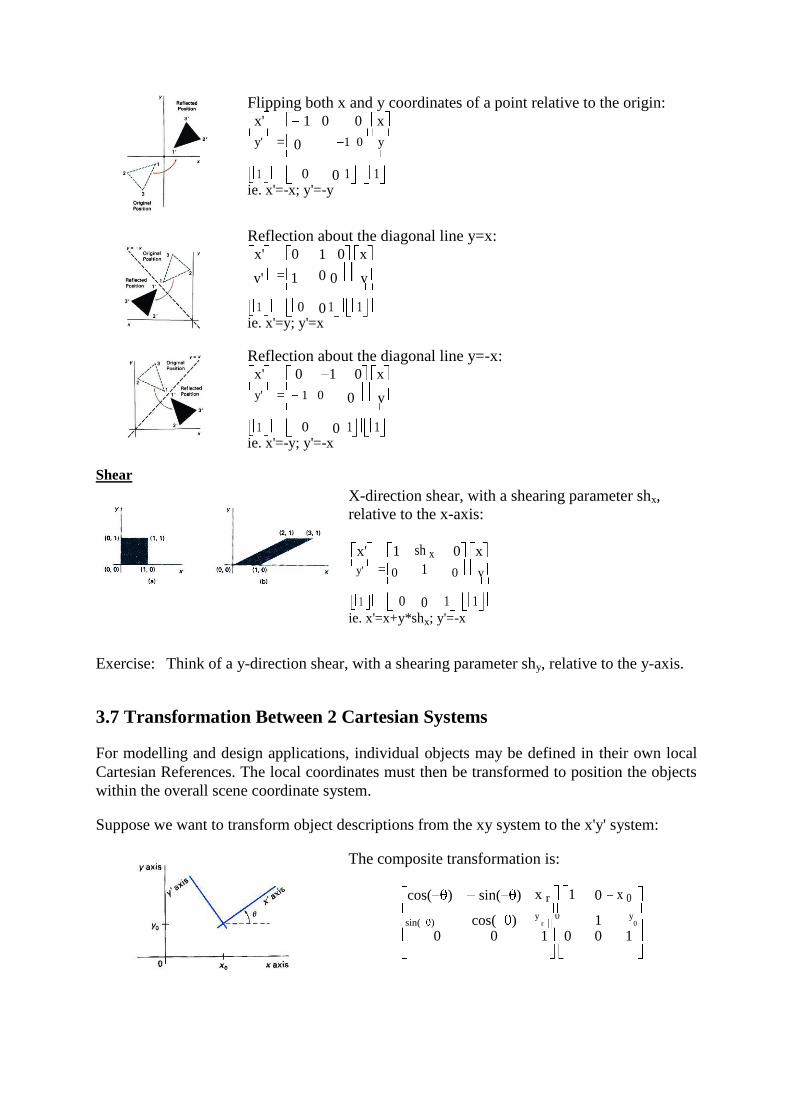
Flipping both x and y coordinates of a point relative to the origin: x' 1 0 0 x

y' = 0 1 0 y

1 0 0 1 1 ie. x'=-x; y'=-y

Reflection about the diagonal line y=x: x' 0 1 0 x

y' = 1 0 0 y

1 0 0 1 1 ie. x'=y; y'=x

Reflection about the diagonal line y=-x: x' 0 1 0 x

y' = 1 0 0 y

1 0 0 1 1 ie. x'=-y; y'=-x

Shear

X-direction shear, with a shearing parameter shx,

relative to the x-axis:

x' 1 sh x 0 x

y' = 0 1 0 y

1 0 0 1 1 ie. x'=x+y*shx; y'=-x

Exercise: Think of a y-direction shear, with a shearing parameter shy, relative to the y-axis.

3.7 Transformation Between 2 Cartesian Systems For modelling and design applications, individual objects may be defined in their own local

Cartesian References. The local coordinates must then be transformed to position the objects

within the overall scene coordinate system. Suppose we want to transform object descriptions from the xy system to the x'y' system:

The composite transformation is:

cos( ) sin( ) x r 1 0 x 0

cos( )

1

sin( ) y r

0 y

0

0 0 1 0 0 1

UNIT -4

2-Dimensional viewing

4.1Images on the Screen

All objects in the real world have size. We use a unit of measure to describe both the size of an

object as well as the location of the object in the real world. For example, meters can be used to

specify both size and distance. When showing an image of an object on the screen, we use a

screen coordinate system that defines the location of the object in the same relative position as in

the real world. After we select the screen coordinate system, we change the picture to display

interior screen that means change it into screen coordinate system.

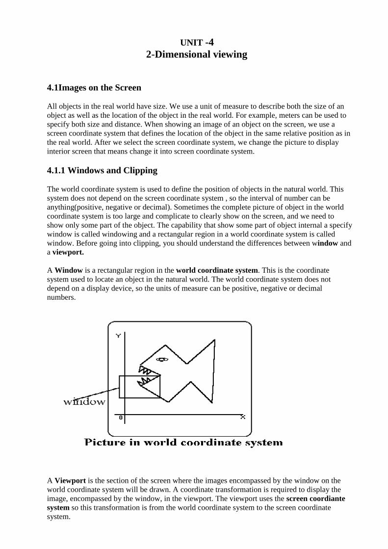
4.1.1 Windows and Clipping

The world coordinate system is used to define the position of objects in the natural world. This

system does not depend on the screen coordinate system , so the interval of number can be

anything(positive, negative or decimal). Sometimes the complete picture of object in the world

coordinate system is too large and complicate to clearly show on the screen, and we need to

show only some part of the object. The capability that show some part of object internal a specify

window is called windowing and a rectangular region in a world coordinate system is called

window. Before going into clipping, you should understand the differences between window and

a viewport.

A Window is a rectangular region in the world coordinate system. This is the coordinate

system used to locate an object in the natural world. The world coordinate system does not

depend on a display device, so the units of measure can be positive, negative or decimal

numbers.

A Viewport is the section of the screen where the images encompassed by the window on the

world coordinate system will be drawn. A coordinate transformation is required to display the

image, encompassed by the window, in the viewport. The viewport uses the screen coordiante

system so this transformation is from the world coordinate system to the screen coordinate

system.

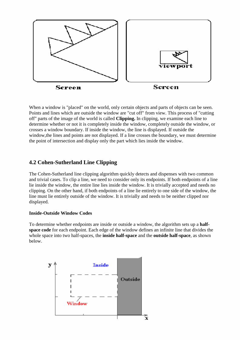
When a window is "placed" on the world, only certain objects and parts of objects can be seen.

Points and lines which are outside the window are "cut off" from view. This process of "cutting

off" parts of the image of the world is called Clipping. In clipping, we examine each line to

determine whether or not it is completely inside the window, completely outside the window, or

crosses a window boundary. If inside the window, the line is displayed. If outside the

window,the lines and points are not displayed. If a line crosses the boundary, we must determine

the point of intersection and display only the part which lies inside the window.

4.2 Cohen-Sutherland Line Clipping

The Cohen-Sutherland line clipping algorithm quickly detects and dispenses with two common

and trivial cases. To clip a line, we need to consider only its endpoints. If both endpoints of a line

lie inside the window, the entire line lies inside the window. It is trivially accepted and needs no

clipping. On the other hand, if both endpoints of a line lie entirely to one side of the window, the

line must lie entirely outside of the window. It is trivially and needs to be neither clipped nor

displayed.

Inside-Outside Window Codes

To determine whether endpoints are inside or outside a window, the algorithm sets up a half-

space code for each endpoint. Each edge of the window defines an infinite line that divides the

whole space into two half-spaces, the inside half-space and the outside half-space, as shown

below.

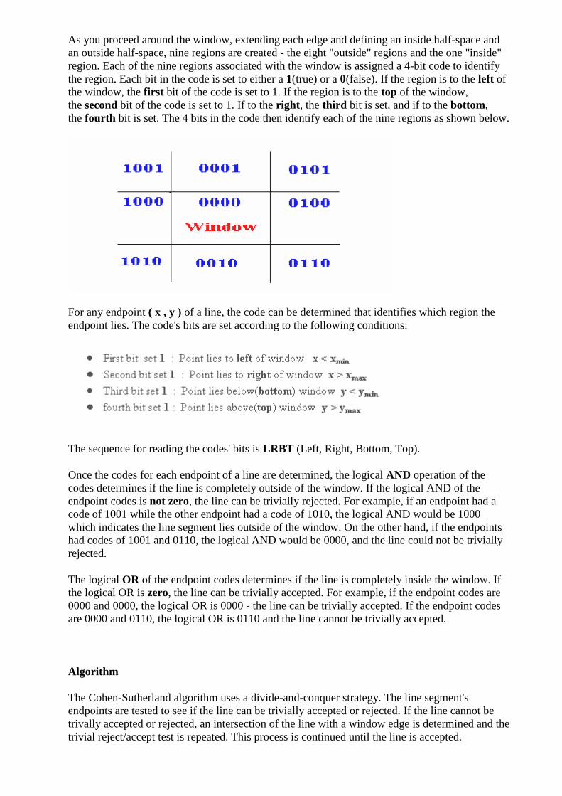
As you proceed around the window, extending each edge and defining an inside half-space and

an outside half-space, nine regions are created - the eight "outside" regions and the one "inside"

region. Each of the nine regions associated with the window is assigned a 4-bit code to identify

the region. Each bit in the code is set to either a 1(true) or a 0(false). If the region is to the left of

the window, the first bit of the code is set to 1. If the region is to the top of the window,

the second bit of the code is set to 1. If to the right, the third bit is set, and if to the bottom,

the fourth bit is set. The 4 bits in the code then identify each of the nine regions as shown below.

For any endpoint ( x , y ) of a line, the code can be determined that identifies which region the

endpoint lies. The code's bits are set according to the following conditions:

The sequence for reading the codes' bits is LRBT (Left, Right, Bottom, Top).

Once the codes for each endpoint of a line are determined, the logical AND operation of the

codes determines if the line is completely outside of the window. If the logical AND of the

endpoint codes is not zero, the line can be trivially rejected. For example, if an endpoint had a

code of 1001 while the other endpoint had a code of 1010, the logical AND would be 1000

which indicates the line segment lies outside of the window. On the other hand, if the endpoints

had codes of 1001 and 0110, the logical AND would be 0000, and the line could not be trivially

rejected.

The logical OR of the endpoint codes determines if the line is completely inside the window. If

the logical OR is zero, the line can be trivially accepted. For example, if the endpoint codes are

0000 and 0000, the logical OR is 0000 - the line can be trivially accepted. If the endpoint codes

are 0000 and 0110, the logical OR is 0110 and the line cannot be trivially accepted.

Algorithm

The Cohen-Sutherland algorithm uses a divide-and-conquer strategy. The line segment's

endpoints are tested to see if the line can be trivially accepted or rejected. If the line cannot be

trivally accepted or rejected, an intersection of the line with a window edge is determined and the

trivial reject/accept test is repeated. This process is continued until the line is accepted.

To perform the trivial acceptance and rejection tests, we extend the edges of the window to

divide the plane of the window into the nine regions. Each end point of the line segment is then

assigned the code of the region in which it lies.

1. Given a line segment with endpoint and

2. Compute the 4-bit codes for each endpoint.

If both codes are 0000,(bitwise OR of the codes yields 0000 ) line lies

completely inside the window: pass the endpoints to the draw routine.

If both codes have a 1 in the same bit position (bitwise AND of the codes is not 0000),

the line lies outside the window. It can be trivially rejected.

3. If a line cannot be trivially accepted or rejected, at least one of the two endpoints must lie

outside the window and the line segment crosses a window edge. This line must

be clipped at the window edge before being passed to the drawing routine.

4. Examine one of the endpoints, say . Read 's 4-bit code in order: Left-

to-Right, Bottom-to-Top.

5. When a set bit (1) is found, compute the intersection I of the corresponding window edge

with the line from to . Replace with I and repeat the algorithm.

4.3 Liang-Barsky Line Clipping

The ideas for clipping line of Liang-Barsky and Cyrus-Beck are the same. The only difference is

Liang-Barsky algorithm has been optimized for an upright rectangular clip window. So we will

study only the idea of Liang-Barsky.

Liang and Barsky have created an algorithm that uses floating-point arithmetic but finds the

appropriate end points with at most four computations. This algorithm uses the parametric

equations for a line and solves four inequalities to find the range of the parameter for which the

line is in the viewport.

Let P(x1,y1) , Q(x2,y2)be the line which we want to study. The parametric equation of the

line segment from gives x-values and y-values for every point in terms of a parameter that

ranges from 0 to 1. The equations are

and

We can see that when t = 0, the point computed is P(x1,y1); and when t = 1, the point computed

is Q(x2,y2).

Algorithm

1. Set and

2. Calculate the values of tL, tR, tT, and tB (tvalues).

o if or ignore it and go to the next edge

o otherwise classify the tvalue as entering or exiting value (using inner product to

classify)

o if t is entering value set ; if t is exiting value set

3. If then draw a line from (x1 + dx*tmin, y1 + dy*tmin) to (x1 + dx*tmax, y1

+ dy*tmax)

4. If the line crosses over the window, you will see (x1 + dx*tmin, y1 + dy*tmin) and (x1 +

dx*tmax, y1 + dy*tmax) are intersection between line and edge.

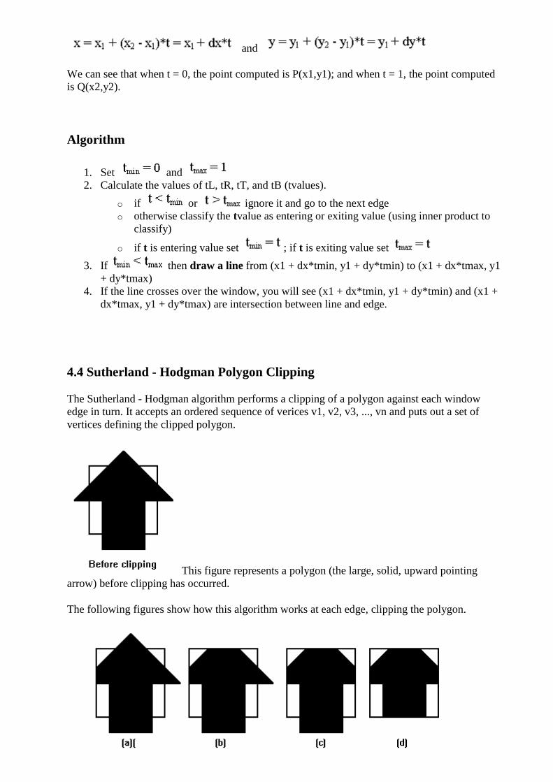
4.4 Sutherland - Hodgman Polygon Clipping

The Sutherland - Hodgman algorithm performs a clipping of a polygon against each window

edge in turn. It accepts an ordered sequence of verices v1, v2, v3, ..., vn and puts out a set of

vertices defining the clipped polygon.

This figure represents a polygon (the large, solid, upward pointing

arrow) before clipping has occurred.

The following figures show how this algorithm works at each edge, clipping the polygon.

a. Clipping against the left side of the clip window.

b. Clipping against the top side of the clip window.

c. Clipping against the right side of the clip window.

d. Clipping against the bottom side of the clip window.

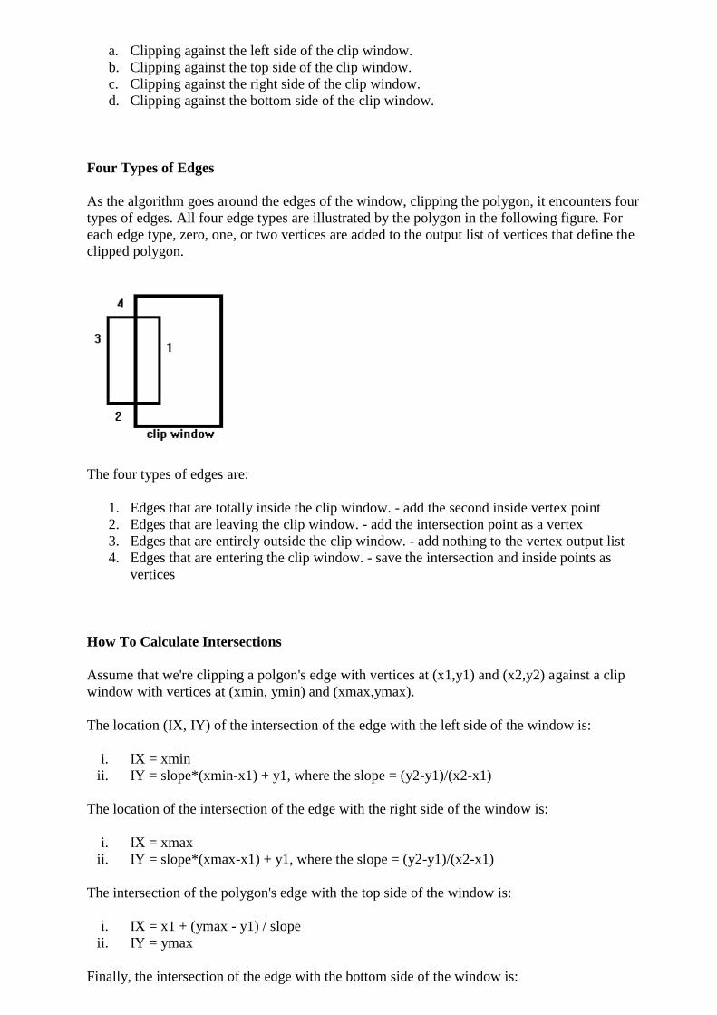
Four Types of Edges

As the algorithm goes around the edges of the window, clipping the polygon, it encounters four

types of edges. All four edge types are illustrated by the polygon in the following figure. For

each edge type, zero, one, or two vertices are added to the output list of vertices that define the

clipped polygon.

The four types of edges are:

1. Edges that are totally inside the clip window. - add the second inside vertex point

2. Edges that are leaving the clip window. - add the intersection point as a vertex

3. Edges that are entirely outside the clip window. - add nothing to the vertex output list

4. Edges that are entering the clip window. - save the intersection and inside points as

vertices

How To Calculate Intersections

Assume that we're clipping a polgon's edge with vertices at (x1,y1) and (x2,y2) against a clip

window with vertices at (xmin, ymin) and (xmax,ymax).

The location (IX, IY) of the intersection of the edge with the left side of the window is:

i. IX = xmin

ii. IY = slope*(xmin-x1) + y1, where the slope = (y2-y1)/(x2-x1)

The location of the intersection of the edge with the right side of the window is:

i. IX = xmax

ii. IY = slope*(xmax-x1) + y1, where the slope = (y2-y1)/(x2-x1)

The intersection of the polygon's edge with the top side of the window is:

i. IX = x1 + (ymax - y1) / slope

ii. IY = ymax

Finally, the intersection of the edge with the bottom side of the window is:

i. IX = x1 + (ymin - y1) / slope

ii. IY = ymin

Some Problems With This Algorithm

1. This algorithm does not work if the clip window is not convex.

2. If the polygon is not also convex, there may be some dangling edges.

UNIT-5

3D Object Representations

Methods: Polygon and Quadric surfaces: For simple Euclidean objects

Spline surfaces and construction: For curved surfaces

Procedural methods: Eg. Fractals, Particle systems

Physically based modeling methods

Octree Encoding

Isosurface displays, Volume rendering, etc. Classification:

Boundary Representations (B-reps) eg. Polygon facets and spline patches

Space-partitioning representations eg. Octree Representation Objects may also associate with other properties such as mass, volume, so as to determine

their response to stress and temperature etc.

5.1 Polygon Surfaces This method simplifies and speeds up the surface rendering and display of objects. For other 3D objection representations, they are often converted into polygon

surfaces before rendering. Polygon Mesh - Using a set of connected polygonally bounded planar surfaces to represent an object,

which may have curved surfaces or curved edges.

- The wireframe display of such object can be displayed quickly to give general

indication of the surface structure.

- Realistic renderings can be produced by interpolating shading patterns across the

polygon surfaces to eliminate or reduce the presence of polygon edge boundaries.

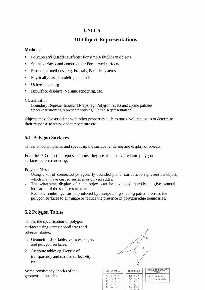
5.2 Polygon Tables This is the specification of polygon

surfaces using vertex coordinates and

other attributes: 1. Geometric data table: vertices, edges,

and polygon surfaces. 2. Attribute table: eg. Degree of

transparency and surface reflectivity

etc. Some consistency checks of the

geometric data table:

Every vertex is listed as an endpoint

for at least 2 edges

Every edge is part of at least one polygon

Every polygon is closed

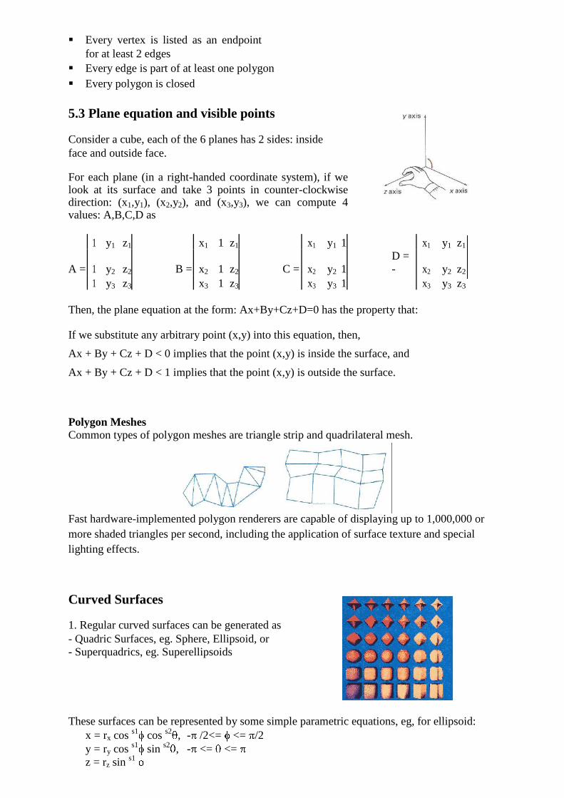
5.3 Plane equation and visible points Consider a cube, each of the 6 planes has 2 sides: inside

face and outside face. For each plane (in a right-handed coordinate system), if we look at its surface and take 3 points in counter-clockwise direction: (x1,y1), (x2,y2), and (x3,y3), we can compute 4 values: A,B,C,D as

1 y1 z1 x1 1 z1 x1 y1 1 x1 y1 z1

A = 1 y2 z2 B = x2 1 z2 C = x2 y2 1

D =

- x2 y2 z2

1 y3 z3 x3 1 z3 x3 y3 1 x3 y3 z3

Then, the plane equation at the form: Ax+By+Cz+D=0 has the property that: If we substitute any arbitrary point (x,y) into this equation, then, Ax + By + Cz + D < 0 implies that the point (x,y) is inside the surface, and Ax + By + Cz + D < 1 implies that the point (x,y) is outside the surface.

Polygon Meshes

Common types of polygon meshes are triangle strip and quadrilateral mesh.

Fast hardware-implemented polygon renderers are capable of displaying up to 1,000,000 or

more shaded triangles per second, including the application of surface texture and special

lighting effects.

Curved Surfaces 1. Regular curved surfaces can be generated as - Quadric Surfaces, eg. Sphere, Ellipsoid, or - Superquadrics, eg. Superellipsoids

These surfaces can be represented by some simple parametric equations, eg, for ellipsoid:

x = rx cos s1

cos s2

, - /2<= <= /2

y = ry cos s1

sin s2

, - <= <=

z = rz sin s1

Where s1, rx, ry, and rx are constants. By varying the values of and , points on the surface can be computed.

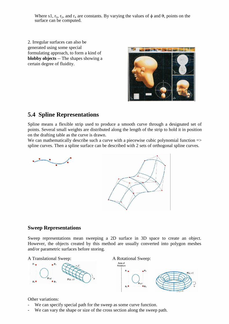
2. Irregular surfaces can also be

generated using some special

formulating approach, to form a kind of

blobby objects -- The shapes showing a

certain degree of fluidity.

5.4 Spline Representations Spline means a flexible strip used to produce a smooth curve through a designated set of

points. Several small weights are distributed along the length of the strip to hold it in position

on the drafting table as the curve is drawn. We can mathematically describe such a curve with a piecewise cubic polynomial function =>

spline curves. Then a spline surface can be described with 2 sets of orthogonal spline curves.

Sweep Representations Sweep representations mean sweeping a 2D surface in 3D space to create an object.

However, the objects created by this method are usually converted into polygon meshes

and/or parametric surfaces before storing. A Translational Sweep: A Rotational Sweep: Other variations: - We can specify special path for the sweep as some curve function. - We can vary the shape or size of the cross section along the sweep path.

- We can also vary the orientation of the cross section relative to the sweep path.

Unit-6

Three Dimensional Transformations:

Methods for geometric transforamtions and object modelling in 3D are extended from 2D

methods by including

the considerations for the z coordinate.

Basic geometric transformations are: Translation, Rotation, Scaling

6.1 Basic Transformations

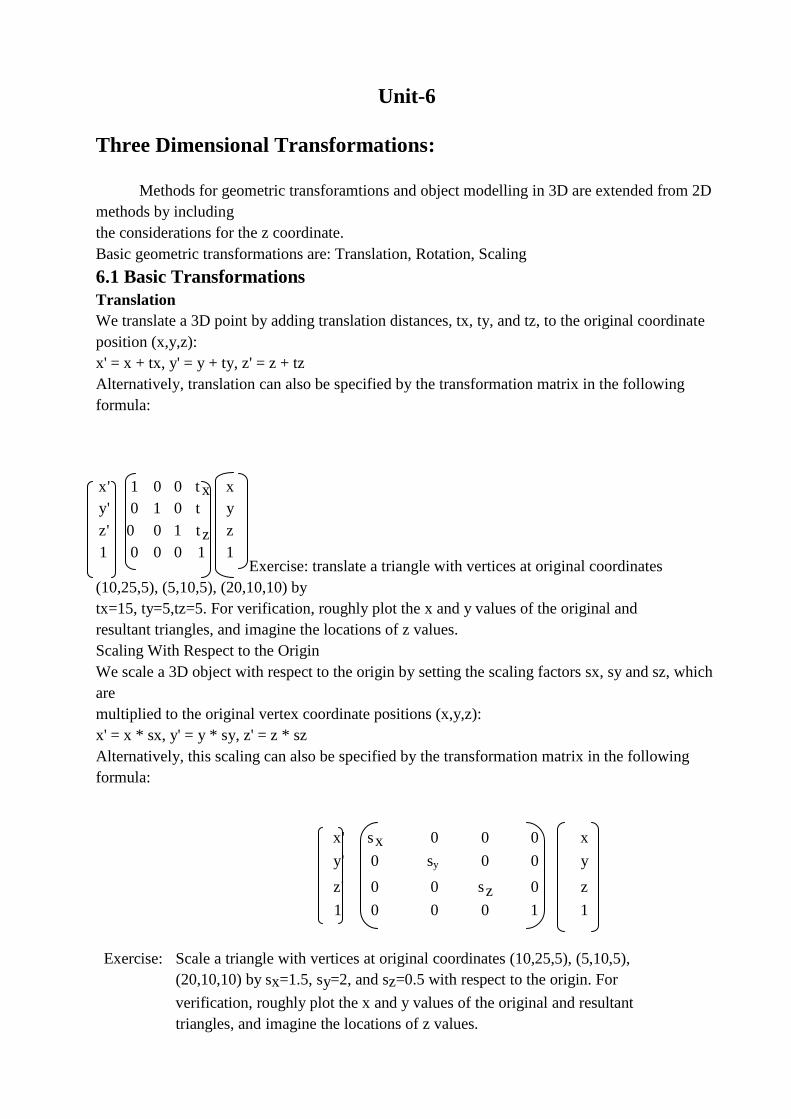
Translation

We translate a 3D point by adding translation distances, tx, ty, and tz, to the original coordinate

position (x,y,z):

x' = x + tx, y' = y + ty, z' = z + tz

Alternatively, translation can also be specified by the transformation matrix in the following

formula:

Exercise: translate a triangle with vertices at original coordinates

(10,25,5), (5,10,5), (20,10,10) by

tx=15, ty=5,tz=5. For verification, roughly plot the x and y values of the original and

resultant triangles, and imagine the locations of z values.

Scaling With Respect to the Origin

We scale a 3D object with respect to the origin by setting the scaling factors sx, sy and sz, which

are

multiplied to the original vertex coordinate positions (x,y,z):

x' = x * sx, y' = y * sy, z' = z * sz

Alternatively, this scaling can also be specified by the transformation matrix in the following

formula:

x' s x 0 0 0 x

y' 0 sy 0 0 y

z' 0 0 s z 0 z

1 0 0 0 1 1

Exercise: Scale a triangle with vertices at original coordinates (10,25,5), (5,10,5),

(20,10,10) by sx=1.5, sy=2, and sz=0.5 with respect to the origin. For

verification, roughly plot the x and y values of the original and resultant

triangles, and imagine the locations of z values.

x' 1 0 0 t x x

y' 0 1 0 t y

z' 0 0 1 t z z

1 0 0 0 1 1

6.2 Scaling with respect to a Selected Fixed Position

Exercise: What are the steps to perform scaling with respect to a selected fixed

position? Check your answer with the text book.

Exercise: Scale a triangle with vertices at original coordinates (10,25,5), (5,10,5),

(20,10,10) by sx=1.5, sy=2, and sz=0.5 with respect to the centre of the triangle.

For verification, roughly plot the x and y values of the original and resultant

triangles, and imagine the locations of z values.

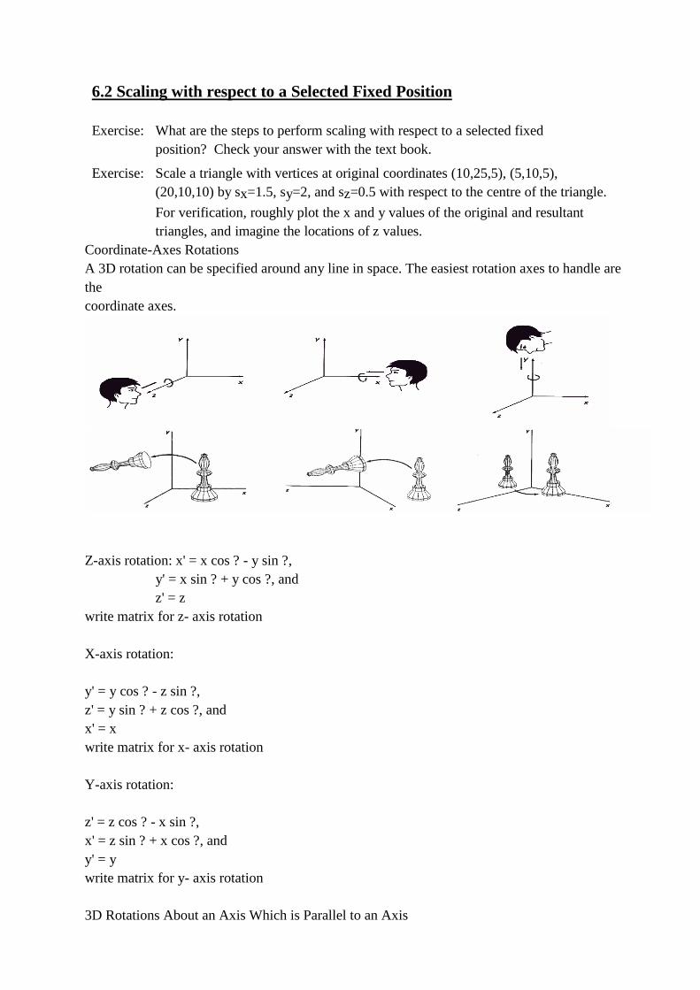
Coordinate-Axes Rotations

A 3D rotation can be specified around any line in space. The easiest rotation axes to handle are

the

coordinate axes.

Z-axis rotation: x' = x cos ? - y sin ?,

y' = x sin ? + y cos ?, and

z' = z

write matrix for z- axis rotation

X-axis rotation:

y' = y cos ? - z sin ?,

z' = y sin ? + z cos ?, and

x' = x

write matrix for x- axis rotation

Y-axis rotation:

z' = z cos ? - x sin ?,

x' = z sin ? + x cos ?, and

y' = y

write matrix for y- axis rotation

3D Rotations About an Axis Which is Parallel to an Axis

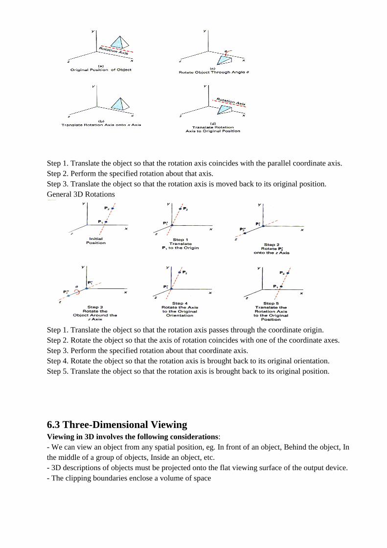
Step 1. Translate the object so that the rotation axis coincides with the parallel coordinate axis.

Step 2. Perform the specified rotation about that axis.

Step 3. Translate the object so that the rotation axis is moved back to its original position.

General 3D Rotations

Step 1. Translate the object so that the rotation axis passes through the coordinate origin.

Step 2. Rotate the object so that the axis of rotation coincides with one of the coordinate axes.

Step 3. Perform the specified rotation about that coordinate axis.

Step 4. Rotate the object so that the rotation axis is brought back to its original orientation.

Step 5. Translate the object so that the rotation axis is brought back to its original position.

6.3 Three-Dimensional Viewing Viewing in 3D involves the following considerations:

- We can view an object from any spatial position, eg. In front of an object, Behind the object, In

the middle of a group of objects, Inside an object, etc.

- 3D descriptions of objects must be projected onto the flat viewing surface of the output device.

- The clipping boundaries enclose a volume of space

6.4 Viewing Pipeline

Modelling

Coordinates

Modelling

Transformations

Explanation

World

Coordinates

Viewing

Coordinates

Projection

Transformation

Projection

Coordinates

Workstation

Transformation

Device

Coordinates

Modelling Transformation and Viewing Transformation can be done by 3D transformations.

The viewing-coordinate system is used in graphics packages as a reference for specifying the

observer viewing position and the position of the projection plane. Projection operations convert

the viewing-coordinate description (3D) to coordinate positions on the projection plane (2D).

(Usually combined with clipping, visual-surface identification, and surface-

rendering)Workstation transformation maps the coordinate positions on the

Viewing

Transformation

projection plane to the output device

6.5 Viewing Transformation Conversion of objection descriptions from world to viewing coordinates is equivalent to a

transformation that superimposes the viewing reference frame onto the world frame using the

basic

geometric translate-rotate operations:

1. Translate the view reference point to the origin of the world-coordinate system.

2. Apply rotations to align the xv, yv, and zv axes (viewing coordinate system) with the world

xw, yw,

zw axes, respectively.

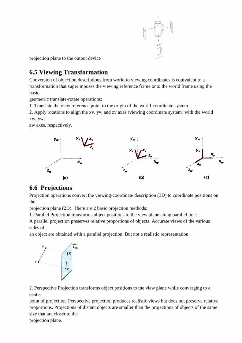
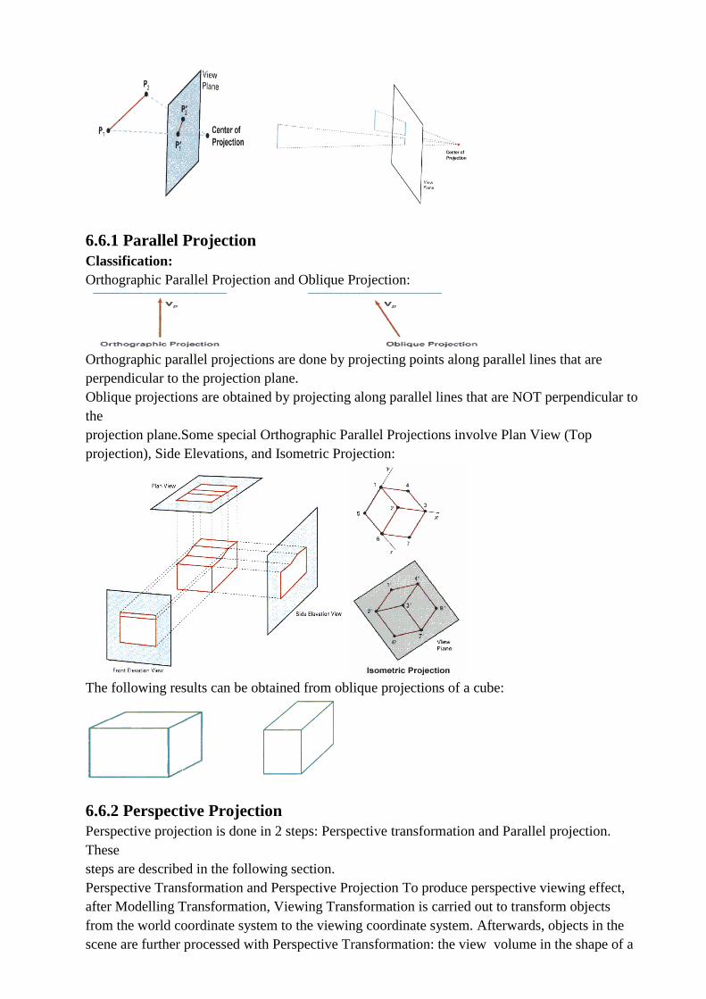
6.6 Projections Projection operations convert the viewing-coordinate description (3D) to coordinate positions on

the

projection plane (2D). There are 2 basic projection methods:

1. Parallel Projection transforms object positions to the view plane along parallel lines.

A parallel projection preserves relative proportions of objects. Accurate views of the various

sides of

an object are obtained with a parallel projection. But not a realistic representation

2. Perspective Projection transforms object positions to the view plane while converging to a

center

point of projection. Perspective projection produces realistic views but does not preserve relative

proportions. Projections of distant objects are smaller than the projections of objects of the same

size that are closer to the

projection plane.

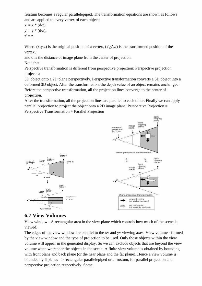
6.6.1 Parallel Projection

Classification:

Orthographic Parallel Projection and Oblique Projection:

Orthographic parallel projections are done by projecting points along parallel lines that are

perpendicular to the projection plane.

Oblique projections are obtained by projecting along parallel lines that are NOT perpendicular to

the

projection plane.Some special Orthographic Parallel Projections involve Plan View (Top

projection), Side Elevations, and Isometric Projection:

The following results can be obtained from oblique projections of a cube:

6.6.2 Perspective Projection

Perspective projection is done in 2 steps: Perspective transformation and Parallel projection.

These

steps are described in the following section.

Perspective Transformation and Perspective Projection To produce perspective viewing effect,

after Modelling Transformation, Viewing Transformation is carried out to transform objects

from the world coordinate system to the viewing coordinate system. Afterwards, objects in the

scene are further processed with Perspective Transformation: the view volume in the shape of a

frustum becomes a regular parallelepiped. The transformation equations are shown as follows

and are applied to every vertex of each object:

x' = x * (d/z),

y' = y * (d/z),

z' = z

Where (x,y,z) is the original position of a vertex, (x',y',z') is the transformed position of the

vertex,

and d is the distance of image plane from the center of projection.

Note that:

Perspective transformation is different from perspective projection: Perspective projection

projects a

3D object onto a 2D plane perspectively. Perspective transformation converts a 3D object into a

deformed 3D object. After the transformation, the depth value of an object remains unchanged.

Before the perspective transformation, all the projection lines converge to the center of

projection.

After the transformation, all the projection lines are parallel to each other. Finally we can apply

parallel projection to project the object onto a 2D image plane. Perspective Projection =

Perspective Transformation + Parallel Projection

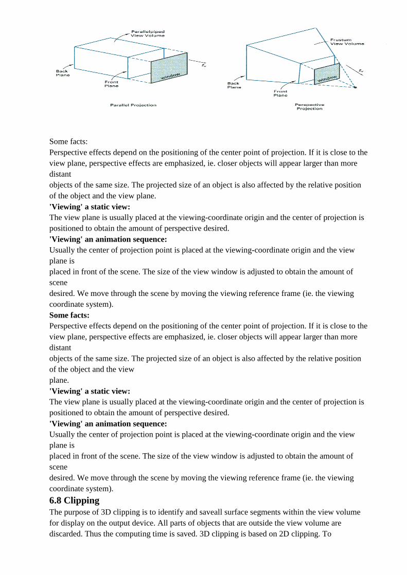
6.7 View Volumes View window - A rectangular area in the view plane which controls how much of the scene is

viewed.

The edges of the view window are parallel to the xv and yv viewing axes. View volume - formed

by the view window and the type of projection to be used. Only those objects within the view

volume will appear in the generated display. So we can exclude objects that are beyond the view

volume when we render the objects in the scene. A finite view volume is obtained by bounding

with front plane and back plane (or the near plane and the far plane). Hence a view volume is

bounded by 6 planes => rectangular parallelepiped or a frustum, for parallel projection and

perspective projection respectively. Some

Some facts:

Perspective effects depend on the positioning of the center point of projection. If it is close to the

view plane, perspective effects are emphasized, ie. closer objects will appear larger than more

distant

objects of the same size. The projected size of an object is also affected by the relative position

of the object and the view plane.

'Viewing' a static view:

The view plane is usually placed at the viewing-coordinate origin and the center of projection is

positioned to obtain the amount of perspective desired.

'Viewing' an animation sequence:

Usually the center of projection point is placed at the viewing-coordinate origin and the view

plane is

placed in front of the scene. The size of the view window is adjusted to obtain the amount of

scene

desired. We move through the scene by moving the viewing reference frame (ie. the viewing

coordinate system).

Some facts:

Perspective effects depend on the positioning of the center point of projection. If it is close to the

view plane, perspective effects are emphasized, ie. closer objects will appear larger than more

distant

objects of the same size. The projected size of an object is also affected by the relative position

of the object and the view

plane.

'Viewing' a static view:

The view plane is usually placed at the viewing-coordinate origin and the center of projection is

positioned to obtain the amount of perspective desired.

'Viewing' an animation sequence:

Usually the center of projection point is placed at the viewing-coordinate origin and the view

plane is

placed in front of the scene. The size of the view window is adjusted to obtain the amount of

scene

desired. We move through the scene by moving the viewing reference frame (ie. the viewing

coordinate system).

6.8 Clipping

The purpose of 3D clipping is to identify and saveall surface segments within the view volume

for display on the output device. All parts of objects that are outside the view volume are

discarded. Thus the computing time is saved. 3D clipping is based on 2D clipping. To

understand the basic concept we consider the

following algorithm:

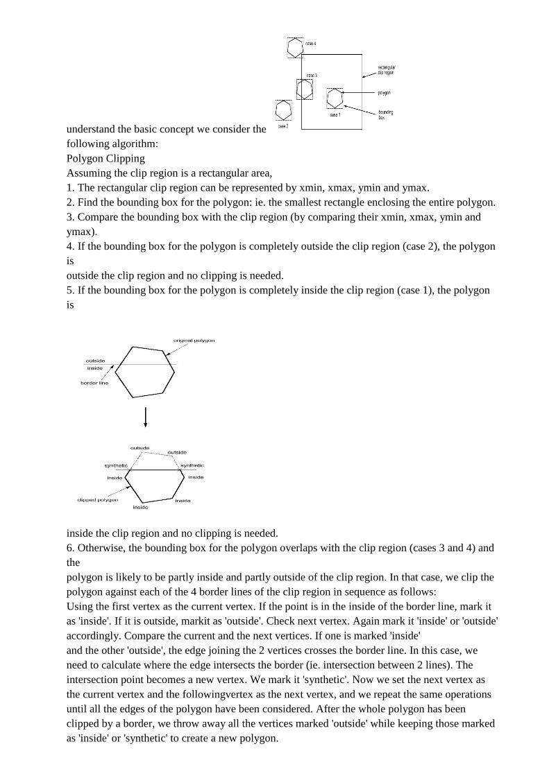
Polygon Clipping

Assuming the clip region is a rectangular area,

1. The rectangular clip region can be represented by xmin, xmax, ymin and ymax.

2. Find the bounding box for the polygon: ie. the smallest rectangle enclosing the entire polygon.

3. Compare the bounding box with the clip region (by comparing their xmin, xmax, ymin and

ymax).

4. If the bounding box for the polygon is completely outside the clip region (case 2), the polygon

is

outside the clip region and no clipping is needed.

5. If the bounding box for the polygon is completely inside the clip region (case 1), the polygon

is

inside the clip region and no clipping is needed.

6. Otherwise, the bounding box for the polygon overlaps with the clip region (cases 3 and 4) and

the

polygon is likely to be partly inside and partly outside of the clip region. In that case, we clip the

polygon against each of the 4 border lines of the clip region in sequence as follows:

Using the first vertex as the current vertex. If the point is in the inside of the border line, mark it

as 'inside'. If it is outside, markit as 'outside'. Check next vertex. Again mark it 'inside' or 'outside'

accordingly. Compare the current and the next vertices. If one is marked 'inside'

and the other 'outside', the edge joining the 2 vertices crosses the border line. In this case, we

need to calculate where the edge intersects the border (ie. intersection between 2 lines). The

intersection point becomes a new vertex. We mark it 'synthetic'. Now we set the next vertex as

the current vertex and the followingvertex as the next vertex, and we repeat the same operations

until all the edges of the polygon have been considered. After the whole polygon has been

clipped by a border, we throw away all the vertices marked 'outside' while keeping those marked

as 'inside' or 'synthetic' to create a new polygon.

We repeat the clipping process with the new polygon against the next border line of the clip

region.

7. This clipping operation results in a polygon which is totally inside the clip region.

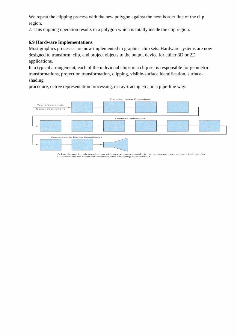
6.9 Hardware Implementations

Most graphics processes are now implemented in graphics chip sets. Hardware systems are now

designed to transform, clip, and project objects to the output device for either 3D or 2D

applications.

In a typical arrangement, each of the individual chips in a chip set is responsible for geometric

transformations, projection transformation, clipping, visible-surface identification, surface-

shading

procedure, octree representation processing, or ray-tracing etc., in a pipe-line way.

Unit-7

Visible-Surface Detection Methods

More information about Modelling and Perspective Viewing:

Before going to visible surface detection, we first review and discuss the followings:

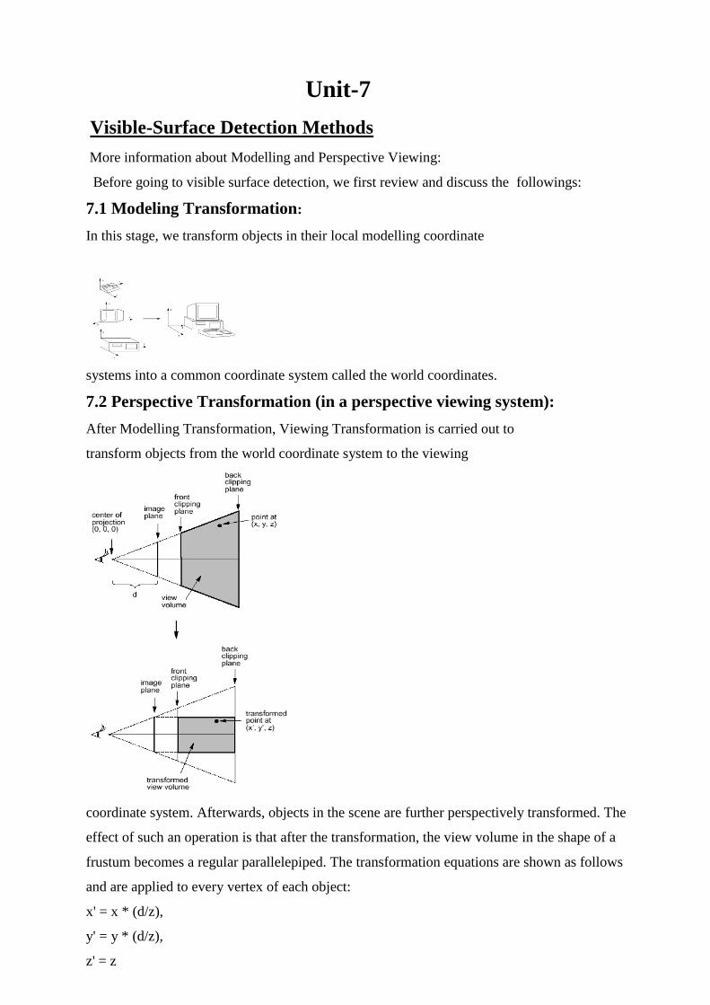
7.1 Modeling Transformation:

In this stage, we transform objects in their local modelling coordinate

systems into a common coordinate system called the world coordinates.

7.2 Perspective Transformation (in a perspective viewing system):

After Modelling Transformation, Viewing Transformation is carried out to

transform objects from the world coordinate system to the viewing

coordinate system. Afterwards, objects in the scene are further perspectively transformed. The

effect of such an operation is that after the transformation, the view volume in the shape of a

frustum becomes a regular parallelepiped. The transformation equations are shown as follows

and are applied to every vertex of each object:

x' = x * (d/z),

y' = y * (d/z),

z' = z

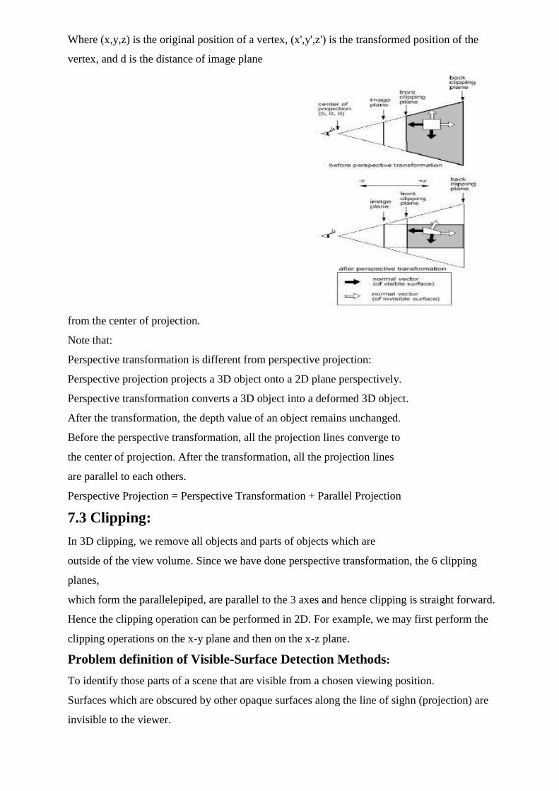
Where (x,y,z) is the original position of a vertex, (x',y',z') is the transformed position of the

vertex, and d is the distance of image plane

from the center of projection.

Note that:

Perspective transformation is different from perspective projection:

Perspective projection projects a 3D object onto a 2D plane perspectively.

Perspective transformation converts a 3D object into a deformed 3D object.

After the transformation, the depth value of an object remains unchanged.

Before the perspective transformation, all the projection lines converge to

the center of projection. After the transformation, all the projection lines

are parallel to each others.

Perspective Projection = Perspective Transformation + Parallel Projection

7.3 Clipping:

In 3D clipping, we remove all objects and parts of objects which are

outside of the view volume. Since we have done perspective transformation, the 6 clipping

planes,

which form the parallelepiped, are parallel to the 3 axes and hence clipping is straight forward.

Hence the clipping operation can be performed in 2D. For example, we may first perform the

clipping operations on the x-y plane and then on the x-z plane.

Problem definition of Visible-Surface Detection Methods:

To identify those parts of a scene that are visible from a chosen viewing position.

Surfaces which are obscured by other opaque surfaces along the line of sighn (projection) are

invisible to the viewer.

Characteristics of approaches:

- Require large memory size?

- Require long processing time?

- Applicable to which types of objects?

Considerations:

- Complexity of the scene

- Type of objects in the scene

- Available equipment

- Static or animated?

Classification of Visible-Surface Detection Algorithms:

7.4 Object-space Methods

Compare objects and parts of objects to each other within the scene definition to determine

which

surfaces, as a whole, we should label as visible:

For each object in the scene do

Begin

1. Determine those part of the object whose view is unobstructed by other parts of it or

any other object with respect to the viewing specification.

2. Draw those parts in the object color.

End

- Compare each object with all other objects to determine the visibility of the object parts.

- If there are n objects in the scene, complexity = O(n2)

- Calculations are performed at the resolution in which the objects are defined (only limited by

the

computation hardware).

- Process is unrelated to display resolution or the individual pixel in the image and the result of

the

process is applicable to different display resolutions.

- Display is more accurate but computationally more expensive as compared to image space

methods because step 1 is typically more complex, eg. Due to the possibility of intersection

between surfaces.

- Suitable for scene with small number of objects and objects with simple relationship with each

other.

7.5 Image-space Methods (Mostly used)

Visibility is determined point by point at each pixel position on the projection plane.

For each pixel in the image do

Begin

1. Determine the object closest to the viewer that is pierced by the projector through the

pixel

2. Draw the pixel in the object colour.

End

- For each pixel, examine all n objects to determine the one closest to the viewer.

- If there are p pixels in the image, complexity depends on n and p ( O(np) ).

- Accuarcy of the calculation is bounded by the display resolution.

- A change of display resolution requires re-calculation

Application of Coherence in Visible Surface Detection Methods:

- Making use of the results calculated for one part of the scene or image for other nearby parts.

- Coherence is the result of local similarity

- As objects have continuous spatial extent, object properties vary smoothly within a small local

region in the scene. Calculations can then be made incremental.

Types of coherence:

1. Object Coherence:

Visibility of an object can often be decided by examining a circumscribing solid (which may be

of

simple form, eg. A sphere or a polyhedron.)

2. Face Coherence:

Surface properties computed for one part of a face can be applied to adjacent parts after small

incremental modification. (eg. If the face is small, we sometimes can assume if one part of the

face is

invisible to the viewer, the entire face is also invisible).

3. Edge Coherence:

The Visibility of an edge changes only when it crosses another edge, so if one segment of an

nonintersecting edge is visible, the entire edge is also visible.

4. Scan line Coherence:

Line or surface segments visible in one scan line are also likely to be visible in adjacent scan

lines.

Consequently, the image of a scan line is similar to the image of adjacent scan lines.

5. Area and Span Coherence:

A group of adjacent pixels in an image is often covered by the same visible object. This

coherence is

based on the assumption that a small enough region of pixels will most likely lie within a single

polygon. This reduces computation effort in searching for those polygons which contain a given

screen area (region of pixels) as in some subdivision algorithms.

6. Depth Coherence:

The depths of adjacent parts of the same surface are similar.

7. Frame Coherence:

Pictures of the same scene at successive points in time are likely to be similar, despite small

changes

in objects and viewpoint, except near the edges of moving objects. Most visible surface detection

methods make use of one or more of these coherence properties of a scene. To take advantage of

regularities in a scene, eg. Constant relationships often can be established between objects and

surfaces in a scene.

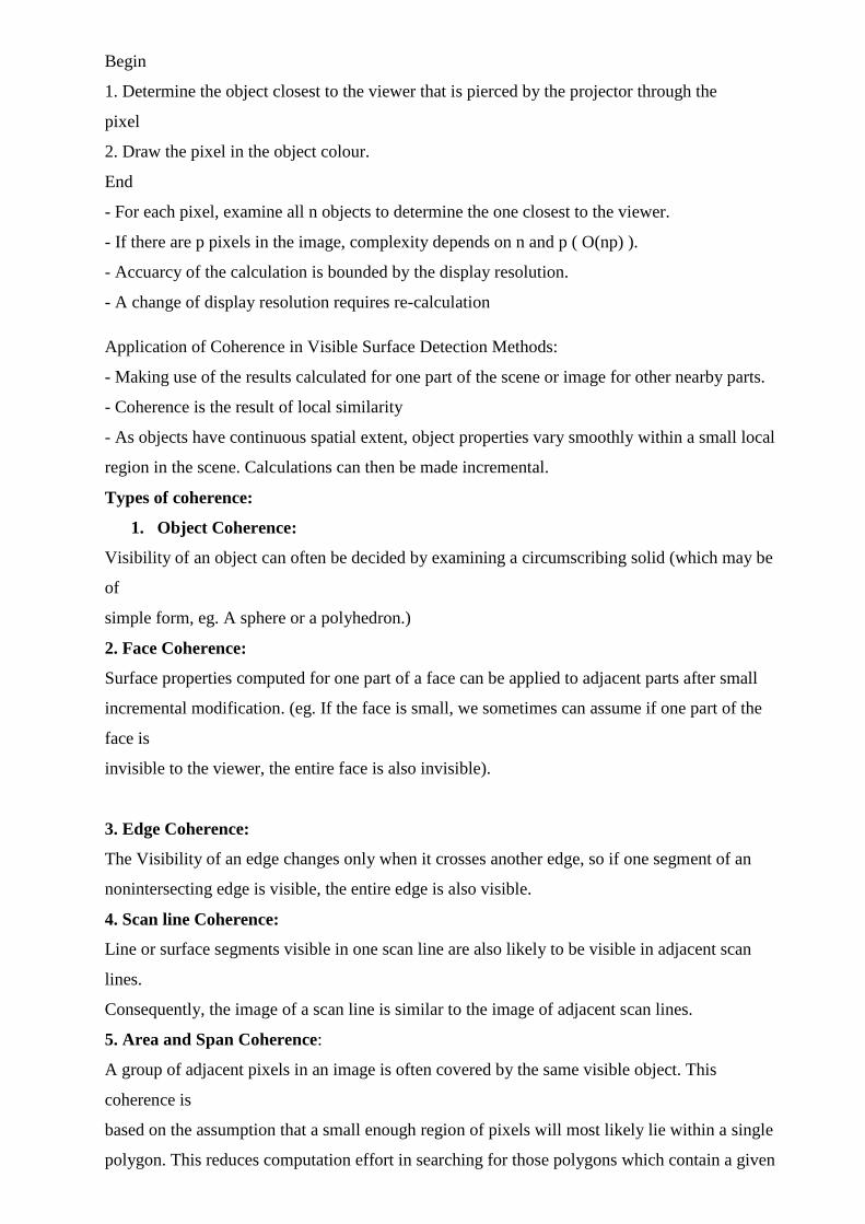
7.6 Back-Face Detection

In a solid object, there are surfaces which are facing the viewer (front faces) and there are

surfaces

which are opposite to the viewer (back faces). These back faces contribute to approximately half

of the total number of surfaces. Since we cannot see these surfaces anyway, to save processing

time, we can remove them before the clipping process with a simple test. Each surface has a

normal vector. If this vector is pointing in the direction of the center of projection, it is a front

face and can be seen by the viewer. If it is pointing away from the center of projection, it is a

back face and cannot be seen by the viewer. The test is very simple, if the z component of the

normal vector is positive, then, it is a back face. If the z component of the vector is negative, it is

a front face. Note that this technique only caters well for non overlapping convex polyhedral.

For other cases where there are concave polyhedra or

overlapping objects, we still need to apply other methods to further determine where the

obscured faces are partially or completely

hidden by other objects (eg.Using Depth-Buffer Method or Depth-sort Method).

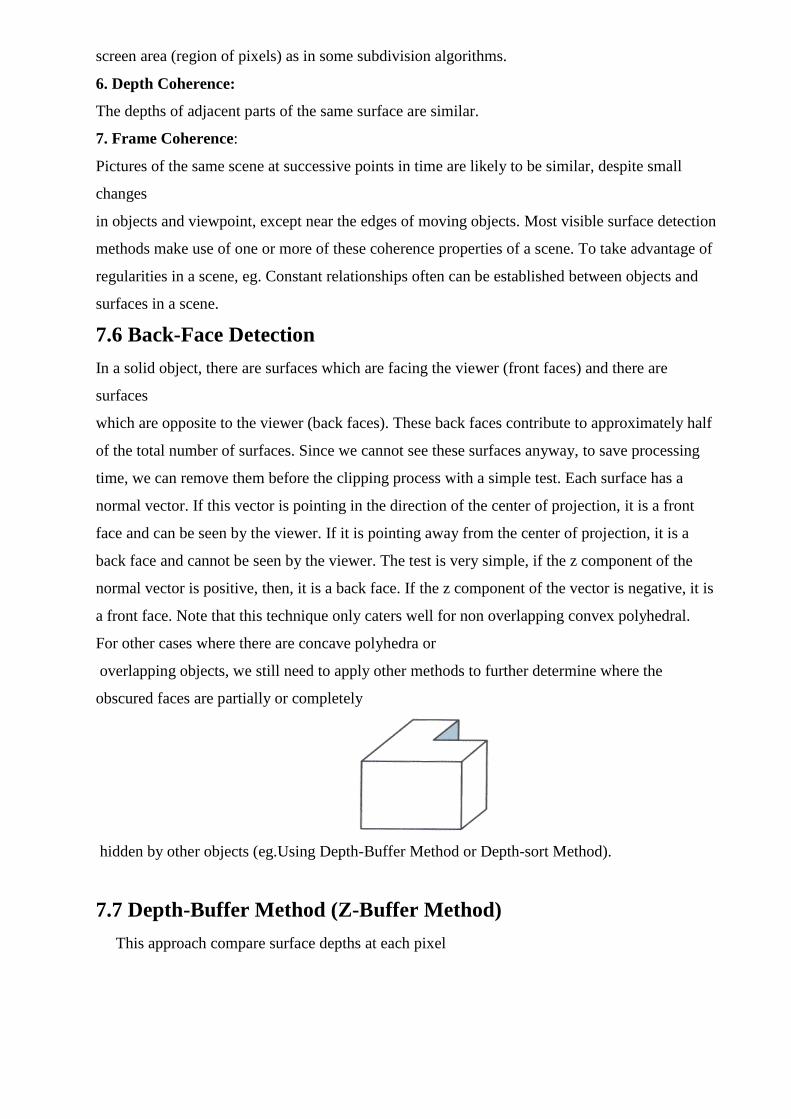
7.7 Depth-Buffer Method (Z-Buffer Method)

This approach compare surface depths at each pixel

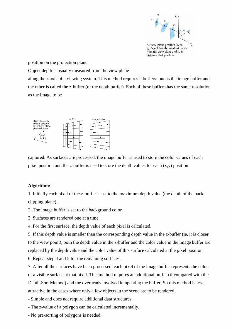
position on the projection plane.

Object depth is usually measured from the view plane

along the z axis of a viewing system. This method requires 2 buffers: one is the image buffer and

the other is called the z-buffer (or the depth buffer). Each of these buffers has the same resolution

as the image to be

captured. As surfaces are processed, the image buffer is used to store the color values of each

pixel position and the z-buffer is used to store the depth values for each (x,y) position.

Algorithm:

1. Initially each pixel of the z-buffer is set to the maximum depth value (the depth of the back

clipping plane).

2. The image buffer is set to the background color.

3. Surfaces are rendered one at a time.

4. For the first surface, the depth value of each pixel is calculated.

5. If this depth value is smaller than the corresponding depth value in the z-buffer (ie. it is closer

to the view point), both the depth value in the z-buffer and the color value in the image buffer are

replaced by the depth value and the color value of this surface calculated at the pixel position.

6. Repeat step 4 and 5 for the remaining surfaces.

7. After all the surfaces have been processed, each pixel of the image buffer represents the color

of a visible surface at that pixel. This method requires an additional buffer (if compared with the

Depth-Sort Method) and the overheads involved in updating the buffer. So this method is less

attractive in the cases where only a few objects in the scene are to be rendered.

- Simple and does not require additional data structures.

- The z-value of a polygon can be calculated incrementally.

- No pre-sorting of polygons is needed.

- No object-object comparison is required.

- Can be applied to non-polygonal objects.

- Hardware implementations of the algorithm are available in some graphics workstation.

- For large images, the algorithm could be applied to, eg., the 4 quadrants of the image

separately, so as to reduce the requirement of a large additional buffer

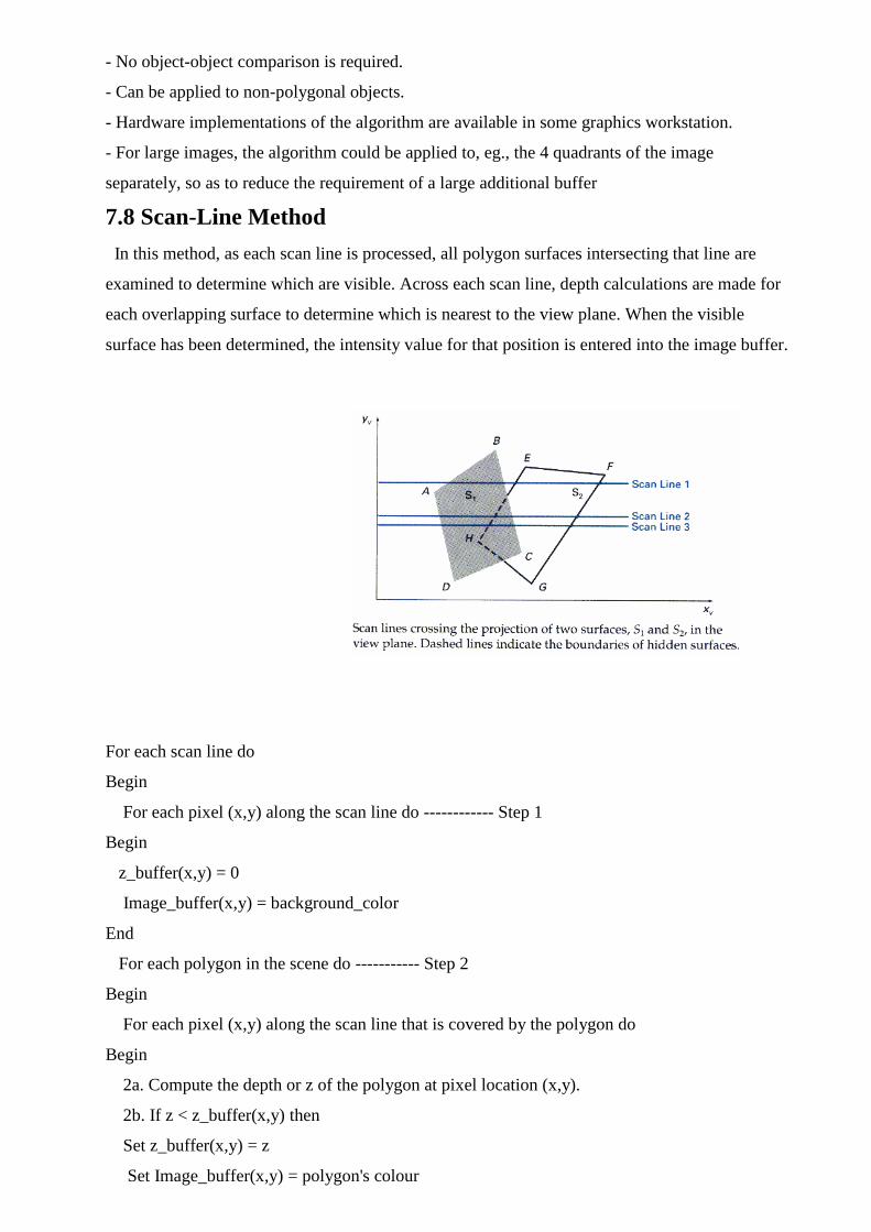
7.8 Scan-Line Method

In this method, as each scan line is processed, all polygon surfaces intersecting that line are

examined to determine which are visible. Across each scan line, depth calculations are made for

each overlapping surface to determine which is nearest to the view plane. When the visible

surface has been determined, the intensity value for that position is entered into the image buffer.

For each scan line do

Begin

For each pixel (x,y) along the scan line do ------------ Step 1

Begin

z_buffer(x,y) = 0

Image_buffer(x,y) = background_color

End

For each polygon in the scene do ----------- Step 2

Begin

For each pixel (x,y) along the scan line that is covered by the polygon do

Begin

2a. Compute the depth or z of the polygon at pixel location (x,y).

2b. If z < z_buffer(x,y) then

Set z_buffer(x,y) = z

Set Image_buffer(x,y) = polygon's colour

End

End

End

- Step 2 is not efficient because not all polygons necessarily intersect with the scan line.

- Depth calculation in 2a is not needed if only 1 polygon in the scene is mapped onto a segment

of

the scan line.

- To speed up the process:

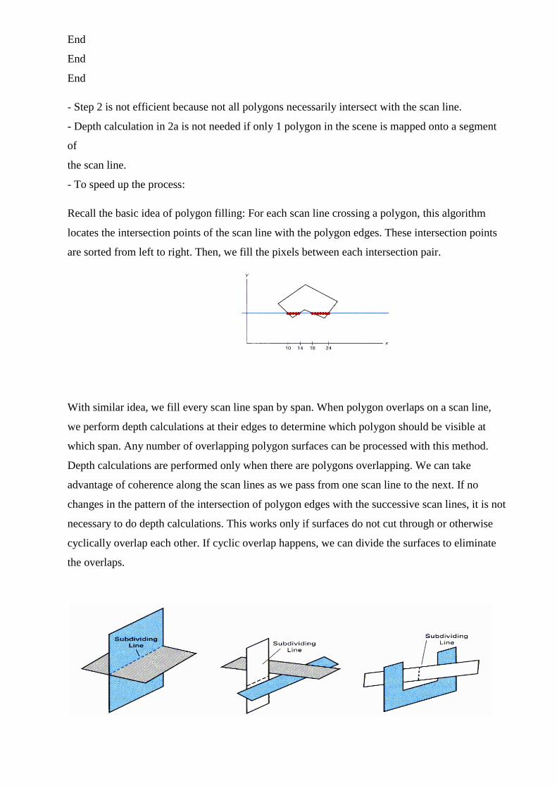
Recall the basic idea of polygon filling: For each scan line crossing a polygon, this algorithm

locates the intersection points of the scan line with the polygon edges. These intersection points

are sorted from left to right. Then, we fill the pixels between each intersection pair.

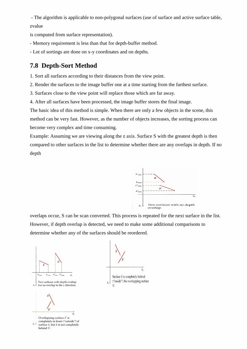
With similar idea, we fill every scan line span by span. When polygon overlaps on a scan line,

we perform depth calculations at their edges to determine which polygon should be visible at

which span. Any number of overlapping polygon surfaces can be processed with this method.

Depth calculations are performed only when there are polygons overlapping. We can take

advantage of coherence along the scan lines as we pass from one scan line to the next. If no

changes in the pattern of the intersection of polygon edges with the successive scan lines, it is not

necessary to do depth calculations. This works only if surfaces do not cut through or otherwise

cyclically overlap each other. If cyclic overlap happens, we can divide the surfaces to eliminate

the overlaps.

- The algorithm is applicable to non-polygonal surfaces (use of surface and active surface table,

zvalue

is computed from surface representation).

- Memory requirement is less than that for depth-buffer method.

- Lot of sortings are done on x-y coordinates and on depths.

7.8 Depth-Sort Method

1. Sort all surfaces according to their distances from the view point.

2. Render the surfaces to the image buffer one at a time starting from the farthest surface.

3. Surfaces close to the view point will replace those which are far away.

4. After all surfaces have been processed, the image buffer stores the final image.

The basic idea of this method is simple. When there are only a few objects in the scene, this

method can be very fast. However, as the number of objects increases, the sorting process can

become very complex and time consuming.

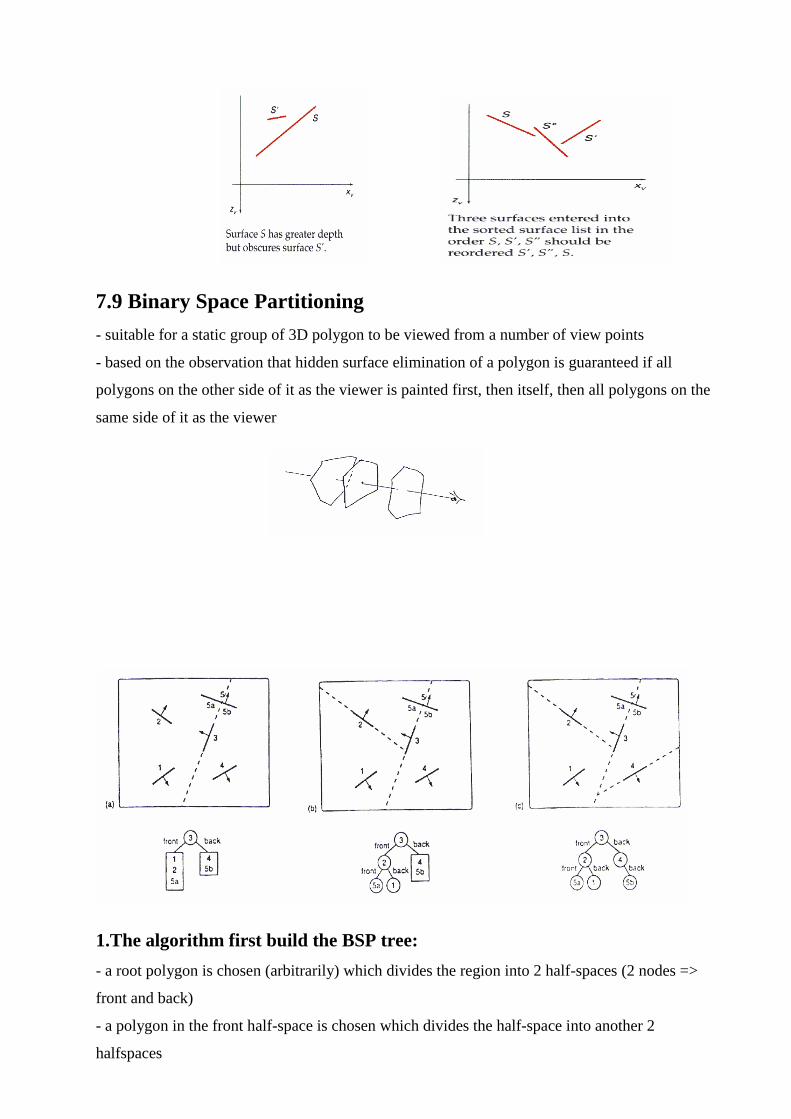
Example: Assuming we are viewing along the z axis. Surface S with the greatest depth is then

compared to other surfaces in the list to determine whether there are any overlaps in depth. If no

depth

overlaps occur, S can be scan converted. This process is repeated for the next surface in the list.

However, if depth overlap is detected, we need to make some additional comparisons to

determine whether any of the surfaces should be reordered.

7.9 Binary Space Partitioning

- suitable for a static group of 3D polygon to be viewed from a number of view points

- based on the observation that hidden surface elimination of a polygon is guaranteed if all

polygons on the other side of it as the viewer is painted first, then itself, then all polygons on the

same side of it as the viewer

1.The algorithm first build the BSP tree:

- a root polygon is chosen (arbitrarily) which divides the region into 2 half-spaces (2 nodes =>

front and back)

- a polygon in the front half-space is chosen which divides the half-space into another 2

halfspaces

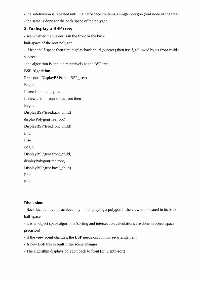
- the subdivision is repeated until the half-space contains a single polygon (leaf node of the tree)

- the same is done for the back space of the polygon.

2.To display a BSP tree:

- see whether the viewer is in the front or the back

half-space of the root polygon.

- if front half-space then first display back child (subtree) then itself, followed by its front child /

subtree

- the algorithm is applied recursively to the BSP tree.

BSP Algorithm

Procedure DisplayBSP(tree: BSP_tree)

Begin

If tree is not empty then

If viewer is in front of the root then

Begin

DisplayBSP(tree.back_child)

displayPolygon(tree.root)

DisplayBSP(tree.front_child)

End

Else

Begin

DisplayBSP(tree.front_child)

displayPolygon(tree.root)

DisplayBSP(tree.back_child)

End

End

Discussion:

- Back face removal is achieved by not displaying a polygon if the viewer is located in its back

half-space

- It is an object space algorithm (sorting and intersection calculations are done in object space

precision)

- If the view point changes, the BSP needs only minor re-arrangement.

- A new BSP tree is built if the scene changes

- The algorithm displays polygon back to front (cf. Depth-sort)

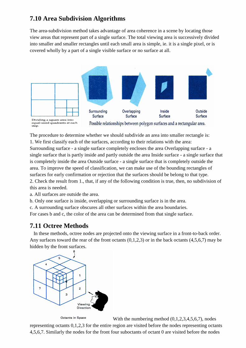
7.10 Area Subdivision Algorithms

The area-subdivision method takes advantage of area coherence in a scene by locating those

view areas that represent part of a single surface. The total viewing area is successively divided

into smaller and smaller rectangles until each small area is simple, ie. it is a single pixel, or is

covered wholly by a part of a single visible surface or no surface at all.

The procedure to determine whether we should subdivide an area into smaller rectangle is:

1. We first classify each of the surfaces, according to their relations with the area:

Surrounding surface - a single surface completely encloses the area Overlapping surface - a

single surface that is partly inside and partly outside the area Inside surface - a single surface that

is completely inside the area Outside surface - a single surface that is completely outside the

area. To improve the speed of classification, we can make use of the bounding rectangles of

surfaces for early confirmation or rejection that the surfaces should be belong to that type.

2. Check the result from 1., that, if any of the following condition is true, then, no subdivision of

this area is needed.

a. All surfaces are outside the area.

b. Only one surface is inside, overlapping or surrounding surface is in the area.

c. A surrounding surface obscures all other surfaces within the area boundaries.

For cases b and c, the color of the area can be determined from that single surface.

7.11 Octree Methods In these methods, octree nodes are projected onto the viewing surface in a front-to-back order.

Any surfaces toward the rear of the front octants (0,1,2,3) or in the back octants (4,5,6,7) may be

hidden by the front surfaces.

With the numbering method (0,1,2,3,4,5,6,7), nodes

representing octants 0,1,2,3 for the entire region are visited before the nodes representing octants

4,5,6,7. Similarly the nodes for the front four suboctants of octant 0 are visited before the nodes

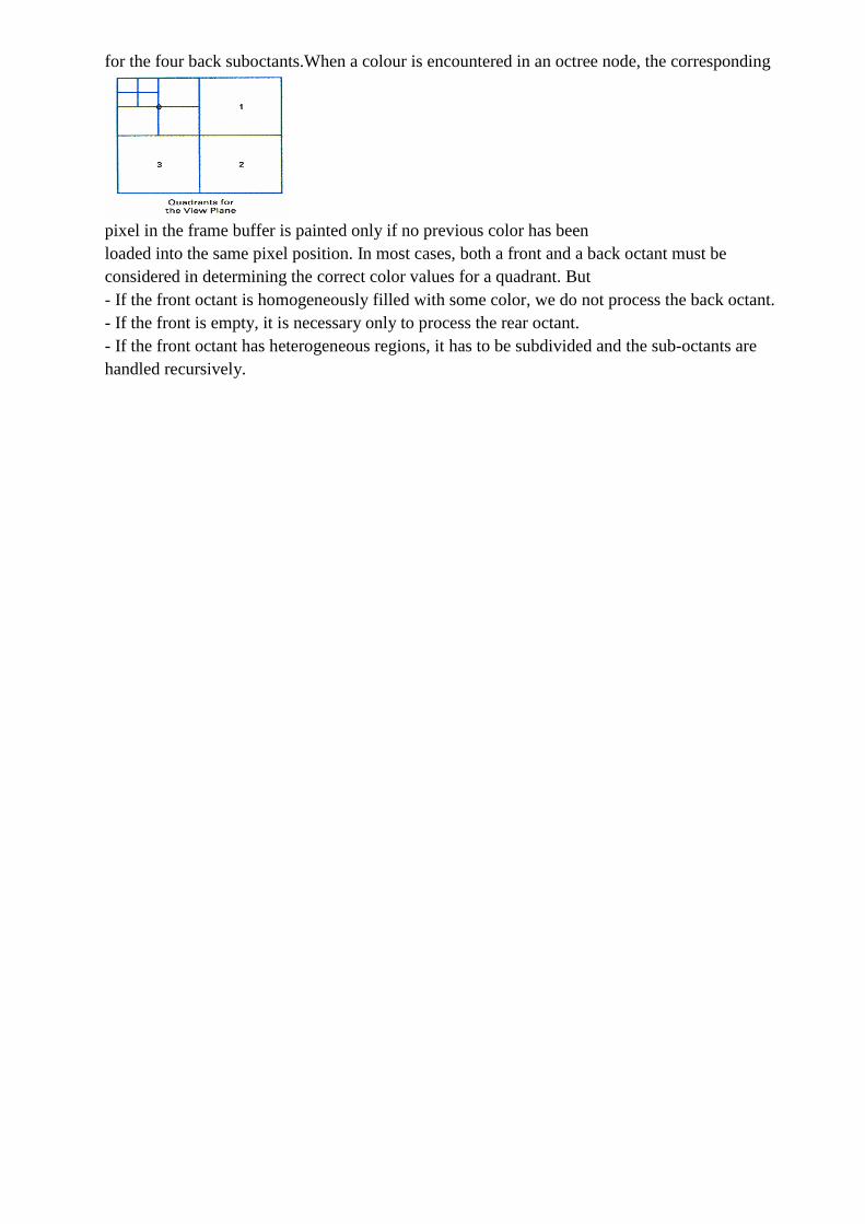
for the four back suboctants.When a colour is encountered in an octree node, the corresponding

pixel in the frame buffer is painted only if no previous color has been

loaded into the same pixel position. In most cases, both a front and a back octant must be

considered in determining the correct color values for a quadrant. But

- If the front octant is homogeneously filled with some color, we do not process the back octant.

- If the front is empty, it is necessary only to process the rear octant.

- If the front octant has heterogeneous regions, it has to be subdivided and the sub-octants are

handled recursively.

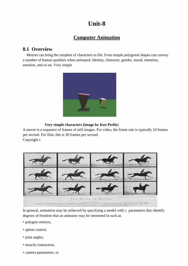
Unit-8

Computer Animation

8.1 Overview Motion can bring the simplest of characters to life. Even simple polygonal shapes can convey

a number of human qualities when animated: identity, character, gender, mood, intention,

emotion, and so on. Very simple

Very simple characters (image by Ken Perlin)

A movie is a sequence of frames of still images. For video, the frame rate is typically 24 frames

per second. For film, this is 30 frames per second.

Copyright c

In general, animation may be achieved by specifying a model with n parameters that identify

degrees of freedom that an animator may be interested in such as

• polygon vertices,

• spline control,

• joint angles,

• muscle contraction,

• camera parameters, or

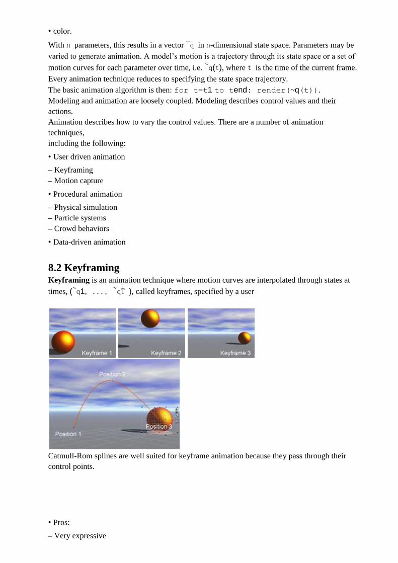
• color.

With n parameters, this results in a vector ~q in n-dimensional state space. Parameters may be

varied to generate animation. A model’s motion is a trajectory through its state space or a set of

motion curves for each parameter over time, i.e. ~q(t), where t is the time of the current frame.

Every animation technique reduces to specifying the state space trajectory.

The basic animation algorithm is then: for t=t1 to tend: render(~q(t)).

Modeling and animation are loosely coupled. Modeling describes control values and their

actions.

Animation describes how to vary the control values. There are a number of animation

techniques,

including the following:

• User driven animation

– Keyframing

– Motion capture

• Procedural animation

– Physical simulation

– Particle systems

– Crowd behaviors

• Data-driven animation

8.2 Keyframing Keyframing is an animation technique where motion curves are interpolated through states at

times, (~q1, ..., ~qT ), called keyframes, specified by a user

Catmull-Rom splines are well suited for keyframe animation because they pass through their

control points.

• Pros:

– Very expressive

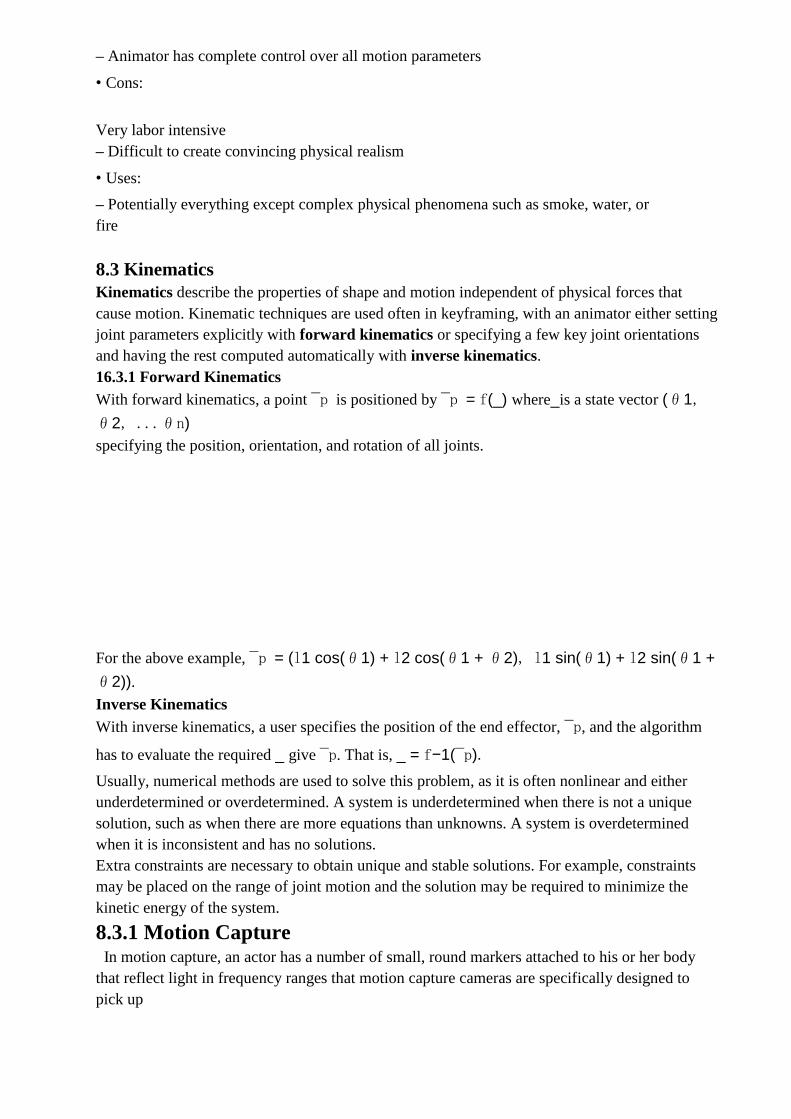
– Animator has complete control over all motion parameters

• Cons:

Very labor intensive

– Difficult to create convincing physical realism

• Uses:

– Potentially everything except complex physical phenomena such as smoke, water, or

fire

8.3 Kinematics

Kinematics describe the properties of shape and motion independent of physical forces that

cause motion. Kinematic techniques are used often in keyframing, with an animator either setting

joint parameters explicitly with forward kinematics or specifying a few key joint orientations

and having the rest computed automatically with inverse kinematics.

16.3.1 Forward Kinematics

With forward kinematics, a point ¯p is positioned by ¯p = f(_) where_is a state vector (θ1,

θ2, ...θn)

specifying the position, orientation, and rotation of all joints.

For the above example, ¯p = (l1 cos(θ1) + l2 cos(θ1 + θ2), l1 sin(θ1) + l2 sin(θ1 +

θ2)).

Inverse Kinematics

With inverse kinematics, a user specifies the position of the end effector, ¯p, and the algorithm

has to evaluate the required _ give ¯p. That is, _ = f−1(¯p).

Usually, numerical methods are used to solve this problem, as it is often nonlinear and either

underdetermined or overdetermined. A system is underdetermined when there is not a unique

solution, such as when there are more equations than unknowns. A system is overdetermined

when it is inconsistent and has no solutions.

Extra constraints are necessary to obtain unique and stable solutions. For example, constraints

may be placed on the range of joint motion and the solution may be required to minimize the

kinetic energy of the system.

8.3.1 Motion Capture In motion capture, an actor has a number of small, round markers attached to his or her body

that reflect light in frequency ranges that motion capture cameras are specifically designed to

pick up

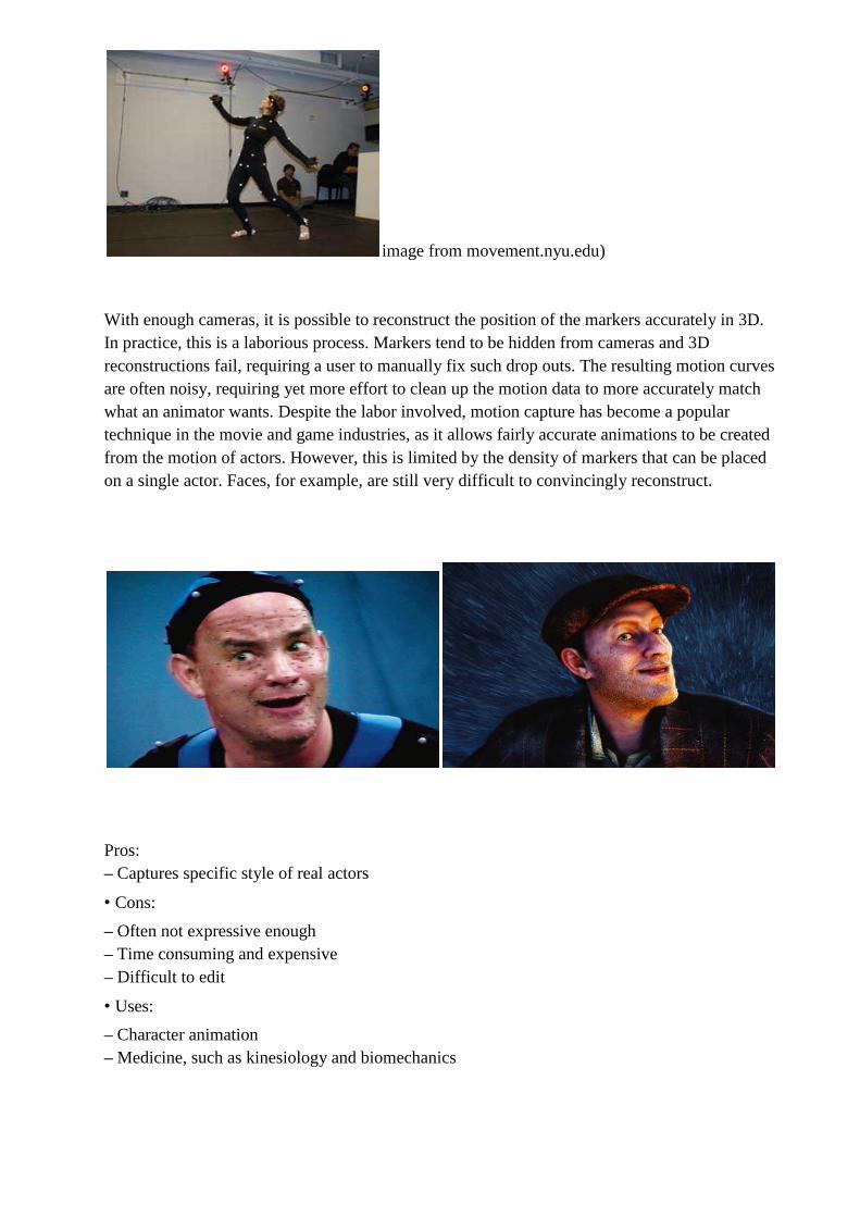
image from movement.nyu.edu)

With enough cameras, it is possible to reconstruct the position of the markers accurately in 3D.

In practice, this is a laborious process. Markers tend to be hidden from cameras and 3D

reconstructions fail, requiring a user to manually fix such drop outs. The resulting motion curves

are often noisy, requiring yet more effort to clean up the motion data to more accurately match

what an animator wants. Despite the labor involved, motion capture has become a popular

technique in the movie and game industries, as it allows fairly accurate animations to be created

from the motion of actors. However, this is limited by the density of markers that can be placed

on a single actor. Faces, for example, are still very difficult to convincingly reconstruct.

Pros:

– Captures specific style of real actors

• Cons:

– Often not expressive enough

– Time consuming and expensive

– Difficult to edit

• Uses:

– Character animation

– Medicine, such as kinesiology and biomechanics