ELECTRONICS, VOL. 14, NO. 1, JUNE 2010 50

Abstract—A three-phase to single-phase matrix converter is

modeled and investigated in the MATLAB environment in the

present paper. Based on the state matrix vector, a mathematical

analysis of the converter is performed giving the relation between

the sinusoidal line voltage (current) and the output voltage

(current). The results of the investigation are confirmed using

computer simulation of the converter by the program product

MATLAB.

Index Terms—Power electronics, matrix converters, MATLAB

simulation.

I. INTRODUCTION

HE development of new methods and circuits for electrical energy conversion with improved characteristics is a basic

way for increasing of the energy efficiency of power electronic converters with respect to mains network. The matrix converters realize a direct conversion of alternating current to alternating current [1, 2]. The basic principles of operation of the matrix converters are proposed by Venturini in the early 1980's [1]. Subsequently the bases were put of their investigation [2, 3]. The matrix converter theory is based on direct conversion of alternating current to alternating current. Their main application is in the three phase motor drives where the frequency of the output voltage is lower than the frequency of the mains network voltage. The matrix converters had been developed in the last years with the appearance of AC/DC converters with direct conversion of the three-phase mains network voltage in high-frequency single phase voltage [4,5,6]. The main application of the direct AC/DC matrix converters is in the power supply for the needs of the telecommunications (for example the company Rectifier Technologies). From the recent publications [7, 8], it can be concluded that the application of three-to-single phase converters is extended in the energetics and industry. This fact is a result of their main advantages: decreased gabarits, weight and price due to the lack of reactance elements (filter inductor and capacitor), a high-efficiency and high power factor.

The aim of the present paper is the investigation of the three-phase to single-phase matrix converter with a series

G. Kunov and M. Antchev are with the Technical University of Sofia

“Kliment Ohridski”, Department of Power Electronics, Sofia, Bulgaria (e-mail: {gkunov, antchev}@tu-sofia.bg).

E. Gadjeva is with the Technical University of Sofia “Kliment Ohridski”, Department of Electronics, Sofia, Bulgaria (e-mail: egadjeva@tu-sofia.bg).

resonant circuit load. The frequency of the single-phase output voltage is higher than the frequency of the mains network voltage. Based on the state matrix vector, a mathematical analysis of the converter is performed. The obtained equations in matrix form are solved using the program MATLAB. The results of the investigation are confirmed using computer simulation of the converter by the program SIMULINK.

II. PRINCIPLE OF OPERATION AND MATHEMATICAL

DESCRIPTION

The equivalent circuit of the three-phase to single-phase matrix converter is presented in Fig. 1. S1–S6 are bidirectional switches, realised as shown in Fig. 1b. The converter is supplied directly by the mains network. The three-phase line input voltages are described by the vector Vin:

sin

2sin( )

32

sin( )3

m

R

min S

Tm

V t

VV t

V V

VV t

ω

πω

πω

−

= =

+

. (1)

The considered matrix converter combines the functions of

Computer Modeling of Three-Phase to Single-Phase Matrix Converter Using MATLAB

Georgi Kunov, Mihail Antchev, and Elissaveta Gadjeva

T

Vout

VN

VS

VP

S4

N

0

VR

S5

S6

VT

S3

S1

S2

(a)

VD1

VT1

VT2

VD2

SW

(b)

Fig. 1. Circuit for investigation: (a) equivalent circuit, (b) bidirectional power switch.

ELECTRONICS, VOL. 14, NO. 1, JUNE 2010

51

the three-phase rectifier and single-phase inverter. The possibilities for operation of the rectifier are demonstrated in Table I. For the presented six intervals one of the phases is the most positive (Vpmax) and one – the most negative (Vnmax). In the column GP, the working pairs of semiconductor devices are presented for the six intervals, for the case when the odd switches (S1, S3, S5) are diodes with common cathodes connected to VP, and the even switches (S4, S6, S2) are diodes with common anodes connected to VN (Fig. 1a). In this case the output voltage

out P NV V V= − (2)

is positive. The column GN is related to the case of an opposite

(inverse) connection of the diodes, when Vout becomes negative. If S1−S6 are bidirectional switches, it follows that we can change the polarity of Vout within each of the six intervals, commutating the switches GN−GP. It can be seen from the Table I that the work of the matrix converter within one period 360o ( 2π rad) can be considered independently for each of the six intervals. It can be considered as single-phase bridge inverter for each interval [9].

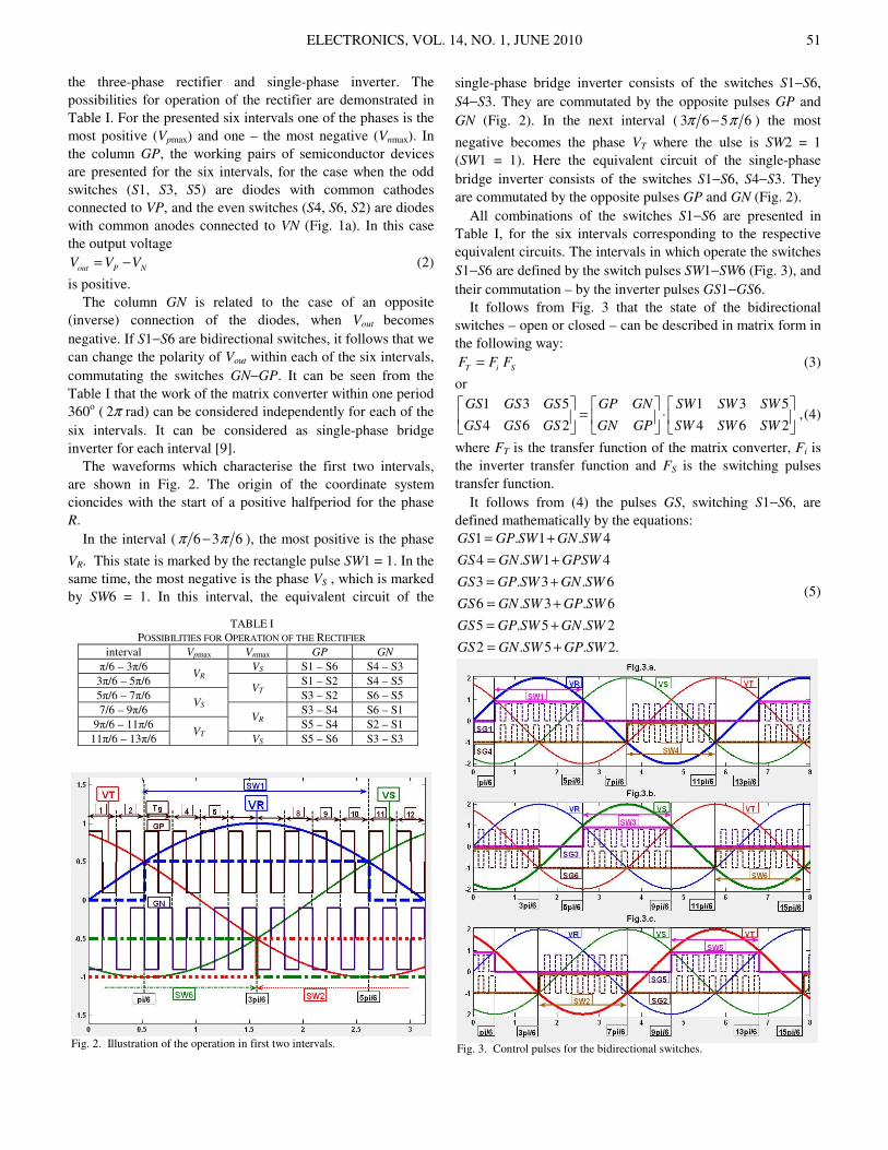
The waveforms which characterise the first two intervals, are shown in Fig. 2. The origin of the coordinate system cioncides with the start of a positive halfperiod for the phase R.

In the interval ( 6 3 6π π− ), the most positive is the phase

VR. This state is marked by the rectangle pulse SW1 = 1. In the same time, the most negative is the phase VS , which is marked by SW6 = 1. In this interval, the equivalent circuit of the

single-phase bridge inverter consists of the switches S1−S6, S4−S3. They are commutated by the opposite pulses GP and GN (Fig. 2). In the next interval ( 3 6 5 6π π− ) the most

negative becomes the phase VT where the ulse is SW2 = 1 (SW1 = 1). Here the equivalent circuit of the single-phase bridge inverter consists of the switches S1−S6, S4−S3. They are commutated by the opposite pulses GP and GN (Fig. 2).

All combinations of the switches S1−S6 are presented in Table I, for the six intervals corresponding to the respective equivalent circuits. The intervals in which operate the switches S1−S6 are defined by the switch pulses SW1−SW6 (Fig. 3), and their commutation – by the inverter pulses GS1−GS6.

It follows from Fig. 3 that the state of the bidirectional switches – open or closed – can be described in matrix form in the following way:

T i SF F F= (3)

or 1 3 5 1 3 5

4 6 2 4 6 2

GS GS GS GP GN SW SW SW

GS GS GS GN GP SW SW SW

= ⋅

, (4)

where FT is the transfer function of the matrix converter, Fi is the inverter transfer function and FS is the switching pulses transfer function.

It follows from (4) the pulses GS, switching S1−S6, are defined mathematically by the equations:

1 . 1 . 4

4 . 1 4

3 . 3 . 6

6 . 3 . 6

5 . 5 . 2

2 . 5 . 2.

GS GP SW GN SW

GS GN SW GPSW

GS GP SW GN SW

GS GN SW GP SW

GS GP SW GN SW

GS GN SW GP SW

= +

= +

= +

= +

= +

= +

(5)

TABLE I POSSIBILITIES FOR OPERATION OF THE RECTIFIER

interval Vpmax Vnmax GP GN

π/6 – 3π/6 VS S1 – S6 S4 – S3 3π/6 – 5π/6

VR S1 – S2 S4 – S5

5π/6 – 7π/6 VT

S3 – S2 S6 – S5 7/6 – 9π/6

VS S3 – S4 S6 – S1 9π/6 – 11π/6

VR S5 – S4 S2 – S1

11π/6 – 13π/6 VT

VS S5 – S6 S3 – S3

Fig. 2. Illustration of the operation in first two intervals.

Fig. 3. Control pulses for the bidirectional switches.

ELECTRONICS, VOL. 14, NO. 1, JUNE 2010 52

The equations (5) correspond to the time intervals from Fig. 3. It is seen that

1 4

3 6

5 2.

GS GS

GS GS

GS GS

=

=

=

(6)

The state of the matrix converter can be described in the following way:

P

T in

N

VF V

V

=

(7)

or 1 3 5

4 6 2P

N

V VS VS VS

V VS VS VS

= + +

= + +

, (8)

where 1 1. ; 3 3. ;

5 5. ; 4 4. ;

6 6. ; 2 2. .

R S

T R

S T

VS GS V VS GS V

VS GS V VS GS V

VS GS V VS GS V

= =

= =

= =

(9)

The single-phase output voltage (2) has thе form:

( ) ( )

( )

( ) 1 4 ( ) 3 6 ( )

5 2 ( )

out R S

T

V t GS GS V t GS GS V t

GS GS V t

= − + −

+ −

(10)

13,5...

13,5...

13,5...

1 4 .sin( ) .sin( )

2 23 6 .sin( ) .sin( )

3 3

2 25 2 .sin( ) .sin( ).

3 3

g n g

n

g n g

n

g n g

n

SW SW A t A n t

SW SW A t A n t

SW SW A t A n t

ω ω

π πω ω

π πω ω

∞

=

∞

=

∞

=

− = +

− = − + −

− = + + +

∑

∑

∑

(11)

The parameter g

ω in (11) is the commutation frequency of

the bidirectional switches. The coefficient A1 is the magnitude of the commutation function, which is assumed to be 1. The first harmonic of the Fourier expansion of A1 is of the value 4 π . The higher harmonics An have significantly lower

magnitudes and for the purposes of the performed consideration are neglected. Replacing (11) in (10), the following dependence is obtained for Vout(t) :

4( ) sin .sin

4 2 2sin( ).sin( )

3 34 2 2

sin( ).sin( ).3 3

out m g

m g

m g

V t V t t

V t t

V t t

ω ω

π

π πω ω

π

π πω ω

π

= +

+ − − +

+ − −

(12)

The obtained mathematical dependencies (1)-(10) are solved using the program MATLAB. The input voltage vector Vin is shown in Table II.

The M-files defining the inverter transfer function Fi (GP and GN) are given in Table III, where: hp is the number of the half-periods of the vector Vin; n – number of commutations of the switches S1−S6 in one half-period (n=12 – Fig. 2); N – number of points (for instance 100) for one commutation period Tg.

The computational calculation step along the X axis is:

dx=pi/(n.N), where ).(0 pihx p≤≤ . The dimension of the

vector X=x[lx] in MATLAB is defined in the main program using the command line:

x = 0: dx: (hp*pi); lx = length(x); The M-files sw1 and sw2 are given in Table IV. The rest

elements of the switching transfer function FS are described similarly.

The solution of equation (9) is shown in Fig. 4 and the solution of equations (8) and (2) is presented in Fig. 5.

TABLE II M-FILES

File function vr File function vs File function vt function y=vr(x) lx=length(x); y=zeros(size(x)) for i=1:lx y(i)=sin(x(i)); end

function y=vs(x) lx=length(x); y=zeros(size(x)); for i=1:lx y(i)=sin(x(i)+ +4*pi/3); end

function y=vt(x) lx=length(x); y=zeros(size(x)) for i=1:lx y(i)=sin(x(i)+ +2*pi/3); end

TABLE III M-FILES

File function gp File function gn function y=gp(x) lx=length(x); y=zeros(size(x)); i=0; for k=1:12*4 for j=1:100 i=100*(k-1)+j; if j<=50 y(i)=1.0; else y(i)=0.0; end end end

function y=gn(x) lx=length(x); y=zeros(size(x)); i=0; for k=1:12*4 for j=1:100 i=100*(k-1)+j; if j<=50 y(i)=0.0; else y(i)=1.0; end end end

TABLE IV M-FILES

File function sw1 File function sw2 function y=sw1(x) lx=length(x); y=zeros(size(x)); for i=1:lx if (vr(x(i))>vs(x(i))) &(vr(x(i))>vt(x(i))) y(i)=1.0; else y(i)=0.0; end end

function y=sw2(x) lx=length(x); y=zeros(size(x)); for i=1:lx if (vt(x(i))<vr(x(i))) &(vt(x(i))<vs(x(i))) y(i)=1.0; else y(i)=0.0; end end

Fig. 4. Graphical representation of the solution of the equations (9).

ELECTRONICS, VOL. 14, NO. 1, JUNE 2010

53

III. SIMULINK SIMULATION

The electrical circuit for the computer simulation of the matrix converter is shown in Fig. 6. The simulation of the

circuit is performed for a load series resonant circuit. The signals SW1−SW6, included in the switching transfer function FS, are created in the block Subsystem1. Its electrical circuit is shown in Fig. 7.

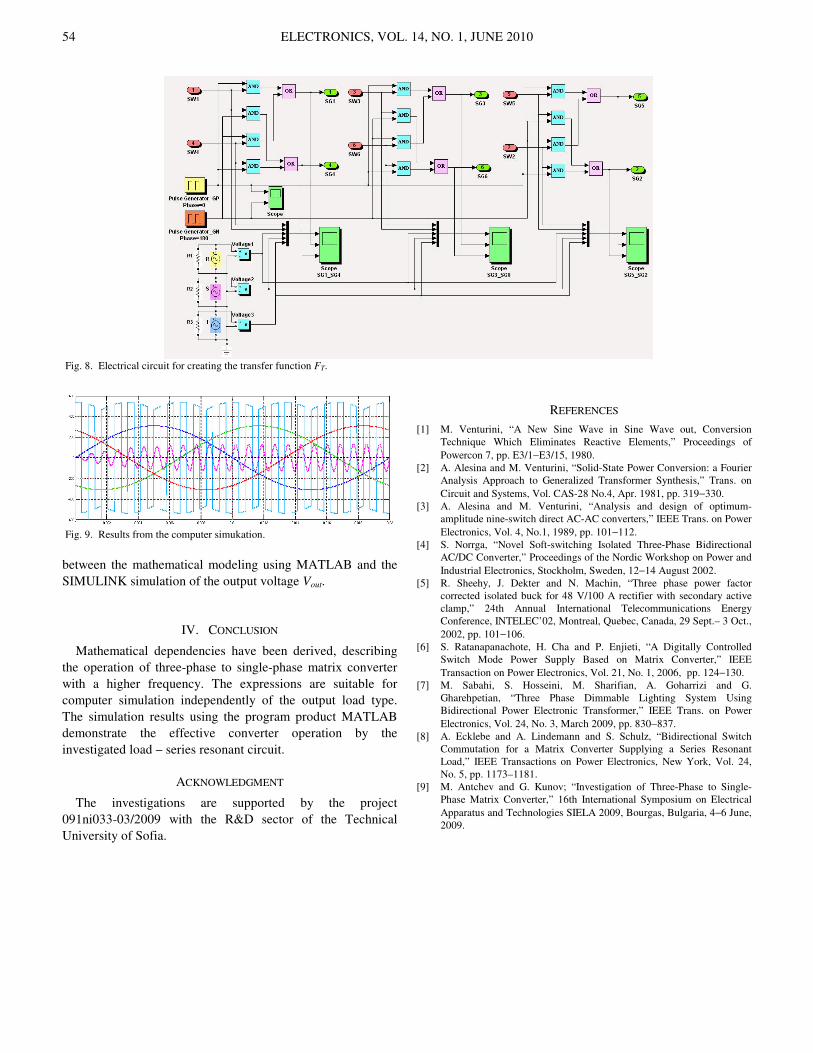
The signals GS1−GS6 included in the matrix transfer function FT are created in the block Subsystem2. Its electrical circuit is shown in Fig. 8. The functional generators Pulse Generator – GP and Pulse Generator – GN create the signals of the inverter transfer function Fi. The simulation results for the three-phase supply voltages, the output voltage and the output current of the matrix converter are shown in Fig. 9.

The sinusoidal character of the output current is represented for the so chosen RLC load. Fig. 9 illustrates a full confidence

Fig. 5. Graphical representation of the solution of the equations (8) and (2).

Fig. 6. Electrical circuit of the matrix converter represented in SIMULINK.

Fig. 7. Electrical circuit for creating the transfer function FS.

ELECTRONICS, VOL. 14, NO. 1, JUNE 2010 54

between the mathematical modeling using MATLAB and the SIMULINK simulation of the output voltage Vout.

IV. CONCLUSION

Mathematical dependencies have been derived, describing the operation of three-phase to single-phase matrix converter with a higher frequency. The expressions are suitable for computer simulation independently of the output load type. The simulation results using the program product MATLAB demonstrate the effective converter operation by the investigated load – series resonant circuit.

ACKNOWLEDGMENT

The investigations are supported by the project 091ni033-03/2009 with the R&D sector of the Technical University of Sofia.

REFERENCES

[1] M. Venturini, “A New Sine Wave in Sine Wave out, Conversion Technique Which Eliminates Reactive Elements,” Proceedings of Powercon 7, pp. E3/1−E3/15, 1980.

[2] A. Alesina and M. Venturini, “Solid-State Power Conversion: a Fourier Analysis Approach to Generalized Transformer Synthesis,” Trans. on Circuit and Systems, Vol. CAS-28 No.4, Apr. 1981, pp. 319−330.

[3] A. Alesina and M. Venturini, “Analysis and design of optimum-amplitude nine-switch direct AC-AC converters,” IEEE Trans. on Power Electronics, Vol. 4, No.1, 1989, pp. 101−112.

[4] S. Norrga, “Novel Soft-switching Isolated Three-Phase Bidirectional AC/DC Converter,” Proceedings of the Nordic Workshop on Power and Industrial Electronics, Stockholm, Sweden, 12−14 August 2002.

[5] R. Sheehy, J. Dekter and N. Machin, “Three phase power factor corrected isolated buck for 48 V/100 A rectifier with secondary active clamp,” 24th Annual International Telecommunications Energy Conference, INTELEC’02, Montreal, Quebec, Canada, 29 Sept.– 3 Oct., 2002, pp. 101−106.

[6] S. Ratanapanachote, H. Cha and P. Enjieti, “A Digitally Controlled Switch Mode Power Supply Based on Matrix Converter,” IEEE Transaction on Power Electronics, Vol. 21, No. 1, 2006, pp. 124−130.

[7] M. Sabahi, S. Hosseini, M. Sharifian, A. Goharrizi and G. Gharehpetian, “Three Phase Dimmable Lighting System Using Bidirectional Power Electronic Transformer,” IEEE Trans. on Power Electronics, Vol. 24, No. 3, March 2009, pp. 830−837.

[8] A. Ecklebe and A. Lindemann and S. Schulz, “Bidirectional Switch Commutation for a Matrix Converter Supplying a Series Resonant Load,” IEEE Transactions on Power Electronics, New York, Vol. 24, No. 5, pp. 1173–1181.

[9] M. Antchev and G. Kunov; “Investigation of Three-Phase to Single-Phase Matrix Converter,” 16th International Symposium on Electrical Apparatus and Technologies SIELA 2009, Bourgas, Bulgaria, 4−6 June, 2009.

Fig. 8. Electrical circuit for creating the transfer function FT.

Fig. 9. Results from the computer simukation.