computer science, eth zurichcomputer science, eth zurich mohsen ghaffari march 2019. ii. contents...

D istributed Graph Algorithms

Computer Science, ETH Zurich

Mohsen Ghaffari

March 2019

CONTENTS iii

Contents

1 Local Problems 11.1 The Distributed LOCAL Model . . . . . . . . . . . . . . . . . 2

1.2 Coloring Rooted Trees . . . . . . . . . . . . . . . . . . . . . . . 2

1.2.1 3-Coloring Rooted Trees in log∗ n+O(1) Rounds . . 4

1.2.2 3-Coloring Rooted Trees Needs 12 log∗ n−O(1) Rounds 6

1.3 Coloring Unrooted Trees . . . . . . . . . . . . . . . . . . . . . 8

1.3.1 The Lower Bound . . . . . . . . . . . . . . . . . . . . . 9

1.3.2 The Upper Bound . . . . . . . . . . . . . . . . . . . . . 10

1.4 Deterministic Coloring of General Graphs . . . . . . . . . . 11

1.4.1 Take 1: Linial’s Coloring Algorithm . . . . . . . . . . 11

1.4.2 Take 2: Kuhn-Wattenhofer Coloring Algorithm . . . 15

1.4.3 Take 3: Kuhn’s Algorithm via Defective Coloring . . 16

1.5 Network Decomposition . . . . . . . . . . . . . . . . . . . . . 18

1.5.1 Definition and Applications . . . . . . . . . . . . . . . 18

1.5.2 Randomized Construction . . . . . . . . . . . . . . . . 20

1.5.3 Deterministic Construction . . . . . . . . . . . . . . . 22

1.6 Maximal Independent Set . . . . . . . . . . . . . . . . . . . . 25

1.6.1 Definition and Reductions . . . . . . . . . . . . . . . . 25

1.6.2 Luby’s MIS Algorithm . . . . . . . . . . . . . . . . . . 26

1.7 Sublogarithmic-Time Randomized Coloring . . . . . . . . . 29

1.7.1 The algorithm for low-degree graphs . . . . . . . . . 29

1.7.2 The extension to high-degree graphs . . . . . . . . . 30

1.8 Exercises . . . . . . . . . . . . . . . . . . . . . . . . . . . . . . . 32

iv CONTENTS

Chapter 1

Local Problems

1

2 CHAPTER 1. LOCAL PROBLEMS

1.1 The Distributed LOCAL Model

We work with the LOCAL model, which was first formalized by Linial [Lin87,Lin92]. The model definition is as follows.

Definition 1.1. (The LOCAL model) We consider an arbitrary n-node graphG = (V ,E) where V = 1, 2, . . . ,n, which abstracts the communication network.Unless noted otherwise, G is a simple, undirected, and unweighted graph. Thereis one process on each node v ∈ V of the network. At the beginning, the processesdo not know the graph G, except for knowing1 n, and their own unique identifierin 1, 2, . . . ,n. The algorithms work in synchronous rounds. Per round, eachnode/process performs some computation based on its own knowledge, and thensends a message to all of its neighbors, and then receives the messages sent to it byits neighbors in that round. In each graph problem in this model, we require thateach node learns its own part of the output, e.g., its own color in a graph coloring.

Comment: We stress that the model does not assume any limitation onthe size of the messages, or on the computational power of the processes.Because of this, it is not hard to see that, any t-round algorithm in theLOCAL model induces a function which maps the t-hop neighborhoodof each node to its output (why?). For instance, a t-round algorithm forgraph coloring maps the topology induced by vertices within distance t ofa vertex v to the coloring of vertex v. The converse of this statement is alsotrue, meaning that if for a given graph problem, such a function exists,then there is also a t-round algorithm for solving that problem. Hence,one can say that the LOCAL model captures the locality of graph problemsin a mathematical sense.

Observation 1.2. Any graph problem on any n-node graph G can be solved inO(n) rounds. In fact, using D to denote the diameter of the graph, any problemcan be solved in O(D) rounds.

1.2 Coloring Rooted Trees

We start by examining the graph coloring problem, and in a very specialcase, coloring rooted trees. This basic-looking problem already turns outto have some quite interesting depth, as we see in this section.

1Most often, the algorithms will use only the assumption that nodes know an upperbound N on n such that N ∈ [n,nc] for a small constant c > 1.

1.2. COLORING ROOTED TREES 3

The setting is as follows. We consider an arbitrary rooted tree T = (V ,E),such that V = 1, 2, . . . ,n, and where each node v knows its parent p(v)in T . The objective is to find a proper coloring of T , that is, a colorassignment φ : V → 1, 2, . . . ,q such that there does not exist any node vwith φ(v) = φ(p(v)). Of course, we are interested in using a small numberof colors q, and we seek fast algorithms for computing such a coloring,that is, algorithms that use a small number of rounds.

Clearly, each tree can be colored using just 2 colors. However, comput-ing a 2-coloring in the LOCAL model is not such an interesting problem,due to the following simple observation:

Observation 1.3. Any LOCAL algorithm for 2-coloring an n-node directed pathrequires at least Ω(n) rounds.

In contrast, 3-coloring has no such unfortunate lower bound, and infact, entails something quite non-trivial: it has a tight round complexity of12 log∗ n±O(1). Recall the definition of the log-Star function:

log∗(x) =

0 if x 6 11+ log∗(log x) if x > 1

To prove this tight 12 log∗ n±O(1) round complexity, in the next two

subsections, we explain the following two directions of this result:

• First, in Section 1.2.1, we explain a log∗ n+O(1) round algorithmfor 3-coloring rooted trees. The upper bound can actually be im-proved to 1

2 log∗ n+O(1) rounds [SV93], and even to exactly 12 log∗ n

rounds [RS14], but we do not cover those refinements. There are fourknown methods for obtaining O(log∗ n)-round algorithms [CV86,SV93, NS93, FHK16]. The algorithm we describe is based on anidea of [NS95] and some extra step from [GPS87]. The approach of[CV86] will be covered in Exercise 1.1.

• Then, in Section 1.2.2, we prove the above bound to be essentiallyoptimal by showing that any deterministic algorithm for 3-coloringrooted trees requires at least 12 log∗ n−O(1) rounds. This result wasfirst proved by [Lin87, Lin92]. We explain a somewhat streamlinedproof, based on [LS14]. The lower bound holds also for randomizedalgorithms [Nao91], but we will not cover that generalization, for thesake of simplicity. Furthermore, essentially the same lower boundcan be obtained as a direct corollary of Ramsey Theory. We will havea brief explanation about that, at the end of this subsection.


1.2.1 3-Coloring Rooted Trees in log∗ n+O(1) Rounds

Theorem 1.4. Any n-node rooted-tree can be colored with 3 colors, in log∗ n+

O(1) rounds.

Notice that the initial numbering 1, 2, . . . , n of the vertices is already acoloring with n colors. We explain a method for gradually improving thiscoloring, by iteratively reducing the number of colors. The key ingredientis a single-round color-reduction method, based on Sperner families, whichachieves the following:

Lemma 1.5. Given a k-coloring φold of a rooted tree where k > C0 for a constant2

C0, in a single round, we can compute a k ′-coloring φnew, for k ′ = logk +log log k/2+ 1.

Proof. Let each node u send its color φold(u) to its children. We nowdescribe a method which allows each node v to compute its new coloringφnew(v), based on φold(v) and φold(u) where u is the parent of v, with nofurther communication.

Consider an arbitrary one-to-one mapping M : 1, 2, . . . ,k→ Fk ′ , fixeda priori, where Fk ′ denotes the set of all the subset of size k ′/2 of the set1, 2, . . . ,k ′. Notice that such a one-to-one mapping exists, because

|Fk ′ | =

(k ′

k ′/2

)> 2k

′/√2k ′ > k.

For each node v, we compute the new color φnew(v) ∈ 1, 2, . . . ,k ′ of v asfollows. Let u be the parent of v. Since both M(φold(v)) and M(φold(u)) aresubsets of size k ′/2, and because φold(v) 6= φold(u) and M is a one-to-onemapping, we know that M(φold(v)) \M(φold(u)) 6= ∅. Let φnew(v) be anyarbitrary color in M(φold(v)) \M(φold(u)). Since each node v gets a colorφnew(v) ∈ M(φold(v)) \M(φold(u)) that is not in the color set M(φold(u))

of its parent, φnew(v) 6= φnew(u) ∈ M(φold(u)). Hence, φnew is a propercoloring.

Remark 1.1. Notice that in the above proof, the main property that we used isthat none of the color-sets M(i) ∈ Fk ′ is contained in another M(j) ∈ Fk ′ , fori 6= j. Generally, a family of sets such that none of them is contained in anotheris called a Sperner Family. In particular, `-element subsets of a k ′-element set

2We assume this constant lower bound C0 mainly to simplify our job and let us notworry about the rounding issues.


form a Sperner family, the size of which is maximized by setting ` = bk ′/2c, as wedid above. More generally, Sperner’s theorem shows that any Sperner family ona ground set of size k ′ has size at most

(k ′

bk ′/2c)

[Spe28]. See [Lub66] for a shortand cute proof of Sperner’s theorem, via a simple double counting.

We can now iteratively apply the above method, abstracted in thestatement of Lemma 1.5, to reduce the number of colors. After one round,we go from an initial n-coloring to a (logn + log logn/2 + 1)-coloring.After one more round, we get to a coloring which has no more thanlog logn+O(log log logn) colors. More generally, after at most log∗ n+

O(1) repetitions, we get to a coloring with no more than C0 colors, for aconstant C0. At this point, we cannot apply the above routine anymore.However, we can use an easier method that repeatedly uses two roundsto shave off one color, until arriving at a 3-coloring. We explain this next.Overall, we use log∗ n+O(1) rounds to get a 3-coloring.

Lemma 1.6. Given a k-coloring φold of a rooted tree where k > 4, in two rounds,we can compute a (k− 1)-coloring φnew.

Proof. First, use one round where each node u sends its color φold(u) to itschildren. Then, let each node v set its temporary coloring φ ′old(v) = φold(u),where u is the parent of v. For the root node r, this rule is not well-defined.But that is easy to fix. Define φ ′old(r) ∈ 1, 2, 3 \φold(r). Observe that φ ′oldis a proper k-coloring, with the following nice additional property: foreach node u, all of its children have the same color φ ′old(u).

Now, use another round where each node u sends its color φ ′old(u) toits children. Then, define the new color φnew(v) as follows. For each nodev such that φ ′old(v) 6= k, let φnew(v) = φ ′old(v). For each node v such thatφ ′old(v) = k, let φnew(v) be a color in 1, 2, 3 \ φ ′old(u),φold(v).

Notice that since only nodes of color k are changing their color, thesenodes are non-adjacent. Each of them switches to a color that is differentthan what is held by its parent and its children. Hence, the new coloringφnew(v) is proper.

Proof of Theorem 1.4. The proof follows by applying Lemma 1.5 for log∗ n+

O(1) iterations, until getting to a coloring with no more than C0 = O(1)

colors, and then applying the method of Lemma 1.6 for C0 − 3 = O(1)

iterations, until getting to a 3-coloring.


1.2.2 3-Coloring Rooted Trees Needs 12

log∗ n−O(1) Rounds

Theorem 1.7. Any deterministic algorithm for 3-coloring n-node directed pathsneeds at least log∗ n

2 − 2 rounds.

For the sake of contradiction, suppose that there is an algorithm A

that computes a 3-coloring of any n-node directed path in t rounds fort <

log∗ n2 − 2. When running this algorithm for t rounds, any node v can

see at most the k-neighborhood around itself for k = 2t+ 1, that is, thevector of identifiers for the nodes up to t hops before itself and up to thops after itself. Hence, if the algorithm A exists, there is a mapping fromeach such neighborhood to a color in 1, 2, 3 such that neighborhoods thatcan be conceivably adjacent are mapped to different colors.

We next make this formal by a simple and abstract definition. Forsimplicity, we will consider only a restricted case of the problem wherethe identifiers are set monotonically increasing along the path. Notice thisrestriction only strengthens the lower bound, as it shows that even for thisrestricted case, there is no t-round algorithm for t < log∗ n

2 − 2.

Definition 1.8. We say B is a k-ary q-coloring if for any set of identifiers1 6 a1 < a2 < · · · < ak < ak+1 6 n, we have the following two properties:

P1: B(a1,a2, . . . ,ak) ∈ 1, 2, . . . ,q,

P2: B(a1,a2, . . . ,ak) 6= B(a2, . . . ,ak+1).

Observation 1.9. If there exists a deterministic algorithm A for 3-coloring n-node directed paths in t < log∗ n

2 − 2 rounds, then there exists a k-ary 3-coloringB, where k = 2t+ 1 < log∗ n− 3.

Proof. Suppose that such an algorithm A exists. We then produce a k-ary3-coloring B by examining A. For any set of identifiers 1 6 a1 < a2 < · · · <ak 6 n, define B(a1,a2, . . . ,ak) as follows. Simulate algorithm A on animaginary directed path where a consecutive portion of the identifiers onthe path are set equal to a1,a2, . . . ,ak. Then, let B(a1,a2, . . . ,ak) be equalto the color in 1, 2, 3 that the node at+1 receives in this simulation.

We now argue that B as defined above is a k-ary 3-coloring. Prop-erty P1 holds trivially. We now argue that property P2 also holds. Forthe sake of contradiction, suppose that it does not, meaning that thereexist a set of identifiers 1 6 a1 < a2 < · · · < ak < ak+1 6 n such thatB(a1,a2, . . . ,ak) = B(a2, . . . ,ak+1). Then, imagine running algorithm A on


an imaginary directed path where a consecutive portion of identifiers areset equal to a1,a2, . . . ,a2t+2. Then, since B(a1,a2, . . . ,ak) = B(a2, . . . ,ak+1),the algorithm A assigns the same color to at+1 and at+2. This is in contra-diction with A being a 3-coloring algorithm.

To prove Theorem 1.7, we show that a k-ary 3-coloring B where k <log∗ n− 3 cannot exist. The proof is based on the following two lemmas:

Lemma 1.10. There is no 1-ary q-coloring with q < n.

Proof. A 1-ary q-coloring requires that B(a1) 6= B(a2), for any two identi-fiers 1 6 a1 < a2 6 n. By the Pigeonhole principle, this needs q > n.

Lemma 1.11. If there is a k-ary q-coloring B, then there exists a (k− 1)-ary2q-coloring B ′.

Proof. For any set of identifiers 1 6 a1 < a2 < · · · < ak−1 6 n, defineB ′(a1,a2, . . . ,ak−1) to be the set of all possible colors i ∈ 1, . . . ,q for which∃ak > ak−1 such that B(a1,a2, . . . ,ak−1,ak) = i.

Notice that B ′ is a subset of 1, . . . ,q. Hence, it has 2q possibilities,which means that B ′ has property P1 and it assigns each set of identifiers1 6 a1 < a2 < · · · < ak−1 6 n to a number in 2q. Now we argue that B ′ alsosatisfies property P2.

For the sake of contradiction, suppose that there exist identifiers 1 6a1 < a2 < · · · < ak 6 n such that B ′(a1,a2, . . . ,ak−1) = B ′(a2,a3, . . . ,ak).Let q∗ = B(a1,a2, . . . ,ak) ∈ B ′(a1,a2, . . . ,ak−1). Then, we must have q∗ ∈B ′(a2,a3, . . . ,ak). Thus, ∃ak+1 > ak such that q∗ = B(a2,a3, . . . ,ak,ak+1).But, this means B(a1,a2, . . . ,ak) = q∗ = B(a2,a3, . . . ,ak,ak+1), which isin contradiction with B being a k-ary q-coloring. Having reached at acontradiction by assuming that B ′ does not satisfy P2, we conclude that itactually does satisfy P2. Hence, B ′ is a (k− 1)-ary 2q-coloring.

Proof of Theorem 1.7. For the sake of contradiction, suppose that there isan algorithm A that computes a 3-coloring of any n-node directed pathin t rounds for t 6 log∗ n

2 − 2. As stated in Observation 1.9, if there existsan algorithm A that computes a 3-coloring of any n-node directed pathin t rounds for t 6 log∗ n

2 − 2, then there exists a k-ary 3-coloring B, wherek = 2t+ 1 < log∗ n− 3. Using one iteration of Lemma 1.11, we wouldget that there exists a (k − 1)-ary 8-coloring. Another iteration wouldimply that there exists a (k − 2)-ary 28-coloring. Repeating this, afterk < log∗ n− 3 iterations, we would get a 1-ary coloring with less than n


colors. However, this is in contradiction with Lemma 1.10. Hence, such analgorithm A cannot exist.

An Alternative Lower Bound Proof Via Ramsey Theory:Let us first briefly recall the basics of Ramsey Theory. The simplest caseof Ramsey’s theorem says that for any `, there exists a number R(`) suchthat for any n > R(`), if we color the edges of the n-node complete graphKn with two colors, there exists a monochromatic clique of size ` in it,that is, a set of ` vertices such that all of the edges between them have thesame color. A simple example is that among any group of at least 6 = R(3)people, there are either at least 3 of them which are friends, or at least 3 ofthem no two of which are friends.

A similar statement is true in hypergraphs. Of particular interest forour case is coloring hyperedges of a complete n-vertex hypergraph ofrank k, that is, the hypergraph where every subset of size k of the verticesdefines one hyperedge. By Ramsey theory, it is known that there existsan n0 such that, if n > n0, for any way of coloring hyperedges of thecomplete n-vertex hypergraph of rank k with 3 colors, there would be amonochromatic clique of size k+ 1. That is, there would be a set of k+ 1vertices a1, . . . , ak in 1, . . . ,n such that all of their

(k+1k

)= k subsets with

cardinality k have the same color.In particular, consider an arbitrary k-ary coloring B, and let B define the

colors of the hyperedges a1, . . . ,ak when 1 6 a1 < a2 < · · · < ak 6 n. Forthe remaining hyperedges, color them arbitrarily. By Ramsey’s theorem,we would get the following: there exist vertices 1 6 a1 < a2 < · · · < ak <ak+1 6 n such that B assigns the same color to hyperedges a1, . . . ,akand a2, . . . ,ak+1. But this is in contradiction with the property P2 of Bbeing a k-ary coloring. The value of n0 that follows from Ramsey theoryis such that k = O(log∗ n0). In other words, Ramsey’s theorem rules outo(log∗ n)-round 3-coloring algorithms for directed paths. See [CFS10] formore on hypergraph Ramsey numbers.

1.3 Coloring Unrooted Trees

In the previous sections, we saw that on a rooted tree, where each nodeknows its parent, a 3-coloring can be computed distributedly in O(log∗ n)rounds. Moreover, we proved that this round complexity is optimal. ThisO(log∗ n)-round algorithm for rooted trees heavily relies on each nodeknowing its parent.

1.3. COLORING UNROOTED TREES 9

We next prove that no such result is possible in unrooted trees, whennodes do not know which neighbor is their parent. More concretely, weprove that any deterministic algorithm for coloring unrooted trees that runsin o(log∆ n) rounds must use at least Ω(∆/ log∆) colors. Moreover, wecomplement this by showing that given O(logn) rounds, we can computea 3-coloring of any n-node tree.

1.3.1 The Lower Bound

Theorem 1.12. Any (deterministic) distributed algorithm A that colors n-nodetrees with maximum degree ∆ using less than o(∆/ log∆) colors has roundcomplexity at least Ω(log∆ n).

To prove the claimed lower bound, we will use a graph-theoretic resultabout the existence of certain graphs. The proof of this lemma is basedon a probabilistic method argument, but we do not cover it in this lecture.Before stating the properties of this graph, we recall that the girth of agraph is the length of the shortest cycle.

Fact 1.13 (Bollobas [Bol78]). There exists an n-node graph H∗ where all nodeshave degree ∆, with girth g(H∗) = Ω(log∆ n) and chromatic number χ(H∗) =Ω(∆/ log∆).

Remark 1.2. We note that this lower bound on the chromatic number is asymp-totically tight, because high-girth graphs, and more generally triangle-free graphs,with maximum degree ∆ have chromatic number O(∆/ log∆) [Kim95, Jam11,PS15].

Proof of Theorem 1.12. For the sake of contradiction, suppose that thereexists a deterministic distributed algorithm A that computes a o(∆/ log∆)-coloring of any n-node tree with maximum degree ∆, in o(log∆ n) rounds.

We run A on the graph H∗, stated in Fact 1.13. Notice that H∗ is nota tree. However, since g(H∗) = Ω(log∆ n), within the o(log∆ n) rounds ofthe algorithm, no one will notice! In particular, since g(H∗) = Ω(log∆ n),for any node v, the subgraph Tv of H∗ induced by nodes within distanceo(log∆ n) of v is a tree (why?). Thus, within the o(log∆ n) rounds of thealgorithm, node v will think that the algorithm A is being run on Tv andwill not realize that the algorithm is being run on a non-tree graph H∗.Similarly, none of the nodes will recognize that we are not on a tree.Hence, each node v will compute an output as if the algorithm A was


being run on its local tree Tv. This must produce a valid coloring of H∗ witho(∆/ log∆) colors. That is because if the algorithm creates two neighborsv and u with the same color, then running the algorithm on the tree Tvwould also produce a non-valid color. However, the fact that A is able tocompute a o(∆/ log∆)-coloring of H∗ is in contradiction with the fact thatχ(H∗) = Ω(∆/ log∆).

1.3.2 The Upper Bound

Theorem 1.14. There is a deterministic distributed algorithm that computes a3-coloring of any n-node tree in O(logn) rounds.

The Algorithm for Coloring Unrooted Trees, Step 1 We first performan iterated peeling process, on the given tree T = (V ,E). Let T1 = T andlet layer L1 be the set of all vertices of T1 whose degree in T1 is at most2. Then, let T2 = T1 \ L1 be the forest obtained by removing from T1 allthe L1 vertices. Then, define layer L2 be the set of all vertices of T2 whosedegree in T2 is at most 2. Then, define T3 = T2 \ L2 similar to before. Moregenerally, each Ti+1 is defined as Ti+1 = Ti \ Li, which is the forest obtainedby removing from Ti all the layer Li vertices, and then layer Li+1 is definedto be the vertices that have degree at most 2 in Ti+1.

Lemma 1.15. The process terminates in O(logn) iterations, meaning that Vgets decomposed into disjoint sets L1, L2, . . . , L` for some ` = O(logn).

Proof. Ti has at most |Ti|− 1 edges, since it is a forest. Hence, the numberof vertices of Ti that have degree at least 3 is at most (2|Ti|− 1)/3. Hence,at least 1/3 of the nodes of Ti are put in Li. This means in each iterationthe number of nodes reduces by a 2/3-factor, which implies that we aredone within ` = log3/2 n iterations.

The Algorithm for Coloring Unrooted Trees, Step 2 Now, we coloreach of the subgraphs T [Li] independently using 3 colors, in O(log∗ n)rounds. Notice that this is doable for instance using the algorithm fromTheorem 1.4, because T [Li] has maximum degree at most 2. We use thesecolors of the graphs T [Li] mainly as a schedule-color, for computing the finaloutput coloring of the vertices.

1.4. DETERMINISTIC COLORING OF GENERAL GRAPHS 11

The Algorithm for Coloring Unrooted Trees, Step 3 We process thegraph by going through the layers L` to L1, spending 3 rounds on each.Each time, we make sure that we have a valid final-coloring of the graphT [∪`j=iLi] with 3 colors, for decreasing value of i.

Suppose we have an arbitrary final-coloring of T [∪`j=i+1Lj] already, with3 colors. How do we compute a 3-coloring for vertices of Li in a mannerthat does not create a violation with the colors of vertices of T [∪`j=i+1Lj]?

This can be done easily using our usual trick of applying one coloringas a schedule for computing another coloring. In particular, we will solvethis part of the problem in 3 rounds. We go through the 3 schedule-colorsq ∈ 1, 2, 3 of T [Li], one by one, each time picking a final-color in 1, 2, 3 forall the vertices in Li with schedule color q.

1.4 Deterministic Coloring of General Graphs

1.4.1 Take 1: Linial’s Coloring Algorithm

In the previous section, we discussed distributed LOCAL algorithms forcoloring oriented trees. In this section, we start the study of LOCALcoloring algorithms for general graphs. Throughout, the ultimate goalwould be to obtain (∆+ 1)-coloring of the graphs — that is, an assignmentof colors 1, 2, . . . ,∆ + 1 to vertices such that no two adjacent verticesreceive the same color — where ∆ denotes the maximum degree. Noticethat by a simple greedy argument, each graph with maximum degree atmost ∆ has a (∆+ 1)-coloring: color vertices one by one, each time pickinga color which is not chosen by the already-colored neighbors. However,this greedy argument does not lead to an efficient LOCAL procedure forfinding such a coloring3.

In this section, we start with presenting an O(log∗ n)-round algorithmthat computes a O(∆2) coloring. This algorithm is known as Linial’scoloring algorithm [Lin87, Lin92]. In Section 1.4.2, we see how to transformthis coloring into a (∆+ 1)-coloring.

Theorem 1.16. There is a deterministic distributed algorithm in the LOCALmodel that colors any n-node graph G with maximum degree ∆ using O(∆2)colors, in O(log∗ n) rounds.

3The straightforward transformation of this greedy approach to the LOCAL modelwould be an algorithm that may need Ω(n) rounds.


Intuitive Discussion. Conceptually, the algorithm can be viewed4 asa more general variant of the algorithm we discussed in Section 1.2.1.In particular, the core piece is a single-round color reduction method,conceptually similar to that of Lemma 1.5. However, here, each node hasto ensure that the color it picks is different than all of its neighbors, andnot just its parents. For that purpose, we will work with a generalizationof Sperner families (as mentioned in Remark 1.1 and used in Lemma 1.5),which we describe next.

Definition 1.17. (Cover free families) Given a ground set 1, 2, . . . ,k ′, afamily of sets S1, S2, . . . , Sk ⊆ 1, 2, . . . ,k ′ is called a ∆-cover free family if foreach set of indices i0, i1, i2, . . . , i∆ ∈ 1, 2, . . . ,k, we have Si0 \

(∪∆j=1 Sij

)6= ∅.

That is, if no set in the family is a subset of the union of ∆ other sets.

Notice that in particular, a Sperner family (as discussed in Remark 1.1)is simply a 1-cover free family, i.e., no set is a subset of any other set.

Using cover free families for color reduction. Given this definition, andthe single-round color reduction method that we saw in Lemma 1.5 forrooted trees using Sperner families, the reader can already see the analo-gous single-round color reduction method for general graphs using coverfree families. This new single-color reduction will allow us to trans-form any k-coloring to a k ′-coloring. This will be elaborated later on inLemma 1.20. We would like to have k ′ as small as possible, as a function ofk and ∆. In the following, we prove the existence of ∆-cover free familieswith a small enough ground set size k ′. In particular, Lemma 1.18 achievesk ′ = O(∆2 logk) and Lemma 1.19 shows that this bound can be improvedto k ′ = O(∆2), if k 6 ∆3.

Lemma 1.18. (Existence of cover free families) For any k and ∆, there existsa ∆-cover free family of size k on a ground set of size k ′ = O(∆2 logk).

Proof. We use the probabilistic method [AS04] to argue that there existsa ∆-cover free family of size k on a ground set of size k ′ = O(∆2 logk).Let k ′ = C∆2 logk for a sufficiently large constant C > 2. For each i ∈1, 2, . . . ,k, define each set Si ⊂ 1, 2, . . . ,k ′ randomly by including eachelement q ∈ 1, 2, . . . ,k ′ in Si with probability p = 1/∆. We argue that this

4This intuitive discussion is written for a reader who has already read Lemma 1.5Otherwise, please feel free to ignore the comparisons with Sperner families and just readthe definition of cover free families and how they are applies.


random construction is indeed a ∆-cover free family, with probability closeto 1. Therefore, such a cover free family exists.

First, consider an arbitrary set of indices i0, i1, i2, . . . , i∆ ∈ 1, 2, . . . ,k.We would like to argue that Si0 \

(∪∆j=1 Sij

)6= ∅. For each element q ∈

1, 2, . . . ,k ′, the probability that q ∈ Si0 \(∪∆j=1 Sij

)is at exactly 1

∆(1−1∆)∆ >

14∆ . Hence, the probability that there is no such element q that is inSi0 \

(∪∆j=1 Sij

)is at most (1− 1

4∆)k ′ 6 exp(−C∆ logk/4). This is an upper

bound on the probability that for a given set of indices i0, i1, i2, . . . , i∆ ∈1, 2, . . . ,k, the respective sets violate the cover-freeness property thatSi0 \

(∪∆j=1 Sij

)6= ∅.

There are k(k−1∆

)way to choose such a set of indices i0, i1, i2, . . . , i∆ ∈

1, 2, . . . ,k, k ways for choosing the central index i0 and(k−1∆

)ways for

choosing the indices i1, i2, . . . , i∆. Hence, by a union bound over all thesechoices, the probability that the construction fails is at most

k

(k− 1

∆

)· exp(−C∆ logk/4) 6 k(

e(k− 1)

∆)∆ · exp(−C∆ logk/4)

6 exp(

logk+∆(logk+ 1) −C∆ logk/4)

6 exp(−C∆ logk/8) 1,

for a sufficiently large constant C. That is, the random constructionsucceeds to provide us with a valid ∆-cover free family with a positiveprobability, and in fact with a probability close to 1. Hence, such a ∆-coverfree family exists.

Lemma 1.19. For any k and ∆ > k1/3, there exists a ∆-cover free family of sizek on a ground set of size k ′ = O(∆2).

Proof. Here, we use an algebraic proof based on low-degree polynomials.Let q be a prime number that is in [3∆, 6∆]. Notice that such a primenumber exists by Bertrand’s postulate (also known as Bertrand-ChebyshevTheorem). Let Fq denote the prime field5 of order q (i.e., integers moduloq). For each i ∈ 1, 2, . . . ,k, associate with set Si — to be constructed —a distinct degree d = 2 polynomial gi : Fq → Fq over Fq. Notice thatthere are qd+1 > ∆3 > k such polynomials and hence such an associationis possible. Let Si be the set of all evaluation points of gi, that is, letSi = (a,gi(a)) |a ∈ Fq. These are subsets of the k ′ = q2 cardinality setFq ×Fq. Notice two key properties:

5See https://en.wikipedia.org/wiki/Finite_field

https://en.wikipedia.org/wiki/Finite_field


(A) for each i ∈ 1, 2, . . . ,k, we have |Si| = q.

(B) for each i, i ′ ∈ 1, 2, . . . ,k such that i 6= i ′, we have |Si ∩ Si ′ | 6 d.

The latter property holds because, in every intersection point, the degreed polynomial gi − gi ′ evaluates to zero, and each degree d polynomial hasat most d zeros. Now, the ∆ cover-freeness property follows trivially from(A) and (B), because for any set of indices i0, i1, i2, . . . , i∆ ∈ 1, 2, . . . ,k, wehave

|Si0 \(∪∆j=1 Sij

)| > |Si0 | −

∆∑j=1

|Si0 ∩ Sij |

> q − ∆ · d = q− 2∆ > ∆ > 1.

Remark 1.3. One can easily generalize the construction of Lemma 1.19, by takinghigher-degree polynomials, to a ground set of size k ′ = O(∆2 log2∆ k), where noassumption on the relation between k and ∆ would be needed.

Lemma 1.20. Given a k-coloring φold of a graph with maximum degree ∆,in a single round, we can compute a k ′-coloring φnew, for k ′ = O(∆2 logk).Furthermore, if k 6 ∆3, then the bound can be improved to k ′ = O(∆2).

Proof Sketch. Follows from the existence of cover free families as proven inLemma 1.18 and Lemma 1.19. Namely, each node v of old color φold(v) = qfor q ∈ 1, . . . ,k will use the set Sq ⊆ 1, . . . ,k ′ in the cover free family asits color-set. Then, it sets its new color φnew(v) = q ′ for a q ′ ∈ Sq such thatq ′ is not in the color-set of any of the neighbors.

Proof of Theorem 1.16. The proof is via iterative applications of Lemma 1.20.We start with the initial numbering of the vertices as a straightforwardn-coloring. With one application of Lemma 1.20, we transform this intoa O(∆2 logn) coloring. With another application, we get a coloring withO(∆2(log∆+ log logn)) colors. With another application, we get a coloringwith O(∆2(log∆+ log log logn)) colors. After O(log∗ n) applications, weget a coloring with O(∆2 log∆) colors (why6?). At this point, we use oneextra iteration, based on the second part of Lemma 1.20, which gets us toan O(∆2)-coloring.

6If this is not clear, please ask during the exercise sessions.


1.4.2 Take 2: Kuhn-Wattenhofer Coloring Algorithm

In the previous section, we saw an O(log∗ n)-round algorithm for com-puting a O(∆2)-coloring. In this section, we explain how to transformthis into a (∆+ 1)-coloring. We will first see a very basic algorithm thatperforms this transformation in O(∆2) rounds. Then, we see how withthe addition of a small but clever idea of [KW06], this transformationcan be performed in O(∆ log∆) rounds. As the end result, we get anO(∆ log∆+ log∗ n)-round algorithm for computing a (∆+ 1)-coloring.

Warm up: One-By-One color Reduction

Lemma 1.21. Given a k-coloring φold of a graph with maximum degree ∆ wherek > ∆+ 2, in a single round, we can compute a (k− 1)-coloring φnew.

Proof. For each node v such that φold(v) 6= k, set φnew(v) = φold(v). Foreach node v such that φold(v) = k, let node v set its new color φnew(v)to be a color q ∈ 1, 2, . . . ,∆+ 1 such that q is not taken by any of theneighbors of u. Such a color q exists, because v has at most ∆ neighbors.The resulting new coloring φnew is a proper coloring.

Theorem 1.22. There is a deterministic distributed algorithm in the LOCALmodel that colors any n-node graph G with maximum degree ∆ using ∆ + 1

colors, in O(∆2 + log∗ n) rounds.

Proof. First, compute an O(∆2)-coloring in O(log∗ n) rounds using thealgorithm of Theorem 1.16. Then, apply the one-by-one color reduction ofLemma 1.21 for O(∆2) rounds, until getting to a (∆+ 1)-coloring.

Parallelized Color Reduction

Lemma 1.23. Given a k-coloring φold of a graph with maximum degree ∆ wherek > ∆+ 2, in O(∆ log( k

∆+1)) rounds, we can compute a (∆+ 1)-coloring φnew.

Proof. If k 6 2∆+ 1, the lemma follows immediately from applying the one-by-one color reduction of Lemma 1.21 for k− (∆+ 1) iterations. Supposethat k > 2∆+ 2. Bucketize the colors 1, 2, . . . ,k into b k

2∆+2c buckets, eachof size exactly 2∆+ 2, except for one last bucket which may have sizebetween 2∆+ 2 to 4∆+ 3. We can perform color reductions in all bucketsin parallel (why?). In particular, using at most 3∆+ 2 iterations of one-by-one color reduction of Lemma 1.21, we can recolor nodes of each bucket


using at most ∆+ 1 colors. Considering all buckets, we now have at most(∆+ 1)b k

2∆+2c 6 k/2 colors. Hence, we managed to reduce the number ofcolors by a 2 factor, in just O(∆) rounds. Repeating this procedure fordlog( k

∆+1)e iterations gets us to a coloring with ∆+ 1 colors. The roundcomplexity of this method is O(∆ log( k

∆+1)), because we have dlog( k∆+1)e

iterations and each iteration takes O(∆) rounds.


colors, in O(∆ log∆+ log∗ n) rounds.

Proof. First, compute an O(∆2)-coloring in O(log∗ n) rounds using thealgorithm of Theorem 1.16. Then, apply the parallelized color reductionof Lemma 1.23 to transform this into a (∆ + 1)-coloring, in O(∆ log∆)additional rounds.

1.4.3 Take 3: Kuhn’s Algorithm via Defective Coloring

In the previous section, we saw an algorithm that computes a (∆+ 1)-coloring in O(∆ log∆ + log∗ n) rounds. We now present an algorithmthat improves this round complexity to O(∆+ log∗ n) rounds, based on aDefective Coloring method of Kuhn [Kuh09].


colors, in O(∆+ log∗ n) rounds.

It is worth noting that this linear-in-∆ round complexity remained asthe state of the art, and it looked as if it might be the best possible fordeterministic algorithms7, until 2015. But then came a breakthrough ofBarenboim [Bar15] which computed a (∆+ 1)-coloring in O(∆3/4 log∆+

log∗ n) rounds. This was followed by a beautiful and very recent work ofFraigniaud, Heinrich, and Kosowski [FHK16], which improved the roundcomplexity of (∆+ 1)-coloring further to O(∆1/2 log∆2.5 + log∗ n) rounds.We will not cover these recent advances in our lectures, but the papersshould be already accessible and easy to follow, given what we havecovered so far. What is the optimal round complexity for deterministic

7Randomized algorithms have a very different story: We will see a simple O(logn)-round randomized ∆+ 1 coloring algorithm in the next sections, and we will also touchupon further improvements on the randomized track.


(∆+ 1)-coloring algorithms remains an intriguing and long-standing openproblem – an ultimate goal would be to deterministically compute a (∆+ 1)

coloring in poly log(n) rounds.

Definition 1.26. For a graphG = (V ,E), a color assignment φ : V → 1, 2, . . . ,kis called a d-defective k-coloring if the following property is satisfied: for each colorq ∈ 1, 2, . . . ,k, the subgraph of G induced by vertices of color q has maximumdegree at most d. In other words, in a d-defective coloring, each node v has atmost d neighbors that have the same color as v.

Notice that a standard proper k-coloring — where no two adjacentnodes have the same color — is simply a 0-defective k-coloring.

Lemma 1.27. Given a d-defective k-coloring φold of a graph with maximumdegree ∆, in a single round, we can compute a d ′-defective k ′-coloring φnew, for

k ′ = O

((∆−d

d ′−d+1

)2 logk)

.

Proof. Proof to be added here. See pages 10 to 13 of this handwrittenlecture note8, for now.

In a sense, this color reduction reduces the number of colors signifi-cantly, while increasing the defect only slightly.

Proof of Theorem 1.25. First, compute an 0-defective C∆2-coloring, inO(log∗ n)-rounds, using the algorithm of Theorem 1.16. Here, C is a sufficiently largeconstant, as needed in Theorem 1.16. We will now see how to improvethis to ∆+ 1 colors.

The method is recursive. Let T(∆) denote the complexity of (∆+ 1)-coloring graphs with maximum degree ∆, given the initial O(∆2)-coloring.to perform a recursive method, we would like to decompose the graphinto a few subgraphs of degree at most ∆/2 and proceed recursively. Inthe following, we explain how to do this, using defective coloring as atool.

We start with an (C∆2)-coloring, as computed before, for a large enoughconstant C > 0. Then, we use one iteration of Lemma 1.27 to transformthis into a ( ∆

log∆)-defective O(log3∆)-coloring. Then, use another iteration

of Lemma 1.27 to transform this into a ( ∆log log∆)-defective O(log3 log∆)-

coloring. One more iteration gets us to a ( ∆log log log∆)-defectiveO(log3 log log∆)-

coloring. After O(log∗∆) iterations, we get a (∆2 )-defective k ′′-coloring fork ′′ = O(1).

8http://people.csail.mit.edu/ghaffari/DGA14/Notes/L02.pdf

http://people.csail.mit.edu/ghaffari/DGA14/Notes/L02.pdf




Now, each of these k ′′ color classes induces a subgraph with maximumdegree ∆/2. That is, we have decomposed the graph G into O(1) disjointsubgraphs G1, G2, . . . ,GO(1), each with maximum degree at most ∆/2.Hence, by recursion, we can color each of them using ∆/2+ 1 colors, allin parallel, in T(∆/2) rounds. Formally, to be able to invoke the recursion,we should provide to each Gi an initial coloring with C(∆/2)2 coloring.Notice that this can be computes easily in at most O(log∗ n) time, usingLinial’s recoloring method as covered in Theorem 1.16. This allows usto invoke the recursive coloring procedure, and get a ∆/2+ 1 coloringfor each Gi. When paired with the corresponding subgraph Gi index i,these color form an ∆/2 ·O(1) = O(∆) coloring of the whole graph. Thiscan be transformed into a ∆+ 1 coloring, in O(∆) extra rounds, using theone-by-one color reduction method of Lemma 1.21.

As a result, we get the recursion

T(∆) = O(log∗∆) + T(∆/2) +O(∆).

Recalling the Master theorem for recursions [CLRS01], we easily see thatthe answer of this recursion is T(∆) = O(∆). Hence, including the initialO(log∗ n)-rounds, this is an overall round complexity of O(∆+ log∗ n).

1.5 Network Decomposition

In the previous sections, we zoomed in on one particular problem, graphcoloring, and we discussed a number of algorithms for it. In this sectionand the next two, we will discuss a method that is far more general andcan be used for a wide range of local problems. The key concept in ourdiscussion will be network decompositions first introduced by [ALGP89],also known as low-diameter graph decomposition[LS91].

1.5.1 Definition and Applications

Let us start with defining this concept.

Definition 1.28. (Weak Diameter Network Decomposition) Given a graph G =

(V ,E), a (C,D) weak diameter network decomposition of G is a partition of G intovertex-disjoint graphs G1, G2, . . . , GC such that for each i ∈ 1, 2, . . . ,C, we havethe following property: the graph Gi is made of a number of vertex-disjoint andmutually non-adjacent clusters X1, X2, . . . , X`, where each two vertices v,u ∈ Xj

1.5. NETWORK DECOMPOSITION 19

have distance at most D in graph G. We moreover assume that for each clusterXj, we have a tree Tj ⊂ G rooted at some leader vertex rj ∈ Xj which includes allvertices of Xj (and potentially some vertices of G \Gi, and has depth at most D.We do not bound the number ` of clusters in Gi. We refer to each subgraph Gi asone block of this network decomposition.

Definition 1.29. (Strong Diameter Network Decomposition) Given a graphG = (V ,E), a (C,D) strong diameter network decomposition of G is a partition ofG into vertex-disjoint graphs G1, G2, . . . , GC such that for each i ∈ 1, 2, . . . ,C,we have the following property: each connected component of Gi has diameter atmost D.

Notice that a strong diameter network decomposition is also a weakdiameter network decomposition. For

Network decompositions can be used to solve a wide range of localproblems. To see the general method in a concrete manner, let us go backto our beloved (∆+ 1)-coloring problem.

Theorem 1.30. Provided an (C,D) weak-diameter network decomposition of agraph G, we can compute a ∆+ 1 coloring of G in O(CD) rounds.

Proof. We will color graphs G1, G2, . . . , GC one by one, each time consider-ing the coloring assigned to the previous subgraphs. Suppose that verticesof graphs G1, G2, . . . , Gi are already colored using colors in 1, 2, . . . ,∆+ 1.We explain how to color Gi+1 in O(D) rounds. Consider the clusters X1,X2, . . . , X` of Gi+1 and notice their two properties: (1) they are mutuallynon-adjacent, (2) for each cluster Xj, its vertices are within distance Dof each other (where distances are according to the base graph G). Foreach cluster Xj, let node vj ∈ Xj who has the maximum identifier amongnodes of Xj be the leader of Xj. Then, let vj aggregate the topology of thesubgraph induced by Xj as well as the colors assigned to nodes adjacent toXj in the previous graphs G1, G2, . . . , Gi. This again can be done in O(D)

rounds, thanks to the fact that all the relevant information is within dis-tance D+ 1 of vj. Once this information is gathered, node vj can computea (∆+ 1)-coloring for vertices of Xj, while taking into account the colors ofneighboring nodes of previous graphs, using a simple greedy procedure.Then, node vj can report back these colors to nodes of Xj. This will happenfor all the clusters X1, X2, . . . , X` in parallel, thanks to the fact that they arenon-adjacent and thus, their coloring choices does not interfere with eachother.


1.5.2 Randomized Construction

Theorem 1.31. There is a randomized LOCAL algorithm that computes a (C,D)

weak-diameter network decomposition of any n-node graph G, for C = O(logn)and D = O(logn), in O(log2 n) rounds, with high probability9.

We remark that, as we will see in Exercise 1.7, the round complexityof this construction can be improved to O(logn) rounds. On the otherhand, as we see in Exercise 1.8, the two key parameters C and D are nearlyoptimal and one cannot improve them simultaneously and significantly.

Network Decomposition Algorithm: Suppose that we have alreadycomputed subgraphs G1, . . . , Gi so far. We now explain how to computea subgraph Gi+1 ⊆ G \

(∪ij=1 Gj

), in O(logn) rounds, which would satisfy

the properties of one block of a weak diameter network decomposition.Let each node v pick a random radius ru from an geometric distribution

with parameter ε, for a desired (free parameter) constant ε ∈ (0, 1). That is,for each integer y > 1, we have Pr[ru = y] = ε(1− ε)y−1. We will think ofthe vertices within distance ru of u as the ball of node u. Now for each nodev, let Center(v) be the node u∗ among nodes u such that distG(u, v) 6 ruthat has the smallest identifier. That is, Center(v) = u∗ is the smallest-identifier node whose ball contains v. Define the clusters of Gi by lettingall nodes with the same center define one cluster, and then discardingnodes who are at the boundary of their cluster. That is, any node v forwhich distG(v,u) = ru where u = Center(v) remains unclustered.

There are two properties to prove: one that the clusters have lowdiameter, and second, that after C iterations, all nodes are clustered. In thefollowing two lemmas, we argue that with high probability, each clusterhas diameter O(logn/ε) and after C = O(log1/ε n) iterations, all nodes areclustered.

Lemma 1.32. With high probability, the maximum cluster diameter is at mostO(logn/ε). Hence, this clustering can be computed in O(logn/ε) rounds, withhigh probability.

Proof. The proof is simple and is left as an exercise.

Lemma 1.33. For each node v, the probability that v is not clustered — that v ison the boundary of its supposed cluster and thus it gets discarded — is at most ε.

9Throughout, we will use the phrase with high probability to indicate that an event happenswith probability at least 1− 1

nc , for a desirably large but fixed constant c > 2.


Proof. Notice that

Pr [v is not clustered ] =∑u∈V

Pr [v is not clustered |Center(v) = u] · Pr[Center(v) = u]

For each vertex u, let before(u) denote the set of all vertices whose identi-fier is less than that of u. Define the following events

• E1 =(ru = distG(v,u)

).

• E2 =(ru > distG(v,u)

).

• E3 =(∀u ′ ∈ before(u), ru ′ < distG(v,u ′)

).

We have

Pr [v is not clustered |Center(v) = u]

= Pr[E1 ∩ E3 | E2 ∩ E3]

=Pr[E1 ∩ E2 ∩ E3]

Pr[E2 ∩ E3]

=Pr[E1 ∩ E3]Pr[E2 ∩ E3]

=Pr[E3] · Pr[E1|E3]Pr[E3] · Pr[E2|E3]

=Pr[E1]

Pr[E2]= ε,

where in the penultimate equality, we used the property that the eventE3 is independent of events E1 and E2, and the last equality follows fromthe probability distribution function of the exponential distribution (recallthat this is exactly the memoryless property of the exponential distribution).Hence, we can now go back and say that

Pr [v is not clustered ]

=∑u∈V

Pr[v is not clustered |Center(v) = u] · Pr[Center(v) = u]

=∑u∈V

ε · Pr[Center(v) = u] = ε.

Corollary 1.34. After C = O(log1/ε n) iterations, all nodes are clustered, withhigh probability.


1.5.3 Deterministic Construction

In this section, we explain a deterministic LOCAL algorithm that achievesthe following network decomposition.

Theorem 1.35. There is a deterministic LOCAL algorithm that computes a (C,D)

strong-diameter network decomposition of any n-node graph G, for C = 2O(√

logn)

and D = 2O(√

logn), in 2O(√

logn) rounds.

In the exercises, we will see how to use this algorithm to compute an(O(logn),O(logn)) strong-diameter network decomposition, still in thesame running time of 2O(

√logn).

The result of Theorem 1.35 is due to [PS92]. Here, we will present aslightly weaker but simple result, due to [ALGP89], that computes thefollowing:

Theorem 1.36. There is a deterministic LOCAL algorithm that computes a(C,D) strong-diameter network decomposition of any n-node graph G, for C =

2O(√

logn log logn) and D = 2O(√

logn log logn), in 2O(√

logn log logn) rounds.

Towards this goal, we first need to introduce a helper tool, ruling sets,and present an efficient algorithm for computing them.

Ruling Sets

Definition 1.37. Given a graph G = (V ,E) and a set W ⊆ V , an (α,β)-rulingset of W in G is a subset S ⊆ W such that the following two properties aresatisfied:

(A) For each two vertices v,u ∈ S, we have distG(v,u) > α

(B) For each vertex v ∈W, there exists a vertex u ∈ S such that distG(v,u) 6β.

For instance, if W = V , a maximal independent set S ⊂ V is simply a(2, 1)-ruling set. Moreover, letting Gk be the supergraph of G where eachtwo vertices with distance at most k are connected, a set S ⊂ V that is amaximal independent set in Gk is actually a (k+ 1,k)-ruling set in G.

Lemma 1.38. Given a graph G = (V ,E) and a setW ⊆ V , there is a deterministicLOCAL algorithm that computes a (k,k logn)-ruling set ofW in G, inO(k logn)rounds.


Proof. The algorithm is recursive. Let W0 be the set of vertices whoseidentifier ends in a 0 bit, and let W1 be the set of vertices whose identifierends in a 1 bit. Recursively compute (k,k(logn− 1))-ruling sets S0 andS1 of W0 and W1, respectively, in O(k(logn− 1)) rounds. Notice that theparameter of the recursion is the length of the binary representation ofthe identifiers. Now, let S = S0 ∪ S∗1 where S∗1 is the set of all vertices inS1 who do not have any S0-vertex within their distance k. Note that Scan be computed from S0 and S1, in k rounds, because using k rounds offlooding, we can identify vertices of S1 that have some vertex of S0 withintheir distance k. Now, we can argue that this new set S is a (k,β)-ruling setof W for β = k(logn− 1) + k = k logn. For that, we need to argue aboutpropoerties (A) and (B) in the definition of rulings sets.

First, we argue about property (A). For any two vertices v,u, we havedistG(v,u) > k. If both u, v ∈ S0 or if both u, v ∈ S1, we have distG(v,u) > kbecause S0 and S1 are (k,k(logn− 1))-ruling sets. Suppose that u ∈ S0 andv ∈ S1. Then, we again have distG(v,u) > k, because otherwise v wouldhave a node of S0 within its distance k (namely node u) and therefore itwould not be in S.

Second, we argue about property (B). Consider a vertex v ∈ W. Ifv ∈W0, then there was a node s0 ∈ S0 which had distG(v, s0) 6 k(logn− 1).Since S0 ⊆ S, node s0 is also in S and node v has node s0 ∈ S whichsatisfies distG(v, s0) 6 k(logn− 1) < k logn. Suppose that v ∈ W1. Then,we know that there must have been a node s1 ∈ S1 which had distG(v, s1) 6k(logn−1). If s1 ∈ S, we are done. Otherwise, there must have been a nodes ′ ∈ S0 that is within distance k of s1. We then have dist(v, s) 6 dist(v, s1)+dist(s1, s ′) 6 k(logn− 1) + k = k logn. Hence, even in this case, there is anode of set S (namely node s), for which we have dist(v, s) 6 k logn, andthus property (B) is satisfied.

Constructing the Network Decomposition

Here, we describe the network decomposition algorithm that establishesTheorem 1.36. The construction uses a free parameter d, which we will setlater on, in order to optimize some trade off.

The construction is iterative, and works in logd n similar iterations. Letus start with the description of the first iteration.

Partition vertices into two classes, high-degree vertices H whose degreeis at least d, and low-degree vertices L whose degree is at most d − 1.Compute a (3,O(logn))-ruling set S of the H vertices in G, in O(logn)


rounds, using Lemma 1.38. Now for the set of all vertices in V who haveat least one S-vertex within their distance O(logn), bundle them aroundthe closest S-vertex, breaking ties based on the identifiers. Hence, eachbundle induces a subgraph of radius at most O(logn) and has at leastd+ 1 vertices. The former holds by definition of the ruling set S. The latteris true because the center node of the bundle, who is a node in S will haveall of its neighbors in the same bundle (as they are within distance 1 ofthis node in S and they have distance at least 2 to any other node in S).Moreover, since S ⊆ H, there are at least d such neighbors. Hence, thebundle includes the center node and all of its at least d neighbors, whichmeans that it includes at least d + 1 vertices. Finally, only low-degreevertices may remain unbundled which means the set of nodes that remainunbundled induces a graph with maximum degree at most d− 1.

Compute a d-coloring of the subgraph induced by unbundled verticesin O(d+ log∗ n) rounds, using the algorithm we discussed in Theorem 1.25.Each of these d colors will be one of the subgraphs Gi in our networkdecomposition’s partition, and each vertex of each color class is simplyits own cluster. Note that clearly the clusters of the same class are non-adjacent.

We are now essentially done with the first iteration. To start thesecond iteration, we will switch to a new graph G2, defined as follows.We will imagine contracting each bundle into a single new node in G2.We call these the level-2 nodes. In G2, two level-2 nodes are connectedif their bundles include adjacent vertices in G = G1. Notice that oneround of communication on G2 can be performed in O(logn) rounds ofcommunication on the base graph G = G1, simply because each of thebundles has diameter O(logn).

Now the construction for level-2 works similar to that of level-1, but onthe graph G2. Again, we partition level-2 vertices into high and low-degree,by comparing to threshold d. Then, we compute a (3,O(logn))-ruling set ofhigh-degree level-2 vertices, with respect to the graph G2. We then bundlenodes around these ruling set vertices into bundles of diameter O(logn) inG2. Afterward, we color the level-2 vertices that remain unbundled usingd colors. Notice that each level-2 vertex is actually one of the bundles inlevel-1, and hence, by this coloring, we color all the vertices of that bundleusing the same color. Therefore, this is not a proper color of G1, but eachcolor of this level does induce a block satisfying the conditions of networkdecomposition (why?).

Afterward, we repeat to level 3, by contracting the bundles of level-2,

1.6. MAXIMAL INDEPENDENT SET 25

producing the graph G3 as a result, and continuing the process on G3.

Lemma 1.39. Each level i bundle has at least (d + 1)i−1 vertices. Therefore,logd n levels of iteration suffice.

Proof. Follows by a simple induction and observing that each level i bundleincludes at least d+ 1 level (i− 1) bundles.

Lemma 1.40. Each level i bundle has diameter O(logn)i in G. Hence, thealgorithm for level i can be performed in O(logn)i ·O(d+ log∗ n) rounds.

Proof. Follows by a simple induction and observing that each level i bundleis a graph of diameter O(logn) on the level (i− 1) graph Gi−1.

Corollary 1.41. Overall the algorithm takes at most d ·O(logn)logd n rounds.At the end of all levels, we get a (C,D) strong-diameter network decompositionfor C = d logd n and D = O(logn)logd n. Setting d = 2O(

√logn log logn), we get

round complexity of d ·O(logn)logd n = 2O(√

logn log logn) and C = d logd n =

2O(√

logn log logn) and D = O(logn)logd n = 2O(√

logn log logn).

1.6 Maximal Independent Set

The Maximal Independent Set (MIS) problem is a central problem in thearea of local graph algorithms, in fact arguably the most central one. Onepartial reason for this central role is that many other problems, includinggraph coloring and maximal matching, reduce to MIS, as we soon see.

1.6.1 Definition and Reductions

Let us start with recalling the definition of MIS:

Definition 1.42. Given a graph G = (V ,E), a set of vertices S ⊆ V is called aMaximal Independent Set (MIS) if it satisfies the following two properties:

(1) the set S is an independent set meaning that no two vertices v,u ∈ S areadjacent,

(2) the set S is maximal — with regard to independence — meaning that foreach node v /∈ S, there exists a neighbor u of v such that u ∈ S.


Lemma 1.43. Given a LOCAL algorithm A that computes an MIS on any N-node graph in T(N) rounds, there is a LOCAL algorithm B that computes a ∆+ 1

coloring of any n-node graph with maximum degree ∆ in T(n(∆+ 1)) rounds.

In particular, we will soon see an O(logn) round randomized algorithmfor computing an MIS on n-node graphs, which by this lemma, implies anO(logn) round randomized algorithm for (∆+ 1) coloring.

Proof of Lemma 1.43. Let G be an arbitrary n-node graph with maximumdegree ∆, for which we would like to compute a (∆+ 1)-coloring.

Let H = G×K∆+1 be an n(∆+ 1)-vertex graph generated by taking ∆+ 1

copies of G. Hence each node v ∈ G has ∆+ 1 copies in H, which we willrefer to as v1, v2, . . . , v∆+1. Then, add additional edges between all copiesof each node v ∈ G, that is, each two copy vertices vi and vj are connectedin H.

Run the algorithm A on H. The resulting MIS produces a maximalindependent set S. For each node v ∈ G, the color of v will be the numberi such that the vi ∈ S. Clearly, each node receives at most one color, asat most one copy vi of v ∈ G can be in S. However, one can see that eachnode v ∈ G receives actually exactly one color. The reason is that eachneighboring node u ∈ G can have at most one of its copies in S. Node vhas at most ∆ neighbors u and ∆+ 1 copies vi. Hence, there is at least onecopy vi of v for which no adjacent copy ui of neighboring vertices u ∈ G isin the set S. By maximality of S, at least one such copy vi must be in S.

Unfortunately, the best deterministic algorithms for computing an MISremain slow: An O(∆+ log∗ n)-round algorithm follows by computing a∆+ 1 coloring and then iterating through the colors and greedily addingvertices to the MIS. A 2O(

√logn)-round algorithm follows from the network

decomposition method, by using the decomposition of Theorem 1.35

along with the general method of Theorem 1.30. Improving these boundsremains a long-standing open problem. In contrast, there is an extremelysimple randomized algorithm that computes an MIS in merely O(logn)rounds, as we see next.

1.6.2 Luby’s MIS Algorithm

We now present the so called Luby’s algorithm — presented essentiallysimultaneously and independently by Luby [Lub85] and Alon, Babai,

1.6. MAXIMAL INDEPENDENT SET 27

and Itai [ABI86] — that computes an MIS in O(logn) rounds, with highprobability.

Luby’s Algorithm: The algorithm is made of iterations, each of whichhas two rounds, as follows:

• In the first round, each node v picks a random real number rv ∈ [0, 1]and sends it to its neighbors10. Then, node v joins the (eventual)MIS set S if and only if node v has a strict local maximum, that is, ifrv > ru for all neighbors u of v.

• In the second round, if a node v joined the MIS, then it informs itsneighbors and then, node v and all of its neighbors get removed fromthe problem. That is, they will not participate in the future iterations.

Analysis: It is easy to see that the algorithm always produces an inde-pendent set, and eventually, this set is maximal. The main question is, howlong does it take for the algorithm to reach a maximal independent set?

Theorem 1.44. Luby’s Algorithm computes a maximal independent set inO(logn) rounds, with high probability.

Proof. Consider an arbitrary iteration i and suppose that the graph inducedon the remaining vertices is Gi, which has mi edges. In the following, wewill argue that the graph Gi+1 which will remain for the next iterationhas in expectation at most mi/2 edges. By a repeated application of this,we get that the graph that remains after 4 logn iterations has at mostm0/2

4 logn 6 1/n2 edges. Hence, by Markov’s inequality, the probabilitythat the graph G4 logn has at least 1 edge is at most 1/n2. That is, with highprobability, G4 logn has no edge left, and thus, the algorithm finishes in4 logn+ 1 iterations, with high probability.

Given the above outline, what remains is to prove that

E[mi+1 |Gi is any graph with mi edges] 6 mi/2.

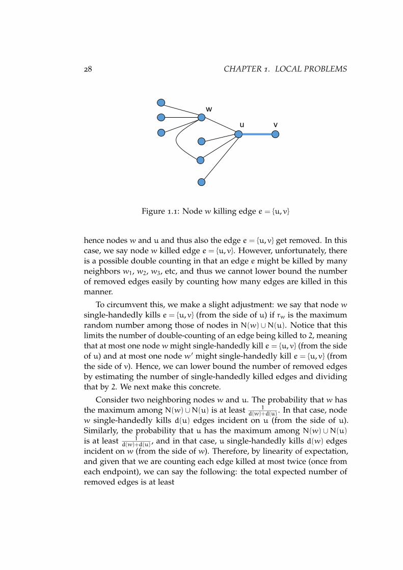
For that, let us consider an edge e = u, v and a neighbor w of u, asdepicted in Figure 1.1. If w has the maximum number among N(w), theset of neighbors of w in the remaining graph, then w joins the MIS and

10One can easily see that having real numbers is unnecessary and values with O(logn)-bit precision suffice.


w

u v

Figure 1.1: Node w killing edge e = u, v

hence nodes w and u and thus also the edge e = u, v get removed. In thiscase, we say node w killed edge e = u, v. However, unfortunately, thereis a possible double counting in that an edge e might be killed by manyneighbors w1, w2, w3, etc, and thus we cannot lower bound the numberof removed edges easily by counting how many edges are killed in thismanner.

To circumvent this, we make a slight adjustment: we say that node wsingle-handedly kills e = u, v (from the side of u) if rw is the maximumrandom number among those of nodes in N(w) ∪N(u). Notice that thislimits the number of double-counting of an edge being killed to 2, meaningthat at most one node w might single-handedly kill e = u, v (from the sideof u) and at most one node w ′ might single-handedly kill e = u, v (fromthe side of v). Hence, we can lower bound the number of removed edgesby estimating the number of single-handedly killed edges and dividingthat by 2. We next make this concrete.

Consider two neighboring nodes w and u. The probability that w hasthe maximum among N(w)∪N(u) is at least 1

d(w)+d(u) . In that case, nodew single-handedly kills d(u) edges incident on u (from the side of u).Similarly, the probability that u has the maximum among N(w) ∪N(u)

is at least 1d(w)+d(u) , and in that case, u single-handedly kills d(w) edges

incident on w (from the side of w). Therefore, by linearity of expectation,and given that we are counting each edge killed at most twice (once fromeach endpoint), we can say the following: the total expected number ofremoved edges is at least

1.7. SUBLOGARITHMIC-TIME RANDOMIZED COLORING 29

E[mi −mi+1] >∑

w,u∈Ei

( d(u)

d(w) + d(u)+

d(w)

d(w) + d(u)

)/2 = mi/2.

1.7 Sublogarithmic-Time Randomized Coloring

Here, we explain a randomized algorithm that achieves the following:

Theorem 1.45. There is a randomized LOCAL algorithm that computes a ∆(1+ε)-coloring in O(

√logn) rounds11, for any constant ε > 0, with high probability.

We present the algorithm in two parts: we first explain the algorithmassuming that ∆ 6 2

√logn, and then we extend the algorithm to larger ∆

using a small additional step.

1.7.1 The algorithm for low-degree graphs

Theorem 1.46. There is a randomized algorithm that computes a ∆(1+ ε) col-oring of the graph in Θ(

√logn/ε) rounds, for any constant ε > 0, assuming12

that ∆ 6 2√

logn.

Suppose that each vertex has degree at most 2√

logn. Consider runningthe following algorithm for Θ(

√logn/ε) iterations. In each iteration, each

node v picks a random color among the colors not previously taken by anyof its neighbors. If no neighbor of v picked the same color, then v takesthis color as its permanent coloring, and gets removed from the problem.The neighbors update their palette of remaining colors, by removing thecolors taken by the colored neighbors.

In Lemma 1.47 below, we show that after Θ(√

logn/ε) iterations forany ε ∈ (0, 1], with high probability, each connected component of theremaining graph has diameter at most Θ(

√logn/ε). Hence, each of these

components can be colored in Θ(√

logn/ε) additional steps, deterministi-cally. Therefore, once we prove Lemma 1.47, we have essentially completedthe proof of Theorem 1.46.

11We remark that a much faster algorithm, with a round complexity of 2O(√

log logn), isknown. We will cover that result in the next sections.

12As mentioned before, we will soon see how to remove this assumption.


Lemma 1.47. After Θ(√

logn/ε) iterations, with high probability, each con-nected component in the subgraph induced by the remaining nodes has at diameterat most Θ(

√logn/ε).

Proof. We show that with high probability, no path of length C√

logn/εcan have all of its vertices remain, for a large enough constant C > 3.

We start with some simple observations. Notice that in every iteration,the palette size of each node is at least a (1 + ε) factor larger than itsnumber of remaining neighbors, i.e., its degree in the remaining graph.Hence, in each iteration, each node gets colored with probability at leastε/(1+ ε) > ε/2, even independent of its neighbors (why?).

Consider an arbitrary path P = v0, v1, . . . , v` where ` = Θ(√

logn/ε). Ineach iteration, each of these vertices gets removed with probability at leastε, regardless of the coloring of the other vertices. Hence, the probabilitythat all these nodes remain for k = C

√logn/ε iterations is at most

(1− ε/2)`k 6 exp(−`kε/2) 6 exp(−C2 logn/(2ε)).

Now, there are at most n∆` ways for choosing the path P, because thereare n choices for the starting point and then ∆ choices for each next hop.Hence, by a union bound, the probability that any such path remains is atmost

n ·∆` · exp(−C logn/(2ε))= exp(logn+ ` log∆−C2 logn/(2ε))

6 exp(logn+C√

logn/ε ·√

logn−C2 logn/(2ε))

= exp(logn+C logn/ε−C2 logn/(2ε)) 6 1/nC.

1.7.2 The extension to high-degree graphs

We now see how to extend Theorem 1.46 to higher degree graphs, usingone extremely simple step.

Theorem 1.48. There is a randomized algorithm that computes a ∆(1+ ε) color-ing of the graph in Θ(

√logn/ε) rounds, for any constant ε > 0.

Suppose that ∆ > 2√

logn, as otherwise Theorem 1.46 suffices. PartitionG into k = αε2∆/ logn vertex-disjoint subgraphs G1, G2, G3, . . . , Gk by

1.7. SUBLOGARITHMIC-TIME RANDOMIZED COLORING 31

putting each vertex in one of these subgraphs at random. Here, α is asufficiently small positive constant α > 0. In Lemma 1.49, we argue that,with high probability, each subgraph has degree at most ∆

k (1 + ε/3) =

O(logn). This will be by a simple application of the Chernoff bound.Hence, it can be colored using ∆

k (1+ ε/3)(1+ ε/3) 6∆k (1+ ε) colors, via the

method of Theorem 1.46, in Θ(√

logn/ε) rounds. We use different colorsfor different subgraphs, and color them all in parallel. Hence, overall, weget a coloring with k · ∆k (1+ ε) = ∆(1+ ε) colors, in Θ(

√logn/ε) rounds.

Lemma 1.49. With high probability, each subgraph Gi has maximum degree atmost ∆k (1+ ε/3).

The lemma follows in a straightforward manner from the Chernoffbound, and a union bound. The Chernoff bound is among the mostbasic concentration of measure tools. In a rough sense, it shows that thesum of independent (indicator) random variables has a distribution well-concentrated around its expected value. More concretely, the probabilitythat this sum deviates significantly from its expected value is exponentiallysmall in the expected value. The mathematical statement is as follows:

Theorem 1.50. (Chernoff Bound) Suppose X1, X2, . . . , Xη are independentrandom variables taking values in 0, 1. Let X =

∑`i=1 Xi denote their sum and

let µ = E[X] denote the sum’s expected value. For any 0 < δ 6 1, we have

Pr[X /∈ [µ(1− δ),µ(1+ δ)] 6 2e−δ2µ/3.

Proof of Lemma 1.49. Consider each node v ∈ G. Let X1, X2, . . .X∆ be theindicator random variables of whether the ith neighbor of v picks the samesubgraph as v does. Let X =

∑`i=1 Xi and µ = E[X]. Notice that µ = ∆/k.

Given that k = αε2∆/ logn, we get that µ > lognαε2

. Hence, by Chernoffbound, we have

Pr[X > µ(1+ ε/3)] 6 2e−ε2µ/18 6 e1−logn/(18α) 6 1/n3,

where the last inequality holds for small enough α, e.g., α = 0.01.Now, we know that the probability of one node v having a degree (in

its own subgraph) higher than the desired threshold ∆(1+ε/3)k is at most

1/n3. By a union bound over all nodes v, we get that the probability ofhaving such a node is at most 1/n2. In other words, with high probability,each node has degree at most ∆(1+ε/3)k in its own subgraph.


1.8 Exercises

Exercise 1.1. In Lemma 1.5, we saw a single-round algorithm for reducing thenumber of colors exponentially. Here, we discuss another such method, whichtransforms any k-coloring of any rooted-tree to a 2 logk-coloring, so long ask > C0 for a constant C0.

The method works as follows. Let each node u send its color φold(u) to itschildren. Now, each node v computes its new color φnew(v) as follows: Considerthe binary representation of φold(v) and φold(u), where u is the parent of v.Notice that each of these is a log2 k-bit value. Let iv be the smallest index i suchthat the binary representations of φold(v) and φold(u) differ in the ith bit. Letbv be the ithv bit of φold(v). Define φnew(v) = (iv,bv). Prove that φold(v) iswell-defined, and that it is a proper (2 logk)-coloring.

Exercise 1.2. Here, we use the concept of cover free families, as defined inDefinition 1.17, to obtain an encoding that allows us to recover information aftersuperimposition. That is, we will be able to decode even if k of the codewords aresuperimposed and we only have the resulting bit-wise OR.

More concretely, we want a function Enc : 0, 1logn → 0, 1m — that encodesn possibilities using m-bit strings for m > log2n — such that the followingproperty is satisfied: ∀S,S ′ ⊆ 1, ...,n such that |S| 6 k and |S ′| 6 k, we havethat ∨i∈SEnc(i) 6= ∨i∈S ′Enc(i). Here ∨ denotes the bit-wise OR operation.

Present such an encoding function, with a small m, that depends on n and k.What is the best m that you can achieve?

Exercise 1.3. This exercise has two parts:

(A) Design a single-round algorithm that transforms any given k-coloring ofa graph with maximum degree ∆ into a k ′-coloring for k ′ = k− d k

2(∆+1)e,assuming k ′ > ∆+ 1.

(B) Use repetitions of this single-round algorithm, in combination with theO(log∗ n)-roundO(∆2)-coloring of Theorem 1.16, to obtain anO(∆ log∆+

log∗ n)-round (∆+ 1)-coloring algorithm.

Exercise 1.4. Here, we see yet another deterministic method for computing a(∆ + 1)-coloring in O(∆ log∆ + log∗ n) rounds. First, using Theorem 1.16,we compute an O(∆2)-coloring φold in O(log∗ n) rounds. What remains is totransform this into a (∆+ 1)-coloring, in O(∆ log∆) additional rounds.

The current O(∆2)-coloring φold can be written using C log∆ bits, assuminga sufficiently large constant C. This bit complexity will be the parameter of our

1.8. EXERCISES 33

recursion. Partition G into two vertex-disjoint subgraphs G0 and G1, based onthe most significant bit in the color φold. Notice that each of G0 and G1 inherits acoloring with C log∆− 1 bits. Solve the ∆+ 1 coloring problem in each of theseindependently and recursively. Then, we need to merge these colors, into a ∆+ 1

coloring for the whole graph.

(A) Explain an O(∆)-round algorithm, as well its correctness proof, that oncethe independent (∆+ 1)-colorings of G0 and G1 are finished, updates onlythe colors of G1 vertices to ensure that the overall coloring is a proper(∆+ 1)-coloring of G = G0 ∪G1.

(B) Provide a recursive time-complexity analysis that proves that overall, therecursive method takes O(∆ log∆) rounds.

Exercise 1.5. Explain how given a (C,D) network decomposition of graph G, amaximal independent set can be computed in O(CD) rounds.

Exercise 1.6. Prove Lemma 1.32.

Exercise 1.7. Improve the round complexity of the algorithm stated in Theo-rem 1.31 to O(logn) rounds.

Exercise 1.8. We here see that the network decomposition obtained in Theo-rem 1.31 has the nearly best possible parameters. In particular, it is known thatthere are n-node graphs that have girth13 Ω(logn/ log logn) and chromaticnumber Ω(logn)[AS04, Erd59]. Use this fact to argue that on these graphs, an(o(logn),o(logn/ log logn)) network decomposition does not exist.

Exercise 1.9. Given an n-node undirected graph G = (V ,E), a d(n)-diameterordering of G is a one-to-one labeling f : V → 1, 2, . . . ,n of vertices such that forany path P = v1, v2, . . . , vp on which the labels f(vi) are monotonically increasing,any two nodes vi, vj ∈ P have distG(vi, vj) 6 d(n).

Use the network decomposition of Theorem 1.31 to argue that each n-nodegraph has an O(log2 n)-diameter ordering.

Exercise 1.10. Consider the following simple 1-round randomized algorithm:each node v picks a random real number rv ∈ [0, 1] and then, v joins a set S ifits random number is a local minima, that is, if rv < ru for all neighbors u of v.Prove that, with high probability, the set S is a (2,O(logn))-ruling set.

13Recall that the girth of a graph is the length of its shortest cycle.

Bibliography

[ABI86] Noga Alon, László Babai, and Alon Itai. A fast and simplerandomized parallel algorithm for the maximal independentset problem. Journal of algorithms, 7(4):567–583, 1986.

[ALGP89] Baruch Awerbuch, M Luby, AV Goldberg, and Serge A Plotkin.Network decomposition and locality in distributed computa-tion. In Foundations of Computer Science, 1989., 30th AnnualSymposium on, pages 364–369. IEEE, 1989.

[AS04] Noga Alon and Joel H Spencer. The probabilistic method. JohnWiley & Sons, 2004.

[Bar15] Leonid Barenboim. Deterministic (δ+ 1)-coloring in sublinear(in δ) time in static, dynamic and faulty networks. In Pro-ceedings of the 2015 ACM Symposium on Principles of DistributedComputing, pages 345–354. ACM, 2015.

[Bol78] Béla Bollobás. Chromatic number, girth and maximal degree.Discrete Mathematics, 24(3):311–314, 1978.

[CFS10] David Conlon, Jacob Fox, and Benny Sudakov. Hypergraphramsey numbers. Journal of the American Mathematical Society,23(1):247–266, 2010.

[CLRS01] Thomas H.. Cormen, Charles Eric Leiserson, Ronald L Rivest,and Clifford Stein. Introduction to algorithms, volume 6. MITpress Cambridge, 2001.

[CV86] Richard Cole and Uzi Vishkin. Deterministic coin tossingand accelerating cascades: micro and macro techniques fordesigning parallel algorithms. In Proceedings of the eighteenthannual ACM symposium on Theory of computing, pages 206–219.ACM, 1986.

35

36 BIBLIOGRAPHY

[Erd59] Paul Erdos. Graph theory and probability. Canada J. Math,11:34G38, 1959.

[FHK16] Pierre Fraigniaud, Marc Heinrich, and Adrian Kosowski. Localconflict coloring. In Proc. of the Symp. on Found. of Comp. Sci.(FOCS), 2016.

[GPS87] Andrew Goldberg, Serge Plotkin, and Gregory Shannon. Paral-lel symmetry-breaking in sparse graphs. In Proceedings of thenineteenth annual ACM symposium on Theory of computing, pages315–324. ACM, 1987.

[Jam11] Mohammad Shoaib Jamall. A brooks’ theorem for triangle-freegraphs. arXiv preprint arXiv:1106.1958, 2011.

[Kim95] Jeong Han Kim. On brooks’ theorem for sparse graphs. Combi-natorics, Probability and Computing, 4(02):97–132, 1995.

[Kuh09] Fabian Kuhn. Weak graph colorings: distributed algorithmsand applications. In Proceedings of the twenty-first annual sympo-sium on Parallelism in algorithms and architectures, pages 138–144.ACM, 2009.

[KW06] Fabian Kuhn and Rogert Wattenhofer. On the complexity ofdistributed graph coloring. In Proceedings of the twenty-fifthannual ACM symposium on Principles of distributed computing,pages 7–15. ACM, 2006.

[Lin87] Nathan Linial. Distributive graph algorithms global solutionsfrom local data. In Proc. of the Symp. on Found. of Comp. Sci.(FOCS), pages 331–335. IEEE, 1987.

[Lin92] Nathan Linial. Locality in distributed graph algorithms. SIAMJournal on Computing, 21(1):193–201, 1992.

[LS91] Nathan Linial and Michael Saks. Decomposing graphs intoregions of small diameter. In Proceedings of the Second AnnualACM-SIAM Symposium on Discrete Algorithms, SODA ’91, pages320–330, 1991.

[LS14] Juhana Laurinharju and Jukka Suomela. Brief announcement:Linial’s lower bound made easy. In Proceedings of the 2014 ACM

BIBLIOGRAPHY 37

symposium on Principles of distributed computing, pages 377–378.ACM, 2014.

[Lub66] David Lubell. A short proof of sperner’s lemma. Journal ofCombinatorial Theory, 1(2):299, 1966.

[Lub85] Michael Luby. A simple parallel algorithm for the maximalindependent set problem. In Proc. of the Symp. on Theory ofComp. (STOC), pages 1–10, 1985.

[Nao91] Moni Naor. A lower bound on probabilistic algorithms fordistributive ring coloring. SIAM Journal on Discrete Mathematics,4(3):409–412, 1991.

[NS93] Moni Naor and Larry Stockmeyer. What can be computedlocally? In Proceedings of the twenty-fifth annual ACM symposiumon Theory of computing, pages 184–193. ACM, 1993.

[NS95] Moni Naor and Larry Stockmeyer. What can be computedlocally? SIAM Journal on Computing, 24(6):1259–1277, 1995.

[PS92] Alessandro Panconesi and Aravind Srinivasan. Improved dis-tributed algorithms for coloring and network decompositionproblems. In Proc. of the Symp. on Theory of Comp. (STOC), pages581–592. ACM, 1992.

[PS15] Seth Pettie and Hsin-Hao Su. Distributed coloring algorithmsfor triangle-free graphs. Information and Computation, 243:263–280, 2015.

[RS14] Joel Rybicki and Jukka Suomela. Exact bounds for distributedgraph colouring. In International Colloquium on Structural In-formation and Communication Complexity, pages 46–60. Springer,2014.

[Spe28] Emanuel Sperner. Ein satz über untermengen einer endlichenmenge. Mathematische Zeitschrift, 27(1):544–548, 1928.

[SV93] Márió Szegedy and Sundar Vishwanathan. Locality basedgraph coloring. In Proceedings of the twenty-fifth annual ACMsymposium on Theory of computing, pages 201–207. ACM, 1993.

38 BIBLIOGRAPHY

[Edm65] Jack Edmonds. Maximum matching and a polyhedron with 0,1-vertices. Journal of Research of the National Bureau of StandardsB, 69(125-130):55–56, 1965.

[MR10] Rajeev Motwani and Prabhakar Raghavan. Randomized algo-rithms. Chapman & Hall/CRC, 2010.

[NO08] Huy N Nguyen and Krzysztof Onak. Constant-time approx-imation algorithms via local improvements. In Foundations ofComputer Science. FOCS’08. IEEE 49th Annual IEEE Symposiumon, pages 327–336. IEEE, 2008.

computer science, eth zurichcomputer science, eth zurich mohsen ghaffari march 2019. ii. contents...

Documents