ComputerVision

Fitting

Marc PollefeysCOMP 256

Some slides and illustrations from D. Forsyth, T. Darrel, A. Zisserman, ...

ComputerVision

2

Jan 16/18 - Introduction

Jan 23/25 Cameras Radiometry

Jan 30/Feb1 Sources & Shadows Color

Feb 6/8 Linear filters & edges Texture

Feb 13/15 Multi-View Geometry Stereo

Feb 20/22 Optical flow Project proposals

Feb27/Mar1 Affine SfM Projective SfM

Mar 6/8 Camera Calibration Segmentation

Mar 13/15 Springbreak Springbreak

Mar 20/22 Fitting Prob. Segmentation

Mar 27/29 Silhouettes and Photoconsistency

Linear tracking

Apr 3/5 Project Update Non-linear Tracking

Apr 10/12 Object Recognition Object Recognition

Apr 17/19 Range data Range data

Apr 24/26 Final project Final project

Tentative class schedule

ComputerVision

3

Last time: Segmentation

• Group tokens into clusters that fit together– foreground-background

– cluster on intensity, color, texture, location, …• K-means

• graph-based

ComputerVision

4

Fitting

• Choose a parametric object/some objects to represent a set of tokens

• Most interesting case is when criterion is not local– can’t tell whether a

set of points lies on a line by looking only at each point and the next.

• Three main questions:– what object

represents this set of tokens best?

– which of several objects gets which token?

– how many objects are there?

(you could read line for object here, or circle, or ellipse or...)

ComputerVision

5

Hough transform : straight lines

implementation :

1. the parameter space is discretised2. a counter is incremented at each cell where the lines pass 3. peaks are detected

yaxb )(

ComputerVision

6

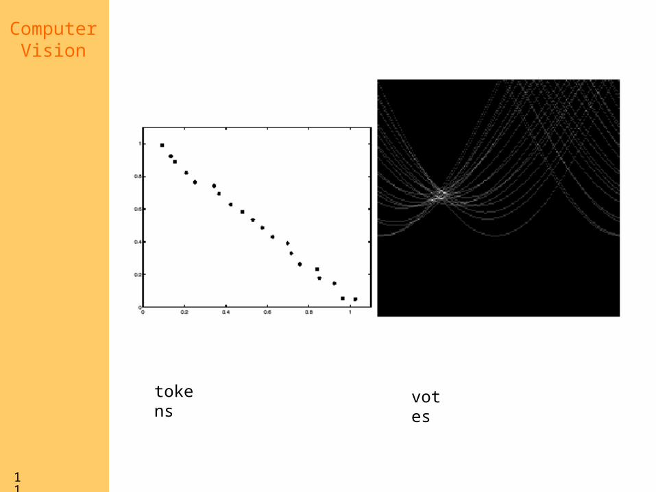
Hough transform : straight linesproblem : unbounded parameter domain vertical lines require infinite a

sincos yx

Each point will add a cosine function in the (,) parameter space

alternative representation:

ComputerVision

7

tokensvotes

ComputerVision

8

Hough transform : straight lines

Square : Circle :

ComputerVision

9

Hough transform : straight lines

ComputerVision

10

Mechanics of the Hough transform

• Construct an array representing , d

• For each point, render the curve (, d) into this array, adding one at each cell

• Difficulties– how big should the

cells be? (too big, and we cannot distinguish between quite different lines; too small, and noise causes lines to be missed)

• How many lines?– count the peaks in the

Hough array

• Who belongs to which line?– tag the votes

• Hardly ever satisfactory in practice, because problems with noise and cell size defeat it

ComputerVision

11

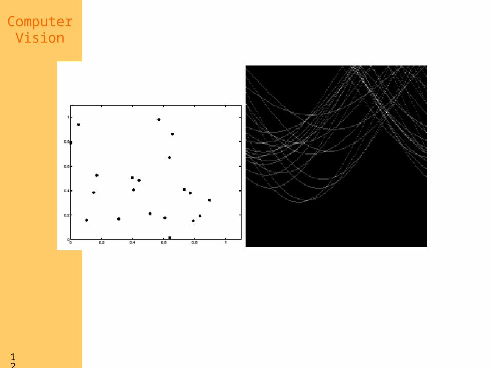
tokens votes

ComputerVision

12

ComputerVision

13

ComputerVision

14

ComputerVision

15

Cascaded hough transformTuytelaars and Van Gool ICCV‘98

ComputerVision

16

Line fitting can be max.likelihood - but choice ofmodel is important

standard least-squares

total least-squares

ComputerVision

17

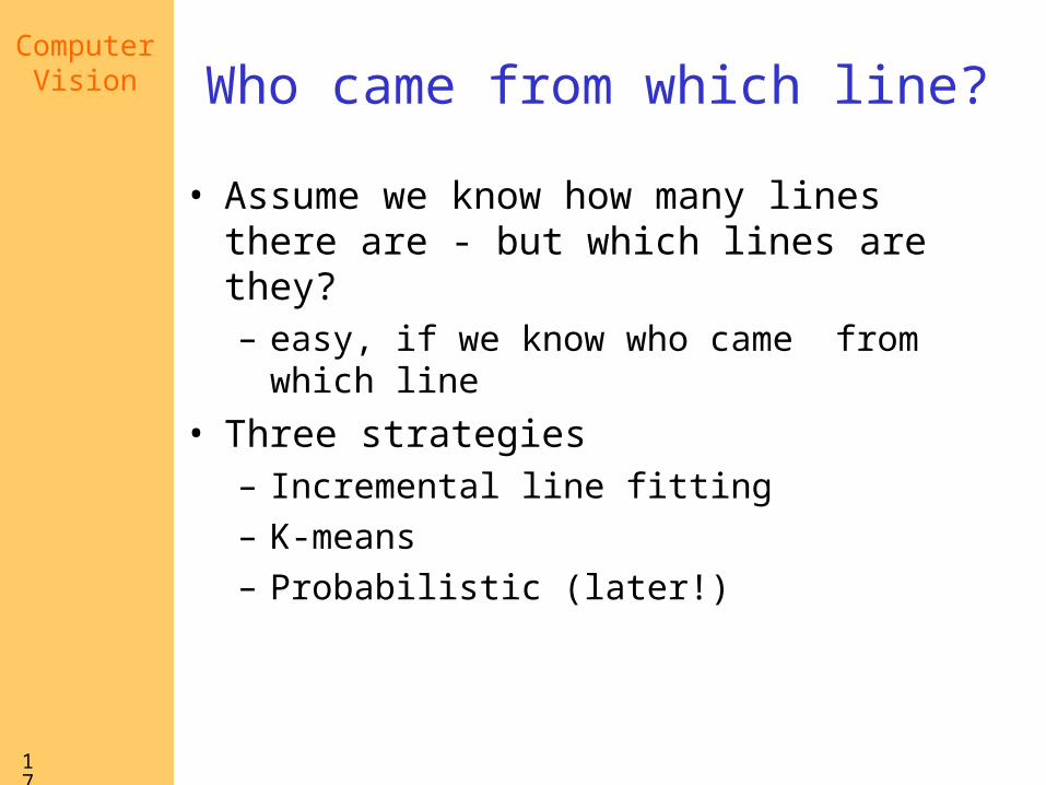
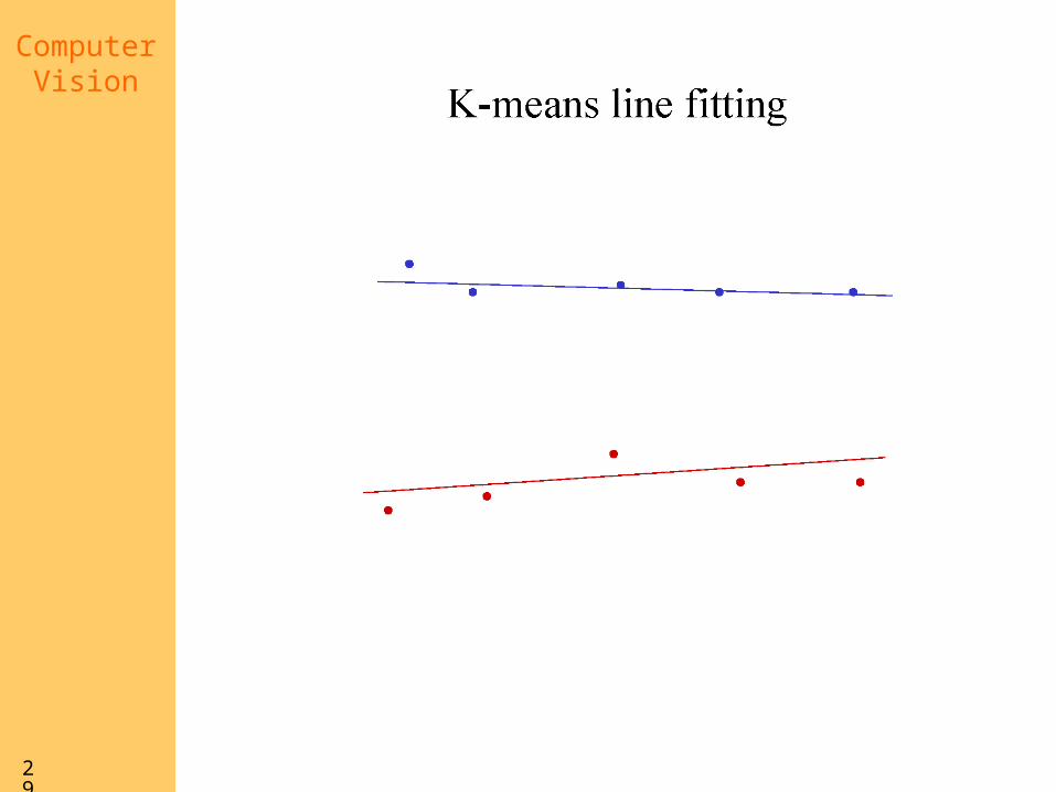
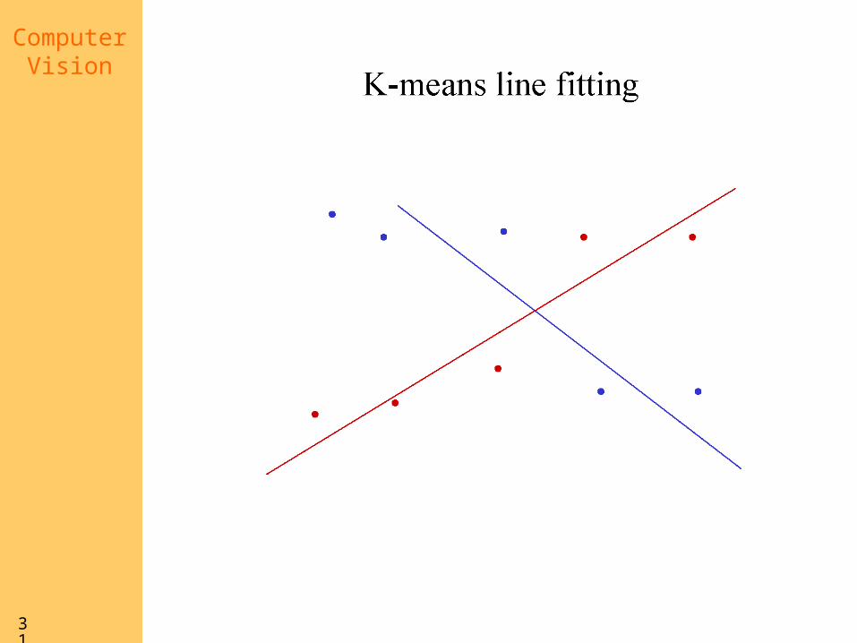
Who came from which line?

• Assume we know how many lines there are - but which lines are they?– easy, if we know who came from which

line

• Three strategies– Incremental line fitting– K-means– Probabilistic (later!)

ComputerVision

18

ComputerVision

19

ComputerVision

20

ComputerVision

21

ComputerVision

22

ComputerVision

23

ComputerVision

24

ComputerVision

25

ComputerVision

26

ComputerVision

27

ComputerVision

28

ComputerVision

29

ComputerVision

30

ComputerVision

31

ComputerVision

32

Robustness

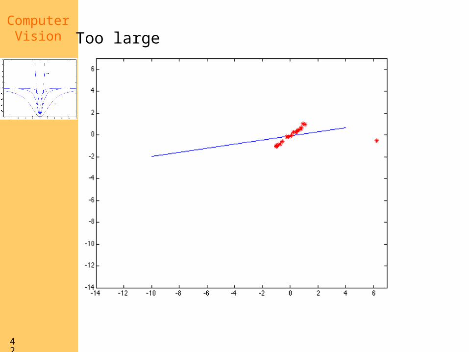
• As we have seen, squared error can be a source of bias in the presence of noise points– One fix is EM - we’ll do this shortly– Another is an M-estimator

• Square nearby, threshold far away

– A third is RANSAC• Search for good points

ComputerVision

33

ComputerVision

34

ComputerVision

35

ComputerVision

36

ComputerVision

37

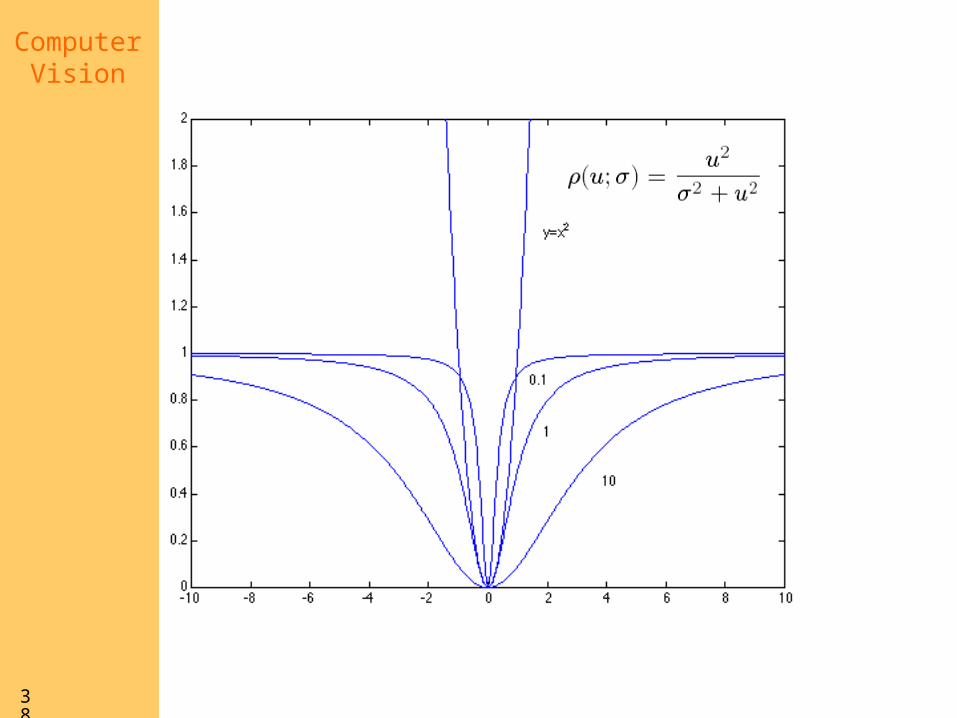
M-estimators

• Generally, minimize

where is the residual

;,iii

xr

,ii xr

ComputerVision

38

ComputerVision

39

ComputerVision

40

ComputerVision

41

Too small

ComputerVision

42

Too large

ComputerVision

43

ComputerVision

44

RANSAC

• Choose a small subset uniformly at random

• Fit to that• Anything that is close

to result is signal; all others are noise

• Refit• Do this many times

and choose the best

• Issues– How many times?

• Often enough that we are likely to have a good line

– How big a subset?• Smallest possible

– What does close mean?• Depends on the

problem

– What is a good line?• One where the number

of nearby points is so big it is unlikely to be all outliers

ComputerVision

45

ComputerVision

46

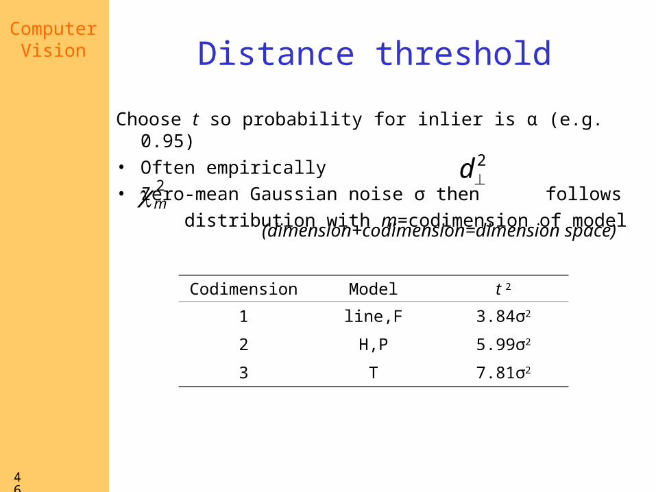
Distance threshold

Choose t so probability for inlier is α (e.g. 0.95) • Often empirically• Zero-mean Gaussian noise σ then follows

distribution with m=codimension of model

2d2

m(dimension+codimension=dimension space)

Codimension Model t 2

1 line,F 3.84σ2

2 H,P 5.99σ2

3 T 7.81σ2

ComputerVision

47

How many samples?

Choose N so that, with probability p, at least one random sample is free from outliers. e.g. p=0.99

sepN 11log/1log

peNs 111

proportion of outliers e

s 5% 10% 20% 25% 30% 40% 50%2 2 3 5 6 7 11 173 3 4 7 9 11 19 354 3 5 9 13 17 34 725 4 6 12 17 26 57 1466 4 7 16 24 37 97 2937 4 8 20 33 54 163 5888 5 9 26 44 78 272 1177

ComputerVision

48

Acceptable consensus set?

• Typically, terminate when inlier ratio reaches expected ratio of inliers

neT 1

ComputerVision

49

Adaptively determining the number of samples

e is often unknown a priori, so pick worst case, e.g. 50%, and adapt if more inliers are found, e.g. 80% would yield e=0.2

– N=∞, sample_count =0– While N >sample_count repeat

• Choose a sample and count the number of inliers• Set e=1-(number of inliers)/(total number of points)• Recompute N from e• Increment the sample_count by 1

– Terminate

sepN 11log/1log

ComputerVision

50

Step 1. Extract featuresStep 2. Compute a set of potential matchesStep 3. do

Step 3.1 select minimal sample (i.e. 7 matches)

Step 3.2 compute solution(s) for F

Step 3.3 determine inliers

until (#inliers,#samples)<95%

samples#7)1(1

matches#inliers#

#inliers 90% 80% 70% 60% 50%

#samples 5 13 35 106 382

Step 4. Compute F based on all inliersStep 5. Look for additional matchesStep 6. Refine F based on all correct matches

(generate hypothesis)

(verify hypothesis)

RANSAC for Fundamental Matrix

ComputerVision

51

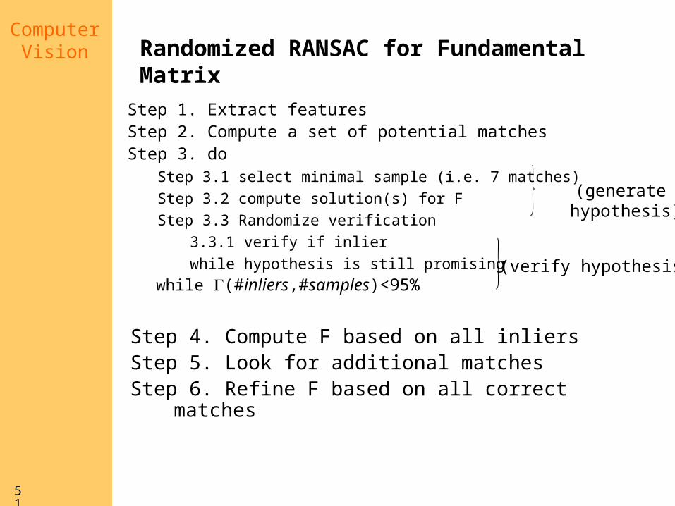
Step 1. Extract featuresStep 2. Compute a set of potential matchesStep 3. do

Step 3.1 select minimal sample (i.e. 7 matches)

Step 3.2 compute solution(s) for F

Step 3.3 Randomize verification

3.3.1 verify if inlier

while hypothesis is still promising

while (#inliers,#samples)<95%

Step 4. Compute F based on all inliersStep 5. Look for additional matchesStep 6. Refine F based on all correct matches

(generate hypothesis)

(verify hypothesis)

Randomized RANSAC for Fundamental Matrix

ComputerVision

52

Example: robust computation

Interest points(500/image)(640x480)

Putative correspondences (268)(Best match,SSD<20,±320)

Outliers (117)(t=1.25 pixel; 43 iterations)

Inliers (151)

Final inliers (262)(2 MLE-inlier cycles; d=0.23→d=0.19; IterLev-Mar=10)

#in 1-e adapt. N

6 2% 20M

10 3% 2.5M

44 16% 6,922

58 21% 2,291

73 26% 911

151 56% 43

from H&Z

ComputerVision

53

More on robust estimation

• LMedS, an alternative to RANSAC(minimize Median residual in stead of maximizing inlier count)

• Enhancements to RANSAC– Randomized RANSAC– Sample ‘good’ matches more frequently– …

• RANSAC is also somewhat robust to bugs, sometimes it just takes a bit longer…

ComputerVision

54

RANSAC for quasi-degenerate data

• Often data can be almost degeneratee.g. 337 matches on plane, 11 off plane

• RANSAC gets confused by quasi-degenerate data

Probability of valid non-degenerate sample

Probability of success for RANSAC (aiming for 99%)

planar points only provide 6 in stead of 8 linearly independent equations for F

ComputerVision

55

RANSAC for quasi-degenerate data(QDEGSAC) (Frahm and Pollefeys, CVPR06)

QDEGSAC estimates robust rank of datamatrix (i.e. large % of rows approx. fit in a lower dimensional subspace)

ComputerVision

56

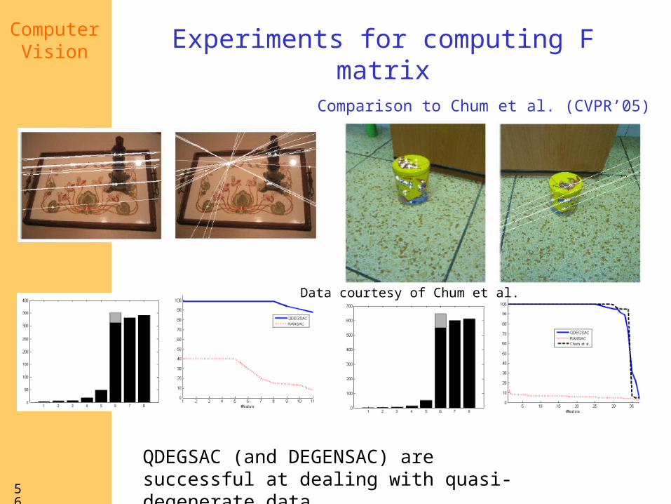
Experiments for computing F matrix

Comparison to Chum et al. (CVPR’05)

Data courtesy of Chum et al.

QDEGSAC (and DEGENSAC) are successful at dealing with quasi-degenerate data

ComputerVision

57

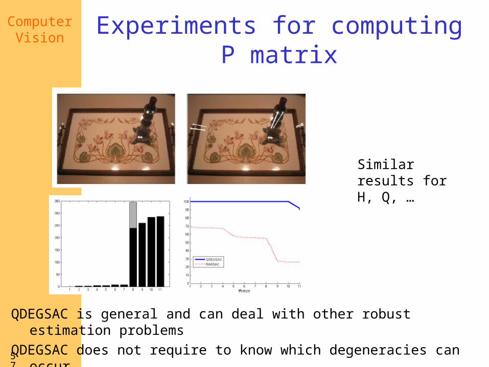
Experiments for computing P matrix

QDEGSAC is general and can deal with other robust estimation problems

QDEGSAC does not require to know which degeneracies can occur

Similar results for H, Q, …

ComputerVision

58

Fitting curves other than lines

• In principle, an easy generalisation– The probability of

obtaining a point, given a curve, is given by a negative exponential of distance squared

• In practice, rather hard– It is generally

difficult to compute the distance between a point and a curve

ComputerVision

59

Next class: Segmentation and Fitting using Probabilistic Methods

Reading: Chapter 16

Missing data: EM algorithm

Model selection