computerised measurement of contact angles

1

Eugen G. Leuze Verlag 108 Jahre

Galvanotechnik

Galvanotechnik 10/2010

1 Introduction

The measurement of the contact angle formed by a droplet of liquid placed on a horizontal surface – the so-called sessile drop – has been of interest to scientists and others for at least 200 years, since Young first reported his observations [1]. From this parameter, much valuable information can be calcu-lated, notably surface energy values. These in turn can provide information on surface contamination or the wettability of a surface [2]. For this reason, the measurement of contact angles is of importance in a wide range of scientific and technological fields, including medicine, surface science, surface engi-neering, and industries producing inks and coatings for plastics and textile goods as described by Adam-son [3], Hansen [4], Zisman, and coworkers [5].The earliest measurements, such as that of Young, used a protractor or a similar graduated scale for measuring the angle. Various other techniques were developed, such as the so-called half-angle method, discussed below. The assumption that the sessile drop was spherical, or formed part of a sphere, underpinned the basis of these methods wherein the contact angle values were computed using the principles of Euclid-ian geometry.The two most widely-used such methods were:– Constructing a tangent by drawing a line orthogo-

nal to the drop radius that intersects the point of contact with the horizontal surface – the triphase point;

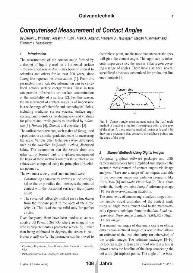
– The so-called half-angle method uses a line drawn from the triphase point to the apex of the circle (Fig. 1). This is of course valid only for perfect circles.

Over the years, there have been modest advances, notably US Patent 5,268,733 where an image of the drop is projected onto a protractor screen [6]. Rather than being calibrated in degrees, the screen is cali-brated at half-scale. The protractor can be moved to

the triphase point, and the trace that intersects the apex will give the contact angle. This approach is inher-ently imprecise since the apex is a flat region cover-ing a range of angles. There have also been several specialized advances customized for production-line environments [7].

ComputerisedMeasurementofContactAnglesBy Darren L. Williamsa, Anselm T. Kuhnb, Mark A. Amanna, Madison B. Hausingera, Megan M. Konarika and Elizabeth I. Nesselrodea

a Chemistry Department, Sam Houston State University, Huntsville, USA

b Publication service Ltd., Stevenage Herts, Great Britain

Fig. 1: Contact angle measurement using the half-angle method of drawing a line from the triphase point to the apex of the drop. A more precise method measures b and h by drawing a rectangle that connects the triphase points and the apex of the drop

2 ManualMethodsUsingDigitalImages

Computer graphics software packages and USB camera microscopes have simplified and improved the accurate measurement of contact angles via image analysis. There are a range of techniques available in the common image manipulation programs like CorelDraw [8] and Adobe Photoshop [9]. The authors prefer the freely-available ImageJ software package [10] for its ever-expanding flexibility. The complexity of contact angle analysis ranges from the simple visual estimation of the contact angle using an angle measurement tool to the mathemati-cally rigorous technique found in the Low-Bond Axi-symmetric Drop Shape Analysis (LBADSA) Plugin [11] for ImageJ. The manual technique of drawing a circle or ellipse onto a cross-sectional image of a sessile drop allows an estimate of the true circularity (or otherwise) of the droplet image. The software packages [8–10] include an angle measurement tool wherein a line is drawn across the baseline of the drop connecting the left and right triphase points. The angle of the base-

2

Eugen G. Leuze Verlag108 Jahre

Galvanotechnik


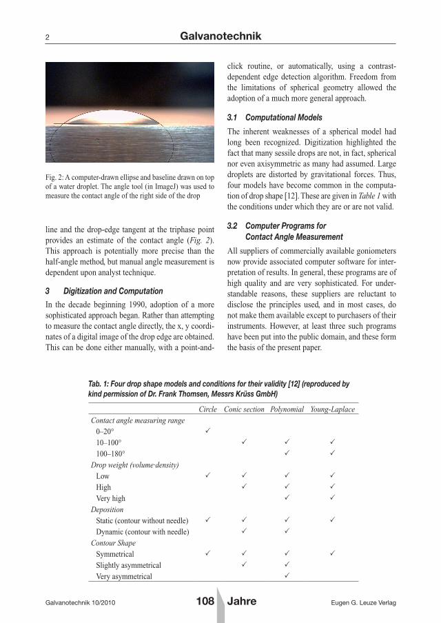
line and the drop-edge tangent at the triphase point provides an estimate of the contact angle (Fig. 2). This approach is potentially more precise than the half-angle method, but manual angle measurement is dependent upon analyst technique.

3 DigitizationandComputation

In the decade beginning 1990, adoption of a more sophisticated approach began. Rather than attempting to measure the contact angle directly, the x, y coordi-nates of a digital image of the drop edge are obtained. This can be done either manually, with a point-and-

click routine, or automatically, using a contrast-dependent edge detection algorithm. Freedom from the limitations of spherical geometry allowed the adoption of a much more general approach.

3.1 ComputationalModels

The inherent weaknesses of a spherical model had long been recognized. Digitization highlighted the fact that many sessile drops are not, in fact, spherical nor even axisymmetric as many had assumed. Large droplets are distorted by gravitational forces. Thus, four models have become common in the computa-tion of drop shape [12]. These are given in Table 1 with the conditions under which they are or are not valid.

3.2 ComputerProgramsforContactAngleMeasurement

All suppliers of commercially available goniometers now provide associated computer software for inter-pretation of results. In general, these programs are of high quality and are very sophisticated. For under-standable reasons, these suppliers are reluctant to disclose the principles used, and in most cases, do not make them available except to purchasers of their instruments. However, at least three such programs have been put into the public domain, and these form the basis of the present paper.

Tab.1:Fourdropshapemodelsandconditionsfortheirvalidity[12](reproducedbykindpermissionofDr.FrankThomsen,MessrsKrüssGmbH)

Circle Conic section Polynomial Young-LaplaceContact angle measuring range

0–20°

10–100°

100–180°

Drop weight (volume·density)Low

High

Very high

DepositionStatic (contour without needle)

Dynamic (contour with needle)

Contour ShapeSymmetrical

Slightly asymmetrical

Very asymmetrical

Fig. 2: A computer-drawn ellipse and baseline drawn on top of a water droplet. The angle tool (in ImageJ) was used to measure the contact angle of the right side of the drop

3


Galvanotechnik


3.3 Open-AccessContactAngleComputerPrograms

The three open-access programs of which the authors are aware are all plugins for the ImageJ program. The plugins include the Contact Angle Analysis routine by Brugnara [13], the Low Bond Axisymmetric Drop Shape Analysis (LB-ADSA) technique by Sage et. al. [11], and the DropSnake method by Sage et. al. [14]. Brugnara’s routine supplies the circular and conical-section models in Table 1. The DropSnake routine is an implementation of the polynomial approach in Table 1, and the LB-ADSA plugin uses the Young-Laplace analysis (column 4 in Table 1).

4 Experimental

The purpose of this work was to compare the three plugins noted above by measuring the contact angles present in a common set of digital images. In order to eliminate the many additional variables and errors arising when liquid drops are used, the work was car-ried out using simulated drops, as described below. The drops used in this work were actually spheri-cal lenses of known dimension. Three contact angle conditions (acute, near-normal, and obtuse) were selected to assess the software under a wide range of conditions found in practice.

4.1 StandardSamples

A spherical ruby ball lens (Edmund Optics, NT43-830) with a well-defined diameter (d = 6.000 ± 0.003 mm) was placed in the 13/64 inch hole of a metallic drill gage card (Grainger, 5C732) for the obtuse contact angle standard. A sapphire half-ball lens (Edmund Optics, NT49-556) was placed on a metal surface as

the near-normal contact angle standard. For the acute contact angle standard, the ruby ball was placed in the 15/64 inch hole of the gage card, and the portion of the ball protruding through the other side of the card was photographed.

The high sphericity of the ball lenses allowed us to use the half-angle method (Eq. <1>) with variables defined in Figure 1 to calculate the theoretical con-tact angle (CA) of these samples. In all three cases, a rectangle was drawn on the magnified image so that the base width (b) and drop height (h) could be deter-mined with an uncertainty of ±1 pixel.

CA = 2θ = 2tan-a(2h/b) <1>

These dimensionally-stable elements provided a useful standard for refining the digital imaging tech-niques and for comparing the accuracy of the three contact angle plugins.

4.2 ImagingApparatus

The image capture apparatus consisted of a light source, a collimating mask, an adjustable stage, and a USB microscope. The light source was a 60-W incandescent light in a metal shroud (ACE Hardware, Clamp Lamp) powered by a variable AC power supply (Staco, 3PN1010) for brightness control. The horizontal optical axis was approximately 16 cm above the laser table. The collimating mask consisted of an arch-shaped hole in a 8.5 x 11-inch piece of fiberboard (inset of Fig. 3). The mask was placed between the light source and the stage with the center of the sample stage approximately 10 cm from the collimating mask. The sample stage (DinoLite, MS15X-XY-R) was adjustable horizontally in the X and Y directions with a rotary platform on which

Fig. 3: Apparatus for capturing a high-contrast image of a sessile drop

chm_dlw

Typewritten Text

= 2arctan(2h/b)

chm_dlw

Cross-Out

4


Galvanotechnik


the sample is placed. The microscope (DinoLite, AM411T) was mounted on an adjustable microscope mount (Edmund Optics, NT54-794) supported by a ¾ inch post.

4.3 ImageCaptureSettings

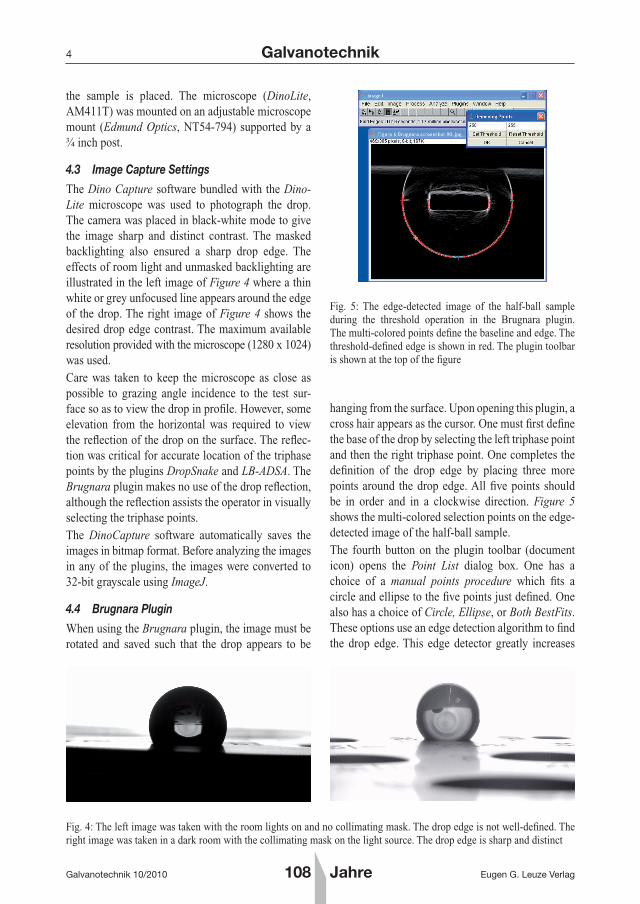
The Dino Capture software bundled with the Dino-Lite microscope was used to photograph the drop. The camera was placed in black-white mode to give the image sharp and distinct contrast. The masked backlighting also ensured a sharp drop edge. The effects of room light and unmasked backlighting are illustrated in the left image of Figure 4 where a thin white or grey unfocused line appears around the edge of the drop. The right image of Figure 4 shows the desired drop edge contrast. The maximum available resolution provided with the microscope (1280 x 1024) was used.Care was taken to keep the microscope as close as possible to grazing angle incidence to the test sur-face so as to view the drop in profile. However, some elevation from the horizontal was required to view the reflection of the drop on the surface. The reflec-tion was critical for accurate location of the triphase points by the plugins DropSnake and LB-ADSA. The Brugnara plugin makes no use of the drop reflection, although the reflection assists the operator in visually selecting the triphase points. The DinoCapture software automatically saves theimages in bitmap format. Before analyzing the images in any of the plugins, the images were converted to 32-bit grayscale using ImageJ.

4.4 BrugnaraPlugin

When using the Brugnara plugin, the image must be rotated and saved such that the drop appears to be

hanging from the surface. Upon opening this plugin, a cross hair appears as the cursor. One must first define the base of the drop by selecting the left triphase point and then the right triphase point. One completes the definition of the drop edge by placing three more points around the drop edge. All five points should be in order and in a clockwise direction. Figure 5 shows the multi-colored selection points on the edge-detected image of the half-ball sample. The fourth button on the plugin toolbar (document icon) opens the Point List dialog box. One has a choice of a manual points procedure which fits a circle and ellipse to the five points just defined. One also has a choice of Circle, Ellipse, or Both BestFits. These options use an edge detection algorithm to find the drop edge. This edge detector greatly increases

Fig. 4: The left image was taken with the room lights on and no collimating mask. The drop edge is not well-defined. The right image was taken in a dark room with the collimating mask on the light source. The drop edge is sharp and distinct

Fig. 5: The edge-detected image of the half-ball sample during the threshold operation in the Brugnara plugin. The multi-colored points define the baseline and edge. The threshold-defined edge is shown in red. The plugin toolbar is shown at the top of the figure

5


Galvanotechnik


the number of points used to define the circle or ellipse.This work used the Both BestFits procedure which automatically detects the drop profile using the edge detection algorithm included in ImageJ. The edge detection algorithm uses a first derivative function of image intensity and a process known as Canny-Deriche Filtering [15]. A highlighted edge image is displayed with a Removing Points dialog box as seen in Figure 5. One should adjust the minimum and maximum threshold values (from 0 to 255) so that the most precise (thin) definition of the edge of the drop is obtained. The Set Threshold button updates the edge image using the new threshold values. Once the settings are accepted, a results window gives the circle contact angle (θ C), left, right, and average contact angle of the ellipse (θ E) in a format that is amenable to copying and pasting into a spreadsheet program. This report window can also be saved as a text file. The Manual Points procedure is very robust in that it will work with any image contrast. However, it depends completely upon the accuracy of point place-

ment by the user. No edge detection or optimization routines are used for this procedure.

4.5 DropSnakePlugin

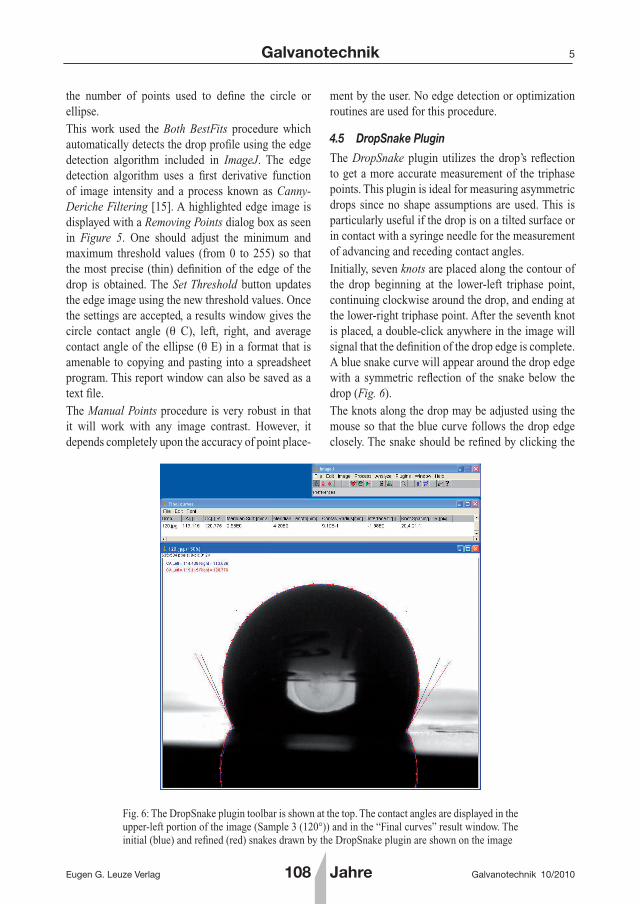
The DropSnake plugin utilizes the drop’s reflection to get a more accurate measurement of the triphase points. This plugin is ideal for measuring asymmetric drops since no shape assumptions are used. This is particularly useful if the drop is on a tilted surface or in contact with a syringe needle for the measurement of advancing and receding contact angles.Initially, seven knots are placed along the contour of the drop beginning at the lower-left triphase point, continuing clockwise around the drop, and ending at the lower-right triphase point. After the seventh knot is placed, a double-click anywhere in the image will signal that the definition of the drop edge is complete. A blue snake curve will appear around the drop edge with a symmetric reflection of the snake below the drop (Fig. 6).The knots along the drop may be adjusted using the mouse so that the blue curve follows the drop edge closely. The snake should be refined by clicking the

Fig. 6: The DropSnake plugin toolbar is shown at the top. The contact angles are displayed in the upper-left portion of the image (Sample 3 (120°)) and in the “Final curves” result window. The initial (blue) and refined (red) snakes drawn by the DropSnake plugin are shown on the image

6


Galvanotechnik


green snake toolbar button. The final snake is com-puted, and the angle measurements are displayed in the Final curves dialog box. A red snake appears on the drop that contains many more knots. One accepts the red snake by clicking the green arrow toolbar button, thus ending the analysis. The results can be cut and pasted into other documents or saved as a text file.Close inspection of the snake around the triphase points is a necessity. If the plugin has difficulty iden-tifying the triphase points on a particular drop image, one may have to change the default settings by click-ing the heart toolbar button. The Preferences dialog is displayed with numerous options – each defined in the plugin documentation. Two terms require some explanation. The image energy (Eimage) is related to the gradient of pixel intensity and allows the snake to find the drop edge [14]. The internal energy is related to the flexibility of the snake and allows the snake to ignore image arti-facts (or otherwise) that may occur near the triphase points. The Eint/Eimage term is the relative weight that is given to each of these terms in the snake opti-mization.The most rewarding preference changes, in our experience, were the smoothing radius of 1 pixel, and adjustment of the Knot spacing at the interface, where a smaller number places more knots near the triphase points. Changes to the preferences should be

accepted using the OK button, and the curve should be refined again using the green snake toolbar button. This plugin required some practice before confidence was obtained in the results.

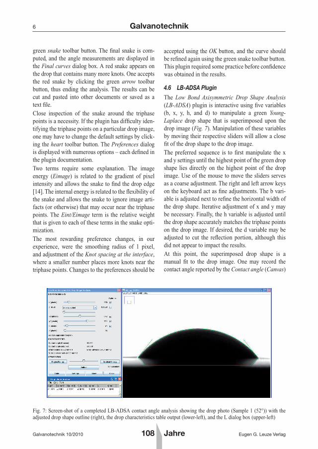
4.6 LB-ADSAPlugin

The Low Bond Axisymmetric Drop Shape Analysis (LB-ADSA) plugin is interactive using five variables (b, x, y, h, and d) to manipulate a green Young-Laplace drop shape that is superimposed upon the drop image (Fig. 7). Manipulation of these variables by moving their respective sliders will allow a close fit of the drop shape to the drop image.The preferred sequence is to first manipulate the x and y settings until the highest point of the green drop shape lies directly on the highest point of the drop image. Use of the mouse to move the sliders serves as a coarse adjustment. The right and left arrow keys on the keyboard act as fine adjustments. The b vari-able is adjusted next to refine the horizontal width of the drop shape. Iterative adjustment of x and y may be necessary. Finally, the h variable is adjusted until the drop shape accurately matches the triphase points on the drop image. If desired, the d variable may be adjusted to cut the reflection portion, although this did not appear to impact the results.At this point, the superimposed drop shape is a manual fit to the drop image. One may record the contact angle reported by the Contact angle (Canvas)

Fig. 7: Screen-shot of a completed LB-ADSA contact angle analysis showing the drop photo (Sample 1 (52°)) with the adjusted drop shape outline (right), the drop characteristics table output (lower-left), and the L dialog box (upper-left)

7


Galvanotechnik


line in the dialog box. With the outline correctly ori-ented around the drop image, an optimization of the drop shape may be initiated by clicking the Gradi-ent Energy button. The b, x, y, and h variables have checkboxes labeled Optimize next to them. Check marks indicate that these variables are active for opti-mization using the contrast between the drop and the background.

In like manner to DropSnake, this plugin uses the gradient-based edge detection that locates the point of greatest contrast along the drop edge. Thus, the optimization procedure is more likely to find the exact drop edge if the drop image under analysis pos-sesses a stark black and white contrast.

Post-optimization inspection of the drop shape is nec-essary, because the optimization may shift the drop shape substantially. If the refinement is acceptable, a click of the Table button will display the results in a window labeled Drop characteristics.

The LB-ADSA plugin should not be used when ana-lyzing drops lacking symmetry or images that are not level. Image tilt can introduce significant error, and this plugin will not provide individual values for the left and right contact angles of an asymmetric drop.

While the purpose of this work concerns LB-ADSA’s ability to measure contact angle, it is worth noting that the plugin also reports other geometric values of the drop such as drop volume, drop-air surface area, and drop-solid interface area. To display these, the user must input the proper pixel/millimeter conver-sion factor under the Settings button to the right of Table (Fig. 7). Additionally, input of the liquid’s cap-illary constant, which appears as the variable c in the LB-ADSA dialog box, allows for accurate correction for gravitational deformation of the drop. This was set to zero for our spherical ball lenses.

5 ResultsandDiscussion

The spherical samples used in this work allowed a very accurate measurement of the contact angle using the half-angle method. In ImageJ, a rectangular box was drawn that connected the apex of the circle to the two triphase points. The dimensions of this rectangle were recorded in pixels. The procedure was repeated three times to compute the uncertainty in the contact angle measurement. The range of uncertainty in the selection of height and width was less than 5 pixels. These height (h) and width (b) values were used with

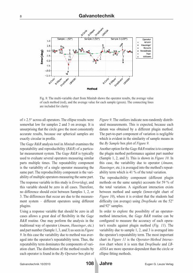
Equation <1> to produce the accepted contact angle values in Table 2.Six of the listed authors participated in the study. Each participant (labeled operator in the statistical analysis) used all three plugins to measure the contact angle of all three samples. These three samples are labeled Sample 1 (52°), Sample 2 (92°) and Sample 3 (120°) in the statistical analysis. The Brugnara plugin uses two methods (circle and ellipse) which, together with DropSnake and LB-ADSA, yields four methods of contact angle determination. These (B-Circle, B-Ellipse, DropSnake, and LB-ADSA) are labeled method in the statistical analysis.The statistical software package Minitab [16] was used to evaluate the data. One useful tool avail-able in Minitab is the multi-variable chart (Fig. 8). The response variable is absolute error (labeled Error(deg)) which is computed as measured CA minus accepted CA. Of course, the desired response is zero. Negative responses indicate that the mea-surement is less than the accepted value and vice versa. The abscissa is divided into three panels by sample. The center of each panel contains a green datum which is the average of all measurements for that sample. Each sample panel is divided into the four methods with red data indicating the average of that method for that sample. The individual opera-tor results are clustered within each method region. One can see the scatter (or otherwise) of the operator using each method on any given sample.It is evident from Figure 8 that DropSnake is very operator-dependent. The tightest distribution was the use of LB-ADSA on Sample 3 (120°), but LB-ADSA showed the most operator variation on Sample 2 (90°). In general, Brugnara’s plugin was least depen-dent upon operator with errors well within the range

Tab.2:Theacceptedvalues(Half-AngleCA)forthethreestandardsamples

Sample Half-Angle CA

Standard Deviation

Obtuse (ruby ball in 13/64” hole)

119.58° 0.14°

Near-normal (sapphire half-ball lens)

91.75° 0.46°

Acute (ruby ball protrusion through a 15/64” hole)

51.91° 0.72°

8


Galvanotechnik


Fig. 8: The multi-variable chart from Minitab shows the operator results, the average value of each method (red), and the average value for each sample (green). The connecting lines are included for clarity

of ± 2.5° across all operators. The ellipse results were somewhat low for samples 2 and 3 on average. It is unsurprising that the circle gave the most consistently accurate results, because our spherical samples are exactly circular in profile.

The Gage R&R analysis tool in Minitab examines the repeatability and reproducibility (R&R) of a particu-lar measurement system. The Gage R&R is typically used to evaluate several operators measuring similar parts multiple times. The repeatability component is the variability of a single operator measuring the same part. The reproducibility component is the vari-ability of multiple operators measuring the same part.

The response variable in this study is Error(deg), and this variable should be zero in all cases. Therefore, no difference should exist between Samples 1, 2, or 3. The differences that occur are due to the measure-ment system – different operators using different plugins.

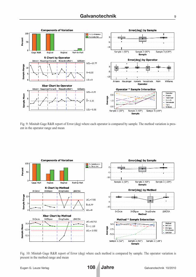
Using a response variable that should be zero in all cases allows a great deal of flexibility in the Gage R&R routine. One may perform the analysis in the traditional way of operator (Amann, Hausinger, etc.) and part number (Sample 1, 3, and 3) as seen in Figure 9. In this case the variability due to method was aver-aged into the operator’s repeatability term. Thus, the repeatability term dominates the components of vari-ation chart. The distribution of the method results by each operator is found in the By Operator box plot of

Figure 9. The outliers indicate non-randomly distrib-uted measurements. This is expected, because each datum was obtained by a different plugin method. The part-to-part component of variation is negligible which is evident in the similarity of sample means in the By Sample box plot of Figure 9.

Another option for the Gage R&R routine is to compare the plugin method performance against part number (Sample 1, 2, and 3). This is shown in Figure 10. In this case, the variability due to operator (Amann, Hausinger, etc.) is averaged into the method’s repeat-ability term which is 41 % of the total variation.

The reproducibility component (different plugin methods on the same sample) accounts for 59 % of the total variation. A significant interaction exists between method and sample (lower-right chart of Figure 10), where it is evident that the students had difficulty (on average) using DropSnake on the 52° and 92° samples.

In order to explore the possibility of an operator-method interaction, the Gage R&R routine can be configured to measure the accuracy of each opera-tor’s results against plugin method (Fig. 11). The variability due to sample 1, 2, and 3 is averaged into the operator’s repeatability term. The most important chart in Figure 11 is the Operator-Method Interac-tion chart where it is seen that DropSnake and LB-ADSA are more operator-dependent than the circle or ellipse fitting methods.

9


Galvanotechnik


Fig. 9: Minitab Gage R&R report of Error (deg) where each operator is compared by sample. The method variation is pres-ent in the operator range and mean

Fig. 10: Minitab Gage R&R report of Error (deg) where each method is compared by sample. The operator variation is present in the method range and mean

10


Galvanotechnik


6 Conclusions

The primary purpose of this work was to demonstrate that contact angles of sessile drops can be accurately measured using very low-cost equipment in conjunc-tion with open-access computer programs. Three such programs, each based on a different drop model were used and their results compared, using statisti-cal analysis. The results obtained were discussed in terms of the quality of the droplet image required in each case, susceptibility to operator error and limita-tions such as angle of tilt or drop symmetry, which some programs handle, while others do not.

Each of the three models has strengths and weak-nesses. The Brugnara plugin was the easiest to learn and the least susceptible to image tilt. DropSnake was difficult to use at first, but became quite easy once high-contrast image illumination was achieved via the apparatus presented in Figure 3. DropSnake was able to accommodate image tilt, and is the only option for highly asymmetric drops such as those used in advancing-receding contact angle studies.

Precision was addressed throughout the Gage R&R figures, and the multi-variable chart of Figure 8. The least precise method was the DropSnake plugin (cf. Error(deg) by Method in Fig. 10). The LB-ADSA

Fig. 11: Minitab Gage R&R report of Error(deg) where each operator is compared by method. The sample variation is present in the operator range and mean

plugin exhibited sample-dependent precision (cf. R Chart in Fig. 10). Brugnara’s plugin exhibited the least amount of sample-dependent variability in pre-cision (cf. R Chart in Fig. 10).

The evaluation of accuracy required stable standard samples – a spherical ball in a hole and a half-ball lens on a surface. The accepted value (i.e. Error(deg) = 0°) was contained within the range of values for each plugin with the exception of the DropSnake method on Sample 2 (92°) (Fig. 9). The plugins in aggregate erred towards underestimation of the contact angle, with an overall mean of Error(deg) equal to -1.1°.

Finally, successful training (or otherwise) was very easy to assess using these standard samples and the Gage R&R analysis. Once a participant had been trained in each of the plugins, their work could be evaluated for its reliability and whether the expected range of variability was achieved. Any problems were evident on the R chart. If an operator did not under-stand how to use the plugins properly, the R Chart showed repeatability problems for that operator. If the operator consistently obtained the wrong answer, the XBar Chart indicated that the mean of their mea-surements stood apart from the group. This analysis quickly identified who needed refresher training on the measurement techniques.

11


Galvanotechnik


AcknowledgementsThe previous research students of the Williams Group at Sam Houston State University (Trisha O’Bryon, Nelson Sheppard, Blake Howard, and Bryan Crom) are acknowledged for their hard work, curiosity, and cre-ative ideas related to this project. Dustin Palm is also acknowledged for his participation in the statistical study.

References[1] T. Phil. Young; Trans R Soc Lond 1805, 95, 65–87[2] ASTM Standard D 7334, 2008: Standard Practice for Surface Wet-

tability of Coatings, Substrates and Pigments by Advancing Contact Angle Measurement; ASTM International, West Conshohocken, PA, 2008, DOI: 10.1520/D7334-08, http://www.astm.org. (and included references)

[3] A. W. Adamson, A. P. Gast: Physical Chemistry of Surfaces; 6th Ed., Wiley-Interscience, New York, NY, 1997

[4] C. M. Hansen: Hansen Solubility Parameters – A User’s Handbook; 2nd Ed. CRC Press LLC, Boca Raton, FL, Chapter 6, 2007

[5] M. E. Schrader, G. I. Loeb: Modern Approaches to Wettability – Theory and Applications; Plenum Press, New York, NY, 1992

[6] R. Wright, M. Blitshteyn: Method and Apparatus for Measuring Contact Angles of Liquid Droplets on Substrate Surfaces; U.S. Patent 5,268,733, Dec. 7, 1993

[7] P. G. Wapner, W. P. Hoffman: Liquid to Solid Angle of Contact Measurement; U.S. Patent 6,867,854, Mar. 15, 2005; and referenced patents therein

[8] CorelDraw, version X5, Corel Corp., Mountain View, CA 2010

[9] Adobe Photoshop, version CS5, Adobe Systems Inc., San Jose, CA 2010

[10] W. S. Rasband: ImageJ, U. S. National Institutes of Health, Bethesda, Maryland, USA, http://rsb.info.nih.gov/ij/ (accessed July 2010), 1997–2010

[11] A. R. Stalder, T. Melchior, M. Muller, D. Sage, T. Blu, M. Unser: Low-Bond Axisymmetric Drop Shape Analysis for Surface Tension and Contact Angle Measurements of Sessile Drops; Colloids Surf A, 2010, 364, 72–81

[12] F. Thomsen: Practical Contact Angle Measurement – Measuring With Method – But With Which One?; KRÜSS Newsletter, 2008, 19, [Online] KRÜSS GmbH, Hamburg, Germany http://www.kruss.de/en/newsletter/newsletter-archives/2008/issue-19/application/ application-02.html (accessed July 2010)

[13] M. Brugnara: Contact Angle Plugin; University of Trento, Trento, Italy 2010

[14] A. F. Stalder, G. Kulik, D. Sage, L. Barbieri, P. Hoffmann: A Snake-based Approach to Accurate Determination of Both Contact Points and Contact Angles; Colloids Surf A, 2006, 286, 92–103

[15] R. Deriche: Using Canny’s Criteria to Derive a Recursively Imple-mented Optimal Edge Detector; Int. J. Computer Vision, 1987, 1, 167–187

[16] Minitab, version 14, Minitab Inc., State College, PA 2010

computerised measurement of contact angles

Documents