Ms

KD

a

ARRAA

KHSC

1

wstcp

cpcv(caacst

h0

Computers and Chemical Engineering 93 (2016) 413–427

Contents lists available at ScienceDirect

Computers and Chemical Engineering

j ourna l ho me pa g e: www.elsev ier .com/ locate /compchemeng

odel based approach to synthesize spare-supported cleaningchedules for existing heat exchanger networks

ai-Yuan Cheng, Chuei-Tin Chang ∗

epartment of Chemical Engineering, National Cheng Kung University, Tainan, 70101, Taiwan

r t i c l e i n f o

rticle history:eceived 19 December 2015eceived in revised form 27 June 2016ccepted 28 June 2016vailable online 29 June 2016

eywords:eat-exchanger networkpareleaning schedule

a b s t r a c t

Almost every modern chemical process is equipped with a heat-exchanger network (HEN) for optimalenergy recovery. However, as time goes on after startup, fouling on the heat-transfer surface in an indus-trial environment is unavoidable. If the heat exchangers in an operating plant are not cleaned regularly,the targeted thermal efficiency of HEN can only be sustained for a short period of time. To address thispractical issue, several mathematical programming models have already been developed to synthesizeonline cleaning schedules. Although the total utility cost of a HEN could be effectively reduced accordingly,any defouling operation still results in unnecessary energy loss due to the obvious need to temporarilytake the unit to be cleaned out of service. The objective of the present study is thus to modify the avail-able model so as to appropriately assign spares to replace them. Specifically, two binary variables areadopted to respectively represent distinct decisions concerning each online exchanger in a particulartime interval, i.e., whether it should be cleaned and, if so, whether it should be substituted with a spare.The optimal solution thus includes not only the cleaning schedule but also the total number of spares,their capacities and the substitution schedule. Finally, the optimization results of a series of case studiesare also presented to verify the feasibility of the proposed approach.

© 2016 Elsevier Ltd. All rights reserved.

. Introduction

In a chemical manufacturing process, efficient energy recovery and reuse is usually the key to minimizing the total operating cost,hile the heat exchanger network (HEN) is a viable vehicle for achieving such a purpose. After putting the units in a HEN in service, the

olid impurities in process streams may be deposited continuously on the heat-transfer surfaces and, thus, the overall performance of HENends to deteriorate over time. This fouling problem can be abated by cleaning all heat exchangers as a part of the overall maintenance (orheckup) program during plant shutdown. However, if it is also possible to clean at least a portion of the online units when the normalroduction is still in progress, then a proper schedule must be stipulated to maximize the implied cost saving.

A programming approach has often been adopted in the past to produce the aforementioned HEN cleaning schedules for energyonservation. To this end, Smaïli et al. (1999) first constructed a mixed integer nonlinear programming (MINLP) model for the thin-juicereheat train in a sugar refinery. Since the global solution of such a model cannot always be obtained, several additional studies have beenarried out to address the related computation issues. Georgiadis et al. (1999) tried to developed a mixed integer linear program (MILP)ia linearization of the nonlinear constraints so as to produce the near-optimum schedules efficiently, while Georgiadis and Papageorgiou2000) later studied solution strategies of the corresponding MINLP models. Alle et al. (2002) then solved a few example problems suc-essfully with the outer approximation algorithm. Smaïli et al. (2002) subsequently applied the simulated annealing, threshold acceptingnd backtracking threshold accepting algorithms to solve the models they first developed. Again for the same objective of achieving an

pproximate global optimum efficiently, Lavaja and Bagajewicz (2004) formulated a new MILP model via linearization to synthesize theleaning schedules. Their solutions were compared with those obtained in Smaïli et al. (2002) and it was found that both yielded similarchedules and roughly the same total annual costs. On the other hand, Markowski and Urbaniec (2005) suggested using a graphic methodo analyze the effects of fouling on the exit temperatures of every unit in a HEN and to manipulate the cleaning schedules accordingly.

∗ Corresponding author.E-mail addresses: ctchang@mail.ncku.edu.tw, chueitinchang@msn.com (C.-T. Chang).

ttp://dx.doi.org/10.1016/j.compchemeng.2016.06.020098-1354/© 2016 Elsevier Ltd. All rights reserved.

414 K.-Y. Cheng, C.-T. Chang / Computers and Chemical Engineering 93 (2016) 413–427

Nomenclature

SetsE The set of all exchanger labels in the given HENI The set of all hot-stream labels in the given HENJ The set of all cold-stream labels in the given HENPk The set of all period labels in year k of the time horizon

VariablesAsp Heat-transfer area of a spare exchanger (m2)

afm,tpi,j,k,p

The overall heat-transfer coefficient determined according to fouling model fm ∈{

L, E}

at time point tp ∈{bcp, ecp, bop, eop

}during period p (p ≥ 2) in scenario (i) if exchanger (i, j) ∈ E is last cleaned during period k and 1 ≤ k < p

(kW/m2 K)cfm,tp

i,j,pThe overall heat-transfer coefficient determined according to fouling model fm ∈

{L, E

}at time point tp ∈{

bcp, ecp, bop, eop}

during period p in scenario (iii) (kW/m2 K)

EuHj,p

, EuCi,p

Estimates of the total hot and cold utility consumption levels needed respectively by cold stream j ∈ J and hot stream i ∈I in period p (kW-mon)

Nsp Total number of sparesQuH,tp

j,p, QuC,tp

i,pThe hot and cold utility consumption rates needed respectively by cold stream j ∈ J and hot stream i ∈ I at time point

tp ∈{

bcp, ecp, bop, eop}

in period p (kW)ri,j The fouling resistance of heat exchanger (i, j) ∈ E (m2 K/kW)

TH,tpin,i,p

, TH,tpout,i,p

The inlet and outlet temperatures of hot stream i ∈ I of exchanger (i, j) ∈ E at time point tp ∈{

bcp, ecp, bop, eop}

inperiod p (K)

TC,tpin,j,p

, TC,tpout,j,p

The inlet and outlet temperatures of cold stream j ∈ J of exchanger(i, j) ∈ E at time point tp ∈{

bcp, ecp, bop, eop}

inperiod p (K)

TLH,tpi,p

, TLC,tpj,p

The outlet temperatures of hot and cold streams respectively from the last heat exchangers on streams i ∈ I and j ∈ J

at time point tp ∈{

bcp, ecp, bop, eop}

in period p (K)

Ufm,tpi,j,p

The overall heat-transfer coefficients of exchanger(i, j) at time point tp ∈{

bcp, ecp, bop, eop}

in period p determined

according to fouling model fm ∈{

L, E}

(kW/m2 K)X

i,j,pA binary variable used to denote whether or not a spare is adopted to replace exchanger (i, j) ∈ E during period p

Yi,j,p A binary variable used to denote whether or not exchangerer (i, j) ∈ E is cleaned during period p

ParametersAi,j The heat-transfer area of exchanger (i, j) ∈ E (m2)

bspfm,tpi,j,p

The overall heat-transfer coefficient determined according to fouling model fm ∈{

L, E}

at time point tp ∈{bcp, ecp, bop, eop

}during period p in scenario (ii) if a spare is adopted to replace exchanger (i, j) ∈ E (kW/m2 K)

CHi

, CCj

The heat capacities of hot stream i ∈ I and cold stream j ∈ J (kJ/kg-K)

CHUp , CCU

p The unit costs of heating and cooling utilities in period p ($/kJ)Ccl, Csp

clThe cleaning costs of a heat exchanger and a spare ($/cleaning)

Csp Annualized cost coefficient for the capital cost of heat exchanger(

$/m1.6yr)

fc The duration of a defouling sub-period (mon)FH

i, FC

jThe mass flow rates of hot stream i ∈ I and cold stream j ∈ J (kg/s)

Ki,j The characteristic fouling speed of exchanger (i, j) ∈ E (mon−1)Ri,j The ratio between the products of mass flow rate and heat capacity of the cold and hot streams in heat exchanger (i, j) ∈ Eri,j The constant fouling rate of exchanger (i, j) ∈ E (m2 K/mon kW)r∞

i,jThe asymptotic maximum fouling resistance of exchanger (i, j) ∈ E (m2 K/kW)

tf The overall time horizon (mon)TTH

i, TTC

jThe target temperatures of hot stream i ∈ I and cold stream j ∈ J (K)

Ucli,j

, Uclsp The overall heat-transfer coefficients of exchanger (i, j) ∈ E and spare exchanger when the heat-transfer surface is clean

(kW/m2 K)�p The length of period p (mon)�cl Efficiency of cleaning operation�H, �C The heat-transfer efficiencies in heater and cooler respectively

K.-Y. Cheng, C.-T. Chang / Computers and Chemical Engineering 93 (2016) 413–427 415

Superscriptsbcp The time point at the beginning of cleaning sub-periodbop The time point at the beginning of operation sub-periodecp The time point at the end of cleaning sub-periodeop The time point at the end of operation sub-periodE The exponential fouling modelL The linear fouling model

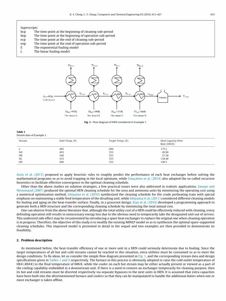
Fig. 1. Flow diagram of HEN considered in Example 1.

Table 1Stream data of Example 1.

Stream Inlet Temp. (K) Target Temp. (K) Heat Capacity FlowRate (kW/K)

C 405 606 175.2HA 493 353 49.98HB 540 353 27.28

Amh

Naefg

dTicf

2

tdsHtihm

HC 553 353 138.48HD 606 353 140.3

ssis et al. (2013) proposed to apply heuristic rules to roughly predict the performance of each heat exchanger before solving theathematical programs so as to avoid trapping in the local optimum, while Gonc alves et al. (2014) also adopted the so-called recursive

euristics to facilitate effective convergence to the optimal cleaning schedule.Other than the above studies on solution strategies, a few practical issues were also addressed in realistic applications. Sanaye and

iroomand (2007) produced the optimal HEN cleaning schedule for the urea and ammonia units by minimizing the operating cost using numerical optimization method. Ishiyama et al. (2010) synthesized the cleaning schedule for the crude preheating train with specialmphasis on maintaining a stable feed temperature of the desalting unit, while Ishiyama et al. (2011) considered different cleaning modelsor fouling and aging on the heat-transfer surface. Finally, in a grassroot design, Xiao et al. (2010) developed a programming approach toenerate both a HEN structure and the corresponding cleaning schedule by minimizing the total annual cost.

One can observe from the above literature that, although the total utility cost of a HEN could be effectively reduced with cleaning, everyefouling operation still results in unnecessary energy loss due to the obvious need to temporarily take the designated unit out of service.his undesired side effect may be circumvented by introducing a spare heat exchanger to replace the original one when cleaning operations in progress. Therefore, the objective of this study is to modify the existing MINLP model so as to synthesize the optimal spare-supportedleaning schedules. This improved model is presented in detail in the sequel and two examples are then provided to demonstrate itseasibility.

. Problem description

As mentioned before, the heat-transfer efficiency of one or more unit in a HEN could seriously deteriorate due to fouling. Since thearget temperatures of all hot and cold streams cannot be reached in this situation, extra utilities must be consumed so as to meet theesign conditions. To fix ideas, let us consider the simple flow diagram presented in Fig. 1, and the corresponding stream data and designpecifications given in Tables 1 and 2 respectively. The furnace in this process is obviously adopted to raise the cold outlet temperature ofE4 (494 K) to the final temperature of 606 K, while the cooler on each hot stream may be either actually present or viewed as a part of

he cooling capability embedded in a downstream unit. If there is a need to remove an exchanger temporarily for cleaning purpose, then

ts hot and cold streams must be diverted respectively via separate bypasses to the next units in HEN. It is assumed that extra capacitiesave been built into the aforementioned furnace and coolers so that they can be manipulated to handle the additional duties when one orore exchanger is taken offline.

416 K.-Y. Cheng, C.-T. Chang / Computers and Chemical Engineering 93 (2016) 413–427

Table 2Design specifications of heat exchangers in Example 1.

Heat Exchanger Ucli,j

(kW/m2 K) Ai,j(m2) Cold Stream Inlet and Outlet Temp. (K) Hot Stream Inlet and Outlet Temp. (K) Heat Duty (kW)

HE1 0.5 43.2 405/413 493/463 1401.6HE2 0.5 26.7 413/421 540/492 1401.6HE3 0.5 110.7 421/452 553/514 5431.2HE4 0.5 138.2 452/494 606/553 7358.4

crsp

123

Tet(pt

3

baio

wrpcc

wy

Fig. 2. Time horizon partitioning.

Since the fouling-related costs are affected by a large number of contributing factors, e.g., the given HEN structure, the duration of eachleaning operation, the corresponding heat load that must be taken out of service, the capacity of spare used to replace this service and theequired capital investment, etc., a programming approach is needed to synthesize the optimal defouling and spare substitution schedulesimultaneously so as to minimize the total annual cost (TAC). For model simplicity, the following assumptions have been adopted in theresent work:

. All cleaning durations are fixed at a predetermined constant value;

. All cleaning operations cost the same and this value is given a priori;

. Only identical spares are allowed.

The inputs to the proposed mathematical programming model should include: the original HEN design data (such as those given inable 1, Table 2 and Fig. 1), the heat-transfer models (i.e., the fouling resistance function, the cleaning efficiency and the heat-recoveryfficiencies of utility heaters and coolers), the time-horizon partition scheme (i.e., the total length of time horizon, the time interval betweenwo consecutive cleaning operations and a constant time duration allocated for every defouling operation), and also various cost modelsi.e., the unit costs of hot and cold utilities, the operating cost for cleaning an exchanger, and the capital cost model for a spare). Solving theroposed model should produce the following results: (1) the optimal cleaning and spare substitution schedules, (2) the number of spareso be purchased and their heat-transfer areas, and (3) the total utility cost, the total cleaning cost and the total capital investment.

. Time horizon partitioning

In this work, the maximum length of time horizon that can be considered for schedule synthesis (say tf ) is the duration in monthsetween the ending and beginning instances of two consecutive planned plant shutdowns. To simplify calculation, the entire duration of

cleaning schedule for a given HEN is set to be coincided with this time interval. In addition, the schedule horizon [0, tf ] is partitionednto n different periods according to Fig. 2 and each is further divided into two intervals for performing the cleaning and heat-exchangeperations respectively. For simplification purpose, the aforementioned time periods are fixed, i.e.

�1 = �2 = · · · = �n = � (1)

tf =n∑

p=1

�p = n� (2)

here, �p denotes the length of period p (p = 1, 2, · · ·, n) and � is a given constant. Also, it is assumed that the durations of all sub-periodsequired for defouling (fc) are the same and their values can be determined in advance. Thus, within each partitioned period, four timeoints should be identified to facilitate accurate presentation of the proposed model, i.e., bcp (beginning of cleaning sub-period), ecp (end ofleaning sub-period), bop (beginning of operation sub-period), and eop (end of operation sub-period). Finally, for the sake of computationonvenience, let us further assume that

tf = 12 × Itf (3)

here Itf is a nonnegative integer. To facilitate clear explanation of the multi-year cleaning schedule, let us define a period set for each

ear, i.e.

Pk ={

p | p is the numerical label of a period in year k of the cleaning schedule}

(4)

4

w

5

b

wc

w

6

t

wte

wa

7

oc(vt

7

K.-Y. Cheng, C.-T. Chang / Computers and Chemical Engineering 93 (2016) 413–427 417

. Binary variables to facilitate exchanger-cleaning selections

For illustration convenience, let us introduce the following two label sets to collect and classify the process streams in a given HEN:

I ={

i | i is the label of a hot stream in a given HEN}

(5)

J ={

j | j is the label of a cold stream in a given HEN}

(6)

In addition, the heat exchangers in this HEN can be written as

E ={

(i, j) | (i, j) denotes an exchanger in a given HEN, i ∈ I, j ∈ J}

(7)

Therefore, the selections of exchangers to be cleaned can be expressed accordingly with the following binary variable:

Yi,j,p ={

1 if heat exchanger (i, j) is cleaned in period p

0 otherwise(8)

here, (i, j) ∈ E and p = 1, 2, · · ·, n. Finally, for formulation simplicity, let us set Yi,j,0 = 0 in the proposed model.

. Binary variables to represent spare-substitution options

The need to consider a spare only arises after making the decision to remove and clean an online unit from HEN. All such options cane represented with another set of binary variables and the corresponding logic constraints, i.e.

Xi,j,p ={

1 if heat exchanger (i, j) is replaced with a spare in period p

0 otherwise(9)

(1 − Yi,j,p

)+ Xi,j,p ≤ 1 (10)

here, (i, j) ∈ E and p = 1, 2, · · ·, n. To set the upper limit for capital investment, it may also be necessary to impose the following inequalityonstraints:∑

(i,j) ∈ E

Xi,j,p ≤ Nsp ≤∑

(i,j) ∈ E

Yi,j,p (11)

here, Nsp is the maximum number of purchased spares and it is a given model parameter.

. Fouling models

As a result of fouling during the normal operation, the overall heat-transfer coefficient of every exchanger in HEN may decrease withime according to the following formula (Lavaja and Bagajewicz, 2004)

Ui,j (t) =[

1

Ucli,j

+ ri,j (t)

]−1

(12)

here, (i, j) ∈ E; Ui,j (t) is the overall heat-transfer coefficient of exchanger (i, j) at time t and Ucli,j

denotes the corresponding value whenhe heat-transfer surface is clean. The time function ri,j (t) is the fouling resistance of exchanger (i, j) at time t, which can be expressed withither a linear or exponential model:

ri,j (t) = ri,jt (13)

ri,j(t) = r∞i,j

[1 − exp(−Ki,jt)] (14)

here, ri,j denotes the constant fouling rate, r∞i,j

is the asymptotic maximum fouling resistance, Ki,j is the characteristic fouling speed, andll of them are given model parameters.

. Model constraints

Only the model constraints established on the basis of the linear fouling assumption are presented in the present section for the sakef brevity, while the corresponding formulations derived from the exponential model can be found in Appendix A. Basically both sets ofonstraints can be established by introducing the spare-substitution options into the existing model framework developed by Smaïli et al.1999, 2002) and Lavaja and Bagajewicz (2004). Note that the superscripts L and tp in the subsequent discussions are used to denote aariable (or parameter) associated with the linear model and time point tp ∈

{bcp, ecp, bop, eop

}respectively. An accurate description of

he corresponding model can be presented accordingly in the sequel:

.1. Overall heat transfer coefficients

Exactly three scenarios should be considered in modeling the overall heat-transfer coefficient in period p:

4

(

e

w

i

pM

N

d

Tdt

b

w

i

di

N

18 K.-Y. Cheng, C.-T. Chang / Computers and Chemical Engineering 93 (2016) 413–427

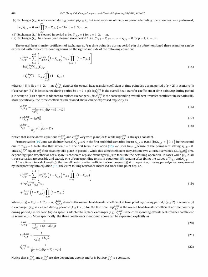
(i) Exchanger (i, j) is not cleaned during period p (p ≥ 2), but in at least one of the prior periods defouling operation has been performed,

i.e., Yi,j,p = 0 and

p−1∏k=1

(1 − Yi,j,k) = 0 for p = 2, 3, · · ·, n.

(ii) Exchanger (i, j) is cleaned in period p, i.e., Yi,j,p = 1 for p = 1, 2, · · ·, n.iii) Exchanger (i, j) has never been cleaned since period 1, i.e., Yi,j,1 = Yi,j,2 = · · · = Yi,j,p = 0 for p = 1, 2, · · ·, n.

The overall heat-transfer coefficient of exchanger (i, j) at time point bcp during period p in the aforementioned three scenarios can bexpressed with three corresponding terms on the right-hand side of the following equation:

UL,bcpi,j,p

=p−1∑k=0

[aL,bcp

i,j,k,p

(1 − X

i,j,p

)Yi,j,k

p∏v=k+1

(1 − Yi,j,v

)]

+bspL,bcpi,j,p

Xi,j,p

Yi,j,p

+ cL,bcpi,j,p

(1 − Xi,j,p

)

p∏z=0

(1 − Yi,j,z

)(15)

here, (i, j) ∈ E; p = 1, 2, · · ·, n; aL,bcpi,j,k,p

denotes the overall heat-transfer coefficient at time point bcp during period p (p ≥ 2) in scenario (i)

f exchanger (i, j) is last cleaned during period k (1 ≤ k < p); bspL,bcpi,j,p

is the overall heat-transfer coefficient at time point bcp during period

in scenario (ii) if a spare is adopted to replace exchanger (i, j); cL,bcpi,j,p

is the corresponding overall heat-transfer coefficient in scenario (iii).ore specifically, the three coefficients mentioned above can be expressed explicitly as

aL,bcpi,j,k,p

= 11

�clUcli,j

+ ri,j [(p − k) � − fc](16)

bspL,bcpi,j,p

= �clUclsp (17)

cL,bcpi,j,p

= 11

Ucli,j

+ ri,j (p − 1) �(18)

otice that in the above equations aL,bcpi,j,k,p

and cL,bcpi,j,p

vary with p and/or k, while bspL,bcpi,j,p

is always a constant.

From equation (10), one can deduce that (a) Xi,j,p = 0 in the first and third scenarios due to Yi,j,p = 0 and (b) Xi,j,p ∈{

0, 1}

in the second

ue to Yi,j,p = 1. Note also that, when p = 1, the first term in equation (15) vanishes b�clUclspecause of the permanent setting Yi,j,0 = 0.

hus, UL,bcpi,j,1 equals Ucl

i,jif no cleaning take place in period 1 while this same coefficient may assume two alternative values, i.e., �clU

clsp or 0,

epending upon whether or not a spare is chosen to replace exchanger (i, j) to facilitate the defouling operation. In cases when p ≥ 2, allhree scenarios are possible and exactly one of corresponding terms in equation (15) remains after fixing the values of Yi,j,p and Xi,j,p.

After a time interval of length fc , the overall heat-transfer coefficient of exchanger (i, j) at time point ecp during period p can be expressedy incorporating into equation (15) the extra fouling resistance increased since time point bcp, i.e.

UL,ecpi,j,p

=p−1∑k=0

[aL,ecp

i,j,k,p

(1 − X

i,j,p

)Yi,j,k

p∏v=k+1

(1 − Yi,j,v

)]

+bspL,ecpi,j,p

Xi,j,p

Yi,j,p

+cL,ecpi,j,p

(1 − X

i,j,p

) p∏z=0

(1 − Yi,j,z

)(19)

here, (i, j) ∈ E; p = 1, 2, · · ·, n; aL,ecpi,j,k,p

denotes the overall heat-transfer coefficient at time point ecp during period p (p ≥ 2) in scenario (i)

f exchanger (i, j) is cleaned during period k (1 ≤ k < p) for the last time; bspL,ecpi,j,p

is the overall heat-transfer coefficient at time point ecp

uring period p in scenario (ii) if a spare is adopted to replace exchanger (i, j); cL,ecpi,j,p

is the corresponding overall heat-transfer coefficientn scenario (iii). More specifically, the three coefficients mentioned above can be expressed explicitly as

aL,ecpi,j,k,p

= 11

�clUcli,j

+ (p − k) ri,j�(20)

bspL,ecpi,j,p

= 11

�clUclsp

+ ri,jfc(21)

cL,ecpi,j,p

= 11

Ucli,j

+ ri,j [(p − 1) � + fc](22)

otice that aL,ecpi,j,k,p

and cL,ecpi,j,p

are also dependent upon p and/or k, but bspL,ecpi,j,p

is a constant.

ff

w

b

A

o

w

id

N

7

wm

C

d(s

w

K.-Y. Cheng, C.-T. Chang / Computers and Chemical Engineering 93 (2016) 413–427 419

Note that, since exchanger (i, j) is not cleaned during period p in scenarios (i) and (iii), equations (20) and (22) should also be applicableor time point bop as well. Thus, the overall heat-transfer coefficient of exchanger (i, j) at instance bop during period p can be expressed asollows

UL,bopi,j,p

=p−1∑k=0

[aL,bop

i,j,k,pYi,j,k

p∏v=k+1

(1 − Yi,j,v

)]+ bL,bop

i,j,pYi,j,p + cL,bop

i,j,p

p∏z=0

(1 − Yi,j,z

)(23)

here, (i, j) ∈ E; p = 1, 2, · · ·, n; aL,bopi,j,k,p

(= aL,ecpi,j,k,p

) and cL,bopi,j,p

(= cL,ecpi,j,p

) have already been defined in equations (20) and (22) respectively;L,bopi,j,p

denotes the overall heat-transfer coefficient at time point bop during period p in scenario (ii), i.e.

bL,bopi,j,p

= �cUcli,j (24)

gain bL,bopi,j,p

here is a constant.Finally, the formulas for representing the overall heat-transfer coefficient of exchanger (i, j) at time point eop during period p can be

btained by introducing into equation (23) the additional fouling resistance increased since time point bop, i.e.

UL,eopi,j,p

=p−1∑k=0

[aL,eop

i,j,k,pYi,j,k

p∏v=k+1

(1 − Yi,j,v

)]+ bL,eop

i,j,pYi,j,p + cL,eop

i,j,p

p∏z=0

(1 − Yi,j,z

)(25)

here, (i, j) ∈ E; p = 1, 2, · · ·, n; aL,eopi,j,k,p

denotes the overall heat-transfer coefficient at time point eop during period p (p ≥ 2) in scenario (i)

f exchanger (i, j) is last cleaned during period k (1 ≤ k < p); bL,eopi,j,p

and cL,eopi,j,p

denote the overall heat-transfer coefficients at time point eopuring period p in scenarios (ii) and (iii) respectively. The aforementioned three coefficients can be written explicitly as

aL,eopi,j,k,p

= 11

�clUcli,j

+ ri,j [(p − k + 1) � − fc](26)

bL,eopi,j,p

= 11

�clUcli,j

+ ri,j (� − fc)(27)

cL,eopi,j,p

= 11

Ucli,j

+ ri,jp�(28)

ote that aL,eopi,j,k,p

and cL,eopi,j,p

are both variables depending upon p and/or k, and bL,eopi,j,p

is a constant.

.2. Exchanger inlet and outlet temperatures

By assuming pseudo counter-current flow in every heat exchanger, the corresponding energy balance can be written as

Qi,j (t) = FH

iCH

i

(TH

in,i (t) − THout,i (t)

)= FC

jCC

j

(TC

out,j (t) − TCin,j (t)

)

= Ui,j (t) Ai,j

(TH

in,i (t) − TCout,j (t)

)−

(TH

out,i (t) − TCin,j (t)

)ln

[(TH

in,i (t) − TCout,j (t)

)/(

THout,i (t) − TC

in,j (t))] (29)

here, (i, j) ∈ E; t ∈ [0, tf ]; Qi,j is the heat duty (kJ/s) of exchanger (i, j); Ai,j is the heat transfer area (m2) of exchanger (i, j) and it is a givenodel parameter; FH

iand FC

jdenote respectively the mass flow rates (kg/s) of hot stream i and cold stream j and they are model parameters;

Hi

and CCj

denote respectively the heat capacities (kJ/kg-K) of hot stream i and cold stream j and they are also model parameters; THin,i

and TCin,j

enote respectively the inlet temperatures (K) of hot stream i and cold stream j; THout,i

and TCout,j

denote respectively the outlet temperaturesK) of hot stream i and cold stream j. Equation (29) can then be rearranged to produce an expression for the outlet temperature of the hottream, i.e.

THout,i (t) =

(Ri,j − 1

)TH

in,i (t) +{

exp

[Ui,j(t)Ai,j

FCj

CCj

(Ri,j − 1

)]− 1

}Ri,jT

Cin,j (t)

Ri,j exp

[Ui,j(t)Ai,j

FCj

CCj

(Ri,j − 1

)]− 1

(30)

here, the constant R is defined as

i,j

Ri,j =FC

jCC

j

FHi

CHi

=TH

out,i (t) − THin,i (t)

TCin,j (t) − TC

out,j (t)(31)

4

wt

o

20 K.-Y. Cheng, C.-T. Chang / Computers and Chemical Engineering 93 (2016) 413–427

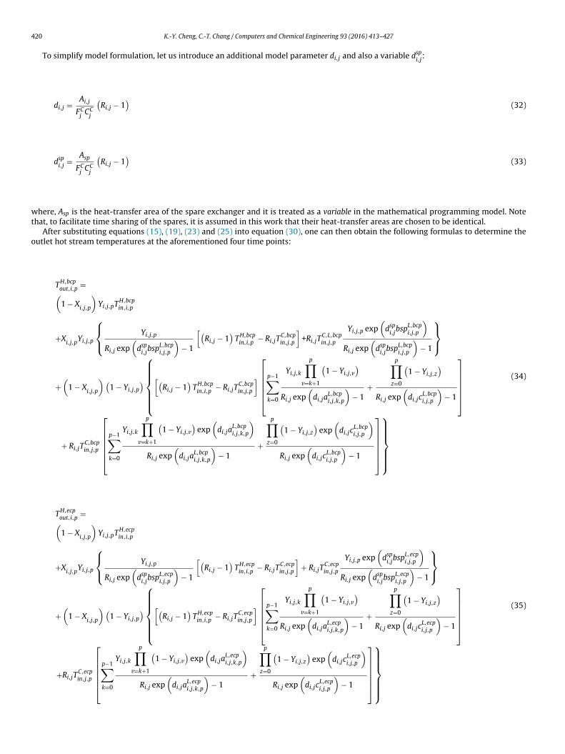
To simplify model formulation, let us introduce an additional model parameter di,j and also a variable dspi,j

:

di,j = Ai,j

FCj

CCj

(Ri,j − 1

)(32)

dspi,j

= Asp

FCj

CCj

(Ri,j − 1

)(33)

here, Asp is the heat-transfer area of the spare exchanger and it is treated as a variable in the mathematical programming model. Notehat, to facilitate time sharing of the spares, it is assumed in this work that their heat-transfer areas are chosen to be identical.

After substituting equations (15), (19), (23) and (25) into equation (30), one can then obtain the following formulas to determine theutlet hot stream temperatures at the aforementioned four time points:

TH,bcpout,i,p

=(1 − X

i,j,p

)Yi,j,pTH,bcp

in,i,p

+Xi,j,p

Yi,j,p

⎧⎨⎩ Yi,j,p

Ri,j exp(

dspi,j

bspL,bcpi,j,p

)− 1

[(Ri,j − 1

)TH,bcp

in,i,p− Ri,jT

C,bcpin,j,p

]+Ri,jT

C,L,bcpin,j,p

Yi,j,p exp(

dspi,j

bspL,bcpi,j,p

)Ri,j exp

(dsp

i,jbspL,bcp

i,j,p

)− 1

⎫⎬⎭

+(

1 − Xi,j,p

)(1 − Yi,j,p

)⎧⎪⎪⎪⎪⎨⎪⎪⎪⎪⎩

[(Ri,j − 1

)TH,bcp

in,i,p− Ri,jT

C,bcpin,j,p

]⎡⎢⎢⎢⎢⎣

p−1∑k=0

Yi,j,k

p∏v=k+1

(1 − Yi,j,v

)Ri,j exp

(di,ja

L,bcpi,j,k,p

)− 1

+

p∏z=0

(1 − Yi,j,z

)Ri,j exp

(di,jc

L,bcpi,j,p

)− 1

⎤⎥⎥⎥⎥⎦

+ Ri,jTC,bcpin,j,p

⎡⎢⎢⎢⎢⎣

p−1∑k=0

Yi,j,k

p∏v=k+1

(1 − Yi,j,v

)exp

(di,ja

L,bcpi,j,k,p

)

Ri,j exp(

di,jaL,bcpi,j,k,p

)− 1

+

p∏z=0

(1 − Yi,j,z

)exp

(di,jc

L,bcpi,j,p

)

Ri,j exp(

di,jcL,bcpi,j,p

)− 1

⎤⎥⎥⎥⎥⎦

⎫⎪⎪⎪⎪⎬⎪⎪⎪⎪⎭

(34)

TH,ecpout,i,p

=(1 − X

i,j,p

)Yi,j,pTH,ecp

in,i,p

+Xi,j,p

Yi,j,p

⎧⎨⎩ Yi,j,p

Ri,j exp(

dspi,j

bspL,ecpi,j,p

)− 1

[(Ri,j − 1

)TH,ecp

in,i,p− Ri,jT

C,ecpin,j,p

]+ Ri,jT

C,ecpin,j,p

Yi,j,p exp(

dspi,j

bspL,ecpi,j,p

)Ri,j exp

(dsp

i,jbspL,ecp

i,j,p

)− 1

⎫⎬⎭

+(

1 − Xi,j,p

)(1 − Yi,j,p

)⎧⎪⎪⎪⎪⎨⎪⎪⎪⎪⎩

[(Ri,j − 1

)TH,ecp

in,i,p− Ri,jT

C,ecpin,j,p

]⎡⎢⎢⎢⎢⎣

p−1∑k=0

Yi,j,k

p∏v=k+1

(1 − Yi,j,v

)Ri,j exp

(di,ja

L,ecpi,j,k,p

)− 1

+

p∏z=0

(1 − Yi,j,z

)Ri,j exp

(di,jc

L,ecpi,j,p

)− 1

⎤⎥⎥⎥⎥⎦

⎡⎢ p−1

Yi,j,k

p∏ (1 − Yi,j,v

)exp

(di,ja

L,ecpi,j,k,p

) p∏(1 − Yi,j,z

)exp

(di,jc

L,ecpi,j,p

)⎤⎥

⎫⎪⎪⎪⎪⎬

(35)

+Ri,jTC,ecpin,j,p

⎢⎢⎢⎣∑k=0

v=k+1

Ri,j exp(

di,jaL,ecpi,j,k,p

)− 1

+ z=0

Ri,j exp(

di,jcL,ecpi,j,p

)− 1

⎥⎥⎥⎦⎪⎪⎪⎪⎭

w

pp

wp

7

c

w

T

cpa

8

e

K.-Y. Cheng, C.-T. Chang / Computers and Chemical Engineering 93 (2016) 413–427 421

TH,bopout,i,p

=

[(Ri,j − 1

)TH,bop

in,i,p− Ri,jT

C,bopin,j,p

]⎡⎢⎢⎢⎢⎣

p−1∑k=0

Yi,j,k

p∏v=k+1

(1 − Yi,j,v

)Ri,j exp

(di,ja

L,bopi,j,k,p

)− 1

+ Yi,j,p

Ri,j exp(

di,jbL,bopi,j,p

)− 1

+

p∏z=0

(1 − Yi,j,z

)Ri,j exp

(di,jc

L,bopi,j,p

)− 1

⎤⎥⎥⎥⎥⎦

+Ri,jTC,bopin,j,p

⎡⎢⎢⎢⎢⎣

p−1∑k=0

Yi,j,k

p∏v=k+1

(1 − Yi,j,v

)exp

(di,ja

L,bopi,j,k,p

)

Ri,j exp(

di,jaL,bopi,j,k,p

)− 1

+Yi,j,p exp

(di,jb

L,bopi,j,p

)Ri,j exp

(di,jb

L,bopi,j,p

)− 1

+

p∏z=0

(1 − Yi,j,z

)exp

(di,jc

L,bopi,j,p

)

Ri,j exp(

di,jcL,bopi,j,p

)− 1

⎤⎥⎥⎥⎥⎦

(36)

TH,eopout,i,p

=

[(Ri,j − 1

)TH,eop

in,i,p− Ri,jT

C,eopin,j,p

]⎡⎢⎢⎢⎢⎣

p−1∑k=0

Yi,j,k

p∏v=k+1

(1 − Yi,j,v

)Ri,j exp

(di,ja

L,eopi,j,k,p

)− 1

+ Yi,j,p

Ri,j exp(

di,jbL,eopi,j,p

)− 1

+

p∏z=0

(1 − Yi,j,z

)Ri,j exp

(di,jc

L,eopi,j,p

)− 1

⎤⎥⎥⎥⎥⎦

+Ri,jTC,eopin,j,p

⎡⎢⎢⎢⎢⎣

p−1∑k=0

Yi,j,k

p∏v=k+1

(1 − Yi,j,v

)exp

(di,ja

L,eopi,j,k,p

)

Ri,j exp(

di,jaL,eopi,j,k,p

)− 1

+Yi,j,p exp

(di,jb

L,eopi,j,p

)Ri,j exp

(di,jb

L,eopi,j,p

)− 1

+

p∏z=0

(1 − Yi,j,z

)exp

(di,jc

L,eopi,j,p

)

Ri,j exp(

di,jcL,eopi,j,p

)− 1

⎫⎪⎪⎪⎪⎬⎪⎪⎪⎪⎭

⎤⎥⎥⎥⎥⎦

(37)

here, (i, j) ∈ E; p = 1, 2, · · ·, n; TH,tpout,i,p

denotes the outlet temperature of hot stream i at time point tp ∈{

bcp, ecp, bop, eop}

in period

; TH,tpin,i,p

and TC,tpin,j,p

denote respectively the inlet temperatures of hot stream i and clod stream j at time point tp ∈{

bcp, ecp, bop, eop}

ineriod p.

Finally, the outlet temperatures of cold stream at different time instances can be determined according to equation (31), i.e.

TC,tpout,j,p

= TC,tpin,j,p

+TH,tp

in,i,p− TH,tp

out,i,p

Ri,j(38)

here, (i, j) ∈ E; p = 1, 2, · · ·, n; tp ∈{

bcp, ecp, bop, eop}

; TC,tpout,j,p

denotes the outlet temperature of cold stream j at time point tp in period.

.3. Utility consumption rates

Since the original HEN design specifications are given, a straightforward computation can be performed to determine the utilityonsumption rate needed to bring the final temperature of each process stream to its target value.

QuH,tpj,p

= FCj CC

j

(TTC

j − TLC,tpj,p

)∀j ∈ J (39)

QuC,tpi,p

= FHi CH

i

(TLH,tp

i,p− TTH

i

)∀i ∈ I (40)

here, tp ∈{

bcp, ecp, bop, eop}

; TTCj

and TTHi

denote the target temperatures of cold stream j and hot steam i respectively; TLC,tpj,p

and

LH,tpi,p

denote the outlet temperatures of the last unit on cold stream j and hot steam i respectively at time point tp; QuH,tpj,p

is the hot utility

onsumption rate needed by cold stream j at time point tp; QuC,tpi,p

is the cold utility consumption rate needed by hot stream i at timeoint tp. Consequently, the total amounts of utilities consumed respectively by cold stream j and hot stream i in period p can be estimatedccording to the following formulas:

EuHj,p =

QuH,bcpj,p

+ QuH,ecpj,p

2fc +

QuH,bopj,p

+ QuH,eopj,p

2(� − fc) j ∈ J (41)

EuCi,p =

QuC,bcpi,p

+ QuC,ecpi,p

2fc +

QuC,bopi,p

+ QuC,eopi,p

2(� − fc) i ∈ I (42)

. Objective function – total annual cost

As mentioned before, the maximum length of time horizon allowed for schedule synthesis is chosen to be the duration between thending and beginning instances of two consecutive planned shutdowns, i.e. tf . The total annual cost (TAC) associated with operating and

422 K.-Y. Cheng, C.-T. Chang / Computers and Chemical Engineering 93 (2016) 413–427

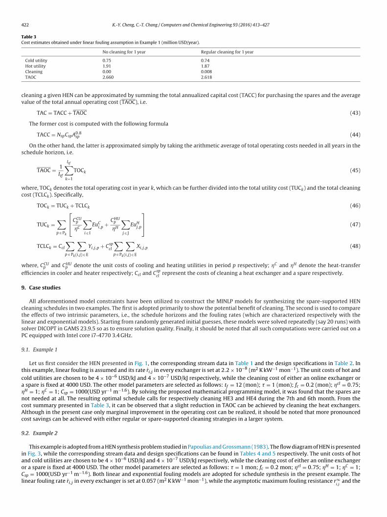
Table 3Cost estimates obtained under linear fouling assumption in Example 1 (million USD/year).

No cleaning for 1 year Regular cleaning for 1 year

Cold utility 0.75 0.74Hot utility 1.91 1.87

cv

s

wc

we

9

ctlsP

9

tca�ncAc

9

iaoCl

Cleaning 0.00 0.008TAOC 2.660 2.618

leaning a given HEN can be approximated by summing the total annualized capital cost (TACC) for purchasing the spares and the averagealue of the total annual operating cost (TAOC), i.e.

TAC = TACC + TAOC (43)

The former cost is computed with the following formula

TACC = NspCspA0.8sp (44)

On the other hand, the latter is approximated simply by taking the arithmetic average of total operating costs needed in all years in thechedule horizon, i.e.

TAOC = 1Itf

Itf∑k=1

TOCk (45)

here, TOCk denotes the total operating cost in year k, which can be further divided into the total utility cost (TUCk) and the total cleaningost (TCLCk). Specifically,

TOCk = TUCk + TCLCk (46)

TUCk =∑p ∈ Pk

⎡⎣CCU

p

�C

∑i ∈ I

EuCi,p + CHU

p

�H

∑j ∈ J

EuHj,p

⎤⎦ (47)

TCLCk = Ccl

∑p ∈ Pk

∑(i,j) ∈ E

Yi,j,p + Cspcl

∑p ∈ Pk

∑(i,j) ∈ E

Xi,j,p (48)

here, CCUp and CHU

p denote the unit costs of cooling and heating utilities in period p respectively; �C and �H denote the heat-transferfficiencies in cooler and heater respectively; Ccl and Csp

clrepresent the costs of cleaning a heat exchanger and a spare respectively.

. Case studies

All aforementioned model constraints have been utilized to construct the MINLP models for synthesizing the spare-supported HENleaning schedules in two examples. The first is adopted primarily to show the potential benefit of cleaning. The second is used to comparehe effects of two intrinsic parameters, i.e., the schedule horizons and the fouling rates (which are characterized respectively with theinear and exponential models). Starting from randomly generated initial guesses, these models were solved repeatedly (say 20 runs) witholver DICOPT in GAMS 23.9.5 so as to ensure solution quality. Finally, it should be noted that all such computations were carried out on aC equipped with Intel core i7-4770 3.4 GHz.

.1. Example 1

Let us first consider the HEN presented in Fig. 1, the corresponding stream data in Table 1 and the design specifications in Table 2. Inhis example, linear fouling is assumed and its rate ri,j in every exchanger is set at 2.2 × 10−8 (m2 K kW−1 mon−1). The unit costs of hot andold utilities are chosen to be 4 × 10−6 USD/kJ and 4 × 10−7 USD/kJ respectively, while the cleaning cost of either an online exchanger or

spare is fixed at 4000 USD. The other model parameters are selected as follows: tf = 12 (mon); � = 1 (mon); fc = 0.2 (mon); �cl = 0.75;H = 1; �C = 1; Csp = 1000(USD yr−1 m−1.6). By solving the proposed mathematical programming model, it was found that the spares areot needed at all. The resulting optimal schedule calls for respectively cleaning HE3 and HE4 during the 7th and 6th month. From theost summary presented in Table 3, it can be observed that a slight reduction in TAOC can be achieved by cleaning the heat exchangers.lthough in the present case only marginal improvement in the operating cost can be realized, it should be noted that more pronouncedost savings can be achieved with either regular or spare-supported cleaning strategies in a larger system.

.2. Example 2

This example is adopted from a HEN synthesis problem studied in Papoulias and Grossmann (1983). The flow diagram of HEN is presentedn Fig. 3, while the corresponding stream data and design specifications can be found in Tables 4 and 5 respectively. The unit costs of hot

nd cold utilities are chosen to be 4 × 10−6 USD/kJ and 4 × 10−7 USD/kJ respectively, while the cleaning cost of either an online exchangerr a spare is fixed at 4000 USD. The other model parameters are selected as follows: � = 1 mon; fc = 0.2 mon; �cl = 0.75; �H = 1; �C = 1;sp = 1000(USD yr−1 m−1.6). Both linear and exponential fouling models are adopted for schedule synthesis in the present example. The

inear fouling rate ri,j in every exchanger is set at 0.057 (m2 K kW−1 mon−1), while the asymptotic maximum fouling resistance r∞i,j

and the

K.-Y. Cheng, C.-T. Chang / Computers and Chemical Engineering 93 (2016) 413–427 423

Fig. 3. Flow diagram of HEN considered in Example 2.

Table 4Stream data of Example 2.

Stream Initial Temp. (K) Target Temp. (K) Heat Capacity FlowRate (kW/K)

H1 433 366 8.79H2 522 411 10.55H3 544 422 12.56H4 500 339 14.77H5 472 339 17.73C1 355 450 17.28C2 366 478 13.90C3 311 494 8.44C4 333 453 7.62C5 359 495 6.08

Table 5Design specifications of heat exchangers in Example 2.

Unit Ucli,j

(kW/m2 K) Ai,j(m2) Cold Stream Inlet and Outlet Temp. (K) Hot Stream Inlet and Outlet Temp. (K) Heat Duty (kW)

HE1 0.85 82.94 355/450 472/380 1641.6HE2 0.85 6.7 366/495 544/438 341.3HE3 0.85 38.2 366/474 500/418 1215.5HE4 0.85 4.33 311/353 445/411 173.1HE5 0.85 24.7 353/494 544/417 1191HE6 0.85 25.1 333/410 433/366 588.9HE7 0.85 3.26 410/433 522/453 644.5HE8 0.85 19.57 389/495 522/442 644.5CU1 0.85 32.68 311/355 418/339 1170.8CU2 0.85 33.16 311/355 380/339 718.2

424 K.-Y. Cheng, C.-T. Chang / Computers and Chemical Engineering 93 (2016) 413–427

Table 6Regular 1-year cleaning schedule in Example 2 (linear fouling).

Unit Month

1 2 3 4 5 6 7 8 9 10 11 12HE1 ©HE2 ©HE3 ©HE4 ©HE5 ©HE6 ©HE7 ©HE8 ©

©: regular cleaning operation.

Table 7Spare-supported 1-year cleaning schedule in Example 2 (linear fouling).

Unit Month

1 2 3 4 5 6 7 8 9 10 11 12HE1 �

HE2 � �

HE3 �

HE4 �

HE5 �

HE6 �

HE7 �

HE8 ©©: regular cleaning operation; �: spare-supported cleaning operation.

Table 8Spare-supported 2-year cleaning schedule in Example 2 (linear fouling).

Unit Month

6 7 8 9 10 11 12 13 14 15 16 17 18 19 20 21HE1 � � �

HE2 � � �

HE3 � � �

HE4 © © �

HE5 � � � �

HE6 � � �

HE7 © � �

HE8 � � �

©: regular cleaning operation; �: spare-supported cleaning operation.

Table 9Cost estimates obtained under linear fouling assumption in Example 2 (million USD/year).

No cleaning for 1 year No cleaning for 2 year Regular cleaning for 1 year Spare-supported cleaning for 1 year Spare-supported cleaning for 2 years

Cold U. 0.28 0.33 0.27 0.25 0.26Hot U. 0.52 0.95 0.39 0.27 0.24Cleaning 0.00 0.00 0.03 0.07 0.09

cHls

•

•

Spares 0.00 0.00 0.00 0.04 0.05TAC 0.80 1.28 0.69 0.63 0.64

haracteristic fouling speed Ki,j in the exponential model are chosen to be 0.684 (m2 K/kW) and 0.25 (mon−1) respectively for each unit inEN. Since in this case r∞

i,j= 12ri,j , the short-term fouling rate characterized by the exponential model should be larger than that by the

inear model. For illustration clarity, let us present and discuss the cleaning schedules generated on the basis of these two different modelseparately in sequence:

Tables 6 and 7 respectively shows the regular and spare-supported 1-year cleaning schedules obtained by solving the proposed mathe-matical programming models under the assumption of linear fouling. In the latter case, it was determined that two identical spares areneeded and each has a heat-transfer area of 35.95 m2. Table 8 shows the spare-supported cleaning schedule for an operation horizon of 2years. For this case, the computation time of each optimization run is approximately 9 s. Notice also that the number of spares needed toimplement this schedule is also 2 and they both have the same area of 51.61 m2. From the cost estimates of the 1-year cleaning schedulespresented in Table 9, it can be observed that roughly a saving of 18.8% TAC can be achieved with regular cleaning and a further reductionof 7.1% TAC if spares are adopted. However, by comparing the TACs of the 1-year and 2-year spare-supported cleaning schedules, one

can see that there are essentially no benefits to extend the horizon to a longer period.Tables 10 and 11 respectively shows the regular and spare-supported 1-year cleaning schedules obtained by solving the proposedmathematical programming models under the assumption of exponential fouling. The latter schedule only calls for one spare with aheat-transfer area of 69.14 m2. The optimal spare-supported 2-year cleaning schedule can be found in Table 12, and it took 40 s to

K.-Y. Cheng, C.-T. Chang / Computers and Chemical Engineering 93 (2016) 413–427 425

Table 10Regular 1-year cleaning schedule in Example 2 (exponential fouling).

Unit Month

1 2 3 4 5 6 7 8 9 10 11 12HE1 ©HE2 ©HE3 ©HE4 ©HE5 © ©HE6 ©HE7 © ©HE8 © ©

©: regular cleaning operation.

Table 11Spare-supported 1-year cleaning schedule in Example 2 (exponential fouling).

Unit Month

1 2 3 4 5 6 7 8 9 10 11 12HE1 �

HE2 ©HE3 � �

HE4 � �

HE5 © ©HE6 �

HE7 © ©HE8 © ©

©: regular cleaning operation; �: spare-supported cleaning operation.

Table 12Spare-supported 2-year cleaning schedule in Example 2 (exponential fouling).

Unit Month

4 5 6 7 8 9 10 11 12 13 14 15 16 17 18 19 20 21HE1 � � � �

HE2 � � � �

HE3 � � � �

HE4 � � �

HE5 � � � � � © �

HE6 � � �

HE7 © �

HE8 � � � � �

©: regular cleaning operation; �: spare-supported cleaning operation.

Table 13Cost estimates obtained under exponential fouling assumption in Example 2 (million USD/year).

No cleaning for 1 year No cleaning for 2 year Regular cleaning for 1 year Spare-supported cleaning for 1 year Spare-supported cleaning for 2 years

Cold U. 0.31 0.32 0.30 0.28 0.27Hot U. 0.76 0.875 0.67 0.51 0.39Cleaning 0.00 0.00 0.05 0.08 0.12

1

sbbbs

Spares 0.00 0.00 0.00 0.03 0.06TAC 1.07 1.195 1.02 0.90 0.84

complete each repeated optimization run. Notice also that the number of spares needed to implement this schedule is increased to 2and they both have the same area of 70.21 m2. From the cost estimates of the 1-year cleaning schedules presented in Table 13, it can beobserved that roughly a saving of 8.9% TAC can be achieved with regular cleaning and an additional reduction of another 8.9% TAC canalso be achieved with spares. Furthermore, by comparing the TACs of the spare-supported cleaning schedules, one can see that an extra6.7% decrease can be realized by extending the operation horizon from 1 to 2 years.

0. Conclusions

An improved mathematical programming model has been developed in this work to synthesize the optimal spare-supported cleaningchedule for any given heat exchanger network. The effectiveness of this approach has been verified with extensive case studies. It cane observed from the optimization results that spares are viable options for reducing the extra amount of utility consumption causedy temporarily removing online heat exchangers for cleaning purpose. In addition, potential financial benefit (in terms of TAC) may also

e realized by extending the schedule horizon to a longer period of time. These operation strategies are especially effective when thehort-term fouling rate is relatively large and thus cleaning is required more frequently.

4

A

M

fr

w

26 K.-Y. Cheng, C.-T. Chang / Computers and Chemical Engineering 93 (2016) 413–427

ppendix A.

odel constraints under exponential fouling assumption

The linear-fouling based formulations in section 7 can be easily converted to a second set of model constraints under the exponentialouling assumption, i.e. equation (14). Specifically, by replacing the superscript L with E, the overall heat transfer coefficients can beewritten as

UE,bcpi,j,p

=p−1∑k=0

[aE,bcp

i,j,k,p

(1 − X

i,j,p

)Yi,j,k

p∏v=k+1

(1 − Yi,j,v

)]

+bspE,bcpi,j,p

Xi,j,p

Yi,j,p

+cE,bcpi,j,p

(1 − X

i,j,p

) p∏z=0

(1 − Yi,j,z

)(A1)

UE,ecpi,j,p

=p−1∑k=0

[aE,ecp

i,j,k,p

(1 − X

i,j,p

)Yi,j,k

p∏v=k+1

(1 − Yi,j,v

)]

+bspE,ecpi,j,p

Xi,j,p

Yi,j,p

+cE,ecpi,j,p

(1 − X

i,j,p

) p∏z=0

(1 − Yi,j,z

)(A2)

UE,bopi,j,p

=p−1∑k=0

[aE,bop

i,j,k,pYi,j,k

p∏v=k+1

(1 − Yi,j,v

)]+ bE,bop

i,j,pYi,j,p + cE,bop

i,j,p

p∏z=0

(1 − Yi,j,z

)(A3)

UE,eopi,j,p

=p−1∑k=0

[aE,eop

i,j,k,pYi,j,k

p∏v=k+1

(1 − Yi,j,v

)]+ bE,eop

i,j,pYi,j,p + cE,eop

i,j,p

p∏z=0

(1 − Yi,j,z

)(A4)

here,

aE,bcpi,j,k,p

= 11

�clUcli,j

+ r∞i,j

{1 − exp[−Ki,j((p − k)� − fc)]}(A5)

bspE,bcpi,j,p

= �clUclsp (A6)

cE,bcpi,j,p

= 11

Ucli,j

+ r∞i,j

{1 − exp[−Ki,j(p − 1)�]}(A7)

aE,ecpi,j,k,p

= 11

�clUcli,j

+ r∞i,j

{1 − exp[−Ki,j(p − k)�]}(A8)

bspE,ecpi,j,p

= 11

�clUclsp

+ r∞i,j

[1 − exp(−Ki,jfc)](A9)

cE,ecpi,j,p

= 11

Ucli,j

+ r∞i,j

{1 − exp[−Ki,j((p − 1)� + fc)]}(A10)

aE,bopi,j,k,p

= aE,ecpi,j,k,p

= 11

�clUcli,j

+ r∞i,j

{1 − exp[−Ki,j(p − k)�]}(A11)

bE,bopi,j,p

= �cUcli,j (A12)

cE,bopi,j,p

= cE,ecpi,j,p

= 11

Ucli,j

+ r∞i,j

{1 − exp[−Ki,j((p − 1)� + fc)]}(A13)

aE,eopi,j,k,p

= 11

� Ucl + r∞i,j

{1 − exp[−Ki,j((p − k + 1)� − fc)]}(A14)

cl i,j

bE,eopi,j,p

= 11

�clUcli,j

+ r∞i,j

{1 − exp[−Ki,j(� − fc)]}(A15)

pta

R

A

A

GGG

I

ILMPSS

SX

K.-Y. Cheng, C.-T. Chang / Computers and Chemical Engineering 93 (2016) 413–427 427

cE,eopi,j,p

= 11

Ucli,j

+ r∞i,j

[1 − exp(−Ki,jp�)](A16)

It should be noted that in the above 12 equations aE,bcpi,j,k,p

,aE,ecpi,j,k,p

,aE,bopi,j,k,p

,aE,eopi,j,k,p

,cE,bcpi,j,p

,cE,ecpi,j,p

,cE,bopi,j,p

and cE,eopi,j,p

are all variables depending upon

and/or k, but bspE,bcpi,j,p

,bspE,ecpi,j,p

,bE,bopi,j,p

and bE,eopi,j,p

are constants. Furthermore, equations (34)–(37) should also be modified by replacinghe superscript L with E. The corresponding hot stream temperatures at the outlet of each heat exchanger can therefore be determinedccording to equations (A5)–(A16).

eferences

lle, A., Pinto, J.M., Papageorgiou, L.G., 2002. Cyclic production and cleaning scheduling of multiproduct continuous plants. European Symposium on Computer AidedProcess Engineering – 12 10, 613–618.

ssis, B.C.G., Lemos, J.C., Queiroz, E.M., Pessoa, F.L.P., Liporace, F.S., Oliveira, S.G., Costa, A.L.H., 2013. Optimal allocation of cleanings in heat exchanger networks. Appl.Therm. Eng. 58 (1–2), 605–614.

eorgiadis, M.C., Papageorgiou, L.G., 2000. Optimal energy and cleaning management in heat exchanger networks under fouling. Chem. Eng. Res. Des. 78 (A2), 168–179.eorgiadis, M.C., Papageorgiou, L.G., Macchietto, S., 1999. Optimal cyclic cleaning scheduling in heat exchanger networks under fouling. Comput. Chem. Eng. 23, S203–S206.onc alves, C.O., Queiroz, E.M., Pessoa, F.L.P., Liporace, F.S., Oliveira, S.G., Costa, A.L.H., 2014. Heuristic optimization of the cleaning schedule of crude preheat trains. Appl.

Therm. Eng. 73 (1), 1–12.shiyama, E.M., Heins, A.V., Paterson, W.R., Spinelli, L., Wilson, D.I., 2010. Scheduling cleaning in a crude oil preheat train subject to fouling: incorporating desalter control.

Appl. Therm. Eng. 30 (13), 1852–1862.shiyama, E.M., Paterson, W.R., Wilson, D.I., 2011. Optimum cleaning cycles for heat transfer equipment undergoing fouling and ageing. Chem. Eng. Sci. 66 (4), 604–612.avaja, J.H., Bagajewicz, M.J., 2004. On a new MILP model for the planning of heat-exchanger network cleaning. Ind. Eng. Chem. Res. 43 (14), 3924–3938.arkowski, M., Urbaniec, K., 2005. Optimal cleaning schedule for heat exchangers in a heat exchanger network. Appl. Therm. Eng. 25 (7), 1019–1032.

apoulias, S.A., Grossmann, I.E., 1983. A structural optimization approach in process synthesis. Part II: heat recovery networks. Comput. Chem. Eng. 7, 707–721.anaye, S., Niroomand, B., 2007. Simulation of heat exchanger network (HEN) and planning the optimum cleaning schedule. Energy Convers. Manage. 48 (5), 1450–1461.

maïli, F., Angadi, D.K., Hatch, C.M., Herbert, O., Vassiliadis, V.S., Wilson, D.I., 1999. Optimization of scheduling of cleaning in heat exchanger networks subject to fouling:

sugar industry case study. Food Bioprod. Process. 77 (2), 159–164.maïli, F., Vassiliadis, V.S., Wilson, D.I., 2002. Long-term scheduling of cleaning of heat exchanger networks. Chem. Eng. Res. Des. 80 (6), 561–578.iao, F., Du, J., Liu, L., Luan, G., Yao, P., 2010. Simultaneous optimization of synthesis and scheduling of cleaning in flexible heat exchanger networks. Chin. J. Chem. Eng. 18

(3), 402–411.