Computers and Operations Research 81 (2017) 119–127

Contents lists available at ScienceDirect

Computers and Operations Research

journal homepage: www.elsevier.com/locate/cor

Achieving full connectivity of sites in the multiperiod reserve network

design problem

Nahid Jafari a , b , ∗, Bryan L. Nuse

a , b , Clinton T. Moore

c , b , a , Bistra Dilkina

d , Jeffrey Hepinstall-Cymerman

a

a Warnell School of Forestry and Natural Resources, University of Georgia, GA, USA b Georgia Cooperative Fish and Wildlife Research Unit, GA, USA c U.S. Geological Survey, GA, USA d School of Computational Science and Engineering, Georgia Institute of Technology, GA, USA

a r t i c l e i n f o

Article history:

Received 30 March 2016

Revised 15 December 2016

Accepted 18 December 2016

Available online 27 December 2016

Keywords:

Reserve site selection

Reserve network design

Dynamic reserve site selection

Spatial connectivity

Mixed integer programming

a b s t r a c t

The conservation reserve design problem is a challenge to solve because of the spatial and temporal na-

ture of the problem, uncertainties in the decision process, and the possibility of alternative conservation

actions for any given land parcel. Conservation agencies tasked with reserve design may benefit from

a dynamic decision system that provides tactical guidance for short-term decision opportunities while

maintaining focus on a long-term objective of assembling the best set of protected areas possible. To

plan cost-effective conservation over time under time-varying action costs and budget, we propose a

multi-period mixed integer programming model for the budget-constrained selection of fully connected

sites. The objective is to maximize a summed conservation value over all network parcels at the end of

the planning horizon. The originality of this work is in achieving full spatial connectivity of the selected

sites during the schedule of conservation actions.

© 2017 Published by Elsevier Ltd.

1

l

t

c

i

t

t

o

o

u

b

b

a

d

p

t

w

g

d

(

t

t

e

s

c

p

o

s

a

v

t

t

h

0

. Introduction

Reserve network design is the problem of selecting parcels of

and such that the assembled set maximizes some criterion per-

aining to the conservation of species or natural communities with

onsideration of spatial constraints [47] . The problem is character-

zed by some common features that make its solution computa-

ionally challenging. First, the problem is spatially defined, where

he decision criterion may be just as sensitive to where parcels

ccur on the landscape and their positions relative to one an-

ther as to how much land area is selected. Second, sources of

ncertainty—for example, variability in land prices or acquisition

udgets, errors in assessing land quality, and uncertainty about ur-

anization trends, market dynamics, and habitat requirements of

focal species or community—are always present and expose the

ecision maker to the risk of ineffective selections or missed op-

ortunities. Third, selections are almost always carried out over

ime, implying that an optimal sequence of actions cannot be made

∗ Corresponding author.

E-mail address: nahid.jafari@hotmail.com (N. Jafari).

d

p

j

ttp://dx.doi.org/10.1016/j.cor.2016.12.017

305-0548/© 2017 Published by Elsevier Ltd.

ithout consideration of the dynamics of land availability and bud-

et resources, and these processes are often unknown. Fourth, the

ecision maker may have alternatives other than land purchase

e.g., conservation easements, incentives for landowner behavior)

hat induce tradeoffs in costs and benefits.

The general reserve site selection problem concerns which sites

o select from a pool of candidates to maximize biological ben-

fits within a given budget. Absent any constraints regarding the

patial configuration of sites and assuming all sites have identical

onservation value and cost, maximization involves a combinatorial

roblem of selecting p sites from n candidates, where the number

f possible solutions is (

n p

).

The reserve site selection problem has been studied exten-

ively, particularly in the context of a one-time decision, i.e., as

static formulation; Williams et al. [47] and Billionnet [4] pro-

ide comprehensive reviews. In practice, conservation actions are

aken over time in the face of stochastic land availability, habi-

at loss, and budgets. Recognizing this, a few studies have ad-

ressed reserve site selection as a dynamic problem. Dynamic ap-

roaches formally acknowledge the fact that future optimal tra-

ectories of conservation actions depend on today’s action and its

120 N. Jafari et al. / Computers and Operations Research 81 (2017) 119–127

t

a

i

c

s

[

n

d

p

n

m

t

c

i

c

c

t

n

s

2

2

n

a

a

t

d

w

t

d

a

t

w

F

2

t

t

s

n

r

o

t

p

t

fl

r

s

s

e

l

(

a

i

t

outcome; thus, evaluating the best action today requires taking

into account all future actions and consequences that may oc-

cur over some specified time horizon. For this reason, such ap-

proaches explicitly account for random events related to land avail-

ability status [17,38,41] , land market feedbacks [1,15,20,41] , land

costs [45] , habitat suitability, and budget availability, among others.

Others account for uncertainty in key estimated parameters, such

as survival or persistence probabilities [5,27] . Stochastic dynamic

programming [13,23,32,35,39] , heuristic algorithms [6,18,24] and

integer programming models [15,17,36,38,41] have been applied to

solve these dynamic decision problems. Approximate dynamic pro-

gramming [33] may be particularly useful in reserve site selection

applications as exact methods quickly succumb to problem size.

Our interest is in a special subclass of this problem, the reserve

network design problem (RNDP), in which a constraint of parcel

connectivity is imposed. The constraints involved in finding admis-

sible solutions of contiguous regions introduce greater complexity

to the problem, compared with the reserve site selection problem.

In selecting sites for reserve design purposes connectivity of

habitat is important for allowing species to move freely within a

protected area. The aim of this work is to formulate an improved

algorithm for the design of a network of sites for conservation pur-

poses which maximizes some utility subject to various constraints.

These constraints include a budget limitation and spatial attributes

such as connectivity.

Allocating least cost Hamiltonian circuits or paths in a

graph encompass various applications of real-life problems in-

cluding transportation scheduling problems, delivery problems,

forest planning, telecommunication and social networks, re-

serve network design, and political and school districting

[7–9,11,12,16,21,22,34,37,44] . Each of these problems, known as a

variation of the travelling salesman problem, require particular ob-

jectives and constraints to be satisfied.

Several methods have been presented for the reserve network

design problem with consideration of contiguity requirements.

Williams [46] formulated the first general, practical integer pro-

gramming method for land acquisition that enforced full contiguity

of the selected sites. The method required the specification of the

number of sites to be selected. Others have also used graph theory

and network optimisation [10,14,29–31] to solve the RNDP. Where

budget resources were sufficient, Önal and Wang [31] considered

minimizing the sum of gaps between neighboring sites to encour-

age a fully connected reserve. Conrad et al. [10] proposed a hybrid

approach that combines graph algorithms with mixed integer pro-

gramming (MIP)-based optimization for finding corridors connect-

ing multiple protected areas together. Finding corridors required

preselecting sites in the landscape to act as a source and a sink.

Jafari and Hearne [19] proposed a mixed integer programming for-

mulation of the RNDP using the concept of flow in a network. The

method ensures full contiguity of both regularly (grid-based) and

irregularly shaped candidate sites. The model also accommodates

other forms of spatial constraint such as compactness, which is of-

ten an important property of a solution.

To our knowledge, the reserve network design problem in

which a constraint of parcel contiguity is imposed has not been in-

vestigated in the context of a multi-period decision problem. That

is, the making of optimal decisions with respect to which parcels

to choose and the order in which to acquire and connect them may

be informed by the length of the planning time horizon and as-

sumptions about the time trajectory of budgets, parcel costs, and

parcel values.

We present a model to solve the multi-period reserve network

design problem where extrinsic factors (budgets, land prices, con-

servation values) may vary over the length of a fixed planning

horizon. We demonstrate application of our model to a real reserve

network design problem regarding conservation of the gopher tor-

oise ( Gopherus polyphemus ) in Georgia, USA. Our model provides

n optimal solution that describes where to purchase parcels and

n what order to acquire them for the goal of making the largest

ontiguous reserve possible constrained by budget. Although our

olution is not stochastic, we extend the static one-shot RNDP

19] with multiple time steps, time-varying parameters, and dy-

amic carry-over of budget, which is a significant step toward fully

ynamic representation of the problem.

Our work herein focuses on the multi-period mixed integer

rogramming model for budget-constrained selection of fully con-

ected sites for cost-effective conservation. The objective is to

aximize a summed conservation value over all network parcels at

he end of the planning horizon under time-varying conservation

osts and budget. An overview of the proposed model is presented

n Section 2 and the formulation and extension of the model ac-

ompanied by an example in Section 3 . The study area and the fo-

al species, as well as the design and results of applying the model

o the case study, are described in Section 4 . We discuss opportu-

ities and limitations of the model, as well as areas of future re-

earch in Section 5 .

. Materials and method

.1. Landscape representation

Consider a landscape as a graph (network) that consists of N

odes (sites) and set of arcs that link them. Each node has its own

ttributes such as cost and utility values. The utility value associ-

ted with each node may be a weighted average of multiple at-

ributes that are of importance to conservation planners. The arcs

efine links between two nodes, representing two adjacent sites

ith a common boundary. In this work we will frequently refer to

he flow in the network. To construct our flow network, we add a

ummy node as the supply node containing the total capital avail-

ble to the network. In our application, capital is represented by

he total budget available. Capital can only flow along arcs, in other

ords, from a node to one or more of its neighbouring nodes (see

ig. 1 ).

.2. Description

In our approach, we use mathematical programming techniques

o build a network in a periodwise process, considering for selec-

ion at each period those parcels connected to those already cho-

en in previous periods. Thus, we achieve a fully connected reserve

etwork over the planning time horizon. However, the combinato-

ial nature of the problem poses difficult challenges. The selection

f a parcel is not based merely on the intrinsic value that it adds

o the network, but also on its role as a connection to potential

arts of the network yet to be acquired.

The most challenging part of the proposed method is to ob-

ain a fully connected solution at time t = 0 . To do so we call the

ow-based model that provides the optimal “one-shot” (non pe-

iodwise) solution [19] . A brief description of that model is pre-

ented in Model 1. All the nodes of the network are involved in the

olution in this static model (the constraints have been defined for

very node in the network).

In this model, the decision variables and parameters are as fol-

ows: F ij is a variable that indicates the flow of capital from node i

including the supply node, node 0) to node j; x ij is a binary vari-

ble indicating whether or not capital flows along the arc ( i, j ); N i

s the set of nodes connected to node i (the adjacency set); c i is

he price value and u is the utility value of node i; B is the to-

i

N. Jafari et al. / Computers and Operations Research 81 (2017) 119–127 121

Fig. 1. A theoretical landscape is represented here as a network graph. The diagram on the left side shows the constructed flow from the dummy node (labeled “0”) to

all real nodes at the current period. The next diagrams represent the constructed flow from the dummy to the neighbor set of the previously selected nodes. Suppose the

shaded nodes 11 and 12 have been selected at t = 0 ; then the set {7, 8, 9, 10} is the neighboring set of selected nodes at that time. Similarly, if 6 and 9 were selected at

t = 1 , then the neighboring set {2, 3, 5, 7, 8, 10} will be candidates to start flows at t = 2 .

t

n

a

m

p

n

o

s

m

n

c

n

n

n

o

w

r

i

i

s

p

w

m

t

3

t

n

s

e

a

al capital available for the purchase of nodes; N is the number of

odes.

To extend the one-shot model above to the multi-period RNDP

nd to ensure the connectivity of all sites selected through the

ultiple time periods, we propose the following high level ap-

roach. At each time step after the initial one, we consider the

eighboring nodes of all nodes selected at the previous time peri-

ds. We then allow flow arcs from the dummy node only to those

pecified nodes, and this is performed at every time period. In this

anner, the model propagates the capital supply through those

odes (specified neighbor set) to the rest of the network, ensuring

onnection between the newly selected and the already selected

odes.

Fig. 1 visualizes the idea behind flowing capital through the

etwork at the current period and the future. By including the

eighboring set of the selected nodes for each time period, not

nly are we able to select nodes connected to each other but also

e have the ability to input new values of the time-varying pa-

ameters of the problem, e.g., the cost of lands, or conservation-

ntroduced amenity of the land under consideration. Deploying this

dea, we developed an innovative model for the planning of con-

ervation actions over an arbitrary time horizon. The model as

resented below provides a solution for a single reserve located

ithin a region. The method can address solving the problem in

ultiple ( P ) subregions of a large region if full connectivity across

he region is not a feasible or an ideal solution.

. The exact multi-period RNDP formulation (mp-RNDP)

In this section, we present a mixed integer program model for

he multi-period planning problem with time-varying (but not dy-

amic) budgets, parcel costs and parcel utilities. The model selects

ites that are fully connected to maximize the utility value at the

nd of the planning horizon. Decision variables used in the model

re as follows:

F ijt : A continuous variable that indicates the flow of capital

from node i to node j in the time period t , (i = 0 , · · · , N, j =1 , · · · , N, t = 0 , · · · , T ) ;

x ijt : A binary variable indicating whether or not capital flows

along the arc i, j in the time period t , (i = 0 , · · · , N, j =1 , · · · , N, t = 0 , · · · , T ) , that is;

x i jt =

{1 , i f F i jt > 0

0 , otherwise (1)

Parameters used in the models are as follows:

N i : The set of nodes connected to node i including the dummy

node 0 (the neighboring set);

c it : The conservation cost of node i in the time period t . Cost

may refer to acquisition cost (e.g., securing land for protec-

tion), management cost (e.g., ongoing stewardship, monitor-

ing and enforcement activities on the site once it has been

protected), transaction cost (e.g., negotiating agreements to

protect a particular property), or a combination of all three

[26] . This value may be a constant (independent of the solu-

tion of past time) or variable over time.

u it : The utility value of node i ; the value may be any relevant

conservation metric, for example, the number of species, an

index of rarity or vulnerability of species, probability of loss,

connectivity (e.g., Sutherland et al. [40] ), etc. This value may

be a constant or variable over time.

B t : The total capital available for conservation actions applied to

sites in the time period t . Budgets are not set in a one-time

lump sum amount; rather, amounts available for conserva-

tion action vary over time [13] .

N : The number of nodes.

The model is formulated as follows:

Max

T ∑

t=0

N ∑

i =1

∑

j∈ N i x jit ∗ u it (2)

subject to

N ∑

i =1

F 0 it ≤ B t , ∀ t = 0 , · · · , T (3)

N ∑

i =1

x 0 i 0 = 1 , (or ≤ P ) (4)

122 N. Jafari et al. / Computers and Operations Research 81 (2017) 119–127

a

c

v

t

t

d

t

a

a

i

m

B

w

a

3

a

b

s

t

s

fi

a

c

f

a

a

r

m

p

r

t

t

h

t

s

f

o

p

r

e

s

a

w

s

p

s

t

s

r

h

e

t

h

m

t

p

p

r

x 0 it ≤∑

j∈ N i

t−1 ∑

t ′ =0

∑

q ∈ N j −{ 0 } x q jt ′ ,

∀ i = 1 , · · · , N, & t = 1 , · · · , T

(5)

T ∑

t=0

∑

j∈ N i x jit ≤ 1 , ∀ i = 1 , · · · , N (6)

∑

j∈ N i F jit −

∑

j∈ N i −{ 0 } F i jt = c it ∗

∑

j∈ N i x jit ,

∀ i = 1 , · · · , N, & t = 0 , · · · , T

(7)

x i jt ≤ F i jt , ∀ j ∈ N i

∀ i = 1 , · · · , N, & t = 0 , · · · , T (8)

F i jt ≤ M

t ∗ x i jt , ∀ j ∈ N i

∀ i = 1 , · · · , N, & t = 0 , · · · , T (9)

F i jt ≥ 0 , x i jt ∈ { 0 , 1 } (10)

The objective function (2) maximizes the utility value of se-

lected sites at the end of the planning time horizon. Note that cap-

ital flowing along the arc ( i, j ) implies that the sites corresponding

to nodes i and j have both been selected.

Constraint (3) indicates that the supply of capital from the

dummy node to the real nodes should not exceed the given bud-

get at each time period ( B t ). To ensure having only one contigu-

ous subset of sites, Constraint (4) allows capital to flow from the

dummy node to exactly one single node on a single arc in the

current time period t = 0 . If more than one contiguous region is

desired we replace Constraint (4) by ∑ N

i =1 x 0 i 0 ≤ P where P is the

number of contiguous regions.

Constraint (5) has the main role in forcing connectivity of se-

lected sites over time. In fact, it constructs the possible variable

arcs to propagate capital from the dummy node to the neighbor

set of selected sites in the previous periods of time t ( t = 1 , · · · , T ).

Constraint (6) ensures that the capital only comes into node

i from one source, i.e. the corresponding node can only be pur-

chased or visited once. It prevents reselection of nodes if they have

been selected before time t .

Constraint (7) specifies that node i is selected if the capital

flows to that node from the dummy node or one of its neighbors

exceeds the cost of that node, where the difference flows as capital

outward from the node.

Constraints (8) and (9) contain logical expressions between the

continuous variable F and the binary variable x as x ijt is zero unless

capital is flowing from node i to node j at the time period t as

expressed by equation (1) . The coefficient of x ijt in the right side

of Constraint (9) is the well-known Big-M coefficient which could

be any large number. We assign it to the largest possible value for

F ijt , that is, M

t = B t .

3.1. Extension to dynamic parameters

In many conservation settings, drivers such as climate change

or the purchase actions themselves may be expected to induce dy-

namic behaviors in parcel costs or biological utility. Through the

introduction of additional constraints, our model can be extended

to accommodate dynamic relationships while maintaining spatial

connectivity. For example, if cost is represented as a dynamic vari-

able, then rules governing its dynamic behavior would be added

s constraints to the model: c i,t = c i,t−1 ∗ (1 + r) + δ(t, i ) where the

onstant r is the expected rate of increase or decrease on the cost

alue each year and δ( i, t ) is a time and parcel-specific function

hat shows the effect of the selected sites at the previous time on

his stage [41] . Although the inclusion of such a constraint intro-

uces a nonlinearity to the model, Toth et al. [41] demonstrate that

he constraint can be linearized. In addition to the cost value, the

nnual budget could be calculated dynamically as when, for ex-

mple, carry-over of funding between planning periods is allowed

n the process. Carry-over dynamic budget can be included in our

odel above by adding the following constraint:

′ t = B t +

(

B

′ t−1 −

N ∑

i =1

F 0 it−1

)

, B

′ 0 = B 0 (11)

here B ′ t is the budget allocation in period t plus the unused

mount of budget carried over from period t − 1 .

.2. An example

Assume a landscape contains 25 sites and is to be planned over

five-year period in the interest of conservation purposes. The ta-

le in Fig. 2 shows the numerical data attached to each of the 25

ites of the example. The numbers attached to each site refer to

he biological value (utility) and the economical parameter repre-

enting site cost. We assume that the utility value is a known and

xed constant for the entire planning time horizon and that cost is

certain value but variable for each year (the second line of each

ell contains five different numbers showing the cost of the site

or each year respectively). Furthermore the budget differs annu-

lly, given by year as: 8, 10, 9, 9, 8.

Below the table are two rows of grids that indicate the result of

pplying two versions of the RNDP model on the example. The first

ow of grids represents the result of the Exact Multiperiod RNDP

odel, captioned from a to e in respect to differing length of the

lanning time horizon (range 1–5). The second row of grids rep-

esents the result of a heuristic alternative model captioned from f

o j . The outcome of applying both models on the example exposes

he performance of them explicitly. The two approaches differ in

ow time is treated in the optimization, and the consequence of

his difference is apparent in the solutions.

Under the heuristic approach, we view the problem as a multi-

tage optimization problem that is decomposed into subproblems

or each year. This decomposition results in a significant reduction

f computational complexity in comparison with the exact Multi-

eriod model. We plan for each year over a 1-year time horizon

ather than over multi-year terms. This model allows us to solve

ach subproblem statically at each stage by constructing a relation-

hip between stages. Because the full connectivity of sites (parcels)

t the end of planning time horizon is the main concern of this

ork, we are required to keep track of the selected sites at each

tage and specify the sites adjacent to them. Thus we solve the

roblem at the next stage linked to the solution of the previous

tage (the neighboring set of previously selected nodes). Because

he heuristic model solves the problem as a sequence of 1-year

ubproblems, the network at T + 1 contains the subset of sites al-

eady chosen by time T . Importantly, extending the time horizon

as no impact on the decisions the heuristic approach takes for

arlier time periods. On the other hand, the exact model solves

he entire multiperiod problem from scratch for any planning time

orizon presented. Thus, the network at the T th year of an opti-

al solution with T + 1 year planning horizon may not resemble

he network at the same stage of an optimal solution with T -year

lanning horizon. That is, the exact solution emphasizes the im-

ortance of selection with respect to the time horizon. For this

eason, the exact model searches over a larger decision space than

N. Jafari et al. / Computers and Operations Research 81 (2017) 119–127 123

Fig. 2. (Above) Biological value (shaded cells) and time-varying parcel cost (white cells) for parcels arranged in a 5 × 5 parcel landscape. (Below) Year (shaded) in which

the corresponding parcel was selected. For example, 2 represents selection of the site in year 2, 4 represents selection of the site in year 4, etc. Grids (a)–(e) are solutions

corresponding to the exact Multiperiod RNDP model applied to different planning time horizons (1–5 years). Grids (f)–(j) are solutions corresponding to a heuristic alternative

model that decomposes the problem into subproblems for each year. Obj E and Obj H are the aggregated utility value of the selected sites at each planning time horizon for

the exact model and the heuristic model, respectively. Note that in this grid example we count corner nodes in the adjacency set of each node, resulting in each node having

3, 5, or 8 neighbouring nodes.

d

c

4

4

o

f

t

[

p

a

t

o

a

w

e

f

c

q

f

o

c

s

s

a

[

r

t

t

t

a

b

4

F

g

b

a

W

s

l

t

oes the heuristic model, leading the exact model to discover more

ost-effective solutions.

. Case study

.1. Focal species and habitat definition

The gopher tortoise is a long-lived, largely fossorial inhabitant

f pine forests in the coastal plain of the southeastern US. It has

aced population declines across its range due to losses of habi-

at and exploitation by humans. It has been declared Threatened

42] in the western portion of its range and thus receives federal

rotection there. In the remainder of the range, state conservation

gencies retain management authority over the tortoise; however,

hese agencies are highly motivated to prevent further expansion

f federal legal status and the subsequent encumbering of costs

nd restrictions related to species recovery. In Georgia, managers

ithin the Georgia Department of Natural Resources (DNR) wish to

nact conservation measures that may forestall or eliminate need

or federal protection. As habitat needs of the tortoise are so spe-

ific (described below), DNR and its partners are exploring the ac-

uisition of lands, either through purchase or easement, for the

ormation of reserves. Gopher tortoises exist as metapopulations

n the landscape [25] ; therefore, reserves must be both large and

ontiguous in order to facilitate interchange of individuals among

ubpopulations.

The tortoise’s basic habitat requirements are straightforward:

andy soil that does not experience excessive flooding or ponding,

nd sufficient accessible forage in the form of forbs and grasses

3] . But because ground layer vegetation is difficult to classify via

emotely sensed data, whereas soil attributes are available through

he SSURGO database [28] , we define suitable habitat exclusively in

erms of soil [43] . Areas of good soil that do not currently support

ortoises may do so in the future, with restoration and appropri-

te management of vegetation, for example via frequent controlled

urning [2] .

.2. Study area

Broadly our study area was the US state of Georgia south of the

all Line (i.e., the coastal plain ecoregion) where soils suitable for

opher tortoise burrowing are located. The study area is dissected

y major barriers to tortoise movement (e.g., unsuitable soil, roads,

nd large rivers), resulting in demographically separated regions.

e selected one such region in west-central Georgia for this case

tudy ( Fig. 3 ). This region includes large Department of Defense

ands, private timberland and agricultural lands, and several small

owns.

124 N. Jafari et al. / Computers and Operations Research 81 (2017) 119–127

Fig. 3. Land parcels occurring in the west-central Georgia, USA, study region (for

clarity, only parcels ≥ 61 ha displayed). Gopher tortoises in this region (denoted

by the dark gray boundary curve) are demographically isolated from populations

outside the region due to barriers to their movement (roads, large rivers, unsuitable

habitat). Each darkened cell indicates a candidate seed parcel ( ≥ 324 ha) for serving

as a nucleus for reserve construction. In all of the optimization scenarios described

below, the model provided optimal reserve networks starting from a seed parcel

identified in the north part of the region (boxed area; see Fig. 4 ).

o

S

t

T

p

x

T

m

o

T

t

s

t

a

m

p

s

4

d

p

b

c

m

l

S

S

S

a

s

v

S

n

r

s

w

9

c

3

b

c

r

o

v

b

c

S

s

1

t

n

Parcels (ownership boundaries) were obtained from each

county and merged with public lands derived from the Protected

Areas Database (PAD-US version 1.3 downloaded from gapanaly-

sis.usgs.gov, 1 Sep 2014) and compiled into a single database. Re-

quiring reserve contiguity among parcels necessitated identifying

a neighbor set of nodes for each focal parcel. We expanded our

definition of neighboring parcels to better match the ability of

gopher tortoises to cross roads with light traffic, utility rights of

way, or other narrow landscape features that could separate two

nearby parcels. Parcels were not required to share a boundary to

be considered neighbors; their boundaries had only to come within

100 m of one another. For such noncontiguous neighbors, we es-

timated the shared boundary length as one-half the perimeter of

the intersection of 50-m buffers around each parcel.

Following removal of very small parcels ( < 16.2 ha) that were

impractical to consider for acquisition, the resulting data set used

in analysis comprised 4041 parcels that included attributes on util-

ity, identities of all neighboring parcels, and lengths of shared

boundaries. Parcel utility was estimated as the area of potentially

suitable habitat within the parcel. To determine potentially suit-

able habitat within each parcel, NRCS SSURGO soils data were re-

classified into Suitable and Unsuitable based on suitability ratings

developed by the U.S. Fish and Wildlife Service and the Natural Re-

sources Conservation Service [43] .

4.3. Reserve planning assumptions

For the case study, we assumed that DNR would conduct all

parcel acquisition over a 5-year planning horizon. We also assumed

that the agency’s objective would be to maximize total amount of

suitable habitat at the end of the planning horizon within bud-

get limitations and in a way that maintains parcel connectivity at

every stage of decision making. The DNR will likely approach re-

serve construction by acquiring one seed parcel of very large size

then successively acquiring neighboring parcels that exceed a min-

imum size. We selected 324 ha as the seed parcel size threshold

and 81 ha as the size threshold of subsequent acquisitions, val-

ues which approximate the thresholds DNR is likely to consider.

To address the first spatial requirement regarding minimum size

f the seed parcel, we modify the proposed mp-RNDP model (in

ection 3 ) to construct the initial flow from the dummy node only

o the nodes that exceed the desired minimum size of 324 ha.

he following constraint forces the model to choose among seed

arcels:

0 i 0 ∗ (area i − minSeedSize ) ≥ 0 (12)

o accommodate the second spatial requirement regarding mini-

um size of successive parcels, we assume a desired size thresh-

ld and add a constraint to meet it as follows:

(ar ea i − SizeT hr eshold) ∑

j∈ N i x jit ≥ 0 (13)

his constraint forces the model to select among sites that exceed

he parcel size threshold.

Fifty-five potential seed parcels totaling 27,623 ha exist in our

tudy landscape. Under the 81-ha purchase threshold, 841 parcels

otaling 133,230 ha were candidates for acquisition. These parcels

veraged 2.7 neighbors per parcel (maximum 10 neighbors), and

ean length of shared boundaries was 938 m. The candidate

arcels form 139 connected components, 19 of which contained a

eed parcel.

.4. Cost and budget scenarios

To assess behavior of the proposed model in Section 3 un-

er varying conditions, we considered three scenarios representing

lausible constraints on parcel acquisition by DNR. Based on recent

udgetary history, land transaction information, and average land

osts provided by DNR (M. Elliott and S. Friedman, Georgia Depart-

ent of Natural Resources, personal communication), we adjusted

and costs and annual budget conditions in the following ways:

cenario 1: Low, fixed budget ($4 M per year), high land cost

($5,016/ha)

cenario 2: High, fixed budget ($7 M per year), low land cost

($4,522/ha)

cenario 3: Time-varying budget with low average (mean $4 M),

high land cost ($5,016/ha)

In Scenarios 1 and 2, the budget is assumed fixed, thus the

mount available to the agency each year is known in advance. The

um of the annual budgets represented 3.0% and 5.8% of the total

alue of all available parcels in Scenarios 1 and 2, respectively. In

cenario 3, the budget varies through time. A planner who does

ot know budget amounts in advance may consider replicating

andom budget streams under our deterministic model. For the last

cenario, we drew random deviates from a lognormal distribution

ith mean $4.0 M and standard deviation $0.496 M (yielding a

5th percentile of $8 M) for each year of the planning horizon. We

onducted the optimization for five budget realizations for Scenario

, and we interpreted the mean results (the realizations of random

udget values are found in Table 2 in the row of “Budget” under

olumns labeled “no-C/O”).

All scenarios above assume that budget funding cannot be car-

ied over from one year to the next. We investigated the potential

f the ability to carry over funding to achieve greater conservation

alue. We conducted a “carry-over” version of each Scenario 3 run

y applying the additional model (Constraint (11) ).

To demonstrate performance and efficiency of the model when

hallenged with a greater number of candidate solutions, we ran

cenarios 1–3 a second time after reducing the minimum parcel

ize threshold from 81 to 61 ha. Under the reduced threshold,

298 parcels totaling 165,647 ha (increasing from 841 parcels to-

aling 133,230 ha) were candidates for purchase. Mean number of

eighbors per parcel increased to 3.2 (maximum 13 neighbors),

N. Jafari et al. / Computers and Operations Research 81 (2017) 119–127 125

Table 1

Objective value, the associated optimality gap, and solution times of 3 case study scenarios run under each of two ac-

quisition size thresholds.We use ILOG CPLEX 12.6 with ILOG Concert Technology for C++ on an ordinary desktop. Each

optimization was allowed to run to completion or to a maximum of 48 h. Note that the default value of the relative MIP

gap tolerance is 1e −4.

Scenario Threshold 81 ha Threshold 61 ha

Obj. Value (ha) Optimality Gap Solution time Obj. Value (ha) Optimality Gap Solution time

S 1 3345 0 .0% 21 h 3442 0 .0% 48 h

S 2 5823 0 .0% 2 .5 h 6014 0 .0% 33 h

S 3 1 2568 0 .0% 5 h 2628 2 .5% 48 h

S 3 2 3116 0 .0% 3 h 3187 0 .0% 11 h

S 3 3 3781 0 .0% 6 h 3827 1 .9% 48 h

S 3 4 4547 0 .0% 22 h 4639 4 .9% 48 h

S 3 5 2485 0 .0% 13 h 2540 0 .0% 29 h

Mean 3299 .4 - - - 9 .8 h 3364 .2 - - - 37 .9 h

Table 2

Stage-wise results of the mp-RNDP model for five realizations of Scenario 3 contrasting the classes of no budget carryover (”no-C/O”) and budget

carryover allowed (”C/O”), enforcing a minimum acquisition size of 81 ha and applied over a 5-year planning horizon. At each stage within the

planning horizon (column year), the amount of capital allocated (budget), consumed (spent) and remaining (unspent) are displayed. Both classes

begin with the same initial budget, and both receive the same budget amount per year. However, funds that are not spent each year are forfeited

under “no-C/O” whereas they remain available for future use (carried over) under “C/O”. Shading in the body of the table highlights circumstances

under “C/O” in which the entire budget allocated for the year is carried over to the next year.

Time Budget S 3 1 S 3 2 S 3 3 S 3 4 S 3 5 Mean

Period Status no-C/O C/O no-C/O C/O no-C/O C/O no-C/O C/O no-C/O C/O no-C/O C/O

Budget 4171 4171 2122 2122 4591 4591 5658 5658 4119 4119

0 Spent 4138 1758 1968 1656 4397 3682 5618 1968 4071 3264

Unspent 33 2413 154 466 194 909 40 3690 48 855

Budget 3308 5721 5278 5744 6261 7170 3096 6996 1973 2828

1 Spent 3272 0 5271 3627 6253 5940 3061 0 1968 0

Unspent 6 5721 7 2117 8 1230 35 6996 5 2828

Budget 2269 7990 4188 6305 4225 5455 9780 14808 1772 4600

2 Spent 2249 5025 4176 5108 4134 2117 9750 0 1714 3627

Unspent 20 2965 12 1197 91 3338 30 14808 58 973

Budget 2504 5469 4943 6140 2688 6026 6030 20838 2436 3409

3 Spent 2454 3627 4908 2144 2671 640 6025 10345 2290 1758

Unspent 50 1842 35 3996 17 5386 5 10493 146 1651

Budget 3322 5164 2033 6029 4644 10030 2953 13446 4605 6256

4 Spent 3130 5086 1911 6009 4630 10 0 08 2927 13436 4467 6166

Unspent 192 78 122 20 14 22 26 10 138 90

Total Unspent 331 78 330 20 324 22 136 10 395 90 303 44

Obj. Value (ha) 2568 2677 3116 3186 3781 3806 4547 4571 2485 2559 3299 3360

a

d

f

n

t

t

p

j

i

4

i

i

s

t

6

3

o

t

o

i

t

m

a

t

T

t

t

s

t

S

m

6

n

t

5

n

V

l

i

s

i

w

w

m

nd mean length of shared boundaries reduced to 816 M. The re-

uced threshold resulted in fewer singletons (30) than before, and

ewer groups with 1 or more connecting neighbor (47). Of the con-

ected groups, 10 contained a candidate seed parcel. The sum of

he annual budgets in Scenarios 1 and 2 represented smaller por-

ions (2.4% and 4.7%, respectively) of the total value of all available

arcels under the reduced threshold.

For all scenario runs (shown in Table 1 ), we computed the ob-

ective value (area of suitable habitat), solution time, and optimal-

ty gap.

.5. Results

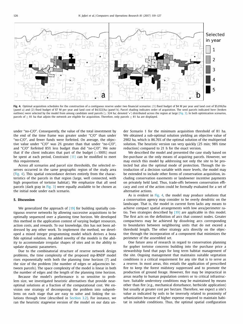
The effect of a larger budget and cheaper land on reserve design

s visually ( Fig. 4 ) and quantitatively evident ( Table 1 ) in a compar-

son of outcomes of Scenarios 1 and 2. Under the minimum acqui-

ition threshold of 81 ha, Scenario 2 returned 74% more habitat

han did Scenario 1. Under the minimum acquisition threshold of

1 ha, the corresponding comparison was almost the same (75%).

Despite equal mean annual budgets provided in Scenarios 1 and

, uncertainty in annual budget translates into an expected loss of

bjective value. The expected return under Scenario 3 was 1.9% less

han that under Scenario 1 for the minimum acquisition threshold

f 81 ha ( Table 1 ).

By expanding the solution space through relaxation of the min-

mum acquisition threshold (from 81 to 61 ha), greater values of

he objective can be achieved. For Scenarios 1 − 3 , the improve-

ent in objective value was 3%, 3%, and 2%, respectively.

However, accommodating a larger search space comes with

dded computational burden, sometimes necessitating a termina-

ion of the algorithm before an optimal solution can be achieved.

he optimality gap ( Table 1 ) measures the discrepancy between

he realized solution and the optimal solution as a percentage of

he optimal value. For both thresholds of minimum acquisition

ize, optimal solutions for Scenarios 1 and 2 were found within

wo days of run time. Similarly, optimal solutions for all cases of

cenario 3 were found within two days of run time for the mini-

um acquisition threshold of 81 ha. However, for the threshold of

1 ha, optimal solutions were not discovered in three cases of Sce-

ario 3, even after two days of run time for some cases. But in all

hree cases, the optimality gap was reasonable, ranging from 2% to

%.

The ability to carry over budget funding from one year to the

ext offers the flexibility to spend funds efficiently in the future.

iewing the spending activity on a year-by-year basis ( Table 2 ) il-

ustrates how carry-over may be exploited to obtain greater value

n future acquisitions. For example, classes “no-C/O” and “C/O”

tarted from the same initial budget amount of $4.171 M for real-

zation 1. However, under class “C/O”, less than half of that amount

as spent in the first year, and none of the accumulated amount

as spent in the second year ( Table 2 ). In doing so, larger invest-

ents were possible later in the time frame than were possible

126 N. Jafari et al. / Computers and Operations Research 81 (2017) 119–127

Fig. 4. Optimal acquisition schedules for the construction of a contiguous reserve under two financial scenarios: (1) fixed budget of $4 M per year and land cost of $5,016/ha

(panel a) and (2) fixed budget of $7 M per year and land cost of $4,522/ha (panel b). Parcel shading indicates order of acquisition. The seed parcels indicated here (broken

outlines) were selected by the model from among candidate seed parcels ( ≥ 324 ha; denoted ′ � ′ ) distributed across the region at large ( Fig. 3 ). In both optimization scenarios,

parcels of ≥ 81 ha that adjoin the network are eligible for acquisition. Therefore, only parcels ≥ 81 ha are displayed.

d

W

2

s

r

f

m

t

t

b

c

o

c

a

a

l

a

t

T

c

t

t

t

p

f

s

t

c

a

fi

p

a

t

o

b

v

u

t

under “no-C/O”. Consequently, the value of the total investment by

the end of the time frame was greater under “C/O” than under

“no-C/O”, and fewer funds were forfeited. On average, the objec-

tive value under “C/O” was 2% greater than that under “no-C/O”,

and “C/O” forfeited 85% less budget than did “no-C/O”. We note

that if the client indicates that part of the budget ( < 100%) must

be spent at each period, Constraint (11) can be modified to meet

this requirement.

Across all scenarios and parcel size thresholds, the selected re-

serves occurred in the same geographic region of the study area

( Fig. 4 ). This spatial concordance derives entirely from the charac-

teristics of the parcels in that region (large, well connected, with

high proportion of tortoise habitat). We emphasize that all seed

parcels (dark gray in Fig. 3 ) were equally available to be chosen as

the initial node under each scenario.

5. Discussion

We generalized the approach of [19] for building spatially con-

tiguous reserve networks by allowing successive acquisitions to be

optimally sequenced over a planning time horizon. We developed

this method in the application context of varying budget resources,

action costs, and rewards. To our knowledge, this has not been ad-

dressed by any other work. To implement the method, we devel-

oped a mixed integer programming model which derives a bona

fide optimal solution. An added novelty of the models is the abil-

ity to accommodate irregular shapes of sites and in the ability to

update dynamic parameters.

Due to the combinatorial structure of reserve network design

problems, the time complexity of the proposed mp-RNDP model

rises exponentially with both the planning time horizon ( T ) and

the size of the problem (the number of edges or adjacencies be-

tween parcels). The space complexity of the model is linear in both

the number of edges and the length of the planning time horizon.

Because the model’s performance is so sensitive to prob-

lem size, we investigated heuristic alternatives that provide near-

optimal solutions at a fraction of the computational cost. We en-

vision one strategy of decomposing the problem into subprob-

lems on each stage that are easy to solve and linking the so-

lutions through time (described in Section 3.2 ). For instance, we

ran the heuristic stagewise version of the model on our data un-

er Scenario 1 for the minimum acquisition threshold of 81 ha.

e obtained a sub-optimal solution yielding an objective value of

902 ha, which is 86.76% of the optimal solution of the multiperiod

olution. The heuristic version ran very quickly (25 min; 98% time

eduction) compared to 21 h for the exact version.

We described the model and presented the case study based on

ee-purchase as the only means of acquiring parcels. However, we

ay enrich this model by addressing not only the site to be pro-

ected but also the optimal mode of protection. Through the in-

roduction of a decision variable with more levels, the model may

e extended to include other forms of conservation acquisition, in-

luding conservation easements or landowner incentive payments

n privately held land. Thus, trade-offs between conservation effi-

acy and cost of the action could be formally evaluated for a set of

lternative actions.

As is evident in Fig. 4 , the model may produce solutions that

conservation agency may consider to be overly dendritic on the

andscape. That is, the model in current form lacks any means to

chieve compact spatial arrangements with low area/perimeter ra-

io. Two strategies described by [19] are applicable in this model.

he first acts on the definition of arcs that connect nodes. Greater

ompactness may be achieved by dissolving arcs corresponding

o boundaries between neighboring units that do not exceed a

hreshold length. The other strategy acts directly on the objec-

ive through the incorporation of a component that minimizes the

erimeter of the assembled set.

One future area of research in regard to conservation planning

or gopher tortoise concerns building into the purchase price a

tewardship fund that pays for long term habitat management of

he site. Ongoing management that maintains suitable vegetation

onditions is a critical requirement for any site that is to serve as

reserve. In most areas, this entails the application of prescribed

re to keep the forest midstory suppressed and to promote the

roduction of ground forage. However, fire may be impractical in

reas nearby to human population centers or to critical infrastruc-

ure. Suitable understory conditions may be maintained by means

ther than fire (e.g., mechanical disturbance, herbicide application)

ut usually at greater cost per hectare. Therefore, we expect a site’s

alue as indicated by soils to be inversely related to proximity of

rbanization because of higher expense required to maintain habi-

at in suitable conditions. Thus, the optimal spatial configuration

N. Jafari et al. / Computers and Operations Research 81 (2017) 119–127 127

o

t

p

A

f

s

S

S

R

G

U

o

N

o

a

R

[

[

[

[

[

[

[

[

[

[

[

[

[

[

[

[

[

[

[

f a reserve on a human-populated landscape should be expected

o be sensitive to whether management costs are accounted for in

urchase price.

cknowledgments

We thank Angela Fuller for a review of the manuscript and

or suggestions that improved the work. This project was spon-

ored by the U.S. Department of the Interior, Southeast Climate

cience Center and the U.S. Geological Survey Southeast Ecological

cience Center through the Georgia Cooperative Fish and Wildlife

esearch Unit, (Research Work Order 115, Cooperative Agreement

13AC00230). The Georgia Cooperative Fish and Wildlife Research

nit is jointly sponsored by U.S. Geological Survey, the University

f Georgia, U.S. Fish and Wildlife Service, Georgia Department of

atural Resources, and the Wildlife Management Institute. Any use

f trade, firm, or product names is for descriptive purposes only

nd does not imply endorsement by the U.S. Government.

eferences

[1] Armsworth PR , Daily GC , Kareiva P , Sanchirico JN . Land market feedbacks canundermine biodiversity conservation. Proc Natl Acad Sci 2006;103:5403–8 .

[2] Ashton KG , Engelhardt BM , Branciforte BS . Gopher tortoise ( Gopherus polyphe-mus ) abundance and distribution after prescribed fire reintroduction to Florida

scrub and sandhill at Archbold Biological Station. J Herpetol 2008;42:523–9 . [3] Auffenber g W , Franz R . The status and distribution of the gopher tortoise ( Go-

pherus polyphemus ). In: Bury RB, editor. North American tortoises: conserva-tion and ecology; 1982. p. 95–126 .

[4] Billionnet A . Mathematical optimization ideas for biodiversity conservation.

Eur J Oper Res 2013;231:514–34 . [5] Billionnet A . Designing robust nature reserves under uncertain survival proba-

bilities. Environ Model Assess 2014:1–15 . [6] Butsic V , Lewis DJ , Radeloff VC . Reserve selection with land market feedbacks.

J Environ Manage 2013;114:276–84 . [7] Camacho-Collados M , Liberatore F , Angulo J . A multi-criteria police districting

problem for the efficient and effective design of patrol sector. Eur J Oper Res

2015;246:674–84 . [8] Caro F , Shirabe T , Guignard M , Weintraub A . School redistricting: embedding

gis tools with integer programming. Oper Res Soc 2004;55:836–49 . [9] Carvajal R , Constantino M , Goycoolea M , Vielma JP , Weintraub A . Imposing

connectivity constraints in forest planning models. Oper Res 2013;61:824–36 . [10] Conrad JM , Gomes CP , van Hoeve WJ , Sabharwal A , Suter JF . Wildlife corridors

as a connected subgraph problem. J Environ Econ Manage 2012;63:1–18 .

[11] Contreras I , Fernndez E . General network design: a unified view of combinedlocation and network design problems. Eur J Oper Res 2012;219:680–97 .

[12] Costa A , Ramakrishnan M , Taylor P . A distributed approach to capacity alloca-tion in logical networks. Eur J Oper Res 2010;203:737–48 .

[13] Costello C , Polasky S . Dynamic reserve site selection. Resour Energy Econ2004;26:157–74 .

[14] Dilkina B , Gomes CP . Solving connected subgraph problems in wildlife con-

servation. In: International conference on integration of AI and OR techniquesin constraint programming for combinatorial optimization problems; 2010.

p. 102–16 . [15] Dissanayake ST , Önal H . Amenity driven price effects and conservation re-

serve site selection: a dynamic linear integer programming approach. EcolEcon 2011;70:2225–35 .

[16] Garfinkel RS , Nemhauser GL . Optimal political districting by implicit enumera-

tion techniques. Manage Sci 1970;16:B495–508 . [17] Haight RG , Snyder SA , Revelle CS . Metropolitan open-space protection with un-

certain site availability. Conserv Biol 2005;19:327–37 . [18] Harrison P , Spring D , MacKenzie M , Nally RM . Dynamic reserve design with

the union-find algorithm. Ecol Modell 2008;215:369–76 . [19] Jafari N , Hearne J . A new method to solve the fully connected reserve network

design problem. Eur J Oper Res 2013;231:202–9 .

20] Jantke K , Schneider U . Integrating land market feedbacks into conserva-tion planninga mathematical programming approach. Environ Model Assess

2011;16:227–38 . [21] Lunday BJ , Sherali HD , Lunday KE . The coastal seaspace patrol sector design

and allocation problem. Comput Manage Sci 2012;9:483–514 . 22] Marlin PG . Application of the transportation model to a large-scale districting

problem. Comput Oper Res 1981;8:83–96 . 23] Meir E , Andelman S , Possingham HP . Does conservation planning matter in a

dynamic and uncertain world? Ecol Lett 2004;7:615–22 .

[24] Moilanen A , Cabeza M . Accounting for habitat loss rates in sequential reserveselection: simple methods for large problems. Biol Conserv 2007;136:470–82 .

25] Mushinsky HR , McCoy ED , Wilson DS . Patterns of gopher tortoise demogra-phy in Florida. In: Proceedings of the international conference of conservation,

restoration, and management of tortoises and turtles. New York turtle and tor-toise society and WCS turtle recovery program.; 1997. p. 252–8 .

26] Naidoo R , Balmford A , Ferraro PJ , Polasky S , Ricketts TH , Rouget M . Integrating

economic costs into conservation planning. Trends Ecol Evol 2006;21:681–7 . [27] Nicholson E , Possingham HP . Making conservation decisions under uncertainty

for the persistence of multiple species. Ecol Appl 2007;17:251–65 . 28] NRCS (2016 (accessed January 5, 2016)). [natural resources conservation

service], soil survey staff, U.S. department of agriculture. [online:] http://websoilsurvey.nrcs.usda.gov/ .

29] Önal H , Briers R . Designing a conservation reserve network with minimal

fragmentation: a linear integer programming approach. Environ Model Assess2005;10:193–202 .

30] Önal H , Briers RA . Optimal selection of a connected reserve network. Oper Res2006;54:379–88 .

[31] Önal H , Wang Y . A graph theory approach for designing conservation reservenetworks with minimal fragmentation. Networks 2008;51:142–52 .

32] Possingham H , Day J , Goldfinch M , Salzborn F . The mathematics of design-

ing a network of protected areas for conservation. In: Sutton DJ, Cousins CEM,Cousins EA, editors. Proceedings of the 12th Australian operations research

conference; 1993. p. 536–45 . [33] Powell WB . Approximate dynamic programming: solving the curses of dimen-

sionality. Wiley; 2011 . 34] Rodrigues AM , Ferreira JS . Measures in sectorization problems. In: Operations

research and big data; 2015. p. 203–11 .

[35] Sabbadin R , Spring D , Rabier CE . Dynamic reserve site selection under conta-gion risk of deforestation. Ecol Modell 2007;201:75–81 .

36] Sheldon D , Dilkina B , Elmachtoub A , Finseth R , Sabharwal A , Conrad J ,Gomes C , Shmoys D , Allen W , Amundsen O , Vaughan B . Maximizing the spread

of cascades using network design. UAI: conference in uncertainty in artificialintelligence; 2010 .

[37] Shirabe T . A model of contiguity for spatial unit allocation. Geogr Anal

2005;37:2–16 . 38] Snyder S , Haight R , ReVelle C . A scenario optimization model for dynamic re-

serve site selection. Environ Model Assess 2004;9:179–87 . 39] Strange N , Thorsen B , Bladt J . Optimal reserve selection in a dynamic world.

Biol Conserv 2006;131:33–41 . 40] Sutherland C , Fuller AK , Royle JA . Modelling non-Euclidean movement and

landscape connectivity in highly structured ecological networks. Methods EcolEvol 2015;6:169–77 .

[41] Toth SF , Haight RG , Rogers LW . Dynamic reserve selection: optimal land reten-

tion with land-price feedbacks. Oper Res 2011;59:1059–78 . 42] USFWS . [U.S. fish and wildlife service], endangered and threatened wildlife and

plants; determination of threatened status for the gopher tortoise ( Gopheruspolyphemus ). Fed Regist 1987;52(129):25376–80 .

43] USFWS , NRCS . [U.S. fish and wildlife service and natural resources conservationservice], gopher tortoise ( Gopherus polyphemus ) soil classifications for the fed-

erally listed range using the national soil information system database. Tech-

nical report; 2012 . Unpublished report 44] Vansteenwegen P , Souffriau W , Oudheusden DV . The orienteering problem: a

survey. Eur J Oper Res 2011;209:1–10 . 45] Visconti P , Pressey RL , Segan DB , Wintle BA . Conservation planning with dy-

namic threats: the role of spatial design and priority setting for species per-sistence. Biol Conserv 2010;143:756–67 .

46] Williams JC . A zero-one programming model for contiguous land acquisition.

Geographical analysis. Geogr Anal 2002;34:330–49 . [47] Williams JC , ReVelle C , Levin S . Spatial attributes and reserve design models:

a review. Environ Model Assess 2005;10:163–81 .