Computers & Graphics (2018)

Contents lists available at ScienceDirect

Computers & Graphics

journal homepage: www.elsevier.com/locate/results-in-physics

3D Shape Segmentation via Shape Fully Convolutional Networks

Pengyu Wanga,∗, Yuan Gana,∗, Panpan Shuia, Fenggen Yua, Yan Zhanga, Songle Chenb, Zhengxing Suna

aState Key Lab for Novel Software Technology, Nanjing UniversitybKey Lab of Broadband Wireless Communication and Sensor Network Technology of Ministry of Education, Nanjing University of Posts and Telecommunications

A B S T R A C T

We design a novel fully convolutional network architecture for shapes, denoted by Shape Fully Convolutional Networks (SFCN).3D shapes are represented as graph structures in the SFCN architecture, based on novel graph convolution and pooling operations,which are similar to convolution and pooling operations used on images. Meanwhile, to build our SFCN architecture in the originalimage segmentation fully convolutional network (FCN) architecture, we also design and implement a generating operation withbridging function. This ensures that the convolution and pooling operation we have designed can be successfully applied in theoriginal FCN architecture. In this paper, we also present a new shape segmentation approach based on SFCN. Furthermore, weallow more general and challenging input, such as mixed datasets of different categories of shapes which can prove the abilityof our generalisation. In our approach, SFCNs are trained triangles-to-triangles by using three low-level geometric features asinput. Finally, the feature voting-based multi-label graph cuts is adopted to optimise the segmentation results obtained by SFCNprediction. The experiment results show that our method can effectively learn and predict mixed shape datasets of either similar ordifferent characteristics, and achieve excellent segmentation results.

1. Introduction

Shape segmentation aims to divide a 3D shape into meaning-ful parts, and to reveal its internal structure. This is the basis andprerequisite to explore the inherent characteristics of the shape.The results obtained from shape segmentation can be applied tovarious fields of computer graphics, such as shape editing [1],deformation [2], and modelling [3]. Shape segmentation, there-fore, has become a research hotspot, yet difficulties in the fieldsof digital geometric model processing and instance modellingpersist.

Convolutional networks have shown excellent performancein various image processing problems, such as image classifi-cation [4, 5, 6], and semantic segmentation [7, 8, 9]. With theemerging encouraging study results, many researchers have de-voted their efforts to various deformation studies on CNNs, oneof which is the fully convolutional network (FCN) [10]. Thismethod can train end-to-end, pixels-to-pixels on semantic seg-mentation, with no requirement over the size of the input image.Thus, it has become one of the key research topics in CNN net-works.

∗Equal contribution.

Although FCNs can generate good results in image segmen-tation, we cannot directly apply it to 3D shape segmentation.This is mainly because image is a type of a static 2D array,which has a very standard data structure and regular neighbour-hood relations. Therefore, convolution and pooling can be eas-ily operated when processing FCNs. However, the data struc-ture of a 3D shape is irregular, so it cannot be directly repre-sented as the data structure of an image. As triangle mesheshave no regular neighbourhood relations like image pixels, di-rect convolution and pooling operations on a 3D shape is diffi-cult to fulfil.

Inspired by the FCN architecture in image segmentation, wedesign and implement a new FCN architecture that operates di-rectly on 3D shapes by coverting a 3D shape into a graph struc-ture. Based on the FCN process of convolution and poolingoperation on the image and existing methods of Graph Convo-lutional Neural Networks [11, 12, 13], we design a shape con-volution and pooling operation, which can be applied directlyto the 3D shape. Combined with the original FCN architecture,we build a new shape fully convolutional network architectureand name it Shape Fully Convolutional Network (SFCN). Sec-ondly, following the SFCN architecture mentioned above andthe basic flow of image segmentation of FCN [10], we devise

arX

iv:1

702.

0867

5v3

[cs

.CV

] 2

6 M

ay 2

018

2 / Computers & Graphics (2018)

Fig. 1: Example of our shape segmentation results on one mixed shape dataset. The shapes on the left are part of the training set, and some segmentation results areshown on the right.

a novel trained triangles-to-triangles model for shape segmen-tation. Thirdly, for higher accuracy of segmentation, we usethe multiple features of the shape to complete the training onthe SFCN. Utilising the complementarity between features, andcombined with the multi-label graph cuts method [14, 15, 16],we optimise the segmentation results obtained by the SFCNprediction, through which the final shape segmentation resultsare obtained. Our approach can realize the triangles-to-triangleslearning and prediction with no requirements on the trianglenumbers of the input shape. Furthermore, many experimentsshow that our segmentation results perform better than those ofexisting methods [17, 18, 19], especially when dealing with alarge dataset. Finally, our method permits mixed dataset learn-ing and prediction. Datasets of different categories are com-bined together in the test, and the accuracy of the segmentationresults of different shapes decreases very little. As shown inFigure 1, for a mixed shape dataset from COSEG [20] with sev-eral categories of shapes, part of the training set are displayedon the left, and some corresponding segmentation results areshown on the right. Figure 2 shows the process of our method.

Fig. 2: The pipeline of our method. It may be divided into 3 stages: training pro-cess, using the SFCN architecture to train under three different features; testingprocess, predicting the test sets through the SFCN architecture; optimisationprocess, optimising the segmentation results by the voting-based multi-labelgraph cuts method to obtain the final segmentation results.

The main contributions of this paper include:

1. We design a fully convolutional network architecturefor shapes, named Shape Fully Convolutional Network(SFCN), and is able to achieve effective convolution andpooling operations on the 3D shapes.

2. We present the shape segmentation and labelling based onSFCN. It can be triangles-to-triangles by three low-levelgeometric features, and outperforms the state-of-the-artshape segmentation.

3. Excellent segmentation results on training and predict-ing mixed datasets of different categories of shapes areachieved.

2. Related Work

Fully convolutional networks. The fully convolutional net-work [10] proposed in 2015 is pioneering research which caneffectively solve the problem of semantic image segmentationby pixel-level classification. Later, a great deal of research hasemerged based on the FCN algorithms and achieved good re-sults in various fields such as edge detection [21], depth regres-sion [22], optical flow [23], simplifying sketches [24] and soon. However, the existing research on FCN is mainly restrictedto image processing, largely because image has a standard datastructure, easy for convolution, pooling and other operations.

Graphs CNN. Standard CNN cannot work directly on datawhich have graph structures. However, there are some previ-ous works [25, 26, 12, 13] that discuss how to train CNN ongraphs. These works [25, 13] use a spectral method by comput-ing bases of the graph Laplacian matrix, and perform the con-volution in the spectral domain. [12] use a PATCHY-SAN ar-chitecture which maps from a graph representation onto a vec-tor space representation by extracting locally connected regionsfrom graphs.

Deep learning on 3D shapes. Recent works introduce var-ious methods of deep architectures for 3D shapes. By usingvolumetric representation [27, 28], standard CNN 2d convolu-tion and pooling methods can be easily extended to 3D con-volution and pooling. However, it leads to some problemswhich cannot be completely solved, such as data sparsity andthe computation cost of 3D convolution. [29] proposed multi-view image-based Fully Convolutional Networks (FCNs) andsurface-based CRFs to do the 3D mesh labelling by using RGB-D data as input. However, it may need a lot of time to compute

/ Computers & Graphics (2018) 3

the surface-pixel reference, and more viewpoints to maximallycover the shape surface. These methods [30, 31] proposed dif-ferent deep architectures which can be trained directly on pointclouds to achieve points segmentation and other 3D points anal-ysis. However, the point cloud structure sampled from the ori-gin meshes may lack the intrinsic structure of the meshes. Forbetter understanding the intrinsic structures, many works di-rectly adapt neural networks to meshes. The first mesh CNNmethod GCNN[32] used convolution filters in local geodesicpolar coordinates. ACNN[33] used anisotropic heat kernels asfilters. MoNet[34] considered a more generalized CNN archi-tectures by using mixture model. [35] using a global seamlessparameterization for which the convolution operator is well de-fined but can only be used on sphere-like meshes. As [36, 37]show that intrinsic CNN methods can achieve better result onshape correspondence and descriptor learning with less trainingdata. More details of these techniques can be found in [38].

Supervised methods for segmentation and labelling.When using the supervised method to train a collection of la-belled 3D shapes, an advanced machine learning approach isused to complete the related training [17, 18, 19, 20, 39]. Forexample, [17] used Conditional Random Fields (CRF) to modeland learn the sample example, in order to realize the compo-nent segmentation and labelling of 3D mesh shapes. [39] firstprojected 3D shapes to 2D space, and the labelling results in2D space were then projected back to 3D shapes for mesh la-belling. [19] use Extreme Learning Machines (ELM), whichcan be used to achieve consistent segmentation for unknownshapes. [18, 29] applied deep architectures to produce the meshsegmentation.

Unsupervised segmentation and labelling. A lot of re-search methods can build a segmentation model [40, 41, 42, 43,44] and achieve joint segmentation without any label informa-tion. There are predominantly two unsupervised learning meth-ods: matching and clustering. Using the matching method, thematching relation between pair 3D shapes is obtained based onthe similarity of a relative unit given by correlation calculation.The segmentation shape of matching shape is then establishedto realize the joint segmentation [45, 40] of 3D shapes. By con-trast, clustering methods analyze all the 3D shapes in the modelset and cluster the consistent correlation units of 3D shapes intothe same class. A segmentation model is then obtained and ap-plied to consistent segmentation [42, 43, 44].

3. Shape Fully Convolution Network

In the process of image semantic segmentation, it is mainlythrough operations such as convolution and pooling that fullyconvolution network architecture completes the image segmen-tation [10]. As analyzed above, the regular data structureamongst the pixels of the image makes it easy to implementthese operations. By analogy with images, triangles of the 3Dshape can be seen as pixels on the image, but unlike pixels,triangles of the shape have no ordered sequence rules. Figure3(a) represents the regular pixels on the image, while Figure3(b) represents the irregular triangles on the shape. It is difficultto complete the convolution and pooling operation on the 3D

shape like that of the image. Therefore, based on the character-istics of 3D shape data structure and analogous to the operationon the image, we need to design a new shape convolution andpooling operation.

(a) (b) (c)

Fig. 3: Representation of different forms of data. (a) Image data representation;(b) Shape data representation; (c) Shape data represented as graph structure.

As a 3D shape is mainly composed of triangles and the con-nections among them, we can use graph structure to describe it.Each 3D shape can be represented as G = (V, E), with vertexv ∈ V for a triangle and edge e ∈ E ⊂ V × V for the con-nection of adjacent triangles. The small triangle shown in 3(b)corresponds to the graph structure shown in Figure 3(c). Basedon the graph structure, we design and implement a shape con-volution and pooling operation, which will be detailed in thefollowing section.

3.1. Convolution on ShapeConvolution is one of the two key operations in the FCN ar-

chitecture, allowing for locally receptive features to be high-lighted in the input image. When convolution is applied to im-ages, a receptive field (a square grid) moves over each imagewith a particular step size. The receptive field reads the fea-ture values of the pixels for each channel once, and a patch ofvalues is created for each channel. Since the pixels of an im-age have an implicit arrangement, a spatial order, the receptivefields always move from left to right and top to bottom. Anal-ogous to the convolution operation on the image, therefore, weneed to focus on the following two key ideas when employingconvolution operation on the shapes:

1. Determining the neighbourhood sets around each trianglefor the convolution operation according to the size of thereceptive field.

2. Determining the order of execution of the convolution op-eration on each neighbourhood set.

For the first point, the convolution operation on the image ismainly based on the neighbourhood relationship between pix-els. Accordingly, we need to construct locally connected neigh-bourhoods from the input shape. These neighbourhoods aregenerated efficiently and serve as the receptive fields of a convo-lutional architecture, permitting the architecture to learn shaperepresentations effectively.

Shape has a neighbourhood relationship just like an image,but its irregularity restrains it to be directly represented and ap-plied to the FCN learning. Yet when expressed as graph struc-tures, the locally connected neighbourhoods of each triangle ofthe shape can be easily determined with various search strate-gies. In this paper, each triangle of the shape is viewed as

4 / Computers & Graphics (2018)

Fig. 4: Convolution process on a shape. (a) Shape represented as a graph; (b) The neighbourhood nodes of different source nodes searched by a breadth-first search,among which 4, 6, 7 represent source nodes. The areas circled by orange, red and green dotted lines are the neighbourhood nodes searched by each source node. (c)Convolution order of each neighbourhood set. The ellipsis is for other neighbourhood sets not represented.

a source node. We use the breadth-first search to expand itsneighbourhood nodes on the constructed graph so as to obtainthe neighbourhood sets of each triangle in the shape. Supposethe receptive field is set as K, the size of the neighbourhood setwill be the same, including K − 1 neighbourhood nodes and asource node, all of which will be used for a follow-up convo-lution operation. Figure 4(a) shows the graph structure of theshape, while Figure 4(b) shows the neighbourhood sets of eachsource node (that is, each triangle on the 3D shape) we obtainedwith the method outlined above.

As for the second point, when performing the convolutionoperation on the image, it is easy to determine the order of theconvolution operation according to the spatial arrangement ofthe pixels. However, it is rather difficult to determine the spa-tial orders among triangles on the 3D shape. A new strategyis thus needed to reasonably sort the elements in the neigh-bourhood sets. Sorting is to ensure that the elements in eachneighbourhood set can be convolved by the same rules, so thatthe convolution operation can better activate features. For eachnode, all nodes in its neighbourhood set can be sorted by featuresimilarity (L2 similarity in the input feature space). Using thismethod, we can not only determine the order of the convolutionoperation of each neighbourhood set, but also ensure that thenodes in different sets have the same contribution regularity totheir own source nodes in the convolution operation. The finalconvolution order for each neighbourhood set is shown in Fig-ure 4(c). As shown in Figure 4(b), the execution order of theconvolution operation of the neighbourhood set obtained fromthe source node is determined by calculating the input featuresimilarity.

3.2. Pooling on Shape

Pooling is the other key operation in the FCN architecture.The pooling operation is utilised to compress the resolution ofeach feature map (the result of the convolution operation) inthe spatial dimensions, leaving the number of feature maps un-changed. Applying a pooling operation across a feature mapenables the algorithm to handle a growing number of featuremaps and generalises the feature maps by resolution reduction.Common pooling operations are those of taking the average andmaximum of receptive fields over the input map [11]. We share

the same pooling operation on shape fully convolutional net-works with the operation mentioned above. However, we needto address a key concern; that is, to determine the pooling op-erating order of the SFCN on the shape feature map.

Similar to the convolution operation, we cannot directly de-termine the pooling operation order on SFCN based on spatialrelationships among the triangles of the 3D shape. Since the3D shape has been expressed as a graph structure, we can de-termine the pooling operation order according to the operationof convolutional neural networks on the graph. In this paper,the pooling operation on the SFCN is computed by adoptingthe fast pooling of graphs [12, 13].

The pooling method for graphs [12, 13] coarsens the graphwith the Graclus multi-level clustering algorithm [46]. Graphcoarsening aims to determine the new structure of the graphafter pooling. We first present each shape as a graph struc-ture, then we exploit the feature information on the trianglesof the shape and the Graclus multi-level clustering algorithm[46] to complete shape coarsening; that is, to determine the newconnection relationship of the shape feature map after pooling,which is shown in Figure 5(a).

In the pooling process, traversing the feature map in a cer-tain order according to the size of the receptive field is a keystep to complete the calculation, namely, to determine the oper-ation order of pooling. Following the method of pooling for thegraph proposed by [13], the vertices of the input graph and itscoarsened versions are irregularly arranged after graph coars-ening. To define the pooling order, therefore, a balanced binarytree is built by adding fake code to sort the vertices. Lastly,the pooling operation of the graph is completed based on thenodes order and the use of a 1D signal pooling method. Af-ter shape coarsening, we apply the same approach in this studyto determine the order of pooling operations on the shape fullyconvolutional networks architecture, as shown in Figure 5(b).

4. Shape Segmentation via Shape Fully Convolution Net-work

We design a novel shape segmentation method based onSFCN, analogous to the basic process of image semantic seg-mentation on FCN [10]. Firstly, we extract three categoriesof commonly used geometric features of the shape as an in-

/ Computers & Graphics (2018) 5

Fig. 5: Example of graph coarsening and pooling. (a) Graph coarsening process. Note: the original graph has 9 arbitrarily ordered vertices. For a pooling of size4, two coarsenings of size 2 are needed. To ensure that in the coarsening process the balanced binary tree can be constructed, we need to add appropriate fakenodes through calculation, which are identified in red. After coarsening, the node order on G3 is still arbitrary, yet it can be manually set. Then backstepping thecoarsening process, we can determine the node order of G2 and G1, and the corresponding relationship between nodes in each layer according to the order of G3. Atthat point the arrangement of vertices in G1 permits a regular 1D pooling. (b) Pooling order. The nodes in the first layer (blue and red) represent the G1 node order;the second layer (yellow and red) represents G2 node order; the third layer (purple) represents the G3 node order and the corresponding relationship between nodesin each layer. The red nodes are fake nodes, which are set to 0 in the pooling process, as we carry out maximum pooling.

put for SFCN training and learning. Secondly, based on theshape convolution and pooling operation proposed in Section 3and the basic process of image semantic segmentation on FCN,we design a lattice structure suitable for 3D shape segmenta-tion. Through training and learning of the network, we producetriangles-to-triangles labelling prediction. Finally, we introducethe optimisation process of shape segmentation.

4.1. Geometric Feature Extraction

Our approach is designed to complete the network trainingand learning based on some common and effective low-levelfeatures. In this paper, therefore, we extract three from the ex-isting commonly used ones as the main features for the net-work training and learning. The three features include: averagegeodesic distance (AGD) [47], shape context (SC) [48] and spinimage (SI) [49]. These features describe the characteristics ofeach triangle on a shape from multiple perspectives well. Wealso found in the experiment that these three features are com-plementary, which will be analyzed in detail in the experimentalpart.

4.2. Shape Segmentation Networks Structure

As the convolution and pooling operations on a shape are dif-ferent from those on an image, the FCN architecture originallyused in image segmentation cannot be directly applied on the3D shape. We modify the original FCN architecture accordingto the convolution and pooling characteristics, so that it can beconducted in shape segmentation.

Our training network is made up of four parts: convolution,pooling, generating and deconvolution layers, as shown in Fig-ure 7. The convolution layer corresponds to a feature extrac-tor that transforms the input shape to multidimensional featurerepresentation. The convolution operation is completed by themethod proposed in section 3.1. The pooling layer is used to

reduce the feature vector of the convolution layer, and expandits receptive field to integrate feature points in the small neigh-bourhood into the new ones as output. The pooling operation iscompleted by the method proposed in section 3.2.

As our convolution and pooling operations are designed forshapes, the original FCN architecture cannot be used directly.Compared with the original FCN’s architecture, the architectureof the SFCN in this paper needs to record every neighbourhoodset of each shape that participated in the convolution obtained inSection 3, as well as the convolution and pooling order of eachshape. Thus, we add a generating layer in the original FCNarchitecture, whose diagram of concrete meaning is shown inFigure 6.

Fig. 6: Diagram of the generating layer. (a) The pooling order. A red numberrepresents the offset, nodes in the blue circles represent nodes on the graph,nodes in the red circles are fake nodes. (b) Recorded neighbourhood set of eachnode. The numbers in the table represent the offset of each node after poolingsorting. (c) Data storage of the generating layer proposed in this paper, basedon which our method can implement convolution operation by row and poolingoperation by column.

6 / Computers & Graphics (2018)

Fig. 7: The SFCN architecture we designed, mainly including 4 parts: convolution, pooling, generating, and deconvolution layers, which are represented by gen,con, pool and deconv respectively. Additionally, fully stands for fully connectivity and the numerical values reflect the dimension changes of each layer aftercalculation. C represents feature dimension, h represents the number of triangles of each shape and n represents the shape segmentation labels.

Firstly, as shown in Figure 6(a), we can calculate the poolingorder between nodes of the graph by the shape pooling methodproposed in Section 3.2 (these nodes are equivalent to the tri-angle of the shape). We store the nodes in the calculation orderon the generating layer, as shown in Figure 6(c). Figure 6(a)gives the pooling order on a shape, where the figures representthe number of nodes (i.e. triangles).

Secondly, we need to record the neighbourhood sets of eachnode (i.e. each triangle of the shape) involved in the convolu-tion computation, as shown in Figure 6(b), where we store theneighbourhood sets by reading the offset in Figure 6(a). Af-ter the nodes are sorted by column on the generating layer, werecord their neighbourhood sets, in which the nodes are sortedaccording to the convolution order calculated in Section 3.1. Asshown in Figure 6(c), each row that is sequenced in the convo-lution order represents a neighbourhood set of a node, wherethe figures represent the number of nodes (i.e. triangles). Bystoring the data in this way, we can achieve the convolution op-eration by row and the pooling operation by column, as shownin Figure 6(c). Another advantage of such storage is that, afterpooling, the new neighbourhood set and the pooling order re-quired by the next convolution layer of each new node can stillbe obtained and be applied to the next generating layer usingthe method in Section 3.2.

The deconvolution layer can be used to perform upsamplingand densify our graph representation. As mention above, weregard pooling as a graph coarsening by clustering 4 vertices,as shown in Figure7. Conversely, the upsampling operation canbe regarded as a reverse process of the graph coarsening. Werecord how vertices are being matched before and after graphcoarsening. Therefore it is easy to reuse the efficient deconvo-lution implementation based on the image-based FCN[10]. Inthis paper, the width of the convolution kernel in the deconvo-lution layer of the original FCN architecture is changed to 1

and the height is set to the size of the pooling we use, therebyobtaining the deconvolution layer of SFCN. The final output ofthe layer is a probability map, indicating the probability of eachtriangle on a shape that belongs to one of the predefined classes.

Based on the FCN architecture proposed by [10], we designan SFCN architecture suitable for shape segmentation. Ourconvolution has five convolutional layers altogether, with eachconvolution layer having a generating layer before generatingdata for the next convolution and pooling, and followed by apooling layer. Two fully connected layers are augmented atthe end to impose class-specific projection. Corresponding tothe pooling layer, there are five deconvolution layers, throughwhich we can obtain the prediction probability of each trian-gle of the shape that belongs to each class. In the predictionprocess, we used the same skip architecture [10]. It can com-bine segmentation information from a deep, coarse layer withappearance information from a shallow, fine layer to produceaccurate and detailed segmentations as the original FCN archi-tecture. The specific process is shown in Figure 8. The pre-diction probability of each layer can be obtained by adding theresults of a deconvolution layer and the corresponding resultsof the pooling layer after convolution, which also functions asthe input for the next deconvolution layer. The number of rowswill be repeated 5 times to return to the initial number of trian-gles, where the value of each channel is the probability of thisclass, realizing the triangle level prediction. Another differencefrom the original FCN architecture is that, in order to normalisethe data, we add a batch normalisation layer after the convolu-tion operation of the first layer of the original FCN architecture,using the default implementation of the BN in the Caffe [50].

4.3. Shape Segmentation OptimisationWe train these three features separately using the network

structure provided in Section 4.2. Given testing shapes, theSFCN produces the corresponding segmentation results under

/ Computers & Graphics (2018) 7

Fig. 8: The skip architecture for prediction. Our DAG nets learn to combine the coarse, high layer information with the fine, low layer one. We get the predictionresults of the final layer by upsampling the score, then upsample again the prediction results combined with the final layer and the pool4 layer. After upsampling5 times, we obtain the final prediction results, combining the final layer, pool5, pool4, pool3, pool2 and pool1 layer information, which then achieves triangles-to-triangles prediction.

each feature, which can describe the segmentation of 3D shapesfrom different perspectives. Besides, due to the different in-put geometry features, there may be some differences amongthe predicted segmentation results of the same shape. To ob-tain the final segmentation results, we leverage the complemen-tarity among features and the multi-label graph cuts method[14, 15, 16] to optimise the segmentation results of the testingshape. The final segmentation result is obtained mainly throughthe optimisation of the following formula.

E(l) =∑uεV

ED(u, lu) +∑{u,v}εE

ES (u, v, lu, lv). (1)

In this formula, lu and lv are labels of triangles u and v, dataitem ED(u, lu) describes the energy consumption of triangle umarked as label lu, and smoothing item ES describes the energyconsumption of neighboring triangles marked using different la-bels.

The first item of the formula is optimised mainly based onthe probability that triangle u is marked as label lu. We predictthe shape under the three features respectively, so the same tri-angle u will have its own prediction probability under each fea-ture. In this paper, utilising the feature’s complementarity, wevote the labelling results to get the final prediction probability,and serve its negative logarithm similar to the paper [18] as thefirst item of the multi-label graph cut. The second item in theformula smooths the segmentation results mainly through thecalculation of the dihedral angle of the triangle and its neigh-bouring one. In this paper, the dihedral angle multiplied by theside length makes the second item of the formula to completeoptimisation. Energy E is minimized by employing Multi-labelGraph Cuts Optimisation[14, 15, 16], through which we canobtain more accurate shape segmentation results.

5. Experimental Results and Discussion

Data. In this paper, deep learning is used to segment theshape. Therefore to verify the effectiveness of this method,

we first tested 3 existing large datasets from COSEG [20], in-cluding the chair dataset of 400 shapes, the vase dataset of 300shapes and the alien dataset of 200 shapes. The experiment ofthe mixed dataset was also carried out on the Princeton Segmen-tation Benchmark (PSB) [51] dataset. In addition, to confirmthe robustness of the above method, we also selected 11 cate-gories in the PSB[51] dataset for testing, each of them contain-ing 20 shapes. For COSEG datasets, we chose the groundtruthas in the paper[20]. For PSB datasets, we chose the groundtruthas in the dissertation[17].

SFCN Parameters. We trained by SGD with momentum, us-ing momentum 0.9 and weight decay of 1e-3. We chose ReLUas the activation function. Dropout used in the original classi-fier nets is included. The per-triangle, unnormalised softmaxloss is a natural choice for segmenting shapes of any size, withwhich we trained our nets.

Computation Time. We used two Intel(R) Xeon(R) CPU E5-2620 v3 @ 2.40GHz with 12 cores and NVIDIA GeForce TI-TAN X GPU. In large datasets, when we used 50 shapes fortraining and the triangles of each shape range from 1000 to5000, the training would take approximately 120 minutes (in-cluding the time to compute the input descriptors), and the testand optimisation of a shape took about 30 seconds.

Results. In the experiment, we used the classification accu-racy proposed by Kalogerakis [17] and Sidi [41] for the quanti-tative evaluation of our method.

Firstly, to compare with the methods of [18] in the COSEG’slarge dataset, we randomly selected 50 shapes for training fromthe chair dataset and 20 shapes for training from the vase date-set. We compared our method with three shape segmentationmethods [41, 52, 18]. The results are presented in Table 1. Itshould be noted that the results and data obtained by other meth-ods come from [18]. The table shows that the results obtainedby our method outperform the existing methods, thus provingthat our method is effective.

Secondly, to verify the effectiveness of our method for largedatasets, we randomly selected 25%, 50% and 75% of the

8 / Computers & Graphics (2018)

Fig. 9: Results under Large Datasets

Table 1: Labelling Accuracy of Large Datasets.

TOG[2011]

TOG[2013]

TOG[2015]

Ours

Chair 80.20% 91.20% 92.52% 93.11%Vase 69.90% 85.60% 88.54% 88.91%

ToG[2011] is short for Sidi et al. [TOG 2011], ToG[2013] is short for Kimet al.[TOG 2013],ToG[2015] is short for Guo et al.[2015].

shapes for training from each of the three large datasets fromCOSEG. To verify whether the SFCN prediction accuracy be-comes higher as the number of training sets increases, we usedthe same 25% shapes for testing in each experiment for eachlarge dateset. In other words, the training sets gradually in-creased, while the test set remained the same. The results ofthis can be seen in Table 2. Because the work of [19] carriedout a similar experiment under a 75% training condition withtheir method, we also make a comparison with their results inTable 2. It can be seen from the table that the results obtainedby our method perform better than theirs. Furthermore, withthe increase of the training set, the classification accuracy ofour method grows steadily in the same test set. This shows thatwith the increase of the training set, both the learning abilityand the generalisation ability of the network architecture be-come stronger, which also proves the effectiveness of the de-signed network in this paper.

Table 2: Labelling Accuracy of Large Datasets. Here are the results of the sametest set for different numbers of training sets.

Ours25%

Ours50%

Ours75%

CGF[2014]75%

Chair 93.43% 94.38% 95.91% 87.09%Vase 88.04% 90.95% 91.17% 85.86%

Tele-alien 91.02% 92.76% 93.00% 83.23%

CGF[2014] is short for Xie et al.[CGF 2014]

Thirdly, we visualize the segmentation results obtained byusing our method in the three large datasets of COSEG, asshown in Figure 9. All the results shown are optimised andobtained using the 75% training set. The segmentation resultsappear visually accurate, which proves the effectiveness of thismethod.

Mixed dataset training and testing were performed as well.We respectively mixed airplane and bird, human and teddy,which are of similar classes. It must be noted that, unlike the

method of [18] which merges similar class labels, we retainedthese different labels. So the body of the plane and bird havedifferent labels; their wings as well. 12 shapes of each datasetwere selected as the training set, and the remaining as the testset. Our approach was repeated three times to compute the aver-age performance, the segmentation results of which are shownin Figure 10. Figure 10(a) is part of the result of the training setwhile Figure 10(b) is part of the testing set. The classificationaccuracy of the two datasets is shown in Table 3, which suggeststhat we can obtain good segmentation results when mixing sim-ilar data together. Although the segmentation accuracy is not ashigh as training, the average is above 90%. Additionally, the ba-sic segmentation is correct according to the visualisation of theresults, proving that SPFCN network architecture is powerful indistinguishing features and learning.

Table 3: Labelling Accuracy of Mixed Datasets of Similar Shapes

Airplane &Bird

Human &Teddy

Accuracy 90.04% 92.28%

In addition, we mixed glasses and pliers, glasses, pliers, fishand tables of different categories. From the mixed datasets, weselected some data for training, with the remaining used for test-ing. Here 12 shapes of each dataset were selected as the trainingset, and the remaining as the test set. We also mixed two largedatasets with 400 chairs and 300 vases. We selected 50% of theshapes for training from each dataset and the remaining 50% asthe test set. Our approach was repeated three times to computethe average performance, the segmentation results of which areshown in Figure 11 and Figure 1. Figure 11(a) is part of theresult of the training set while Figure 11(b) is part of the testingset. The classification accuracy of the three datasets is shown inTable 4, which also indicates that both the segmentation resultsand classification accuracy achieve impressive performance. Inother words, this method can be used to train and predict anyshape set, and proves once again that our SFCN architecturehas good feature distinguishing ability and learning ability.

Table 4: Labelling Accuracy of Mixed Datasets of Different Shapes

Glasses& Plier

Chair(400)&

Vase(300)

Glasses &Plier & Fish

& Table

Accuracy 96.53% 87.71% 91.82%

/ Computers & Graphics (2018) 9

Lastly, as in the papers of [18], we separately trained sev-eral small datasets of PSB when N = 6 and N = 12 (i.e., SB6,SB12), in which N is the number of randomly selected shapesin each training process. For each category of dataset, as inthe papers of [18], we repeated our approach five times to com-pute the average performance. The comparison results with therelated methods are presented in Table 5. It should be notedthat the results and data obtained by other methods come from[18]. As shown in Table 5, the results of several datasets ofPSB obtained by our method perform much better in most cate-gories than the existing methods [17, 18, 19, 39, 53, 54], whichproves the effectiveness of the method. On a few individualdatasets, such as airplane, chair and table etc., our results donot go beyond those of other methods, yet are very close to thebest ones, which also serves to prove that our method is effec-tive. Moreover, the segmentation effect gradually strengthens asthe training data increases, which shows that the learning abil-ity of the SFCN architecture is enhanced with the increase oftraining samples. We also visualize the segmentation results ofseveral datasets of PSB including teddy, pliers and fish etc. onthe condition of SB12, the optimised ones of which are shownin Figure 12. Just like the large dataset, the results of the smallone are visually accurate, which indicates that our method isfeasible.

Fig. 10: The Segmentation Results of Mixed Datasets of Similar Shapes. (a)Part of the shapes in the training set; (b) Segmentation results of part of theshapes in the testing set.

Fig. 11: The Segmentation Results of Mixed Datasets of Different Shapes. (a)Part of the shapes in the training set; (b) Segmentation results of part of theshapes in the testing set.

Feature sensibility. In this paper, we combine three features,average geodesic distance (AGD) [47], shape context (SC) [48]and spin image (SI) [49] to produce the shape segmentation. Toverify the validity of this combination, we carried out a compar-ative experiment. The classification accuracy of each datasetof PSB under a single feature, and the one obtained with our

Fig. 12: More results of our method.

method are compared in the condition of SB6, as shown in Fig-ure 13. It can be seen that the classification accuracy of individ-ual datasets under individual features is higher, but not signifi-cantly more so than that of our method. On the contrary, mostdatasets perform much better under our method. This showsthat the features selected in this paper are complementary andthe feature combination is effective.

Fig. 13: The Comparison of Segmentation Accuracy under Different Features

In the papers of [17] and [18], seven features are combinedto perform segmentation experiments. In addition to the threefeatures used in this paper, they also used four other features in-cluding curvature (CUR) [55], PCA feature (PCA) [56], shapediameter function (SDF) [57] and distance from medial surface(DIS) [10]. In this paper, several datasets of PSB are randomlyselected to perform experiments with the combination of sevenfeatures. Under the same experimental conditions, the compari-son results with the combination of three features are presentedin Figure 14. The experiment tells us that for most datasets, thecombination of three features brings higher classification ac-curacy than seven features, and for the remaining few datasets,the classification accuracy of the two is very close to each other.This indicates that the three features used in this paper can notonly better complement, but also are more suitable for the net-work structure. In addition, we also trained the combining threefeatures in one SFCN network. However, it didn’t produce ahigher accuracy result and nearly doubled the training time. So,as a trade-off between performance and efficiency, we empir-

10 / Computers & Graphics (2018)

Table 5: Labelling Accuracy on Princeton Benchmark(SB6/SB12)

SVMSB6

JointBoostSB6

ToG[2010]SB6

ToG[2013]SB6

ToG[2015]SB6

OursSB6

ToG[2010]SB12

ToG[2013]SB12

ToG[2015]SB12

OursSB12

Cup 94.11% 93.12% 99.1% 97.5% 99.49% 99.59% 99.60% 99.60% 99.73% 99.74%

Glasses 95.92% 93.59% 96.10% - 96.78% 97.15% 97.20% - 97.60% 97.79%

Airplane 80.43% 91.16% 95.50% - 95.56% 93.90% 96.10% - 96.67% 95.30%

Chair 81.38% 95.67% 97.80% 97.90% 97.93% 97.05% 98.40% 99.60% 98.67% 98.26%

Octopus 97.04% 96.26% 98.60% - 98.61% 98.67% 98.40% - 98.79% 98.80%

Table 90.16% 97.37% 99.10% 99.60% 99.11% 99.25% 99.30% 99.60% 99.55% 99.41%

Teddy 91.01% 85.68% 93.30% - 98.00% 98.04% 98.10% - 98.24% 98.27%

Plier 92.04% 81.55% 94.30% - 95.01% 95.71% 96.20% - 96.22% 96.55%

Fish 87.05% 90.76% 95.60% - 96.22% 95.63% 95.60% - 95.64% 95.76%

Bird 81.49% 81.80% 84.20% - 87.51% 89.03% 87.90% - 88.35% 89.48%

Mech 81.87% 75.73% 88.90% 90.20% 90.56% 91.72% 90.50% 91.30% 95.60% 96.05%

Average 88.41% 89.34% 94.77% 96.30% 95.89% 95.98% 96.12% 97.53% 96.82% 96.85%

ToG[2010] is short for Kalogerakis et al. [2010], ToG[2013] is short for Wang et al. [2013],ToG[2015] is short for Guo et al.[2015].

ically trained 3 features separately to perform a segmentationtask.

Fig. 14: The Comparison between Segmentation Accuracy under Three Fea-tures and under Seven Features

Skip architecture. During the SFCN training process, weutilised skip architecture of five layers and integrated the crosslayer information with different steps to improve the SFCN seg-mentation results, and gradually improve the segmentation de-tails. To verify the skip architecture can do mesh labellinglearning and improve the segmentation results, we visualisedthe cross-layer prediction results with different steps. The seg-mentation results of several shapes crossing one to five layersare shown in Figure 15, where (f) is the groundtruth of the cor-responding shape. Through tracking of the network computingprocess, we find that the network convergence is faster with theincrease of the cross layers. In addition, it can be seen from thecomparison results of cross layers and groundtruth in Figure 15,that with the increase of cross layers, the classification quality

is gradually improved.

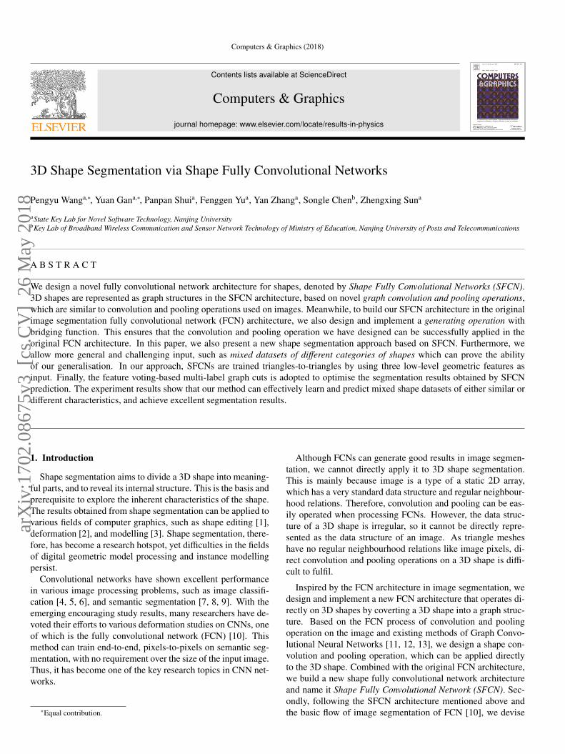
Comparison before and after optimisation. In this paper, weuse the multi-label graph cut optimisation method [14, 15, 16]to optimise the segmentation results of testing shapes, based onthe complementarity between features. The comparison resultsbefore and after optimisation of several shapes are shown inFigure 16. As shown in Figure 16(a), the results before optimi-sation are the final ones obtained by voting on the three differentfeatures tested by SFCN architecture. Figure 16(b) representsresults after optimisation. As the results before optimisation arepredicted in the triangle level, the boundary may be not smoothor there may be prediction errors of individual triangles in someareas. The above problems are well addressed after the opti-misation with the multi-label graph cuts optimisation method[14, 15, 16], which proves that optimisation plays a significantrole. In addition, the number below each figure is the classifi-cation accuracy of the corresponding shape, which shows thatoptimisation can improve classification accuracy.

Fig. 15: The Segmentation Results of Layer Information with Different Steps.(a)- (e) Segmentation results Crossing 1 to 5 layers; (f) Groundtruth.

Limitations. Although the proposed method is effective atcompleting the 3D shape segmentation task, it has some limi-tations. Firstly, the shapes involved in the calculation must bemanifold meshes, for they can easily determine the connection

/ Computers & Graphics (2018) 11

Fig. 16: Comparison Results before and after optimisation. (a) Segmentationresults before optimisation; (b) Segmentation results after optimisation. Thenumber below each shape is the segmentation accuracy.

between triangles. Secondly, the designed SFCN architecturehas no feature selection function, thus we carry on the sepa-rating training for the three features. Thirdly, to obtain betterparameter sharing, the SFCN structure may need all trainingmeshes to be the same triangulation granularity. Therefore, infuture work, we will seek to improve the SFCN architecture,making it possible for automatic feature selection, and build anend-to-end structure.

6. Conclusions

We design a novel shape fully convolutional network archi-tecture, which can automatically carry out triangles-to-triangleslearning and prediction, and complete the segmentation taskwith high quality. In the SFCN architecture proposed here,similar to convolution and pooling operation on images, we de-sign a novel shape convolution and pooling operation with a3D shape represented as a graph structure. Moreover, basedon the original image segmentation FCN architecture [10], wefirst design and implement a new generating operation, whichfunctions as a bridge to facilitate the execution of shape con-volution and pooling operations directly on 3D shapes. Ad-ditionally, accurate and detailed segmentation of 3D shapes iscompleted through skip architecture. To produce more accuratesegmentation results, we optimise the segmentation results ob-tained by SFCN prediction by utilising the complementarity be-tween the three geometric features and the multi-label graph cutmethod [14, 15, 16], which can also improve the local smooth-ness of triangle labels. The experiments show that the proposedmethod can not only obtain good segmentation results both inlarge datasets and small ones with the use of a small numberof features, but also outperform some existing state-of-the-artshape segmentation methods. More importantly, our methodcan effectively learn and predict mixed shape datasets either of

similar or of different characters, and achieve excellent segmen-tation results, which demonstrates that our method has stronggeneralisation ability.

In the future, we want to strengthen our method to overcomesome limitations mentioned above and produce more resultsbased on various challenging datasets, such as ShapeNet. Ad-ditionally, we hope that the SFCN architecture proposed canbe applied to other shape fields, such as shape synthesis, linedrawing extraction and so on.

Acknowledgements

We would like to thank all anonymous reviewers for theirconstructive comments. This research has been supportedby the National Science Foundation of China (61321491,61100110, 61272219) and the Science and Technology Pro-gram of Jiangsu Province (BY2012190, BY2013072-04).

References

[1] Yu, Y, Zhou, K, Xu, D, Shi, X, Bao, H, Guo, B, et al. Mesh editingwith poisson-based gradient field manipulation. ACM Transactions onGraphics 2004;23(3):644–651.

[2] Yang, Y, Xu, W, Guo, X, Zhou, K, Guo, B. Boundary-aware multi-domain subspace deformation. IEEE Transactions on Visualization &Computer Graphics 2013;19(19):1633–45.

[3] Chen, X, Zhou, B, Lu, F, Tan, P, Bi, L, Tan, P. Garment modelingwith a depth camera. ACM Transactions on Graphics 2015;34(6):1–12.

[4] Krizhevsky, A, Sutskever, I, Hinton, GE. Imagenet classification withdeep convolutional neural networks. Advances in Neural Information Pro-cessing Systems 2012;25(2):2012.

[5] Szegedy, C, Liu, W, Jia, Y, Sermanet, P, Reed, S, Anguelov, D, et al.Going deeper with convolutions. Proceedings of the IEEE Conference onComputer Vision and Pattern Recognition 2015;:1–9.

[6] Simonyan, K, Zisserman, A. Very deep convolutional networks forlarge-scale image recognition. Computer Science 2014;.

[7] Ciresan, D, Giusti, A, Gambardella, LM, Schmidhuber, J. Deep neuralnetworks segment neuronal membranes in electron microscopy images.In: Advances in neural information processing systems. 2012, p. 2843–2851.

[8] Farabet, C, Couprie, C, Najman, L, Lecun, Y. Learning hierarchicalfeatures for scene labeling. IEEE Transactions on Pattern Analysis &Machine Intelligence 2013;35(8):1915–29.

[9] Pinheiro, P, Collobert, R. Recurrent convolutional neural networks forscene parsing. ICML 2014;.

[10] Long, J, Shelhamer, E, Darrell, T. Fully convolutional networks forsemantic segmentation. CVPR 2015;.

[11] Edwards, M, Xie, X. Graph based convolutional neural network. BMVC2016;.

[12] Niepert, M, Ahmed, M, Kutzkov, K. Learning convolutional neuralnetworks for graphs. ICML 2016;.

[13] Defferrard, M, Bresson, X, Vandergheynst, P. Convolutional neuralnetworks on graphs with fast localized spectral filtering. NIPS 2016;.

[14] Boykov, Y, Veksler, O, Zabih, R. Efficient approximate energy mini-mization via graph cuts. IEEE Transactions on Pattern Analysis & Ma-chine Intelligence 2001;20(12):1222–1239.

[15] Kolmogorov, V, Zabih, R. What energy functions can be minimizedviagraph cuts? Pattern Analysis & Machine Intelligence IEEE Transactionson 2004;26(2):147–59.

[16] Boykov, Y, Kolmogorov, V. An experimental comparison of min-cut/max-flow algorithms for energy minimization in vision. IEEE Trans-actions on Pattern Analysis & Machine Intelligence 2004;26(9):1124–37.

[17] Kalogerakis, E, Hertzmann, A, Singh, K. Learning 3d mesh segmenta-tion and labeling. Acm Transactions on Graphics 2010;29(4):157–166.

[18] Guo, K, Zou, D, Chen, X. 3d mesh labeling via deep convolutionalneural networks. ACM Transactions on Graphics 2015;35(1):3.

12 / Computers & Graphics (2018)

[19] Xie, Z, Xu, K, Liu, L, Xiong, Y. 3d shape segmentation and labeling viaextreme learning machine. Computer Graphics Forum 2014;33(5):85–95.

[20] Wang, Y, Asafiy, S, van Kaickz, O, Zhang, H, Cohen-Or, D, Chen,B. Active co-analysis of a set of shapes. Acm Transactions on Graphics2012;31(6):157:1–157:10.

[21] Xie, S, Tu, Z. Holistically-nested edge detection. IEEE InternationalConference on Computer Vision 2015;:1395–1403.

[22] Liu, F, Shen, C, Lin, G, Reid, I. Learning depth from single monocu-lar images using deep convolutional neural fields. IEEE Transactions onPattern Analysis & Machine Intelligence 2015;38(10):1–1.

[23] Dosovitskiy, A, Fischer, P, Ilg, E, H’́ausser, P, HazrbaÅ, C, Golkov, V,et al. Flownet: Learning optical flow with convolutional networks. IEEEInternational Conference on Computer Vision & (ICCV) 2015;:2758–2766.

[24] Simo-Serra, E, Iizuka, S, Sasaki, K, Ishikawa, H. Learning to simplify:Fully convolutional networks for rough sketch cleanup. Acm Transactionson Graphics 2016;35(4):1–11.

[25] Bruna, J, Zaremba, W, Szlam, A, LeCun, Y. Spectral networks andlocally connected networks on graphs. ICLA 2014;.

[26] Duvenaudy, D, Maclauriny, D, Aguilera-Iparraguirre, J, Gomez-Bombarelli, R, Hirzel, T, Aspuru-Guzik, A, et al. Convolutional net-works on graphs for learning molecular fingerprints. In Advances in Neu-ral Information Processing Systems 2015;:2224–2232.

[27] Wu, Z, Song, S, Khosla, A, Yu, F, Zhang, L, Tang, X, et al. A deep rep-resentation for volumetric shapes. Proceedings of the IEEE Conferenceon Computer Vision and Pattern Recognition 2015;.

[28] Qi, CR, Su, H, Niener, M, Dai, A, Yan, M, Guibas, L. Volumetric andmulti-view cnns for object classification on 3d data. Computer Vision andPattern Recognition& (CVPR) 2016;.

[29] Kalogerakis, E, Averkiou, M, Maji, S, Chaudhuri, S. 3d shape segmen-tation with projective convolutional networks. Proceedings of the IEEEComputer Vision and Pattern Recognition 2017;.

[30] Yi, L, Su, H, Guo, X, Guibas, L. Syncspeccnn: Synchronized spectralcnn for 3d shape segmentation. Proceedings of the IEEE Computer Visionand Pattern Recognition 2017;.

[31] Su, H, Qi, C, Mo, K, Guibas, L. Pointnet: Deep learning on point setsfor 3d classification and segmentation. Proceedings of the IEEE Com-puter Vision and Pattern Recognition 2017;.

[32] Masci, J, Boscaini, D, Bronstein, MM, Vandergheynst, P. Geodesicconvolutional neural networks on riemannian manifolds. 3DRR 2015;.

[33] Boscaini, D, Masci, J, Rodol, E, Bronstein, MM. Learning shapecorrespondence with anisotropic convolutional neural networks. NIPS2016;.

[34] Monti, F, Boscaini, D, Masci, J, Rodol, E, Svoboda, J, Bronstein,MM. Geometric deep learning on graphs and manifolds using mixturemodel cnns. CVPR 2017;.

[35] Maron, H, Galun, M, Aigerman, N, Trope, M, Dym, N, Yumer, E,et al. Convolutional neural networks on surfaces via seamless toric covers.SIGGRAPH 2017;.

[36] Boscaini, D, Masci, J, Bronstein, MM, Castellani, U. Learning class-specific descriptors for deformable shapes using localized spectral con-volutional networks. Eurographics Symposium on Geometry Processing2015;34(5):13–23.

[37] Litany, O, Remez, T, Rodol, E, Bronstein, AM, Bronstein, MM. Deepfunctional maps: Structured prediction for dense shape correspondence.ICCV 2017;.

[38] Bronstein, MM, Bruna, J, LeCun, Y, Szlam, A, Vandergheynst, P.Geometric deep learning: going beyond euclidean data. IEEE Sig ProcMagazine 2017;.

[39] Wang, Y, Gongy, M, Wang, T, Cohen-Or, D, Zhang, H, Chen, B. Pro-jective analysis for 3d shape segmentation. Acm Transactions on Graphics2013;32(6):1–12.

[40] Huang, Q, Koltun, V, Guibas, L. Joint shape segmentation with linearprogramming. ACM Transactions on Graphics(TOG) 2011;30(6):125:1–125:12.

[41] Sidi, O, van Kaick, O, Kleiman, Y, Zhang, H, Cohen-Or, D. Unsu-pervised co-segmentation of a set of shapes via descriptor-space spectralclustering. In: SIGGRAPH Asia Conference. 2011, p. 1.

[42] Hu, R, Fan, L, Liu, L. Co-segmentation of 3d shapes via subspaceclustering. Computer Graphics Forum 2012;31(5):17031713.

[43] Meng, M, Xia, J, Luo, J, He, Y. Unsupervised co-segmentation for 3dshapes using iterative multi-label optimization. Computer-Aided Design

2013;45(2):312–320.[44] Xu, K, Li, H, Zhang, H, Cohen-Or, D, Xiong, Y, Cheng, ZQ.

Style-content separation by anisotropic part scales. Acm Transactionson Graphics 2010;29(6):184.

[45] Kreavoy, V, Julius, D, Sheffer, A. Model composition from interchange-able components. Conference on Computer Graphics & Applications2007;:129–138.

[46] Dhillon, IS, Guan, Y, Kulis, B. Weighted graph cuts without eigen-vectors: A multilevel approach. IEEE Trans Pattern Anal Mach Intell2007;29(11):1944–1957.

[47] Hilaga, M, Shinagawa, Y, Kohmura, T, Kunii, TL. Topology matchingfor fully automatic similarity estimation of 3d shapes. In: Conference onComputer Graphics and Interactive Techniques. 2001, p. 203–212.

[48] Belongie, S, Malik, J, Puzicha, J. Shape matching and object recognitionusing shape contexts. IEEE Transactions on Pattern Analysis & MachineIntelligence 2002;24(4):509–522.

[49] Johnson, AE, Hebert, M. Using spin images for efficient object recog-nition in cluttered 3d scenes. IEEE Transactions on Pattern Analysis &Machine Intelligence 1999;21(5):433–449.

[50] Jia, Y, Shelhamer, E, Donahue, J, Karayev, S, Long, J, Girshick, R,et al. Caffe: Convolutional architecture for fast feature embedding. arXivpreprint 2014;arXiv:1408.5093.

[51] Chen, X, leksey Golovinskiy, , Funkhouser, T. A benchmark for 3dmesh segmentation. Acm Transactions on Graphics 2009;28(3):341–352.

[52] Kim, VG, Li, W, Mitra, NJ, Chaudhuri, S, DiVerdi, S, Funkhouser, T.Learning part-based templates from large collections of 3d shapes. AcmTransactions on Graphics 2013;32(4):1.

[53] Chang, CC, Lin, CJ. Libsvm: A library for support vector machines.Acm Transactions on Intelligent Systems & Technology 2007;2(3, article27):389–396.

[54] Torralba, A, Murphy, KP, Freeman, WT. Sharing visual features formulticlass and multiview object detection. IEEE Transactions on PatternAnalysis & Machine Intelligence 2007;29(5):854–869.

[55] Kavukcuoglu, K, Ranzato, M, Fergus, R, LeCun, Y. Learning invari-ant features through topographic filter maps. In: IEEE Conference onComputer Vision & Pattern Recognition. 2009, p. 1605–1612.

[56] Shapira, L, Shalom, S, Shamir, A, Cohen-Or, D, Zhang, H. Contextualpart analogies in 3d objects. International Journal of Computer Vision2010;89(2):309–326.

[57] Liu, R, Zhang, H, Shamir, A, Cohen-Or, D. A part-aware surface metricfor shape analysis. Computer Graphics Forum 2009;28(2):397406.