computing a posteriori covariance in variational da i.gejadze, f.-x. le dimet, v.shutyaev
TRANSCRIPT
Computing a posteriori covariance in variational DAI.Gejadze, F.-X. Le Dimet, V.Shutyaev
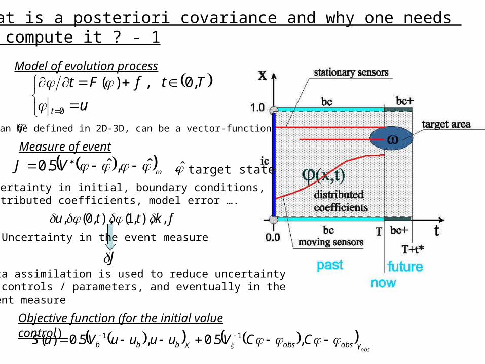
What is a posteriori covariance and why one needs to compute it ? - 1
u
TtfFt
t 0
,0,)(
obsYobsobsXbbb CCVuuuuVuS ,5.0,5.0)( 11
Model of evolution process
Objective function (for the initial value control)
Uncertainty in initial, boundary conditions,distributed coefficients, model error ….
Uncertainty in the event measure
ˆ,ˆ5.0 VJ ̂ - target state
Measure of event
fkttu ,),,1(),,0(,
JData assimilation is used to reduce uncertaintyin controls / parameters, and eventually in the event measure
can be defined in 2D-3D, can be a vector-function

What is a posteriori covariance and why one needs to compute it ? – 2(idea of adjoint sensitivities)
uu
JJ
Trivial relationship between (small) uncertainties in controls / parameters and in the event measure
How to compute the gradient?
1. Direct method ( ) : for solve forward model with compute nRu ni ,...,1 1iu iJ2. Adjoint method:
JfFtL X ,form the Lagrangian
ˆ,, * VFtL X
ˆ,ˆ5.0 VJ
JL
zero
take variation
integrate by parts
X
T VFtuLJ ˆ~,~, 0
If = zero and 0
Tt
0
tu
J
For initial value problem
),(
Gu
J
Generally
Gateaux derivative

What is a posteriori covariance and why one needs to compute it ? - 3
uu
JJ
ssu
JVV
u
J
u
JV
u
J
u
JuuE
u
JJJE uuu
*2/12/1
***,,
scalar
nu
J
u
J
u
J
u
J,...,,
21
- n-vector
sensitivity vector
obsYobsobsXbbb CCVuuuuVuS ,5.0,5.0)( 11
Objective function
bV - the covariance matrix of the background error or a priori covariance (measure of uncertainty in before DA)
Discussion is mainly focused on the question: does the linearised error evolution model (adjoint sensitivity) approximate the non-linear model well? However, another issue is equally (if not more) important:do and how well we really now ?uV
uV -must be a posteriori covariance of the estimation error(measure of uncertainty in after DA)
u
u
How to compute a-posteriori covariance?
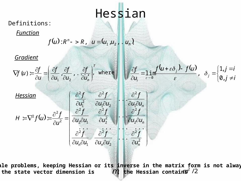
HessianDefinitions:
nn uuuuRRuf ,...,,,: 21
GradientT
nu
f
u
f
u
f
u
fuf
,...,,:)(21
ij
ijufuf
u
fj
j
i ,0
,1,lim
0
, where
Hessian
2
2
2
2
1
2
2
2
22
2
12
21
2
21
2
21
2
2
22
...
............
...
...
::
nnn
n
n
u
f
uu
f
uu
f
uu
f
u
f
uu
fuu
f
uu
f
u
f
u
fufH
Function
For large-scale problems, keeping Hessian or its inverse in the matrix form is not always feasible. If the state vector dimension is , the Hessian contains elements. m 2/2m
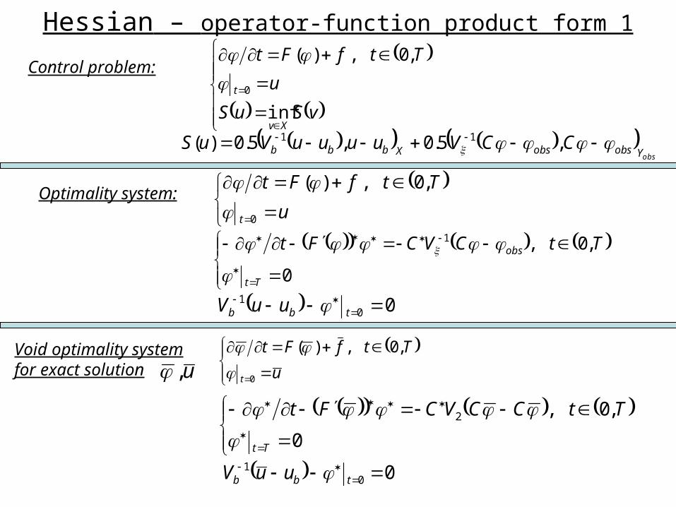
Hessian – operator-function product form 1
vSuS
u
TtfFt
Xv
t
inf
,0,)(
0
obsYobsobsXbbb CCVuuuuVuS ,5.0,5.0)( 11
Control problem:
Optimality system:
u
TtfFt
t 0
,0,)(
0
,0,1
Tt
obs TtCVCFt
001
tbb uuV
Void optimality systemfor exact solution u,
u
TtfFt
t 0
,0,)(
0
,0,2
Tt
TtCCVCFt
001
tbb uuV

Hessian – operator-function product form - 2
u
TtFt
t
0
3 ,0,)~(
Non-linear optimality system for errors:
0
,0,21
Tt
TtCVCFt
0011
tb uV
obsb Cuuuuu 21 ,,,Definition of errors:
,1,0,~
There exists a unique representationIn the form of non-linear operator equation, we call - the Hessian operator.
2211 RRuH
v
TtFt
t 0
,0,0)~(
0
,0,1
Tt
TtCVCFt
01,
tb vVvH
H
Hessian operator-functionproduct definition:
All operators are defined similarly.
,~iR
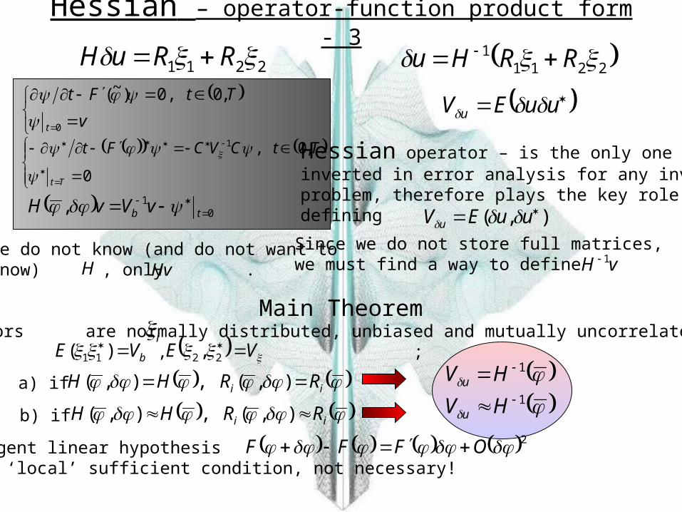
Hessian – operator-function product form - 3
2211 RRuH
v
TtFt
t 0
,0,0)~(
0
,0,1
Tt
TtCVCFt
01,
tb vVvH
We do not know (and do not want to know) , only .H Hv
22111 RRHu
Hessian operator – is the only one to beinverted in error analysis for any inverseproblem, therefore plays the key role indefining !
Since we do not store full matrices, we must find a way to define . vH 1
),( uuEV u
Main TheoremAssume errors are normally distributed, unbiased and mutually uncorrelated, and , ;
ii RRHH ),(,),(
ibVE )( 11 VE
22 ,
a) if 1HV u
b) if ii RRHH ),(,),( 1HV u
(tangent linear hypothesisis a ‘local’ sufficient condition, not necessary!
2 OFFF
uuEV u

Optimal solution error covariance reminder
uV
Holds for any control or combination of controls!

Optimal solution error covariance
Case I: 1) Errors are normally distributed,
ii RRHH ),(,),(2) is moderately non-linear or are small, i.e.)(uF
ii
vH 1
1HV u
Case II:1) errors have arbitrary pdf,
2) ‘weak’ non-linear conditions hold
a) pre-compute (define) .
b) produce single errors implementationusing certain pdf generators. c) compute (no inversion involved)!
Mkuk ,1, ku
d) generate ensemble of
i
Case III:1) Errors have arbitrary pdf,
ku)(1 H
i2) is strongly non-linear (chaotic?) or/and are very big
All as above, but compute by iterative procedure using as a pre-conditioner
i uF
22111 RRHu
e) consider pdf of , which is not normal! f) use it, if you can.
u
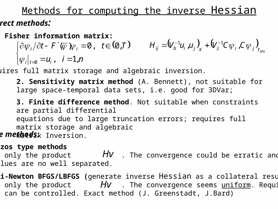
Methods for computing the inverse Hessian
niu
TtFt
iti
ii
,1,
,0,0)(
0
obsYjiXjibij CCVuuVH ,, 11
Direct methods:
1. Fisher information matrix:
Requires full matrix storage and algebraic inversion.
2. Sensitivity matrix method (A. Bennett), not suitable for large space-temporal data sets, i.e. good for 3DVar;
3. Finite difference method. Not suitable when constraints are partial differentialequations due to large truncation errors; requires full matrix storage and algebraicmatrix Inversion.
Iterative methods:
4. Lanczos type methodsRequire only the product . The convergence could be erratic and slow if eigenvalues are no well separated.
5. Quasi-Newton BFGS/LBFGS (generate inverse Hessian as a collateral result)Require only the product . The convergence seems uniform. Requiredstorage can be controlled. Exact method (J. Greenstadt, J.Bard)
Hv
Hv
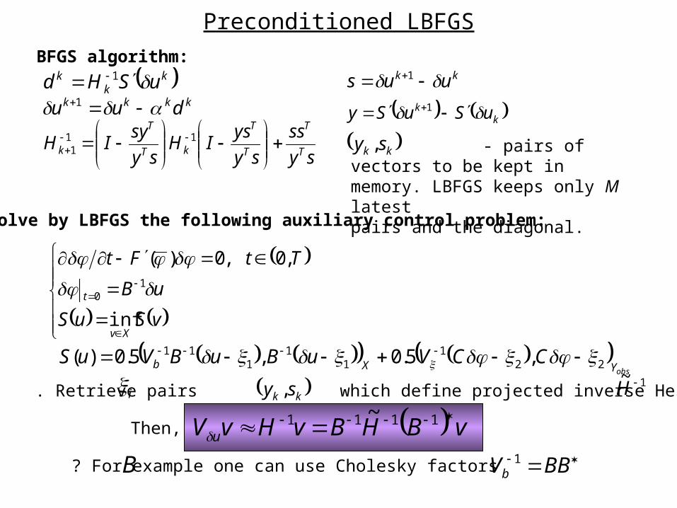
Preconditioned LBFGS
vSuS
uB
TtFt
Xv
t
inf
,0,0)(1
0
Solve by LBFGS the following auxiliary control problem:
BFGS algorithm:
kkk uSHd 1
kkkk duu 1
sy
ss
sy
ysIH
sy
syIH
T
T
T
T
kT
T
k
11
1
kk uus 1
kk uSuSy 1
kk sy , - pairs of vectors to be kept inmemory. LBFGS keeps only M latestpairs and the diagonal.
obsYXb CCVuBuBVuS 22
11
11
11 ,5.0,5.0)(
for chosen . Retrieve pairs which define projected inverse Hessian .i
vBHBvHvV u
1111 ~
1~ H kk sy ,
Then,
How to get ? For example one can use Cholesky factors . BBVb1B

Stupid, yet 100% non-linear ensemble method 1. Consider function as the exact solution to the problem
u
TtfFt
t 0
,0,)(
obsYobsobs
Xbbb
CCV
uuuuVuS
,5.0
,5.0)( 1
2. Assume that and .uub Cobs 3. The solution of the control problem
vSuS
u
TtfFt
Xv
t
inf
,0,)(
0
is
uuu kk 21, Cuu obsbi
.0, uSuu4. Start ensemble loop k=1,…,m.Generate , which correspond to the given pdf. Put Solve the non-linear optimization problem defined in 3).Compute .
5. End ensemble loop.6. Compute statistic
m
k
Tkk uu
mV
1
1ˆ
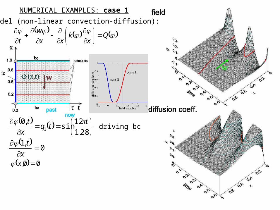
NUMERICAL EXAMPLES: case 1
Q
xk
xx
w
t
Model (non-linear convection-diffusion):
28.1
12sin
,01
ttq
x
t
00, x
- driving bc
0
,1
x
t
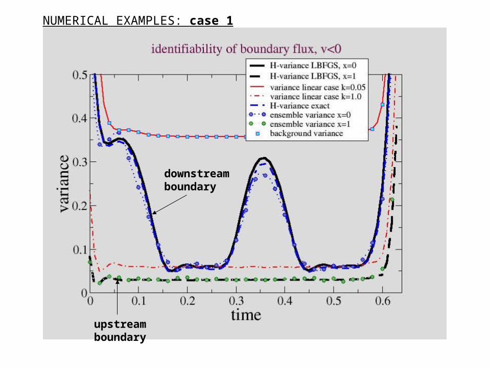
NUMERICAL EXAMPLES: case 1
upstreamboundary
downstreamboundary
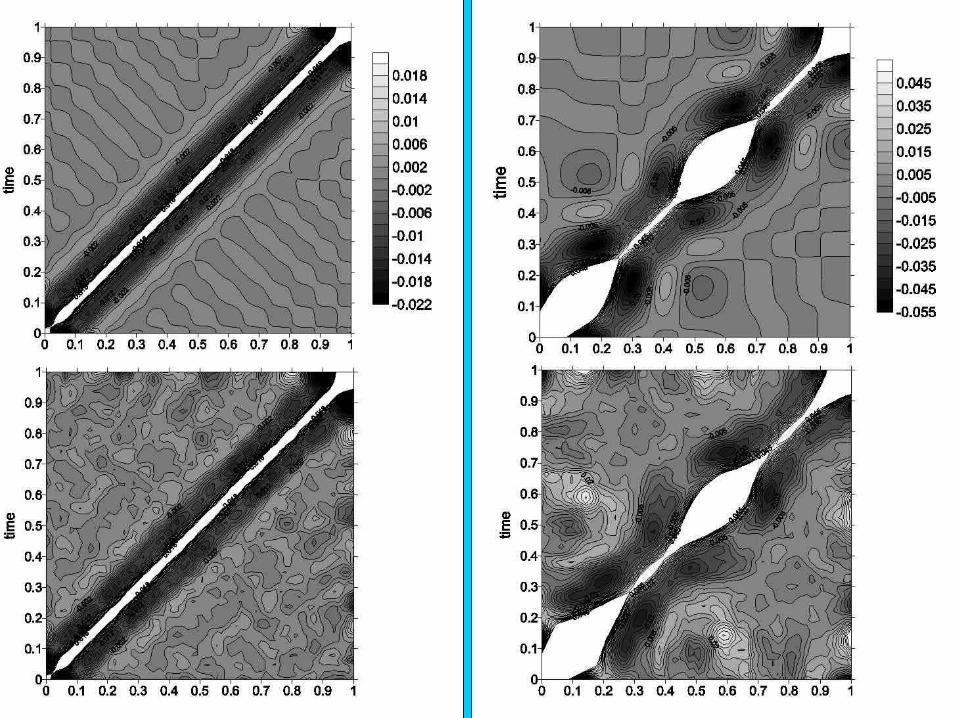

NUMERICAL EXAMPLES: case 2

NUMERICAL EXAMPLES: case 2

NUMERICAL EXAMPLES: case 2
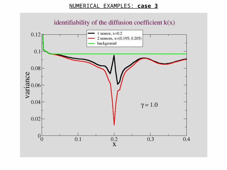
NUMERICAL EXAMPLES: case 3
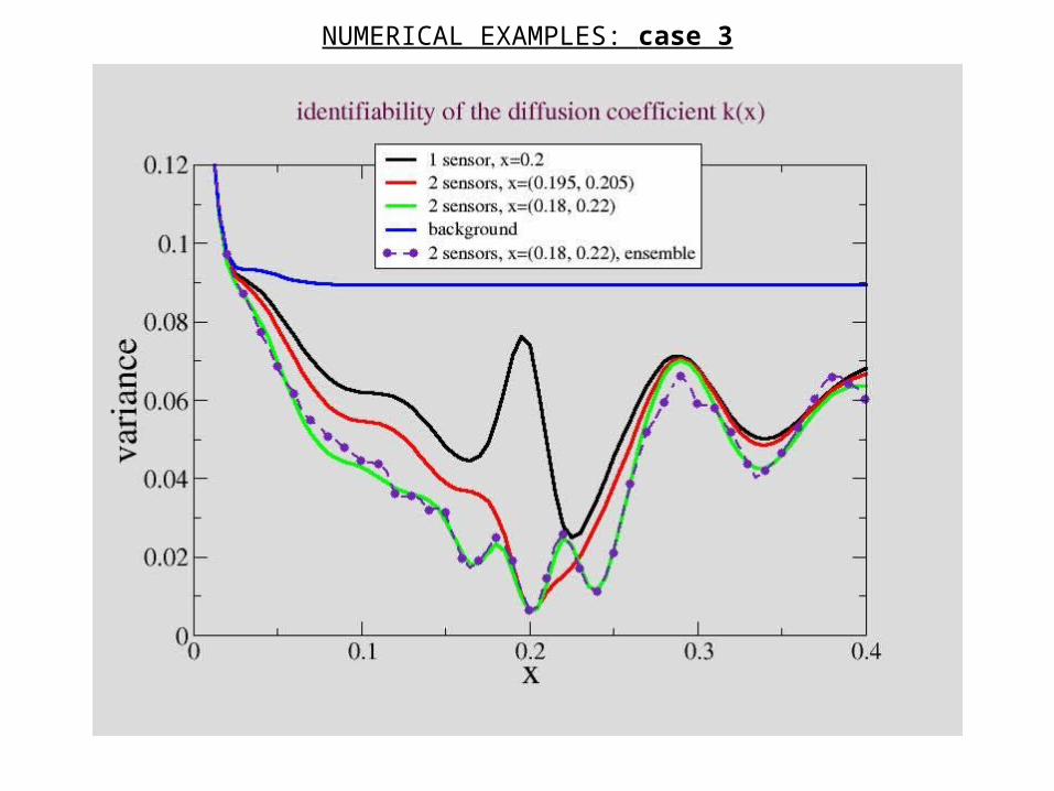
NUMERICAL EXAMPLES: case 3

NUMERICAL EXAMPLES: case 3

SUMMARY1. Hessian plays the crucial role in the analysis of the inverse problem solution errors as the only invertible operator;
2. If errors are normally distributed and constraints are linear the inverse Hessian is itself the covariance operator (matrix) of the optimal solution error;
3. If the problem is moderately non-linear, the inverse Hessian could be a goodapproximation of the optimal solution error covariance far beyond the validity ofthe tangent linear hypothesis. Higher order terms could be considered in problemcanonical decomposition.
4. Inverse Hessian can be well approximated by a sequence of quasi-Newton updates (LBFGS) using the operator-vector product only. This sequence seemsto converge uniformly;
5. Preconditioning dramatically accelerates the computing;
6. The computational cost of computing inverse Hessian should not exceed thecost of data assimilation procedure itself.
7. Inverse Hessian is useful for uncertainty analysis, experiment design, adaptivemeasuring techniques, etc.
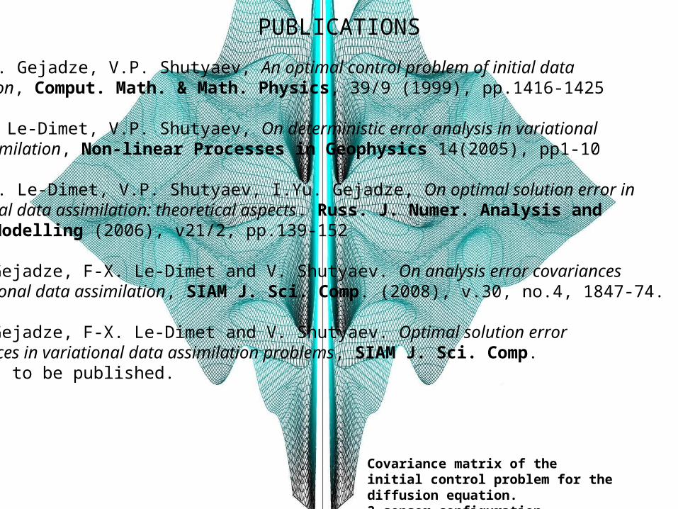
PUBLICATIONS
1. I.Yu. Gejadze, V.P. Shutyaev, An optimal control problem of initial data restoration, Comput. Math. & Math. Physics, 39/9 (1999), pp.1416-1425
2. F-X. Le-Dimet, V.P. Shutyaev, On deterministic error analysis in variationaldata assimilation, Non-linear Processes in Geophysics 14(2005), pp1-10
3. F.-X. Le-Dimet, V.P. Shutyaev, I.Yu. Gejadze, On optimal solution error invariational data assimilation: theoretical aspects. Russ. J. Numer. Analysis andMath. Modelling (2006), v21/2, pp.139-152
4. I. Gejadze, F-X. Le-Dimet and V. Shutyaev. On analysis error covariancesin variational data assimilation, SIAM J. Sci. Comp. (2008), v.30, no.4, 1847-74.
5. I. Gejadze, F-X. Le-Dimet and V. Shutyaev. Optimal solution error covariances in variational data assimilation problems, SIAM J. Sci. Comp. (2008), to be published.
Covariance matrix of the initial control problem for the diffusion equation. 3-sensor configuration