Computing Knopfmacher’s limit, or: My first foray into computational mathematics, reprise

Daniel Lichtblaudanl@wolfram.comWolfram Research, Inc.100 Trade Center Dr.Champaign IL 61820

ACA 2009Montreal, CanadaSession: Applications of Math Software to Mathematical Research

1

ABSTRACT

I will discuss a problem I encountered over a decade ago, and worked on via internet with someone I (alas) never met. It involves a mix of number theory, real analysis, hard−core computation, and some slightly perplexing results.

In brief, we begin with a function expressed as a certain infinite product; Arnold Knopfmacher encountered it in an attempt to approximate the number of irreducible factors of univariate polynomials over Galois fields and raised the question of how to obtain a certain limit to this function. We derive and execute an effective algorithm for the task at hand. We’ll also indicate why the most "obvious" approach does not work well in practice, or at all in theory.

¢ | £

2

The problemAs posed by Arnold Knopfmacher to the Usenet group comp.soft−sys.math.mathematica in January 1999

Let dHkL denote the smallest prime factor of k.

Define m HkL = k - k � dHkLDefine

pHxL = Ûk=2¥ J1- xmHkL

k+1 N1-x

We wish to compute numerically, to at least eight decimal places, the following limit.

limx®1- pHxLThat is to say, we compute the limit as x approaches 1 from the left (lesser) side.

¢ | £

3

Why do we care?

èThere are similar formulas in a paper from 1995 by Knopfmacher and Warlimont, analyzing probabilities related to numbers of irreducible factors of distinct degrees in univariate polynomials over Galois fields

è It’s an interesting computation

¢ | £

4

My history with this problem

I worked on it off and on for several days. Then someone else reading the forum contributed a similar result, but much more precise. His name was Jürgen Tischer, a math department faculty member of Universidad del Valle, Columbia. We corresponded a bit over a period of months, and I wrote up the results. I lost contact with him a year or two later. I had wanted to invite him to this conference. After getting nowhere with an internet search for a current contact address, I learned he had passed away in January of 2008. I felt it fitting to talk a bit about this problem, since it used ideas of his and also was one of my first forays into computational mathematics.

¢ | £

5

Candidate results

There were four responses, with two (mine and Tischer’s) giving roughly the same results. The proposed values were

è 1.3397

è 2 (exactly)

è 2.292

So which is correct?

More important: How do we even know the limit exists?

¢ | £

6

Easy to show...

èA lim sup and lim inf both are readily computed.

èA lim inf is given by ãΓ(the exponential of the Euler gamma constant). This is around 1.871, so...1.3397 will exit stage left.

¢ | £

7

Definitions in Mathematica

d@k_D := Divisors@kD@@2DDm@k_D := k - k

d@kD

p@x_D :=Ûk=2¥ J1 - xm@kD

k+1N

1 - x

General idea: Start with

Ûk=2¥ 1- x

c k2s

k+1

1-x < p@xD < Ûk=2¥ J1- xk-1

k+1 N1-x

Now take logs to get summations. Expand logs at 1 as power series, obtaining double summations. Switch order of summation (requires justification), and we find that log of a lim sup is Γ + log H2L. Finding a lim inf is similar though a bit more work.

¢ | £

8

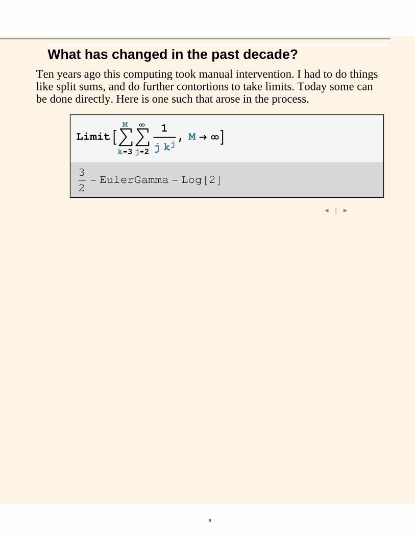
What has changed in the past decade?Ten years ago this computing took manual intervention. I had to do things like split sums, and do further contortions to take limits. Today some can be done directly. Here is one such that arose in the process.

LimitAâk=3

M

âj=2

¥ 1

j kj, M ® ¥E

3

2- EulerGamma - Log@2D

¢ | £

9

A start at approximating the actual limit

èTruncate the series for the logarithm

èEvaluate using exact or high precision arithmetic at x = 1

èExponentiate

Log@p@xDD = -Log@1- xD +â2 k

LogB1- xk�2k + 1

F +

â2Ik,3 k

LogB1- x2 k�3k + 1

F + ...=

-âk=1

¥xk

k+â

2 k

xk�2k + 1

+â2 k

âj=2

¥x j k�2

j Hk + 1L j +

â2Ik,3 k

x2 k�3k + 1

+ â2Ik,3 k

âj=2

¥xH2�3L j k

j Hk + 1L j + ...

(The series that get truncated are the summations inj). From this tactic I was able to get 2.292 (so, as you may have guessed, exact 2 was not the correct result either).

j ¢ | £

10

Troublesome aspects

There are serious problems with this approach.

èDifficult to get good precision

è (Related, but more serious) It is quite difficult to bound the error. Indeed, it is not easy to show we have convergence.

¢ | £

11

Tischer’s idea

Figure out exact forms for some of the infinite sums, so as to avoid truncation. In parts we cannot compute exactly, show that error is much better than what we have from above approach.

Start by writing log Hp HxLL (after a bit of algebra) as

x +x2

2+âk=2

¥xk+1

k + 1-xm@kDk + 1

-

âk=2

¥

âj=2

¥ K1jO xm@kD

k + 1

j

Proposition: This approaches Γ + logH2L+Úk=2¥ J xk+1

k+1-

xmHkLk+1N as x® 1 from

below.

¢ | £

12

Sketch of proof

Clearly we only need focus on the double summation. Switch summation order and use

âk=2

¥xk

k + 1

j

£âk=2

¥xm@kDk + 1

j

£âk=2

¥xk�2

k + 1

j

Middle is squeezed to

âk=2

¥

K 1

k + 1O

j

So we can find:

âj=2

¥ 1

jâk=2

¥

K 1

k + 1Oj

1

2H3 - 2 EulerGamma - 2 Log@2DL

Several steps require justification! We interchanged a summation order, then a sum with a limit...

¢ | £

13

That remaining summation

We now need to estimate the remaining part. We split by smallest divisors.

âk=2

¥xk+1

k + 1-

xm@kDk + 1

=

âd@kD=2

¥xk+1

k + 1-

xI k2 Mk + 1

+ âd@kD=3

¥xk+1

k + 1-

xI2 k3 M

k + 1+

âd@kD=5

¥xk+1

k + 1-

xI4 k5 M

k + 1+ ...

The reordering is fine: for 0< x < 1 each term is negative so we can do this.

Now we need to compute

âd@kD=Prime@ jD

¥xk+1

k + 1-

xJHPrime@ jD-1L k

Prime@ jD N

k + 1

¢ | £

14

Remaining summation...

We need some functions.

q@j_D :=äk=1

j

Prime@kD

r@j_D :=äk=1

j-1

HPrime@kD - 1L

frac@j_D := r@jDq@jD

The terms k for which primeH jL is the smallest divisor larger than 1 fall into finitely many congruence sets. For example, when the prime in question is 5, the applicable values for k are 85, 25, 35, 55, 65, 85, 95, ...<. This may be partitioned as 85, 35, 65, 95, ...< and 825, 55, 85, ...<. In each case, the step size is 30.

¢ | £

15

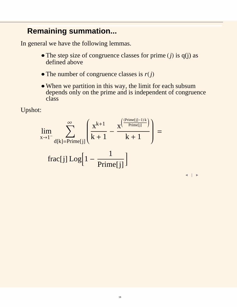
Remaining summation...

In general we have the following lemmas.

èThe step size of congruence classes for primeH jL is q(j) as defined above

èThe number of congruence classes is rH jLèWhen we partition in this way, the limit for each subsum

depends only on the prime and is independent of congruence class

Upshot:

limx®1-

âd@kD=Prime@ jD

¥xk+1

k + 1-

xJHPrime@ jD-1L k

Prime@ jD N

k + 1=

frac@ jD LogB1- 1

Prime@ jD F¢ | £

16

Remaining summation...

limx®1-âk=2

¥xk+1

k + 1-

xm@kDk + 1

=

âj=1

M

frac@ jD LogB1- 1

Prime@ jD F +

limx®1-

âd@kD³Prime@M+1D

¥xk+1

k + 1-

xIHd@kD-1L k

d@kD Mk + 1

We can readily bound that tail sum.

tailsumbnd = SumA xk+1

k + 1-

xHPrime@MD-1L k

Prime@MD

k + 1, 8k, 0, ¥<E

-1

xJx Log@1 - xD -x

1Prime@MD LogAx- 1

Prime@MD J-x + x 1Prime@MDNEN

Limit@tailsumbnd, x ® 1, Direction ® 1DLogA1 - 1

Prime@MDE¢ | £

17

Computing our estimate

We can now put all this together.

estimate@n_D :=âj=1

n

frac@jD LogA1 - 1

Prime@jDE

error@n_D := âj=n+1

¥

frac@jD LogA1 - 1

Prime@jDE

numestimate@n_, prec_D :=ModuleA8sum = -1�2*Log@2D, frac = 1�2,

p1 = Prime@1D, p2<,DoAp2 = N@Prime@jD, precD;frac *=

p1 - 1

p2;

sum += frac*LogA1 - 1

p2E;

p1 = p2,8j, 2, n<E;8frac*p2, sum<E

Timing@8mfact, est< =numestimate@2*10^8+ 1, 25DD

817524.4, 80.025332454849260739,-0.4408622662133543648819837<<

¢ | £

18

Computing...

Upper bound on error. Set n = 2´ 10^8.

mfact âj=n+1

¥1

Prime@ jD LogB1- 1

Prime@ jD F <

mfactK1+ 1

Prime@nD O âj=n+1

¥1

j2 Log@ jD2 <

57�2000àn

¥ 1

Hj log@jDL2 âjerrormax =H57�2000L Integrate@1�Hj Log@jDL^2,8j, 2*10^8, Infinity<D

N@errormaxD1

200057 KExpIntegralEi@-Log@200000 000DD +

1

200 000 000 Log@200 000 000DO

3.54571´10-13

¢ | £

19

Computing... Finally we get our estimate and error bound.

p1 = Exp@EulerGamma + Log@2D + estD2.292173695248049690410395

errbound = N@Exp@errormaxD - 1D*p18.12817´10-13

¢ | £

20

Further items of interest

We can investigate the error term of the "naive" summation approach by looking at the series of the log of the product.

logp@x_, n_D := NormalA

SeriesA-Log@1 - xD +âk=2

2*n

LogA1 - xm@kD

k + 1E,

8x, 0, n<EEWe can use this to get the signs of the terms. I show them in a run−length form.

880, 1<, 81, 1<, 8-1, 1<, 81, 1<, 8-1, 1<, 81, 1<, 8-1, 1<, 81, 3<,8-1, 1<, 81, 1<, 8-1, 1<, 81, 1<, 8-1, 1<, 81, 1<, 8-1, 1<,81, 1<, 8-1, 1<, 81, 1<, 8-1, 1<, 81, 1<, 8-1, 1<, 81, 3<,8-1, 1<, 81, 1<, 8-1, 1<, 81, 1<, 8-1, 1<, 81, 3<, 8-1, 1<,81, 1<, 8-1, 1<, 81, 1<, 8-1, 1<, 81, 1<, 8-1, 1<, 81, 1<,8-1, 1<, 81, 1<, 8-1, 1<, 81, 1<, 8-1, 1<, 81, 3<, 8-1, 1<,81, 1<, 8-1, 1<, 81, 1<, 8-1, 1<, 81, 3<, 8-1, 1<, 81, 1<,8-1, 1<, 81, 1<, 8-1, 1<, 81, 3<, 8-1, 1<, 81, 1<, 8-1, 1<,81, 1<, 8-1, 1<, 81, 1<, 8-1, 1<, 81, 1<, 8-1, 1<, 81, 1<,8-1, 1<, 81, 1<, 8-1, 1<, 81, 3<, 8-1, 1<, 81, 3<, 8-1, 1<,81, 1<, 8-1, 1<, 81, 1<, 8-1, 1<, 81, 1<, 8-1, 1<, 81, 1<,8-1, 1<, 81, 1<, 8-1, 1<, 81, 1<, 8-1, 1<, 81, 1<, 8-1, 1<<

They seem to alternate, with sporadic runs of three positive terms. Strange...

¢ | £

21

Further items...

But stranger is the magnitudes of these coefficients. They are not even

bounded by OI 1nM.

Can show:

èThey are bounded by OI log @log@ nDDn

MèThis bound is tight (we can show that infinitely many

coefficients will approach it closely).

èThe ones that approach closely have interesting factorization patterns (which is why they approach closely).

èFiguring this out was more math than computation (our jobs are not going to the machines just yet).

Upshot: a naive summation will clearly give very poor convergence.

¢ | £

22

Some open problems

èUnderstand the sign patterns of error approximants.

èFind a more efficient way to compute the estimate to high precision.

èFind an exact closed form for the limit.

èAutomate more of the symbolic analysis: some still requires manual intervention.

èDetermine whether the error bound/estimate is tight. If not, improve it (this would be a "cheap" way of getting more digits).

¢ | £

23

ReferencesA. Knopfmacher (1999a). Usenet news group post to comp.soft−sys.math.mathematica.http://library.wolfram.com/mathgroup/archive/1999/Jan/msg00023.html

A. Knopfmacher and R. Warlimont (1995). Distinct degree factorizations for polynomials over a finite field. Transactions of the American Mathematical Society 347(6):2235−2243.

DL (1999). The evaluation of Knopfmacher’s curious limit. Manuscript.

J. Tischer (1999). Usenet news group post to comp.soft−sys.math.mathematica.http://library.wolfram.com/mathgroup/archive/1999/Jan/msg00355.html

¢ | £

24