computing the sparse matrix vector product using block ... the sparse matrix vector product using...
TRANSCRIPT
Submitted 12 January 2018Accepted 2 April 2018Published 30 April 2018
Corresponding authorBérenger Bramas,[email protected]
Academic editorNick Higham
Additional Information andDeclarations can be found onpage 21
DOI 10.7717/peerj-cs.151
Copyright2018 Bramas and Kus
Distributed underCreative Commons CC-BY 4.0
OPEN ACCESS
Computing the sparse matrix vectorproduct using block-based kernelswithout zero padding on processors withAVX-512 instructionsBérenger Bramas and Pavel KusApplication Group, Max Planck Computing and Data Facility, Garching, Allemagne
ABSTRACTThe sparsematrix-vector product (SpMV) is a fundamental operation inmany scientificapplications from various fields. TheHigh Performance Computing (HPC) communityhas therefore continuously invested a lot of effort to provide an efficient SpMV kernelon modern CPU architectures. Although it has been shown that block-based kernelshelp to achieve high performance, they are difficult to use in practice because of thezero padding they require. In the current paper, we propose new kernels using theAVX-512 instruction set, which makes it possible to use a blocking scheme withoutany zero padding in the matrix memory storage. We describe mask-based sparsematrix formats and their corresponding SpMV kernels highly optimized in assemblylanguage. Considering that the optimal blocking size depends on the matrix, we alsoprovide a method to predict the best kernel to be used utilizing a simple interpolationof results from previous executions. We compare the performance of our approachto that of the Intel MKL CSR kernel and the CSR5 open-source package on a set ofstandard benchmark matrices. We show that we can achieve significant improvementsin many cases, both for sequential and for parallel executions. Finally, we provide thecorresponding code in an open source library, called SPC5.
Subjects Distributed and Parallel Computing, Scientific Computing and SimulationKeywords SpMV, Code Optimization, SIMD, Vectorization, HPC
INTRODUCTIONThe sparse matrix-vector product (SpMV) is an important operation in many applications,which often needs to be performed multiple times in the course of the algorithm. It is oftenthe case that no matter how sophisticated the particular algorithm is, most of the CPU timeis spent in matrix-vector product evaluations. The prominent examples are iterative solversbased on Krylov subspaces, such as the popular CG method. Here the solution vector isfound after multiple matrix-vector multiplications with the same matrix. Since in manyscientific applications a large part of the CPU time is spent in the solution of the resultinglinear system and the matrix is stored in a sparse manner, improving the efficiency of theSpMV on modern hardware could potentially leverage the performance of a wide range ofcodes.
How to cite this article Bramas and Kus (2018), Computing the sparse matrix vector product using block-based kernels without zeropadding on processors with AVX-512 instructions. PeerJ Comput. Sci. 4:e151; DOI 10.7717/peerj-cs.151
One of the possible approaches towards the improvement of the SpMV is to takeadvantage of a specific sparsity pattern. For example, the diagonal storage (DIA) (Saad,1994) or jagged diagonal storage (JAD) (Saad, 2003) are designed for matrices that aremostly diagonal or band-diagonal. However, unless ensured by the matrix producingmethod design, it is not straightforward to evaluate in advance when a given matrix’sstructure is well suited for a specific format. This has been the main motivation to providegeneral SpMV like block-based schemes, as described in (Vuduc, 2003; Im, Yelick & Vuduc,2004;Vuduc & Moon, 2005;Vuduc, Demmel & Yelick, 2005; Im & Yelick, 2001). These typesof kernels make it possible to use the SIMD/vectorization capability of the CPU, but theyalso are required to fill the blocks with zeros to avoid a transformation of the loaded valuesfrom the memory before computation. The extra memory usage and the ensuing transfersdrastically reduce the effective performance. Moreover, it has been shown that there is noideal block size that works well for all matrices.
In the current study, we attempt to address the mentioned issues, namely problemscaused by zero padding and optimal block selection. The recent AVX-512 instructionset provides the possibility to load fewer values than a vector can contain and to expandthem inside the vector (dispatching them in order). This feature allows for fully vectorizedblock-based kernels without any zero padding in the matrix storage. Additionally, weprovide a method to select the block size that is most likely to provide the best performanceanalyzing the execution times of the previous runs.
The contributions of the study are the following:
• we study block based SpMV without padding with AVX-512,• we describe an efficient implementation targeting the next generation of Intel’s HPCarchitecture,• we provide a record-based strategy to choose the most appropriate kernel (usingpolynomial interpolation in sequential, and linear regression for shared-memory parallelapproaches),• the paper introduces the SPC5 package that includes the source code related to thepresent study (https://gitlab.mpcdf.mpg.de/bbramas/spc5).
The rest of the paper is organized as follows: ‘Background’ gives background informationrelated to vectorization and SpMV. We then describe our method in ‘Design of Block-based SpMV without Padding’ and show its performance on selected matrices of variousproperties in ‘Performance Analysis’. Comparison of various variants of our method usingdifferent blocking is provided. In ‘Performance Prediction and Optimal Kernel Selection’we propose a systematic approach towards the selection of an optimal kernel based on easilyobtained properties of the given matrix. Finally, we draw conclusions in ‘Conclusions’.
BACKGROUNDIn this section we recall a few rather well known facts regarding the vectorization inmodernprocessor architectures and about existing sparse matrix vector product implementations.
Bramas and Kus (2018), PeerJ Comput. Sci., DOI 10.7717/peerj-cs.151 2/23

VectorizationThe growth of computing power with new generations of processors has been advancing fordecades. One of its manifestations, which is of particular interest for scientific computing, isthe steady growth of peak performance in terms of the number of floating point operationsper second. What has changed recently, however, is the way the hardware manufacturerssustain this growth. With the effective halt in the growth of processor frequencies, most ofthe increase of computing power is achieved through increasing the number of cores andthe ability of each individual core to perform each operation on a vector of certain lengthusing one instruction only. This capability is named vectorization or single instruction onmultiple data (SIMD).
The AVX-512 (Intel, 2016) is an extension to the x86 instruction set dedicated tovectorization. It supports a 512 bits vector length, which corresponds to 16 single precisionor eight double precision floating point values, and we use the term VEC_SIZE to refer tothe number of values inside a vector. This instruction set provides new operations such asload/store operations tomove data between themainmemory and the CPU’s registers. Oneof these new instructions is the vexpandpd(mask,ptr), where mask is an unsigned integerof VEC_SIZE bits and ptr a pointer to an array of single or double precision floating pointvalues. This instruction loads one value for each bit that is set to one in the mask, andmove them to the corresponding position in the output vector. For example, in doubleprecision, vexpandpd(10001011b,ptr) returns a vector equal to [ptr[0], ptr[1], 0, ptr[2], 0,0, 0, ptr[3]], where ptr[i] refers to the values at position i in the array of address ptr, andconsidering that the mask is written from right to left. One can see this instruction as ascatter from the main memory to the vector.
Sparse Matrix Vector Product (SpMV)If there is any advantage of exploiting the zeros, for example, by saving time or memory,then the matrix should be considered as sparse (Wilkinson et al., 1971). However, removingthe zeros from the matrix leads to new storage and new computational kernels. While thegain of using a sparse matrix instead of a dense one can be huge in terms of memoryoccupancy and speed, the effective Flop rate of a sparse kernel generally remains lowcompared to its dense counterpart. In fact, in a sparse matrix storage, we provide a wayto know the respective column and row of each non-zero value (NNZ). Therefore, thegeneral SpMV is a bandwidth/memory bound operation because it pays the price ofthis extra storage and leads to a low ratio of Flop to perform against data occupancy.Moreover, the sparsity structure of the matrix makes it difficult to have data reuse or to usevectorization.
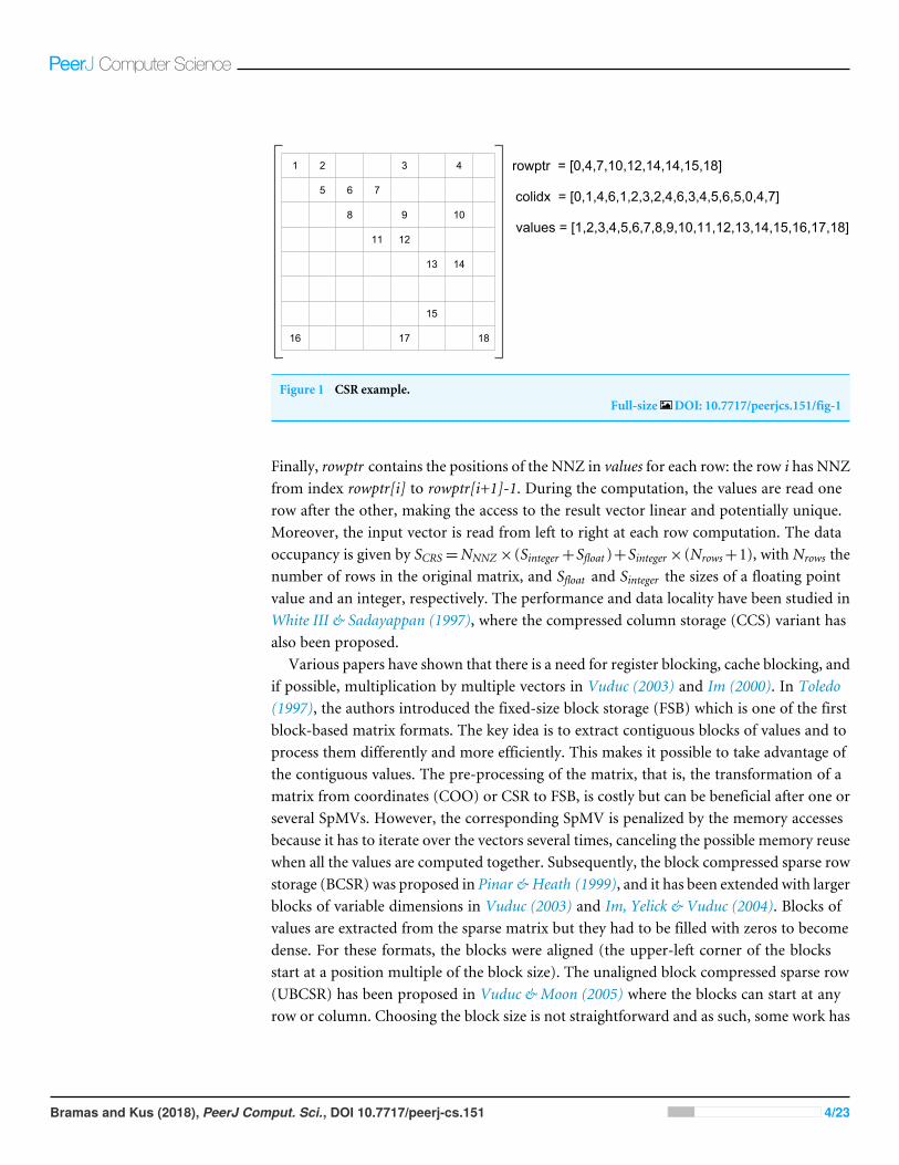
The compressed row storage (CRS), also known as the compress sparse row (CSR)storage (Barrett et al., 1994), is a well-known storage and is used as a de-facto standardin SpMV studies. Its main idea is to avoid storing individual row indexes for each NNZvalue. Instead, it counts the number of values that each row contains. Figure 1 presentsan example of the CRS storage. The NNZ values of the original matrix are stored in avalues array in row major (one row after the other) and in column ascending order. In asecondary array colidx we store the column indexes of the NNZ values in the same order.
Bramas and Kus (2018), PeerJ Comput. Sci., DOI 10.7717/peerj-cs.151 3/23
1 2 3 4
5 6 7
8 9 10
11 12
13 14
15
16 17 18
values = [1,2,3,4,5,6,7,8,9,10,11,12,13,14,15,16,17,18]
colidx = [0,1,4,6,1,2,3,2,4,6,3,4,5,6,5,0,4,7]
rowptr = [0,4,7,10,12,14,14,15,18]
Figure 1 CSR example.Full-size DOI: 10.7717/peerjcs.151/fig-1
Finally, rowptr contains the positions of the NNZ in values for each row: the row i has NNZfrom index rowptr[i] to rowptr[i+1]-1. During the computation, the values are read onerow after the other, making the access to the result vector linear and potentially unique.Moreover, the input vector is read from left to right at each row computation. The dataoccupancy is given by SCRS=NNNZ×(Sinteger+Sfloat )+Sinteger×(Nrows+1), with Nrows thenumber of rows in the original matrix, and Sfloat and Sinteger the sizes of a floating pointvalue and an integer, respectively. The performance and data locality have been studied inWhite III & Sadayappan (1997), where the compressed column storage (CCS) variant hasalso been proposed.
Various papers have shown that there is a need for register blocking, cache blocking, andif possible, multiplication by multiple vectors in Vuduc (2003) and Im (2000). In Toledo(1997), the authors introduced the fixed-size block storage (FSB) which is one of the firstblock-based matrix formats. The key idea is to extract contiguous blocks of values and toprocess them differently and more efficiently. This makes it possible to take advantage ofthe contiguous values. The pre-processing of the matrix, that is, the transformation of amatrix from coordinates (COO) or CSR to FSB, is costly but can be beneficial after one orseveral SpMVs. However, the corresponding SpMV is penalized by the memory accessesbecause it has to iterate over the vectors several times, canceling the possible memory reusewhen all the values are computed together. Subsequently, the block compressed sparse rowstorage (BCSR) was proposed in Pinar & Heath (1999), and it has been extended with largerblocks of variable dimensions in Vuduc (2003) and Im, Yelick & Vuduc (2004). Blocks ofvalues are extracted from the sparse matrix but they had to be filled with zeros to becomedense. For these formats, the blocks were aligned (the upper-left corner of the blocksstart at a position multiple of the block size). The unaligned block compressed sparse row(UBCSR) has been proposed in Vuduc & Moon (2005) where the blocks can start at anyrow or column. Choosing the block size is not straightforward and as such, some work has
Bramas and Kus (2018), PeerJ Comput. Sci., DOI 10.7717/peerj-cs.151 4/23

been done to provide a mechanism to find it (Vuduc, Demmel & Yelick, 2005; Im & Yelick,2001).
The main drawback of the compressed sparse matrix format is that the data locality isnot preserved and it is thus more difficult to vectorize the operations. A possible attemptto solve this problem is by combining a sparse and dense approach: a certain block size isselected and the matrix is covered by blocks of this size so that all non-zero elements of thematrix belong to some block. The positions of the blocks are then stored in sparse fashion(using row pointers and column indices), while each block is stored as dense, effectively bystoring all elements belonging to the block explicitly, including zeros. This leads to paddingthe non-zero values in the values array by zeros and thus increases memory requirements.The immense padding implied by their design led to the failure to adopt these methods inreal-life calculations.
The authors from Yzelman (2015) show how to use gather/scatter instructions tocompute block-based SpMV. However, the proposed method still fill the blocks with zerosin the matrix storage to ensure that blocks have values of a fixed size. Moreover, they usearrays of integers, needed by the scatter/gather operations, which adds important memoryoccupancy to the resulting storage. The author also describe the bit-based methods as notefficient in general, but we show in the current study that approaches are now efficient.The proposed mechanism from Buluc et al. (2011) is very similar to our work. The authorsdesign a SpMV using bit-masks. However, they focus on symmetric matrices and buildtheir work on top of SSE, which requires several instructions to do what can be done in asingle now. In Kannan (2013), the authors use bitmasks to represent the positions of theNNZ inside the blocks as we do here. However, they use additional integers to represent theposition of the blocks in the matrix, while we partially avoid aligning the block vertically.In addition, they fail to develop a highly-tuned and optimized version of their kernel inorder to remain portable. Consequently, they do not use vectorization explicitly and theirimplementation is not parallel.
More recent work has been done, pushed by the research on GPUs and the availability ofmanycore architectures. In Liu et al. (2013), the authors extend the ELLAPACK format thatbecame popular due to its high performance on GPUs, and adapt it to the Intel KNC. Theyprovide some metrics to estimate if the computation of a matrix is likely to be memoryor computation bounded. They conclude that block-based schemes are not expected tobe efficient because the average number of NNZ per block can be low. As we will show inthe current study, this is only partially true because block-based approaches require lesstransformation of the input matrix and in extreme cases it is possible to use the block maskto avoid useless memory load. The authors of Liu et al. (2013) also propose an auto-tuningmechanism to balance the work between threads, and their approach appears efficient onthe KNC. The authors of Kreutzer et al. (2014) define the SELL-C- σ format as a variant ofSliced ELLPACK. The key idea of their proposal is to provide a single matrix format thatcan be used on all common HPC architectures including regular CPUs, manycore CPUs,and GPUs. We consider that focusing on CPUs only could lead to better specific matrixstorage. In Liu & Vinter (2015) the authors also target CPUs and GPUs and introduce a
Bramas and Kus (2018), PeerJ Comput. Sci., DOI 10.7717/peerj-cs.151 5/23
new matrix format, called CSR5. A corresponding source code is freely available online.We include their code in our performance benchmark.
Matrix permutation/reorderingPermutation of the rows and/or columns of a sparse matrix can improve the memoryaccess pattern and the storage. A well-known technique called Cuthill–McKee from Cuthill& McKee (1969) tries to make a matrix bandwidth by applying a breadth-first algorithmon a graph which represents the matrix structure such that the resulting matrices havegood properties for LU decomposition. However, the aim of this algorithm is not toimprove the SpMV performance even though the generated matrices may have better datalocality.
In Pinar & Heath (1999), a method is proposed to have specifically more contiguousvalues in rows or columns. The idea is to create a graph from a matrix where each columnis a vertex and by connecting all the vertices with weighted edges. The weights come fromdifferent formulations, but they represent the interest of putting two columns contiguously.Then, a permutation is found by solving the traveling salesman problem (TSP) to obtaina path that goes through all the nodes but only once and that minimizes the cost of thetotal weight of the path. Therefore, a path in the graph represents a permutation; when weadd a node to a path, it means that we aggregate a column to a matrix in construction. Themethod has been updated in Vuduc & Moon (2005), Pichel et al. (2005) and Bramas (2016)with different formulas.
The permutation of the matrices has been left aside from the current study but as inmost other approaches, any improvement to the shape of the matrix will certainly improvethe efficiency of our kernels by reducing the number of blocks.
DESIGN OF BLOCK-BASED SpMV WITHOUT PADDINGIn this section, we will elaborate on an alternative approach to the existing block-basedstorage by exploiting the mask features from the AVX-512 instruction set. Instead ofpadding the nonzero values with zeros to fill the whole blocks, we store an array of maskswhere each mask corresponds to one block and describes how many non-zeros there areand on which positions within the block.We also describe the corresponding SpMV kernelsand discuss their optimization and parallelization.
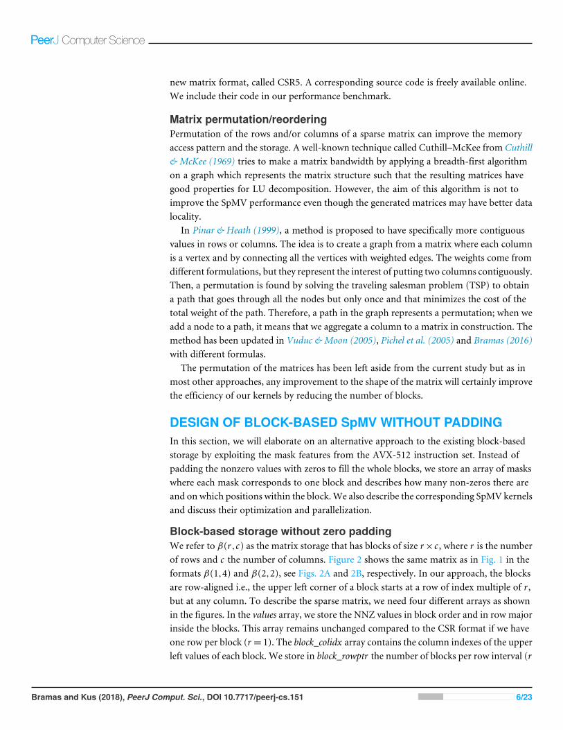
Block-based storage without zero paddingWe refer to β(r,c) as the matrix storage that has blocks of size r×c , where r is the numberof rows and c the number of columns. Figure 2 shows the same matrix as in Fig. 1 in theformats β(1,4) and β(2,2), see Figs. 2A and 2B, respectively. In our approach, the blocksare row-aligned i.e., the upper left corner of a block starts at a row of index multiple of r ,but at any column. To describe the sparse matrix, we need four different arrays as shownin the figures. In the values array, we store the NNZ values in block order and in row majorinside the blocks. This array remains unchanged compared to the CSR format if we haveone row per block (r = 1). The block_colidx array contains the column indexes of the upperleft values of each block. We store in block_rowptr the number of blocks per row interval (r
Bramas and Kus (2018), PeerJ Comput. Sci., DOI 10.7717/peerj-cs.151 6/23

1 2 3 4
5 6 7
8 9 10
11 12
13 14
15
16 17 18
values = [1,2,3,4,5,6,7,8,9,10,11,12,13,14,15,16,17,18]
block_masks = [(0011) (0101) (0111) (0101) (0001) (0011) (0011) (0001) (0001) (0101)]
block_colidx = [0,4,1,2,6,3,5,5,0,4]
block_rowptr = [0,2,3,5,6,7,7,8,10]
nb_blocks = 10 1 2 3 4
5 6 7
8 9 10
11 12
13 14
15
16 17 18
values = [1,2,5,6,7,3,4,8,11,9,12,10,13,14,16,15,17,18]
block_masks = [(1011) (1100) (0001) (0001) (1001) (0101) (0001) (0011) (0100) (0110) (0100)]
block_colidx = [0,2,4,6,2,4,6,5,0,4,7]
block_rowptr = [0,4,7,8,11]
nb_blocks = 11
(A) (B)
Figure 2 SPC5 format examples. The masks are written in conventional order (greater/right, lower/left). (A) SPC5 BCSR Example for β(1,4). Thevalues array is unchanged compared to the CSR storage. (B) SPC5 BCSR Example for β(2,2).
Full-size DOI: 10.7717/peerjcs.151/fig-2
consecutive rows). Finally, the block_masks array provides one mask of r×c bits per blockto describe the sparsity structure inside each block.
We note Nblocks(r,c) the number of blocks of size r× c obtained from a given matrix.The average number of NNZ per block is then Avg (r,c)=NNNZ/Nblocks(r,c). The memoryoccupancy is given by (in bytes) :
O(r,c)=Ovalues(r,c)+Oblock_colidx(r,c)+Oblock_rowptr (r,c)+Oblock_masks(r,c)Ovalues(r,c)=NNNZ ×Sfloat
Oblock_rowptr (r,c)≈Nrows
r×Sinteger
Oblock_colidx(r,c)=Nblocks(r,c)×Sinteger
Oblock_masks(r,c)=Nblocks(r,c)× r× c
8,
(1)
with Sfloat and Sinteger the sizes of a floating point value and an integer, respectively. Afterputting two terms together and substituting for Nblocks(r,c)=NNNZ/Avg (r,c) we get thetotal occupancy
O(r,c)=NNNZ ×Sfloat +Nrows×Sinteger
r+NNNZ ×
8×Sinteger+ r× c8×Avg (r,c)
. (2)
Let us now compare with the memory occupancy of the CSR format, which is
OCSR=NNNZ ×Sfloat +Nrows×Sinteger+NNNZ ×Sinteger . (3)
The first term is the same for both storages. This is thanks to the fact that we do not usezero padding in the values array, as it has been discussed before. The second term is onlyrelevant for the very sparse matrices: otherwise NNNZ �Nrows) is clearly either the same(if r = 1) or smaller for our storage whenever r > 1. The last term is smaller for ourstorage if
Avg (r,c)> 1+r× c
8×Sinteger, (4)
Bramas and Kus (2018), PeerJ Comput. Sci., DOI 10.7717/peerj-cs.151 7/23

which should be usually true unless the blocks are very poorly filled. If we consider theusual size of the integer Sinteger = 4, we need average filling of at least 1+ 1
4 for β(1,8), 1+12
for β(2,8) and β(4,4), and 2 for β(4,8) and β(8,4), respectively.Memory occupancy is an important measure, because the SpMV is usually a memory-
bound operation and therefore, reducing the total amount of memory to perform the samenumber of floating point operations (Flop) is expected to be beneficial by shifting to amore computational-bound kernel. Indeed, using blocks helps to remove the usual SpMVlimits in terms of a poor data reuse of the NNZ values and non-contiguous accesses on thedense vectors.
SpMV kernels for β(r,c) storagesWe provide the SpMV kernel that works for any block size in Algorithm 1. Thecomputation iterates over the rows with a step r since the blocks are r-aligned. Then,it iterates over all the blocks inside a row interval, from left to right, starting fromthe block of index mat.block_rowptr[idxRow/r] and ending before the block of indexmat.block_rowptr[idxRow/r+1] (line 7). The column index for each block is given bymat.block_colidx and stored in idxCol (line 8). To access the values that correspond to ablock, we must use a dedicated variable idxVal, which is incremented by the number ofbits set to 1 in the masks. The scalar algorithm relies on an inner loop of index k to iterateover the bits of the masks. This loop can be vectorized in AVX-512 using the vexpandinstruction such that the arithmetic operations between y, x andmat.values are vectorized.
In Algorithm 1, all the blocks from a matrix are computed similarly regardless whethertheir masks contain all ones or all zeros. This can become unfavorable in the case ofextremely sparse matrices: most of the blocks will then contain a single value and onlyone bit of the mask will be equal to 1. This implies two possible overheads; first we loadthe values from the matrix using the vexpand instruction instead of a scalar move, andsecond, we load a full vector from x and use vector-based arithmetic instruction. This iswhy we propose an alternative approach shown in Algorithm 2 for β(1,VEC_SIZE). Theidea is to use two separate inner loops to proceed differently on the blocks dependingon whether they contain only one value or more than one value. However, having a testinside the inner loop could kill the instruction pipeline and the speculation from the CPU.Instead, we use two separate inner loops and jump from one loop to the other one whenneeded. Indeed, using goto commandmight seem strange, but it is justified by performanceconsiderations and, since the algorithm is implemented in assembly, it is a rather naturalchoice. Regarding the performance, we expect that for most matrices the algorithm wouldstay in one of the modes (scalar or vector) for several blocks and thus, the CPU is morelikely to predict to stay inside the loop, avoiding the performance penalty. Therefore, themaximum overhead is met if the blocks’ kinds alternate such that the algorithm jumpsfrom one loop to the other at each block. Still, this approach can be significantly beneficialin terms of data transfer especially if the structure of the matrix is chaotic. In the following,we refer the kernels that use such a mechanism as β(x,y) test to indicate that they use atest inside the computational loop.
Bramas and Kus (2018), PeerJ Comput. Sci., DOI 10.7717/peerj-cs.151 8/23

ALGORITHM 1: SpMV for a matrixmat in format β(r,c). The lines in blue • are to compute in scalarand have to be replaced by the line in green • to have the vectorized equivalent.
Input: x : vector to multiply with the matrix. mat : a matrix in the block format β(r,c). r, c : the size of the blocks.Output: y : the result of the product.
1 function spmv(x, mat, r, c, y)2 // Index to access the array’s values3 idxVal← 04 for idxRow← 0 tomat.numberOfRows-1 inc by r do5 sum[r]← init_scalar_array(r, 0)6 sum[r]← init_simd_array(r, 0)7 for idxBlock←mat.block_rowptr[idxRow/r] tomat.block_rowptr[idxRow/r+1]-1 do8 idxCol←mat.block_colidx[idxBlock]9 for idxRowBlock← 0 to r do10 valMask←mat.block_masks[idxBlock× r + idxRowBlock]11 // The next loop can be vectorized with vexpand12 for k← 0 to c do13 if bit_shift(1 , k) BIT_AND valMask then14 sum[idxRowBlock] += x[idxCol+k] * mat.values[idxVal]15 idxVal += 116 end17 end18 // To replace the k-loop19 sum[idxRowBlock] += simd_load(x[idxCol]) * simd_vexpand(mat.values[idxVal], valMask)20 end21 end22 for idxRowBlock← 0 to r do23 y[ridxRowBlock] += sum[r]24 y[ridxRowBlock] += simd_hsum(sum[r])25 end26 end
Relation between matrix shape and number of blocksThe number of blocks and the average number of values inside the blocks for a particularblock size provide only limited information about the structure of a given matrix. Forexample, having a high filling of the blocks means that locally, the non-zero values are closeto each other, but it says nothing of the possible memory jump in the x array from oneblock to the next one. If, however, this information is known for several block sizes, morecan be deduced about the global structure of the given matrix. Having small blocks largelyfilled and large blocks poorly filled suggests that there is hyper-concentration, but still, gapsbetween the blocks. On the other hand, the opposite would mean that the NNZs are notfar from each other, but not close enough to fill small blocks. In the present study, we tryto predict the performance of our different kernels (using different block sizes) using theaverage number of values per block with the objective of selecting the best kernels, beforeconverting a matrix into the format required by our algorithm.
Optimized kernel implementationIn ‘SpMVKernels for β(r,c) storages’, we described generic kernels, which can be used withany block sizes. For the most useful block sizes, which we consider to be β(1,8), β(2,4),β(2,8), β(4,4), β(4,8) and β(8,4), we decided to develop highly optimized routines inassembly to further reduce the run-time. In this section, we describe some of the technicalconsiderations leading to the optimized kernels speed-up.
Bramas and Kus (2018), PeerJ Comput. Sci., DOI 10.7717/peerj-cs.151 9/23

ALGORITHM 2: Scalar SpMV for a matrixmat in format β(1,VEC_SIZE) with test (vectorized in thesecond idxBlock loop).
Input: x : vector to multiply with the matrix. mat : a matrix in the block format.Output: y : the result of the product.
1 function spmv_scalar_1_VECSIZE(x, mat, y)2 // Index to access to the values array3 idxVal← 04 for idxRow← 0 tomat.numberOfRows-1 inc by 1 do5 sum_scalar← 06 sum_vec← simd_set(0)7 // Loop for mask equal to 18 for idxBlock←mat.block_rowptr[idxRow] tomat.block_rowptr[idxRow]-1 do9 idxCol←mat.block_colidx[idxBlock]10 valMask←mat.block_masks[idxBlock]11 if valMask not equal to 1 then12 goto loop-not-113 end14 label loop-for-1:15 sum_scalar += x[idxCol] * mat.values[idxVal]16 idxVal += 117 end18 goto end-of-loop19 for idxBlock←mat.block_rowptr[idxRow] tomat.block_rowptr[idxRow]-1 do20 idxCol←mat.block_colidx[idxBlock]21 valMask←mat.block_masks[idxBlock]22 if valMask equal to 1 then23 goto loop-for-124 end25 label loop-not-1:26 vec_sum += simd_load(x[idxCol]) * simd_vexpand(mat.values[idxVal], valMask)27 idxVal += pop_count(valMask)28 end29 label end-of-loop:30 y[idxRowBlock+idxRow] += sum_scalar + simd_hsum(sum_vec);31 end
In AVX-512, VEC_SIZE is equal to 8, so the formats that have blocks with four columnsload only half a vector from x into the registers. In addition, the vexpand instructionloads values for two consecutive rows of the block. Consequently, we have to decide in theimplementation between expanding the half vector from x into a full AVX-512 registeror splitting the values vector into two AVX-2 registers. We have made the choice of thesecond option.
We have decided to implement our kernels in assembly language. By employing register-oriented programming, we intend to reduce the number of instructions (compared to aC/C++ compiled code) and to minimize the access to the cache. Thus, we achieve somenon-temporal usage of all the arrays related to the matrix. Moreover, we are able to applysoftware pipelining techniques, even though it is difficult to figure out how the hardware ishelped by this strategy. We have compared our implementation to an intrinsic-based C++equivalent and got up to 10% difference (comparison not included in the current study).We provide a simplified source code of the β(1,8) kernel in Code 1.
ParallelizationWe parallelize our kernels with a static workload division among OpenMP threads.Our objective is to have approximately the same number of blocks per thread, which
Bramas and Kus (2018), PeerJ Comput. Sci., DOI 10.7717/peerj-cs.151 10/23
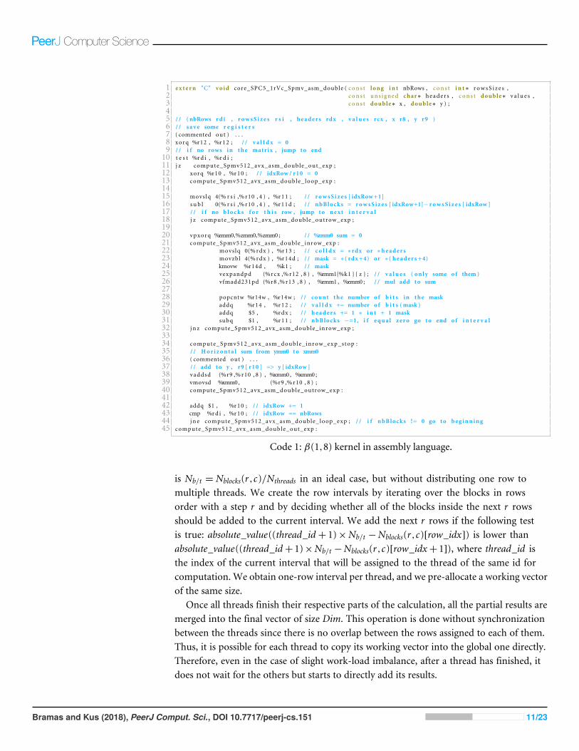
1 ex t e rn "C" void core_SPC5_1rVc_Spmv_asm_double ( c on s t long i n t nbRows , c on s t i n t ∗ r ow s S i z e s ,2 c on s t uns i gned char∗ heade r s , c on s t double∗ v a l u e s ,3 c on s t double∗ x , double∗ y ) ;45 / / ( nbRows rd i , r owsS i z e s r s i , headers rdx , v a l u e s rcx , x r8 , y r9 )6 / / s ave some r e g i s t e r s7 ( commented out ) . . .8 xorq %r12 , %r12 ; / / v a l I d x = 09 / / i f no rows in the matrix , jump to end10 t e s t %rd i , %r d i ;11 j z compute_Spmv512_avx_asm_double_out_exp ;12 xorq %r10 , %r10 ; / / idxRow / r10 = 013 compute_Spmv512_avx_asm_double_loop_exp :1415 movslq 4(% r s i ,%r10 , 4 ) , %r11 ; / / r owsS i z e s [ idxRow+1]16 s u b l 0(% r s i ,%r10 , 4 ) , %r11d ; / / nbBlocks = rowsS i z e s [ idxRow+1]− rowsS i z e s [ idxRow ]17 / / i f no b lock s f o r t h i s row , jump to next i n t e r v a l18 j z compute_Spmv512_avx_asm_double_outrow_exp ;1920 vpxorq %zmm0,%zmm0,%zmm0 ; / / %zmm0 sum = 021 compute_Spmv512_avx_asm_double_inrow_exp :22 movslq 0(%rdx ) , %r13 ; / / c o l I dx = ∗ rdx or ∗headers23 movzbl 4(%rdx ) , %r14d ; / / mask = ∗ ( rdx +4) or ∗ ( headers +4)24 kmovw %r14d , %k1 ; / / mask25 vexpandpd (%rcx ,%r12 , 8 ) , %zmm1{%k1 } { z } ; / / v a l u e s ( only some of them )26 vfmadd231pd (%r8 ,%r13 , 8 ) , %zmm1 , %zmm0 ; / / mul add to sum2728 popcntw %r14w , %r14w ; / / count the number of b i t s in the mask29 addq %r14 , %r12 ; / / v a l I d x += number of b i t s (mask )30 addq $5 , %rdx ; / / headers += 1 ∗ i n t + 1 mask31 subq $1 , %r11 ; / / nbBlocks −=1, i f equa l zero go to end of i n t e r v a l32 j n z compute_Spmv512_avx_asm_double_inrow_exp ;3334 compute_Spmv512_avx_asm_double_ inrow_exp_stop :35 / / Hor i zon ta l sum from ymm0 to xmm036 ( commented out ) . . .37 / / add to y , r9 [ r10 ] => y [ idxRow ]38 vaddsd (%r9 ,%r10 , 8 ) , %xmm0, %xmm0 ;39 vmovsd %xmm0, (%r9 ,%r10 , 8 ) ;40 compute_Spmv512_avx_asm_double_outrow_exp :4142 addq $1 , %r10 ; / / idxRow += 143 cmp %rd i , %r10 ; / / idxRow == nbRows44 j n e compute_Spmv512_avx_asm_double_loop_exp ; / / i f nbBlocks != 0 go to beg inn ing45 compute_Spmv512_avx_asm_double_out_exp :
Code 1: β(1,8) kernel in assembly language.
is Nb/t = Nblocks(r,c)/Nthreads in an ideal case, but without distributing one row tomultiple threads. We create the row intervals by iterating over the blocks in rowsorder with a step r and by deciding whether all of the blocks inside the next r rowsshould be added to the current interval. We add the next r rows if the following testis true: absolute_value((thread_id + 1)×Nb/t −Nblocks(r,c)[row_idx]) is lower thanabsolute_value((thread_id+ 1)×Nb/t −Nblocks(r,c)[row_idx+ 1]), where thread_id isthe index of the current interval that will be assigned to the thread of the same id forcomputation. We obtain one-row interval per thread, and we pre-allocate a working vectorof the same size.
Once all threads finish their respective parts of the calculation, all the partial results aremerged into the final vector of size Dim. This operation is done without synchronizationbetween the threads since there is no overlap between the rows assigned to each of them.Thus, it is possible for each thread to copy its working vector into the global one directly.Therefore, even in the case of slight work-load imbalance, after a thread has finished, itdoes not wait for the others but starts to directly add its results.
Bramas and Kus (2018), PeerJ Comput. Sci., DOI 10.7717/peerj-cs.151 11/23

We attempt to reduce the NUMA effects by splitting the matrix’s arrays values,block_colidx, block_rowptr and block_masks to allocate sub-arrays for each thread inthe memory node that corresponds to the core where it is pinned. There are, however,conceptual disadvantages to this approach since it duplicates thematrix, at least temporarily,in memory during the copy and it ties the data structure and memory distribution to thenumber of threads. The vectors x and y are still allocated by the master thread, and x isaccessed during the computation while y is only accessed during the merge.
PERFORMANCE ANALYSISIn the previous section, a family of sparse matrix formats and their corresponding SpMVkernels has been described. In this section, we show their performance using selectedmatrices from the SuiteSparse Matrix Collection, formerly known as the University ofFlorida Sparse Matrix Collection (Davis & Hu, 2011). We describe our methodology andprovide comparisons between our kernels of different block sizes, and also comparisonswith MKL and CSR5 libraries. The performance comparisons are presented for serial(‘Sequential SpMV performance’) and parallel (‘Parallel SpMV performance’) versions ofalgorithms, respectively.
Hardware/softwareWe used a compute node with two Intel Xeon Platinum 8170 (Skylake) CPUs at 2.10 GHzand 26 cores each, with caches of sizes 32K, 1024K and 36608K, and the GNU compiler6.3. We bind the memory allocation using numaclt –localalloc, and we bind the processesby setting OMP_PROC_BIND=true. As references, we use Intel MKL 2017.2 and the CSR5package taken from the bhSPARSE repository accessed on the 11th of September 2017(https://github.com/bhSPARSE/Benchmark_SpMV_using_CSR5). We obtain a floatingpoint operation per second (FLOPS) measure using the formula 2×NNNZ/T , where Tis the execution time in seconds. The execution time is measured as an average of 16consecutive runs without accessing the matrix before the first run.
Test matricesWe selected matrices that were used in the study (Ye, Calvin & Petiton, 2014) and addedfew more to obtain a diverse set. The matrices labeled Set-A, see Table 1, are used in thecomputation benchmark. Their execution times are also used in our prediction system,which will be introduced in ‘Performance Prediction and Optimal Kernel Selection’.
The user of our library could create the matrix directly using one of our block-basedschemes even though it is more likely to be impossible in many cases due to incompatibilitywith the other parts of the application. If he could, he would be able to choose the mostappropriate block size depending on the expected matrix structure. Otherwise, the user willneed to convert the matrix from a standard CSR format to one of our formats. The timetaken to convert any of the matrices form the Set-A from the CSR format to one of oursis around twice the time of a single SpMV in sequential. For example, for the atmosmoddand bone010, the conversion takes approximately 0.4 and 4 s, and the sequential executionaround 0.2 and 1.5 s, respectively. In a typical scenario, however, many matrix-vector
Bramas and Kus (2018), PeerJ Comput. Sci., DOI 10.7717/peerj-cs.151 12/23
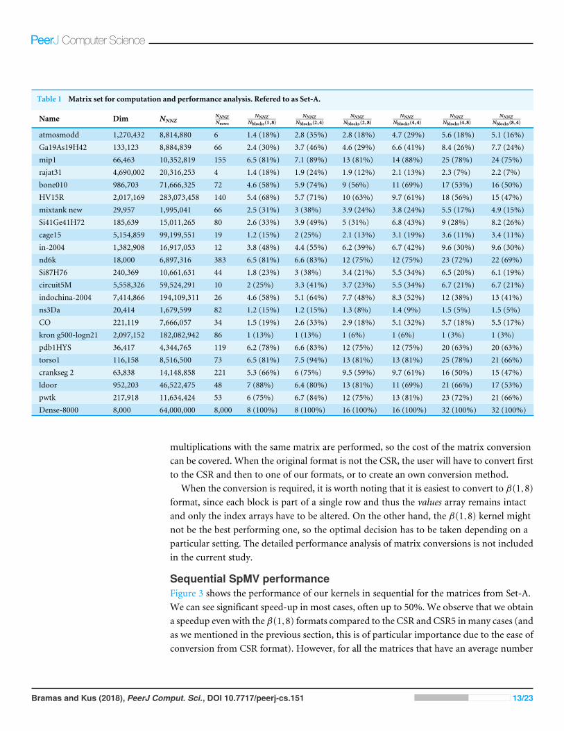
Table 1 Matrix set for computation and performance analysis. Refered to as Set-A.
Name Dim NNNZNNNZNrows
NNNZNblocks(1,8)
NNNZNblocks(2,4)
NNNZNblocks(2,8)
NNNZNblocks(4,4)
NNNZNblocks(4,8)
NNNZNblocks(8,4)
atmosmodd 1,270,432 8,814,880 6 1.4 (18%) 2.8 (35%) 2.8 (18%) 4.7 (29%) 5.6 (18%) 5.1 (16%)Ga19As19H42 133,123 8,884,839 66 2.4 (30%) 3.7 (46%) 4.6 (29%) 6.6 (41%) 8.4 (26%) 7.7 (24%)mip1 66,463 10,352,819 155 6.5 (81%) 7.1 (89%) 13 (81%) 14 (88%) 25 (78%) 24 (75%)rajat31 4,690,002 20,316,253 4 1.4 (18%) 1.9 (24%) 1.9 (12%) 2.1 (13%) 2.3 (7%) 2.2 (7%)bone010 986,703 71,666,325 72 4.6 (58%) 5.9 (74%) 9 (56%) 11 (69%) 17 (53%) 16 (50%)HV15R 2,017,169 283,073,458 140 5.4 (68%) 5.7 (71%) 10 (63%) 9.7 (61%) 18 (56%) 15 (47%)mixtank new 29,957 1,995,041 66 2.5 (31%) 3 (38%) 3.9 (24%) 3.8 (24%) 5.5 (17%) 4.9 (15%)Si41Ge41H72 185,639 15,011,265 80 2.6 (33%) 3.9 (49%) 5 (31%) 6.8 (43%) 9 (28%) 8.2 (26%)cage15 5,154,859 99,199,551 19 1.2 (15%) 2 (25%) 2.1 (13%) 3.1 (19%) 3.6 (11%) 3.4 (11%)in-2004 1,382,908 16,917,053 12 3.8 (48%) 4.4 (55%) 6.2 (39%) 6.7 (42%) 9.6 (30%) 9.6 (30%)nd6k 18,000 6,897,316 383 6.5 (81%) 6.6 (83%) 12 (75%) 12 (75%) 23 (72%) 22 (69%)Si87H76 240,369 10,661,631 44 1.8 (23%) 3 (38%) 3.4 (21%) 5.5 (34%) 6.5 (20%) 6.1 (19%)circuit5M 5,558,326 59,524,291 10 2 (25%) 3.3 (41%) 3.7 (23%) 5.5 (34%) 6.7 (21%) 6.7 (21%)indochina-2004 7,414,866 194,109,311 26 4.6 (58%) 5.1 (64%) 7.7 (48%) 8.3 (52%) 12 (38%) 13 (41%)ns3Da 20,414 1,679,599 82 1.2 (15%) 1.2 (15%) 1.3 (8%) 1.4 (9%) 1.5 (5%) 1.5 (5%)CO 221,119 7,666,057 34 1.5 (19%) 2.6 (33%) 2.9 (18%) 5.1 (32%) 5.7 (18%) 5.5 (17%)kron g500-logn21 2,097,152 182,082,942 86 1 (13%) 1 (13%) 1 (6%) 1 (6%) 1 (3%) 1 (3%)pdb1HYS 36,417 4,344,765 119 6.2 (78%) 6.6 (83%) 12 (75%) 12 (75%) 20 (63%) 20 (63%)torso1 116,158 8,516,500 73 6.5 (81%) 7.5 (94%) 13 (81%) 13 (81%) 25 (78%) 21 (66%)crankseg 2 63,838 14,148,858 221 5.3 (66%) 6 (75%) 9.5 (59%) 9.7 (61%) 16 (50%) 15 (47%)ldoor 952,203 46,522,475 48 7 (88%) 6.4 (80%) 13 (81%) 11 (69%) 21 (66%) 17 (53%)pwtk 217,918 11,634,424 53 6 (75%) 6.7 (84%) 12 (75%) 13 (81%) 23 (72%) 21 (66%)Dense-8000 8,000 64,000,000 8,000 8 (100%) 8 (100%) 16 (100%) 16 (100%) 32 (100%) 32 (100%)
multiplications with the same matrix are performed, so the cost of the matrix conversioncan be covered. When the original format is not the CSR, the user will have to convert firstto the CSR and then to one of our formats, or to create an own conversion method.
When the conversion is required, it is worth noting that it is easiest to convert to β(1,8)format, since each block is part of a single row and thus the values array remains intactand only the index arrays have to be altered. On the other hand, the β(1,8) kernel mightnot be the best performing one, so the optimal decision has to be taken depending on aparticular setting. The detailed performance analysis of matrix conversions is not includedin the current study.
Sequential SpMV performanceFigure 3 shows the performance of our kernels in sequential for the matrices from Set-A.We can see significant speed-up in most cases, often up to 50%. We observe that we obtaina speedup even with the β(1,8) formats compared to the CSR and CSR5 inmany cases (andas we mentioned in the previous section, this is of particular importance due to the ease ofconversion from CSR format). However, for all the matrices that have an average number
Bramas and Kus (2018), PeerJ Comput. Sci., DOI 10.7717/peerj-cs.151 13/23

Computing the Sparse Matrix Vector Product using Block-Based Kernels Without Zero Padding
matrix sparsity pattern). In fact, if we look to the Dense-8000 matrix where all the blocks are completely317
filled, the performance is not very different from one kernel to the other. For instance, there are more values318
per block in the β(8, 4) then in the β(4, 8) storage only for indochina-2004 matrix, which means that it did319
not help to capture 8 rows per block instead of 8 columns.320
atmosmodd
Ga19A
s19H
42
mip1
rajat31
bone010
HV15R
mixtank
new
Si41Ge41H
72
0
2
4
0.9
9 1.0
4
1.3
9
0.8
7
1.3
8
1.4
2
0.7
7
1.1
1
1.1
8 1.1
8 1.3
9
1.0
4
1.3
9
1.4
2
0.8
2
1.2
1.2
1.2
2 1.4
1
0.9
4
1.3
9
1.4
1
1.1
3
1.2
4
1.0
8
1.1
8
1.4
6
0.8
3
1.4
1
1.4
3
1.1
1.2
1
1.2
3
1.3
1.4
5
0.8
3
1.4
2
1.4
2
0.9
8
1.3
3
1.1
6
1.2
2
1.4
8
0.6
9
1.4
2
1.4
3
0.9
8
1.2
5
0.9
5 1.0
3
1.4
4
0.5
4
1.3
9
1.4
2
0.7
0
1.0
8
GFlop/s
MKL CSR CSR5 SPC5 β(1, 8) test SPC5 β(2, 4) test SPC5 β(2, 4)
SPC5 β(2, 8) SPC5 β(4, 4) SPC5 β(4, 8) SPC5 β(8, 4)
cage15
in-2004
nd6k
Si87H76
circuit5M
indochina-2004
ns3D
a
CO
0
2
4
0.7
6
1.0
1
1.3
7
0.9
0
1.0
6 1.1
4
0.3
7 0.8
1
0.8
3
1.0
4
1.3
8
1.0
2
1.2 1.1
4
0.2
2
0.9
6
0.9
5 1.3
1
1.4
1
1.0
7
1.2
3 1.3
1
0.5
7 0.9
8
0.8
5 1.3
1.5
1
1.1
7 1.3
1
0.4
1
0.9
0
0.9
5 1.3
3
1.4
5
1.2
2
1.2
9 1.3
1
0.3
6
1.1
6
0.8
4 1.3
1.5
2
1.0
7
1.2
1 1.2
8
0.2
8
0.9
9
0.6
9
1.1
8
1.4
4
0.8
8
1.1
2 1.2
0.2
0.8
1
GFlop/s
kron
g500-logn21
pdb1HYS
torso1
crankseg
2
ldoor
pwtk
Dense-8000
0
2
4
0.7
2
1.4
2
1.4
1.3
4
1.4
5
1.3
5
1.3
5
0.7
2
1.5
8
1.4
4
1.3
6
1.4
5
1.3
8
1.3
6
0.4
8
1.5
8
1.4
6
1.3
8
1.4
3
1.4
1
1.3
6
0.3
5
1.6
9
1.5
1
1.4
1
1.4
8
1.4
4
1.3
8
0.5
1.6
6
1.4
7
1.3
8
1.4
5
1.4
4
1.3
8
0.3
9
1.7
1.5
3
1.4
1.4
8
1.4
6
1.3
9
0.4
3
1.6
3
1.4
4
1.3
5
1.4
2
1.4
1.3
8
Matrices
GFlop/s
Figure 3: Performance in Giga Flop per second for sequential computation in double precision for the MKLCSR, the CSR5 and our SPC5 kernels. Speedup of SPC5 against the better of MKL CSR and CSR5 isshown above the bars.
4.4 Parallel SpMV Performance321
Figure 4 shows the performance of parallel versions of all investigated kernels using 52 cores for the matrices322
from the Set-A. The parallel version of MKL CSR is not able to take significant advantage of this number of323
threads, and it is faster only for kron g500-logn21 matrix. The CSR5 package is efficient especially when the324
12
PeerJ Comput. Sci. reviewing PDF | (CS-2018:01:23006:1:1:NEW 5 Mar 2018)
Manuscript to be reviewedComputer Science
Figure 3 Performance in Giga Flop per second for sequential computation in double precision for theMKL CSR, the CSR5 and our SPC5 kernels. Speedup of SPC5 against the better of MKL CSR and CSR5 isshown above the bars.
Full-size DOI: 10.7717/peerjcs.151/fig-3
of non-zero values per block of corresponding storage below 2, the β(1,8) is more likelyto be slower than the CSR (with some exceptions, e.g., for the mixtank new the average is2.5 and β(1,8) is still slower). For the other blocks sizes, we obtain a similar behavior, i.e.,if there are insufficient values per block, the performance decreases. The worse case is forthe ns3Da and kron g500-logn21 matrices, and we see from Table 1 that the blocks remainunfilled for all the considered storages. That hurts the performance of our block-basedkernels, since 8 or 4 values still have to be loaded from x, even though only one value isuseful, and large width arithmetic operations (multiplication and addition of vectors) stillhave to be called.
For the β(2,4) storage, the test-based scheme provides a speedup only for rajat31. Forother formats, we see that the performance is mainly a matter of the average number
Bramas and Kus (2018), PeerJ Comput. Sci., DOI 10.7717/peerj-cs.151 14/23

Computing the Sparse Matrix Vector Product using Block-Based Kernels Without Zero Padding
matrix’s structure makes it difficult to achieve high flop-rate. In these cases it has a performance similar or325
higher than our block-based kernels. All our kernels have very similar performances. By comparing Figure 4326
with Table 1 we can observe that the NUMA optimization gives noticeable speedup for large matrices (shown327
as the dark part of bars in Figure 4. Indeed, when a matrix is allocated on a single memory socket, any328
access by threads on a different socket is very expensive. This might not be a severe problem if the matrix329
(or at least the part used by the threads) fits in the L3 cache. Then, only the first access is costly, especially330
when the data is read-only. On the other hand, if the matrix does not fit in the L3 cache, multiple expensive331
memory transfers will take place during the computation without any possibility for the CPU to hide them.332
atmosmodd
Ga19A
s19H
42
mip1
rajat31
bone010
HV15R
mixtank
new
Si41Ge41H
72
0
50
100
150
1.5
2
1.1
8
1.1
6
1.7
7
1.1
1
1.1
2
1.0
8 2.3
1
1.8
5
1.4
8 1.1
5
1.8
6
1.2
7
1.3
1
1.2
5 2.6
4
1.9
6
1.4
5 1.1
5
1.8
2
1.2
7
1.3
2
1.5
9
2.7
8
1.6
3
1.1
5
1.1
4
1.7
8
1.4
9
1.4
1.3
1
2.5
8
2.0
3
1.4
4
1.2
6
1.8 1.5
1
1.4
1.2
2.9
9
1.8
1.4
4 1.1
5
1.7
4
1.5
2
1.4
6
1.2
2.7
6
1.4
8
1.2
1.1
3
1.6
6
1.5
8
1.4
2 0.9
0
2.4
4
atmosmodd
Ga19A
s19H
42
mip1
rajat31
bone010
HV15R
mixtank
new
Si41Ge41H
72
0
50
100
150
GFlop/s
MKL CSR CSR5 SPC5 β(1, 8) test SPC5 β(2, 4) test SPC5 β(2, 4)
SPC5 β(2, 8) SPC5 β(4, 4) SPC5 β(4, 8) SPC5 β(8, 4)
cage15
in-2004
nd6k
Si87H76
circuit5M
indochina-2004
ns3D
a
CO
0
50
100
150
1.4
3 2.6
1.4
7
1.9
8
1.1
5
2.4
9
0.4
6
0.7
5
2.2
4
2.7
2
1.4
4
2.3
5
1.8
2
2.6
9
0.3
0.9
3
2.3
9
2.7
9
1.5
3
2.6
7
1.8
3
2.7
8
0.6
9
0.9
8
2.4
7
2.8
8
1.6
1
2.2
3
1.4
8 2.8
3
0.5
0.8
3
2.4
7
2.8
6
1.6
2.8
6
2.0
9
2.8
9
0.4
7
1.2
4
2.4
9
2.6
7
1.8
2.5
5
1.6
9
2.7
0.3
4
0.8
6
2.3
2
2.7
1
1.6
9
2.0
8
2.0
1
2.6
5
0.2
7
0.8
2
cage15
in-2004
nd6k
Si87H76
circuit5M
indochina-2004
ns3D
a
CO
0
50
100
150
GFlop/s
kron
g500-logn21
pdb1HYS
torso1
crankseg
2
ldoor
pwtk
Dense-8000
0
50
100
150
1.0
8
1.6
4
1.4
6
4.9
7
3.9
7
4.0
6
4.3
1.2
1
1.8
1
1.5
5
5.0
5
3.9
6
4.0
6
4.7
3
0.8
6
1.8
8
1.5
8
5.0
8
3.9
7
4.1
4.7
3
0.6
6
1.9
4
1.6
5.1
3
4.1
2
4.4
9
4.8
9
0.8
0
1.8
4
1.5
8
5.1
4
4.1
1
4.2
2
4.8
8
0.6
9
2.0
8
1.6
5.3
6
4.1
7
4.6
4
4.9
6
0.6
6
1.8
4
1.3
1
5.0
6
4.1
4
4.2
5
4.9
2
kron
g500-logn21
pdb1HYS
torso1
crankseg
2
ldoor
pwtk
Dense-8000
0
50
100
150
Matrices
GFlop/s
Figure 4: Performance in Giga Flop per second in double precision for the parallel implementations of MKLCSR, the CSR5 and our SPC5 kernels, all using 52 threads. Each bar shows the performance without NUMAoptimization (light) and with NUMA optimization (dark). Speedup of SPC5 with NUMA optimizationsagainst the better of MKL CSR and CSR5 is shown above the bars.
13
PeerJ Comput. Sci. reviewing PDF | (CS-2018:01:23006:1:1:NEW 5 Mar 2018)
Manuscript to be reviewedComputer Science
Figure 4 Performance in Giga Flop per second in double precision for the parallel implementations ofMKL CSR, the CSR5 and our SPC5 kernels, all using 52 threads. Each bar shows the performance with-out NUMA optimization (light) and with NUMA optimization (dark). Speedup of SPC5 with NUMA op-timizations against the better of MKL CSR and CSR5 is shown above the bars.
Full-size DOI: 10.7717/peerjcs.151/fig-4
of values per block (so related to the matrix sparsity pattern). In fact, if we look to theDense-8000 matrix where all the blocks are completely filled, the performance is not verydifferent from one kernel to the other. For instance, there are more values per block in theβ(8,4) then in the β(4,8) storage only for indochina-2004matrix, which means that it didnot help to capture 8 rows per block instead of 8 columns.
Parallel SpMV performanceFigure 4 shows the performance of parallel versions of all investigated kernels using 52cores for the matrices from the Set-A. The parallel version of MKL CSR is not able to takesignificant advantage of this number of threads, and it is faster only for kron g500-logn21matrix. The CSR5 package is efficient especially when the matrix’s structure makes it
Bramas and Kus (2018), PeerJ Comput. Sci., DOI 10.7717/peerj-cs.151 15/23

difficult to achieve high flop-rate. In these cases it has a performance similar or higher thanour block-based kernels. All our kernels have very similar performances. By comparing Fig.4 with Table 1 we can observe that the NUMA optimization gives noticeable speedup forlarge matrices (shown as the dark part of bars in Fig. 4. Indeed, when a matrix is allocatedon a single memory socket, any access by threads on a different socket is very expensive.This might not be a severe problem if thematrix (or at least the part used by the threads) fitsin the L3 cache. Then, only the first access is costly, especially when the data is read-only.On the other hand, if the matrix does not fit in the L3 cache, multiple expensive memorytransfers will take place during the computation without any possibility for the CPU tohide them.
PERFORMANCE PREDICTION AND OPTIMAL KERNELSELECTIONIn the previous section, we compared our method with MKL and CSR5 and showed asignificant speed-up for most matrices using any block size. The question that arises,however, is what block size should the user choose to maximize the performance. As itcan be seen in Figs. 3 and 4, the performance of individual kernels for different block sizesvaries and the best option depends on the matrix.
If the user applies the presented library on many matrices with a similar structure, it isquite likely that he can find an optimal kernel in just several trials. If, however, the userdoes not have any idea about the structure of the given matrix and no experience withexecution times of individual kernels, some decision-making process should be supplied.There are many possible approaches to address this challenging problem. If it should beusable, it needs to be computationally cheap, without conversion of the matrix, yet stillable to advise the user about the block size to take.
In the following subsection, we describe several possible approaches towards thisproblem. The matrices from the Set-A listed in Table 1 are used to fine-tune the predictionmethod. To assess each of the methods, we introduce new, independent set of matriceslabeled Set-B and listed in Table 2.
Performance polynomial interpolation (sequential)Figure 5 shows the dependence of kernel performance on an average number of NNZper block. Each kernel-matrix combination is plotted as a single dot. One can clearly seea correlation between the two quantities, slightly different for each kernel. Polynomialinterpolation has been done for each kernel using the matrices from Set-A and its resultsare shown in Fig. 5.
The Avg.NNZ/blocks numbers can be obtained without converting the matrices intoa block-based storage. This can be used to roughly estimate the performance of eachindividual kernel. It is clear, however, that even within the matrix set used for interpolation,there are matrices with a significantly different performance from the one suggested bythe interpolation curve. This difference illustrates the fact that the Avg.NNZ/block metricis a very high-level information that hides all the memory accesses patterns, which canbe different depending on the positions of the blocks and their individual structure. If
Bramas and Kus (2018), PeerJ Comput. Sci., DOI 10.7717/peerj-cs.151 16/23
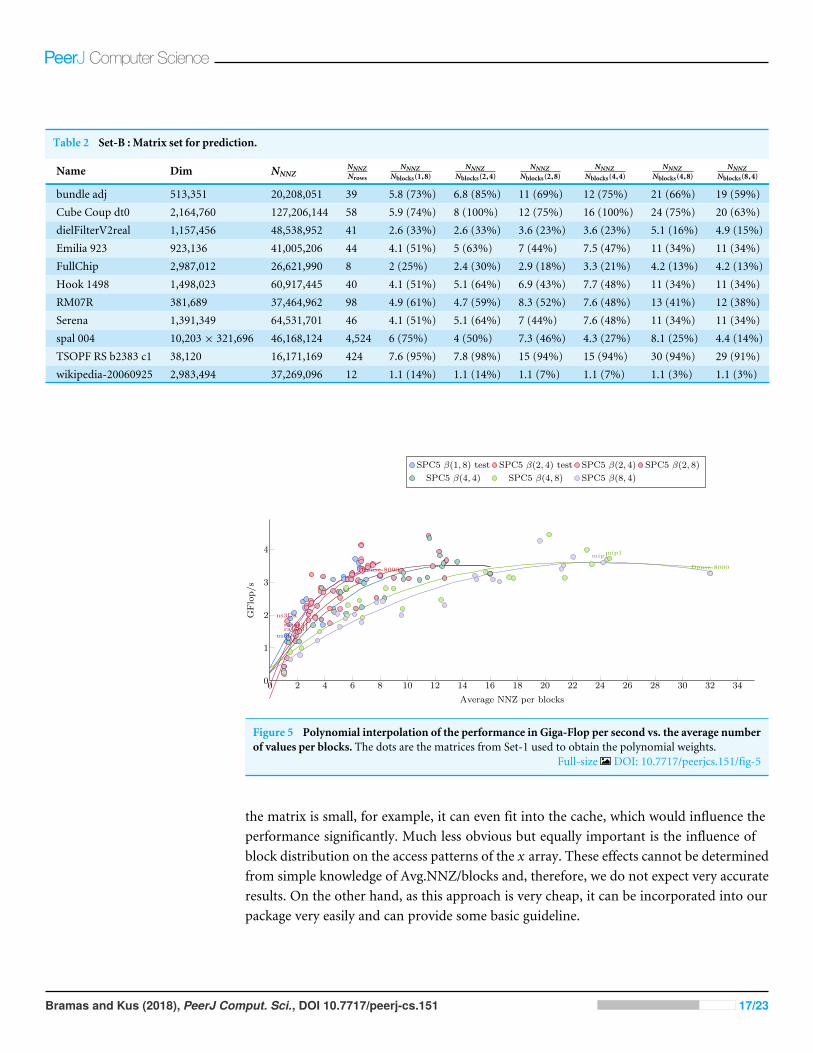
Table 2 Set-B : Matrix set for prediction.
Name Dim NNNZNNNZNrows
NNNZNblocks(1,8)
NNNZNblocks(2,4)
NNNZNblocks(2,8)
NNNZNblocks(4,4)
NNNZNblocks(4,8)
NNNZNblocks(8,4)
bundle adj 513,351 20,208,051 39 5.8 (73%) 6.8 (85%) 11 (69%) 12 (75%) 21 (66%) 19 (59%)Cube Coup dt0 2,164,760 127,206,144 58 5.9 (74%) 8 (100%) 12 (75%) 16 (100%) 24 (75%) 20 (63%)dielFilterV2real 1,157,456 48,538,952 41 2.6 (33%) 2.6 (33%) 3.6 (23%) 3.6 (23%) 5.1 (16%) 4.9 (15%)Emilia 923 923,136 41,005,206 44 4.1 (51%) 5 (63%) 7 (44%) 7.5 (47%) 11 (34%) 11 (34%)FullChip 2,987,012 26,621,990 8 2 (25%) 2.4 (30%) 2.9 (18%) 3.3 (21%) 4.2 (13%) 4.2 (13%)Hook 1498 1,498,023 60,917,445 40 4.1 (51%) 5.1 (64%) 6.9 (43%) 7.7 (48%) 11 (34%) 11 (34%)RM07R 381,689 37,464,962 98 4.9 (61%) 4.7 (59%) 8.3 (52%) 7.6 (48%) 13 (41%) 12 (38%)Serena 1,391,349 64,531,701 46 4.1 (51%) 5.1 (64%) 7 (44%) 7.6 (48%) 11 (34%) 11 (34%)spal 004 10,203× 321,696 46,168,124 4,524 6 (75%) 4 (50%) 7.3 (46%) 4.3 (27%) 8.1 (25%) 4.4 (14%)TSOPF RS b2383 c1 38,120 16,171,169 424 7.6 (95%) 7.8 (98%) 15 (94%) 15 (94%) 30 (94%) 29 (91%)wikipedia-20060925 2,983,494 37,269,096 12 1.1 (14%) 1.1 (14%) 1.1 (7%) 1.1 (7%) 1.1 (3%) 1.1 (3%)
Computing the Sparse Matrix Vector Product using Block-Based Kernels Without Zero Padding
0 2 4 6 8 10 12 14 16 18 20 22 24 26 28 30 32 340
1
2
3
4
ns3Da
Dense-8000
rajat31
ns3Da
rajat31
mip1
Dense-8000
mip1
Average NNZ per blocks
GFlop/s
SPC5 β(1, 8) test SPC5 β(2, 4) test SPC5 β(2, 4) SPC5 β(2, 8)
SPC5 β(4, 4) SPC5 β(4, 8) SPC5 β(8, 4)
Figure 5: Polynomial interpolation of the performance in Giga-Flop per second vs. the average number ofvalues per blocks. The dots are the matrices from Set-1 used to obtain the polynomial weights.
provide the objectively best kernel and its speed, the recommended kernel and its estimated and real speed368
and, finally, the difference between the best and recommended kernels speed.369
If the selected kernel is the optimal one, then Best kernel has the same value as Selected kernel and Speed370
difference is zero. We see that the method selects the best kernels or kernels that have very close performance371
in most cases, even though the performance estimations as such are not always completely accurate. In other372
words, the values in columns Best kernel speed and Selected kernel predicted speed are in most cases quite373
similar, but there are general differences between values in columns Selected kernel predicted speed and Real374
speed of selected kernel.375
For some matrices, all kernels have very similar performance and thus, even if the prediction is not376
accurate and a random kernel is selected, its performance is actually not far from the optimal one. For other377
matrices, it seems that if they have a special structure that makes the performance far from the one given378
by the interpolation curves, this is the case for all kernels and so the kernel recommendation is finally good.379
Of course, one could design a specific sparsity pattern in order to make the prediction fail, but it seems that380
this simple and cheap prediction system works reasonably well for real-world matrices.381
5.2 Parallel Performance Estimation382
Similarly, as we have done for the sequential kernels in the last section, we attempt to estimate the perfor-383
mance of parallel kernels in order to advise the user about the best block size to choose for a given matrix384
before the matrix is converted into a block-based format. The situation is, however, more complicated since385
the performance of the kernels will depend on another parameter: the number of threads, which will be386
used. Thus, we perform a non-linear 2D regression of performance based on two parameters: the number387
of threads and the average values per block. We use performance results obtained for matrices from Set-A388
using 1, 4, 16, 32 and 52 threads for each kernel.389
The results are then used to estimate (by interpolation) the performance of individual kernels for a given390
setup. The results of interpolation used on both Set-A and independent Set-B are shown in Figure 6. We391
show in Figure 6A when this strategy leads to an optimal kernel selection. In Figure 6B, we show what is392
the real performance difference between the kernel advised and the one that is actually the fastest, and in393
Figure 6C, we show the prediction difference for the selected kernel/block size. We observe that the approach394
15
PeerJ Comput. Sci. reviewing PDF | (CS-2018:01:23006:1:1:NEW 5 Mar 2018)
Manuscript to be reviewedComputer Science
Figure 5 Polynomial interpolation of the performance in Giga-Flop per second vs. the average numberof values per blocks. The dots are the matrices from Set-1 used to obtain the polynomial weights.
Full-size DOI: 10.7717/peerjcs.151/fig-5
the matrix is small, for example, it can even fit into the cache, which would influence theperformance significantly. Much less obvious but equally important is the influence ofblock distribution on the access patterns of the x array. These effects cannot be determinedfrom simple knowledge of Avg.NNZ/blocks and, therefore, we do not expect very accurateresults. On the other hand, as this approach is very cheap, it can be incorporated into ourpackage very easily and can provide some basic guideline.
Bramas and Kus (2018), PeerJ Comput. Sci., DOI 10.7717/peerj-cs.151 17/23

To select a kernel, we perform the following steps. From a given matrix, we firstcompute the Avg.NNZ/blocks for the sizes that correspond to our formats. Then, we usethe estimation formulas plotted in Fig. 5 to have an estimation of the performance for eachkernel. Finally, we select the kernel with the highest estimated performance as the one touse.
We can assess a quality of the prediction system using data shown in Table 3. For eachmatrix, we provide the objectively best kernel and its speed, the recommended kernel andits estimated and real speed and, finally, the difference between the best and recommendedkernels speed.
If the selected kernel is the optimal one, then Best kernel has the same value as Selectedkernel and Speed difference is zero.We see that the method selects the best kernels or kernelsthat have very close performance in most cases, even though the performance estimationsas such are not always completely accurate. In other words, the values in columns Bestkernel speed and Selected kernel predicted speed are in most cases quite similar, but thereare general differences between values in columns Selected kernel predicted speed and Realspeed of selected kernel.
For some matrices, all kernels have very similar performance and thus, even if theprediction is not accurate and a random kernel is selected, its performance is actually notfar from the optimal one. For other matrices, it seems that if they have a special structurethat makes the performance far from the one given by the interpolation curves, this is thecase for all kernels and so the kernel recommendation is finally good. Of course, one coulddesign a specific sparsity pattern in order to make the prediction fail, but it seems that thissimple and cheap prediction system works reasonably well for real-world matrices.
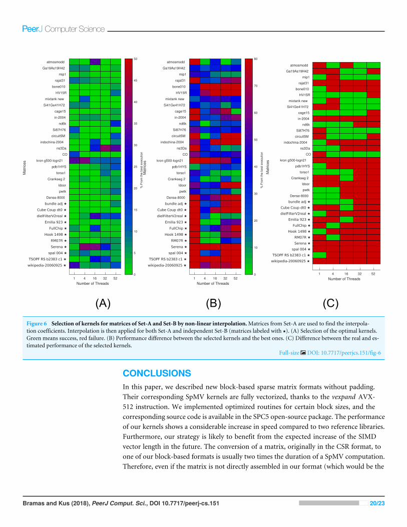
Parallel performance estimationSimilarly, as we have done for the sequential kernels in the last section, we attempt toestimate the performance of parallel kernels in order to advise the user about the bestblock size to choose for a given matrix before the matrix is converted into a block-basedformat. The situation is, however, more complicated since the performance of the kernelswill depend on another parameter: the number of threads, which will be used. Thus, weperform a non-linear 2D regression of performance based on two parameters: the numberof threads and the average values per block. We use performance results obtained formatrices from Set-A using 1, 4, 16, 32 and 52 threads for each kernel.
The results are then used to estimate (by interpolation) the performance of individualkernels for a given setup. The results of interpolation used on both Set-A and independentSet-B are shown in Fig. 6. We show in Fig. 6A when this strategy leads to an optimal kernelselection. In Fig. 6B, we show what is the real performance difference between the kerneladvised and the one that is actually the fastest, and in Fig. 6C, we show the predictiondifference for the selected kernel/block size. We observe that the approach does not selectthe optimal kernels in most cases, but we can also see that the performance provided bythe selected kernels are close to the optimal ones (less than 10 percent difference in mostcases). Similarly, as for the polynomial interpolation in sequential, this is true despite theperformance estimation not being accurate.
Bramas and Kus (2018), PeerJ Comput. Sci., DOI 10.7717/peerj-cs.151 18/23
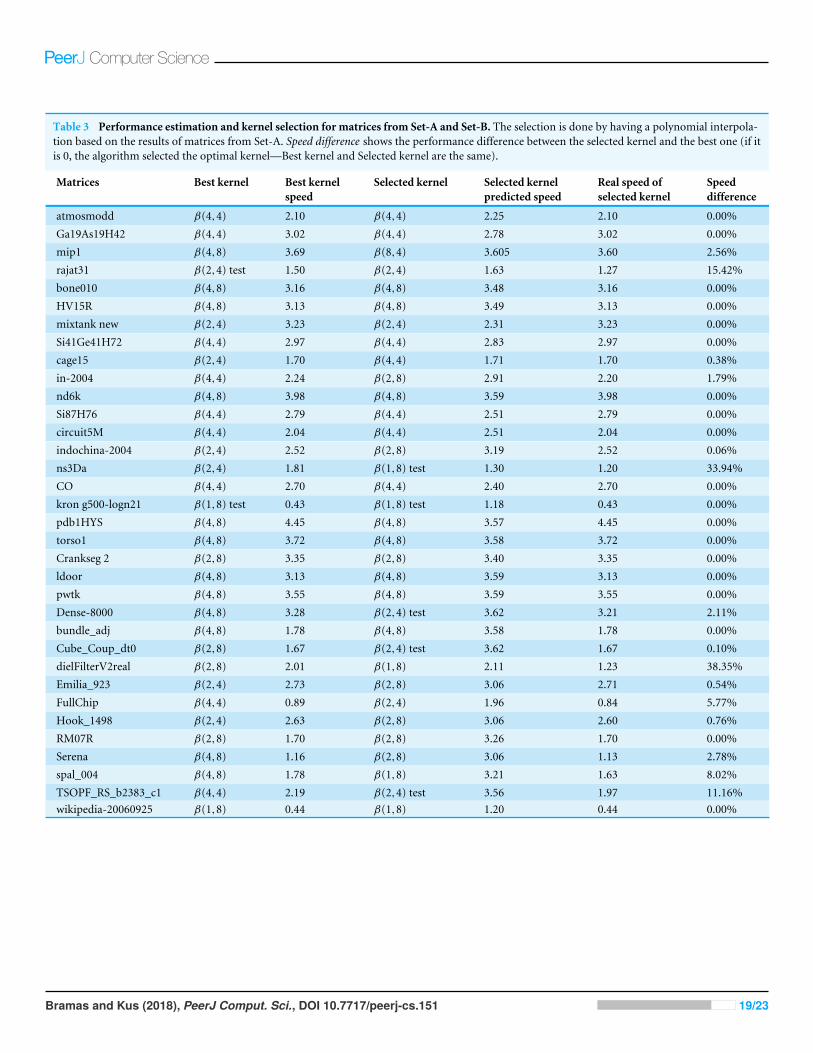
Table 3 Performance estimation and kernel selection for matrices from Set-A and Set-B. The selection is done by having a polynomial interpola-tion based on the results of matrices from Set-A. Speed difference shows the performance difference between the selected kernel and the best one (if itis 0, the algorithm selected the optimal kernel—Best kernel and Selected kernel are the same).
Matrices Best kernel Best kernelspeed
Selected kernel Selected kernelpredicted speed
Real speed ofselected kernel
Speeddifference
atmosmodd β(4,4) 2.10 β(4,4) 2.25 2.10 0.00%Ga19As19H42 β(4,4) 3.02 β(4,4) 2.78 3.02 0.00%mip1 β(4,8) 3.69 β(8,4) 3.605 3.60 2.56%rajat31 β(2,4) test 1.50 β(2,4) 1.63 1.27 15.42%bone010 β(4,8) 3.16 β(4,8) 3.48 3.16 0.00%HV15R β(4,8) 3.13 β(4,8) 3.49 3.13 0.00%mixtank new β(2,4) 3.23 β(2,4) 2.31 3.23 0.00%Si41Ge41H72 β(4,4) 2.97 β(4,4) 2.83 2.97 0.00%cage15 β(2,4) 1.70 β(4,4) 1.71 1.70 0.38%in-2004 β(4,4) 2.24 β(2,8) 2.91 2.20 1.79%nd6k β(4,8) 3.98 β(4,8) 3.59 3.98 0.00%Si87H76 β(4,4) 2.79 β(4,4) 2.51 2.79 0.00%circuit5M β(4,4) 2.04 β(4,4) 2.51 2.04 0.00%indochina-2004 β(2,4) 2.52 β(2,8) 3.19 2.52 0.06%ns3Da β(2,4) 1.81 β(1,8) test 1.30 1.20 33.94%CO β(4,4) 2.70 β(4,4) 2.40 2.70 0.00%kron g500-logn21 β(1,8) test 0.43 β(1,8) test 1.18 0.43 0.00%pdb1HYS β(4,8) 4.45 β(4,8) 3.57 4.45 0.00%torso1 β(4,8) 3.72 β(4,8) 3.58 3.72 0.00%Crankseg 2 β(2,8) 3.35 β(2,8) 3.40 3.35 0.00%ldoor β(4,8) 3.13 β(4,8) 3.59 3.13 0.00%pwtk β(4,8) 3.55 β(4,8) 3.59 3.55 0.00%Dense-8000 β(4,8) 3.28 β(2,4) test 3.62 3.21 2.11%bundle_adj β(4,8) 1.78 β(4,8) 3.58 1.78 0.00%Cube_Coup_dt0 β(2,8) 1.67 β(2,4) test 3.62 1.67 0.10%dielFilterV2real β(2,8) 2.01 β(1,8) 2.11 1.23 38.35%Emilia_923 β(2,4) 2.73 β(2,8) 3.06 2.71 0.54%FullChip β(4,4) 0.89 β(2,4) 1.96 0.84 5.77%Hook_1498 β(2,4) 2.63 β(2,8) 3.06 2.60 0.76%RM07R β(2,8) 1.70 β(2,8) 3.26 1.70 0.00%Serena β(4,8) 1.16 β(2,8) 3.06 1.13 2.78%spal_004 β(4,8) 1.78 β(1,8) 3.21 1.63 8.02%TSOPF_RS_b2383_c1 β(4,4) 2.19 β(2,4) test 3.56 1.97 11.16%wikipedia-20060925 β(1,8) 0.44 β(1,8) 1.20 0.44 0.00%
Bramas and Kus (2018), PeerJ Comput. Sci., DOI 10.7717/peerj-cs.151 19/23
1 4 16 32 52
Number of Threads
Dense-8000
pwtk
ldoor
Crankseg 2
torso1
pdb1HYS
kron g500-logn21
CO
ns3Da
indochina-2004
circuit5M
Si87H76
nd6k
in-2004
cage15
Si41Ge41H72
mixtank new
HV15R
bone010
rajat31
mip1
Ga19As19H42
atmosmodd
Matr
ices
0
5
10
15
20
25
30
35
40
45
50
% F
rom
the b
est execution
1 4 16 32 52
Number of Threads
Dense-8000
pwtk
ldoor
Crankseg 2
torso1
pdb1HYS
kron g500-logn21
CO
ns3Da
indochina-2004
circuit5M
Si87H76
nd6k
in-2004
cage15
Si41Ge41H72
mixtank new
HV15R
bone010
rajat31
mip1
Ga19As19H42
atmosmodd
Matr
ices
0
10
20
30
40
50
60
70
80
% F
rom
the b
est execution
1 4 16 32 52
Number of Threads
Dense-8000
pwtk
ldoor
Crankseg 2
torso1
pdb1HYS
kron g500-logn21
CO
ns3Da
indochina-2004
circuit5M
Si87H76
nd6k
in-2004
cage15
Si41Ge41H72
mixtank new
HV15R
bone010
rajat31
mip1
Ga19As19H42
atmosmodd
Matr
ices
(A) (B) (C)Figure 6 Selection of kernels for matrices of Set-A and Set-B by non-linear interpolation.Matrices from Set-A are used to find the interpola-tion coefficients. Interpolation is then applied for both Set-A and independent Set-B (matrices labeled with ?). (A) Selection of the optimal kernels.Green means success, red failure. (B) Performance difference between the selected kernels and the best ones. (C) Difference between the real and es-timated performance of the selected kernels.
Full-size DOI: 10.7717/peerjcs.151/fig-6
CONCLUSIONSIn this paper, we described new block-based sparse matrix formats without padding.Their corresponding SpMV kernels are fully vectorized, thanks to the vexpand AVX-512 instruction. We implemented optimized routines for certain block sizes, and thecorresponding source code is available in the SPC5 open-source package. The performanceof our kernels shows a considerable increase in speed compared to two reference libraries.Furthermore, our strategy is likely to benefit from the expected increase of the SIMDvector length in the future. The conversion of a matrix, originally in the CSR format, toone of our block-based formats is usually two times the duration of a SpMV computation.Therefore, even if the matrix is not directly assembled in our format (which would be the
Bramas and Kus (2018), PeerJ Comput. Sci., DOI 10.7717/peerj-cs.151 20/23

ideal case, but it might be cumbersome since it usually requires changes in the user code),conversion can be justified, e.g., in the case of iterative methods, where many SpMVs areperformed. Moreover, for the β(1,8) format, the array of values is unchanged, and onlyan extra array to store the blocks’ masks is needed, compared to the CSR storage. Since, atthe same time, the length of colidx array is reduced, block storage leads to smaller memoryrequirements. We have also shown, that when used in parallel, our algorithm can furtherbenefit significantly from reducing the NUMA effect by splitting the arrays, particularlyfor large matrices. This approach, however, has some drawbacks. It splits the arrays for agiven thread configuration so that later, modifications or accesses to the entries becomemore complicated or even more expensive within some codes. For this reason, we providetwo variants of kernels, letting the user to choose whether to optimize for NUMA effectsor not, and we show the performance of both.
The kernels provided by our library are usually significantly faster than the competinglibraries. To use the library to its full extent, however, it is important for the user to predictwhich format (block size) is the most appropriate for a given matrix. This is why we alsoprovide techniques to find the optimal kernels using simple interpolation to be used incases, when the user is unable to choose based on his own knowledge or experience. Theperformance estimate is usually not completely accurate, but the selected format/kernel isvery close to the optimal one, which makes it a reliable method.
In the future, wewould like to developmore sophisticated best kernel predictionmethodswith multiple inputs, such as statistics on the blocks and some hardware properties, thecache size, the memory bandwidth, etc. However, this will require having access to variousSkylake-based hardware and running large benchmark suites. In addition, we would like tofind a way to incorporate such methods in our package without increasing the dependencyfootprint. At the optimization level, we would like, among other things, to assess thebenefit and cost of duplicating the x vector on every memory node within the parallelcomputation.
ADDITIONAL INFORMATION AND DECLARATIONS
FundingThe authors received no funding for this work.
Competing InterestsBerenger Bramas is a researcher at MPCDF. Pavel Kus is a researcher at MPCDF.
Author Contributions• Bérenger Bramas and Pavel Kus conceived and designed the experiments, performed theexperiments, analyzed the data, contributed reagents/materials/analysis tools, preparedfigures and/or tables, performed the computation work, approved the final draft.
Data AvailabilityThe following information was supplied regarding data availability:
GitHub: https://gitlab.mpcdf.mpg.de/bbramas/spc5
Bramas and Kus (2018), PeerJ Comput. Sci., DOI 10.7717/peerj-cs.151 21/23

REFERENCESBarrett R, Berry MW, Chan TF, Demmel J, Donato J, Dongarra J, Eijkhout V, Pozo
R, Romine C, Van der Vorst H. 1994. Templates for the solution of linear systems:building blocks for iterative methods. Vol. 43. Philadelphia: Siam.
Bramas B. 2016. Optimization and parallelization of the boundary element method forthe wave equation in time domain. PhD thesis, Université de Bordeaux.
Buluc A,Williams S, Oliker L, Demmel J. 2011. Reduced-bandwidth multithreadedalgorithms for sparse matrix-vector multiplication. In: Parallel & distributedprocessing symposium (IPDPS), 2011 IEEE international. Piscataway: IEEE, 721–733.
Cuthill E, McKee J. 1969. Reducing the bandwidth of sparse symmetric matrices. In:Proceedings of the 1969 24th national conference. New York: ACM, 157–172.
Davis TA, Hu Y. 2011. The University of Florida sparse matrix collection. ACM Transac-tions on Mathematical Software 38(1):1.
Im E-J. 2000. Optimizing the performance of sparse matrix-vector multiplication. PhDthesis, EECS Department, University of California, Berkeley.
Im E-J, Yelick K. 2001. Optimizing sparse matrix computations for register reuse inSPARSITY. In: Computational science ICCS 2001. Berlin, Heidelberg: Springer,127–136.
Im E-J, Yelick K, Vuduc R. 2004. Sparsity: optimization framework for sparse ma-trix kernels. International Journal of High Performance Computing Applications18(1):135–158 DOI 10.1177/1094342004041296.
Intel. 2016. Intel architecture instruction set extensions programming reference.Available at https:// software.intel.com/ sites/default/ files/managed/ c5/15/architecture-instruction-set-extensions-programming-reference.pdf (accessed on 12 December2016).
Kannan R. 2013. Efficient sparse matrix multiple-vector multiplication using abitmapped format. In: High performance computing (HiPC), 2013 20th internationalconference on. Piscataway: IEEE, 286–294.
Kreutzer M, Hager G,Wellein G, Fehske H, Bishop AR. 2014. A unified sparsematrix data format for efficient general sparse matrix-vector multiplication onmodern processors with wide SIMD units. SIAM Journal on Scientific Computing36(5):C401–C423 DOI 10.1137/130930352.
LiuW, Vinter B. 2015. CSR5: an efficient storage format for cross-platform sparsematrix-vector multiplication. In: Proceedings of the 29th ACM on internationalconference on supercomputing. New York: ACM, 339–350.
Liu X, Smelyanskiy M, Chow E, Dubey P. 2013. Efficient sparse matrix-vector multipli-cation on x86-based many-core processors. In: Proceedings of the 27th internationalACM conference on international conference on supercomputing. New York: ACM,273–282.
Pichel JC, Heras DB, Cabaleiro JC, Rivera FF. 2005. Performance optimization ofirregular codes based on the combination of reordering and blocking techniques.Parallel Computing 31(8):858–876 DOI 10.1016/j.parco.2005.04.012.
Bramas and Kus (2018), PeerJ Comput. Sci., DOI 10.7717/peerj-cs.151 22/23
Pinar A, HeathMT. 1999. Improving performance of sparse matrix-vector multiplica-tion. In: Proceedings of the 1999 ACM/IEEE conference on supercomputing. New York:ACM, 30.
Saad Y. 1994. SPARSKIT: a basic tool kit for sparse matrix computations. Available athttp://www-users.cs.umn.edu/~saad/ software/SPARSKIT/ .
Saad Y. 2003. Iterative methods for sparse linear systems. Second edition. Philadelphia:SIAM.
Toledo S. 1997. Improving the memory-system performance of sparse-matrix vec-tor multiplication. IBM Journal of Research and Development 41(6):711–725DOI 10.1147/rd.416.0711.
Vuduc R, Demmel JW, Yelick KA. 2005. OSKI: a library of automatically tunedsparse matrix kernels. Journal of Physics: Conference Series 16(2005):521–530DOI 10.1088/1742-6596/16/1/071.
Vuduc RW. 2003. Automatic performance tuning of sparse matrix kernels. PhD thesis.University of California at Berkeley. Available at https:// bebop.cs.berkeley.edu/pubs/vuduc2003-dissertation.pdf .
Vuduc RW,MoonH-J. 2005. Fast sparse matrix-vector multiplication by exploitingvariable block structure. In: High performance computing and communications.Berlin, Heidelberg: Springer, 807–816.
White III JB, Sadayappan P. 1997. On improving the performance of sparse matrix-vector multiplication. In: Proceedings of the fourth international conference on high-performance computing. Piscataway: IEEE, 66–71.
Wilkinson JH, Reinsch C, Bauer FL. 1971.Handbook for automatic computation: linearalgebra. Vol. 2. New York: Springer-Verlag.
Ye F, Calvin C, Petiton SG. 2014. A study of SpMV implementation using MPI andOpenMP on intel many-core architecture. In: International conference on highperformance computing for computational science. Cham: Springer, 43–56.
Yzelman AN. 2015. Generalised vectorisation for sparse matrix: vector multiplication. In:Proceedings of the 5th workshop on irregular applications: architectures and algorithms,IA3’15. 6:1–6:8 DOI 10.1145/2833179.2833185.
Bramas and Kus (2018), PeerJ Comput. Sci., DOI 10.7717/peerj-cs.151 23/23