COMS4771: Homework 2 Solution

October 7, 2015

Problem 1

(A)Answer: The VC dimension of perceptron in Rd is d+1.

Proof. It will be proved in two steps:(1) There exist d+1 points that perceptron can shatter.(2) No d+ 2(or more) points can be shattered by H.

(1)

Suppose the perceptron f(x):

f(x) =

{1 if wTx+ b > 0,−1 otherwise.

Consider d+1 points x(0) = (0, ..., 0)T , x(1) = (1, 0, ..., 0)T , x(2) = (0, 1, ..., 0)T , ..., x(d) =(0, 0, ..., 1)T . After these d+1 points being arbitrarily labeled: y = (y0, y1, ..., yd)

T ∈{−1, 1}d+1.

Let b = 0.5 · y0 and w = (w1, w2, ...wd) where wi = yi, i ∈ {1, 2, ..., d}. Thus f(x)can label all these d+ 1 points correctly.

So the VC dimension of perceptron is at least d+ 1.

(2)

Expand x ∈ Rd to X ∈ Rd+1, by letting (X)T = (xT , 1), and let W T = (wT , b).

f(X) =

Thus: {1 if W TX > 0,−1 otherwise.

Assume there exist d+2 points that perceptron inRd can shatter, namely x(1), x(2), ..., x(d+2) ∈Rd corresponding to X(1), X(2), ..., X(d+2) ∈ Rd+1.

Since d+ 2 points in Rd+1, there exists certain i s.t.:

X(i) =∑j 6=i

aj ·X(j),

where at least one aj 6= 0. Let S = {j|j 6= i, aj 6= 0}.

Chang Chen

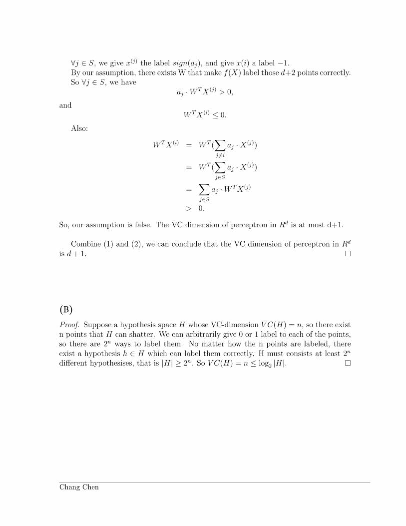
(B)Proof. Suppose a hypothesis space H whose VC-dimension V C(H) = n, so there existn points that H can shatter. We can arbitrarily give 0 or 1 label to each of the points,so there are 2n ways to label them. No matter how the n points are labeled, thereexist a hypothesis h ∈ H which can label them correctly. H must consists at least 2n

different hypothesises, that is |H| ≥ 2n. So V C(H) = n ≤ log2 |H|.

∀j ∈ S, we give x(j) the label sign(aj), and give x(i) a label −1.By our assumption, there exists W that make f(X) label those d+2 points correctly.So ∀j ∈ S, we have

aj ·W TX(j) > 0,

andW TX(i) ≤ 0.

Also: ∑W TX(i) = W T (

j 6=i

aj ·X(j))∑= W T (

j∈S

aj ·X(j))

=∑j∈S

aj ·W TX(j)

> 0.

So, our assumption is false. The VC dimension of perceptron in Rd is at most d+1.

Combine (1) and (2), we can conclude that the VC dimension of perceptron in Rd

is d+ 1.

Chang Chen

(C)Answer: The VC dimension of C is 2.

Proof. First, V Cdim(C) ≤ log2 |C| = log2 10, so V Cdim(C) ≤ 3.Assume there exist X1, X2, X3 ∈ X = {1, 2, ..., 999} that can be shattered by C,

which means all kinds of labels can be realized by concept class C. So ∃{ci1 , ci2 , ..., ci8} ⊂C, which can label X1, X2, X3 as it’s showed in Table 1.

X1 X2 X3

ci1 0 0 0ci2 0 0 1ci3 0 1 0ci4 0 1 1ci5 1 0 0ci6 1 0 1ci7 1 1 0ci8 1 1 1

Table 1

As it can be seen from Table 1, there are at least 3 concepts ∈ C that label X1 tobe 1, so X1 must contains at least 4 different digits. However, X1 ≤ 999, thus it cancontain at most 3 digits.The assumption is proved to be false.

So:V Cdim(C) ≤ 2.

Consider the following Table 2.

34 24c1 0 0c2 0 1c3 1 0c4 1 1

Table 2

As it show in Table 2, 34 and 24 can be shattered by concept class C. So:

V Cdim(C) ≥ 2.

Finally, we can conclude that the VC dimension of C is 2.

Chang Chen

Problem 2

(A)

Proof.Kij = k(xi, xj) = φ(xi) · φ(xj)

cTKc =∑i

∑j

cicjKij

=∑i

∑j

cicjφ(xi) · φ(xj)

= (∑i

ciφ(xi)) · (∑i

ciφ(xi))

= ‖∑i

ciφ(xi)‖22

≥ 0

a)

Proof.

k(x, y) = αk1(x, y) + βk2(x, y)

= 〈√αφ1(x),

√αφ1(y)〉+ 〈

√βφ2(x),

√βφ2(y)〉

= 〈[√αφ1(x),

√βφ2(x)], [

√αφ1(y),

√βφ2(y)]〉

b)

Proof. Let fi(x) be the ith feature value under the feature map φ1, gi(x) be the ith feature valueunder the feature map φ2.

Chang Chen

Then:

k(x, y) = k1(x, y)k2(x, y)

= (φ1(x) · φ1(y))(φ2(x) · φ2(y))

= (∞∑i=0

fi(x)fi(y))(∞∑j=0

gj(x)gj(y))

=∑i,j

fi(x)fi(y)gj(x)gj(y)

=∑i,j

(fi(x)gj(x))(fi(y)gj(y))

= 〈φ3(x), φ3(y)〉

where φ3 has feature hi,j(x) = fi(x)gj(x).

c)Since each polynomial term is a product of kernels with a positive coefficient, the proof followsfrom part a and b.

d)By Taylor expansion:

ex =∞∑i=0

xi

i!

Then the proof follows part c.

(B)

Proof. We wish to show that the kernel k(x,y) = exp(−12‖x − y‖2) can be written as an inner-

product between some mapping φ on x and y, in other words, k(x,y) = 〈φ(x), φ(y)〉. Assumethat x,y ∈ Rd. Consider the formula for φz(x) = (π/2)−d/4 exp(−‖x − z‖2) which is an infinitedimensional function over z ∈ Rd (rather than a finite dimensional vector with z being a discreteindex as we did in class). Similarly, we have φz(y) = (π/2)−d/4 exp(−‖y − z‖2). Then, we definethe kernel as k(x,y) = 〈φz(x), φz(y)〉 =

∫z φz(x)× φz(y)dz. This integral evaluates to

k(x,y) =

∫z(π/2)−d/4 exp

(−‖x− z‖2

)× (π/2)−d/4 exp

(−‖y − z‖2

)dz

= (π/2)−d/2∫z

exp(−x>x− z>z + 2x>z

)exp

(−y>y − z>z + 2y>z

)dz

= (π/2)−d/2 exp(−x>x− y>y

)∫z

exp(−2z>z + 2 (y + x)> z

)dz

Chang Chen

Define r = (y + x)/2 for short-hand and write...

k(x,y) = (π/2)−d/2 exp(−x>x− y>y

)∫z

exp(−2z>z + 4r>z

)dz

= (π/2)−d/2 exp(−x>x− y>y

)exp

(2r>r

)∫z

exp(−2z>z + 4r>z− 2r>r

)dz

= (π/2)−d/2 exp(−x>x− y>y

)exp

(2r>r

)∫z

exp(−2‖z− r‖2

)dz

= (π/2)−d/2 exp(−x>x− y>y

)exp

(2r>r

)(π/2)d/2

= exp(−x>x− y>y

)exp

(1

2x>x +

1

2y>y + x>y

)= exp

(−1

2x>x− 1

2y>y + x>y

)= exp

(−1

2‖x− y‖2

)

Chang Chen

Problem 3

a)

By applying Lagrangian, we can write the primal as:

minξ,w

maxαL(ξ, w, α)

where

L(ξ, w, α) =

n∑i=1

ξ2i + λw>w −n∑i=1

αi(w>xi − yi − ξi),

α ∈ R,

Then we write the dual:maxα

minξ,wL(ξ, w, α)

Take partial derivatives over ξ, w.∂L∂ξi

= 2ξi + αi = 0

∂L∂w

= 2λw −n∑i=1

αixi = 0

Therefore,

ξ = −α2, w =

1

2λXα.

Plug in ξ, w,

LD(α) =1

4α>α+

1

4λα>X>Xα− 1

2λα>X>Xα+ α>y − 1

2α>α

= −1

4α>α− 1

4λα>X>Xα+ α>y

The dual problem is:maxαLD(α)

Take partial derivative over α, we have:

∂LD∂α

= −1

2α− 1

2λX>Xα+ y = 0

The solution to the dual problem:

α = 2λ(X>X + λI)−1y

Chang Chen

b)

Using the results in part a, we have:

w =1

2λXα = X(X>X + λI)−1y

The linear regression can be written as:

y = y>(X>X + λI)−1X>x =n∑i=1

y>(X>X + λI)−1(xi · x)

Replace x with φ(x), and X>X with Gram matrix K, we get:

α = 2λ(K + λI)−1y

Kernel regression:

y =n∑i=1

y>(K + λI)−1k(xi, x).

Chang Chen

Problem 4

First, we normalize the data X, and then randomly split the dataset in to two half for crossvalidation. Then, we train SVM using polynomial kernel and RBF kernel with different parametersand costs. Testing errors are plotted in the following two graphs.

Chang Chen

Figure 1: Testing errors using polynomial kernel with different orders and costs

Figure 2: Testing errors using RBF kernel with different variances and costs

Chang Chen

Machine Learning Problem Set #2

Problem 4

function ques t ion4

% load the da t a s e tload hw2−2015−datase t ;

n = s ize (X, 1 ) ;i d x t r a i n = randsample (n , n / 2 ) ;

% s p l i t the da t a s e ti d x t e s t = s e t d i f f ( 1 : n , i d x t r a i n ) ;

trnX = X( idxt ra in , : ) ;tstX = X( idx t e s t , : ) ;

trnY = Y( idxt ra in , : ) ;tstY = Y( idx t e s t , : ) ;

% c l a s s i f y us ing po lynomia l sd max = 50 ;e r r d = zeros (1 , d max ) ;

global p1 ;for d=1:d max

p1 = d ;

% tra in[ nsv , alpha , b i a s ] = svc ( trnX , trnY , ’ poly ’ , i n f ) ;

% pred i c tpredictedY = svcoutput ( trnX , trnY , tstX , ’ poly ’ , alpha , b i a s ) ;

% compute t e s t e r rore r r d (d) = s v c e r r o r ( trnX , trnY , tstX , tstY , ’ poly ’ , alpha , b i a s ) ;

end

% p l o t er ror vs po lynomia l degreef = f igure ( 1 ) ;c l f ( f ) ;plot ( 1 : d max , e r r d ) ;print ( f , ’−depsc ’ , ’ poly . eps ’ ) ;

Michelle Tadmor - example solution 5

Machine Learning Problem Set #2

% c l a s s i f y us ing r b f ssigmas = . 1 : . 1 : 2 ;e r r s i gma = zeros (1 , numel ( sigmas ) ) ;for s i gma i =1:numel ( sigmas )

p1 = sigmas ( s i gma i ) ;

% tra in[ nsv , alpha , b i a s ] = svc ( trnX , trnY , ’ rb f ’ , i n f ) ;

% pred i c tpredictedY = svcoutput ( trnX , trnY , tstX , ’ rb f ’ , alpha , b i a s ) ;

% compute t e s t e r rore r r s i gma ( s i gma i ) = s v c e r r o r ( trnX , trnY , tstX , tstY , ’ rb f ’ , alpha , b i a s ) ;

end

% p l o t er ror vs po lynomia l degreef = f igure ( 1 ) ;c l f ( f ) ;plot ( sigmas , e r r s i gma ) ;print ( f , ’−depsc ’ , ’ r b f . eps ’ ) ;

Michelle Tadmor - example solution 6