concentrator optical characterization using computer

5105-140

Solar Thermal Power Systems ProjectParabolic Dish Systems Development

\

DOE/JPL-1060-77

Distribution Category UC-62

ASA-CR-174109 NAS,1.26: 1741 09

I '18.5 0 0 0 50h b

Concentrator Optical CharacterizationUsing Computer MathematicalModelling and Point Source Testing

E.W. DennisonS.L. JohnG.F. Trentelman

LIBRARY COpyA~~~ .•

LANGLEY RESEA~CH CENTERLIBRARY, NASA

W,M:"TON, VIt'tGINIA

September 15, 1984

Prepared for

U.S. Department of Energy

Through an Agreement withNational Aeronautics and Space Administration

byJet Propulsion LaboratoryCalifornia Institute of TechnologyPasadena, California

JPL Publication 84-75

5105-140

Solar Thermal Power Systems ProjectParabolic Dish Systems Development

DOE/JPL-1 060-77

Distribution Category UC-62

Concentrator Optical CharacterizationUsing Computer MathematicalModelling and Point Source Testing

E.Wo DennisonSoL. JohnGo F 0 Trentelman

September 15, 1984

Prepared for

u.s. Department of Energy

Through an Agreement withNational Aeronautics and Space Administration

by

Jet Propulsion LaboratoryCalifornia Institute of TechnologyPasadena, California

JPL Publication 84-75

Prepared by the let Propulsion Laboratory, California Institute of Technology,for the U.S. Department of Energy through an agreement with the NationalAeronautics and Space Administration.

The lPL Solar Thermal Power Systems Project is sponsored by the U.S.Department of Energy and is part of the Solar Thermal Program to develop lowcost solar thermal and electric power plants.

This report was prepared as an account of work sponsored by an agency of theUnited States Government. Neither the United States Government nor anyagency thereof, nor any of their employees, makes any warranty, express orimplied, or assumes any legal liability or responsibility for the accuracy, completeness, or usefulness of any information, apparatus, product, or processdisclosed, or represents that its use would not infringe privately owned rights.

Reference herein to any specific commercial product, process, or service by tradename, trademark, manufacturer, or otherwise, does not necessarily constitute orimply its endorsement, recommendation, or favoring by the United StatesGovernment or any agency thereof. The views and opinions of authorsexpressed herein do not necessarily state or reflect those of the United StatesGovernment or any agency thereof.

ABSTRACT

The optical characteristics of a paraboloidal solar concentrator areanalyzed using the intercept factor curve (a format for image data) todescribe the results of a mathematical model and to represent reduced datafrom experimental testing. This procedure makes it possible not only to testan assembled concentrator, but also to evaluate single optical panels or toconduct non-solar tests of an assembled concentrator.

The use of three-dimensional ray tracing computer programs to calculatethe mathematical model is described. These ray tracing programs can includeany type of optical configuration from simple paraboloids to arrays ofspherical facets and can be adapted to microcomputers or larger computers,which can graphically display real-time comparison of calculated and measureddata.

The technique described herein has demonstrated that

(1) It is possible to create a model for predicting concentratoroptical performance from data obtained at various points of theexperimental testing process, and that

(2) The intercept factor curve is a powerful format for opticalperformance representation whether it is derived from themathematical model or from experimental data.

iii

ACKNOWLEDGMENTS

The mathematical modelling described in this report was developed bycoauthors George F. Trentelman and Susan L. John and was funded partly througha U.S. Department of Energy (DOE) summer research fellowship program andsupport from the Northern Michigan University, Marquette, Michigan. George(Fred) Trentelman is a member of the Physics Department at the University;Susan John is currently with GTE-Sylvania in Mountain View, California.

The work described herein was conducted by the Jet PropulsionLaboratory, California Institute of Technology, for the U.S. Department ofEnergy through an agreement with the National Aeronautics and SpaceAdministration (NASA Task RE-152, Amendment 327; DOE/ALO/NASA InteragencyAgreement No. DE-AM04-80AL13137).

1V

D

f

T

X,Y, Z

Vectors

I

N

R

...............I,N,R

x,y,z

Subscripts

m

p

s

x,y,z

NOMENCLATURE

diameter

focal length

distance from the optical ax~s

point coordinates

incident ray from a reflection point to a single point source

surface normal particular to the paraboloidal surface

reflected ray terminating at the receiving plane

unit vectors

unit vectors parallel to the coordinate axes

mirror coordinates relative to the vertex

coordinate of the reflected ray

coordinate of the point source relative to the vertex

components of a unit vector (direction cosine)

v

CONTENTS

I. INTRODUCTION • . • • • • • • • • • • • • • • • • • • • • • • • • • 1-1

I I • COMPUTER MODEL • • • • • • • • • • • • • • • • • • • • • • . • • • 2-1

III. ABERRATIONAL EFFECTS AND IMPERFECT CONCENTRATORS • • • • • • • • • 3-1

IV. RESULTS AND DISCUSSION • • • • • •• 4-1

A.

B.

C.

D.

FULL MIRROR COMPARISONS.

POINT SOURCE TESTING OF INCOMPLETE MIRRORS •

INTERCEPT FACTOR COMPARISONS WITH ONE PARAMETER.

SOLAR EXTRAPOLATION. • • • • • • • • • • • • • •

. • • 4-1

4-3

. • • • 4-5

• 4-6

V. CONCLUS IONS •• • • • • • • • • • • • • • • • • • • • • • • • • • 5-1

REFERENCES •••••••••••••••••••••••••••••• R-I

APPENDIX: DATA TABLES FOR FIGURES IN TEXT••••••••••••••• A-I

Figures

2-1. Vector Analysis for Three-Dimensional Ray Tracing•••••• 2-2

2-2. Computer-Generated Graphic Display of ParaboloidalConcentrator and Reflected Rays ••••••••••••••• 2-5

3-1. Solar Source Intercept Factors for ParaboloidalConcentrator with No Surface Error and for aPerfect Optical System • • • • • • • • • • • • • • • • • • • 3-2

3-2. Randomly Perturbed Surface Normal on ConcentratorSurface. . . . . . . . . . . . . . . . . . . 3-4

4-1. Computed Model and Experimental Intercept Factors for aParaboloidal Concentrator • • •• • • • • • • • • 4-2

4-2. Model and Experimental Intercept Factors for a PartiallyComplete Concentrator ••••••••• ••••••• • 4-4

vii

Figures

4-3.

4-4.

Projected Solar Source Intecept Factors for aParaboloidal Concentrator. •• ••.• • • •

Solar Source Intercept Factors for Concentratorswith Hypothetical Surface Errors • • • • • • • •

viii

4-7

4-8

SECTION I

INTRODUCTION

This report presents an analysis of solar energy concentrators asoptical elements. A substantial amount of experimental and mathematicalanalyses have already been performed on solar concentrators, but theseanalyses have generally considered the concentrator as a subsystem componentof an overall energy production system. For this reason, characteristics ofthe concentrator optics have not been systematically analyzed in a manner thatis independent of the application.

Any discussion of the operation of a solar concentrator requires adefinition of "performance" and a quantitative measure of performance. Thebasic purpose of a solar concentrator is to image (or focus) solar energy froma large entrance aperture into a small receiver aperture where the radiantenergy is converted into thermal energy. The thermal energy is in turnconverted to electrical energy by way of a heat engine. The operatingefficiency of the thermal-to-electrical energy conversion unit is directlyrelated to the receiver temperature. The temperature of the receiverincreases with the mean energy flux density passing into the receiveraperture. The mean energy flux density increases with the image formingquality of the concentrator, i.e., the smaller the image (with respect to thesize of the concentrator entrance aperture), the higher the flux density.Herein, the optical performance of a solar concentrator is defined as "thedegree to which the concentrator can form a high flux density solar image."Because this report covers only optical imaging, surface reflectance andentrance aperture shading are not included in this definition of performancealthough these factors do have a significant effect on the overall operatingperformance of a solar concentrator.

The term "concentration ratio," or the ratio of the concentrator aperturearea to the receiver aperture area, has often been used to define the opticalperformance of a solar concentrator. This definition has the disadvantage ofbeing both incomplete and subject to misinterpretation because there is noprecise definition of the fraction of the focal plane image that passes throughthe receiver aperture. For example, a 13% change in the receiver apertureradius (corresponding to a 30% change in the concentration ratio) would give a1% change in the total input energy.

There are many ways to describe the image forming quality of an opticalsystem. For solar concentrators, a very practical and generally accepteddescription is the focal plane "intercept factor" curve, which is the same asthe standard optical term "encircled energy." These data can be expressed asa table of measured or calculated points that are presented in graphicalform. The curve indicates the fract~on of the total image energy passingthrough an aperture with a radius that is specified by a linear distance fromthe optical axis in the focal plane or by an angle with the vertex at thecenter of the concentrator. The latter parameter is dimensionless; as aconsequence, the results can be applied to any concentrator regardless oflinear dimensions.

1-1

A practical way to measure the image forming characteristics of areflecting panel or an assembled concentrator is use of a fixed point sourceof light. A high intensity spotlight at a distance of 1000 ft is ideal in amoderately dark environment, but good measurements can also be made with ahigh intensity light source at a distance of several focal lengths from theconcentrator vertex. The size of the image from an extended source isdetermined by both the size of the source and the optical imperfections. Inthis case, it is generally difficult, if not impossible, to make aquantitative determination of the optical imperfections. The finalconfirmation of concentrator performance must be made with the sun as asource, but for preliminary testing the sun has the disadvantage of both highlevels of radiant energy and constant motion.

The intercept factor curve can be directly measured with a photometerand a series of circular apertures. For small panels, a Fresnel lens can beused to image the energy passing through the aperture onto the photometer.For large panels, or an assembled concentrator, an imaging photometer can beused to measure the energy falling outside the aperture of a white annulartarget. With a series of water-cooled apertures and a cold-water cavitycalorimeter, the intercept factor curve can be measured when the concentratoris pointing at the sun. The intercept factor data can also be obtained by theuse of a photometer or radiometer that scans the image. Each aperturemeasurement is divided by the total image measurement to obtain the interceptfactor for that aperture. For ray tracing calculations, each point isdetermined by dividing the number of rays that fall within a specified circleby the total number of rays falling on the concentrator.

An intercept factor curve can describe the image from a point source ata finite or infinite distance, or it can describe the image from the sun. Itis also an ideal format for representing both the measured and calculatedimage data. It can be used to directly determine the collection efficiency ofan existing thermal receiver or determine the relationship between receivertemperature and the optimum receiver aperture radius.

Prototype concentrator systems have been built on the basis of overallsystem analyses and subsequently tested under operating conditions. Difficulties arise when total performance does not meet expectations and there isno direct way to systematically isolate the problems. These problems mayresult from any or all of the concentrator components: mirror geometry andsurface properties, mirror mounting and tracking instabilities, receiverconfiguration and location, etc.

Because the optical performance of the concentrator is paramount to thesuccess of the energy conversion, a detailed systematic study was made of theoptics of a prototype concentrator. l This study was based on an interactive

lThe paraboloidal concentrator used in this analysis for experimental testingis the l2-m-diameter Parabolic Dish Concentrator No.1 (PDC-l), which isdescribed in detail in a companion report entitled Development and Testing ofParabolic Dish Concentrator No.1 by E.W. Dennison and T.O. Thostesen, JetPropulsion Laboratory, 5105-143, November 1984.

1-2

development of a mathematical model and experimental testing procedures.The experimental procedures used a point source of light at a finite distanceand were performed under static mirror conditions. Complete and incompletemirrors were incorporated into the testing to determine concentrator characteristics early in the manufacturing process and to evaluate quality controlprocedures.

Previous analyses (Refs. 1 through 4), for example, have incorporatedall of the system components mentioned into a single comprehensive framework,hence making it difficult to isolate specific effects. Moreover, theseanalyses are specific to paraboloidal concentrators. The mathematicalapproach used by these authors emphasizes geometric considerations andutilizes cone optics (an analysis that incorporates the solar disk as anintrinsic part of the computations) as a procedure. This approach is burdenedwith the problems of transcendental equations that are common to manygeometric optical problems. The references cited tend to minimize therequirement for extensive use of computers and their associated expense, andprovide procedures for circumventing direct numerical analyses.

The procedures presented here also rely on computed results. Withcurrent microcomputing technology, an exact and general formulation can beutilized that is neither disproportionately time-consuming nor expensive andcan be made portable enough for use at test site locations. In addition, theprocedures are not limited to paraboloidal configurations or single mirrorsystems. Facetted mirrors, spherical mirrors, and mirrors of special designmay be modelled and analyzed with equal facility.

1-3

SECTION II

COMPUTER MODEL

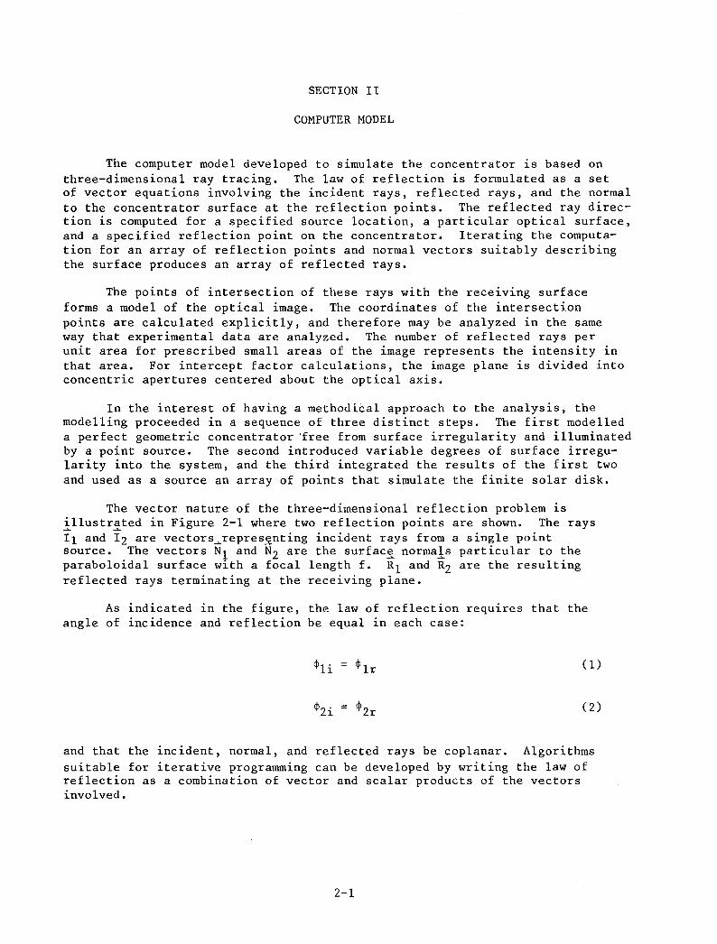
The computer model developed to simulate the concentrator is based onthree-dimensional ray tracing. The law of reflection is formulated as a setof vector equations involving the incident rays, reflected rays, and the normalto the concentrator surface at the reflection points. The reflected ray direction is computed for a specified source location, a particular optical surface,and a specified reflection point on the concentrator. Iterating the computation for an array of reflection points and normal vectors suitably describingthe surface produces an array of reflected rays.

The points of intersection of these rays with the receiving surfaceforms a model of the optical image. The coordinates of the intersectionpoints are calculated explicitly, and therefore may be analyzed in the sameway that experimental data are analyzed. The number of reflected rays perunit area for prescribed small areas of the image represents the intensity inthat area. For intercept factor calculations, the image plane is divided intoconcentric apertures centered about the optical axis.

In the interest of having a methodical approach to the analysis, themodelling proceeded in a sequence of three distinct steps. The first modelleda perfect geometric concentrator 'free from surface irregularity and illuminatedby a point source. The second introduced variable degrees of surface irregularity into the system, and the third integrated the results of the first twoand used as a source an array of points that simulate the finite solar disk.

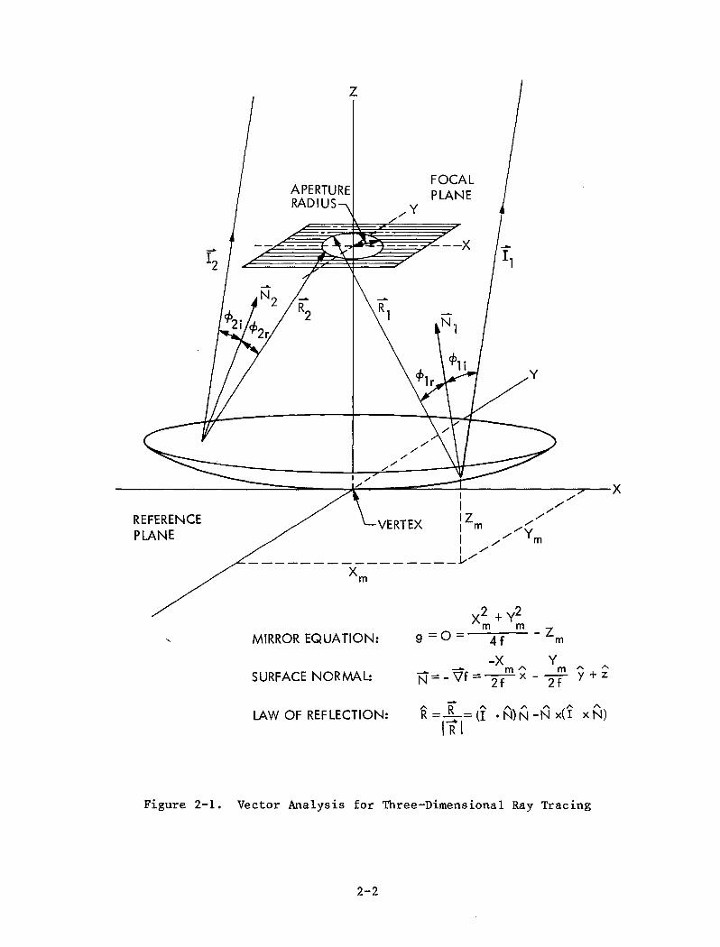
The vector nature of the three-dimensional reflection problem isillustrated in Figure 2-1 where two reflection points are shown. The rays~ ~

11 and 12 are vectors~repres~nting incident rays from a single pointsource. The vectors Nl and N2 are the surfac~ normals particular to theparaboloidal surface with a focal length f. Rl and R2 are the resultingreflected rays terminating at the receiving plane.

As indicated in the figure, the law of reflection requires that theangle of incidence and reflection be equal in each case:

~2i = ~2r

(1)

(2)

and that the incident, normal, and reflected rays be coplanar. Algorithmssuitable for iterative programming can be developed by writing the law ofreflection as a combination of vector and scalar products of the vectorsinvolved.

2-1

REFERENCEPLANE

z

APERTURERADIUS

MIRROR EQUATION:

SURFACE NORMAL:

""Y""

FOCALPLANE

A Ay+Z

LAW OF REFLECTION:A R A A A A A '"

R=-= U •N) N - N x( I x N)IRI

Figure 2-1. Vector Analysis for Three-Dimensional Ray Tracing

2-2

The first step is determining an analytic form for the surface normals.This is accomplished by writing the functional form of the reflecting surfaceas an equipotential surface and taking the negative gradient of the equation.For the paraboloidal surface with the surface equation usually written as:

(3)

(where the subscript m denotes mirror coordinates relative to the vertex and f1S the focal length), the equivalent equipotential is:

o (4)

Application of the negative gradien~ operator

-v (5)

to g(Xm,Ym,Zm) yields the surface normal Nin terms of the coordinatelocation Xm,Ym,Zm of the reflection point as:

N (6)

For a paraboloid this becomes explicitly:

(7)

The latter equation specifies the components of the surface normal vector forany reflection point.

The incident ray vector from any reflection point to the source becomes

I (8)

where Xs ' Ys ' and Zs are the coordinates of the point source relative tothe vertex.

2-3

With this formulation, both the incident ray and the surface normal arenumerically specified. These two vectors are reduced to unit vectors bydividing them by their respective magnitudes:

'"N N/ INI

'"1=1/111.

(9)

(10)

For a point source at infinity, the incident unit vector can also be describedas:

'"I = sino. cos Sx + sin 0. sin Sy + cos 0. Z ( 11)

where 0. is the radial angle from the optical axis and S ~s the azimuthal anglefrom the X axis.

The law of reflection may be written in terms of the scalar (DOT) product(I . N) and the vector (CROSS) product (I x N) to give the associatedreflected ray unit vector as:

'"R (I • N) N N x (I x N) •

This unit vector has three components numerically specified in terms of the x,y, and z directions. These components specify the direction of the reflectedray relative to the coordinate axes.

The vector equation represents three linearly independent componentequations that may be written as a matrix multiplication:

.....R

x

Ry

Rz

(N2 .....2 N2) '" '" ..... '" '"N - 2 N N 2 N N Ix Y z x Y x z x'" '" (N 2 "'2 N2) '" '" '" ( 13)2 N N N - 2 N N I

x Y Y x z Y z Y'" ..... 2 N N (N 2 ..... 2 N2) '"2 N N N I

x z Y z z x y z

As a result, the reflection process is viewed mathematically as a transform ofthe incident ray into the reflected ray with the elements of thetransformation depending only on the surface normal components.

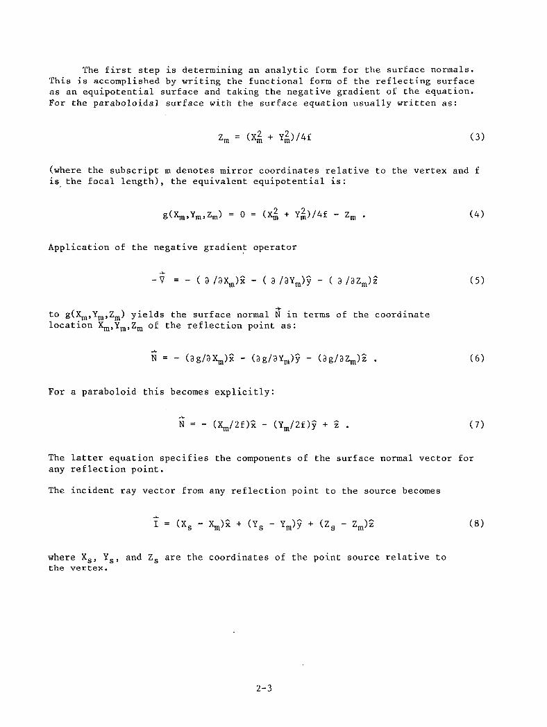
The matrix formulation adapts well to iterative computation, and the useof component multiplication eliminates the need for overt use of trigonometricfunctions. A computer graphic display of the model analogous to Figure 2-1 isshown in Figure 2-2. In the latter figure, the number of zones and the numberof reflection points circumscribing each zone are variable.

2-4

Figure 2-2. Computer-Generated Graphic Display of ParaboloidalConcentrator and Reflected Rays

2-5

The final step in determining the intercept factor is to compute thecoordinates of the reflected ray (designated by the subscript p) as itintercepts the target or focal plane. These coordinates can be found from thegeneral equation:

x - X Y - Y Z - ZP m P m P m .

~ ~ ~

R R Rx Y z

In practice this becomes two equations:

(14)

and

XP

(zp

~

Rx

- Z )*- +m ~

Rz

Xm

(15)

~

RX = (Z - z )*-l + yppm R m

z

The coordinates Xp ' Yp ' and Zp therefore describe an image point whosedistance from the opt~cal axis is:

T= ~,~l\.p ... Ip

(16)

( 17)

and the ray will be inside the aperture if T is less than the radius of theaperture. The intercept factor is the fraction of the total number of raysstriking the concentrator that fall inside the specified focal plane aperture.

2-6

SECTION III

ABERRATIONAL EFFECTS AND IMPERFECT CONCENTRATORS

Because the optical source of primary interest for solar concentratorsis the sun, a practical optical model must include sources of light that areat least one solar radius from the optical axis. The mean half angle of thesolar disk is 4.65 mrad, but for convenience a value of 5 mrad has been usedfor the calculations in this report. For the purpose of the ray tracingmodel, the points on the sun can be either the angular distance from theoptical axis or the X,Y,Z coordinates with respect to the concentratorvertex. (The Z distance of the sun is approximately 1.5 x lOll m.)

For a perfect paraboloid, off-axis source points are not formed intopoint images. These aberrations increase with the angular distance of thepoint source from the optical axis, and the composite effect of theseaberrations is significant. To demonstrate this, an intercept factor curvewas calculated for a paraboloidal concentrator with a focal length/diameter(f/D) of 0.5 and a circular source of 5 mrad radius. The results are shown 1nFigure 3-1, and the data are given in Table 3-1. 2 For comparison, theintercept factor curve for a perfect optical system (no aberrations) with thesame source is also included. The intercept factor is shown as a function ofthe aperture radius divided by the focal length. This dimensionless parameteris the tangent of the aperture radius angle as viewed from the vertex.Because the angles are small and to clarify the interpretation of the curves,the angle is given in milliradians (mrad).

The intercept factor curve for a perfect paraboloid is the upper limitof optical performance. Physical imperfections that extend the interceptfactor must be accounted for in any acceptable model. The model describedhere assumes the uncertainties to be of two categories: systematic and random.

The systematic uncertainties include errors in the geometric form, focallength, and tracking. These errors can be modelled by specifying a differentgeometry for the mirror and by offsetting the solar source from the opticalaxis. However, for the PDC-l concentrator, these errors were detected andcorrected by other direct methods and were eliminated as a major concern inthe final calculations.

Of more relevance to the model is a technique for simulating the randomsurface irregularities that are an inherent part of any concentrator. Becausethe sources of these irregularities are diverse and usually cannot bespecifically isolated, a computational scheme based on random surface errorswas developed and incorporated into the model. The test of such a modellingtechnique is comparison with experimental data.

The model is based on the concept that the surface normals are randomlyperturbed, and these perturbations cause errors in the concentrator image.

2Data tables are given in the Appendix.

3-1

2

0.9

0.8

0.7 -

~

0 0.6I-U«u..I- 0.5a..wU -~wI-Z 0.4

2 - PERFECT OPTICAL SYSTEMSOURCE RADIUS 5 mrad

0.3

0.2

o. 1

--f- t

1 - PERFECT PARABOLOIDAL MIRROR_~ /D -f 0.50, SIGMA 0.00 mrad -

SOURCE RAD IUS 5 mrad ::

=~--

0.0o 2 4 6 8 10 12 14

- f-

16

NORMALIZED APERTURE RADIUS, mrad

Figure 3-1. Solar Source Intercept Factors for ParaboloidalConcentrator with No Surface Error and for aPerfect Optical System

3-2

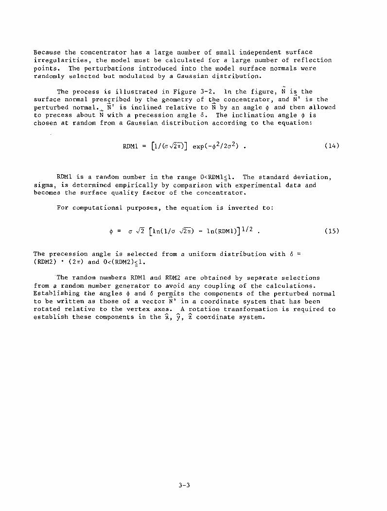
Because the concentrator has a large number of small independent surfaceirregularities, the model must be calculated for a large number of reflectionpoints. The perturbations introduced into the model surface normals wererandomly selected but modulated by a Gaussian distribution.

The process is illustrated in Figure 3-2. In the figure, N i~ thesurface normal prescribed by the geometry of the concentrator, and N' is the..... .....perturbed normal ...... Nt is inclined relative to N by an angle ¢ and then allowedto precess about N with a precession angle o. The inclination angle ¢ ischosen at random from a Gaussian distribution according to the equation:

RDMI (14)

RDMI is a random number in the range O<RDMI~I. The standard deviation,sigma, is determined empirically by comparison with experimental data andbecomes the surface quality factor of the concentrator.

For computational purposes, the equation is inverted to:

a ,J2 [In( l/a J27i) - In(RDMl)] 1/2 •

The precession angle is selected from a uniform distribution with 0 =(RDM2) • (2rr) and O«RDM2)~I.

(15)

"The random numbers RDMI and RDM2 are obtained by separate selectionsfrom a random number generator to avoid any coupling of the calculations.Establishing the angles ¢ and 0 per~its the components of the perturbed normalto be written as those of a vector Nt in a coordinate system that has beenrotated relative to the vertex axes. A rotation transformation is required toestablish these components in the X, y, z coordinate system.

3-3

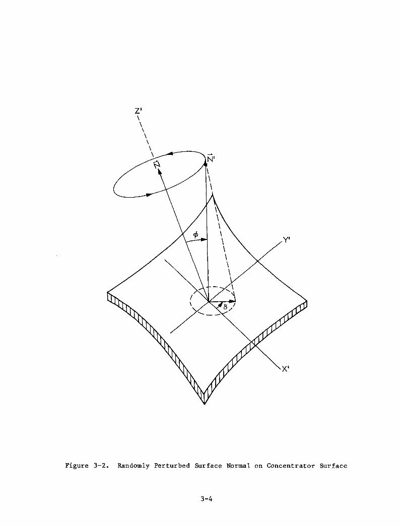
Figure 3-2. Randomly Perturbed Surface Normal on Concentrator Surface

3-4

SECTION IV

RESULTS AND DISCUSSION

As a test of the computer model and of the general procedure,comparisons were made between the model predictions and experimentalmeasurements for a paraboloidal concentrator. This comparison was designedfor three specific objectives: (1) to determine if the modelling procedurehad the credibility and sensitivity required for a practical analytic device,(2) to determine a surface quality factor representative of a specificconcentrator, and (3) to present an accurate extrapolation from the pointsource test data to the solar performance.

The concentrator under study had nominal values of 6.00 m for the focallength and 0.50 for the focal length/diameter ratio (f/D), and for testingpurposes was illuminated with a point source. Experimentally measuredintercept factors were compared with those predicted by the computer model.

The experimental procedures developed for using point sources at finitedistances permitted direct methodical comparison of intercept factors withoutthe necessity of relying on solar models in the analysis. The sun, as afinite source, enlarges the image and obscures the image defects resultingfrom concentrator imperfections. The use of point sources permits an accurateanalysis of the concentrator and allows the experiment to be well defined.The effect of the finite solar source can be calculated after the opticalcharacteristics of the concentrator have been determined.

A. FULL MIRROR COMPARISONS

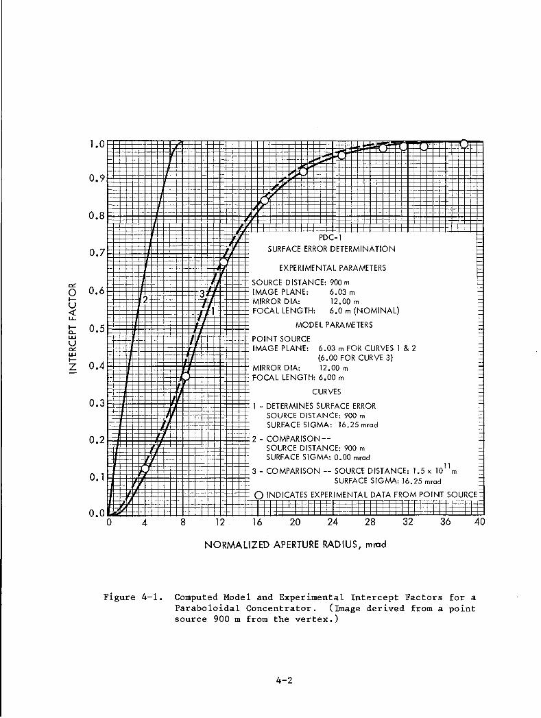
Experimental data for the complete concentrator were gathered with thepoint source (a high quality spotlight) on the optical axis 900 m (nominally150 focal lengths) from the mirror vertex. The image plane was established asthe location of minimum image size and was located 6.03 m from the vertex,very near the nominal focal plane. The intercept factors were determined bymeasuring the amount of light falling on a series of white apertures. Themeasurements were made with an imaging photometer mounted at the concentratorvertex.

The subsequent analysis permitted relatively direct comparison with themodel results. In the ray trace modelling procedures, the intensity isinterpreted as the percentage of rays falling within a circular aperture ~n

the image plane.

The computer model was used in an interactive mode to yield theintercept factor curve shown in Figure 4-1 (data shown in Table 4-1), andestablished a surface error sigma value of 16.25 mrad. Simultaneously, thereal focal length was confirmed to be 6.00 m. The RMS (root mean square)deviation of the curve from the data is approximately 1%. It should be noted,however, that the model curve is not an attempt to fit the data parametrically,

4-1

0.9

0.8

0.7

PDC-I

SURFACE ERROR DETERMINATION

403632282420

-

=~===~:

==-==:

~=SURFACE SIGMA: 16.25 mrad :::

o INDICATES EXPERIMENTAL DATA FROM POINT SOURCE=-r-r-rr--j j --r"-T -,-

16

2 - COMPARISON--SOURCE DISTANCE: 900 mSURFACE SIGMA: 0.00 mrad

3 - COMPARISON -- SOURCE DISTANCE: 1.5 x 101lm

EXPERIMENTAL PARAMETERS

SOURCE DISTANCE: 900 mIMAGE PLANE: 6.03 mMIRROR DIA: 12.00 m

- FOCAL LENGTH: 6.0 m (NOMINAL)

MODEL PARAMETERS

POINT SOURCEIMAGE PLANE: 6.03 m FOR CURVES 1 & 2

(6.00 FOR CURVE 3)MIRROR DIA: 12.00 mFOCAL LENGTH: 6.00 m

CURVES

-- 1 -DETERMINES SURFACE ERRORSOURCE DISTANCE: 900 mSURFACE SIGMA: 16.25 mrad

12

L

3

8

2

4

o. 1

0.3

0.5

0.2

0.0o

0.4

0.6~

oI-u«u..le..u.JU~u.JI-Z


Figure 4-1. Computed Model and Experimental Intercept Factors for aParaboloidal Concentrator. (Image derived from a pointsource 900 m from the vertex.)

4-2

but to establish a surface error number that represents the experimentalintercept factors. The criteria for the best representation was based onsubjective judgment rather than a numeric RMS deviation.

At the beginning of the testing program, there was some concern aboutthe propriety of using a point source at a finite distance because aparaboloidal concentrator gives a well defined image only for an infinitelydistant point source. In practice, this did not present a problem because anaccurate model could simulate any test configuration.

The comparisons between numerous model intercept factors and those forthe experiment did demonstrate that the surface error was the only unknownparameter. For that reason, the nominal values for the focal length, mirrordiameter, image plane distance, and source distance could be used directly inthe final model.

The development of the various computer models necessary to establishthe comparative intercept factors provided valuable information concerning thesensitivity of the model to the physical parameters. In particular, theintercept factor is relatively insensitive to the f/D ratio.

Precise measurement of the experimental image plane position and sourcedistance are crucial to the comparisons, as is a reasonably accurate nominalvalue for the focal length. The most sensitive factor in the modelling is therelative focal point/image plane distance because of the low f/D ratio of theconcentrator. The size of this image changes rapidly with small displacementsof the intercept plane away from the focal point.

Variation of other parameters in addition to the surface error to obtainreasonable model-experiment agreement can be done, but involves looking forsubtle changes in the shape of the intercept factor curve as well as in itsoverall magnitude. For this reason, such comparison depends heavily on theprecision and quantity of experimental data. The excellent agreement of thecomputed data with the experimental data indicated that changes to the nominalparameters were unnecessary.

B. POINT SOURCE TESTING OF INCOMPLETE MIRRORS

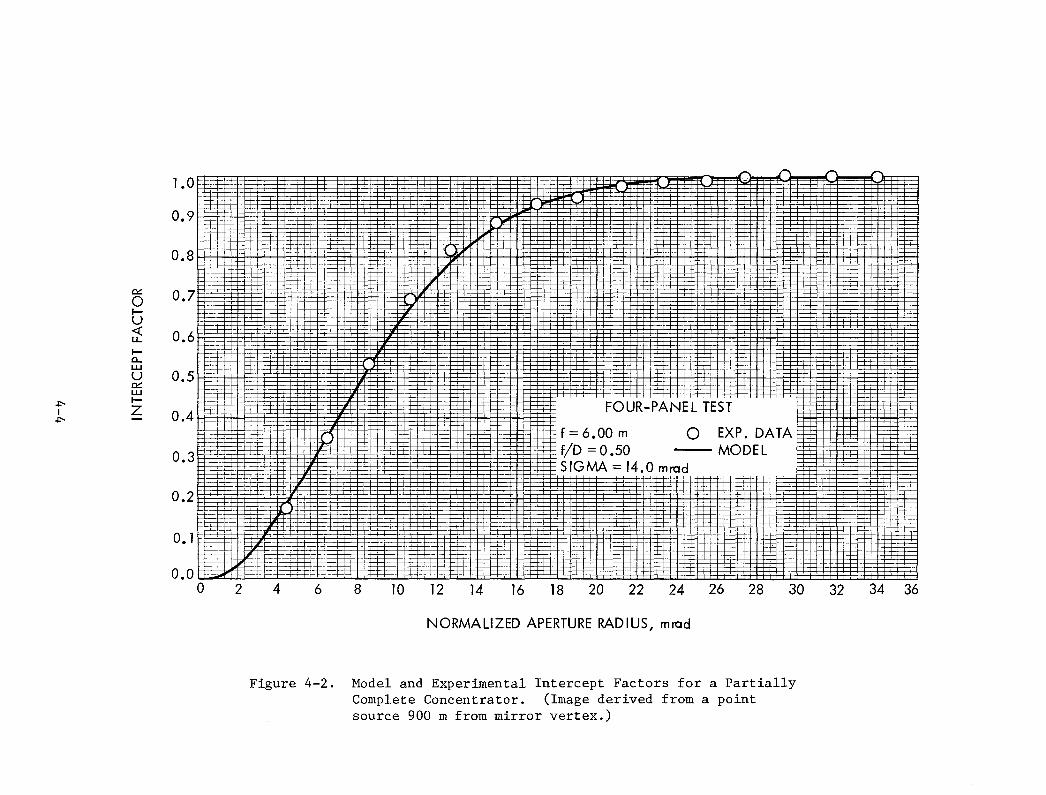
The feasibility of providing mirror quality information during themanufacturing of the concentrator panels was investigated by performing pointsource testing with only four of the twelve panels. The testing procedureswere similar to those used for the complete concentrator, i.e., a point sourceat 900 m was used to illuminate the mirror, and the image was photometricallymeasured to determine the intercept factor.

The experimental and computer model data are shown in Figure 4-2 andTable 4-2. The best comparison for the four-panel system data yielded asurface quality sigma value of 14.0 mrad as the aggregate for the fourpanels. The computer model treated the data as though it were for a completeconcentrator (permissible because of the rotational symmetry) in order todetermine which of the physical parameters required adjustment. Combinations

4-3

,.. '"'"1.0 tel:: -- -- -:=t±-

0.9 t+- :t-

0.8

--'

c::: OJ0I- +U -L« 0.6 + +u.

~

I- -a... r:w L

U 0.50:::w

.p- I-FOUR-PANEL TESTI Z 0.4.p-

-+f 6.00 m 0 EXP. DATA'---+

0.3 ,+ :r 1---' , f/D 0.50 -MODEL-+ _i- -t + SIGMA /4.0 mrad t-

~. --,-,

t-0.2 -+- j-

,.

0.0o

~c::L ++ r'.- -=R=+

2 4 6 8 10 12 14 16 18 20 22 24 26 28 30 32 34 36


Figure 4-2. Model and Experimental Intercept Factors for a PartiallyComplete Concentrator. (Image derived from a pointsource 900 m from mirror vertex.)

of focal length, image plane, diameter, and surface error were modelled. Thestudy provided insight into the sensitivity of the modelling procedures toparametric changes, as well as quantitative data concerning the concentrator.

Two different approaches to the parametric search yielded independent,reasonable representations of the experimental intercept factors. The firstmade the assumption that the effective focal length was 6.0 m, the focallength/diameter ratio was 0.50, and the point source at 900 m was close enoughto infinity to assume imaging at 6.0 m. No acceptable intercept factor wasfound for these parameters. An acceptable intercept factor agreement wasobtained by changing the f/D ratio to 0.54 and by using a surface error sigmaof 12.7 mrad. However, this would imply a mirror diameter of 11.1 m insteadof the actual 12 m. Moreover, modelling a point source at infinity with theseparameters did not give an intercept factor similar to that of the 900-m data.

The second model was constructed to conform as closely as possible tothe actual experimental measurements. The focal length and f/D werereestablished at 6.00 m and 0.50, respectively, but the image plane was set at6.03 m as was actually measured instead of at the previously assumed 6.0 m.These parameters yielded the best comparison and the sigma of 14.0 mrad.These parameters, when modelled for a point source at infinity, give anintercept factor showing the same relationship to the 900-m data as the oneshown in Figure 4-1 for the complete concentrator. This is the relationshipexpected of correct modelling.

These studies of the four-panel assembly reinforce the importance ofaccurately determining the image plane/focal plane distance for point sourcetesting and of accurately measuring the test configuration. This work alsoprovides the basis for further investigation of techniques for analyzingconcentrator optical elements early in their construction.

The difference between the surface quality of the four-panel system andthat of the full mirror is not large, and such an increase in surfaceirregularity is not unexpected as additional panels are installed. Becausethe computer model can be easily tailored to specific parameters and theexperimental measurements can be made within reasonable physical constraints,this modelling method is a promising mode of quality control. Further studyof this application is clearly merited.

C. INTERCEPT FACTOR COMPARISONS WITH ONE PARAMETER

The ability to obtain good model-experiment intercept factor comparisonsusing only one parameter, sigma, as the adjustable parameter should not besurprising because the computation of the surface error actually incorporatestwo variables: (1) the tilt angle of the perturbed normal relative to theideal value and (2) the precession angle of the tilted normal. Bothparameters are called independently from a random number generator. The firstassumes a Gaussian modulation of the random numbers and has a standarddeviation available as an adjustable parameter. The second assumes a uniformdistribution of the precession angles. As a result, the second parameter has

4-5

no standard deviation and does not appear explicitly. The inclusion of thetwo independent parameters does introduce, however, both azimuthal and radialeffects of surface irregularities and, thus, gives a reasonable representationof the actual optical surface.

D. SOLAR EXTRAPOLATION

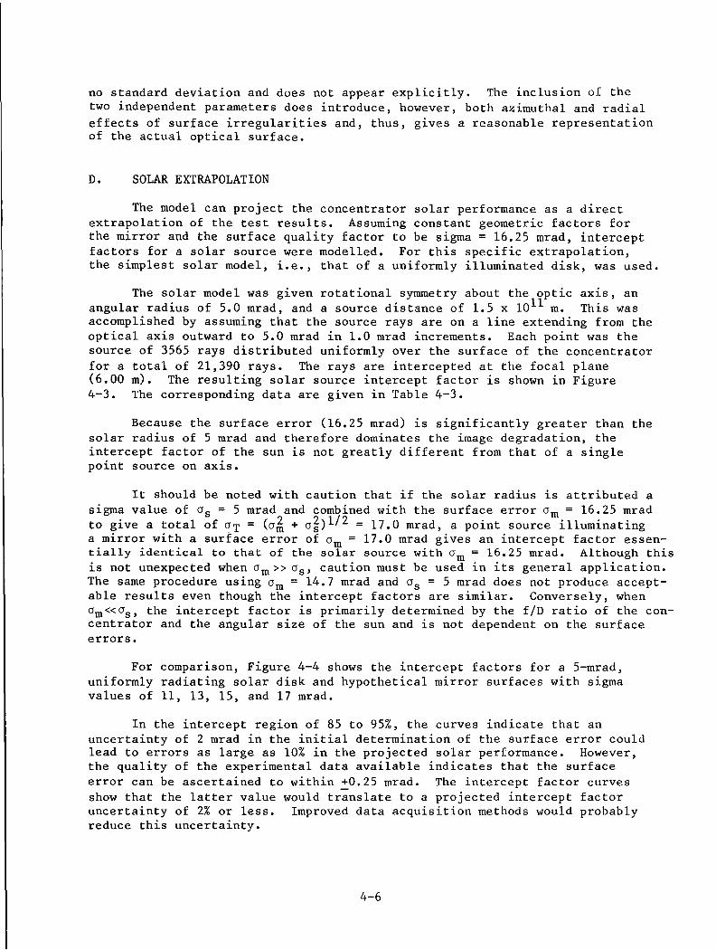
The model can project the concentrator solar performance as a directextrapolation of the test results. Assuming constant geometric factors forthe mirror and the surface quality factor to be sigma = 16.25 mrad, interceptfactors for a solar source were modelled. For this specific extrapolation,the simplest solar model, i.e., that of a uniformly illuminated disk, was used.

The solar model was given rotational symmetry about the optic axis, anangular radius of 5.0 mrad, and a source distance of 1.5 x lOll m. This wasaccomplished by assuming that the source rays are on a line extending from theoptical axis outward to 5.0 mrad in 1.0 mrad increments. Each point was thesource of 3565 rays distributed uniformly over the surface of the concentratorfor a total of 21,390 rays. The rays are intercepted at the focal plane(6.00 m). The resulting solar source intercept factor is shown in Figure4-3. The corresponding data are given in Table 4-3.

Because the surface error (16.25 mrad) is significantly greater than thesolar radius of 5 mrad and therefore dominates the image degradation, theintercept factor of the sun is not greatly different from that of a singlepoint source on axis.

It should be noted with caution that if the solar radius is attributed asigma value of as = 5 mrad and combined with the surface error am = 16.25 mradto give a total of aT = (a~ + a~)1/2 = 17.0 mrad, a point source illuminatinga mirror with a surface error of am = 17.0 mrad gives an intercept factor essentially identical to that of the solar source with am = 16.25 mrad. Although thisis not unexpected when am» as' caution must be used in its general application.The same procedure using am = 14.7 mrad and as = 5 mrad does not produce acceptable results even though the intercept factors are similar. Conversely, whenam«as , the intercept factor is primarily determined by the flD ratio of the concentrator and the angular size of the sun and is not dependent on the surfaceerrors.

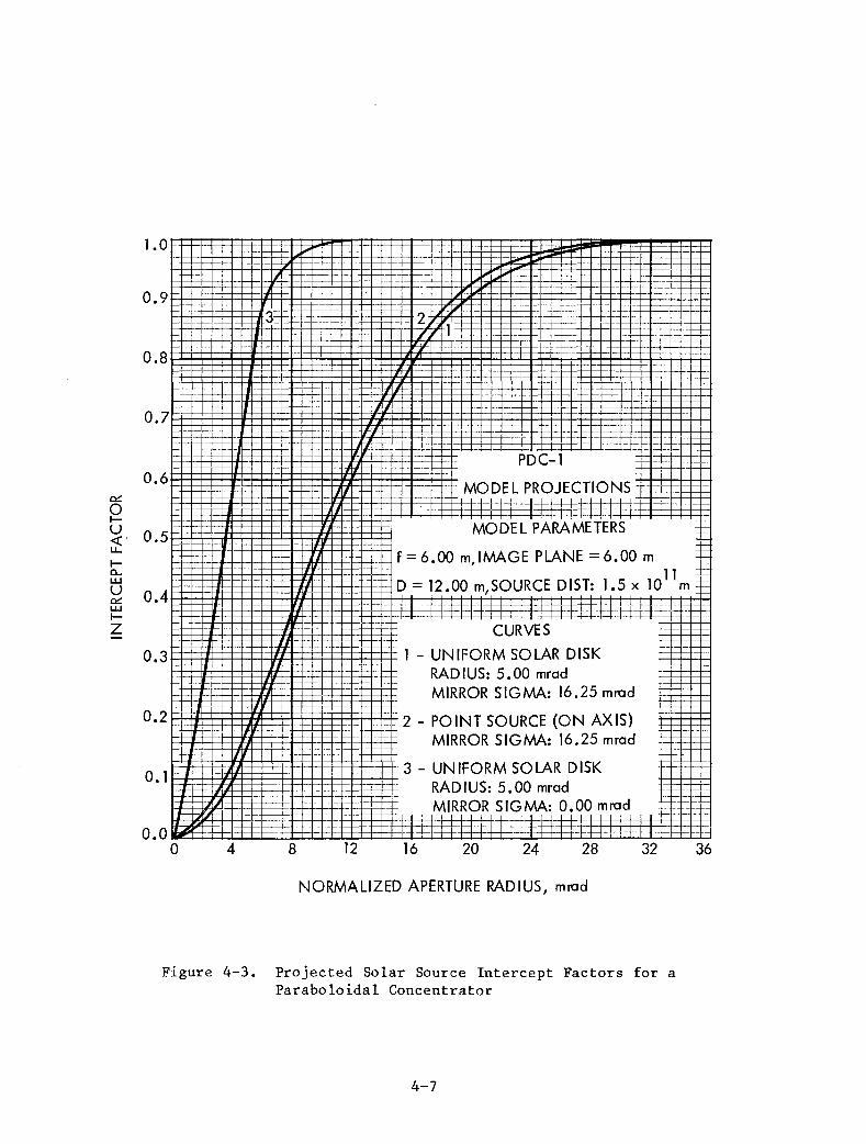
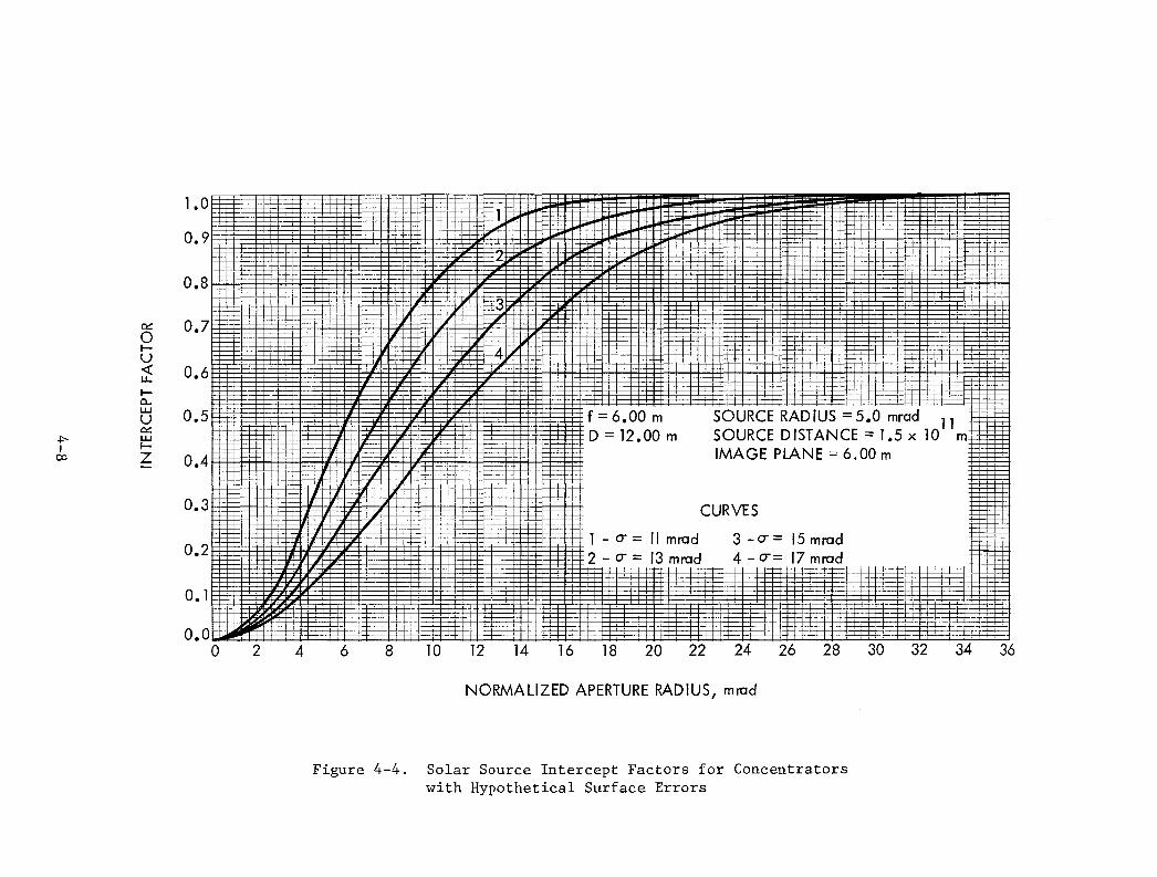
For comparison, Figure 4-4 shows the intercept factors for a 5-mrad,uniformly radiating solar disk and hypothetical mirror surfaces with sigmavalues of 11, 13, 15, and 17 mrad.

In the intercept region of 85 to 95%, the curves indicate that anuncertainty of 2 mrad in the initial determination of the surface error couldlead to errors as large as 10% in the projected solar performance. However,the quality of the experimental data available indicates that the surfaceerror can be ascertained to within ~0.25 mrad. The intercept factor curvesshow that the latter value would translate to a projected intercept factoruncertainty of 2% or less. Improved data acquisition methods would probablyreduce this uncertainty.

4-6

0.9

0.8

t--

3

",

0.4

CURVES

1 - UNIFORM SOLAR DISKRADIUS: 5.00 mrad

. I- MIRROR SIGMA: 16.25 mrad- l-

I- 2 _ POINT SOURCE (ON AXIS)MIRROR SIGMA: 16.25 mrad

. 3 - UNIFORM SOLAR DISK- RADIUS: 5.00 mrad

MIRROR SIGMA: 0.00 mrad

0.7

0.6~

oI-u«, 0.5u..I0WU~wI-Z

0.3

0.2 I

o. 1

.+-

. - f

D

PDC-l ttt~-.--. MODEL PROJECTIONS

~=f~MODEL PARAMETERS

6.00 m,IMAGE PLANE 6.00 m11

12.00 m,SOURCE DIST: 1.5 x 10 m

.+-+-+---i::ttti:f-'=t-··

+-

0.0o 4 8 12 16 20 24 28 32 36


Figure 4-3. Projected Solar Source Intercept Factors for aParaboloidal Concentrator

4-7

18 20 22 24 26 28 30 32 34 36161412108642

1..1..+- -+-

-

-

::j: 2- ,

-r t , +:T+ +-

Lf -- ,-c. .

3c-I--

-- -t

--,.4

""---.--4,

-- f---L

-i-

- f 6.00 m SOURCE RADIUS 5.0 mradD 12.00 m SOURCE DISTANCE 1.5 x 1011 m

IMAGE PLANE 6.00 m-,

tL

-!---

f: CURVES, , ,

1 - a- "mrad 3 -IJ 15 mrad2 -IJ 13 mrad 4 -IJ 17 mrad

+-,- -~ ---' --+-+--

.j:::+ -+--+- -+-- ,"

-t-,--- L+_-,-_L

_---L. ' , '_L.L=F= -+{i,, -+- - q:::p::;:

0.2

0.6

o. 1

0.3

0.4

0.8

0.5

0.0o

1.0

0.9

0.7e:::oIU<{u..I0W

Ue:::wI-

Z~I

00


Figure 4-4. Solar Source Intercept Factors for Concentratorswith Hypothetical Surface Errors

It should be noted that the measurements were made under static mirrorconditions. During actual operation with the concentrator tracking the sun,uncertainties in tracking position and the changing gravity load could affectthe total performance. Measurements of this type can be made with cold-watercalorimeters, but are generally time-consuming and limited to a few aperturevalues.

4-9

SECTION V

CONCLUSIONS

The use of basic paraboloidal geometry with the flD ratio and a singlesurface or slope error as the fundamental parameters to describe a solarconcentrator is cornmon to both this work and that of previous authors. It 1S

reassuring to note that these different approaches give similar results.

The problem with previous solar concentrator models is that they cannotbe used for simple testing of single optical panels or non-solar tests ofassembled concentrators. This problem has been resolved by the use of theintercept factor curve with a point source of light at any distance from theconcentrator or with the sun as a source. The intercept factor curve can beused to describe the results of a mathematical model of a concentrator or torepresent reduced data from experimental image measurements. Measurements canbe made by scanning a photodetector or flux mapper over the image or by theuse of an integrating photometer or calorimeter to measure the relativeintensity of the image falling inside a series of circular apertures. Withthe sun as a source, these intercept factor curves can be used to evaluate theperformance of power conversion thermal receivers.

The use of ray tracing computer programs as described herein is bothpowerful and practical. These programs can include any type of opticalconfiguration from simple paraboloids to arrays of spherical facets. Theseprograms can be adapted to microcomputers at an acceptable cost in operatingtime. The sophisticated graphics displays now available on manymicrocomputing systems can be used for real-time interactive comparison ofcalculated and measured data.

When the optical testing of the JPL PDC-l solar concentrator began,there was a clear need for a comprehensive method to handle both thetheoretical and experimental aspects of imaging characteristics of solarconcentrators. While the work described in this report is not definitive, itdoes demonstrate that the use of ray tracing programs and intercept factorcurves can provide a practical way to fulfill this need.

5-1

REFERENCES

1. Wen, L., Huang, L., Poon, P., and Carley, W., "Comparative Study ofSolar Optics of Paraboloidal Concentrators," ASME, 79-WA/Sol-8, 1979.

2. Wen, L., "Effects of Optical Surface Properties on High TemperatureSolar Thermal Energy Conversion," Journal of Energy, Vol. 3, No.2, 1979.

3. O'Neill, M.J., and Hudson, S.L., "Optical Analysis of Paraboloidal SolarConcentrators," Proceedings of the 1978 SPIE Annual Meeting, Vol. 2,1978, pp. 855-862.

4. Dendt, P., and Rabl, A., "Optical Analysis of Point Focus ParaboloidalRadiation Concentrators," Applied Optics, Vol. 20, 1981, pp. 674-683.

R-l

Model Computed Intercept Factor Data for Figure 3-1. • • • • A-3

Model Computed and Experimental Data for Figure 4-1.. • A-4

Model Computed and Experimental Data for Figure 4-2••••• A-8

Table 3-1.

Table 4-1.

Table 4-2.

Table 4-3.

APPENDIX

DATA TABLES FOR FIGURES IN TEXT

Model Computed Solar Source Projections for Figure 4-3

A-l

• A-10

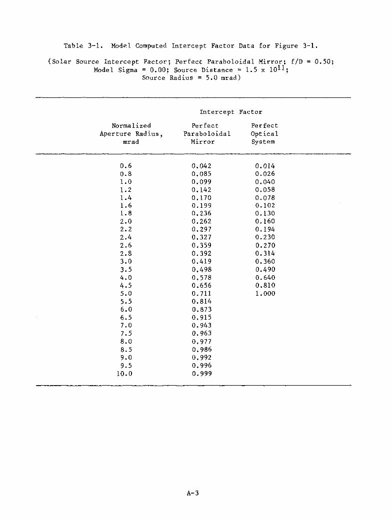
Table 3-1. Model Computed Intercept Factor Data for Figure 3-1.

(Solar Source Intercept Factor; Perfect Paraboloidal Mirror; flD = 0.50;Model Sigma = 0.00; Source Distance = 1.5 x lOll;

Source Radius = 5.0 mrad)

Intercept Factor

NormalizedAperture Radius,

mrad

0.60.81.01.21.41.61.82.02.22.42.62.83.03.54.04.55.05.56.06.57.07.58.08.59.09.5

10.0

PerfectParaboloidal

Mirror

0.0420.0850.0990.1420.1700.1990.2360.2620.2970.3270.3590.3920.4190.4980.5780.6560.7110.8140.8730.9150.9430.9630.9770.9860.9920.9960.999

A-3

PerfectOpticalSystem

0.0140.0260.0400.0580.0780.1020.1300.1600.1940.2300.2700.3140.3600.4900.6400.8101.000

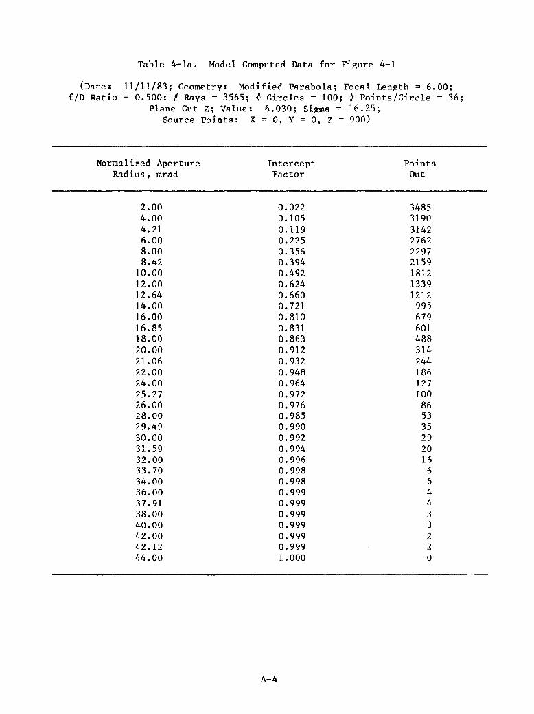
(Date:f/D Ratio

Table 4-1a. Model Computed Data for Figure 4-1

11/11/83; Geometry: Modified Parabola; Focal Length = 6.00;= 0.500; # Rays = 3565; # Circles = 100; # Points/Circle = 36;

Plane Cut z; Value: 6.030; Sigma = 16.25;Source Points: X = 0, Y = 0, Z = 900)

Normalized Aperture Intercept PointsRadius, mrad Factor Out

2.00 0.022 34854.00 0.105 31904.21 0.119 31426.00 0.225 27628.00 0.356 22978.42 0.394 2159

10.00 0.492 181212.00 0.624 133912.64 0.660 121214.00 0.721 99516.00 0.810 67916.85 0.831 60118.00 0.863 48820.00 0.912 31421.06 0.932 24422.00 0.948 18624.00 0.964 12725.27 0.972 10026.00 0.976 8628.00 0.985 5329.49 0.990 3530.00 0.992 2931.59 0.994 2032.00 0.996 1633.70 0.998 634.00 0.998 636.00 0.999 437.91 0.999 438.00 0.999 340.00 0.999 342.00 0.999 242.12 0.999 244.00 1.000 0

A-4

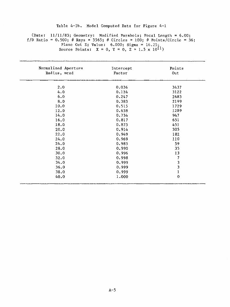
(Date:f/D Ratio

Table 4-lb. Model Computed Data for Figure 4-1


Plane Cut Z; Value: 6.000; Sigma = 16.25i'

Source Points: X = 0, Y = 0, Z = 1.5 x 10 1)


2.0 0.036 34374.0 0.124 31226.0 0.247 26838.0 0.383 2199

10.0 0.515 172912.0 0.638 128914.0 0.734 94716.0 0.817 65118.0 0.873 45120.0 0.914 30522.0 0.949 18224.0 0.969 11026.0 0.983 5928.0 0.990 3530.0 0.996 1332.0 0.998 734.0 0.999 336.0 0.999 338.0 0.999 140.0 1.000 0

A-5

(Date:f/D Ratio

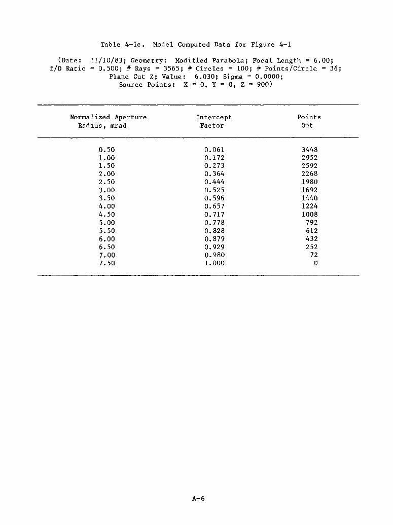
Table 4-1c. Model Computed Data for Figure 4-1




0.50 0.061 3448l.00 0.172 2952l. 50 0.273 25922.00 0.364 22682.50 0.444 19803.00 0.525 16923.50 0.596 14404.00 0.657 12244.50 0.717 10085.00 0.778 7925.50 0.828 6126.00 0.879 4326.50 0.929 2527.00 0.980 727.50 1.000 0

A-6

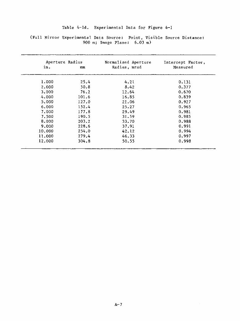
Table 4-1d. Experimental Data for Figure 4-1

(Full Mirror Experimental Data Source: Point, Visible Source Distance:900 m; Image Plane: 6.03 m)

Aperture Radius Normalized Aperture Intercept Factor,in. mm Radius, mrad Measured

1.000 25.4 4.21 0.1312.000 50.8 8.42 0.3773.000 76.2 12.64 0.6704.000 101.6 16.85 0.8395.000 127.0 21.06 0.9276.000 152.4 25.27 0.9657.000 177.8 29.49 0.9817.500 190.5 31.59 0.9858.000 203.2 33.70 0.9889.000 228.6 37.91 0.991

10.000 254.0 42.12 0.99411.000 279.4 46.33 0.99712.000 304.8 50.55 0.998

A-7

(Date:f/D Ratio

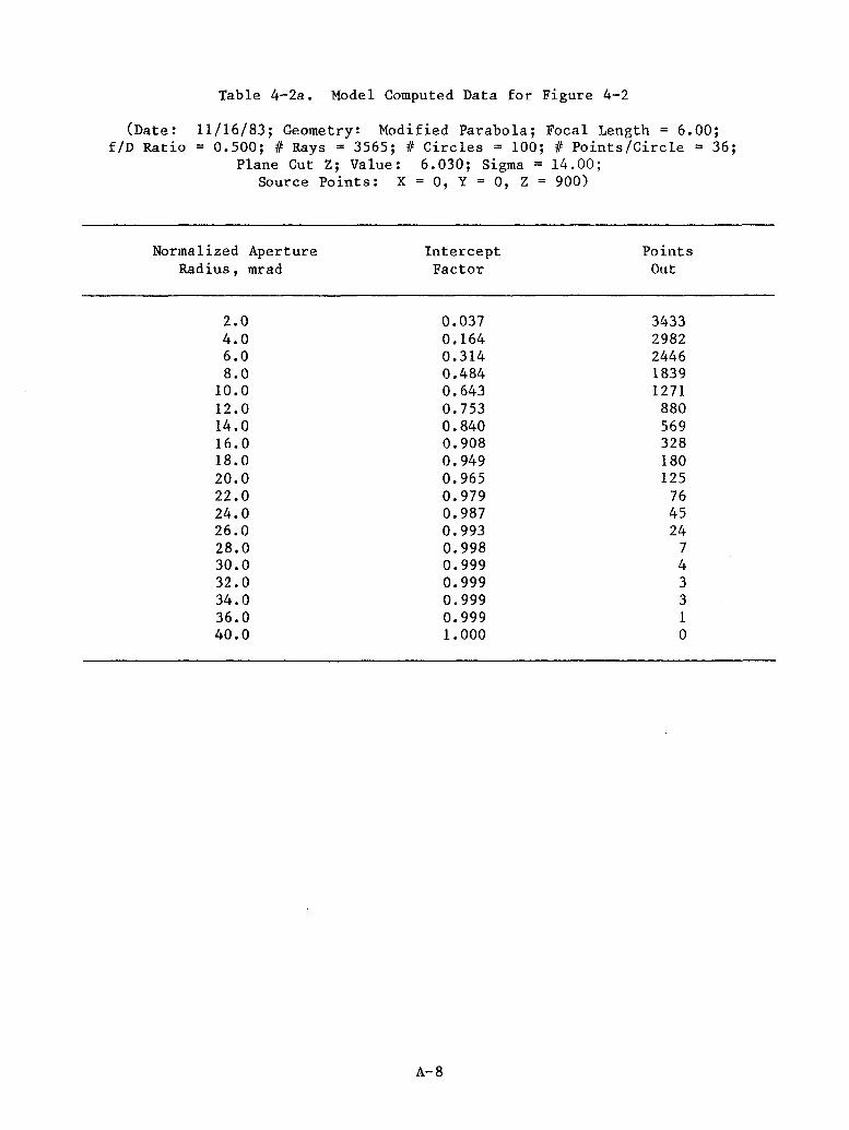
Table 4-2a. Model Computed Data for Figure 4-2

11/16/83; Geometry~ Modified Parabola; Focal Length = 6.00;0.500; # Rays = 3565; # Circles = 100; # Points/Circle = 36;



2.0 0.037 34334.0 0.164 29826.0 0.314 24468.0 0.484 1839

10.0 0.643 127112.0 0.753 88014.0 0.840 56916.0 0.908 32818.0 0.949 18020.0 0.965 12522.0 0.979 7624.0 0.987 4526.0 0.993 2428.0 0.998 730.0 0.999 432.0 0.999 334.0 0.999 336.0 0.999 140.0 1.000 0

A-8

Table 4-2b. Experimental Data for Figure 4-2

(Four Panel Experimental Data Source: Point, Visible Source Distance:900 m; Image Plane: 6.03 m)

Aperture Radius Normalized Aperture Intercept Factor,in. mm Radius, mrad Measured

1.000 25.4 4.23 0.1681.500 38.1 6.35 0.3502.000 50.8 8.47 0.5272.500 63.5 10.58 0.6953.000 76.2 12.70 0.8123.500 88.9 14.82 0.8814.000 101.6 16.93 0.9254.500 114.3 19.05 0.9465.000 127.0 21.17 0.9655.500 139.7 23.28 0.9776.000 152.4 25.40 0.9866.500 165.1 27.52 0.9907.000 177.8 29.63 0.9947.500 190.5 31. 75 0.9978.000 203.2 33.87 0.999

A-9

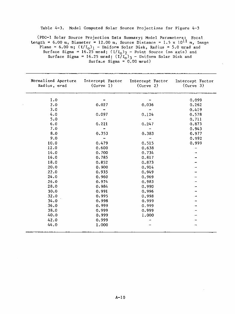
Table 4-3. Model Computed Solar Source Projections for Figure 4-3

(PDC-1 Solar Source Projection Data Summary; Model Parameters: FocalLength = 6.00 m, Diameter = 12.00 m, Source Distance = 1.5 x lOll m, Image

Plane = 6.00 m; (1/10 )1 - Uniform Solar Disk, Radius = 5.0 mrad andSurface Sigma = 16.25 mrad; (1/10 )2 - Point Source (on axis) and

Surface Sigma = 16.25 mrad; (1/10 )3 - Uniform Solar Disk andSurfa~e Sigma = 0.00 mrad)

Normalized ApertureRadius, mrad

Intercept Factor(Curve 1)



1.0 0.0992.0 0.027 0.036 0.2623.0 0.4194.0 0.097 0.124 0.5785.0 0.7116.0 0.221 0.247 0.8737.0 0.9438.0 0.353 0.383 0.9779.0 0.992

10.0 0.479 0.515 0.99912.0 0.600 0.63814.0 0.700 0.73416.0 0.785 0.81718.0 0.852 0.87320.0 0.900 0.91422.0 0.935 0.94924.0 0.960 0.96926.0 0.974 0.98328.0 0.984 0.99030.0 0.991 0.99632.0 0.995 0.99834.0 0.998 0.99936.0 0.999 0.99938.0 0.999 0.99940.0 0.999 1.00042.0 0.99944.0 1.000

A-10

i 1111111111I1111~~IIIIIlIrllllfl]II~11I ~1~1111~ 11111111111, 3 1176 00512 8971

e

concentrator optical characterization using computer

Documents