concept development, floating bridge e39 bjørnafjorden
TRANSCRIPT

Concept development, floating bridge
E39 Bjørnafjorden
Appendix E – Enclosure 7
10205546‐08‐NOT‐098
Bridge closure due to wind

00 24.05.2019 Final issue K. Aas-Jakobsen R. M. Larssen S. E. Jakobsen
REV. DATE DESCRIPTION PREPARED BY CHECKED BY APPROVED BY
MEMO
PROJECT Concept development, floating bridge E39 Bjørnafjorden
DOCUMENT CODE 10205546-08-NOT-098
CLIENT Statens vegvesen ACCESSIBILITY Restricted
SUBJECT Bridge closure due to wind PROJECT MANAGER Svein Erik Jakobsen
TO Statens vegvesen PREPARED BY Ketil Aas-Jakobsen
COPY TO RESPONSIBLE UNIT AMC
SUMMARY
Bridge closure due to wind is discussed for the different bridge alignments in light of the turbulence data in the Metocean Design basis. The discussion shows that bridge closure due to wind may increase due to the increased turbulence intensity from the southern sector. We recommend that this is addressed by an updated analysis. To do these analysis sectorial long term distribution data of the wind is needed (e.g. Weibull parameters).

Concept development, floating bridge E39 Bjørnafjorden
Bridge closure due to wind
10205546-08-NOT-098 24.05.2019 / 00 Page 2 of 4
1 Bridge closure due to wind The Metocean design basis provided in this project indicate that closure due to wind effects on vehicles should be re-evaluated. For certain wind direction the turbulence intensity is specified to 30% /2/ and this will reduce the wind speed for which closure of the bridge must be considered .
N400 states that the structure should be calculated with traffic load up to a 3s gust speed of 35 m/s (N400-§5.4.3.3 /4/). This can be understood as if the gust speed is above 35 m/s, no vehicles is on the bridge, i.e. the bridge is closed. The 3s gust speed can be approximated by U3s = U10min+ 3.5*σu, where σu=Iu*U10min. Thus, by increasing the turbulence intensity, U10min is reduced.E.g. by setting U3s to 35 m/s, the closure wind speed becomes:
A. Iu=11% => U10min = 25.3 m/s
B. Iu=30% => U10min = 17.1 m/s.
The criteria in A above give wind speed similar to closure wind speed used for other bridges worldwide, and similar to the criteria in the previous phase of the Bjørnafjorden crossing. As can be seen in B, if one applies the same method for 30% turbulence intensity, a significantly lower closure speed is found. A reduction of closure speed to this level will increase closure time significantly, and it is questionable if the up-time target for the bridge can be reached without taking measures.
The current Metocean design basis does not contain data about long term distribution, neither for sectorial or omnidirectional data, but by using the results from the calculations in the previous phase the following is found /5/:
U10min is above 25m/s 16 hours yearly
U10min is above 20m/s 69 hours yearly
Thus, a criteria of 17 m/s will give significantly more bridge closing due to wind than the current value of about 16 hours.
In this phase of the project the client has not asked specifically for up-time evaluation of the concepts, as it has not been deemed necessary. Calculations in previous phases has shown that the uptime fulfils the criteria of 99.5%, which corresponds to 43.8 hours of year closure /5/. The above calculation indicates that it will be challenging to reach the 99.5% target without detailed assessment.
In the previous analysis wind in the sector +/- 30 degrees to perpendicular to the vehicles has been viewed as particular important when assessing the effects, as the effective wind attack angle on the vehicle has a significant perpendicular component when one takes into account the speed of the vehicle itself. The critical direction compared to a linearized alignment segment is shown to the right in Figure 1.

Concept development, floating bridge E39 Bjørnafjorden
Bridge closure due to wind
10205546-08-NOT-098 24.05.2019 / 00 Page 3 of 4
Figure 1 Left: Wind rose and area of increased turbulence intensity (Yellow), compared to K12 (Red), K13 (Black) and K14 (Blue).
Right: Critical wind direction compared to alignment (red).
The left part of Figure 1 shows the wind rose with superimposed alignments; K12 (red), K13 (black) and K14 (blue), and the wind direction zone for which elevated turbulence should be applied. Table 1 show a summary of these two figures combined. As can be seen from the table, closure time on Concept K12 and K13 may be affected by the elevated turbulence intensity from the southern sector.
Based on this evaluation we recommend that up-time is re-evaluated for the concepts based on the current Metocean Design Basis. For this sectorial long term distribution is needed, including Weibull parameters.
Table 1 Critical cross wind.
Concept Alignment angle compared to North at
point X in Figure 1 (approx.)
Wind gust direction relative to alignment
Within critical region marked red in Figure 1
K12 + 35o 115o – 175o Yes, partly. Detail assessment
necessary
K13 + 10o 200o – 140o Close. Detail assessment necessary
K14 South: - 5o Mid point: +20o
155o – 215o (South) 130o – 190o (Mid point)
South: No Close. Detail assessment
necessary
X
120
60

Concept development, floating bridge E39 Bjørnafjorden
Bridge closure due to wind
10205546-08-NOT-098 24.05.2019 / 00 Page 4 of 4
2 References
/1/ SBJ-32-C4-SVV-90-BA-001 - Design Basis Bjørnafjorden.
/2/ SBJ-01-C4-SVV-01-BA-001 - Metocean Design Basis.
/3/ NS-EN 1991-1-4:2005+NA:2009. Eurocode 1: Action on structures. Part 1-4: General actions – Wind actions
/4/ N400 Bruprosjektering. Statens Vegvesen.
/5/ Vurdering og sammenlikning av brukonsepter for kryssing av Bjørnafjorden. Oppetid. Versjon 1.0. 25.04.2016.

Concept development, floating bridge
E39 Bjørnafjorden
Appendix E – Enclosure 8
10205546‐08‐NOT‐176
Aerodynamic stability K11

00 24.05.2019 Final issue A. Larsen K. Aas-Jakobsen S. E. Jakobsen
REV. DATE DESCRIPTION PREPARED BY CHECKED BY APPROVED BY
MEMO
PROJECT Concept development, floating bridge E39 Bjørnafjorden
DOCUMENT CODE 10205546-08-NOT-176
CLIENT Statens vegvesen ACCESSIBILITY Restricted
SUBJECT Aerodynamic stability of K11 PROJECT MANAGER Svein Erik Jakobsen
TO Ketil Aas-Jakobsen PREPARED BY Allan Larsen
COPY TO Petter Sundquist RESPONSIBLE UNIT AMC
SUMMARY
This memo summarises the wind stability of the bridge girders of the K11 alternative for Bjørnafjorden bridge. Based on Håndbok N400 the bridge should be aerodynamically stable for speeds up to 81.7m/s.
The memo concludes that the K11 bridge is aerodynamically stable at wind speeds up to and beyond the requirements set by Håndbok N400 Bruprosjektering.

Concept development, floating bridge E39 Bjørnafjorden
Aerodynamic stability of K11
10205546-08-NOT-176 24.05.2019 / 00 Page 2 of 10
1 Wind load class Following N400 /1/, section 5.4.3, a bridge shall be considered wind load class III when the following criteria apply:
Highest eigen period > 2 s
Span length > 300 m
Modal analyses of the K11 alternative for Bjørnafjorden floating bridge yields the highest eigen period to be 126 s. Further the main span of the cable stayed bridge is 380 m.
The above class III criteria are thus seen to be fulfilled. Hence verification of the wind stability of the bridge structure shall include interactions between the dynamics of the structure and wind field as well as aerodynamic stiffness and damping effects. The verification thus includes assessment of vortex induced vibrations /1/ section 5.4.3.7 and check of aerodynamic instabilities /1/ section 5.4.3.8.
2 Critical wind speed for onset of aerodynamic instabilities Following N400 /1/, section 5.4.3 the critical wind speed for onset of aerodynamic instabilities shall be higher than 1.6 times the 500 year return period, 10 min mean wind speed at bridge girder level:
𝑉𝑐𝑟𝑖𝑡(𝑧) > 1.6 ∙ 𝑉𝑚(𝑧, 𝑇 = 600 𝑠, 𝑅 = 500 𝑦𝑒𝑎𝑟) (1)
Following the MetOcean Design Basis /2/ the 50 year return period, 10 min mean wind speed at 𝑧 = 10 m level is 𝑉𝑚(𝑧 = 10 𝑚, 𝑇 = 600 𝑠, 𝑅 = 50 𝑦𝑒𝑎𝑟) = 𝑉𝑚,𝑏 = 30.5 m/s.
Extrapolation to the level of the cable stayed bridge (𝑧 = 65 m) proceeds following (2):
𝑉𝑚(𝑧) = 𝐶𝑝𝑟𝑜𝑏 ∙ 𝑉𝑚,𝑏 ∙ 𝑘𝑇 ∙ 𝑙𝑛 (𝑧
𝑧0) (2)
/2/ defines 𝑘𝑇 = 0.17 and 𝑧0 = 0.01 m for the Bjørnafjord site.
𝐶𝑝𝑟𝑜𝑏 is a coefficient that transforms 50 year return wind speeds to other return periods 𝑅 /3/:
𝐶𝑝𝑟𝑜𝑏 =
√ 1 − 0.2 ∙ 𝑙𝑛 (−𝑙𝑛 (1 −
1𝑅))
1 − 0.2 ∙ 𝑙𝑛 (−𝑙𝑛 (1 −150))
(3)
For 𝑅 = 500 (3) yields 𝐶𝑝𝑟𝑜𝑏 = 1.122. Taking 𝑧 = 65 m, (1), (2) yields 𝑉𝑐𝑟𝑖𝑡(65) > 81.7 m/s.

Concept development, floating bridge E39 Bjørnafjorden
Aerodynamic stability of K11
10205546-08-NOT-176 24.05.2019 / 00 Page 3 of 10
3 Bridge girder aerodynamic properties The present evaluation of the aerodynamic stability of the K11 bridge alternative is based on discrete vortex computations of steady state wind load coefficients and Aerodynamic Derivatives (flutter coefficients) for the SS1-b cross section, Figure 3.1.
The steady state wind load coefficients obtained in /4/ are reproduced in Table 3.1.
Aerodynamic derivatives calculated for the non-dimensional wind speed range 2.5 < 𝑉 𝑓𝐵⁄ < 25 are shown in Figure 3.2
Figure 3.1 Discrete vortex panel model of the SS1-b cross section geometry.
Table 3.1 Steady state wind load coefficients for the SS1-b cross section from discrete vortex simulations.
𝑪𝑫𝟎 [ - ] 𝑪𝑳𝟎 [ - ] 𝒅𝑪𝑳 𝒅𝜶⁄ [𝟏 𝒓𝒂𝒅⁄ ] 𝑪𝑴𝟎 [ - ] 𝒅𝑪𝑴 𝒅𝜶⁄ [𝟏 𝒓𝒂𝒅⁄ ]
0.57 -0.06 3.72 -0.013 0.93*
*𝑑𝐶𝑀 𝑑𝛼⁄ is estimated assuming the aerodynamic centre to be located at the upwind ¼ chord point
The wind load coefficients in Table 3.1 above are normalized the conventional way by the dynamic head of the wind ½𝜌𝑉2 and a characteristic dimension of the cross section. The section depth 𝐻 = 3.5 m in case of the along wind drag loading and the cross section width 𝐵 = 30 m in case of the lift and overturning moment.
Figure 3.2 Aerodynamic derivatives for the SS1-b cross section from discrete vortex simulations.
The aerodynamic derivatives calculated at 6 discrete values of (𝑉 𝑓𝐵⁄ )𝑗, (𝑗 = 1 − 6) shown in
Figure 3.2. The displays the expected behaviour for non-dimensional wind speeds in the range 2.5 < 𝑉 𝑓𝐵⁄ < 18 displaying a monotonic growth in a linear or parabolic fashion. For the highest non-dimensional wind speeds 18 < 𝑉 𝑓𝐵⁄ < 25 it is noted that the 𝐻2..4
∗ and 𝐴2..4∗ aerodynamic
derivatives display an unexpected non-monotonic behaviour which may influence stability calculations slightly.
0 5 10 15 20 2540-
20-
0
20
40
60H1*H2*H3*H4*
V/fB
Ver
tical
0 5 10 15 20 2510-
0
10
20A1*A2*A3*A4*
V/fB
Tors
ion

Concept development, floating bridge E39 Bjørnafjorden
Aerodynamic stability of K11
10205546-08-NOT-176 24.05.2019 / 00 Page 4 of 10
4 Vortex induced vibrations Vortex shedding in the wake of box girders may result in limited amplitude oscillations of the bridge girder at wind speeds where rhythmic vortex shedding locks on to a vertical bending or torsion eigen mode.
Practical experience from suspension bridges with shallow trapezoidal box girders have shown that vortex induced oscillations are usually confined to vertical modes only and occur at low wind speeds typically less than 12 m/s and for weather conditions with low atmospheric conditions.
Vortex induced vibrations of suspension bridges (Osterøy bridge, Norway and Storebælt East bridge, Denmark) has proven to be linked to severe flow separation and associated rhythmic vortex shedding at the knuckle line between the horizontal bottom plate and the lower inclined downwind side panel. Wind tunnel research /5/ has demonstrated that severe flow separation and vortex shedding can be avoided if the angle between the horizontal bottom plate and the lower side panels can be kept at approximately 15 deg. The 15 deg principle was recently introduced for the design of the girder of the Hålogaland Bridge, Norway and has proven to be free of vortex induced vibrations in full scale as well as in wind tunnel tests.
The design of the cross section shape of the girders of Bjørnafjorden bridge incorporates the 15 deg. principle. Thus, vortex induced vibrations are not expected to be an issue for the present design.
Concept development, floating bridge E39 Bjørnafjorden
Aerodynamic stability of K11
10205546-08-NOT-176 24.05.2019 / 00 Page 5 of 10
5 Verification of aerodynamic instabilities N400 specifies that a wind load class III bridge shall be verified for four types of aerodynamic instabilities:
Galloping
Static divergence
Classical flutter
Torsion instability
Each type of aerodynamic instability will be discussed in separate sections below.
Galloping
Galloping is a cross wind vertical instability resulting in onset of vertical divergent oscillations above a certain threshold wind speed.
A necessary condition for galloping to occur is that the lift slope 𝑑𝐶𝐿 𝑑𝛼⁄ is negative. With reference to Table 3.1 𝑑𝐶𝐿 𝑑𝛼⁄ = 3.72 > 0, thus galloping will not occur for the K11 design for Bjørnafjorden bridge.
Static divergence
Static divergence is a buckling type instability of the bridge girder occurring at the wind speed where the wind induced external moment acting on the girder exceeds the structural capacity. An estimate of the wind speed for onset for divergence 𝑉𝑑𝑖𝑣 is given as /1/:
𝑉𝑑𝑖𝑣 = 2𝜋𝑓𝛼√2𝐼𝛼𝑒𝑞
𝜌𝐵4 𝑑𝐶𝑀 𝑑𝛼⁄ (4)
Where:
𝑓𝛼 is the eigenfrequency of the lowest torsion mode having modal mass 𝑀𝛼.
𝐼𝛼𝑒𝑞 =𝑀𝛼
∫ 𝜑(𝑥)2𝑑𝑥𝐿
0
is the corresponding equivalent mass moment of inertia.
𝜌 = 1.25 kg/m³ is air density
𝐵 = over-all girder width
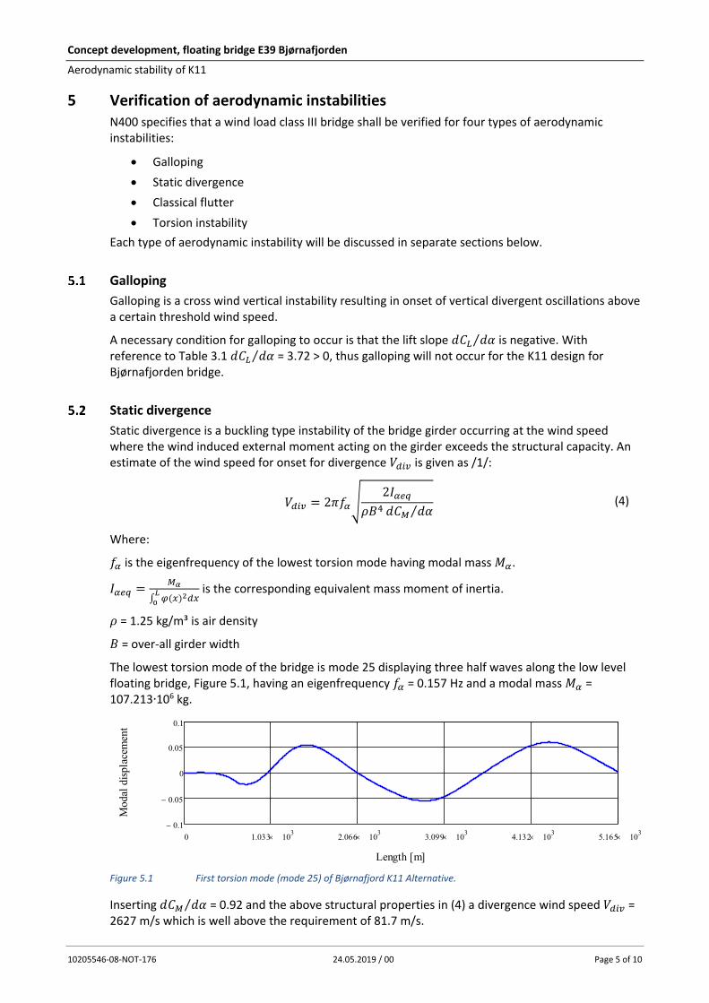
The lowest torsion mode of the bridge is mode 25 displaying three half waves along the low level floating bridge, Figure 5.1, having an eigenfrequency 𝑓𝛼 = 0.157 Hz and a modal mass 𝑀𝛼 = 107.213∙106 kg.
Figure 5.1 First torsion mode (mode 25) of Bjørnafjord K11 Alternative.
Inserting 𝑑𝐶𝑀 𝑑𝛼⁄ = 0.92 and the above structural properties in (4) a divergence wind speed 𝑉𝑑𝑖𝑣 = 2627 m/s which is well above the requirement of 81.7 m/s.
0 1.033 103 2.066 103
3.099 103 4.132 103
5.165 103
0.1-
0.05-
0
0.05
0.1
Length [m]
Mod
al d
ispla
cem
ent

Concept development, floating bridge E39 Bjørnafjorden
Aerodynamic stability of K11
10205546-08-NOT-176 24.05.2019 / 00 Page 6 of 10
Classical flutter
Classical flutter involves as a minimum two modes of motion. A torsion mode and a vertical bending mode of similar mode shape but with a lower eigenfrequency. The critical wind speed for onset of classical flutter is reached when the wind loading on the bridge girder makes the bending and torsion frequencies equal thereby establishing a resonant exchange of energy between to two modes. This in turn leads to divergent coupled torsion bending oscillations of the bridge girder. In cases where more vertical modes exist below the torsion mode these vertical modes may couple to form a compound vertical mode shape which couples with the torsion mode at the onset of flutter.
Different methods exist for calculation of the flutter wind speed of a bridge deck. The present method outlined in section 6 is an expansion of the AMC method (Air material Command) which allows an arbitrary number of modes and degrees of freedom of a bridge deck to couple into flutter /6/. The input to the flutter calculation constitutes the modes assumed to couple into flutter, the corresponding modal masses and eigenfrequencies and aerodynamic derivatives particular to the bridge deck.
The present multi-mode flutter analysis of Bjørnafjorden K11 alternative assumes that the first torsion mode and 9 vertical bending modes may couple into flutter, Figure 5.3. Eigenfrequencies and modal masses with of the modes are listed in Table 5.1.
From the resulting flutter diagrams Figure 5.2 it is noted that all apparent damping levels remain negative for all wind speeds below 120 m/s. Hence the bridge is stable against classical flutter up to and beyond the N400 requirement of 81.7 m/s regardless of structural damping.
Table 5.1 Lowest vertical and torsion modal masses and eigenfrequencies. Bjørnafjord K11 alternative.
Mode 14 Mode 15 Mode 16 Mode 17 Mode 18
Modal mass [kg] 35723∙103 21048∙103 28676∙103 69297∙103 75426∙103
Eigenfrequency [Hz] 0.1596 0.1538 0.1546 01548 0.1548
Mode 19 Mode 20 Mode 21 Mode 22 Mode 25
Modal mass 60315∙103 98445∙103 53534∙103 75942∙103 107213∙103
Eigenfrequency [Hz] 0.1548 0.1548 0.1550 0.1550 0.1567
Figure 5.2 Apparent aerodynamic damping 𝑔 as function of normalized and absolute wind speed for Bjornafjorden K11 alternative.
0 5 10 15 20 250.8-
0.6-
0.4-
0.2-
0
0.2
V/fB
App
aren
t dam
ping
g
0 20 40 60 80 100 1200.8-
0.6-
0.4-
0.2-
0
0.2
Wind speed [m/s]
App
aren
t dam
ping
g

Concept development, floating bridge E39 Bjørnafjorden
Aerodynamic stability of K11
10205546-08-NOT-176 24.05.2019 / 00 Page 7 of 10
Figure 5.3 Flutter modes for Bjørnafjorden bridge K11 alternatives. Modes 14 – 22 (red) are vertical Mode 25 (blue) is torsion.
Mode 14
Mode 15
Mode 16
Mode 17
Mode 18
Mode 19
Mode 20
Mode 21
Mode 22
Mode 25

Concept development, floating bridge E39 Bjørnafjorden
Aerodynamic stability of K11
10205546-08-NOT-176 24.05.2019 / 00 Page 8 of 10
Torsion instability
Torsion instability is a condition resulting in onset of torsional divergent oscillations above a certain threshold wind speed. Torsion instability is associated with the formation and travel of large coherent vortex structures across the bridge deck /6/. This type of instability is often associated with bluff plate girder bridge decks.
A necessary condition for the occurrence of torsion instability is that the 𝐴2∗ aerodynamic derivative
change sign from negative at low wind speeds to positive at higher wind speeds.
From Figure 3.2 it is noted that 𝐴2∗ remains negative for all non-dimensional wind speeds up to at
least 𝑉 𝑓𝐵⁄ = 25. It may thus be concluded that Bjørnafjorden K11 alternative will not encounter torsion instability at wind speeds below a wind speed of 25∙ 𝑓𝛼𝐵 = 117 m/s which is well above the N400 requirement.
6 Multimode flutter theory The calculation of the critical wind speed for onset of flutter follows from solving the complex valued eigenvalue problem (5) which combines the modal and aerodynamic properties of one torsion mode 𝛼(𝑥) and 𝑛 vertical bending modes ℎ1(𝑥)… ℎ𝑛(𝑥), /6/.
𝐷𝑒𝑡
[ 1 + 𝐴𝛼𝛼,𝑗 − 𝜆1,𝑗 ⋯ 𝐴𝛼ℎ𝑛,𝑗
⋮ ⋱ ⋮
𝐻ℎ𝑛𝛼,𝑗 (𝑓𝛼𝑓ℎ𝑛
)2
⋯ (1 + 𝐻ℎ𝑛ℎ𝑛,𝑗) (𝑓𝛼𝑓ℎ𝑛
)2
− 𝜆𝑛,𝑗]
= 0 (5)
The individual elements in (5) combine modal and aerodynamic characteristics of the bridge deck girder and are composed as follows:
𝐴𝛼𝛼,𝑗 =𝜌𝐵4
𝑀𝛼𝐶𝛼𝛼(𝐴3,𝑗
∗ + 𝑖𝐴2,𝑗∗ ), 𝐶𝛼𝛼 = ∫ 𝛼(𝑥)2𝑑𝑥
𝐿
0
𝐴𝛼ℎ𝑛,𝑗 =𝜌𝐵4
𝑀𝛼𝐶𝛼ℎ𝑛(𝐴4,𝑗
∗ + 𝑖𝐴1∗ , 𝑗), 𝐶𝛼ℎ𝑛 = ∫ 𝛼(𝑠)ℎ𝑛(𝑥)𝑑𝑥
𝐿
0
𝐻ℎ𝑛𝛼,𝑗 =𝜌𝐵2
𝑀ℎ𝑛𝐶𝛼ℎ𝑛(𝐻3,𝑗
∗ + 𝑖𝐻2,𝑗∗ ), 𝐶ℎ𝑛𝛼 = ∫ 𝛼(𝑠)ℎ𝑛(𝑥)𝑑𝑥
𝐿
0
𝐻ℎ𝑛ℎ𝑛,𝑗 =𝜌𝐵2
𝑀ℎ𝑛𝐶ℎ𝑛ℎ𝑛(𝐻4.𝑗
∗ + 𝑖𝐻1.𝑗∗ ), 𝐶ℎ𝑛ℎ𝑛 = ∫ ℎ𝑛(𝑥)2𝑑𝑥
𝐿
0
(6)
The unknown to be solved for is the flutter frequency 𝑓 which is embedded in the eigenvalues 𝜆𝑛,𝑗
through the identity:
𝑅𝑒(𝜆𝑛,𝑗) + 𝑖 𝐼𝑚(𝜆𝑛,𝑗) = (1 + 𝑖𝑔𝑛,𝑗) (𝑓𝛼𝑓)2
(7)
Where 𝑔𝑛,𝑗 is the apparent aerodynamic damping (negative) of a given mode at a given non-
dimensional wind speed 𝑉 𝑓𝐵⁄𝑗.
Once the complex eigenvalues 𝜆𝑛,𝑗 are determined for each of the non-dimensional wind speeds
𝑉 𝑓𝐵⁄𝑗= 𝑉𝑗
∗ for which the flutter derivatives are available, the equivalent aerodynamic damping
and corresponding wind speed are obtained as:
𝑔𝑛,𝑗 =𝐼𝑚(𝜆𝑛,𝑗)
𝑅𝑒(𝜆𝑛,𝑗), 𝑉𝑗 = 𝑉𝑗
∗ 𝑓𝛼𝐵
√𝑅𝑒(𝜆𝑛,𝑗) (8)

Concept development, floating bridge E39 Bjørnafjorden
Aerodynamic stability of K11
10205546-08-NOT-176 24.05.2019 / 00 Page 9 of 10
By plotting the equivalent aerodynamic damping 𝑔 as function of the wind speed the critical wind speed is identified where the apparent damping 𝑔𝑛,𝑗 equals twice the structural damping:
𝑔𝑛,𝑗 = 2𝜁 (9)
Example, critical wind speed of Storebælt East Bridge
The above procedure is illustrated in the example below which pairs the aerodynamic derivatives shown in Figure 3.2 with the structural properties of Storebælt East bridge section model (unity modes along the span) for which wind tunnel measurement of the critical wind speeds are reported in the literature /7/.
Storebælt East bridge section model structural data (two modes):
Mass / unit length: 𝑚 = 22.74∙103 kg/m
Mass moment of inertia / unit length: 𝐼 = 2.47∙106 kg/m
Vertical bending frequency: 𝑓ℎ = 0.1 Hz
Torsion frequency: 𝑓𝛼 = 0.278 Hz
Deck width: 𝐵 = 31 m
Structural damping: 𝜁 = 0.003
Determination of the critical wind speed for onset of flutter following the above method is shown in Figure 6.1. It is noted that the red branch remains negative for all wind speeds. The purple branch starts being negative at low wind speeds but intersects the blue horizontal line (twice the structural damping) at a non-dimensional wind speed at 𝑉 𝑓𝐵⁄ = 12.3 (left diagram) corresponding to a critical wind speed of about 79 m/s (right diagram) which may be compared to a critical wind speed in the range 70 – 74 m/s measured in the wind tunnel /7/.
Figure 6.1 Determination of the critical wind speed for onset of flutter in non-dimensional for (left) and actual wind speed (right). Example: Storebælt East Bridge dynamic properties paired with SS1-b aerodynamic dericatives.
The geometry of the Storebælt East bridge and the SS1-b cross section is not identical, thus a perfect match of the above flutter calculation and the Storebælt wind tunnel tests can not be expected. However, the relatively close match is quite satisfactory and supports the credibility of the computed aerodynamic derivatives.
0 5 10 15 20 250.8-
0.6-
0.4-
0.2-
0
0.2
V/fB
App
aren
t dam
ping
g
0 20 40 60 80 1000.8-
0.6-
0.4-
0.2-
0
0.2
Wind speed [m/s]
App
aren
t dam
ping
g

Concept development, floating bridge E39 Bjørnafjorden
Aerodynamic stability of K11
10205546-08-NOT-176 24.05.2019 / 00 Page 10 of 10
7 References /1/ N400: Håndbok, Bruprojektering, Statens vegvesen
/2/ MetOcean Design Basis. Document nr.: SBJ-01-C4-SVV-01-BA-001, 14-11-2018 including addendum of 18-03-2019.
/3/ Eurocode 1: Action on structures – Part 1-4: General actions – Wind actions. 2ed, 2007.
/4/ Memo 10205546-08-NOT-062: CFD analysis of cross section.
/5/ Larsen, A., Wall, A.: Shaping of bridge box girders to avoid vortex shedding response. Journal of Wind Engineering and Industrial Aerodynamics 104-106, (2012) 159-165.
/6/ Larsen, A.: Bridge Deck Flutter Analysis. Proceedings of the Danish Society for Structural Science and Engineering, Vol. 87, No. 2-4, 2016.
/7/ Larsen, A.: Aerodynamic aspects of the final design of the 1624 m suspension bridge across the Great Belt. Journal of Wind Engineering and Industrial Aerodynamics 48, (1993) 261-285.

Concept development, floating bridge
E39 Bjørnafjorden
Appendix E – Enclosure 9
10205546-08-NOT-183
Inhomogeneity in wind – effects on K12
0 15.08.2019 Final issue K. Aas-Jakobsen R. M. Larssen S. E. Jakobsen
REV. DATE DESCRIPTION PREPARED BY CHECKED BY APPROVED BY
INTERNAL - MEMO
PROJECT Concept development, floating bridge E39 Bjørnafjorden
DOCUMENT CODE 10205546-08-NOT-183
CLIENT Statens vegvesen ACCESSIBILITY Restricted
SUBJECT Inhomogeneity in wind – effects on K12 PROJECT MANAGER Svein Erik Jakobsen
TO Statens vegvesen PREPARED BY Ketil Aas-Jakobsen
COPY TO RESPONSIBLE UNIT AMC
SUMMARY
This note shows results from calculation of dynamic transverse response due to wind for concept K12, for four different variations of wind speed along the alignment. Results of variations of the parameters found in Table 15 in the Metocean Design basis is also shown. For the different distributions of the wind speed along the alignment, the case with constant distribution gives the highest dynamic wind response for all directions. Dynamic wind response of xLu, Au, Cux and Cuy is calculated and compared to N400 values. K12 is most sensitive to change in Cuy when the wind is more or less perpendicular to the alignment. For wind in the sector along the alignment the response is less sensitive to change of the calculated parameters.

Concept development, floating bridge E39 Bjørnafjorden
Inhomogeneity in wind – effects on K12
10205546-08-NOT-183 15.08.2019 / 0 Page 2 of 15
Table of Contents 1 Introduction .................................................................................................................................. 3
2 Implementation – calculation of displacement ............................................................................ 4
Calculation of displacement ................................................................................................. 4
Analysis input parameters - wind ......................................................................................... 5
Analysis input parameters – structural ................................................................................. 6
Modes ................................................................................................................................... 7
Load model ........................................................................................................................... 7
3 Verification of calculation method. .............................................................................................. 7
Verification versus hand-calculations ................................................................................... 8
Verification versus Orcaflex .................................................................................................. 9
4 Analysis and Results .................................................................................................................... 11
Introduction ........................................................................................................................ 11
Mean wind variation along the alignment ......................................................................... 11
Variation in Table 15 ........................................................................................................... 12
4.3.1 Introduction ................................................................................................................ 12
4.3.2 Variation of xLu ........................................................................................................... 13
4.3.3 Variation of Au ............................................................................................................ 13
4.3.4 Variation of Cux .......................................................................................................... 14
4.3.5 Variation of Cuy .......................................................................................................... 14
5 Results and Discussion ................................................................................................................ 15
6 References .................................................................................................................................. 15
7 Appendices ................................................................................................................................. 15

Concept development, floating bridge E39 Bjørnafjorden
Inhomogeneity in wind – effects on K12
10205546-08-NOT-183 15.08.2019 / 0 Page 3 of 15
1 Introduction Several floating bridge concepts are proposed for the Bjørnafjorden crossing. This document explore the effect of inhomogeneity in wind the K12 concept, which is the curved bridge with side anchors.
The main focus will be on inhomogeneity effects on dynamic response for K12. K12 is a curved in the horizontal plane and transverse force is carried by the its shape and additional side anchors. The concept is illustrated in Figure 1.
The calculations are done with a simplified, but fast method capable of varying input parameters including wind from all angles and variation of mean wind along the alignment. Results are presented as standard deviations of transverse displacement and strong axis moment. The basic idea is to utilise the eigenmodes of the structure to calculate the response and sum the modal response over all relevant modes. This is a well proven method for calculating dynamic response from wind. However, the simplified method has several disadvantages; currently it has a simplified load model implemented, it does not currently handle geometric stiffness, and damping introduced through the wetted part of the structure is introduced as static modal values for each mode, calculated for the base case with wind perpendicular to the structure. A simplified model is used to adjust the damping for different direction of the wind.
Figure 1 K12 General arrangement.
Concept development, floating bridge E39 Bjørnafjorden
Inhomogeneity in wind – effects on K12
10205546-08-NOT-183 15.08.2019 / 0 Page 4 of 15
2 Implementation – calculation of displacement
Calculation of displacement
Calculation of dynamic response from wind is simplified by including only the resonant part. I.e. the background part is discarded. For lightly damped structures calculations in other projects have shown that this will underestimate the dynamic response with about 5-10%.
The formulation in Eq. 6.50 in /6/ is used for calculating modal response:
𝑄(𝑓𝑒) = 𝜌 ∑ ∑ √(𝐶𝐷𝐻𝑉)𝑖 𝑆𝑢(𝑥𝑖 , 𝑓)(𝐶𝐷𝐻𝑉)𝑗 𝑆𝑢(𝑥𝑗 , 𝑓𝑒)√𝑐𝑜ℎ(𝑓𝑒 , ∆𝑠)𝜑𝑖𝜑𝑗
𝐿
𝑗
𝐿
𝑖
(1)
Where f is the eigenfrequency of the mode and CD, H, V, Su and ϕ is evaluated individually for every element, and √coh is based on the separation of the point and the associated mid-point value.
The standard deviation for the response of each modes is obtained by
𝜎𝑦(𝑓𝑒) = √
𝜋𝑓𝑒4𝜁𝑚
𝑄(𝑓𝑒)
(2𝜋𝑓𝑒)4𝑀𝑚2
(9)
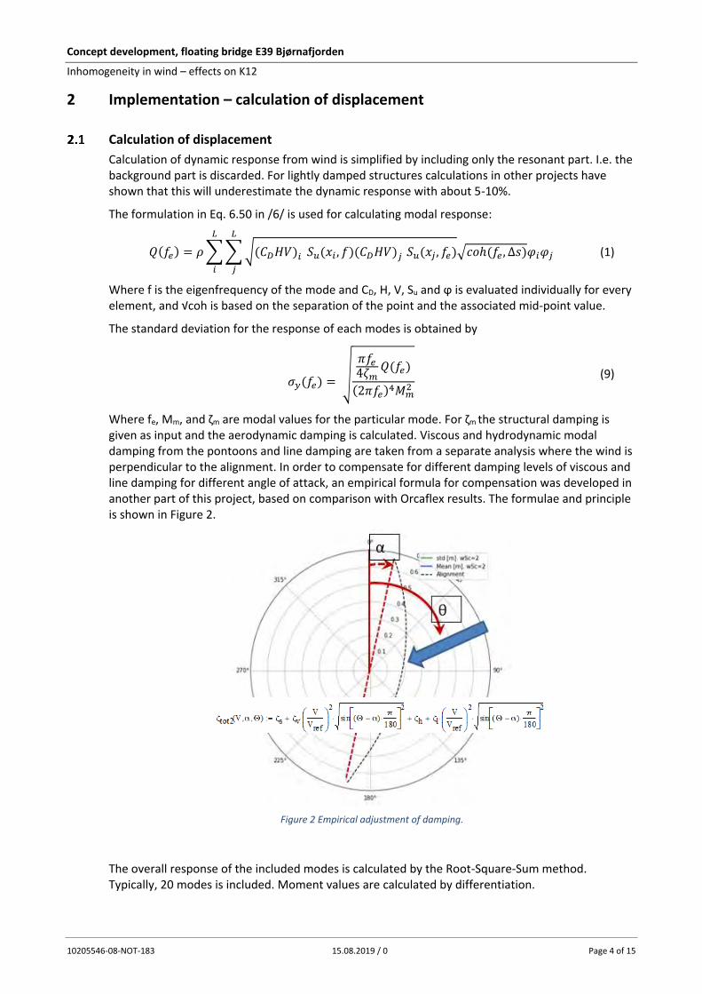
Where fe, Mm, and ζm are modal values for the particular mode. For ζm the structural damping is given as input and the aerodynamic damping is calculated. Viscous and hydrodynamic modal damping from the pontoons and line damping are taken from a separate analysis where the wind is perpendicular to the alignment. In order to compensate for different damping levels of viscous and line damping for different angle of attack, an empirical formula for compensation was developed in another part of this project, based on comparison with Orcaflex results. The formulae and principle is shown in Figure 2.
Figure 2 Empirical adjustment of damping.
The overall response of the included modes is calculated by the Root-Square-Sum method. Typically, 20 modes is included. Moment values are calculated by differentiation.

Concept development, floating bridge E39 Bjørnafjorden
Inhomogeneity in wind – effects on K12
10205546-08-NOT-183 15.08.2019 / 0 Page 5 of 15
Results are presented in a polar diagram similar to the one shown in Figure 3. The angle in this diagram reflects the direction the wind is coming from. 0 degrees is wind from north and 90 degrees is wind from East. A sketch of the alignment is shown as a broken black line.
Figure 3 Principles for response presentation.
Analysis input parameters - wind
The analysis was conducted for wind response only. It was selected to use wind speed with 100year return period and as a first step it was selected to calculate response with the same turbulence intensity for all directions. Thus, standard N400 formulas and values are used in these reference calculations and the wind input to the analysis is:
Basic wind speed at z=10m : vb=25.2m/s Surface roughness: z0=0.01 Length scale at z=10m: xLu=100m Spectral shape parameter: Au=6.8 Decay parameters: Cux=3, Cuy=10, Cuz=10,
Figure 4 Left: Mean wind profile. Right: Spectral distribution with first 20 modes indicated (K12).

Concept development, floating bridge E39 Bjørnafjorden
Inhomogeneity in wind – effects on K12
10205546-08-NOT-183 15.08.2019 / 0 Page 6 of 15
Analysis input parameters – structural
The analysis mode is imported from a master sheet which also is used to build the Orcaflex model. Thus, the geometry is the same as used in the Orcaflex analysis. Modal properties are derived from a NovaFrame analysis with the same structural and geometric properties. This analysis also estimates hydrodynamic, viscous, aerodynamic and line damping for each mode.
Structural damping is generally set to the target value of 0.5% of critical. Since Orcaflex implements damping as Rayleigh damping, it is also implemented in this way in these calculations. The Rayleigh damping for the Orcaflex model is set to the target values for a low and high frequency. Due to the nature of Rayleigh damping the structural damping used in the current calculation is lower than the target value i.e. conservative.
Model used in calculations in this report: K12-06
The simplified load model used in these calculations only take into account the drag loading (See equation (1)). For simplicity CD is extracted for zero angle of attack. The values used for the high and low bridge, Figure 5 and Figure 6, is given in Table 1. In addition drag contributions from columns and cable stays are added at the correct location. Thus, the average Cd of the system is 0.88.
Figure 5 High bridge girder
Figure 6 Low bridge girder
Table 1 Wind load parameters used in calculations.
H [m]
B [m]
CD dCD [1/rad]
CL dCL [1/rad]
CM dCM [1/rad]
High bridge 3.5 30.2 0.67 0.0 0.0 0.0 0.0 0.0
Low Bridge 4.0 30.2 0.80 0.0 0.0 0.0 0.0 0.0
B
H
B
H

Concept development, floating bridge E39 Bjørnafjorden
Inhomogeneity in wind – effects on K12
10205546-08-NOT-183 15.08.2019 / 0 Page 7 of 15
Modes
No of modes used in calculations: 20 (T1=56.8s – T20=6.48s) is shown in Figure 7. Each plot shows transverse modal displacement as red, vertical modal displacement as green and torsional modal rotation as blue. Torsional contribution is scaled up by a factor of 10 to be visible on the plots as can be seen the transverse response dominates the first 14 modes.
Mode 1 – 10 Mode 11-20
Figure 7 Modeplot of first 20 modes of K12_06. Red: Transverse direction, Green: Vertical direction. Blue: torsional component scaled by a factor of 10.
Load model
Currently, only a simplified load in the drag direction is implemented in this method, which only takes into account the fluctuating u-component of the wind. Skew wind is include by a decomposition of the force as shown below. When developing the method further more advanced load models can be implemented. The following load model is used:
FD = 1/2*ρ*(CD* cos(α))*H*U2
3 Verification of calculation method. A flexible python script is developed based on the method described in Section 2.1 and checked versus hand-calculations (Mathcad) and full time-domain simulations in Orcaflex before parameter variations are reported.

Concept development, floating bridge E39 Bjørnafjorden
Inhomogeneity in wind – effects on K12
10205546-08-NOT-183 15.08.2019 / 0 Page 8 of 15
Verification versus hand-calculations
The method described in Section 2.1 is implemented in a Mathcad sheet, see Appendix A. Modal parameters and damping values are imported from Excel sheets. These sheets contain the same modal values as the ones used in the Orcaflex analysis.
The Mathcad sheet only takes into account wind on the girder. Since the Python script also takes into account wind area on cables and columns, an average Cd values is calculated from the Python input and used in Matchad. The weighted average value of the drag coefficients is 0.88 in Python, thus this value is used in the verification.
Mode-by-mode transverse displacement is calculated both in Mathcad and Python and compared for the case with mean wind perpendicular to the main alignment axis. Result comparison of standard deviation of transverse displacement is give in Table 2. As can be seen, the comparison is good both mode-by-mode and RSS over the 5 modes.
Table 2 Comparison of Mathcad and Python script for K12_06. Transverse displacement.
Mode Frequency [Hz]
Total damping [% of crit]
Mathcad – std [m]
Python – std [m]
1 0.018 3.400% 0.930 0.927
2 0.023 3.955% 0.517 0.533
3 0.032 1.988% 0.322 0.315
4 0.046 1.593% 0.145 0.138
5 0.117 4.167% 0.107 0.096
RSS 1.126 1.127
Figure 8 shows a comparison along the alignment between Mathcad and Python, which shows that the agreement is good.
Figure 8 Comparison along alignment. Top: Matchad. Bottom: Python script.

Concept development, floating bridge E39 Bjørnafjorden
Inhomogeneity in wind – effects on K12
10205546-08-NOT-183 15.08.2019 / 0 Page 9 of 15
Verification versus Orcaflex
Verification of the simplified method was done my matching results with Orcaflex for the same input values. Orcaflex calculates the response in the time domain, and are thus, able to include non-linear effects of loading and response. Since Orcaflex has been verified and benchmarked with other calculation codes its reference for this verification.
The simplified method is based on a frequency domain approach, which is significantly faster than the time domain approach used by Orcaflex, but is not capable of handling nonlinearities in e.g. hydrodynamics and aerodynamics, thus, exact match of results are not expected. Results of the comparison are shown in Figure 9. The left figure shows the standard deviation of the displacement, while the right figure shows the calculated strong axis moment. Red dots are Orcaflex values (average of 10 runs), while the blue thick line is results from the simplified method for all wind angles and the doted lines indicate +/- 10% of the simplified method.
Figure 9 Comparison of standard deviation between simplified method and Orcaflex. Blue solid line: Simplified method Blue dotted lines: Simplified method +/- 10%. Red dots: Orcaflex (average of 10 runs). Black broken line: Alignment of K12.
The main purpose of this note is to study the effects and trends of varying wind parameters. Thus, the most important part of the comparison is to see that the simplified model is able to follow the major trends of the Orcaflex calculations.
Displacement results
For wind from east that are close to perpendicular to the alignment good agreement is found on comparison of displacement, while the results deviate more for wind from north and south. For wind from west the displacement shows good agreement. There are some differences in the physics that the models are able to represent that may contribute to the differences.
Possible sources for the deviations are:
- The simplified Python script uses the eigenfrequency only, and thus, discards the background value. Orcaflex uses all load frequencies in response calculations and thus includes the background response. Inclusion of background response will increase the response compared to using only the resonant part. A simplified analysis estimates the background response to about 6% on the standard deviation for the first mode of this structure, see the appendix for calculation.
Mathcad hand calculation

Concept development, floating bridge E39 Bjørnafjorden
Inhomogeneity in wind – effects on K12
10205546-08-NOT-183 15.08.2019 / 0 Page 10 of 15
- Effects of geometric stiffness that slightly changes the vibration frequencies, which again changes how the structure attracts load from the surroundings. This geometric effect is automatically included in Orcaflex, while not included in the modal input in the simplified frequency domain analysis. This is consistent with wind from east increasing the compression in the arc, thus reducing the stiffness, which leads to reduced frequency, and thus, increased response. A simplifed sensitivity study on the above example gave a 7% increase of response for a 3% reduction of vibration frequencies (i.e. softening due to compression in the members).
Strong axis moment
For the strong axis moment the simplified model follows the trend of Orcaflex for all checked wind attack angles. It is noted that larger deviations are found here than for displacement and that the simplified model underestimate the strong axis moment. This is most likely due to a more coarse segmentation of the simplified model, thus not resolving the curvature with the precision needed to get accurate results.
Even though the accuracy of this simplified method is not good enough for design, it is considered good enough for the purpose of this analysis; to look at the effect and differences in response for varying wind.

Concept development, floating bridge E39 Bjørnafjorden
Inhomogeneity in wind – effects on K12
10205546-08-NOT-183 15.08.2019 / 0 Page 11 of 15
4 Analysis and Results
Introduction
The following pages shows maximum transverse displacement as standard deviation for all wind directions for each wind scale types (Root Square Sum values). Results are plotted against the case with uniform wind along the alignment and with standard N400 values. Only wind from the easterly direction is calculated, as the verification calculations (above) showed a fairly symmetric response pattern along the mean alignment.
The following legends is used: Blue solid thick line: Reference value (Results with N400 values) Blue dotted lines: Reference value +/- 10% Black broken line : alignment of the concept. Colored lines: result from parameter variation.
Mean wind variation along the alignment
Figure 10 describes and shows the variation of mean wind along the alignment. The left part of the figure represent the mean wind in the south end of the structure, while the right part of the figure represent the wind in the north end of the structure.
wScaleType Shape
wScaleType=1 wMin=1;wMax=1 Constant=1.0
wScaleType=2 wMin=0.6;wMax=1.0 Linear 0.6->1.0
wScaleType=3; wMin=1.0;wMax=0.6
Linear 1.00->0.6
wScaleType=4; wMin=0.8;wMax=1.0
Bi-linear (mid peak): 0.8->1.0->0.8
Figure 10 Wind variation along the alignment.
A summary of the results is shown in Figure 11. As can be seen the general trend is that constant mean wind (Wind Scale Type 1) gives the highest dynamic response regardless of direction. Second largest effect is from Wind Scale Type 4. Both these cases is symmetric about the mean. The two

Concept development, floating bridge E39 Bjørnafjorden
Inhomogeneity in wind – effects on K12
10205546-08-NOT-183 15.08.2019 / 0 Page 12 of 15
remaining Wind Scale Types are un-symmetric, and the maximum of the two is dependent on the direction of the wind in relation to the structure.
Figure 11 Dynamic response from varying mean wind profile along the deck, see Figure 10. The variation is from south towards north. I.e. for the yellow line the mean wind varies from 0.6 in the south to 1.0 in the north.
Variation in Table 15
4.3.1 Introduction
In Metocean Design basis /2/ Table 15 indicate that parameters in the wind varies. The key parameters are presented as P-values, representing probability of occurrence lower than the specified value. In orderer to understand the effect og the variation several relevant parameters were calculated and compared to the reference value; uniform wind as documented in Section 4.2. Table 3 gives the variations used.
Table 3 Extract from "Table 15". Input varied below marked with blue.*Cux not given in N400. ESDU value is used in reference calculations.
Metocean Design Basis Analysis input (z=10m) (scaled based on N400)
N400 P10 P50 P90 P10 P50 P90
z [m] 10,0 50,0 50,0 50,0 10,0 10,0 10,0
xLu [m] 100,0 108,0 232,0 586,0 66,6 143,2 361,6
xLv [m] 25,0 50,0 141,0 472,0 30,9 87,0 291,2
xLw [m] 8,3 21,0 40,0 81,0 13,0 24,7 50,0
Au 6,8 3,80 7,30 16,30 3,8 7,3 16,3
Av 9,4 5,60 13,30 32,50 5,6 13,3 32,5
Aw 9,4 7,70 12,30 18,20 7,7 12,3 18,2
Cux* 3,0 - - - 5,0 7,0 10,0
Cuy 10,0 6,40 9,00 10,8 6,40 9,00 10,8
Concept development, floating bridge E39 Bjørnafjorden
Inhomogeneity in wind – effects on K12
10205546-08-NOT-183 15.08.2019 / 0 Page 13 of 15
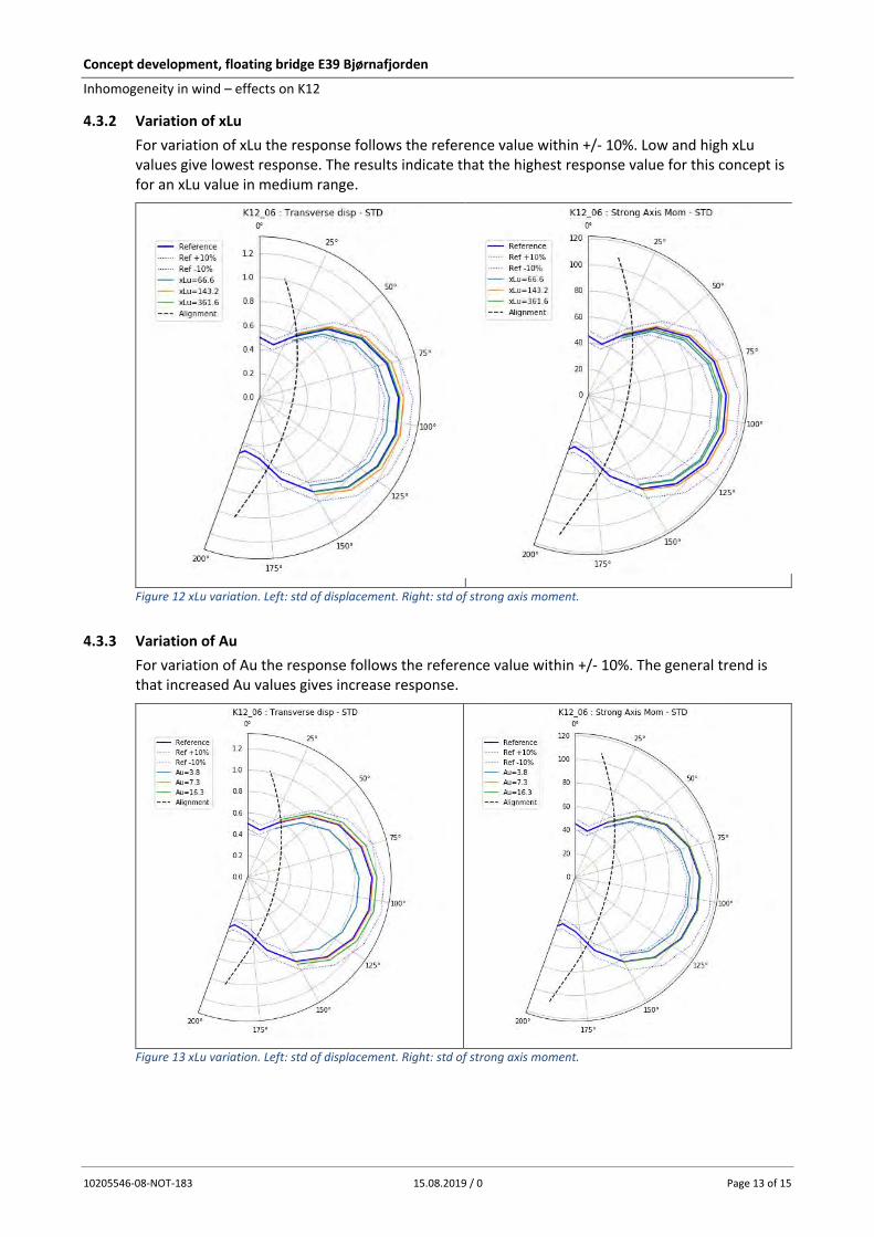
4.3.2 Variation of xLu
For variation of xLu the response follows the reference value within +/- 10%. Low and high xLu values give lowest response. The results indicate that the highest response value for this concept is for an xLu value in medium range.
Figure 12 xLu variation. Left: std of displacement. Right: std of strong axis moment.
4.3.3 Variation of Au
For variation of Au the response follows the reference value within +/- 10%. The general trend is that increased Au values gives increase response.
Figure 13 xLu variation. Left: std of displacement. Right: std of strong axis moment.

Concept development, floating bridge E39 Bjørnafjorden
Inhomogeneity in wind – effects on K12
10205546-08-NOT-183 15.08.2019 / 0 Page 14 of 15
4.3.4 Variation of Cux
For variation of Cux the response follows the reference value within +/- 10%. The effect of change of cux is small for wind perpendicular to the alignment and more pronounced as the wind comes along the alignment. The Cux value of 3.0 used in the reference case gives the highest value of the calculated cases and increase of Cux value give reduced response.
Figure 14 xLu variation. Left: std of displacement. Right: std of strong axis moment.
4.3.5 Variation of Cuy
The calculation of variations of Cuy is shown in Figure 15. As can be seen the response is sensitive to change of Cuy, particularly for wind perpendicular to the alignment. Lower value of Cuy gives higher response and Cuy values below the P10 value of 6.4 increases the response with more than 20%. For skew wind, where the wind is more along the alignment, the effect is less pronounced.
Figure 15 Cuy variation. Left: std of displacement. Right: std of strong axis moment.

Concept development, floating bridge E39 Bjørnafjorden
Inhomogeneity in wind – effects on K12
10205546-08-NOT-183 15.08.2019 / 0 Page 15 of 15
5 Results and Discussion Wind response of K12 for N400 standard wind values is calculated with a simplified method. The model is extracted from Orcaflex and contain the same modal parameters and damping, including hydrodynamic effects. The simplified method is compared to hand calculations and Orcaflex and shows fairly good agreement.
For the different distribution of the wind speed along the alignment, the case with constant distribution gives the highest dynamic wind response for all directions.
Sensitivity within the P10-P90 values is compared to the values given in N400. Of the studied parameters, xLu, Au, Cux and Cuy, Cuy gives the largest difference compare to N400.
For wind more or less perpendicular to the alignment Cuy gives the largest changes compared to N400 values. For wind along the alignment the sensitive to change is larges for Cux, but small in general.
6 References /1/ SBJ-32-C4-SVV-90-BA-001 - Design Basis Bjørnafjorden.
/2/ SBJ-01-C4-SVV-01-BA-001 - Metocean Design Basis.
/3/ NS-EN 1991-1-4:2005+NA:2009. Eurocode 1: Action on structures. Part 1-4: General actions – Wind actions
/4/ N400 Bruprosjektering. Statens Vegvesen.
/5/ Vurdering og sammenlikning av brukonsepter for kryssing av Bjørnafjorden. Oppetid. Versjon 1.0. 25.04.2016.
/6/ Theory of Bridge Aerodynamics. E.Strømmen. Springer. 2006.
7 Appendices Mathcad sheet – Simplified dynamic wind calculation model
Mathcad Sheet – Full dynamic wind calculation model.

Concept development, floating bridge
E39 Bjørnafjorden
Appendix E – Enclosure 10
10205546-08-NOT-184
Aerodynamic stability of K12

0 15.08.2019 Final issue A. Larsen R. M. Larssen S. E. Jakobsen
REV. DATE DESCRIPTION PREPARED BY CHECKED BY APPROVED BY
MEMO
PROJECT Concept development, floating bridge E39 Bjørnafjorden
DOCUMENT CODE 10205546-08-NOT-184
CLIENT Statens vegvesen ACCESSIBILITY Restricted
SUBJECT Aerodynamic stability of K12 PROJECT MANAGER Svein Erik Jakobsen
TO Statens vegvesen PREPARED BY Allan Larsen
COPY TO RESPONSIBLE UNIT AMC
SUMMARY
This memo summarises the wind stability of the bridge girders of the K12 alternative for Bjørnafjorden bridge.
The memo concludes that the bridge is aerodynamically stable at wind speeds up to and beyond the requirements set by Håndbok N400 Bruprosjektering.

Concept development, floating bridge E39 Bjørnafjorden
Aerodynamic stability of K12
10205546-08-NOT-184 15.08.2019 / 0 Page 2 of 11
Table of Contents 1 Wind load class .......................................................................................................................... 3
2 Critical wind speed for onset of aerodynamic instabilities ......................................................... 3
3 Bridge girder aerodynamic properties ........................................................................................ 3
4 Vortex induced vibrations .......................................................................................................... 4
5 Verification of aerodynamic instabilities .................................................................................... 5
Galloping ............................................................................................................................ 5
Static divergence ................................................................................................................ 5
Classical flutter ................................................................................................................... 6
Torsion instability ............................................................................................................... 8
6 Multimode flutter calculation .................................................................................................... 9
Flutter calculation, Storebælt East bridge ........................................................................ 10
7 References ............................................................................................................................... 11

Concept development, floating bridge E39 Bjørnafjorden
Aerodynamic stability of K12
10205546-08-NOT-184 15.08.2019 / 0 Page 3 of 11
1 Wind load class Following N400 /1/, section 5.4.3, a bridge shall be considered wind load class III when the following criteria apply:
Highest eigen period > 2 s
Span length > 300 m
Modal analyses of the K12 alternative for Bjørnafjorden floating bridge yields the highest eigen period to be 56.8 s. Further the main span of the cable stayed bridge is 380 m.
The above class III criteria are thus seen to be fulfilled. Hence verification of the wind stability of the bridge structure shall include interactions between the dynamics of the structure and wind field as well as aerodynamic stiffness and damping effects. The verification thus includes assessment of vortex induced vibrations /1/ section 5.4.3.7 and check of aerodynamic instabilities /1/ section 5.4.3.8.
2 Critical wind speed for onset of aerodynamic instabilities Following N400 /1/, section 5.4.3 the critical wind speed for onset of aerodynamic instabilities shall be higher than 1.6 times the 500 year return period, 10 min mean wind speed at bridge girder level:
𝑉𝑐𝑟𝑖𝑡(𝑧) > 1.6 ∙ 𝑉𝑚(𝑧, 𝑇 = 600 𝑠, 𝑅 = 500 𝑦𝑒𝑎𝑟) (1)
Following the MetOcean Design Basis /2/ the 50 year return period, 10 min mean wind speed at 𝑧 = 10 m level is 𝑉𝑚(𝑧 = 10 𝑚, 𝑇 = 600 𝑠, 𝑅 = 50 𝑦𝑒𝑎𝑟) = 𝑉𝑚,𝑏 = 30.5 m/s.
Extrapolation to the level of the cable stayed bridge (𝑧 = 65 m) proceeds following (2):
𝑉𝑚(𝑧) = 𝐶𝑝𝑟𝑜𝑏 ∙ 𝑉𝑚,𝑏 ∙ 𝑘𝑇 ∙ 𝑙𝑛 (𝑧
𝑧0) (2)
/2/ defines 𝑘𝑇 = 0.17 and 𝑧0 = 0.01 m for the Bjørnafjord site.
𝐶𝑝𝑟𝑜𝑏 is a coefficient that transform 50 year return wind speeds to other return periods 𝑅 /3/:
𝐶𝑝𝑟𝑜𝑏 =
√ 1 − 0.2 ∙ 𝑙𝑛 (−𝑙𝑛 (1 −
1𝑅))
1 − 0.2 ∙ 𝑙𝑛 (−𝑙𝑛 (1 −150))
(3)
For 𝑅 = 500 (3) yields 𝐶𝑝𝑟𝑜𝑏 = 1.122. Taking 𝑧 = 65 m, (1), (2) yields 𝑉𝑐𝑟𝑖𝑡(65) > 81.7 m/s.
3 Bridge girder aerodynamic properties The present evaluation of the aerodynamic stability of the K12 bridge alternative is based on discrete vortex computations of steady state wind load coefficients and Aerodynamic Derivatives (flutter coefficients) for the K12 cross section, Figure 3.1.
The steady state wind load coefficients obtained in /4/ are reproduced in Table 3.1.
Aerodynamic derivatives calculated for the non-dimensional wind speed range 4 < 𝑉 𝑓𝐵⁄ < 30 are shown in Figure 3.2

Concept development, floating bridge E39 Bjørnafjorden
Aerodynamic stability of K12
10205546-08-NOT-184 15.08.2019 / 0 Page 4 of 11
Figure 3.1 Discrete vortex panel model of the K12 cross section geometry.
Table 3.1 Steady state wind load coefficients for the K12 cross section from discrete vortex simulations.
𝐶𝐷0 [ - ] 𝐶𝐿0 [ - ] 𝑑𝐶𝐿 𝑑𝛼⁄ [1 𝑟𝑎𝑑⁄ ] 𝐶𝑀0 [ - ] 𝑑𝐶𝑀 𝑑𝛼⁄ [1 𝑟𝑎𝑑⁄ ]
0.675 -0.413 3.122 0.012 0.916
The wind load coefficients in Table 3.1 above are normalized the conventional way by the dynamic head of the wind ½𝜌𝑉2 and a characteristic dimension of the cross section. The section depth 𝐻 = 4.0 m in case of the along wind drag loading and the cross section width 𝐵 = 30.2 m in case of the lift and overturning moment.
Figure 3.2 Aerodynamic derivatives for the K12 cross section from discrete vortex simulations.
The simulated aerodynamic derivatives shown in Figure 3.2 display the expected behaviour for non-dimensional wind speeds in the range 4 < 𝑉 𝑓𝐵⁄ < 18 displaying a monotonic growth in a linear or parabolic fashion. For the highest non-dimensional wind speeds 18 < 𝑉 𝑓𝐵⁄ < 30 it is noted that the 𝐻2.4∗ and 𝐴2.4
∗ aerodynamic derivatives displays an unexpected non-monotonic behaviour which may influence stability calculations slightly.
4 Vortex induced vibrations Vortex shedding in the wake of box girders may result in limited amplitude oscillations of the bridge girder at wind speeds where rhythmic vortex shedding locks on to a vertical bending or torsion eigen mode.
0 6 12 18 24 3040-
20-
0
20
40
60H1*H2*H3*H4*
V/fB
Ver
tical
0 6 12 18 24 3010-
0
10
20A1*A2*A3*A4*
V/fB
Tors
ion

Concept development, floating bridge E39 Bjørnafjorden
Aerodynamic stability of K12
10205546-08-NOT-184 15.08.2019 / 0 Page 5 of 11
Practical experience from suspension bridges with shallow trapezoidal box girders have shown that vortex induced oscillations are usually confined to vertical modes only and occur at low wind speeds typically less than 12 m/s and for weather conditions with low atmospheric conditions.
Vortex induced vibrations of suspension bridges (Osterøy bridge, Norway and Storebælt East bridge, Denmark) has proven to be linked to severe flow separation and associated rhythmic vortex shedding at the knuckle line between the horizontal bottom plate and the lower inclined downwind side panel. Wind tunnel research /5/ has demonstrated that severe flow separation and vortex shedding can be avoided if the angle between the horizontal bottom plate and the lower side panels can be kept at approximately 15 deg. The 15 deg principle was recently introduced for the design of the girder of the Hålogaland Bridge, Norway and has proven to be free of vortex induced vibrations in full scale as well as in wind tunnel tests.
The design of the cross section shape of the girders of Bjørnafjorden bridge incorporates the 15 deg. principle. Thus, vortex induced vibrations are not expected to be an issue for the present design.
5 Verification of aerodynamic instabilities N400 specifies that a wind load class III bridge shall be verified for four types of aerodynamic instabilities:
Galloping
Static divergence
Classical flutter
Torsion instability
Each type of aerodynamic instability will be discussed in separate sections below.
Galloping
Galloping is a cross wind vertical instability resulting in onset of vertical divergent oscillations above a certain threshold wind speed.
A necessary condition for galloping to occur is that the lift slope 𝑑𝐶𝐿 𝑑𝛼⁄ is negative. With reference to Table 3.1 𝑑𝐶𝐿 𝑑𝛼⁄ = 3.122 > 0, thus galloping will not occur for the K12 design for Bjørnafjorden bridge.
Static divergence
Static divergence is a buckling type instability of the bridge girder occurring at the wind speed where the wind induced external moment acting on the girder exceeds the structural capacity. An estimate of the wind speed for onset for divergence 𝑉𝑑𝑖𝑣 is given as /1/:
𝑉𝑑𝑖𝑣 = 2𝜋𝑓𝛼√2𝐼𝛼𝑒𝑞
𝜌𝐵4 𝑑𝐶𝑀 𝑑𝛼⁄ (4)
Where:
𝑓𝛼 is the eigenfrequency of the lowest torsion mode having modal mass 𝑀𝛼.
𝐼𝛼𝑒𝑞 =𝑀𝛼
∫ 𝜑(𝑥)2𝑑𝑥𝐿
0
is the corresponding equivalent mass moment of inertia.
𝜌 = 1.25 kg/m³ is air density

Concept development, floating bridge E39 Bjørnafjorden
Aerodynamic stability of K12
10205546-08-NOT-184 15.08.2019 / 0 Page 6 of 11
𝐵 = over-all girder width
The lowest torsion mode of the bridge is mode 11 displaying one partial half wave along the low level floating bridge, Figure 5.1, having an eigenfrequency 𝑓𝛼 = 0.139 Hz and a modal mass 𝑀𝛼 = 67.899∙106 kg.
Figure 5.1 First torsion mode (mode 11) of Bjørnafjord K12 Alternative.
Inserting 𝑑𝐶𝑀 𝑑𝛼⁄ = 0.916 and the above structural properties in (4) a divergence wind speed 𝑉𝑑𝑖𝑣 = 174.9 m/s which is well above the requirement of 81.7 m/s.
Classical flutter
Classical flutter involves as a minimum two modes of motion. A torsion mode and a vertical bending mode of similar mode shape but with a lower eigenfrequency. The critical wind speed for onset of classical flutter is reached when the wind loading on the bridge girder makes the bending and torsion frequencies equal thereby establishing a resonant exchange of energy between to two modes. This in turn leads to divergent coupled torsion bending oscillations of the bridge girder. In cases where more vertical modes exist below the torsion mode these vertical modes may couple to form a compound vertical mode shape which couples with the torsion mode at the onset of flutter.
Different methods exist for calculation of the flutter wind speed of a bridge deck. The present method outlined in section 6 is an expansion of the AMC method (Air material Command) which allows an arbitrary number of modes and degrees of freedom of a bridge deck to couple into flutter /6/. The input to the flutter calculation constitutes the modes assumed to couple into flutter, the corresponding modal masses and eigenfrequencies and aerodynamic derivatives particular to the bridge deck.
The present multi-mode flutter analysis of Bjørnafjorden K12 alternative assumes that the first torsion mode and 9 vertical bending modes with lower vibration frequencies than the selected torsional mode may couple into flutter, Figure 5.2. Eigenfrequencies and modal masses with of the modes are listed in Table 5.1.
Table 5.1 Lowest vertical and torsion modal masses and eigenfrequencies. Bjørnafjord K12 alternative.
Mode 15 Mode 16 Mode 17 Mode 18 Mode 19
Modal mass [kg] 16967 ∙103 18696 ∙103 28987∙103 71188 ∙103 43730 ∙103
Eigenfrequency [Hz] 0.1449 0.1451 0.1543 01541 0.1536
Mode 20 Mode 21 Mode 23 Mode 25 Mode 30
Modal mass 57772 ∙103 52627 ∙103 56610∙103 91762 ∙103 73227 ∙103
Eigenfrequency [Hz] 0.1543 0.1546 0.1548 0.1550 0.1608
0 1.033 103 2.066 103
3.099 103 4.132 103
5.165 103
0.1-
0.05-
0
0.05
0.1
Length [m]
Mod
al d
ispla
cem
ent

Concept development, floating bridge E39 Bjørnafjorden
Aerodynamic stability of K12
10205546-08-NOT-184 15.08.2019 / 0 Page 7 of 11
Figure 5.2 Flutter modes for Bjørnafjorden bridge K12 alternatives. Modes 15 – 25 (red) are vertical Mode 30 (blue) is torsion.
Mode 15
Mode 16
Mode 17
Mode 18
Mode 19
Mode 20
Mode 21
Mode 23
Mode 25
Mode 30

Concept development, floating bridge E39 Bjørnafjorden
Aerodynamic stability of K12
10205546-08-NOT-184 15.08.2019 / 0 Page 8 of 11
The mechanical damping of the bridge structure is an important parameter in flutter calculations as the requirement for onset of flutter is that the apparent aerodynamic damping exhausts the available mechanical damping. In the present context the mechanical damping available is obtained as the sum of the structural damping, the viscous damping, the hydrodynamic damping and the damping of the anchor lines. Aerodynamic damping is excluded as this component is included in the aerodynamic derivatives and varies as a function of wind speed.
The compound mechanical damping available in the bridge structure for the selected 10 modes are summarized in Table 5.2 from which it is noted that the lowest modal damping level is 𝜁 = 0.0524 obtained for mode 18 which is assumed as a conservative lower bound for the flutter calculations.
Table 5.2 Compound mechanical damping computed for the selected flutter modes.
Mode 15 Mode 16 Mode 17 Mode 18 Mode 19
Damping [rel-to-crit] 0.0955 0.0950 0.0937 0.0524 0.1184
Mode 20 Mode 21 Mode 23 Mode 25 Mode 30
Damping [rel-to-crit] 0.0966 0.1147 0.1160 0.1033 0.1545
Flutter diagrams showing the outcome of the 10 mode analysis are shown in Figure 5.3. The apparent damping level to be balanced by the aerodynamics is 𝑔 = 2𝜁 = 0.105, see section 6.
Figure 5.3 Apparent aerodynamic damping 𝑔 as function of normalized and absolute wind speed for 2𝜁 = 0.105 Bjornafjorden K12 alternative.
From Figure 5.3 it is noted that all apparent damping levels remain below 2𝜁 = 0.105 for all wind speeds below 120 m/s. Hence the bridge is stable against classical flutter up to and beyond the N400 requirement of 81.7 m/s. It is noted that slightly positive apparent damping is found for wind speeds above 𝑉 𝑓𝐵⁄ > 10 or 45 m/s which indicates onset of flutter had the compound mechanical damping been below 0.003 (𝑔 = 0.006) as may be the case for land based suspension bridges.
Torsion instability
Torsion instability is a condition resulting in onset of torsional divergent oscillations above a certain threshold wind speed. Torsion instability is associated with the formation and travel of large coherent vortex structures across the bridge deck /6/. This type of instability is often associated with bluff plate girder bridge decks.
2𝜁 = 0.105 2𝜁 = 0.105

Concept development, floating bridge E39 Bjørnafjorden
Aerodynamic stability of K12
10205546-08-NOT-184 15.08.2019 / 0 Page 9 of 11
A necessary condition for the occurrence of torsion instability is that the 𝐴2∗ aerodynamic derivative
change sign from negative at low wind speeds to positive at higher wind speeds.
From Figure 3.2 it is noted that 𝐴2∗ remains negative for all non-dimensional wind speeds up to at
least 𝑉 𝑓𝐵⁄ = 30. It may thus be concluded that Bjørnafjorden K12 alternative will not encounter torsion instability at wind speeds below a wind speed of 30∙ 𝑓𝛼𝐵 = 125.9 m/s which is well above the N400 requirement.
6 Multimode flutter calculation The calculation of the critical wind speed for onset of flutter follows from solving the complex valued eigenvalue problem (5) which combines the modal and aerodynamic properties of one torsion mode 𝛼(𝑥) and 𝑛 vertical bending modes ℎ1(𝑥)… ℎ𝑛(𝑥), /6/.
𝐷𝑒𝑡
[ 1 + 𝐴𝛼𝛼 − 𝜆1 ⋯ 𝐴𝛼ℎ𝑛
⋮ ⋱ ⋮
𝐻ℎ𝑛𝛼 (𝑓𝛼𝑓ℎ𝑛
)2
⋯ (1 + 𝐻ℎ𝑛ℎ𝑛) (𝑓𝛼𝑓ℎ𝑛
)2
− 𝜆𝑛]
= 0 (5)
The individual elements in (5) combine modal and aerodynamic characteristics of the bridge deck girder and are composed as follows:
𝐴𝛼𝛼 =𝜌𝐵4
𝑀𝛼𝐶𝛼𝛼(𝐴3
∗ + 𝑖𝐴2∗), 𝐶𝛼𝛼 = ∫ 𝛼(𝑥)2𝑑𝑥
𝐿
0
𝐴𝛼ℎ𝑛 =𝜌𝐵4
𝑀𝛼𝐶𝛼ℎ𝑛(𝐴4
∗ + 𝑖𝐴1∗), 𝐶𝛼ℎ𝑛 = ∫ 𝛼(𝑠)ℎ𝑛(𝑥)𝑑𝑥
𝐿
0
𝐻ℎ𝑛𝛼 =𝜌𝐵2
𝑀ℎ𝑛𝐶𝛼ℎ𝑛(𝐻3
∗ + 𝑖𝐻2∗), 𝐶ℎ𝑛𝛼 = ∫ 𝛼(𝑠)ℎ𝑛(𝑥)𝑑𝑥
𝐿
0
𝐻ℎ𝑛ℎ𝑛 =𝜌𝐵2
𝑀ℎ𝑛𝐶ℎ𝑛ℎ𝑛(𝐻4
∗ + 𝑖𝐻1∗), 𝐶ℎ𝑛ℎ𝑛 = ∫ ℎ𝑛(𝑥)2𝑑𝑥
𝐿
0
(6)
The unknown to be solved for is the flutter frequency 𝑓 which is embedded in the eigenvalues 𝜆𝑛,𝑗
through the identity:
𝑅𝑒(𝜆𝑛,𝑗) + 𝑖 𝐼𝑚(𝜆𝑛,𝑗) = (1 + 𝑖𝑔𝑛,𝑗) (𝑓𝛼𝑓)2
(7)
Where 𝑔𝑛,𝑗 is the apparent aerodynamic damping (negative) of a given mode at a given non-
dimensional wind speed 𝑉 𝑓𝐵⁄𝑗.
Once the complex eigenvalues 𝜆𝑛,𝑗 are determined for each of the non-dimensional wind speeds
𝑉 𝑓𝐵⁄𝑗= 𝑉𝑗
∗ for which the flutter derivatives are available, the equivalent aerodynamic damping
and corresponding wind speed are obtained as:
𝑔𝑛,𝑗 =𝐼𝑚(𝜆𝑛,𝑗)
𝑅𝑒(𝜆𝑛,𝑗), 𝑉𝑗 = 𝑉𝑗
∗ 𝑓𝛼𝐵
√𝑅𝑒(𝜆𝑛,𝑗) (8)
By plotting the equivalent aerodynamic damping 𝑔 as function of the wind speed the critical wind speed is identified where the sum of 𝑔𝑛,𝑗 and twice the structural damping equals 0.
𝑔𝑛,𝑗 + 2𝜁 = 0 (9)

Concept development, floating bridge E39 Bjørnafjorden
Aerodynamic stability of K12
10205546-08-NOT-184 15.08.2019 / 0 Page 10 of 11
Flutter calculation, Storebælt East bridge
The above flutter calculation procedure is illustrated in the example below which pairs the aerodynamic derivatives shown in Figure 3.2 with the structural properties of Storebælt East bridge section model (unity modes along the span) for which wind tunnel measurement of the critical wind speeds are reported in the literature /7/.
Storebælt East bridge section model structural data (two modes):
Mass / unit length: 𝑚 = 22.74∙103 kg/m
Mass moment of inertia / unit length: 𝐼 = 2.47∙106 kg/m
Vertical bending frequency: 𝑓ℎ = 0.1 Hz
Torsion frequency: 𝑓𝛼 = 0.278 Hz
Deck width: 𝐵 = 31 m
Structural damping: 𝜁 = 0.003
Determination of the critical wind speed for onset of flutter following the above method is shown in Figure 6.1. It is noted that the red branch remains negative for all wind speeds. The purple branch starts being negative at low wind speeds but intersects the blue horizontal line (twice the structural damping) at a non-dimensional wind speed at 𝑉 𝑓𝐵⁄ = 12.4 (left diagram) corresponding to a critical wind speed of about 80 m/s (right diagram) which may be compared to a critical wind speed in the range 70 – 74 m/s measured in the wind tunnel /7/.
Figure 6.1 Determination of the critical wind speed for onset of flutter in non-dimensional for (left) and actual wind speed (right)
The geometry of the Storebælt East bridge and the K12 cross section is not identical, thus a perfect match of the flutter calculation applying the K12 aerodynamic derivatives to Storebælt dynamic data and the Storebælt wind tunnel tests cannot be expected. However, the relatively close match is quite satisfactory and supports the credibility of the computed aerodynamic derivatives for the K12 deck cross section.
0 5 10 15 20 250.4-
0.3-
0.2-
0.1-
0
0.1
0.2
V/fB
App
aren
t dam
ping
g
0 20 40 60 80 100 1200.4-
0.3-
0.2-
0.1-
0
0.1
0.2
Wind speed [m/s]
App
aren
t dam
ping
g2𝜁 = 0.006 2𝜁 = 0.006

Concept development, floating bridge E39 Bjørnafjorden
Aerodynamic stability of K12
10205546-08-NOT-184 15.08.2019 / 0 Page 11 of 11
7 References /1/ N400: Håndbok, Bruprojektering, Statens vegvesen
/2/ MetOcean Design Basis. Document nr.: SBJ-01-C4-SVV-01-BA-001, 14-11-2018 including addendum of 18-03-2019.
/3/ Eurocode 1: Action on structures – Part 1-4: General actions – Wind actions. 2ed, 2007.
/4/ Memo 10205546-08-NOT-192 : CFD analysis of K12.
/5/ Larsen, A., Wall, A.: Shaping of bridge box girders to avoid vortex shedding response. Journal of Wind Engineering and Industrial Aerodynamics 104-106, (2012) 159-165.
/6/ Larsen, A.: Bridge Deck Flutter Analysis. Proceedings of the Danish Society for Structural Science and Engineering, Vol. 87, No. 2-4, 2016.
/7/ Larsen, A.: Aerodynamic aspects of the final design of the 1624 m suspension bridge across the Great Belt. Journal of Wind Engineering and Industrial Aerodynamics 48, (1993) 261-285.

Concept development, floating bridge
E39 Bjørnafjorden
Appendix E – Enclosure 11
10205546-08-NOT-191
Cable vibrations of cable stayed bridge – K12

0 15.08.2019 Final issue A. Larsen R. M. Larssen S. E. Jakobsen
REV. DATE DESCRIPTION PREPARED BY CHECKED BY APPROVED BY
MEMO
PROJECT Concept development, floating bridge E39 Bjørnafjorden
DOCUMENT CODE 10205546-08-NOT-191
CLIENT Statens vegvesen ACCESSIBILITY Restricted
SUBJECT Cable vibrations of cable stayed bridge – K12 PROJECT MANAGER Svein Erik Jakobsen
TO Statens vegvesen PREPARED BY Allan Larsen
COPY TO RESPONSIBLE UNIT AMC
SUMMARY
This technical note evaluates the risk of wind related vibrations of the stay cables of the Bjørnafjorden high bridge. The evaluation includes the following aerodynamic instability phenomena: Dry galloping, ice / sleet galloping, rain / wind galloping, and vortex induced vibrations.
It is found that wind related vibrations can be controlled to acceptable levels if the stay cables are equipped with dampers having a damping capacity similar to known commercial damper units.
It is recommended to acquire appropriate aerodynamic data through wind tunnel testing for the chosen cable pipes as part of the detailed design of the bridge.

Concept development, floating bridge E39 Bjørnafjorden
Cable vibrations of cable stayed bridge - of K12
10205546-08-NOT-191 15.08.2019 / 0 Page 2 of 19
Table of Contents 1 Introduction .................................................................................................................................. 3
2 Acceptance criteria ....................................................................................................................... 3
3 High bridge and stay cable properties .......................................................................................... 3
4 Stay cable dampers ....................................................................................................................... 6
5 Aerodynamic cable instabilities .................................................................................................... 7
Dry galloping ......................................................................................................................... 8
Galloping due to cable surface irregularities ...................................................................... 11
5.2.1 den Hartog type galloping .......................................................................................... 13
5.2.2 dry type galloping ....................................................................................................... 13
Ice / sleet galloping ............................................................................................................. 14
Rain / wind galloping .......................................................................................................... 15
6 Vortex shedding excitation ......................................................................................................... 17
7 Conclusion and recommendation .............................................................................................. 19
8 References .................................................................................................................................. 19

Concept development, floating bridge E39 Bjørnafjorden
Cable vibrations of cable stayed bridge - of K12
10205546-08-NOT-191 15.08.2019 / 0 Page 3 of 19
1 Introduction Cable-stayed bridges are known to be prone to stay cable vibrations excited by the wind often in combination with precipitation such as rain, snow or ice. Stay cable vibrations has been an active field of research for more than two decades. However, the field has not yet matured to produce rigorous engineering codes of practice for support of load and stability calculations. Hence, the following assessment of aerodynamic stability of the stay cables of Bjørnafjorden K12 high bridge is based on the authors expert knowledge and compilation of research data and prediction models / methods available in the literature.
2 Acceptance criteria EN1991-1-4, /1/, specifies that galloping need not be examined in detail if the onset wind speed 𝑉𝐶𝐺 as a minimum exceeds the mean wind speed 𝑉𝑚(𝑧) at level 𝑧 as follows:
𝑉𝐶𝐺 > 1.25𝑉𝑚(𝑧) (1.1)
which, for the girder level 𝑧 = 62 m /2/ becomes 𝑉𝐶𝐺 > 54.3 m/s, /2/.
Following EN1991-1-4 vortex shedding excitation of cable stays need not be examined in detail if the critical wind speed for vortex shedding excitation of the 𝑛′th cable mode exceeds the mean wind speed 𝑉𝑚(𝑧) at level 𝑧 as follows.
𝑉𝑐𝑟𝑖𝑡,𝑛 > 1.25𝑉𝑚(𝑧) (1.2)
In case stay cable vibrations cannot be excluded for wind speeds lower than 𝑉𝐶𝐺 or 𝑉𝑐𝑟𝑖𝑡,𝑛 the
maximum allowable amplitudes 𝐴𝑚𝑎𝑥 are defined as follows /3/:
𝐴𝑚𝑎𝑥 =𝐿
1700 (1.3)
where 𝐿 is the over-all length of the individual stay cables.
3 High bridge and stay cable properties The cable stayed bridge is a single tower structure having a main span of 380 m and back spans of 140 m, 55 m, 55 m. The suspended spans are supported by four fans of stays each composed of 18 edge anchored cable stays, Figure 3.1.
Figure 3.1 Bjørnafjorden high bridge, K12 alternative. Excerpt from drawing number SBJ-33-C5-AMC-22-DR-101.
The properties of the stay cables in the main and back spans relevant to the present assessment are summarized in Table 3.1, and Table 3.2.
Concept development, floating bridge E39 Bjørnafjorden
Cable vibrations of cable stayed bridge - of K12
10205546-08-NOT-191 15.08.2019 / 0 Page 4 of 19
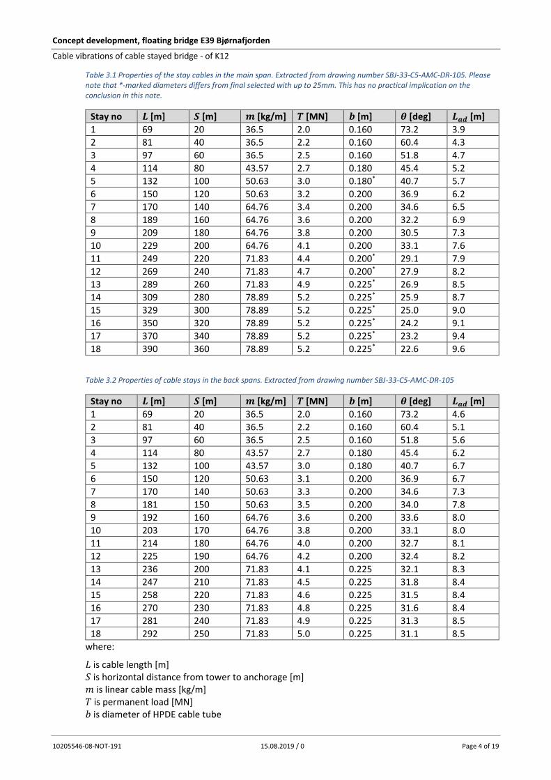
Table 3.1 Properties of the stay cables in the main span. Extracted from drawing number SBJ-33-C5-AMC-DR-105. Please note that *-marked diameters differs from final selected with up to 25mm. This has no practical implication on the conclusion in this note.
Stay no 𝑳 [m] 𝑺 [m] 𝒎 [kg/m] 𝑻 [MN] 𝒃 [m] 𝜽 [deg] 𝑳𝒂𝒅 [m]
1 69 20 36.5 2.0 0.160 73.2 3.9
2 81 40 36.5 2.2 0.160 60.4 4.3
3 97 60 36.5 2.5 0.160 51.8 4.7
4 114 80 43.57 2.7 0.180 45.4 5.2
5 132 100 50.63 3.0 0.180* 40.7 5.7
6 150 120 50.63 3.2 0.200 36.9 6.2
7 170 140 64.76 3.4 0.200 34.6 6.5
8 189 160 64.76 3.6 0.200 32.2 6.9
9 209 180 64.76 3.8 0.200 30.5 7.3
10 229 200 64.76 4.1 0.200 33.1 7.6
11 249 220 71.83 4.4 0.200* 29.1 7.9
12 269 240 71.83 4.7 0.200* 27.9 8.2
13 289 260 71.83 4.9 0.225* 26.9 8.5
14 309 280 78.89 5.2 0.225* 25.9 8.7
15 329 300 78.89 5.2 0.225* 25.0 9.0
16 350 320 78.89 5.2 0.225* 24.2 9.1
17 370 340 78.89 5.2 0.225* 23.2 9.4
18 390 360 78.89 5.2 0.225* 22.6 9.6
Table 3.2 Properties of cable stays in the back spans. Extracted from drawing number SBJ-33-C5-AMC-DR-105
Stay no 𝑳 [m] 𝑺 [m] 𝒎 [kg/m] 𝑻 [MN] 𝒃 [m] 𝜽 [deg] 𝑳𝒂𝒅 [m]
1 69 20 36.5 2.0 0.160 73.2 4.6
2 81 40 36.5 2.2 0.160 60.4 5.1
3 97 60 36.5 2.5 0.160 51.8 5.6
4 114 80 43.57 2.7 0.180 45.4 6.2
5 132 100 43.57 3.0 0.180 40.7 6.7
6 150 120 50.63 3.1 0.200 36.9 6.7
7 170 140 50.63 3.3 0.200 34.6 7.3
8 181 150 50.63 3.5 0.200 34.0 7.8
9 192 160 64.76 3.6 0.200 33.6 8.0
10 203 170 64.76 3.8 0.200 33.1 8.0
11 214 180 64.76 4.0 0.200 32.7 8.1
12 225 190 64.76 4.2 0.200 32.4 8.2
13 236 200 71.83 4.1 0.225 32.1 8.3
14 247 210 71.83 4.5 0.225 31.8 8.4
15 258 220 71.83 4.6 0.225 31.5 8.4
16 270 230 71.83 4.8 0.225 31.6 8.4
17 281 240 71.83 4.9 0.225 31.3 8.5
18 292 250 71.83 5.0 0.225 31.1 8.5
where:
𝐿 is cable length [m] 𝑆 is horizontal distance from tower to anchorage [m] 𝑚 is linear cable mass [kg/m] 𝑇 is permanent load [MN] 𝑏 is diameter of HPDE cable tube

Concept development, floating bridge E39 Bjørnafjorden
Cable vibrations of cable stayed bridge - of K12
10205546-08-NOT-191 15.08.2019 / 0 Page 5 of 19
𝜃 is cable angle with horizontal [deg] 𝐿𝑎𝑑 is distance along cable from anchorage to damper unit [m]
The cable angle 𝜃 with horizontal is obtained as follows:
𝜃 = 𝐴𝑐𝑜𝑠 (𝑆
𝐿) (3.1)
The anchor to damper distance 𝐿𝑎𝑑 is inferred from the vertical anchor to damper distance measured off drawings SBJ-33-C5-AMC-22-DR-103, SBJ-33-C5-AMC-22-DR-104, assuming that all anchor tubes are to terminate at an equal height above the roadway.
Figure 3.2 Say cable tubes for steel main span (left) and concrete back spans (right) indicating assumed vertical distances H between cable anchorage and damper location. Excerpt drawings SBJ-33-C5-AMC-22-DR-103, SBJ-33-C5-AMC-22-DR-104.
𝐿𝑎𝑑 ≈𝑉
𝑠𝑖𝑛 (𝐴𝑐𝑜𝑠 (𝑆𝐿
))
(3.2)
The first eigenfrequency 𝑓1 corresponding to one ½-wave along the cable length is fundamental to stability considerations. 𝑓1 for the main and back span stay cables are calculated following taut string theory (2.3) and displayed in Figure 3.3.
𝑓𝑛 =𝑛
2𝐿√
𝑇
𝑚, 𝑛 = 1 (3.3)
Figure 3.3 First mode eigenfrequencies 𝑓1 (½-wave) of the main and back span stay cables of Bjørnefjorden high bridge.
It is noted that the first mode eigenfrequencies 𝑓1 for the stay cables in the main and back spans falls in the range 1.7 Hz – 0.33 Hz with the longest stay cables having the lowest eigenfrequencies.
1 2 3 4 5 6 7 8 9 10 11 12 13 14 15 16 17 180
0.5
1
1.5
2Main spanBack span
Stay No
Freq
uenc
y [H
z]
V = 3.7 m V = 4.4 m

Concept development, floating bridge E39 Bjørnafjorden
Cable vibrations of cable stayed bridge - of K12
10205546-08-NOT-191 15.08.2019 / 0 Page 6 of 19
4 Stay cable dampers It is common design procedure for cable stayed bridges to be fitted with cable dampers to prevent wind induced cable vibrations. A classical stay cable damper design is to arrange three hydraulic dashpot dampers (pistons) in a 120 degree star configuration as is exemplified by the Freyssinet commercial IRD damper, Figure 4.1.
Figure 4.1 Hydraulic stay cable damper (Freyssinet IRD type). Cross section view (left). External view twin stay cables, Øresundsbron [right).
The compound damping coefficient of the IRD type damper depends on the performance of the individual dashpot units. However, available measurements (Øresundsbron) indicate a damping coefficient in the range 250 kNs/m < 𝐶 < 300 kNs/m for practical installations. The present assessment assumes a damping coefficient 𝐶 = 275 kNs/m.
The effective mechanical damping (rel.-to-crit.) of a stay cable vibrating in the first mode and fitted with a damper close to the anchorage can be estimated from equation (4.1) following /4/.
𝜁𝑚 = 𝜁𝑑 + 𝜁𝑠 =𝐿𝑎𝑑
𝐿
2𝜋𝐿𝑎𝑑𝐶𝑓1𝑇
1 + (2𝜋𝐿𝑎𝑑𝐶𝑓1
𝑇)
2 + 𝜁𝑠 (4.1)
where 𝜁𝑑 represents the effect of the damper and 𝜁𝑠 = 0.001 is the intrinsic structural damping of the stay cable /1/ (rel.-to-crit.). The resulting mechanical damping of the individual stay cable are shown in Figure 4.2, yielding expected damping levels in the range 0.011 – 0.016.
Figure 4.2 Estimated mechanical first mode damping of the main and back span stay cables.
1 2 3 4 5 6 7 8 9 10 11 12 13 14 15 16 17 180
0.01
0.02
0.03
0.04Main spanBack spanIntrinsic damping
Stay No
Dam
ping
[rel
-to-c
rit]

Concept development, floating bridge E39 Bjørnafjorden
Cable vibrations of cable stayed bridge - of K12
10205546-08-NOT-191 15.08.2019 / 0 Page 7 of 19
5 Aerodynamic cable instabilities The aerodynamic cable instabilities mentioned in the introduction (section 1) and their possible effects on the Bjørnafjord high bridge will be discussed and evaluated in the present section.
Known phenomena that may produce stay cable vibrations are as follows:
Dry galloping – an instability associated with assymmetic flow separation on the cable cross sections. The asymetry may be caused either by the cable being in the critical Reynolds number range or by cable surface irregularities.
Ice / sleet galloping – an instability associated with the deposit of ice, snow or sleet along the cabes causing the circular cable cross sections to be assymmetric to the wind.
Rain / wind galloping – an instability associated with rain water draining along the cabes causing the circular cable cross sections to be assymmetric to the wind.
Vortex induced vibrations – an instability associated with the alternating formation and shedding of vortices along the separtion lines at the upper and lower sides of the stay cable.
Common to the above instabilities are that they may be mitigated or delayed to higher wind speeds by introduction of additional mechanical damping to the stay cables.
Before venturing into the assessment a few concepts relating to the wind and stay cable geometry will be defined, Figure 5.1.
Figure 5.1 Definition of relations between the wind and the stay cables.
The angle 𝜙 between the wind direction and the direction of the stay cable known as wind-cable angle 𝜙 is found to be an important parameter for dry galloping. 𝜙 is related to the horizontal wind direction 𝛽 and the cable angle relative to horizontal 𝜃 as follows:
𝑐𝑜𝑠𝜙 = 𝑐𝑜𝑠𝛽𝑐𝑜𝑠𝜃 (5.1)
Thus, for a horizontal cable (𝜃 = 0) 𝜙 = 𝛽. For a vertical cable (𝜃 = 90 deg.) 𝜙 = 90 deg.

Concept development, floating bridge E39 Bjørnafjorden
Cable vibrations of cable stayed bridge - of K12
10205546-08-NOT-191 15.08.2019 / 0 Page 8 of 19
Dry galloping
Dry galloping may occur as the wind flow about an inclined stay cable enters the critical Reynolds´ Number range (2∙105 < 𝑅𝑒 < 3.5∙105). I this range the drag coefficient 𝐶𝐷 drops from a nominal value of 1.2 to approximately 0.4 while a distinctive cross-wind lift coefficient 𝐶𝐿 may develop (𝐶𝐿 ≈∓0.4) due to asymmetric formation and location of the upper and lower separation lines along the cable.
The action of the 𝑅𝑒 dependent lift and drag forces produces a quasi-steady aerodynamic force in the direction of cable movements and thus a resulting negative aerodynamic damping which must be balanced by structural damping if cable movement is to be prevented.
The cable amplitudes due to dry galloping once started cannot be predicted. However, the critical wind speed and the damping necessary for prevention can be estimated from McDonalds aerodynamic damping function 𝑍(𝑅𝑒, 𝜙) which relies on experimental data (wind tunnel tests of inclined circular cylinders), Figure 5.2, /5/. Negative 𝑍(𝑅𝑒, 𝜙) values indicate positive aerodynamic damping adding to the structural damping. Positive 𝑍(𝑅𝑒, 𝜙) values indicate negative aerodynamic damping opposing the structural damping.
The criterion for stability against dry galloping is that the non-dimensional structural damping parameter 𝑍𝑠 is larger than 𝑍(𝑅𝑒, 𝜙):
𝑍𝑠 =𝜁𝑚𝑚𝑓
𝜈𝜌> 𝑍(𝑅𝑒, 𝜙) (5.2)
where 𝜈 = 1.5∙10-5 kgm-1/s is the kinematic viscosity and 𝜌 = 1.25 kg/m-3 is the density of air.
Figure 5.2 McDonalds aerodynamic damping function 𝑍(𝑅𝑒, 𝜙). Smooth flow (left). Corrected for the effects of 6% intensity turbulence (right).
The damping function shown in Figure 5.2, left is valid for smooth flow conditions for which the underling wind tunnel tests were carried out. Introducing turbulence has the effect of decreasing the Reynolds' Numbers for the critical range as well as making the transition in 𝐶𝐷 from sub-critical to critical Reynolds' numbers more gradual. Correction of the smooth flow data according to ESDU /6/ to turbulent flow having 6% turbulence intensity typical of costal conditions yields reductions in the maximum damping and the corresponding Reynolds' Number, Figure 5.2, right.
From the left-hand graph (smooth flow) it is noted that maximum value of 𝑍𝑚𝑎𝑥 = 40∙103 for 𝑅𝑒𝑚𝑎𝑥 = 3.3∙105, where as the right-hand graph (turbulent flow) indicates a maximum value of 𝑍𝑚𝑎𝑥 = 16∙103 for 𝑅𝑒𝑚𝑎𝑥 = 1.6∙105. The corresponding wind-cable angle is 𝜙𝑚𝑎𝑥 = 83 deg.
With the aid of (5.1) the wind direction 𝛽 relative to the cable planes for critical dry galloping conditions can be estimated for all cable stays Figure 5.3.

Concept development, floating bridge E39 Bjørnafjorden
Cable vibrations of cable stayed bridge - of K12
10205546-08-NOT-191 15.08.2019 / 0 Page 9 of 19
It is noted that critical conditions are expected for all cables in the interval 65 deg. < 𝛽 < 82 deg. With the NE alignment of the bridge axis this coincides with the prevailing westerly winds at the bridge site.
Figure 5.3 Wind direction 𝛽 for maximum dry galloping excitation relative to the cable planes for the main and back span cable stays.
The critical wind speeds 𝑉𝐶𝐺 for dry galloping of the main and back span cables are calculated from the critical Reynolds' Numbers 𝑅𝑒𝑚𝑎𝑥 = 3.3∙105, 𝑅𝑒𝑚𝑎𝑥 = 1.6∙105 yielding maximum galloping excitation in smooth and turbulent flow:
𝑉𝐶𝐺 =𝑅𝑒𝑚𝑎𝑥𝜈
𝑏 (5.3)
The estimated dry galloping wind speeds for the main and back span stay cables are shown in Figure 5.4 along with the EN1991-1-4 galloping criterion (1.1).
Figure 5.4 Calculated critical wind speeds for maximum dry galloping excitation of all cables in smooth flow.
From Figure 5.4 it is noted that the estimated dry galloping wind speeds for all stay cables falls below the EN1991-1-4 criterion demonstrating that cable dampers are necessary to prevent or delay the onset of dry galloping.
1 2 3 4 5 6 7 8 9 10 11 12 13 14 15 16 17 180
15
30
45
60
75
90
Main spanBack span
Stay No
Win
d di
rect
ion
[deg
] rel
ativ
e to
cab
le p
lane
s
1 2 3 4 5 6 7 8 9 10 11 12 13 14 15 16 17 180
10
20
30
40
50
60Main span, smoothBack span, smoothMain span, turbulentBack span, turbulentEN1991-1-4 criterion
Stay No
Gal
lopi
ng w
ind
spee
ds V
cg [m
/s]

Concept development, floating bridge E39 Bjørnafjorden
Cable vibrations of cable stayed bridge - of K12
10205546-08-NOT-191 15.08.2019 / 0 Page 10 of 19
Calculated non-dimensional structural cable damping parameters 𝑍𝑠 according to eqn. (4.2) assuming intrinsic cable damping only (𝜁𝑠 = 0.001) and comparison to 𝑍𝑚𝑎𝑥 for smooth and turbulent flow are shown in Figure 5.6.
Figure 5.5 Calculated non-dimensional cable damping parameters and comparison to maximum smooth and turbulent
flow values for the main and back span cable stays for intrinsic cable damping 𝜁𝑠 = 0.001.
From Figure 5.5 it is noted that 𝑍𝑠 falls below 𝑍𝑚𝑎𝑥 for smooth flow as well as for turbulent flow conditions thus dry galloping is expected in case the stay cables are not equipped with cable dampers.
Inclusion of cable dampers will increase the mechanical damping substantially as shown in Figure 4.2, and will improve the dry galloping performance considerably as shown in Figure 5.6.
Figure 5.6 Calculated non-dimensional cable damping parameters and comparison to maximum smooth and turbulent flow values for the main and back span cable stays including damper units.
From Figure 5.6 it is noted that all stay cables are prone to dry galloping I smooth flow conditions with the structural damping parameter 𝑍𝑠 of the longest cables falling the most below the critical 𝑍𝑚𝑎𝑥 = 40∙103 (green horizontal line). For turbulent flow conditions 𝑍𝑠 > 𝑍𝑚𝑎𝑥 = 16∙103 for all stay cables. Hence dry galloping should not pose a problem if all stay cables are equipped with dampers having sufficient capacity.
1 2 3 4 5 6 7 8 9 10 11 12 13 14 15 16 17 180
1
2
3
4
5Zs, Main spanZs, Back spanZmax, smoothZmax, turbulent
Stay No
Non
-dim
dam
ping
Zm
ax, Z
s x 1
0-̂4
1 2 3 4 5 6 7 8 9 10 11 12 13 14 15 16 17 180
1
2
3
4
5Zs, Main spanZs, Back spanZmax, smoothZmax, turbulent
Stay No
Non
-dim
dam
ping
Zm
ax, Z
s x 1
0-̂4

Concept development, floating bridge E39 Bjørnafjorden
Cable vibrations of cable stayed bridge - of K12
10205546-08-NOT-191 15.08.2019 / 0 Page 11 of 19
Galloping due to cable surface irregularities
New research into the galloping of cylindrical cable surface elements has revealed that small deviations from the perfect circular cross section shape may cause substantial cross wind lift forces in the critical Reynolds number range 2∙105 < 𝑅𝑒 < 3.5∙105. Wind tunnel measurements of the lift and drag coefficients as function of 𝑅𝑒 with the inflow angle 𝛼 as parameter for a commercial HDPE tube having a diameter of 160 mm with ± 1 mm deviations, /7/, is reproduced in Figure 5.7.
Figure 5.7 Variations of lift (upper) and drag (lower) coefficients as function of 𝑅𝑒 and inflow angle 𝛼 for a commercial stay cable HPDE tube. Reproduced from /8/.
The data in Figure 5.7 may be interpreted to result in galloping by two different mechanisms:
1. Classical den Hartog galloping due to a negative gradient of the lift coefficient as function of inflow angle.
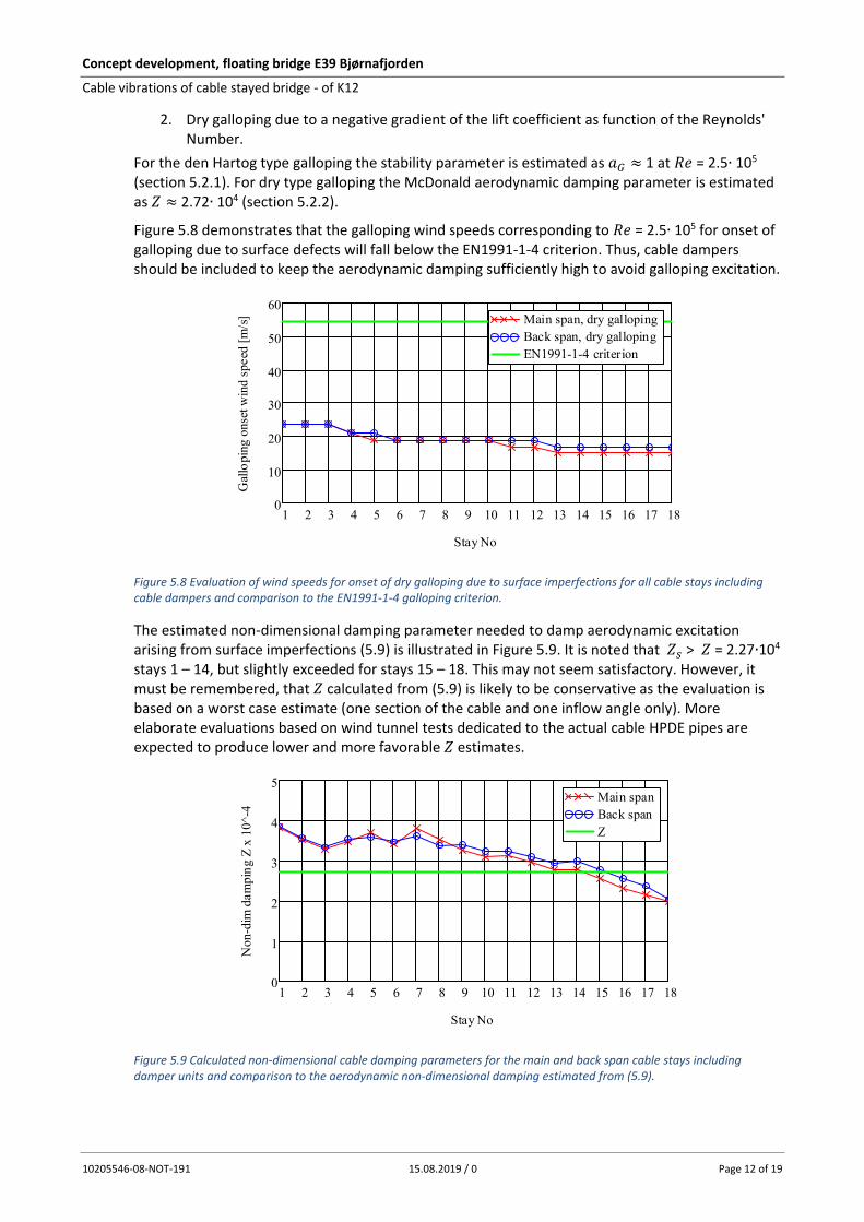
Concept development, floating bridge E39 Bjørnafjorden
Cable vibrations of cable stayed bridge - of K12
10205546-08-NOT-191 15.08.2019 / 0 Page 12 of 19
2. Dry galloping due to a negative gradient of the lift coefficient as function of the Reynolds' Number.
For the den Hartog type galloping the stability parameter is estimated as 𝑎𝐺 ≈ 1 at 𝑅𝑒 = 2.5∙ 105 (section 5.2.1). For dry type galloping the McDonald aerodynamic damping parameter is estimated as 𝑍 ≈ 2.72∙ 104 (section 5.2.2).
Figure 5.8 demonstrates that the galloping wind speeds corresponding to 𝑅𝑒 = 2.5∙ 105 for onset of galloping due to surface defects will fall below the EN1991-1-4 criterion. Thus, cable dampers should be included to keep the aerodynamic damping sufficiently high to avoid galloping excitation.
Figure 5.8 Evaluation of wind speeds for onset of dry galloping due to surface imperfections for all cable stays including cable dampers and comparison to the EN1991-1-4 galloping criterion.
The estimated non-dimensional damping parameter needed to damp aerodynamic excitation arising from surface imperfections (5.9) is illustrated in Figure 5.9. It is noted that 𝑍𝑠 > 𝑍 = 2.27∙104 stays 1 – 14, but slightly exceeded for stays 15 – 18. This may not seem satisfactory. However, it must be remembered, that 𝑍 calculated from (5.9) is likely to be conservative as the evaluation is based on a worst case estimate (one section of the cable and one inflow angle only). More elaborate evaluations based on wind tunnel tests dedicated to the actual cable HPDE pipes are expected to produce lower and more favorable 𝑍 estimates.
Figure 5.9 Calculated non-dimensional cable damping parameters for the main and back span cable stays including damper units and comparison to the aerodynamic non-dimensional damping estimated from (5.9).
1 2 3 4 5 6 7 8 9 10 11 12 13 14 15 16 17 180
10
20
30
40
50
60Main span, dry gallopingBack span, dry gallopingEN1991-1-4 criterion
Stay No
Gal
lopi
ng o
nset
win
d sp
eed
[m/s
]
1 2 3 4 5 6 7 8 9 10 11 12 13 14 15 16 17 180
1
2
3
4
5Main spanBack spanZ
Stay No
Non
-dim
dam
ping
Z x
10^
-4

Concept development, floating bridge E39 Bjørnafjorden
Cable vibrations of cable stayed bridge - of K12
10205546-08-NOT-191 15.08.2019 / 0 Page 13 of 19
5.2.1 den Hartog type galloping
From Figure 5.7 upper graph it is noted that the lift coefficient 𝐶𝐿 at 𝑅𝑒 = 2.5∙ 105 varies substantially as function of the inflow angle 𝛼 whereas the drag coefficient 𝐶𝐷 displays relatively little variation. Estimation of the galloping stability parameter 𝑎𝐺 at an inflow angle 𝛼 ≈ 750 based on 𝐶𝐿, 𝐶𝐷 data for 𝛼 = 600 ( ), 𝛼 = 900 ( ):
𝑎𝐺 ≈ − [𝑑𝐶𝐿
𝑑𝛼+ 𝐶𝐷] = − [
𝐶𝐿,90 𝑑𝑒𝑔 − 𝐶𝐿,60 𝑑𝑒𝑔
90 − 60 ∙ 57.3 + 𝐶𝐷]
= − [−0.5 − 0.3
30∙ 57.3 + 0.55] ≅ 1.0
(5.4)
Following (5.4) galloping excitation due to cable surface irregularities may result in similar galloping excitation as ice accretion at critical 𝑅𝑒 (section 5.4).
Following EN1991-1-4 the wind speed for onset of den Hartog galloping can be estimated as:
𝑉𝐶𝐺 =2𝑆𝑐
𝑎𝐺𝑓1𝑏 =
8𝜋𝑚𝑒𝑓1
𝑎𝐺𝜌𝑏 (5.5)
where the effective mass 𝑚𝑒= 𝑚 for sinusoidal cable mode shapes.
5.2.2 dry type galloping
Dry type (or Reynolds' Number dependent) galloping is governed by McDonalds damping function 𝑍(𝑅𝑒, 𝜙) which, for a circular cylindrical cable, may be expressed as /6/:
𝑍(𝑅𝑒, 𝜙) =𝑅𝑒
16𝜋[−ℎ(𝐶𝐷) + √𝑔(𝐶𝐷)2 + 𝑔(𝐶𝐿)2 − ℎ(𝐶𝐿)2] (5.6)
with auxiliary functions:
ℎ(𝐶𝐹) = 𝑔(𝐶𝐹) +2𝐶𝐹
𝑠𝑖𝑛𝜙
𝑔(𝐶𝐹) = 𝐶𝐹 (2𝑠𝑖𝑛𝜙 −1
𝑠𝑖𝑛𝜙) +
𝜕𝐶𝐹
𝜕𝜙𝑐𝑜𝑠𝜙 +
𝜕𝐶𝐹
𝜕𝑅𝑒𝑅𝑒 ∙ 𝑠𝑖𝑛𝜙
(5.7)
with 𝐶𝐹 = 𝐶𝐷 or 𝐶𝐿.
Assuming 𝜙 ≈ 𝜙𝑚𝑎𝑥 ≈ 𝜋 2⁄ and that the force coefficients 𝐶𝐷, 𝐶𝐿 vary slowly as function of 𝜙 (𝜕𝐶𝐹 𝜕𝜙⁄ ≈ 0) the auxiliary functions (5.7) can be simplified to read:
ℎ(𝐶𝐹) = 3𝐶𝐹 +𝜕𝐶𝐹
𝜕𝑅𝑒𝑅𝑒 𝑔(𝐶𝐹) = 𝐶𝐹 +
𝜕𝐶𝐹
𝜕𝑅𝑒𝑅𝑒 (5.8)
which In turn yields the following approximate form of 𝑍(𝑅𝑒):
𝑍(𝑅𝑒) ≈𝑅𝑒
16𝜋[− (3𝐶𝐷 +
𝜕𝐶𝐷
𝜕𝑅𝑒𝑅𝑒) + √(𝐶𝐷 +
𝜕𝐶𝐷
𝜕𝑅𝑒𝑅𝑒)
2
− 4𝐶𝐿 (2𝐶𝐿 +𝜕𝐶𝐿
𝜕𝑅𝑒𝑅𝑒)] (5.9)
With reference to Figure 5.7 it is noted that 𝐶𝐿 exhibit strong negative gradients as function of 𝑅𝑒 for inflow angles 𝛼 = 00 or 𝛼 = 1200.
Evaluation of the 𝐶𝐷, 𝐶𝐿 gradients and 𝑍 for the Reynolds' Number range 2.4∙ 105 < 𝑅𝑒 < 2.6∙ 105 for 𝛼 = 1200 (following the red dashed tangent line in Figure 5.7) is outlined in Table 5.1.
In closing it should be noted that the evaluations in section 5.2.1 and 5.2.2 are based on pressure measurements made at one section along a commercial HPDE cable duct. Surface imperfections may vary along the span of the duct and lead to a pronounced span wise variation of 𝐶𝐷 and 𝐶𝐿 similar to the variation with inflow angle demonstrated in Figure 5.7. Such variations will decrease the tendencey for galloping or increase the onset wind speed.
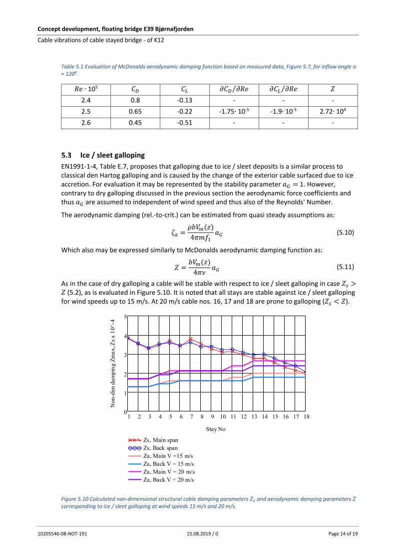
Concept development, floating bridge E39 Bjørnafjorden
Cable vibrations of cable stayed bridge - of K12
10205546-08-NOT-191 15.08.2019 / 0 Page 14 of 19
Table 5.1 Evaluation of McDonalds aerodynamic damping function based on measured data, Figure 5.7, for inflow angle 𝛼 = 1200.
𝑅𝑒 ∙ 105 𝐶𝐷 𝐶𝐿 𝜕𝐶𝐷 𝜕𝑅𝑒⁄ 𝜕𝐶𝐿 𝜕𝑅𝑒⁄ 𝑍
2.4 0.8 -0.13 - - -
2.5 0.65 -0.22 -1.75∙ 10-5 -1.9∙ 10-5 2.72∙ 104
2.6 0.45 -0.51 - - -
Ice / sleet galloping
EN1991-1-4, Table E.7, proposes that galloping due to ice / sleet deposits is a similar process to classical den Hartog galloping and is caused by the change of the exterior cable surfaced due to ice accretion. For evaluation it may be represented by the stability parameter 𝑎𝐺 = 1. However, contrary to dry galloping discussed in the previous section the aerodynamic force coefficients and thus 𝑎𝐺 are assumed to independent of wind speed and thus also of the Reynolds' Number.
The aerodynamic damping (rel.-to-crit.) can be estimated from quasi steady assumptions as:
𝜁𝑎 =𝜌𝑏𝑉𝑚(𝑧)
4𝜋𝑚𝑓1𝑎𝐺 (5.10)
Which also may be expressed similarly to McDonalds aerodynamic damping function as:
𝑍 =𝑏𝑉𝑚(𝑧)
4𝜋𝜈𝑎𝐺 (5.11)
As in the case of dry galloping a cable will be stable with respect to ice / sleet galloping in case 𝑍𝑠 >𝑍 (5.2), as is evaluated in Figure 5.10. It is noted that all stays are stable against ice / sleet galloping for wind speeds up to 15 m/s. At 20 m/s cable nos. 16, 17 and 18 are prone to galloping (𝑍𝑠 < 𝑍).
Figure 5.10 Calculated non-dimensional structural cable damping parameters 𝑍𝑠 and aerodynamic damping parameters 𝑍 corresponding to ice / sleet galloping at wind speeds 15 m/s and 20 m/s.
1 2 3 4 5 6 7 8 9 10 11 12 13 14 15 16 17 180
1
2
3
4
5
Zs, Main spanZs, Back spanZa, Main V =15 m/sZa, Back V = 15 m/sZa, Main V = 20 m/sZa, Back V = 20 m/s
Stay No
Non
-dim
dam
ping
Zm
ax, Z
s x 1
0-̂4

Concept development, floating bridge E39 Bjørnafjorden
Cable vibrations of cable stayed bridge - of K12
10205546-08-NOT-191 15.08.2019 / 0 Page 15 of 19
The evaluation presented in Figure 5.10 is only strictly valid for stay cables with ice accretions along the entre cable length. If ice accretion is restricted to a limited part of the cable the galloping excitation will be less and in part counterbalanced by positive aerodynamic damping along the parts of the cables free of ice / sleet.
It is possible to make allowance for the partial ice / sleet coverage assuming a limited extent of cable for which (5.10) applies, whereas the ice / sleet free parts receives aerodynamic damping associated with a circular cylinder in forced cross-wind oscillations. In this case (5.11) is modified to read:
𝑍 =𝑏𝑉𝑚(𝑧)
4𝜋𝜈𝐿[𝑎𝐺 ∫ 𝜑2(𝑥)𝑑𝑥 − 𝐶𝐷 ∫ 𝜑2(𝑥)𝑑𝑥
𝐿2
−∆
0
𝐿2
+∆
𝐿2
−∆
] (5.12)
where 𝐿 is cable length, 2∆ is ice / sleet covered length about the cable midpoint and 𝜑(𝑥) is the cable mode shape taken to be equal to ½ sine wave.
Figure 5.11 shows the development of 𝑍 as function of wind speed and the percentage of ice / sleet covered length compared to 𝑍𝑠 for stay cable no. 18 in the main span. It is noted that cable no. 18 is expected to stable up to wind speeds of about 15 m/s if completely covered by ice / sleet (𝑍𝑠 ≥ 𝑍). If the ice coverage is reduced to about 50% the galloping wind speed is increased to 20 m/s. For ice / sleet covered lengths up to 22%, cable 18 is expected to be stable up to the EN1991-1-4 requirement of 54.3 m/s.
Figure 5.11 Non-dimensional damping parameters as function of wind speed and ice / sleet cover deposited symmetrically about the cable midpoint. Stay cable equipped with mechanical damper unit (section 4).
Rain / wind galloping
Based on observations made during the Erasmus Bridge cable vibration incident, Rotterdam, November 1994, /9/, the following model has been proposed for the maximum amplitude 𝑎 of stay-cables (midpoint for 1 mode) excited by rain / wind:
𝑎 = (𝑉𝑚(𝑧)
2𝜋𝑓1) √
8
6𝜖√𝑌 −
8𝜋𝑓1(𝜁𝑠 + 𝜁𝑑)
𝜌𝑉𝑚(𝑧)𝑏 (5.13)
where:
𝜖 = 8.0 is a non-linearity parameter
𝑌 = 1.2 aerodynamic excitation [m]
𝜌 = 1.25 kgm-3 is air density
0 0.1 0.2 0.3 0.4 0.5 0.6 0.7 0.8 0.9 10
1
2
3
4
5Zs, Main span cable 18Z, V = 15 m/sZ, V = 20 m/sZ, V = 54.3 m/s
Iced up / total cable length
Non
-dim
dam
ping
Zs,
Z x
10^
-4

Concept development, floating bridge E39 Bjørnafjorden
Cable vibrations of cable stayed bridge - of K12
10205546-08-NOT-191 15.08.2019 / 0 Page 16 of 19
The parameters 𝜖 = 8.0, 𝑌 = 1.2 m assumed above are slightly conservative as compared to 𝜖 = 9.4, 𝑌 = 0.86 m originally derived for the Erasmus Bridge.
Evidence from incidents of rain / wind oscillations of stay-cables suggests that the oscillations tends to be strongest for wind speeds of about 15 m/s. Above this wind speed the water rivulet responsible for the cable oscillations tends to be blown off the cable surface thus stopping the excitation.
Plots showing the calculated maximum amplitudes for the main and back span cables with and
without the proposed cable dampers are shown in graphical form in Figure 5.12, Figure 5.13
assuming a maximum wind speed of 15 m/s. The estimated amplitudes are compared to
acceptance criterion 𝐴𝑚𝑎𝑥 < 𝐿 1700⁄ (1.3).
Figure 5.12 Predicted maximum (mid span) cable amplitudes due to rain / wind galloping at V = 15 m/s and comparison to criterion. Cables without dampers.
Figure 5.13 Predicted maximum (mid span) cable amplitudes due to rain / wind galloping at V = 15 m/s and comparison to criterion. Cables including dampers.
From Figure 5.12 it is noted that predicted maximum cable vibrations due to rain / wind galloping of the cables without dampers are expected to reach amplitudes in the range 0.5 m – 3.0 m thus exceeding the acceptance criterion. When including the mechanical dampers all cables are predicted to be stable against rain / wind galloping, 𝑎 ≈ 0.
1 2 3 4 5 6 7 8 9 10 11 12 13 14 15 16 17 180
1
2
3
4
5Main spanBack spanL/1700 Main spanL/1700 BAck span
Stay No
Max
imum
am
plitu
de a
[m]
1 2 3 4 5 6 7 8 9 10 11 12 13 14 15 16 17 180
0.1
0.2
0.3
0.4
0.5Main spanBack spanL/1700 Main spanL/1700 BAck span
Stay No
Max
imum
am
plitu
de a
[m]

Concept development, floating bridge E39 Bjørnafjorden
Cable vibrations of cable stayed bridge - of K12
10205546-08-NOT-191 15.08.2019 / 0 Page 17 of 19
6 Vortex shedding excitation Vortex shedding excitation of a stay cable may occur when the frequency 𝑓𝑣𝑡𝑥 of vortices shed in the wake of the cable coincides with one of the eigenfrequencies 𝑓𝑛 (3.3) of the cable, 𝑓𝑣 = 𝑓𝑛.
Following EN1991-1-4 the vortex shedding frequency is related to the wind speed and cable cross section diameter 𝑏 through the Strouhal Number:
𝑆𝑡 =𝑏𝑓𝑣
𝑉= 0.18 (5.14)
Thus, the wind speeds for vortex induced vibrations of the stay cables is obtained as:
𝑉𝑐𝑟𝑖𝑡,𝑛 =𝑏𝑓𝑛
𝑆𝑡=
𝑏𝑓𝑛
0.18 (5.15)
Yielding the lowest critical wind speeds for the first modes of the stay cables ( 𝑓1 ), Figure 6.1.
Figure 6.1 First mode critical wind speeds for vortex shedding excitation for all stay cables in main and back spans.
Figure 6.1 demonstrates that the first mode critical wind speeds fall in the range 0.5 m/s - 1.5 m/s thus 𝑉𝑐𝑟𝑖𝑡,1 < 54.3 m/s following (1.2). The analysis then proceeds to evaluate expected amplitudes
to be compare to (1.3).
For structures capable of responding in multiple modes (such as taut cables) EN1991-1-4 proposes the following expression (Method 1) for calculation of maximum amplitudes 𝑎 due to vortex shedding excitation:
𝑎
𝑏=
1
𝑆𝑡2
1
𝑆𝑐𝐾 ∙ 𝐾𝑤 ∙ 𝐶𝑙𝑎𝑡 =
1
0.182
𝜌𝑏2
4𝜋(𝜁𝑠 + 𝜁𝑑)𝐾 ∙ 𝐾𝑤 ∙ 𝐶𝑙𝑎𝑡 (5.16)
with a recommended 𝐶𝑙𝑎𝑡 = 0.7 for 𝑅𝑒 < 2.5∙ 105 (sub-critical).
For sinusoidal mode shapes 𝐾= 0.101 and:
𝐾𝑤 = 𝑐𝑜𝑠 [𝜋
2(1 −
𝑐𝑛𝑏𝑛
𝐿)] (5.17)
With the correlation length factor in the range 6 < 𝑐𝑛 < 12 depending on the resulting amplitudes. For the present evaluation the more conservative value 𝑐𝑛= 12 is adopted. The resulting maximum amplitudes are shown in Figure 6.2, Figure 6.3 and compared to the acceptance criterion (1.3).
1 2 3 4 5 6 7 8 9 10 11 12 13 14 15 16 17 180
0.5
1
1.5
2Main span, dry gallopingBack span, dry galloping
Stay No
Firs
t mod
e cr
itica
l win
d sp
eeds
[m/s]

Concept development, floating bridge E39 Bjørnafjorden
Cable vibrations of cable stayed bridge - of K12
10205546-08-NOT-191 15.08.2019 / 0 Page 18 of 19
Figure 6.2 Maximum vortex induced amplitudes for 1`th and 10´th mode of the main and back span stay cables without dampers.
Figure 6.3 Maximum vortex induced amplitudes for 1`th and 10´th mode of the main and back span stay cables including dampers.
From Figure 6.2 it is noted that predicted 10'th mode amplitudes for the longer cable stay are exceeding the criterion in case the cables are not equipped with dampers. If the stay cables are equipped with dampers, Figure 6.3, all maximum amplitudes fall below the acceptance criterion.
1 2 3 4 5 6 7 8 9 10 11 12 13 14 15 16 17 180
0.2
0.4
0.6
0.8
1
Main span, mode 1Back span, mode 1Main span, mode 10Back span, mode 10L/1700 Main spanL/1700 Back span
Stay No
Max
imum
am
plitu
de a
[m]
1 2 3 4 5 6 7 8 9 10 11 12 13 14 15 16 17 180
0.1
0.2
0.3
0.4
0.5
Main span, mode 1Back span, mode 1Main span, mode 10Back span, mode 10L/1700 Main spanL/1700 Back span
Stay No
Max
imum
am
plitu
de a
[m]

Concept development, floating bridge E39 Bjørnafjorden
Cable vibrations of cable stayed bridge - of K12
10205546-08-NOT-191 15.08.2019 / 0 Page 19 of 19
7 Conclusion and recommendation The present technical note has evaluated the risk of wind induced stay cable vibrations of the Bjørnafjorden high bridge.
It is found that the stay cables are likely to be free of unacceptable wind related vibrations in case they are equipped damper units having a damper capacity similar to currently available commercial designs. In case dampers are omitted, the stay cables are likely to receive unacceptable vibrations when exposed to winds above, say, 10 m/s at deck level.
The prediction models applied for the present assessment are based on data obtained for smooth surface stay cables and smooth cylinders. Contemporary HPDE pipe surface modifications such as helical fillets or dimples are not covered by the present analysis and may bias the outcome of the assessment. In view of this uncertainty it is recommended to verify the aerodynamic properties of the stay cable pipes by means of wind tunnel tests as part of the detailed design of the bridge.
8 References
/1/ Eurocode EN1991-1-4: Action on structures – Part 1-4: General actions – Wind actions. 2ed, 2007.
/2/ 10205546-08-NOT-184_0: Aerodynamic stability of K12, 15-08-2019.
/3/ Acceptance of stay cable systems using pre-stressing steels. fib Recommendation Bulletin 30:2005.
/4/ Krenk. S, Høgsberg, J. R.: Damping of cables by a transverse force. Journal of Engineering Mechanics, ASCE, April 2005.
/5/ McDonald, J. H. G.: Quasi-steady analysis of 2dof inclined cable galloping in the critical Reynolds´ Number range. Sixth International Symposium on Cable Dynamics, Charleston, SC, USA. 19-22 Sept. 2005.
/6/ ESDU, Item 80025C, 1986: Mean forces, pressures and flow field velocities for circular cylindrical structures: Single cylinder with two-dimensional flow.
/7/ Matteoni, G., Georgakis, C.T.: Effects of bridge cable surface roughness and cross-sectional distorsion on aerodynamic force coefficients. Proceedings, International Conference on Wind Engineering, ICWE13, 10-15 June 2011, Amsterdam, The Netherlands.
/8/ Guerts, C., Vrouwenvelder, T., Staalduinen, P. v.: Numerical modelling of rain-wind induced vibration. Erasmus Bridge, Rotterdam. SEI, Vol 8, Nr. 2, May 1998.

Concept development, floating bridge
E39 Bjørnafjorden
Appendix E – Enclosure 12
10205546-08-NOT-192
CFD analysis of K12
0 15.08.2019 Final issue M. Papinutti R. M. Larssen S. E. Jakobsen
REV. DATE DESCRIPTION PREPARED BY CHECKED BY APPROVED BY
MEMO
PROJECT Concept development, floating bridge E39 Bjørnafjorden
DOCUMENT CODE 10205546-08-NOT-192
CLIENT Statens vegvesen ACCESSIBILITY Restricted
SUBJECT CFD analysis of K12 PROJECT MANAGER Svein Erik Jakobsen
TO Statens vegvesen PREPARED BY Mitja Papinutti
COPY TO RESPONSIBLE UNIT AMC
SUMMARY
This document presents a summary of aerodynamic values for the final design cross section K12. The numerical analysis was performed with the Computational Fluid Dynamics (CFD) tool to calculate the bridge deck aerodynamics. The Discrete Vortex Method (DVM) method inside commercial software package RM Bridge was used in these investigations. The CFD model is calibrated and compared to the wind tunnel tests from 3rd phase of BJF project. Details are available in the report 10205546-08-NOT-062 CFD Analysis of cross-sections.
This memo presents results on K12 cross-section for both Quays-Steady State (QSS) and the unsteady flutter derivatives. A good match between the wind tunnel and numerically extracted results is observed, thus offers the required confidence level of the results. Provided validation also confirms the CFD extraction techniques. The aerodynamic performance of the selected cross section for the final design K12, and are compared to reference previous initial design cross section SS1.

Concept development, floating bridge E39 Bjørnafjorden
CFD analysis of K12
10205546-08-NOT-192 15.08.2019 / 0 Page 2 of 10
Table of Contents 1 About CFD .................................................................................................................................. 3
2 Cross section geometry .............................................................................................................. 4
3 Quasi-steady state coefficients extraction ................................................................................. 5
4 Flutter derivatives ...................................................................................................................... 7
5 Conclusion ................................................................................................................................ 10

Concept development, floating bridge E39 Bjørnafjorden
CFD analysis of K12
10205546-08-NOT-192 15.08.2019 / 0 Page 3 of 10
1 About CFD In RM Bridge, a CFD module is available for computing the aerodynamic coefficients CD, CL, CM of different cross-sections. The plane airflow around the obstacle can be described by the two-dimensional Navier-Stokes equation. The assumption of incompressible fluids with constant viscosity is applied, resulting in the vorticity transport equations defined by:
𝜕𝜔
𝜕+ (𝒖 ⋅ 𝛻)𝜔 = 𝑣𝛥𝜔
Where
𝒖 = is the velocity of the fluid 𝜔 = is the curl of this velocity (vorticity) 𝑣 = is the kinematical viscosity of air (0.000015 m2/s at 20°C)
This equation is numerically solved for the open flow boundary conditions and deck wall assumption. The method used is the Discrete Vortex Method (DVM). The forces are calculated by the pressure integration of the two-dimensional cross-section, as a result of velocity filed around the deck depicted in Figure 1.
Figure 1: Velocity wind field around the deck and particle flow tracking, RM Bridge CFD tool.

Concept development, floating bridge E39 Bjørnafjorden
CFD analysis of K12
10205546-08-NOT-192 15.08.2019 / 0 Page 4 of 10
2 Cross section geometry The K12 cross section was modeled together with the 1.6m wide wind nose. The nose improves the aerodynamic performance introduction more controlled flow separation. The details of simplified fences and railings have were included in this investigation. The asphalt layer has been added to better simulated the top deck pressure redistribution. The cross-section dimension of K12 are depicted in Figure 2. The results are compared to the previous design cross-section SS1, depicted in Figure 3.
Figure 2: Finite element model of K12 cross section, used as final design cross section.
Figure 3: Finite element model of SS1 cross section, used for previous design cross section.
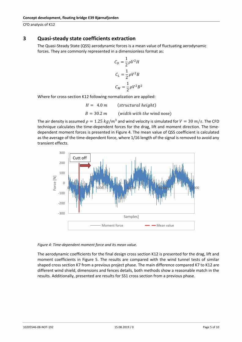
Concept development, floating bridge E39 Bjørnafjorden
CFD analysis of K12
10205546-08-NOT-192 15.08.2019 / 0 Page 5 of 10
3 Quasi-steady state coefficients extraction The Quasi-Steady State (QSS) aerodynamic forces is a mean value of fluctuating aerodynamic forces. They are commonly represented in a dimensionless format as:
𝐶𝐷 =1
2𝜌𝑉2𝐻
𝐶𝐿 =1
2𝜌𝑉2𝐵
𝐶𝑀 =1
2𝜌𝑉2𝐵2
Where for cross-section K12 following normalization are applied:
𝐻 = 4.0 𝑚 (𝑠𝑡𝑟𝑢𝑐𝑡𝑢𝑟𝑎𝑙 ℎ𝑒𝑖𝑔ℎ𝑡)
𝐵 = 30.2 𝑚 (𝑤𝑖𝑑𝑡ℎ 𝑤𝑖𝑡ℎ 𝑡ℎ𝑒 wind nose)
The air density is assumed 𝜌 = 1.25 𝑘𝑔/𝑚3 and wind velocity is simulated for 𝑉 = 30 𝑚/𝑠. The CFD technique calculates the time-dependent forces for the drag, lift and moment direction. The time-dependent moment forces is presented in Figure 4. The mean value of QSS coefficient is calculated as the average of the time-dependent force, where 1/16 length of the signal is removed to avoid any transient effects.
Figure 4: Time-dependent moment force and its mean value.
The aerodynamic coefficients for the final design cross section K12 is presented for the drag, lift and moment coefficients in Figure 5. The results are compared with the wind tunnel tests of similar shaped cross section K7 from a previous project phase. The main difference compared K7 to K12 are different wind shield, dimensions and fences details, both methods show a reasonable match in the results. Additionally, presented are results for SS1 cross section from a previous phase.
-300
-200
-100
0
100
200
300
0 5000 10000 15000 20000Forc
e [N
]
Samples]
Moment force Mean value
Cutt off
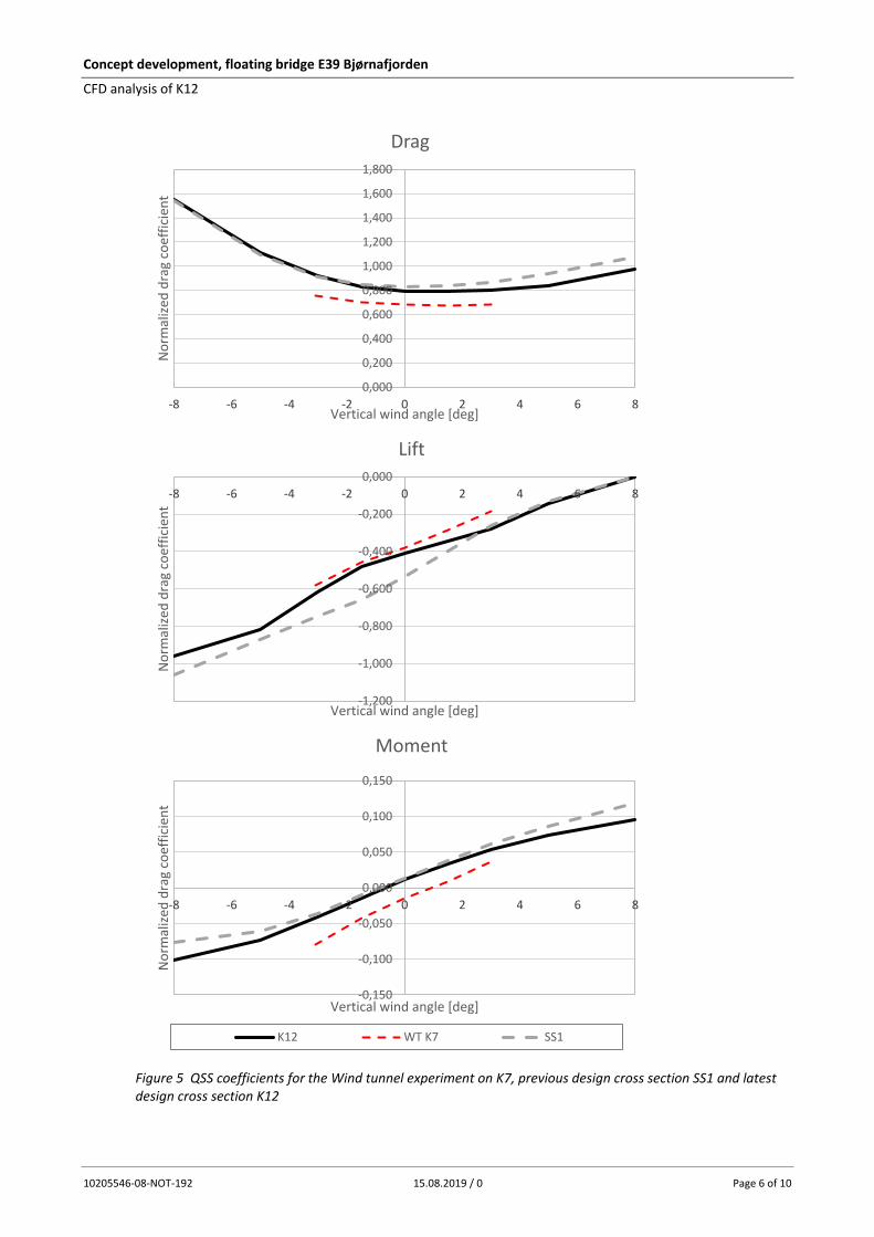
Concept development, floating bridge E39 Bjørnafjorden
CFD analysis of K12
10205546-08-NOT-192 15.08.2019 / 0 Page 6 of 10
Figure 5 QSS coefficients for the Wind tunnel experiment on K7, previous design cross section SS1 and latest design cross section K12
0,000
0,200
0,400
0,600
0,800
1,000
1,200
1,400
1,600
1,800
-8 -6 -4 -2 0 2 4 6 8
No
rmal
ized
dra
g co
effi
cien
t
Vertical wind angle [deg]
Drag
-1,200
-1,000
-0,800
-0,600
-0,400
-0,200
0,000
-8 -6 -4 -2 0 2 4 6 8
No
rmal
ized
dra
g co
effi
cien
t
Vertical wind angle [deg]
Lift
-0,150
-0,100
-0,050
0,000
0,050
0,100
0,150
-8 -6 -4 -2 0 2 4 6 8
No
rmal
ized
dra
g co
effi
cien
t
Vertical wind angle [deg]
Moment
K12 WT K7 SS1

Concept development, floating bridge E39 Bjørnafjorden
CFD analysis of K12
10205546-08-NOT-192 15.08.2019 / 0 Page 7 of 10
4 Flutter derivatives The Scanlan flutter derivatives are defined as motion dependent values. They are normalized values and are frequency dependent. For the two-dimensional aeroelastic cross-section following notation is commonly used for aeroelastic damping:
𝐶𝑠𝑒 =𝜌𝐵2
2ω [
𝐻1∗ 𝐵𝐻2
∗
𝐵𝐴1∗ 𝐵2𝐴2
∗ ]
and aeroelastic stiffness:
𝐾𝑠𝑒 =𝜌𝐵2
2ω2 [
𝐻4∗ 𝐵𝐻3
∗
𝐵𝐴4∗ 𝐵2𝐴3
∗ ]
The flutter derivatives for vertical motion 𝐻1−4
∗ and for pinch rotations 𝐴1−4∗ are expressed with
dimensionless reduced velocity �̅� = 𝑉/ (𝐵ω) dependent functions. The presented formulation allows aerodynamically scalability form experiments to the real size structure. The coefficients extracted by CFD were conducted on a real size cross-section, thus eliminating any possible viscous flow effects, commonly present in the small-scaled wind tunnel tests. The extraction of rotation motion is presented in Figure 6.
Figure 6: Flutter derivatives extraction simulation for amplitude 10° and 2 second motion rotational motion
period
The flutter derivatives for the K12 cross section (black line) are presented for aeroelastic damping matrix in Figure 7 and aeroelastic stiffness in Figure 8. Results are compared with previous design cross section SS1. The reference values are compared to the similar Storebaelt cross-section shape. All three extracted flutter derivatives are showing similar trends and are typical for any closed aerodynamic deck section.

Concept development, floating bridge E39 Bjørnafjorden
CFD analysis of K12
10205546-08-NOT-192 15.08.2019 / 0 Page 8 of 10
Figure 7 Aeroelastic damping flutter derivatives for; Storebaelt wind tunnel experiment, previous design cross section SS1 and latest design cross section K12
-12,000
-10,000
-8,000
-6,000
-4,000
-2,000
0,000
2,000
4,000
0 10 20 30 40
H2
-45,000
-40,000
-35,000
-30,000
-25,000
-20,000
-15,000
-10,000
-5,000
0,000
0 10 20 30 40
H1
-5,000
-4,500
-4,000
-3,500
-3,000
-2,500
-2,000
-1,500
-1,000
-0,500
0,000
0 10 20 30 40
A2
-12,000
-10,000
-8,000
-6,000
-4,000
-2,000
0,000
0 20 40
A1
Storebaelt SS1-b K12

Concept development, floating bridge E39 Bjørnafjorden
CFD analysis of K12
10205546-08-NOT-192 15.08.2019 / 0 Page 9 of 10
Figure 8 Aeroelastic stiffness flutter derivatives for; Storebaelt wind tunnel experiment, previous design cross section SS1 and latest design cross section K12
0,000
20,000
40,000
60,000
80,000
100,000
120,000
140,000
160,000
0 10 20 30 40
H3
-6,000
-4,000
-2,000
0,000
2,000
4,000
6,000
8,000
10,000
12,000
0 10 20 30 40
H4
-1,500
-1,000
-0,500
0,000
0,500
1,000
1,500
0 10 20 30 40
A4
0,000
5,000
10,000
15,000
20,000
25,000
30,000
35,000
40,000
45,000
0 10 20 30 40
A3
Storebaelt SS1-b K12

Concept development, floating bridge E39 Bjørnafjorden
CFD analysis of K12
10205546-08-NOT-192 15.08.2019 / 0 Page 10 of 10
5 Conclusion The aerodynamic and aeroelastic forces were successfully extracted for the cross section K12. The values have been compared to the reference examples, showing similar values, thus confirming the reliability of results. The presented results offer good starting design values, however they should be future validated by experiments or more sophisticated numerical models.