conception conjointe de nomenclatures et de la chaîne logistique
TRANSCRIPT
HAL Id: tel-00770172https://tel.archives-ouvertes.fr/tel-00770172
Submitted on 4 Jan 2013
HAL is a multi-disciplinary open accessarchive for the deposit and dissemination of sci-entific research documents, whether they are pub-lished or not. The documents may come fromteaching and research institutions in France orabroad, or from public or private research centers.
L’archive ouverte pluridisciplinaire HAL, estdestinée au dépôt et à la diffusion de documentsscientifiques de niveau recherche, publiés ou non,émanant des établissements d’enseignement et derecherche français ou étrangers, des laboratoirespublics ou privés.
Conception conjointe de nomenclatures et de la chaînelogistique pour une famille de produits : outils
d’optimisation et analyseBertrand Baud-Lavigne
To cite this version:Bertrand Baud-Lavigne. Conception conjointe de nomenclatures et de la chaîne logistique pour unefamille de produits : outils d’optimisation et analyse. Autre. Université de Grenoble, 2012. Français.<NNT : 2012GRENI024>. <tel-00770172>
Université Joseph Fourier / Université Pierre Mendès France / Université Stendhal / Université de Savoie / Grenoble INP
THÈSE
Pour obtenir le grade de
DOCTEUR DE L’UNIVERSITÉ DE GRENOBLE
Spécialité : Génie Industriel
Arrêté ministériel : le 6 janvier 2005 -7 août 2006
et de
PHILOSOPHIÆ DOCTEUR DE L’ÉCOLE POLYTECHNIQUE DE MONTRÉAL Spécialité : Génie Industriel
préparée dans le cadre d’une cotutelle entre l’Université de Grenoble et l’École Polytechnique de Montréal
Présentée par
Bertrand BAUD-LAVIGNE
Thèse dirigée par Bernard PENZ et Bruno AGARD préparée au sein du Laboratoire G-SCOP (Grenoble Science pour la Conception et l’Optimisation de la Production) dans l'École Doctorale I-MEP² (Ingénierie - Matériaux Mécanique Énergétique Environnement Procédés Production) et au sein de l’École Polytechnique de Montréal dans le département de Mathématiques et Génie industriel
Conception conjointe des nomenclatures et de la chaîne logistique pour une famille de produits : outils d'optimisation et analyse
Thèse soutenue publiquement le 25 octobre 2012, devant le jury composé de :
Bruno AGARD Professeur, École Polytechnique de Montréal, Directeur de thèse
Jean-Marc FRAYRET Professeur, École Polytechnique de Montréal, Président
Khaled HADJ-HAMOU Maître de conférences, Institut polytechnique de Grenoble, Examinateur
Jacques LAMOTHE Professeur, École des Mines d’Albi, Rapporteur
Marc PAQUET Professeur, École de technologie supérieure de Montréal, Rapporteur
Bernard PENZ Professeur, Institut polytechnique de Grenoble, Directeur de thèse
UNIVERSITE DE MONTREAL
CONCEPTION CONJOINTE DES NOMENCLATURES ET DE LA CHAINE
LOGISTIQUE POUR UNE FAMILLE DE PRODUITS : OUTILS D’OPTIMISATION ET
ANALYSE
BERTRAND BAUD-LAVIGNE
DEPARTEMENT DE MATHEMATIQUES ET DE GENIE INDUSTRIEL
ECOLE POLYTECHNIQUE DE MONTREAL ET
EN COTUTELLE AVEC L’UNIVERSITE DE GRENOBLE
THESE PRESENTEE EN VUE DE L’OBTENTION
DU DIPLOME DE PHILOSOPHIÆ DOCTOR
(GENIE INDUSTRIEL)
OCTOBRE 2012
c© Bertrand Baud-Lavigne, 2012.
UNIVERSITE DE MONTREAL
ECOLE POLYTECHNIQUE DE MONTREAL
Cette these intitulee :
CONCEPTION CONJOINTE DES NOMENCLATURES ET DE LA CHAINE
LOGISTIQUE POUR UNE FAMILLE DE PRODUITS : OUTILS D’OPTIMISATION ET
ANALYSE
presentee par : BAUD-LAVIGNE Bertrand
en vue de l’obtention du diplome de : Philosophiæ Doctor
a ete dument acceptee par le jury d’examen constitue de :
M. FRAYRET Jean-Marc, Ph.D., president
M. AGARD Bruno, Doct., membre et directeur de recherche
M. PENZ Bernard, Ph.D., membre et codirecteur de recherche
M. HADJ-HAMOU Khaled, Ph.D., membre
M. LAMOTHE Jacques, Doct., membre
M. PAQUET Marc, Ph.D., membre

iv
v
REMERCIEMENTS
Je voudrais tout d’abord exprimer mes plus profonds remerciements a Jacques Lamothe
et Marc Paquet d’avoir accepte d’etre les rapporteurs de cette these. Merci a Jean-Marc
Frayret de m’avoir fait l’honneur de presider mon jury de these. Enfin, je remercie Khaled
Hadj-Hamou pour avoir examine cette these. Tous vos retours ont ete constructifs ; ils
m’ont aide a ameliorer mon travail et a prendre le recul necessaire.
Je tiens specialement a remercier mes directeurs de these pour leur accompagnement
durant ces quatre annees.
Merci Bernard. Tout d’abord, tu as grandement influence mes choix en me donnant envie
par tes cours, tes discussions et le travail a tes cotes de continuer dans ce domaine et dans la
recherche en general. Tu as toujours ete disponible pour moi, malgre ton emploi du temps
charge. Aussi bien pour travailler que pour me conseiller dans mes demarches, et avec des
conseils a la fois pertinents et realistes.
Merci Bruno. Tu as tout fait pour que ma these se passe au mieux, en me rassurant et
m’encourageant quand j’en avais besoin. Meme si ce n’a pas toujours ete agreable, tu as bien
su pointer mes maladresses et mes manques pour m’obliger a aller plus loin. Le travail avec
toi est tres efficace et j’ai beaucoup apprecie ta grande reactivite.
Mes remerciements vont egalement a Olivier Michel et Bruno Jourel qui m’ont accueilli
dans leur entreprise Reyes Construction et m’ont permis de demarrer cette these avec une
problematique qui a du sens. Samuel Bassetto a ete l’instigateur de cette collaboration et
je lui en suis reconnaissant.
Je n’oublie pas l’ecole de Genie Industriel de Grenoble INP, ses enseignants et son admin-
istration. A double titre. De m’avoir donne une formation en me permettant de decouvrir
des domaines passionnants. De m’avoir ensuite donne l’opportunite d’enseigner pendant qua-
tre ans dans de tres bonnes conditions. Je remercie particulierement Jeanne Duvallet, en
tant que directrice et collegue, pour m’avoir donne ma chance et pour ses precieux conseils.
Merci a Michel Tollenaere pour son accompagnement et sa confiance. Merci a tous mes
collegues de l’ecole, moniteurs et permanents avec qui j’ai eu le plaisir de travailler a un
moment ou a un autre, entre autre Olivier Briant, Hadrien Cambazard, Julien Darlay,
Lilia Gzara, Iragael Joly, Pierre Lemaire, Gregory Morel, Alexandre Salsch. Merci
aux etudiants. Merci au CIES de m’avoir donne du recul sur le metier d’enseignant. Merci
a Daniel Llerena qui a eu une grande (bonne) influence sur mon parcours universitaire.
Je tiens egalement a remercier le personnel administratif et scientifique de l’Ecole Poly-
technique de Montreal, et particulierement tous ceux qui m’ont permis de mener a bien cette
vi
co-tutelle ; notamment Jean Dansereau, directeur des etudes superieures, Pierre Baptiste,
directeur du departement de mathematiques et de genie industriel, et le personnel adminis-
tratif dont Suzanne Guindon, Diane Bernier et Joanne Richard. Merci a mes collegues
de m’avoir bien accueilli parmi eux.
Je remercie tous mes collegues du laboratoire G-SCOP pour la bonne humeur qui m’a
permis d’aller travailler tous les jours avec plaisir. Merci specialement a son directeur, Yannick
Frein, de m’avoir donne d’excellentes conditions de travail. Je suis reconnaissant envers
toute l’equipe technique et administratif du laboratoire de nous faciliter grandement toutes
nos demarches et pour leur sympathie. Ensuite, je ne citerai personne pour ne pas doubler
la taille de mon manuscrit. Je pense neanmoins fortement a certains ”gens du labo” qui sont
de vrais amis, aux Greloux en tout genre – compagnons de midi-bastille, de grimpe, de
montagne . . . –, aux membres de l’A-DOC et plus generalement a tous ceux avec qui j’ai passe
du temps. Cette aventure, autant professionnelle que personnelle, a ete si plaisante grace a
vous.
Pour terminer, je remercie ma famille et mes amis pour leur soutien, et pour s’etre efforce
au fil des annees de vouloir comprendre mon sujet de these. Merci enfin a mes correctrices.
vii
TABLE DES MATIERES
TABLE DES MATIERES . . . . . . . . . . . . . . . . . . . . . . . . . . . . . . . . . . vii
LISTE DES TABLEAUX . . . . . . . . . . . . . . . . . . . . . . . . . . . . . . . . . . xi
LISTE DES FIGURES . . . . . . . . . . . . . . . . . . . . . . . . . . . . . . . . . . . . xiii
LISTE DES ANNEXES . . . . . . . . . . . . . . . . . . . . . . . . . . . . . . . . . . . xv
CHAPITRE INTRODUCTION GENERALE . . . . . . . . . . . . . . . . . . . . . . . 1
I CONTEXTE 3
CHAPITRE 1 PRESENTATION DE LA PROBLEMATIQUE . . . . . . . . . . . . . 5
1.1 Contexte general . . . . . . . . . . . . . . . . . . . . . . . . . . . . . . . . . . 5
1.2 Les domaines d’etude . . . . . . . . . . . . . . . . . . . . . . . . . . . . . . . . 6
1.2.1 Les methodes de conception de produits permettant la diversification
de l’offre . . . . . . . . . . . . . . . . . . . . . . . . . . . . . . . . . . . 6
1.2.2 Conception de la chaıne logistique . . . . . . . . . . . . . . . . . . . . . 6
1.3 Les enjeux de l’etude . . . . . . . . . . . . . . . . . . . . . . . . . . . . . . . . 9
CHAPITRE 2 ETAT DE L’ART . . . . . . . . . . . . . . . . . . . . . . . . . . . . . 11
2.1 Les liens entre conception d’une famille de produits et de la chaıne logistique . 11
2.1.1 Conception d’une famille de produits en considerant les contraintes de
production . . . . . . . . . . . . . . . . . . . . . . . . . . . . . . . . . . 11
2.1.2 Conception de la chaıne logistique en considerant les contraintes produits 13
2.1.3 Conception concourante produit – chaıne logistique . . . . . . . . . . . 15
2.2 Prise en compte de contraintes environnementales . . . . . . . . . . . . . . . . 17
2.3 Internationalisation des marches . . . . . . . . . . . . . . . . . . . . . . . . . . 18
CHAPITRE 3 PROBLEMATIQUE DE RECHERCHE . . . . . . . . . . . . . . . . . 21
3.1 Description de l’etude . . . . . . . . . . . . . . . . . . . . . . . . . . . . . . . 21
3.1.1 Justifications et hypotheses de travail . . . . . . . . . . . . . . . . . . . 21
3.1.2 Objectifs generaux et specifiques . . . . . . . . . . . . . . . . . . . . . 22
3.2 Methodologie . . . . . . . . . . . . . . . . . . . . . . . . . . . . . . . . . . . . 22
viii
3.2.1 Etude de la pertinence de concevoir simultanement une famille de pro-
duits et sa chaıne logistique . . . . . . . . . . . . . . . . . . . . . . . . 22
3.2.2 Presentation detaillee du modele . . . . . . . . . . . . . . . . . . . . . 23
3.2.3 Formulation du probleme de conception conjointe en programmation
lineaire mixte et analyse du modele . . . . . . . . . . . . . . . . . . . . 25
3.2.4 Developpement d’un outil d’aide a la decision . . . . . . . . . . . . . . 27
3.3 Contributions . . . . . . . . . . . . . . . . . . . . . . . . . . . . . . . . . . . . 28
II CONTRIBUTIONS 31
CHAPITRE 4 MUTUAL IMPACTS OF PRODUCT STANDARDIZATION AND SUP-
PLY CHAIN DESIGN . . . . . . . . . . . . . . . . . . . . . . . . . . . . . . . . . . 33
4.1 Introduction . . . . . . . . . . . . . . . . . . . . . . . . . . . . . . . . . . . . . 33
4.2 Literature review on product and supply chain design . . . . . . . . . . . . . . 35
4.3 Supply chain design and standardization possibilities . . . . . . . . . . . . . . 37
4.3.1 Problem description . . . . . . . . . . . . . . . . . . . . . . . . . . . . 37
4.3.2 Mathematical formulation to design the supply chain . . . . . . . . . . 39
4.3.3 Relevance of joint standardization and supply chain optimization . . . 40
4.4 Experiments with standardization and relocation . . . . . . . . . . . . . . . . 43
4.4.1 Design of experiments . . . . . . . . . . . . . . . . . . . . . . . . . . . 43
4.4.2 Case study 1: Same facilities . . . . . . . . . . . . . . . . . . . . . . . . 46
Variation of the fixed cost . . . . . . . . . . . . . . . . . . . . . . . . . 46
Variation of the transportation cost . . . . . . . . . . . . . . . . . . . . 47
Variation of the demand . . . . . . . . . . . . . . . . . . . . . . . . . . 48
4.4.3 Case study 2: Differentiated facilities . . . . . . . . . . . . . . . . . . . 49
Variation of the labour cost . . . . . . . . . . . . . . . . . . . . . . . . 49
Variation of the fixed cost . . . . . . . . . . . . . . . . . . . . . . . . . 50
Variation of the transportation cost . . . . . . . . . . . . . . . . . . . . 51
Variation of the demand . . . . . . . . . . . . . . . . . . . . . . . . . . 52
Mutual impacts of demand and fixed cost on standardization strategies 53
Mutual impacts of demand and transportation cost on standardization
strategies . . . . . . . . . . . . . . . . . . . . . . . . . . . . . 54
4.5 Conclusion and further research . . . . . . . . . . . . . . . . . . . . . . . . . . 55
CHAPITRE 5 SIMULTANEOUS PRODUCT FAMILY AND SUPPLY CHAIN DE-
SIGN: AN OPTIMIZATION APPROACH . . . . . . . . . . . . . . . . . . . . . . 57
ix
5.1 Introduction . . . . . . . . . . . . . . . . . . . . . . . . . . . . . . . . . . . . . 57
5.2 An optimization model for joint product and supply chain design . . . . . . . 59
5.2.1 Model description . . . . . . . . . . . . . . . . . . . . . . . . . . . . . . 59
5.2.2 Mathematical formulation . . . . . . . . . . . . . . . . . . . . . . . . . 61
5.3 Experiments . . . . . . . . . . . . . . . . . . . . . . . . . . . . . . . . . . . . . 65
5.3.1 Design of experiments . . . . . . . . . . . . . . . . . . . . . . . . . . . 65
5.3.2 Exact resolution . . . . . . . . . . . . . . . . . . . . . . . . . . . . . . . 69
5.3.3 Heuristics based on LP rounding . . . . . . . . . . . . . . . . . . . . . 70
5.3.4 Resolution of larger instances . . . . . . . . . . . . . . . . . . . . . . . 72
5.4 Conclusion . . . . . . . . . . . . . . . . . . . . . . . . . . . . . . . . . . . . . . 74
CHAPITRE 6 ENVIRONMENTAL CONSTRAINTS IN JOINT PRODUCT AND SUP-
PLY CHAIN DESIGN OPTIMIZATION . . . . . . . . . . . . . . . . . . . . . . . . 75
6.1 Introduction . . . . . . . . . . . . . . . . . . . . . . . . . . . . . . . . . . . . . 75
6.2 Integrating carbon footprints into joint product and supply chain design . . . . 76
6.3 Experiments . . . . . . . . . . . . . . . . . . . . . . . . . . . . . . . . . . . . . 82
6.3.1 Design of experiments . . . . . . . . . . . . . . . . . . . . . . . . . . . 82
6.3.2 Cost function minimization with carbon emission constraint . . . . . . 84
6.3.3 Carbon emission function minimization with maximal cost constraint . 85
6.3.4 Global analysis . . . . . . . . . . . . . . . . . . . . . . . . . . . . . . . 86
6.4 Conclusion . . . . . . . . . . . . . . . . . . . . . . . . . . . . . . . . . . . . . . 87
III CONCLUSION GENERALE 89
CHAPITRE 7 CONCLUSION . . . . . . . . . . . . . . . . . . . . . . . . . . . . . . . 91
CHAPITRE 8 DISCUSSION ET PERSPECTIVES . . . . . . . . . . . . . . . . . . . 93
REFERENCES . . . . . . . . . . . . . . . . . . . . . . . . . . . . . . . . . . . . . . . . 97
ANNEXES . . . . . . . . . . . . . . . . . . . . . . . . . . . . . . . . . . . . . . . . . . 107

x
xi
LISTE DES TABLEAUX
Table 4.1 Differences in cost of the production alternatives . . . . . . . . . . . . . 42
Table 4.2 Results for two data sets . . . . . . . . . . . . . . . . . . . . . . . . . . 43
Table 4.3 Product characteristics . . . . . . . . . . . . . . . . . . . . . . . . . . . 44
Table 4.4 Variation of parameters . . . . . . . . . . . . . . . . . . . . . . . . . . 45
Table 4.5 Case study 1 - Demand characteristics . . . . . . . . . . . . . . . . . . 46
Table 4.6 Case study 1 - Production unit characteristics . . . . . . . . . . . . . . 46
Table 4.7 Case study 2 - Production units characteristics . . . . . . . . . . . . . . 49
Table 5.1 Decision variables (DV) and their associated costs. . . . . . . . . . . . 63
Table 5.2 Case study one characteristics . . . . . . . . . . . . . . . . . . . . . . . 66
Table 5.3 Case study two characteristics. Used to check case study one results . . 66
Table 5.4 Instance parameters . . . . . . . . . . . . . . . . . . . . . . . . . . . . 67
Table 5.5 Mean resolution time for exact resolution with case study one (Ta-
ble 5.2) in proportion to the reference time (on 20 instances) . . . . . 69
Table 5.6 Mean resolution time for exact resolution with case study two (Ta-
ble 5.3) in proportion to the reference time (on 20 instances) . . . . . 70
Table 5.7 Mean resolution time for heuristic resolution with case study one (Ta-
ble 5.2) in proportion to the reference time and gap in comparison to
the reference solution (on 20 instances) . . . . . . . . . . . . . . . . . 71
Table 5.8 Mean resolution time for heuristic resolution with case study two (Ta-
ble 5.3) in proportion to the reference time and gap in comparison to
the reference solution (on 20 instances) . . . . . . . . . . . . . . . . . . 71
Table 5.9 Large instance parameters . . . . . . . . . . . . . . . . . . . . . . . . . 72
Table 5.10 Number of feasible and best solutions for Cplex and heuristic resolu-
tions with case study one (Table 5.2) and gap in comparison to the
best upper bound (on 20 instances, 6mn max per resolution) . . . . . . 73
Table 5.11 Number of feasible and best solutions for Cplex and heuristic resolu-
tions with case study two (Table 5.3) and gap in comparison to the
best upper bound (on 20 instances, 6mn max per resolution) . . . . . . 73
Table 6.1 Decision variables (DV), their associated costs and carbon emissions. . 78
Table 6.2 Case study characteristics. . . . . . . . . . . . . . . . . . . . . . . . . . 83
Table 6.3 Instance parameters . . . . . . . . . . . . . . . . . . . . . . . . . . . . 83

xii
xiii
LISTE DES FIGURES
Figure 3.1 Illustration de nomenclatures et des possibilites de substitution. . . . . 24
Figure 3.2 Representation de la chaıne logistique. . . . . . . . . . . . . . . . . . . 25
Figure 4.1 Bill-of-materials for the products P and P ′ . . . . . . . . . . . . . . . . 38
Figure 4.2 Solution pattern of the problem . . . . . . . . . . . . . . . . . . . . . . 38
Figure 4.3 Flow of assembly p on site i . . . . . . . . . . . . . . . . . . . . . . . . 40
Figure 4.4 Standardization possibilities . . . . . . . . . . . . . . . . . . . . . . . . 44
Figure 4.5 Gain of standardization and supply chain configuration - Fixed cost
variation . . . . . . . . . . . . . . . . . . . . . . . . . . . . . . . . . . . 47
Figure 4.6 Gain of standardization and supply chain configuration - Transporta-
tion variation . . . . . . . . . . . . . . . . . . . . . . . . . . . . . . . . 47
Figure 4.7 Gain of standardization and supply chain configuration - Demand vari-
ation . . . . . . . . . . . . . . . . . . . . . . . . . . . . . . . . . . . . . 48
Figure 4.8 Gain of standardization and supply chain configuration - Labour cost
variation (D = 3000) . . . . . . . . . . . . . . . . . . . . . . . . . . . . 50
Figure 4.9 Gain of standardization and supply chain configuration - Fixed cost
variation (D = 5000) . . . . . . . . . . . . . . . . . . . . . . . . . . . . 51
Figure 4.10 Gain of standardization and supply chain configuration - Transporta-
tion cost variation (D = 2500) . . . . . . . . . . . . . . . . . . . . . . . 51
Figure 4.11 Gain of standardization and supply chain configuration - Demand vari-
ation . . . . . . . . . . . . . . . . . . . . . . . . . . . . . . . . . . . . . 53
Figure 4.12 Demand and fixed cost variation . . . . . . . . . . . . . . . . . . . . . . 53
Figure 4.13 Demand and transportation cost variation . . . . . . . . . . . . . . . . 55
Figure 5.1 Bill-of-materials and substitution illustrations. . . . . . . . . . . . . . . 59
Figure 5.2 Schematic supply chain network. . . . . . . . . . . . . . . . . . . . . . 61
Figure 5.3 Product generator. . . . . . . . . . . . . . . . . . . . . . . . . . . . . . 68
Figure 6.1 Case study: the supply chain. . . . . . . . . . . . . . . . . . . . . . . . 82
Figure 6.2 Extra Commonality Index (ECI) according to Cmax variation (Cmax =
αCmin). . . . . . . . . . . . . . . . . . . . . . . . . . . . . . . . . . . . 85
Figure 6.3 Cost optimization under carbon emission constraint variation. . . . . . 86
Figure 6.4 Extra Commonality Index (ECI) according to Zmax variation (Zmax =
αZmin). . . . . . . . . . . . . . . . . . . . . . . . . . . . . . . . . . . . 87
Figure 6.5 Carbon emission optimization under cost constraint variation. . . . . . 88
Figure A.1 Chaıne logistique generique de Reyes Constructions. . . . . . . . . . . . 108
xiv
Figure A.2 Type de solution attendue par Reyes Constructions. . . . . . . . . . . . 108
Figure A.3 Page d’accueil du logiciel. . . . . . . . . . . . . . . . . . . . . . . . . . 109
Figure A.4 Entree des caracteristiques des produits. . . . . . . . . . . . . . . . . . 109
Figure A.5 Bilan de la solution. . . . . . . . . . . . . . . . . . . . . . . . . . . . . 110
xv
LISTE DES ANNEXES
ANNEXE A PARTENARIAT INDUSTRIEL AVEC REYES CONSTRUCTIONS . 107

xvi
1
INTRODUCTION GENERALE
Dans les milieux industriels comme dans les services, le contexte commercial tres concurrentiel
oblige les entreprises a diversifier leurs offres pour mieux repondre aux demandes de leurs
clients Pine (1993). La gestion de cette diversite est alors une problematique centrale :
comment proposer une large variete de produits pour satisfaire les besoins des clients tout en
maıtrisant les couts de production, d’inventaire et de logistique ? Les reponses a ce probleme
relevent de disciplines habituellement separees : la conception des produits, la production
et la logistique. Si une majorite des approches existantes traitent ces problematiques de
facon independante – le plus souvent sequentiellement – l’integration des processus apparaıt
cependant comme un element essentiel dans la gestion de la diversite.
L’objectif de cette these est d’ameliorer les interactions entre la conception de familles
de produits et l’optimisation des reseaux logistiques en proposant une demarche integree de
conception des produits et de leur chaıne logistique. Nous nous interessons egalement a la
problematique de la prise en compte des impacts environnementaux des produits dans la
conception simultanee des produits et de leur chaıne logistique.
La these est partagee en trois parties. La premiere partie, composee des chapitres 1, 2 et
3, presente le contexte de l’etude.
Le premier chapitre positionne le contexte de ce travail et formalise les enjeux de l’etude.
Les domaines d’etudes principaux sont la conception des familles de produits et la conception
de la chaıne logistique.
Le deuxieme chapitre synthetise dans un etat de l’art les travaux anterieurs melant la con-
ception des produits et de la chaıne logistique. Les problematiques entourant le developpe-
ment durable et l’internationalisation des marches sont egalement abordees.
Le troisieme chapitre detaille les hypotheses qui ont ete posees dans ce travail, explicite
la nature et les aboutissants des modeles proposes. La methodologie suivie y est presentee.
Enfin, nos contributions academiques sont enoncees.
La seconde partie, qui contient les chapitres 4, 5 et 6, presente les contributions proposees
dans cette these. Chacun de ces chapitres est constitue d’un article soumis et/ou accepte en
revue. Ils peuvent etre lus independamment. Ces contributions forment un tout qui visent
a justifier l’interet du probleme traite, proposer des methodes pour le traiter et elargir son
champs par une application. Les contributions specifiques de chaque article au probleme
general seront expliques dans la section 3.3, qui montrera que chaque article complete les
2
autres autour de la meme problematique en s’interessant chacun a une partie du probleme.
Le quatrieme chapitre Baud-Lavigne et al. (2012b)1 etudie la pertinence de concevoir
simultanement les produits et leur chaıne logistique, du point de vue de l’optimisation des
couts.
Le cinquieme chapitre Baud-Lavigne et al. (2012c)2 presente un modele d’optimisation
conjointe et s’interesse a la resolution de celui-ci. Un interet particulier est porte a l’analyse
de l’origine de la complexite du modele et aux methodes de resolution heuristique proposees.
Le sixieme chapitre Baud-Lavigne et al. (2012a)3 met en œuvre nos propositions pour
analyser des decisions liees a des contraintes environnementales.
Dans la derniere partie, la conclusion synthetise les propositions qui ont ete presentees.
Puis, les perspectives decoulant de ces travaux terminent ce manuscrit.
1Publie dans International Jounal of Production Economics2Soumis a International Jounal of Production Economics3Soumis a Computers & Industrial Engineering
3
PARTIE I
CONTEXTE

5
CHAPITRE 1
PRESENTATION DE LA PROBLEMATIQUE
1.1 Contexte general
Le sujet traite dans cette these emane d’un partenariat industriel entre Reyes Construc-
tions et le laboratoire G-SCOP. Cette etude, decrite en Annexe A, traite des problematiques
d’allocation de la production entre des sites proches des clients et des sites a bas-couts.
Ce questionnement est elargi dans le cadre de cette these afin de se positionner dans le
contexte plus general de la globalisation des echanges et de la production dans les industries
d’assemblage.
La globalisation des echanges a entraıne une forte concurrence entre les entreprises sur la
plupart des marches. Des lors, les clients deviennent de plus en plus exigeants en termes de
prix et de fonctionnalites. Il est alors indispensable pour les entreprises de fournir a chaque
client le produit dont il a besoin et au meilleur prix. Ceci implique deux aspects : la per-
sonnalisation des produits et la reduction des couts de production. Ces deux composantes
peuvent paraıtre paradoxales, car les economies d’echelle, qui correspondent a la reduction
des couts unitaires de production lorsque des volumes de production augmentent, sont un des
leviers de la reduction des couts de production. La differenciation des produits peut se faire
sur la qualite des produits (differenciation verticale) ou sur les fonctionnalites (differencia-
tion horizontale). Or, la personnalisation des produits induit une plus grande diversite des
produits proposes aux clients et donc la production d’un plus grand nombre de series avec
des volumes reduits, ce qui ne permet pas a priori les economies d’echelle. Un equilibre est
a trouver entre la diversite des produits offerts et leurs couts induits en production.
Si la demande s’est globalisee, il en est de meme pour la production. Une premiere
question est de savoir comment construire un reseau logistique afin de prendre en compte les
avantages (couts, capacites de production, competences, proximite avec les autres acteurs de
la chaıne logistique, reactivite) de tous les territoires (zone geographique ou l’entreprise peut
s’implanter et/ou un marche existe). Une entreprise repondant a une demande globale doit
mettre en adequation son reseau de production afin de satisfaire aux exigences de cout et de
delai de ses clients. Lorsque l’entreprise fait face a une demande globalisee, la question est
de savoir comment choisir les sites de production et comment repartir la production entre ces
sites. Une seconde problematique est le recours a la delocalisation, c’est-a-dire a la production
dans des zones geographiques a faible cout de main d’œuvre et eloignees des clients.
6
1.2 Les domaines d’etude
1.2.1 Les methodes de conception de produits permettant la diversification de
l’offre
La personnalisation de masse est un ensemble de methodes, detaillees par Pine (1993), cher-
chant a offrir une grande variete de produits finis en conservant les avantages de la production
de masse. Une partie des concepts etudies doit etre integree des la conception des produits,
comme :
La conception modulaire, qui consiste a assembler le produit a partir de modules fonc-
tionnels Kusiak et Huang (1996).
L’extensibilite, qui consiste a concevoir le produit de sorte a ce que des evolutions soient
plus facilement integrables.
La commonalite, qui cherche a reutiliser des composants ou sous-assemblages d’autres pro-
duits existant Fixson (2007).
En phase d’industrialisation, il est encore possible d’agir avec la differenciation retardee
Lee et Tang (1997) Su et al. (2005), en personnalisant le plus tard possible les produits dans
le processus de fabrication.
Enfin, en production, la diversite peut etre geree grace aux gammes generiques d’assemblage
Stadzisz et Henrioud (1998). Ces techniques offrent des methodes permettant de concevoir
des familles de produits repondant mieux aux besoins des clients tout en minimisant les sur-
couts. Ceci ouvre de nouvelles possibilites d’optimisation des familles de produits qui seront
detaillees en Section 2.1.
1.2.2 Conception de la chaıne logistique
Pour Pirard (2005), la logistique a peu a peu change de fonction au sein des entreprises,
passant de la gestion des flux interne a un processus au cœur de l’entreprise, pour devenir
une activite a part entiere. Depuis les annees 90, la notion de chaıne logistique est de plus en
plus usitee pour denoter le caractere integre de cette activite et le fait qu’elle ne se limite plus
aux flux internes, mais a tous les flux allant des fournisseurs aux clients. Pirard synthetise
les diverses definitions de la chaıne logistique par celle-ci : La chaıne logistique est un reseau
d’entites, geographiquement dispersees, impliquees dans la chaıne de creation de valeur et
de vente de produits, qui collaborent afin d’assurer l’approvisionnement, la production et la
distribution tout en maximisant leur profit et ce, sous contrainte de satisfaire les clients finaux
7
(i.e. livrer les produits souhaites au bon endroit, au bon moment, en bonne quantite et en
bonne qualite).
La conception de la chaıne logistique regroupe des decisions concernant l’organisation des
operations permettant la production et la distribution des produits, du fournisseur jusqu’au
client.
Ces decisions sont classees en trois categories selon l’horizon de leur impact : strategiques,
tactiques et operationnelles. La definition de ces horizons peut varier selon les industries et
les modeles consideres. Cordeau et al. (2006) proposent la repartition suivante :
Les decisions d’ordre strategique impactent le long terme de l’entreprise. Ces decisions
impliquent des investissements importants qu’il n’est pas possible de remettre en cause,
comme par exemple le choix des sites de production et des entrepots – tous les investisse-
ments lourds en general.
Les decisions d’ordre tactique ont un impact sur le moyen terme (< 1 an). Exemple :
allocation des produits aux sites de production, choix des fournisseurs, flot des produits
entre les sites...
Les decisions d’ordre operationnel concernent le court terme et doivent etre prises sur
un horizon de l’ordre d’un mois. Elles incluent la planification des operations au jour
le jour comme l’organisation des livraisons, l’ordonnancement de la production et la
gestion des stocks.
Riopel et al. (2005) decrivent l’ensemble de ces decisions qui peuvent etre prises au sein
d’une chaıne logistique. Un interet particulier est porte a leur classification et aux liens
existants entre ces decisions.
Klibi et al. (2010) presentent trois composantes indissociables participant a la construc-
tion du profit d’une industrie manufacturiere : les revenus, les couts et les depenses de
capital. Le concept important concernant les revenus est celui de gagneur de commande (“or-
der winner”), c’est-a-dire les criteres permettant d’augmenter sa part de marche : la variete
de produit, le prix, la qualite et la fiabilite, les delais de livraison et leur fiabilite, l’agilite, la
couverture du marche et enfin l’empreinte environnementale. Les couts proviennent des pro-
cessus d’approvisionnement, de production, de stockage, de logistique, et enfin de vente. Les
depenses de capitaux representent tous les investissements deployes dans le reseau logistique
ainsi que leur valeur marchande.
Les modeles mathematiques d’optimisation deterministes sont couramment utilises pour
prendre ces decisions, notamment la programmation lineaire en nombre entier. Les premiers
modeles etudies ont ete ceux de localisation des unites. Ce sont des modeles simplifies ne
8
prenant pas en compte la complexite des produits et de leur production. Ils sont bases sur la
contradiction entre les depenses de capitaux, vues comme des couts fixes, et les couts inherents
au fonctionnement du reseau – principalement production, stockage et logistique – vus comme
des couts variables. Ils se sont interesses principalement a l’evaluation et la minimisation de
ces couts en considerant un reseau logistique tres simple permettant un travail theorique
pousse. Depuis les annees 1990, ces modeles ont ete enrichis afin de modeliser plus finement
la realite, par la prise en compte de nouveaux parametres, de nouvelles variables de decisions
et d’autres objectifs. Ces problemes sont classes selon les criteres suivants :
• nombre d’echelons : les echelons consideres generalement sont (d’amont en aval) les
fournisseurs, les sites de production, les centres de distribution, les commerces et les
clients. D’autres echelons peuvent intervenir, par exemple dans le cadre de la chaıne
logistique inverse ;
• mono/multi-produits : un seul ou plusieurs produits peuvent etre consideres ;
• mono/multi-periodes : l’optimisation peut se faire sur une periode de temps pour laque-
lle les donnees sont agregees, ou sur plusieurs periodes de temps ;
• deterministe / stochastique : les parametres peuvent etre deterministes ou suivre une
loi de probabilite.
Shapiro (2001) presente des modelisations etablies pour une grande variete de problematiques
liees a la chaıne logistique. Meixell et Gargeya (2005) et Melo et al. (2009) proposent les
revues de la litterature les plus recentes et completes a ce jour pour les modeles deterministes.
Beamon (1999b) presente des facons de mesurer la performance de la chaıne logistique selon
sa configuration.
Nous nous interessons principalement aux modeles mathematiques deterministes sans con-
siderer les risques. Klibi et al. (2010) presentent une revue de la litterature et abordent le
traitement du risque dans la conception de la chaıne logistique. Les risques dus aux perturba-
tions ont deux causes possibles : l’incertitude sur les informations et le manque d’information.
La notion d’incertitude peut aussi etre definie comme la situation ou il est impossible d’evaluer
le degre de certitude, et le risque est alors une situation ou l’incertitude peut etre evaluee.
Le phenomene le plus facilement traitable est le caractere aleatoire de certains parametres
comme la demande, les prix, les couts des composants, le taux de change... Si l’on peut
caracteriser ces parametres par des distributions de probabilites, les methodes de conception
deterministes peuvent etre adaptees en etablissant plusieurs scenarios en fonction des valeurs
que peuvent prendre les parametres. En cas d’incertitude profonde, il est impossible d’estimer
des probabilites d’occurrence des scenarios. La conception de la chaıne logistique doit alors
9
faire en sorte que les solutions proposees soit robustes, c’est-a-dire qu’elles soient le moins
possible influencees par le scenario effectif. La robustesse est definie par Klibi et al. (2010)
comme une mesure de la flexibilite utile maintenue par une decision permettant de garder des
marges de manœuvre pour les choix futurs. Elle se base sur une optimisation de la solution
a partir de scenarios pre-etablis mais n’en privilegie aucun afin que la solution soit perfor-
mante quel que soit le scenario. Une revue recente des modeles stochastiques est proposee
par Peidro et al. (2009). Les modeles d’optimisation sont nombreux, citons Mohammadi Bid-
handi et Mohd Yusuff (2011) qui integrent des parametres suivant une loi statistique connue
pour une prise de decision aux niveaux strategiques et tactiques, et Shimizu et al. (2011) qui
s’interessent a la conception robuste des reseaux logistiques en utilisant des scenarios et une
optimisation multi-objectifs.
Enfin, une approche integrant les notions de qualite dans la conception des chaınes logis-
tiques est proposee par Das (2011).
1.3 Les enjeux de l’etude
Le probleme pose est la gestion de la diversite de produits en production. Les reponses a ce
probleme concernent des disciplines habituellement bien separees : la conception produit, la
production et la logistique. Les activites couvertes se situent en phase d’industrialisation de
la famille de produits. Les choix de conception ne sont pas remis en cause et les questions se
concentrent sur la meilleure facon d’industrialiser ces produits en considerant comme leviers
les questions relatives a la chaıne logistique et au degre de commonalite des produits. Les
questions relatives au processus de fabrication ne sont pas abordees.
La question de recherche est :
Comment concevoir simultanement une chaıne logistique et une famille
de produits a forte diversite, en etant competitif et attractif grace a une
bonne exploitation de ses avantages concurrentiels en production et en
distribution, dans un environnement deterministe?

10
11
CHAPITRE 2
ETAT DE L’ART
2.1 Les liens entre conception d’une famille de produits et de la chaıne logistique
Cette revue de la litterature s’interesse aux etudes portant sur les liens entre la conception
produit et la conception de la chaıne logistique dans les modeles mathematiques deterministes.
Pour Copacino (1997), il n’y a pas de reelle prise en compte des interactions entre les produits
et la chaıne logistique dans la litterature. Cependant, le besoin d’integration entre les deux
processus de conception est mis en evidence par Riopel et al. (1998) :
“Le defi du 21e siecle consiste a integrer la logistique et le design des produits
et procedes de facon a optimiser la production”
De notre point de vue, les approches pertinentes pour traiter le probleme de la conception
conjointe produit – chaıne logistique sont a la fois l’integration des contraintes logistiques dans
la conception des produits et, a l’inverse, la prise en compte des specificites des produits dans
la conception des reseaux logistiques. Les approches integrees seront presentees en derniere
partie.
2.1.1 Conception d’une famille de produits en considerant les contraintes de
production
La“Conception pour la logistique 1”et la“Conception pour la gestion de la chaıne logistique2”
(Dowlatshahi (1996)) sont un ensemble de methodes et de regles pour prendre en compte les
contraintes logistiques dans la conception des produits. Ces etudes ont mis en avant les
benefices de concepts qualitatifs tels que la conception modulaire, la differenciation retardee
et des regles comme la reduction du nombre de composants ou de references utilises, et
l’integration des fournisseurs en amont des projets de conception, permettant une baisse
des couts lies au stockage et au transport des produits. Dowlatshahi (1999) propose une
methode mathematique pour prendre en compte ces contraintes logistiques. Les travaux de
Koike (2005) montrent que les interactions entre la logistique et l’ingenierie ne permettent
pas encore une bonne integration.
1Design for Logistics (DFL)2Design for Supply Chain Management (DFSCM)
12
Afin de reduire le nombre de composants et de sous-ensembles differents au sein d’une
famille de produits, les concepteurs definissent des plates-formes produits. Ce sont des sous-
ensembles du produit qui pourront etre communs a toute ou une partie de la famille. Jiao et al.
(2007) proposent un etat de l’art sur la definition de ces plates-formes produits. Simpson et al.
(2006) presentent plusieurs methodologies et algorithmes permettant de definir ces plates-
formes produits. Shafia et al. (2009) determinent les plates-formes produits en analysant
les impacts sur le temps de reponse de la chaıne logistique. Salvador et al. (2002) etudient
plusieurs cas d’etudes afin de caracteriser l’influences des processus de fabrication sur la
modularite des produits.
Le degre de differenciation physique des produits est mesurable par les indices de com-
monalite. La commonalite est un concept exprimant le fait que les produits au sein d’une
famille partagent un certain nombre de parties ou de composants identiques. Un degre de
commonalite fort permet de reduire les couts de conception et de production en augmen-
tant notamment les economies d’echelle. Ceci est indispensable lorsqu’une entreprise veut
offrir une forte diversite de produits. Les effets negatifs d’une forte commonalite sont que
les produits peuvent ne pas etre assez performants et differencies du fait de ces contraintes.
L’objectif est alors de rendre commune les parties a faible valeur ajoutee et de garder uniques
celles contribuant a la differenciation fonctionnelle du produit. Plusieurs indices ont ete pro-
poses dans la litterature :
• Wacker et Treleven (1986) presentent les inconvenients de l’indice du degre de com-
monalite et proposent trois autres indices prenant en compte le cout des composants
et les quantites demandes,
• Johnson et Kirchain (2010) proposent plusieurs metriques basees sur des calculs de
reutilisations des pieces,
• Ramdas et Randall (2008) analysent l’impact de la commonalite sur la fiabilite des
produits.
La diversite est un aspect tres couteux en production, car elle empeche de profiter des
economies d’echelle. Briant et Naddef (2004) ont traite le probleme de la gestion de la
diversite en definissant parmi la famille de produits ceux a fabriquer et ceux a standardiser,
la standardisation d’une fonction engendrant un surcout. Pour ce probleme NP-complet3,
une methode de resolution basee sur la relaxation lagrangienne est proposee. Les effets de la
standardisation sur la demande sont mis en avant par Desai et al. (2001), qui analysent les
impacts de la reduction de la diversite a la fois sur les couts et sur le marche.
3 Famille de problemes pour laquelle il n’existe pas a ce jour d’algorithme de resolution en temps polynomialen la taille des entrees.
13
Lorsque la demande pour chaque variante de la famille de produits est connue et qu’elle
doit etre satisfaite, la question posee est de savoir quels modules definir afin d’assembler de
facon efficiente les differentes fonctionnalites des produits. L’efficience est en general mesuree
par le temps d’assemblage du produit final et par les couts de production et des stocks induits.
Agard et al. (2009) considerent un nombre maximal de modules a utiliser et un algorithme
genetique pour la resolution. da Cunha et al. (2007) et Agard et Penz (2009) ne limitent que
le temps d’assemblage final et optimisent le cout de gestion des modules par des algorithmes
bases sur un recuit simule. Agard et Kusiak (2004) exploitent les donnees industrielles par
des methodes de data-mining pour determiner les modules pertinents a fabriquer. Pour les
cas ou l’information sur la demande n’est pas parfaite, da Cunha (2004) a developpe une
methodologie pour definir les produits semi-finis a produire pour stock. Enfin, Chakravarty
et Balakrishnan (2001) proposent un modele de choix des modules considerant les demandes
endogenes, et analysent les differences lorsque le fournisseur des modules est un sous-traitant
et lorsqu’il est integre a l’entreprise.
2.1.2 Conception de la chaıne logistique en considerant les contraintes produits
Depuis une quinzaine d’annee, la litterature sur la conception des chaınes logistiques s’est
interessee a integrer des contraintes venant des produits par des modelisations prenant en
compte les nomenclatures, par l’etude des particularites des produits et leurs effets sur la
chaıne logistique, et par le developpement de methodes de resolution dediees.
Modelisation L’integration explicite des nomenclatures produits dans la conception de la
chaıne logistique est recente. La premiere etude a notre connaissance est celle de
Arntzen et al. (1995), qui presente un modele multi-periodes et multi-produits en pro-
grammation lineaire mixte. Ce modele est tres complet, puisqu’il prend en compte
les couts fixes et variables de production, de stockage, de distribution par plusieurs
modes possibles et enfin les taxes. Le critere d’optimisation est la minimisation, a la
fois des couts et des delais de reponses, les deux composantes etant agregees avec une
ponderation.
Des problemes similaires ont ete etudies plus recemment. Cordeau et al. (2006) et
Paquet (2007) proposent des modelisations en programmation lineaire mixte pour con-
cevoir une chaıne logistique multi-echelons et multi-produits en considerant les con-
traintes d’assemblages et des nomenclatures detaillees. Le premier considere plusieurs
modes de transport, le second integre le choix des technologies a implanter sur chaque
site. Deux modeles multi-periodes sont recenses : Thanh et al. (2008) proposent des
experimentations poussees en utilisant un generateur d’instance complet, Paquet et al.
14
(2008) integrent differents types de travailleurs. Dans tous ces modeles, les flux des
produits sont modelises par des contraintes de flots. D’autres modelisations ont ete
proposees par Bassett et Gardner (2010) (application industrielle), Lin et al. (2006)
(accent sur le transport), Martel (2005) (integration des problematiques industrielles
: saisonnalite, importance des stock, . . . ), Melo et al. (2006) (approche generique),
Mohammadi Bidhandi et al. (2009) (resolution par la decomposition de Benders et
proposition d’une relaxation particuliere), Naraharisetti et al. (2008) (approche centree
sur les investissements), Verter et Dasci (2002) (moyens de production flexibles).
Effets des produits sur la chaıne logistique Montreuil et Poulin (2005) proposent une
modelisation de la chaıne logistique adaptee a la personnalisation de masse. Un cas
d’etude sur ce modele est presente par Poulin et al. (2006). Salvador et al. (2004)
analysent les consequences du niveau de personnalisation des produits sur la chaıne
logistique par des etudes empiriques. Ils montrent que le degre de personnalisation a
un impact significatif sur la configuration de la chaıne logistique. Un autre modele
prenant en compte explicitement le degre de commonalite des produits et la differen-
ciation retardee est propose par Schulze et Li (2009b). Romeijn et al. (2007) incluent
des strategies de stocks de securite pour une chaıne logistique a deux echelons. Les
particularites des produits dans le domaine de la foresterie sont etudiees par Vila et al.
(2006) : l’activite est saisonniere et la qualite des matieres premieres varie.
Methodes de resolution Parmi les methodes de resolution exactes, la decomposition de
Benders est efficace pour les problemes melangeant des variables entieres et continues,
si le probleme peut se decouper en deux problemes distincts. Le principe est de definir
deux problemes : un probleme maıtre et un probleme esclave. Le probleme maıtre est
en general proche du probleme originel, mais certaines contraintes ont ete relaxees ou
simplifiees. Apres resolution, les variables pertinentes sont donnees au probleme esclave
qui est resolu a son tour. Si aucune solution n’est trouvee pour le probleme esclave,
c’est-a-dire que la solution du probleme maıtre contraint trop le probleme esclave, des
coupes sont generees afin de supprimer cette solution du probleme maıtre, qui est
ensuite resolue. Ce processus est iteratif. Dogan et Goetschalckx (1999) ont applique
la decomposition de Benders a un modele multi-periodes a trois echelons (fournisseurs,
usines, entrepots). Le probleme maıtre est strategique et considere la localisation des
usines, leur taille ainsi que l’allocation des produits. Le probleme esclave determine les
flux de produits entre les sites. La meme decomposition est employee par Paquet et al.
(2004) et par Cordeau et al. (2006). D’autres auteurs ont utilise les decompositions de
Benders sur des problemes similaires : Cohen et Moon (1991) sur un modele considerant
15
uniquement les problemes d’allocations, Geoffrion et Graves (1974), Cordeau et al.
(2008), CakIr (2009). La decomposition de Dantzig–Wolfe a ete utilisee par Liang
et Wilhelm (2008) qui montrent comment ameliorer la convergence de la resolution.
Cordeau et al. (2006) et Chouman et al. (2009) ont eu de tres bons resultats en ajoutant
des inegalites valides pour ameliorer la relaxation lineaire utilisee dans le branch-and-
bound. Les modelisations etant souvent complexes et avec un tres grand nombre de
variables, l’utilisation d’heuristique peut avoir de tres bons resultats en pratique. Tang
et al. (2004) decomposent le probleme en deux sous-problemes, le premier etant un
probleme de choix de production, le second s’occupant des questions de transport. Des
heuristiques de resolution sont employees pour chaque sous-probleme. Thanh et al.
(2010) ont egalement developpe une heuristique de rounding 4 et Manzini et Bindi
(2009) melangent des methodes de resolution exactes, avec des heuristiques basees sur
le regroupement et des strategies de transport.
2.1.3 Conception concourante produit – chaıne logistique
Les travaux considerant la conception simultanee du produit et de sa chaıne logistique sont
tres recents. Appelqvist et al. (2004) justifient cela par le fait que le cout des produits est en
general beaucoup plus eleve que les couts de production et de logistique. Ainsi, il serait plus
avantageux de donner la priorite a la conception du produit. Cependant, les couts logistiques
ont subi des changements importants ces dernieres annees.
En s’appuyant sur des cas d’etude comparant des projets ou les produits sont modulaires
avec d’autres projets ou ils ne le sont pas, Lau et al. (2010) explicitent les relations entre
la modularite des produits et l’integration de la chaıne logistique. Lorsque les produits
sont specifiques, leur chaıne logistique est en general tres integree quand celles des produits
fortement modulaire sont plutot faiblement coordonnees
Pour Hadj Hamou (2002), les processus de conception produit et chaıne logistique parta-
gent quatre objectifs : reduire les delais, maıtriser la diversite, ameliorer la qualite et diminuer
les couts.
Les approches existantes dans la litterature considerent que les produits finaux sont a
determiner ou sont fixes. Lorsque la famille de produits n’est pas connue, l’objectif est de
determiner les fonctionnalites des produits qui vont etre proposes en fonction des demandes
des clients et des contraintes d’assemblage des produits, via les nomenclatures generiques.
Lorsque les produits finaux sont fixes, leur demande est connue et la problematique est
de determiner la facon d’assembler les produits afin d’offrir les fonctionnalites desirees au
4Le rounding consiste fixer des variables de decision entieres en arrondissant la valeur de de la solutionobtenue par la relaxation lineaire.
16
meilleur cout de production et de distribution. Deux representations ont ete etudiees : la
conception modulaire et les nomenclatures detaillees.
Les nomenclatures generiques permettent de modeliser les contraintes d’assemblage en-
tre les differentes fonctionnalites des produits. Elles sont utilisees lorsque les besoins
du marche sont connus pour chaque fonctionnalite mais pas pour des produits finis
precis. La problematique est de definir la chaıne logistique en meme temps que la
famille de produits, c’est-a-dire l’ensemble des produits finaux proposes ainsi que leur
nomenclature qui maximisent le profit de l’entreprise. Ce probleme a ete modelise en
programmation lineaire mixte par deux equipes :
• Zhang et al. (2010) utilisent leur modele pour analyser les relations entre l’entreprise
et ses fournisseurs,
• Lamothe et al. (2008) conduisent des experimentations demontrant le role du cout
du stockage dans des contextes de delocalisation.
Conception modulaire. Les travaux de El Hadj Khalaf (2009) representent les produits
par leurs fonctionnalites. Des fonctionnalites peuvent etre regroupees dans des mod-
ules pour rentrer dans la composition des produits finaux, tous les assemblages etant
autorises. Dans le contexte de l’assemblage a la commande, les auteurs considerent les
cas ou le temps d’assemblage final d’un produit doit etre limite et ou il n’est pas pos-
sible de fabriquer les produits finaux a l’avance. Leur objectif est alors de determiner
les modules a produire a l’avance, afin de permettre l’assemblage final dans le temps
imparti. Le choix des sites de production des modules choisis est integre au modele. El
Hadj Khalaf et al. (2010) comparent une methode de resolution en deux phases avec
une approche integree. El Hadj Khalaf et al. (2011) analysent l’impact de l’autorisation
de la redondance et de la standardisation.
Une autre approche est proposee par Schulze et Li (2009a), qui considerent dans une
chaıne logistique globale a la fois les questions de commonalite et de differenciation re-
tardee. L’objectif est de definir les modules, appeles “vanilla boxes”, qui seront produits
et stockes dans chaque usine. Cependant, les benefices que peut engendrer l’utilisation
des modules ne sont pas tres clairs.
Nomenclature detaillee. La determination des nomenclatures utilisees en production peut
se faire en explicitant les nomenclatures possibles. ElMaraghy et Mahmoudi (2009)
definissent pour chaque produit plusieurs nomenclatures alternatives, une seule etant
retenue dans la solution optimale. Cette approche necessite une enumeration complete
17
de toutes les configurations de produits, mais facilite la formulation ainsi que la reso-
lution. Le modele propose optimise simultanement le choix des nomenclatures et la
chaıne logistique globale sur plusieurs periodes.
Le modele le plus complet a ete propose par Chen et al. (2007) et Chen (2010), qui
prend en compte des nomenclatures detaillees, des possibilites de substitution et une
chaıne logistique integree. Ces modeles considerent deux acteurs independants, les
fournisseurs d’un cote dans le role du suiveur, et le producteur de l’autre dans le role
du meneur. Cela conduit a un modele de programmation lineaire mixte bi-niveaux. Un
algorithme genetique est propose ainsi qu’une methode exacte.
Autres. Un interet particulier a ete porte au choix des fournisseurs et des matieres pre-
mieres. Gupta et Krishnan (1999) ont presente une formulation en programmation
lineaire mixte pour integrer les choix de standardisation des composants avec la selection
des fournisseurs. Des couts fixes et variables sont consideres pour chaque composant.
L’objectif est de determiner le niveau de standardisation qui minimise les couts, c’est-
a-dire le meilleur equilibre entre economies d’echelle et couts variables bas. Luo et al.
(2011) s’interessent a la determination des familles de produits en prenant en compte
les contraintes des fournisseurs et determinant la chaıne logistique amont.
Dans la foresterie, il est necessaire d’adapter les processus de fabrication car la qualite
des matieres premieres varient Vila et al. (2005). Enfin, une etude du choix des familles
de produits dans la biorafinerie forestiere a ete menee par Mansoornejad et al. (2010).
2.2 Prise en compte de contraintes environnementales
La performance environnementale devient de plus en plus un aspect a prendre en compte. Les
activites de production et de distribution ont en effet un impact environnemental important
et les decisions prises quant a la conception d’un reseau logistique peuvent influer consid-
erablement sur cet impact. Par exemple, on peut choisir de placer des sites de production
pres des clients afin de minimiser le transport des produits. Ceci a bien sur un impact a priori
negatif sur les couts. Les activites ayant un impact environnemental dans la chaıne logistique
sont principalement le transport entre tous les nœuds du reseau, les activites de production,
l’utilisation du produit et enfin la fin de vie du produit. La plupart de ces composantes
sont des evaluations a integrer au modele, tandis que la gestion de la fin de vie du produit
necessite d’integrer de nouveaux acteurs dans le reseau logistique : les points de collecte, les
ateliers de test et de tri, les centres de recyclage... Ces aspects sont pris en compte par la
logistique inverse. Sans les quantifier, Brezet et Hemel (1997) presentent ces composantes
importantes du cycle de vie des produits : les matieres premieres et l’energie necessaire a
18
leur extraction, l’approvisionnement et la production des composants, la production des pro-
duits finis, la distribution, l’utilisation et la fin de vie. Tukker et Jansen (2006) menent une
etude quantitatives de ces composantes a differents niveaux (groupe de pays, pays, ville) et
differents secteurs d’activite.
Deux approches sont utilisees en optimisation. La premiere est de considerer l’impact
environnemental du reseau logistique comme un nouvel objectif a minimiser. Frota Neto
et al. (2008) proposent une methodologie de prise en compte de l’impact environnemental
d’une chaıne logistique en considerant tous les aspects detailles ci-avant. L’evaluation de
l’impact environnemental utilise les techniques de Data Envelopment Analysis pour definir
un indicateur. Cet indicateur de l’impact environnemental est l’un des objectifs a minimiser.
L’autre objectif est, comme vu auparavant, le cout de la solution. Ces deux objectifs sont
geres en utilisant l’optimisation multi-objectifs, basee sur la recherche d’un ensemble de so-
lutions Pareto-optimales. Une solution est Pareto-optimale s’il n’est pas possible d’ameliorer
un critere a optimiser sans en deteriorer un autre. Il est alors possible d’etablir pour un prob-
leme donne une frontiere de Pareto, c’est-a-dire l’ensemble de ces solutions Pareto-optimales.
Cette frontiere permet d’evaluer les compromis a faire pour, a partir d’une situation donnee,
diminuer l’impact environnemental du reseau logistique. La seconde approche implique le
concept de gagneur de commande. Les efforts sur les aspects environnementaux sont bien
percus par les consommateurs. Cela peut donc avoir un effet direct sur les revenus. Beamon
(1999a) decrit les enjeux et les elements importants de la prise en compte des facteurs envi-
ronnementaux ; Beamon (2005) presente le probleme d’un point de vue ethique ; Chaabane
et al. (2009) proposent un modele mathematique de conception de chaıne logistique en con-
siderant les couts directs des facteurs environnementaux ; Wang et al. (2011) utilisent une
optimisation a deux objectifs : le cout et l’environnement, en donnant le choix des niveaux
de protection de l’environnement sur chaque site de production.
2.3 Internationalisation des marches
Les strategies de delocalisation ont ete largement etudiees. Ferdows (1997) presente une etude
strategique sur les avantages des sites de production delocalises. Une etude quantitative sur
l’approvisionnement offshore a ete menee par Lowson (2001). Pour Camuffo et al. (2006),
l’internationalisation est pour une firme un processus incremental dans lequel l’entreprise
s’engage graduellement et lui permet d’avoir une exposition a l’international.
Parmi les problematiques entourant l’industrialisation d’un produit, le recours a la sous-
traitance a ete fortement analyse, par exemple par Bouchriha (2002), sous la problematique
19
“Faire ou faire-faire ?”5
Un etat de l’art sur les modeles d’optimisation de la chaıne logistique dans le contexte
de la delocalisation a ete presente par Hammami et al. (2008), qui proposent egalement
un modele d’optimisation et un cas d’etude dans le secteur automobile Hammami et al.
(2009). Ils preconisent une modelisation basee sur les activites afin de prendre en compte les
specificites de la delocalisation (gestion des capacites de production, transfert des prix, couts
de delocalisation, taxation et taux de change. . . ).
.
5Plus etudie sous l’appelation “Make or buy”.

20
21
CHAPITRE 3
PROBLEMATIQUE DE RECHERCHE
3.1 Description de l’etude
3.1.1 Justifications et hypotheses de travail
La revue de la litterature a montre l’interet grandissant porte aux methodes d’optimisation
liant la conception produit et la conception de la chaıne logistique et l’integration des con-
traintes environnementales. La plupart des travaux cites ont ete publies dans les annees 2000.
Cependant, plusieurs manques peuvent etre identifies :
Les nomenclatures detaillees sont peu traitees pour les familles de produits. La plu-
part des travaux s’interessant explicitement aux familles de produits ne considerent que
les fonctionnalites et leur regroupement en modules. Les nomenclatures induites sont
alors limitees a un seul niveau ;
Les experimentations ne sont pas assez approfondies lorsque les nomenclatures de-
taillees sont traitees. Les nomenclatures testees sont en general simples, peu profondes
avec un nombre d’assemblages limites et une diversite restreinte. Par exemple, Thanh
et al. (2008) generent leurs nomenclatures en se limitant a trois niveaux d’assemblage
(produits, sous-assemblages et composants). En considerant les substitutions, il parait
crucial de pouvoir tester un nombre important d’instances. De plus les analyses des
modeles meritent plus d’attention ;
Les modeles d’optimisation produits – chaıne logistique sont encore rares. De part
la complexite des modeles induits, tres peu de modeles traitent des problemes integres.
A notre connaissance, le modele le plus complet est celui de Chen (2010). Celui-ci
utilise un tres grand nombre de variables pour modeliser le probleme complet et est par
consequent difficile a resoudre.
Les travaux de cette these reposent sur les hypotheses suivantes:
1. Les assemblages d’une famille de produits sont dependants les uns des autres dans leur
allocation aux sites de production ;
2. Il existe des impacts mutuels entre les activites de conception d’une famille de produits
et de la chaıne logistique d’une entreprise. Des lors, il n’est pas optimal de concevoir
22
le produit puis sa chaıne logistique, les deux activites doivent etre determinees simul-
tanement ;
3. Il est possible de formuler le probleme de conception conjointe produits-chaıne logistique
de facon lineaire.
4. Les impacts environnementaux proviennent a la fois des composants utilises dans les
produits, des modes de productions et de leur transport.
Nos travaux reprennent le modele propose par Paquet et al. (2004), qui prend en compte
tous les aspects pertinents a l’optimisation de la chaıne logistique d’une industrie manufac-
turiere tout en restant simple a mettre en œuvre. Celui-ci integre les contraintes liees a la
gestion des nomenclatures, mais ne considere pas la possibilite de modifier celles-ci afin de
permettre des gains en production. Notre objectif est donc d’inclure dans ce modele des pos-
sibilites de substitution de certaines parties du produits, de meme que de prendre en compte
les contraintes environnementales.
3.1.2 Objectifs generaux et specifiques
L’objectif general de cette etude est de developper un outil d’aide a la decision permettant
la conception optimale d’une famille de produits et de sa chaıne logistique.
Cet objectif peut etre decoupe en trois objectifs specifiques :
• determiner si la famille de produits et la chaıne logistique doivent etre concues simul-
tanement ou non ;
• modeliser et analyser le probleme de conception simultanee d’une famille de produits
et de sa chaıne logistique a l’aide de la programmation lineaire en nombre entier ;
• developper des methodes de resolution exactes et approchees pour le modele propose ;
• developper un outil d’aide a la decision ;
• integrer la prise en compte des impacts environnementaux.
3.2 Methodologie
3.2.1 Etude de la pertinence de concevoir simultanement une famille de produits
et sa chaıne logistique
Avant de traiter le probleme de conception conjointe, une premiere phase s’interesse a etudier
les mecanismes existants entre la conception des produits et de la chaıne logistique afin de
justifier l’interet de ce probleme.
23
Pour cela, l’etude porte sur un modele de conception de chaıne logistique permettant
la prise en compte des nomenclatures produits. A partir de ce modele, plusieurs scenarios,
representant toutes les configurations produits possibles, sont analyses. Cette methode per-
met de resoudre un probleme d’optimisation conjointe lorsque la nomenclature du produits
reste simple et que les possibilites de substitutions sont peu nombreuses. En effet, il s’agit
de tester toutes les combinaisons de nomenclatures possibles.
Le modele de Paquet et al. (2004) a servi de base a ces experimentations, qui ont mis en
evidence les interdependances entre la configuration du produit et celle de la chaıne logistique.
Ce travail est presente dans le chapitre 4.
3.2.2 Presentation detaillee du modele
Cette partie decrit les decisions qui seront considerees dans nos modeles. Ces decisions portent
d’une part sur les choix de substitutions de composants, sous-assemblages et de produits au
sein des familles de produits et d’autre part sur les choix lies a la chaıne logistique.
Quels produits/sous-ensembles fabrique-t-on lorsque des substitu-
tions sont possibles?
Nous considerons la fabrication de biens manufacturiers. Ceux-ci proviennent de l’assemblage
de plusieurs pieces ou composants decomposables en plusieurs etapes intermediaires (sous-
ensembles). Ces composants definissent les fonctionnalites du produit final, avec un certain
niveau d’exigence. Nous considerons qu’il est possible de substituer certains composants par
d’autres tout en respectant les besoins du consommateur.
Les contraintes d’assemblage et les substitutions autorisees entre les composants et entre
les assemblages sont definies en conception detaillee. L’optimisation de la nomenclature peut
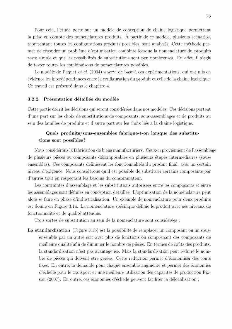
alors se faire en phase d’industrialisation. Un exemple de nomenclature pour deux produits
est donne en Figure 3.1a. La nomenclature specifique definie le produit avec ses niveaux de
fonctionnalite et de qualite attendus.
Trois sortes de substitution au sein de la nomenclature sont considerees :
La standardisation (Figure 3.1b) est la possibilite de remplacer un composant ou un sous-
ensemble par un autre soit avec plus de fonctions ou comprenant des composants de
meilleure qualite afin de diminuer le nombre de pieces. En termes de couts des produits,
la standardisation n’est pas avantageuse. Mais la standardisation peut reduire le nom-
bre de pieces qui doivent etre gerees. Cette reduction permet d’economiser des couts
fixes. En outre, la demande pour chaque ensemble augmente et permet des economies
d’echelle pour le transport et une meilleure utilisation des capacites de production Fix-
son (2007). En outre, ces economies d’echelle peuvent faciliter la delocalisation ;
24
(a) Nomenclatures speci-fiques
(b) Standardisation
(c) Gamme d’assemblage alternative
Figure 3.1 Illustration de nomenclatures et des possibilites de substitution.
L’externalisation : un sous-ensemble peut etre achete directement a un sous-traitant au
lieu d’etre fabrique. L’externalisation permet de reduire les couts fixes de production
mais augmente les couts variables. Dans l’exemple de la Figure 3.1a, les sous-ensembles
A ou B pourrait etre achetes;
La gamme d’assemblage alternative (Figure 3.1c) : differentes facons d’assembler les
produits sont enumerees. Cela peut permettre une mise en commun des sous-ensembles
permettant de reduire la diversite en production. Les couts de production sont a priori
les memes.
Quel reseau logistique mettre en place pour produire et distribuer
les produits?
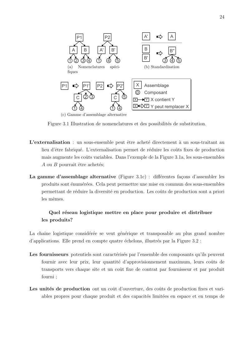
La chaıne logistique consideree se veut generique et transposable au plus grand nombre
d’applications. Elle prend en compte quatre echelons, illustres par la Figure 3.2 :
Les fournisseurs potentiels sont caracterises par l’ensemble des composants qu’ils peuvent
fournir avec leur prix, leur quantite d’approvisionnement maximum, leurs couts de
transports vers chaque site et un cout fixe de contrat par fournisseur et par produit
fourni ;
Les unites de production ont un cout d’ouverture, des couts de production fixes et vari-
ables propres pour chaque produit et des capacites limitees en espace et en temps de
25
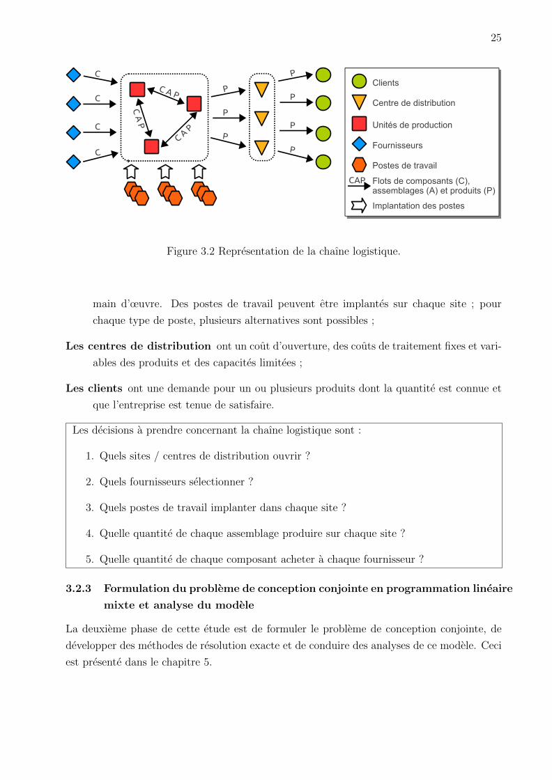
Figure 3.2 Representation de la chaıne logistique.
main d’œuvre. Des postes de travail peuvent etre implantes sur chaque site ; pour
chaque type de poste, plusieurs alternatives sont possibles ;
Les centres de distribution ont un cout d’ouverture, des couts de traitement fixes et vari-
ables des produits et des capacites limitees ;
Les clients ont une demande pour un ou plusieurs produits dont la quantite est connue et
que l’entreprise est tenue de satisfaire.
Les decisions a prendre concernant la chaıne logistique sont :
1. Quels sites / centres de distribution ouvrir ?
2. Quels fournisseurs selectionner ?
3. Quels postes de travail implanter dans chaque site ?
4. Quelle quantite de chaque assemblage produire sur chaque site ?
5. Quelle quantite de chaque composant acheter a chaque fournisseur ?
3.2.3 Formulation du probleme de conception conjointe en programmation lineaire
mixte et analyse du modele
La deuxieme phase de cette etude est de formuler le probleme de conception conjointe, de
developper des methodes de resolution exacte et de conduire des analyses de ce modele. Ceci
est presente dans le chapitre 5.
26
Modelisation La programmation lineaire mixte a ete retenue pour la modelisation car son
utilisation tres repandue a montre de tres bons resultats pour ce type de probleme.
Le modele de base reste celui de Paquet et al. (2004) car celui-ci couvre une grande
partie de notre champs d’application concernant la chaıne logistique. Des modifications
mineures sont apportees a ce modele, telles que la prise en compte des centres de
distribution et l’ajout de couts fixes concernant la gestion des produits et des transports.
L’apport majeur au niveau de la modelisation reside dans l’integration des possibil-
ites de substitution. La difficulte est de garder un modele lineaire, tout en limitant la
complexite de la formulation. Le modele utilise par Chen (2010) demontre bien la com-
plexite de cette formulation dans un cadre general : les variables de decision formulant
les substitutions sont tres nombreuses.
La section 5.2.2 presente notre formulation, qui integre les susbstitutions dans les con-
traintes de flots mais en les decouplant des variables modelisant la production – a
l’inverse du modele de Chen qui lie ces variables. Les premiers resultats montrent que
cette formulation ne complexifie pas la resolution lorsque l’algorithme de branch-and-
bound de Cplex est utilise.
Methodes de resolution exactes Les puissances de calcul actuelles couplees a des solveurs
performants (les librairies Java de Cplex 12 d’Ilog-IBM sont utilisees) permettent de
resoudre des instances de tailles raisonnables – de l’ordre de 30 fournisseurs, 10 sites,
10 postes de travail, 20 produits avec une centaine d’assemblages et de composants.
Cependant, la resolution est fortement influencee par la configuration des instances,
notamment le rapport entre les couts fixes et variables. Des methodes de resolution
exacte doivent etre developpees pour rendre la resolution plus robuste et permettre de
traiter de plus grosses instances.
L’etude de la litterature fait apparaıtre les benefices de la decomposition de Benders
ainsi que l’ajout d’inegalites valides. Ce sont nos pistes de travail.
Experimentation Le modele propose peut etre etudie d’un point de vue experimental, en
testant des instances representatives de plusieurs types de situations reelles. En parti-
culier, il sera interessant d’analyser dans quelles conditions les possibilites de substitu-
tion apportent des benefices. L’equilibre entre les surcouts de substitution et les couts
d’implantation joue a priori un role important. Le degre de commonalite d’une famille
de produit et les conditions du marche doivent egalement influencer les decisions. Enfin,
un interet particulier sera porte aux strategies mises en place pour rendre la chaıne lo-
gistique plus robuste comme le multi-sourcing, ainsi qu’aux contraintes sociales comme
27
garantir un niveau d’activite sur un site.
Nos donnees industrielles ne permettent pas de construire des cas d’etudes d’assez
grandes envergures. Ces experimentations porteront donc sur des instances academiques.
Pour cela, un generateur d’instances a ete developpe, notamment pour construire des
nomenclatures d’une famille de produits en controlant son niveau de commonalite.
3.2.4 Developpement d’un outil d’aide a la decision
Le developpement d’un outil d’aide a la decision necessite de penser a l’utilisation sur le
terrain des donnees et des resultats. Les besoins sont alors differents de ce qu’apporte le
modele d’optimisation decrit ci-avant. Les trois aspects suivants sont indispensables pour un
outil d’aide a la decision :
Determiner les parametres pertinents Les parametres d’entree du modele d’optimisation
ne sont pas disponibles en l’etat sur le terrain. Un traitement des donnees reelles est
donc indispensable. Pour cela, il faut determiner les donnees a recueillir sur le terrain et
comment les agreger et les modifier en gardant tout le sens du probleme. Les parametres
les plus difficiles a evaluer sont les couts de gestion des produits. Un autre question-
nement est le niveau de detail a donner au modele. Faut-il retranscrire fidelement la
realite ou decider du niveau d’agregation le plus pertinent ?
Donner des solutions rapidement Avec des donnees parfaites, il est envisageable de dis-
poser d’un temps de calcul raisonnable avant de donner une solution. Malheureusement,
de telles donnees n’existent pas et les decideurs ont besoin de reagir face aux resultats.
Les donnees peuvent etre ajustees plusieurs fois pour verifier l’impact que peut avoir
une variation non prevue, ou forcer une partie de la solution pour obtenir des resultats
plus coherent. Pour permettre de telles interactions avec l’outil, le temps de resolution
doit etre court – de l’ordre de la seconde si l’on souhaite des interactions graphiques ou
au pire de la minute.
Des heuristiques et des meta-heuristiques doivent donc etre developpees pour obtenir
de bonnes solutions en un temps tres court.
Representer des resultats permettant de prendre une decision Le cout ne peut pas
etre le seul critere de choix. Une solution parfaite au niveau mathematique contient
toutes les simplifications de modelisation qui ont permis de retranscrire la realite. Ainsi,
seul le jugement du decideur est valide, car celui-ci peut analyser la pertinence de la
solution. Pour cela, il faut representer les solutions de maniere a ce qu’elles puissent etre
analysables facilement. Les outils a notre disposition sont les resultats chiffres, a mettre
28
en perspectives par des ratios et des graphiques, des representations geographiques des
sites et des flux... Les indicateurs pertinents doivent etre determines.
L’outil developpe est presente en annexe A. Il n’integre pas les aspects environnementaux.
3.3 Contributions
Nous nous sommes interesses aux liens entre l’optimisation des familles de produits et de la
chaıne logistique. Tout d’abord, pour analyser les mecanismes des deux processus et leurs
interdependances, la standardisation dans le contexte de la delocalisation a ete etudiee Baud-
Lavigne et al. (2010). Une etude plus generale a ete publiee Baud-Lavigne et al. (2012b), voir
Chapitre 4, qui justifie l’utilisation de methodes d’optimisation conjointe. Dans cet article,
nous nous interessons plus precisement aux liens entre la standardisation des produits ou
des composants, et la conception de la chaıne logistique. Tout d’abord, nous montrons sur
un petit exemple qu’il peut exister un grand interet a considerer simultanement ces deux
decisions, et que la resolution de ces problemes separement pourrait aboutir a une decision
sous-optimale. Puis, sur un probleme simplifie provenant d’une etude de cas industrielle,
nous decrivons l’impact des choix de standardisation sur la structure de la chaıne logistique
et le gain qui peut etre obtenu par une resolution conjointe des problemes. Pour illustrer
les solutions du probleme, nous proposons des graphiques afin de visualiser, en fonction des
quantites et / ou des couts de transport, la meilleure decision pour la standardisation des
produits et de la conception de la chaıne logistique. Ces graphiques permettent egalement
d’anticiper les impacts d’une variation soit de quantite ou des couts de transport, d’une sit-
uation specifique. De tels graphiques peuvent etre utilises dans un outil d’aide a la decision
pour guider les entreprises dans leurs choix. Enfin, nous montrons que les couts et la struc-
ture de la chaıne logistique sont tres touchees par ces decisions.
Un modele de conception conjointe de produits et de la chaıne logistique a ete presente
Baud-Lavigne et al. (2011b), avec pour avantages que l’ajout des substitutions n’impacte pas
fortement les temps de resolution. Les problematiques multi-sourcing et de niveau d’activite
minimale sur le meme modele ont ete etudiees Baud-Lavigne et al. (2011a). Enfin, une etude
des temps et des methodes de resolution, ainsi qu’un generateur d’instance complexe a ete
propose Baud-Lavigne et al. (2012c), voir Chapitre 5. Nous presentons dans cet article un
modele general qui prend en compte simultanement la construction de la nomenclature et
de la conception du reseau logistique. Pour la nomenclature, des possibilites de substitution
des produits, sous-ensembles et composants sont prises en compte. Pour le reseau logistique,
les sites de production et la localisation des centres de distribution sont consideres ainsi que
le choix des fournisseurs. Un programme lineaire en variables mixtes (PLNE) est propose.
29
La formulation PLNE est resolue de maniere optimale pour les instances de taille moyenne.
Pour les instances de taille plus grande, deux heuristiques derivees du PLNE sont concues.
Ces methodes sont testees sur des instances de natures et de tailles differentes a partir d’un
generateur concu a cet effet.
Une revue de la litterature sur les liens entre la conception de familles de produits et des
reseaux logistiques a fait l’objet d’une conference Baud-Lavigne et al. (2011c).
La derniere contribution concerne l’integration de contraintes environnementales Baud-Lavigne
et al. (2012a), voir Chapitre 6. Il s’agit d’une extension des travaux presentes dans le
Chapitre 5. Les preoccupations environnementales commencent a etre prises en compte par
les industriels, du fait des contraintes legales et des preferences des consommateurs. Nous
proposons d’integrer ces contraintes dans la conception des familles de produits et de leur
chaıne logistique. Un modele mathematique est propose pour optimiser les couts en lim-
itant les emissions carbones, un autre permettant d’optimiser les emissions carbones sous
contrainte de cout limite. L’impact de ces contraintes est analyse en les resserrant plus ou
moins. Globalement, des resultats de qualite acceptable peuvent etre obtenus lorsque les
contraintes ne sont pas trop resserrees.

30
31
PARTIE II
CONTRIBUTIONS

33
CHAPITRE 4
MUTUAL IMPACTS OF PRODUCT STANDARDIZATION AND SUPPLY
CHAIN DESIGN
Abstract 1 : This paper deals with two major issues for industries: the product design and
the supply chain design. These problems are usually solved separately, but in recent years,
approaches were proposed to tackle these two problems together. In this paper, we investigate
more precisely the links between the standardization of products or components, and the
design of the supply chain. First, we show on a little example that there is a great interest to
consider simultaneously these two decisions, and that solving these interdependent problems
separately could result in a suboptimal, or even a bad decision. Then, on a simplified problem
issued from an industrial case study, we outline the impact of standardization choices on the
structure of the supply chain and the gain that can be obtained from solving the problem
as a unique compound optimization model. To illustrate the solutions of the problem, we
propose graphics in order to visualize, in function of quantities and/or transportation costs,
the best decision for the product standardization and for the supply chain design. Graphics
also permit to anticipate the impacts of a variation of either quantities or transportation
costs, from a specific situation. Such graphics they could be used in a decision aid tool to
help companies in their choices. Finally, we show that costs and supply chain structure are
highly impacted.
Keywords: Supply chain design, Product standardization, Relocation cost, Mixed Integer
Linear Programming
4.1 Introduction
In a highly competitive business environment, companies must diversify their offers to meet
customer’s demands. Managing diversity is a central issue: how to offer a wide variety of
products that meet customer’s needs, while controlling production, inventory and logistical
costs? The answers usually involve many separate disciplines, mainly product design, pro-
duction and logistics. Interdisciplinary, however, appears as a key in managing diversity
(Riopel et al. (1998)).
Integrating product and supply chain optimization is facing two important barriers. The
1 Baud-Lavigne, B., Agard, B. et Penz, B., 2012. Mutual impacts of product standardization and supplychain design. International Journal of Production Economics, 135(1) : 50-60.
34
first issue is to prove that the simultaneous design of the product and the supply chain is
relevant. In fact, cost from the product itself should be much higher than logistical and
production costs. Appelqvist et al. (2004) explain this in a recent survey:
“ Why is there then a lack of research into modelling of supply chains in the
product design phase? Perhaps, in the final analysis, it is not important. Material
costs typically stand for the majority of the product costs, and are determined in
the product design phase. If these, in turn, are determined by the desired product
functionality, there is little that supply chain modelling can achieve. ”
However, this limitation is slowly taking down with the increase of transportation costs
mainly due to oil price and carbon taxes. Also, simultaneous optimization of criteria is rel-
evant if and only if there exist linked impacts between these criteria. Otherwise, sequential
optimization can be used. It is well established that product design has a great impact on
manufacturing and logistics (Dowlatshahi (1996)). However, the opposite link has to be high-
lighted. This paper focuses on this first issue.
The second issue concerns the solution of such a combined problem. The integrated
supply chain design is already a complex problem. Adding new decisions, such as product
standardization, increases the difficulty to model the problem and to solve it efficiently.
When considering mass customization, it may be sub-optimal to first design the product,
and then the supply chain. A review of the current literature shows that attention is mainly
given on separated approaches, while very few studies consider joint design. Nevertheless,
joint design of product standardization and supply chain offers new perspectives. Standard-
ization is the possibility of replacing a component or a sub-assembly by another one with
either more function or including components with higher quality in order to decrease the
number of parts. In terms of product costs, the standardization is not advantageous. However
standardization can reduce the number of parts that have to be managed. This reduction
permits to save fixed costs. Furthermore, the demand for each part increases economies of
scale for transportation and permits a better use of production capacity (Fixson (2007)). This
can provide economies of scale to allow cheaper relocation. To highlight this, a little case
study is proposed to show the optimality of the joint design on sequential design under some
restrictive hypotheses. Then, the analysis of more realistic cases shows various impacts of the
standardization on the supply chain design. To illustrate the solutions of the problem, we
propose graphics in order to visualize, in function of quantities and/or transportation costs,
the best decision for the product standardization and for the supply chain design. Graphics
35
also permit to anticipate the impacts of a variation of either quantities or transportation
costs, from a specific situation. Such graphics could be used in a decision aid tool to help
companies in their choices. Finally, we show that costs and supply chain structure are highly
impacted.
The paper is organized as follows. In Section 4.2, a literature review is given. Section 4.3,
presents the problem of supply chain design considering product standardization. A small
example shows that, in certain circumstances, product standardization and product alloca-
tion must be taken into account simultaneously. To better understand the links between
product standardization and the supply chain, numerical experiments are led using MILP
exact solution (Section 4.4). These results show that the impacts are important for both
costs and structure of the solutions. Section 4.5 concludes the paper and proposes ways to
investigate this difficult problem.
4.2 Literature review on product and supply chain design
In product design, high diversity at low cost can be obtained through mass customization,
concept well defined by Pine (1993). Mass customization seeks to offer a wide variety of
finished product with the advantages of mass production, i.e. low production, storage and
logistic costs. Mass customization involves a set of concepts that can be used at the prod-
uct design stage: modular design, scalability and commonality. Modular design (Kusiak et
Huang (1996)) consists to assemble the product from functional modules. Scalability al-
lows easy changes to the product, while, commonality (Fixson (2007)) reuses components or
sub-assemblies of other existing products. During the industrialization phase, delayed dif-
ferentiation (Su et al. (2005)) has permitted to personalize products in the manufacturing
process (Fournier et Agard (2007)). These developments offered new opportunities for opti-
mization. Authors then worked on either optimization of product families to meet customer
needs precisely and at lowest cost (Briant et Naddef (2004) Barajas et Agard (2009)) or
module optimization (da Cunha et al. (2007) Agard et Penz (2009)).
Once the product is designed, the goal is then to reduce logistic costs by the design of a
supply chain, taking into account both strategical and tactical decisions. The strategic level
includes decisions impacting the long term of the company. For example the choice of produc-
tion facilities, their load / manufacturing capacities and technologies used may be viewed as
strategic. The tactical level includes mid-term decisions, such as the choice of suppliers, the
allocation of products to production facilities, and the flow of each product and sub-assembly
36
in the network (Cordeau et al. (2006)). The parameters considered in the supply chain design
problem are related to the manufacturing (cost structure, workforce, capacity etc.) and to
the logistics induced by a dispersion of production sites. Many studies have focused on the
supply chain design problem, an overview is proposed by Shapiro (2001) who provided models
for a wide variety of issues related to supply chain. See also Melo et al. (2009) for the most
recent review for deterministic models and Peidro et al. (2009) for the stochastic models. A
comprehensive study on the logistical decisions is also proposed by Riopel et al. (2005) who
presented a framework which highlights all the links between the product and supply chain
design.
Joint product and supply chain design opens new perspectives in the issue of high di-
versity of products. Most approaches developed to solve this combined problem are crossed
approaches. The first type of approach consists to incorporate product constraints in the
supply chain design, by taking into account, for example, the assembly constraints. Inte-
grated supply chain models considering bill-of-materials are recent and still little studied.
Several single-period, multi-product and multi-level models have been proposed by Paquet
et al. (2004), Paquet et al. (2008), and Cordeau et al. (2006) and a multi-period model was
presented by Thanh et al. (2008). Some studies analyzed the impact of the product design
on the supply chain. For example, Salvador et al. (2004) investigated the consequences of the
level of mass-customization on the supply chain by an empirical research and showed that the
degree of customization has a significant impact on the supply chain configuration. Montreuil
et Poulin (2005) proposed a supply chain design suited to personalized manufacturing.
The second type of crossed approach is to integrate logistic constraints in the product de-
sign. Benefits of “ Design for Logistics ” (DFL) have been highlighted by Dowlatshahi (1996).
These approaches promote the use of concepts such as modular design, delayed differentiation
and other qualitative rules. Such as reducing the number of components or references used,
and integrating of upstream suppliers of design projects to allow lower costs associated with
storage and transportation products.
Integrated approaches, which involve complex models, are poorly investigated yet. The
simultaneous optimization of product and supply chain design is a difficult problem. Authors
have looked at partial models, simpler to solve and to implement. Gupta et Krishnan (1999)
presented a mixed integer programming formulation to integrate component standardization
and supplier selection decisions. Fixed and variable costs are associated to each different
component. The optimal solution is found with the proper level of standardization, which
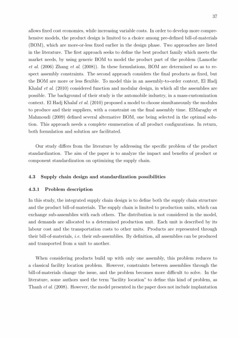
37
allows fixed cost economies, while increasing variable costs. In order to develop more compre-
hensive models, the product design is limited to a choice among pre-defined bill-of-materials
(BOM), which are more-or-less fixed earlier in the design phase. Two approaches are listed
in the literature. The first approach seeks to define the best product family which meets the
market needs, by using generic BOM to model the product part of the problem (Lamothe
et al. (2006) Zhang et al. (2008)). In these formulations, BOM are determined so as to re-
spect assembly constraints. The second approach considers the final products as fixed, but
the BOM are more or less flexible. To model this in an assembly-to-order context, El Hadj
Khalaf et al. (2010) considered function and modular design, in which all the assemblies are
possible. The background of their study is the automobile industry, in a mass-customization
context. El Hadj Khalaf et al. (2010) proposed a model to choose simultaneously the modules
to produce and their suppliers, with a constraint on the final assembly time. ElMaraghy et
Mahmoudi (2009) defined several alternative BOM, one being selected in the optimal solu-
tion. This approach needs a complete enumeration of all product configurations. In return,
both formulation and solution are facilitated.
Our study differs from the literature by addressing the specific problem of the product
standardization. The aim of the paper is to analyze the impact and benefits of product or
component standardization on optimizing the supply chain.
4.3 Supply chain design and standardization possibilities
4.3.1 Problem description
In this study, the integrated supply chain design is to define both the supply chain structure
and the product bill-of-materials. The supply chain is limited to production units, which can
exchange sub-assemblies with each others. The distribution is not considered in the model,
and demands are allocated to a determined production unit. Each unit is described by its
labour cost and the transportation costs to other units. Products are represented through
their bill-of-materials, i.e. their sub-assemblies. By definition, all assemblies can be produced
and transported from a unit to another.
When considering products build up with only one assembly, this problem reduces to
a classical facility location problem. However, constraints between assemblies through the
bill-of-materials change the issue, and the problem becomes more difficult to solve. In the
literature, some authors used the term ”facility location” to define this kind of problem, as
Thanh et al. (2008). However, the model presented in the paper does not include implantation
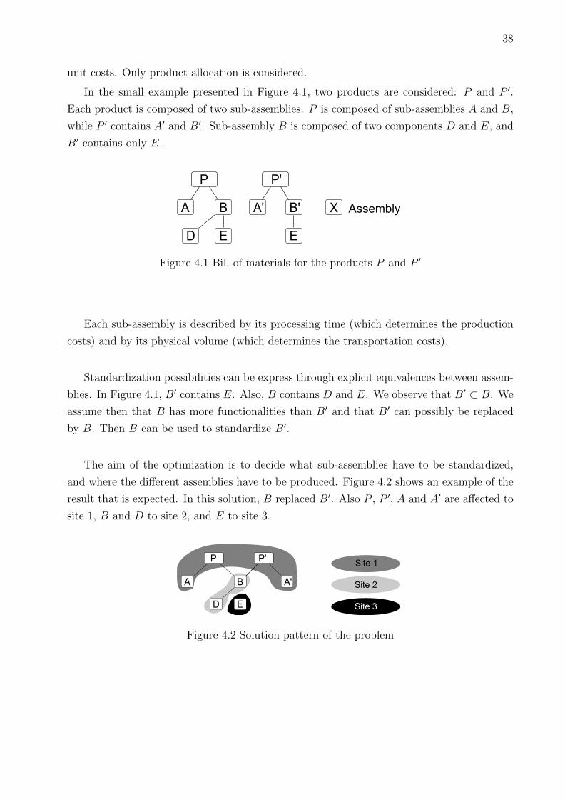
38
unit costs. Only product allocation is considered.
In the small example presented in Figure 4.1, two products are considered: P and P ′.
Each product is composed of two sub-assemblies. P is composed of sub-assemblies A and B,
while P ′ contains A′ and B′. Sub-assembly B is composed of two components D and E, and
B′ contains only E.
P
A B
D E
P'
A' B'
E
X Assembly
Figure 4.1 Bill-of-materials for the products P and P ′
Each sub-assembly is described by its processing time (which determines the production
costs) and by its physical volume (which determines the transportation costs).
Standardization possibilities can be express through explicit equivalences between assem-
blies. In Figure 4.1, B′ contains E. Also, B contains D and E. We observe that B′ ⊂ B. We
assume then that B has more functionalities than B′ and that B′ can possibly be replaced
by B. Then B can be used to standardize B′.
The aim of the optimization is to decide what sub-assemblies have to be standardized,
and where the different assemblies have to be produced. Figure 4.2 shows an example of the
result that is expected. In this solution, B replaced B′. Also P , P ′, A and A′ are affected to
site 1, B and D to site 2, and E to site 3.
Site 1
Site 2
Site 3
P
A B
D E
P'
A'
Figure 4.2 Solution pattern of the problem
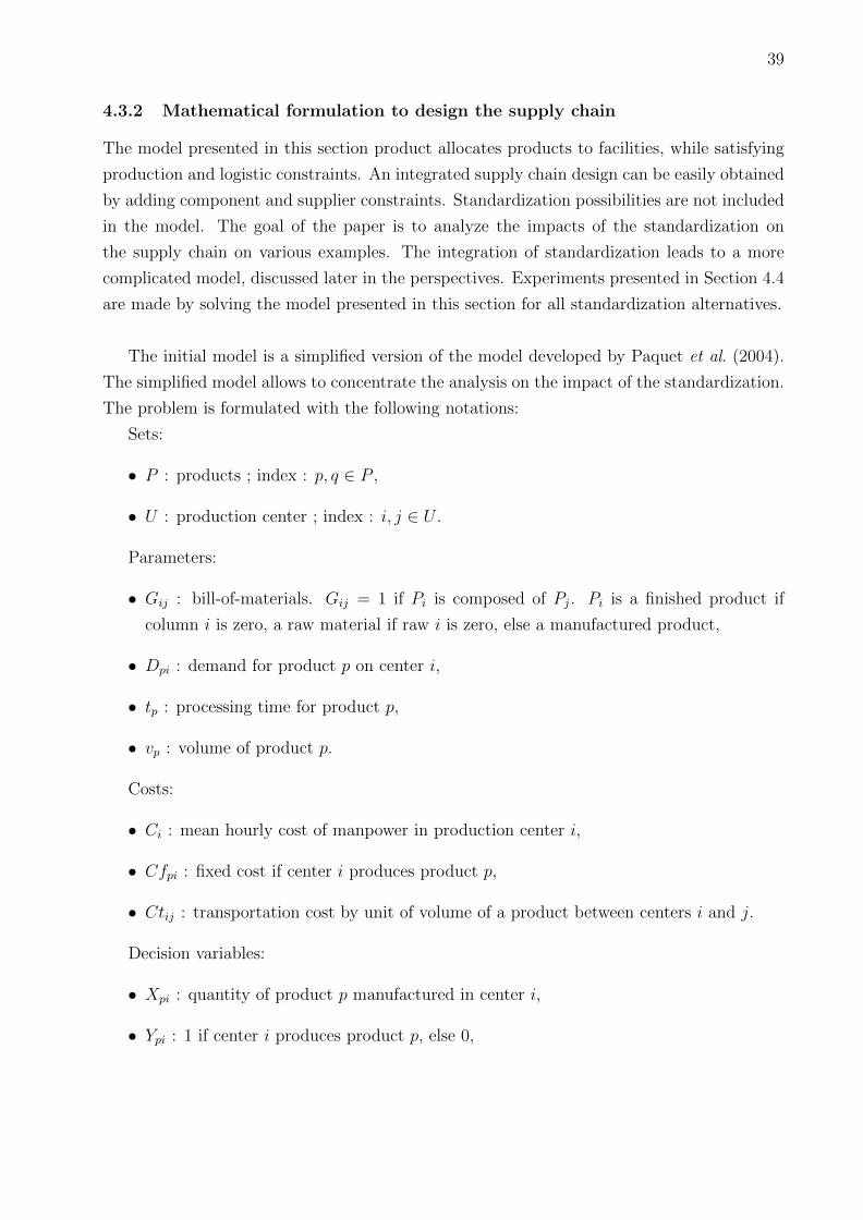
39
4.3.2 Mathematical formulation to design the supply chain
The model presented in this section product allocates products to facilities, while satisfying
production and logistic constraints. An integrated supply chain design can be easily obtained
by adding component and supplier constraints. Standardization possibilities are not included
in the model. The goal of the paper is to analyze the impacts of the standardization on
the supply chain on various examples. The integration of standardization leads to a more
complicated model, discussed later in the perspectives. Experiments presented in Section 4.4
are made by solving the model presented in this section for all standardization alternatives.
The initial model is a simplified version of the model developed by Paquet et al. (2004).
The simplified model allows to concentrate the analysis on the impact of the standardization.
The problem is formulated with the following notations:
Sets:
• P : products ; index : p, q ∈ P ,
• U : production center ; index : i, j ∈ U .
Parameters:
• Gij : bill-of-materials. Gij = 1 if Pi is composed of Pj. Pi is a finished product if
column i is zero, a raw material if raw i is zero, else a manufactured product,
• Dpi : demand for product p on center i,
• tp : processing time for product p,
• vp : volume of product p.
Costs:
• Ci : mean hourly cost of manpower in production center i,
• Cfpi : fixed cost if center i produces product p,
• Ctij : transportation cost by unit of volume of a product between centers i and j.
Decision variables:
• Xpi : quantity of product p manufactured in center i,
• Ypi : 1 if center i produces product p, else 0,
40
• Fpij : flow of product p from center i to center j.
Then, the supply chain design problem can be formulated as a Mixed Integer Linear
Program as follows:
Z = min∑i∈U
∑p∈P
(XpiCitp + YpiCfpi) +∑i∈U
∑j∈U\i
∑p∈P
FpijCtijvp (4.1)
s.t.
Xpi +∑j∈U\i
Fpji =∑j∈U\i
Fpij +∑q∈P\p
GqpXqi +Dpi ∀i ∈ U,∀p ∈ P (4.2)
Xpi ≤ YpiDp ∀i ∈ U,∀p ∈ P (4.3)
Xpi ∈ Z+ ∀i ∈ U,∀p ∈ P (4.4)
Ypi ∈ {0, 1} ∀i ∈ U,∀p ∈ P (4.5)
Fpij ∈ Z+ ∀i, j ∈ U,∀p ∈ P (4.6)
The objective function (1) minimizes production and transportation costs. Constraints
(4.2) are the flow constraints, described in Figure 4.3. For each product p on a center i,
entering flows represent products transported from every other centers to i, and production
of p on i (the source), while outgoing flows represent products p transported from i to every
other centers, products in the bills-of-materials of other assemblies produced in i and the
demand (the sink). Constraints (4.3) assure that fixed costs are paid when a product is
manufactured on a unit. When Xpi > 0, Ypi = 1. To verify this inequality, Dp must be a
constant greater that Xpi. So, Dp is the total demand associated with assembly p in the
whole supply chain. Constraints (4.4), (4.5) and (4.6) define decision variables as positive
integers for X and F , and as boolean for Y .
j i
Fpji
Fpij
GqpXqi
Xpi
dpi
Figure 4.3 Flow of assembly p on site i
4.3.3 Relevance of joint standardization and supply chain optimization
The following example is a small case built to show that standardization and supply chain
design should be tackled simultaneously. In this small case, we look for a situation in which
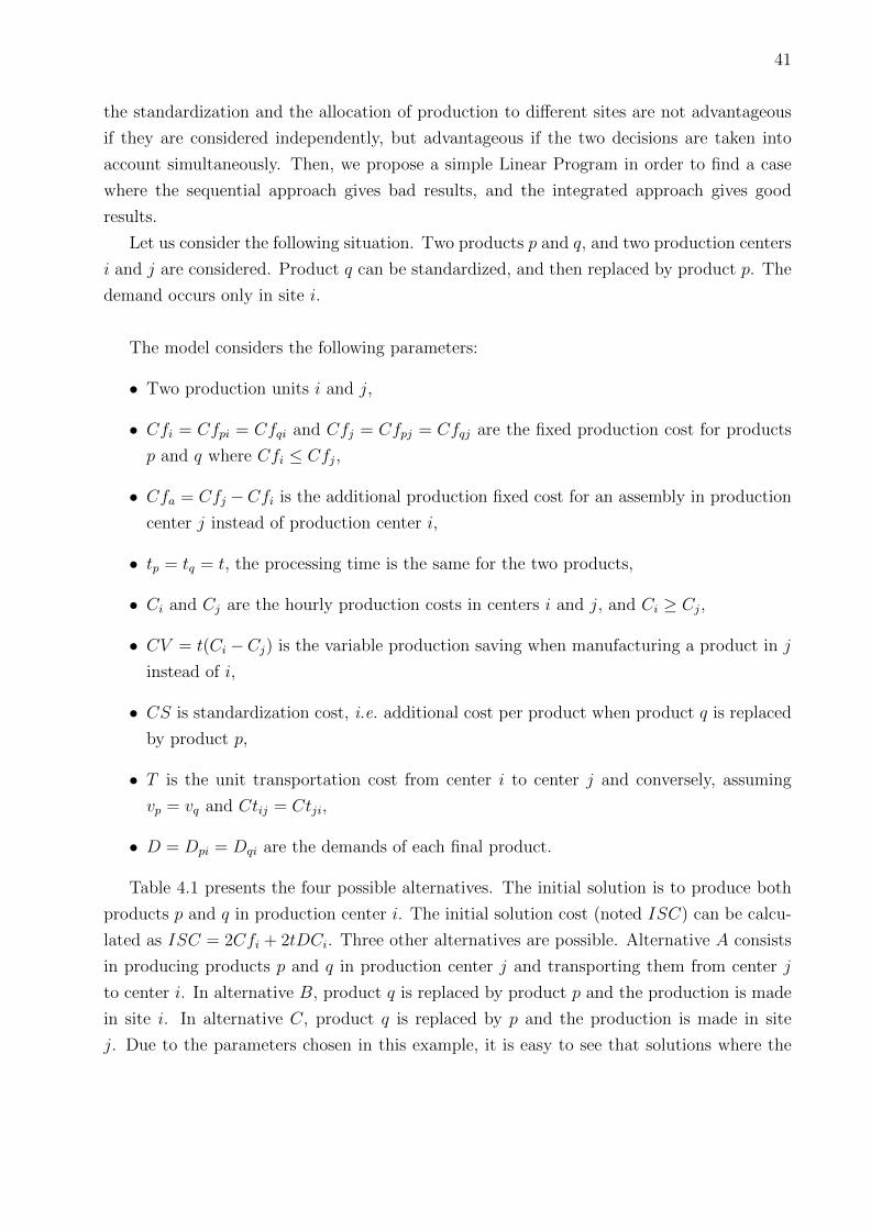
41
the standardization and the allocation of production to different sites are not advantageous
if they are considered independently, but advantageous if the two decisions are taken into
account simultaneously. Then, we propose a simple Linear Program in order to find a case
where the sequential approach gives bad results, and the integrated approach gives good
results.
Let us consider the following situation. Two products p and q, and two production centers
i and j are considered. Product q can be standardized, and then replaced by product p. The
demand occurs only in site i.
The model considers the following parameters:
• Two production units i and j,
• Cfi = Cfpi = Cfqi and Cfj = Cfpj = Cfqj are the fixed production cost for products
p and q where Cfi ≤ Cfj,
• Cfa = Cfj −Cfi is the additional production fixed cost for an assembly in production
center j instead of production center i,
• tp = tq = t, the processing time is the same for the two products,
• Ci and Cj are the hourly production costs in centers i and j, and Ci ≥ Cj,
• CV = t(Ci −Cj) is the variable production saving when manufacturing a product in j
instead of i,
• CS is standardization cost, i.e. additional cost per product when product q is replaced
by product p,
• T is the unit transportation cost from center i to center j and conversely, assuming
vp = vq and Ctij = Ctji,
• D = Dpi = Dqi are the demands of each final product.
Table 4.1 presents the four possible alternatives. The initial solution is to produce both
products p and q in production center i. The initial solution cost (noted ISC) can be calcu-
lated as ISC = 2Cfi + 2tDCi. Three other alternatives are possible. Alternative A consists
in producing products p and q in production center j and transporting them from center j
to center i. In alternative B, product q is replaced by product p and the production is made
in site i. In alternative C, product q is replaced by p and the production is made in site
j. Due to the parameters chosen in this example, it is easy to see that solutions where the
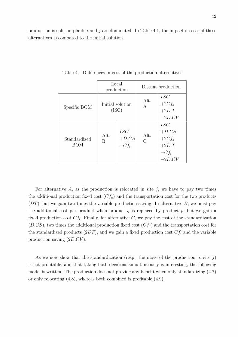
42
production is split on plants i and j are dominated. In Table 4.1, the impact on cost of these
alternatives is compared to the initial solution.
Table 4.1 Differences in cost of the production alternatives
Localproduction
Distant production
Specific BOMInitial solution
(ISC)
Alt.A
ISC
+2Cfa
+2D.T
−2D.CV
StandardizedBOM
Alt.B
ISC
+D.CS
−Cfi
Alt.C
ISC
+D.CS
+2Cfa
+2D.T
−Cfi−2D.CV
For alternative A, as the production is relocated in site j, we have to pay two times
the additional production fixed cost (Cfa) and the transportation cost for the two products
(DT ), but we gain two times the variable production saving. In alternative B, we must pay
the additional cost per product when product q is replaced by product p, but we gain a
fixed production cost Cfi. Finally, for alternative C, we pay the cost of the standardization
(D.CS), two times the additional production fixed cost (Cfa) and the transportation cost for
the standardized products (2DT ), and we gain a fixed production cost Cfi and the variable
production saving (2D.CV ).
As we now show that the standardization (resp. the move of the production to site j)
is not profitable, and that taking both decisions simultaneously is interesting, the following
model is written. The production does not provide any benefit when only standardizing (4.7)
or only relocating (4.8), whereas both combined is profitable (4.9).
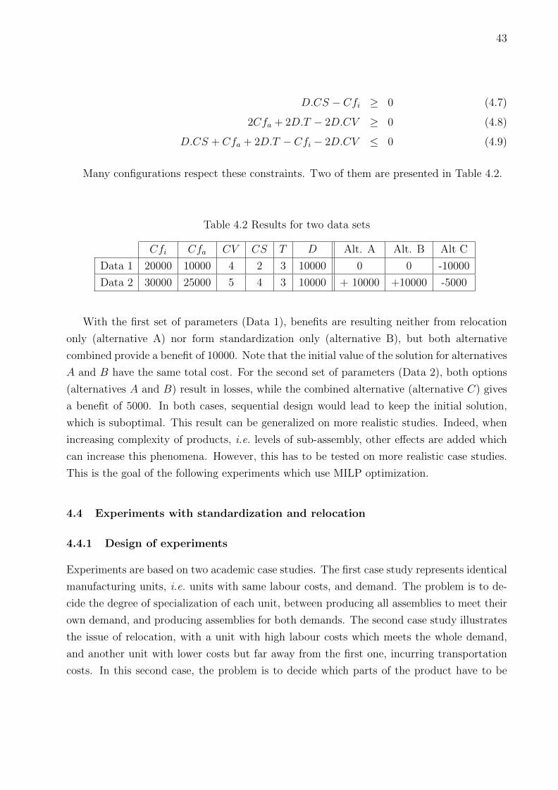
43
D.CS − Cfi ≥ 0 (4.7)
2Cfa + 2D.T − 2D.CV ≥ 0 (4.8)
D.CS + Cfa + 2D.T − Cfi − 2D.CV ≤ 0 (4.9)
Many configurations respect these constraints. Two of them are presented in Table 4.2.
Table 4.2 Results for two data sets
Cfi Cfa CV CS T D Alt. A Alt. B Alt C
Data 1 20000 10000 4 2 3 10000 0 0 -10000
Data 2 30000 25000 5 4 3 10000 + 10000 +10000 -5000
With the first set of parameters (Data 1), benefits are resulting neither from relocation
only (alternative A) nor form standardization only (alternative B), but both alternative
combined provide a benefit of 10000. Note that the initial value of the solution for alternatives
A and B have the same total cost. For the second set of parameters (Data 2), both options
(alternatives A and B) result in losses, while the combined alternative (alternative C) gives
a benefit of 5000. In both cases, sequential design would lead to keep the initial solution,
which is suboptimal. This result can be generalized on more realistic studies. Indeed, when
increasing complexity of products, i.e. levels of sub-assembly, other effects are added which
can increase this phenomena. However, this has to be tested on more realistic case studies.
This is the goal of the following experiments which use MILP optimization.
4.4 Experiments with standardization and relocation
4.4.1 Design of experiments
Experiments are based on two academic case studies. The first case study represents identical
manufacturing units, i.e. units with same labour costs, and demand. The problem is to de-
cide the degree of specialization of each unit, between producing all assemblies to meet their
own demand, and producing assemblies for both demands. The second case study illustrates
the issue of relocation, with a unit with high labour costs which meets the whole demand,
and another unit with lower costs but far away from the first one, incurring transportation
costs. In this second case, the problem is to decide which parts of the product have to be
44
transferred to the distant unit.
In both cases, the products considered are illustrated in Figure 4.4 and their characteris-
tics are given in Table 4.3. Sub-assembly A is large, so costly in transportation, while B is
small, but using more processing time.
P
A B
D E
P'
A' B'
E
P
AB
D E
P'
B'
E
P
A B
D E
P'
A'
P
A B
D E
no standardization A standardization B standardization P standardization
Figure 4.4 Standardization possibilities
Table 4.3 Product characteristics
Sub-assemblies
P P ′ A A′ B B′ D E
Volume (in m3) 0.6 0.5 0.5 0.3 0.05 0.05 0.005 0.02
Processing time (in h) 1.7 1.5 0.5 0.45 0.4 0.3 0.2 0.2
The standardization possibilities for product P ′ are to substitute module A′ by A, or B′
by B, or the whole product P ′ by P . Additional costs of standardization are induced mainly
by volume increase for A, and processing time increase for B. When standardizing B, D
has to be produced for P ′, which adds processing time. Consequently, A standardization
is sensitive to transportation cost variation, while B′ standardization is sensitive to labour
cost, and P to both. Transportation costs are paid only when sub-assemblies are moved from
a unit to another. For a local production, A standardization has nearly no negative effect,
while B and P standardizations generate extra labour cost.
These case studies have been tested with the four standardization options, i.e. standard-
ization of A, B, P , or no standardization at all. Variations of parameters are presented in
Figure 4.4. For this case study, four models were solved. For a more general problem, this
number depends on the number of all possible standardization options and on the compat-
ibilities between them (this could be considered as different scenarios). In the worst case,
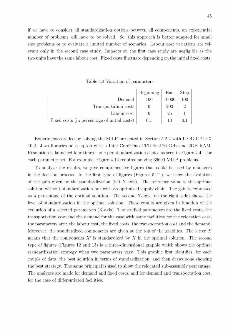
45
if we have to consider all standardization options between all components, an exponential
number of problems will have to be solved. So, this approach is better adapted for small
size problems or to evaluate a limited number of scenarios. Labour cost variations are rel-
evant only in the second case study. Impacts on the first case study are negligible as the
two units have the same labour cost. Fixed costs fluctuate depending on the initial fixed costs.
Table 4.4 Variation of parameters
Beginning End Step
Demand 100 10000 100
Transportation costs 0 200 2
Labour cost 0 25 1
Fixed costs (in percentage of initial costs) 0.1 10 0.1
Experiments are led by solving the MILP presented in Section 5.2.2 with ILOG CPLEX
10.2. Java libraries on a laptop with a Intel Core2Duo CPU @ 2.26 GHz and 2GB RAM.
Resolution is launched four times – one per standardization choice as seen in Figure 4.4 – for
each parameter set. For example, Figure 4.12 required solving 39600 MILP problems.
To analyze the results, we give comprehensive figures that could be used by managers
in the decision process. In the first type of figures (Figures 5–11), we show the evolution
of the gain given by the standardization (left Y-axis). The reference value is the optimal
solution without standardization but with an optimized supply chain. The gain is expressed
as a percentage of the optimal solution. The second Y-axis (on the right side) shows the
level of standardization in the optimal solution. These results are given in function of the
evolution of a selected parameters (X-axis). The studied parameters are the fixed costs, the
transportation cost and the demand for the case with same facilities; for the relocation case,
the parameters are : the labour cost, the fixed costs, the transportation cost and the demand.
Moreover, the standardized components are given at the top of the graphics. The letter X
means that the components X ′ is standardized by X in the optimal solution. The second
type of figures (Figures 12 and 13) is a three-dimensional graphic which shows the optimal
standardization strategy when two parameters vary. This graphic first identifies, for each
couple of data, the best solution in terms of standardization, and then draws zone showing
the best strategy. The same principal is used to show the relocated sub-assembly percentage.
The analyzes are made for demand and fixed costs, and for demand and transportation cost,
for the case of differentiated facilities.
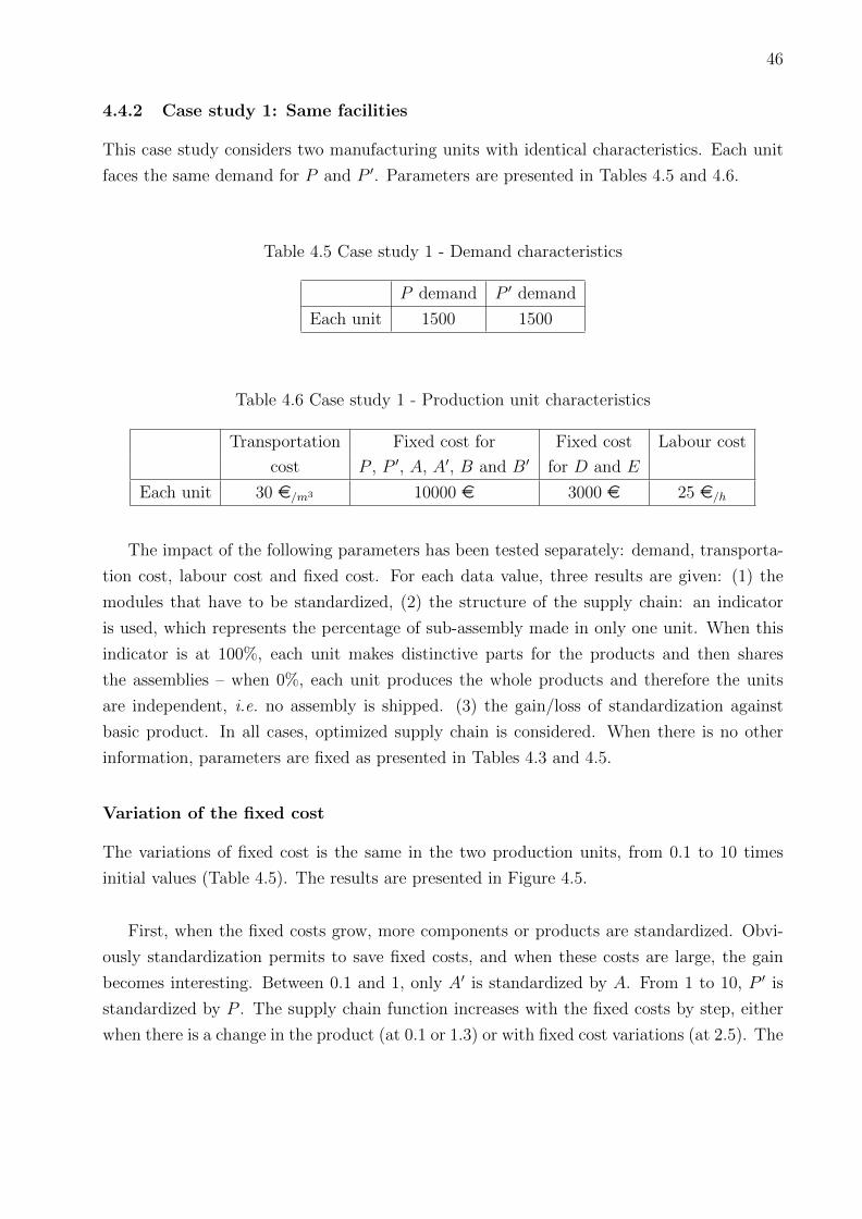
46
4.4.2 Case study 1: Same facilities
This case study considers two manufacturing units with identical characteristics. Each unit
faces the same demand for P and P ′. Parameters are presented in Tables 4.5 and 4.6.
Table 4.5 Case study 1 - Demand characteristics
P demand P ′ demand
Each unit 1500 1500
Table 4.6 Case study 1 - Production unit characteristics
Transportation Fixed cost for Fixed cost Labour cost
cost P , P ′, A, A′, B and B′ for D and E
Each unit 30 e/m3 10000 e 3000 e 25 e/h
The impact of the following parameters has been tested separately: demand, transporta-
tion cost, labour cost and fixed cost. For each data value, three results are given: (1) the
modules that have to be standardized, (2) the structure of the supply chain: an indicator
is used, which represents the percentage of sub-assembly made in only one unit. When this
indicator is at 100%, each unit makes distinctive parts for the products and then shares
the assemblies – when 0%, each unit produces the whole products and therefore the units
are independent, i.e. no assembly is shipped. (3) the gain/loss of standardization against
basic product. In all cases, optimized supply chain is considered. When there is no other
information, parameters are fixed as presented in Tables 4.3 and 4.5.
Variation of the fixed cost
The variations of fixed cost is the same in the two production units, from 0.1 to 10 times
initial values (Table 4.5). The results are presented in Figure 4.5.
First, when the fixed costs grow, more components or products are standardized. Obvi-
ously standardization permits to save fixed costs, and when these costs are large, the gain
becomes interesting. Between 0.1 and 1, only A′ is standardized by A. From 1 to 10, P ′ is
standardized by P . The supply chain function increases with the fixed costs by step, either
when there is a change in the product (at 0.1 or 1.3) or with fixed cost variations (at 2.5). The
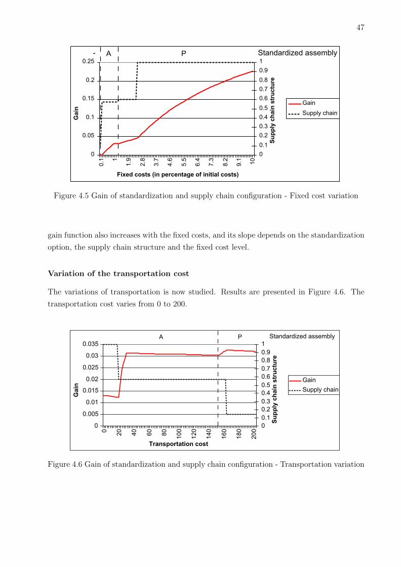
47
0
0.05
0.1
0.15
0.2
0.25
Fixed costs (in percentage of initial costs)
Ga
in
0
0.1
0.2
0.3
0.4
0.5
0.6
0.7
0.8
0.9
1
Su
pp
ly c
ha
in s
tru
ctu
re
Gain
Supply chain
Standardized assemblyA P-
0.1 1
1.9
2.8
3.7
4.6
5.5
6.4
7.3
8.2
9.1 10
Figure 4.5 Gain of standardization and supply chain configuration - Fixed cost variation
gain function also increases with the fixed costs, and its slope depends on the standardization
option, the supply chain structure and the fixed cost level.
Variation of the transportation cost
The variations of transportation is now studied. Results are presented in Figure 4.6. The
transportation cost varies from 0 to 200.
0
0.005
0.01
0.015
0.02
0.025
0.03
0.035
Transportation cost
Gain
0
0.1
0.2
0.3
0.4
0.5
0.6
0.7
0.8
0.9
1
Su
pp
ly c
hain
str
uc
ture
Gain
Supply chain
Standardized assemblyA P
0
20
40
60
80
10
0
12
0
14
0
16
0
18
0
20
0
Figure 4.6 Gain of standardization and supply chain configuration - Transportation variation
48
Predictable behaviours are highlighted. Shipped quantities decrease in two steps with
the increase of transportation costs. Below a transportation cost of 20, units are completely
specialized and A′ is standardized. Then, the product is the same but the supply chain design
changes: 40% of sub-assemblies are made in the two units. The gain increases rapidly from
1.25% to more than 3%. At 150, P ′ is standardized without any changes on the supply chain
design, but the gain increases of 0.25%. At 160, units become nearly independent, i.e. only
17% of modules are shared between the units.
Variation of the demand
The variations of demand is now studied. The demand is the same for each product at each
unit. Results are presented in Figure 4.7.
0
0.05
0.1
0.15
0.2
0.25
0.3
Demand
Ga
in
0
0.1
0.2
0.3
0.4
0.5
0.6
0.7
0.8
0.9
1
Su
pp
ly c
ha
in s
tru
ctu
reGain
Supply chain
Standardized assemblyAP B
10
0
10
00
19
00
28
00
37
00
46
00
55
00
64
00
73
00
82
00
91
00
10
00
0
Figure 4.7 Gain of standardization and supply chain configuration - Demand variation
As demand grows, sub-assemblies are less and less shared between the units. When the
demand is less than 800, the best solution is to standardize P ′. When demand varies between
800 and 8000, B′ is replaced by B. Afterwards, until the demand equals 10000, only A′ is
standardized. Also, when the demand varies from 100 to 10000, the gain falls dramatically
from 30% to 0%. When demand equals 500, the gain is of 5%, and drops down to 3% when
demand attains 1000.
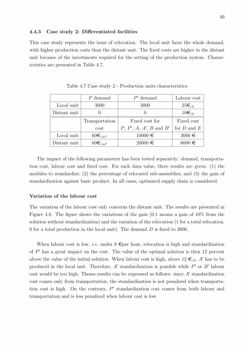
49
4.4.3 Case study 2: Differentiated facilities
This case study represents the issue of relocation. The local unit faces the whole demand,
with higher production costs than the distant unit. The fixed costs are higher in the distant
unit because of the investments required for the setting of the production system. Charac-
teristics are presented in Table 4.7.
Table 4.7 Case study 2 - Production units characteristics
P demand P ′ demand Labour cost
Local unit 3000 3000 25e/h
Distant unit 0 0 10e/h
Transportation Fixed cost for Fixed cost
cost P , P ′, A, A′, B and B′ for D and E
Local unit 60e/m3 10000 e 3000 e
Distant unit 60e/m3 20000 e 6000 e
The impact of the following parameters has been tested separately: demand, transporta-
tion cost, labour cost and fixed cost. For each data value, three results are given: (1) the
modules to standardize, (2) the percentage of relocated sub-assemblies, and (3) the gain of
standardization against basic product. In all cases, optimized supply chain is considered.
Variation of the labour cost
The variation of the labour cost only concerns the distant unit. The results are presented in
Figure 4.8. The figure shows the variations of the gain (0.1 means a gain of 10% from the
solution without standardization) and the variation of the relocation (1 for a total relocation,
0 for a total production in the local unit). The demand D is fixed to 3000.
When labour cost is low, i.e. under 8 eper hour, relocation is high and standardization
of P ′ has a great impact on the cost. The value of the optimal solution is then 12 percent
above the value of the initial solution. When labour cost is high, above 12 e/h, A′ has to be
produced in the local unit. Therefore, A′ standardization is possible while P ′ or B′ labour
cost would be too high. Theses results can be expressed as follows: since A′ standardization
cost comes only from transportation, the standardization is not penalized when transporta-
tion cost is high. On the contrary, P ′ standardization cost comes from both labour and
transportation and is less penalized when labour cost is low.
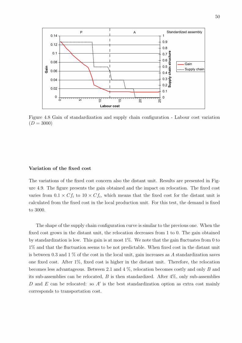
50
0
0.02
0.04
0.06
0.08
0.1
0.12
0.14
Labour cost
Gain
0
0.1
0.2
0.3
0.4
0.5
0.6
0.7
0.8
0.9
1
Su
pp
ly c
hain
str
uc
ture
Gain
Supply chain
Standardized assemblyAP
0 5
10
15
20
25
Figure 4.8 Gain of standardization and supply chain configuration - Labour cost variation(D = 3000)
Variation of the fixed cost
The variations of the fixed cost concern also the distant unit. Results are presented in Fig-
ure 4.9. The figure presents the gain obtained and the impact on relocation. The fixed cost
varies from 0.1 × Cfi to 10 × Cfi, which means that the fixed cost for the distant unit is
calculated from the fixed cost in the local production unit. For this test, the demand is fixed
to 3000.
The shape of the supply chain configuration curve is similar to the previous one. When the
fixed cost grows in the distant unit, the relocation decreases from 1 to 0. The gain obtained
by standardization is low. This gain is at most 1%. We note that the gain fluctuates from 0 to
1% and that the fluctuation seems to be not predictable. When fixed cost in the distant unit
is between 0.3 and 1 % of the cost in the local unit, gain increases as A standardization saves
one fixed cost. After 1%, fixed cost is higher in the distant unit. Therefore, the relocation
becomes less advantageous. Between 2.1 and 4 %, relocation becomes costly and only B and
its sub-assemblies can be relocated, B is then standardized. After 4%, only sub-assemblies
D and E can be relocated: so A′ is the best standardization option as extra cost mainly
corresponds to transportation cost.
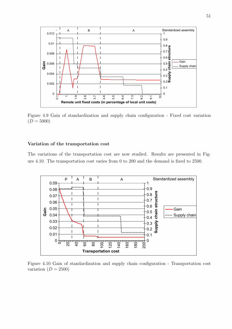
51
0
0.002
0.004
0.006
0.008
0.01
0.012
Remote unit fixed costs (in percentage of local unit costs)
Ga
in
0
0.1
0.2
0.3
0.4
0.5
0.6
0.7
0.8
0.9
1
Su
pp
ly c
ha
in s
tru
ctu
re
Gain
Supply chain
Standardized assemblyABA-
0.1 1
1.9
2.8
3.7
4.6
5.5
6.4
7.3
8.2
9.1 10
Figure 4.9 Gain of standardization and supply chain configuration - Fixed cost variation(D = 5000)
Variation of the transportation cost
The variations of the transportation cost are now studied. Results are presented in Fig-
ure 4.10. The transportation cost varies from 0 to 200 and the demand is fixed to 2500.
0
0.01
0.02
0.03
0.04
0.05
0.06
0.07
0.08
0.09
Transportation cost
Ga
in
0
0.1
0.2
0.3
0.4
0.5
0.6
0.7
0.8
0.9
1
Su
pp
ly c
ha
in s
tru
ctu
re
Gain
Supply chain
Standardized assemblyABP A
0
20
40
60
80
100
120
140
160
180
200
Figure 4.10 Gain of standardization and supply chain configuration - Transportation costvariation (D = 2500)
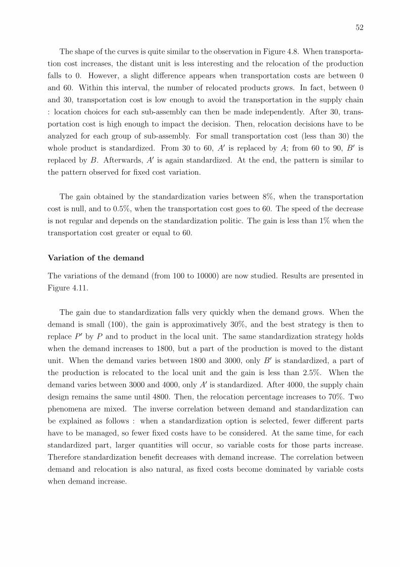
52
The shape of the curves is quite similar to the observation in Figure 4.8. When transporta-
tion cost increases, the distant unit is less interesting and the relocation of the production
falls to 0. However, a slight difference appears when transportation costs are between 0
and 60. Within this interval, the number of relocated products grows. In fact, between 0
and 30, transportation cost is low enough to avoid the transportation in the supply chain
: location choices for each sub-assembly can then be made independently. After 30, trans-
portation cost is high enough to impact the decision. Then, relocation decisions have to be
analyzed for each group of sub-assembly. For small transportation cost (less than 30) the
whole product is standardized. From 30 to 60, A′ is replaced by A; from 60 to 90, B′ is
replaced by B. Afterwards, A′ is again standardized. At the end, the pattern is similar to
the pattern observed for fixed cost variation.
The gain obtained by the standardization varies between 8%, when the transportation
cost is null, and to 0.5%, when the transportation cost goes to 60. The speed of the decrease
is not regular and depends on the standardization politic. The gain is less than 1% when the
transportation cost greater or equal to 60.
Variation of the demand
The variations of the demand (from 100 to 10000) are now studied. Results are presented in
Figure 4.11.
The gain due to standardization falls very quickly when the demand grows. When the
demand is small (100), the gain is approximatively 30%, and the best strategy is then to
replace P ′ by P and to product in the local unit. The same standardization strategy holds
when the demand increases to 1800, but a part of the production is moved to the distant
unit. When the demand varies between 1800 and 3000, only B′ is standardized, a part of
the production is relocated to the local unit and the gain is less than 2.5%. When the
demand varies between 3000 and 4000, only A′ is standardized. After 4000, the supply chain
design remains the same until 4800. Then, the relocation percentage increases to 70%. Two
phenomena are mixed. The inverse correlation between demand and standardization can
be explained as follows : when a standardization option is selected, fewer different parts
have to be managed, so fewer fixed costs have to be considered. At the same time, for each
standardized part, larger quantities will occur, so variable costs for those parts increase.
Therefore standardization benefit decreases with demand increase. The correlation between
demand and relocation is also natural, as fixed costs become dominated by variable costs
when demand increase.
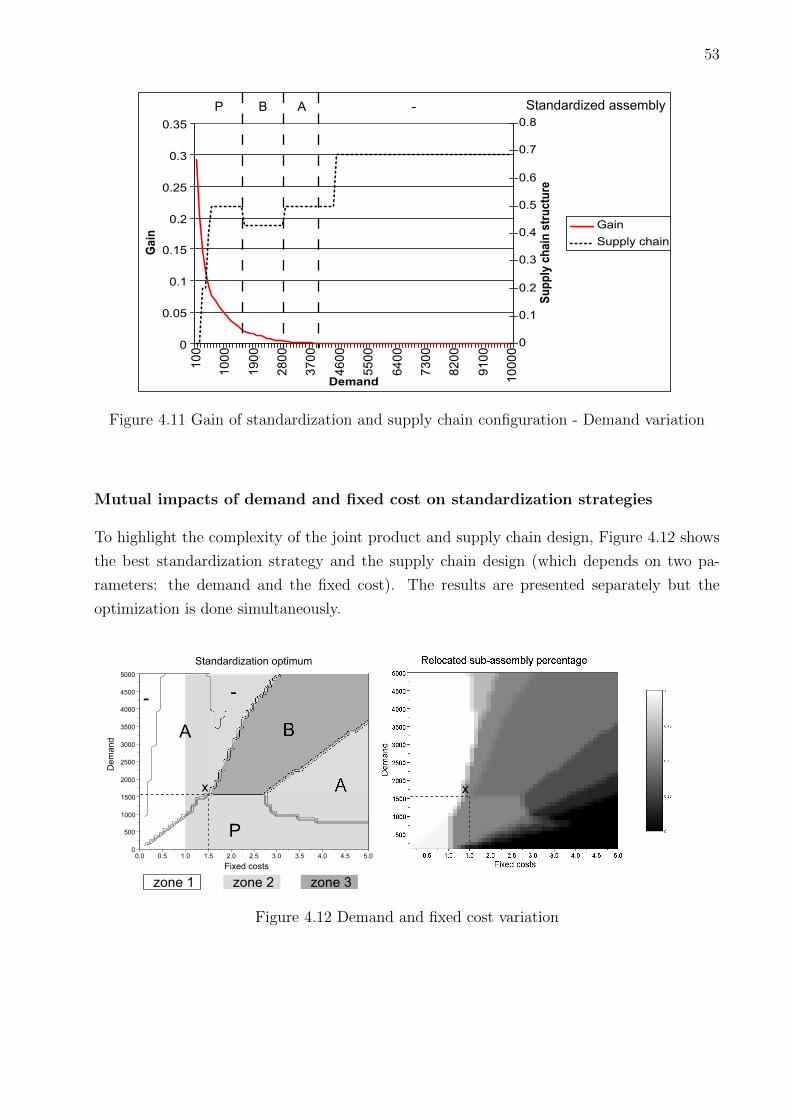
53
0
0.05
0.1
0.15
0.2
0.25
0.3
0.35
Demand
Ga
in
0
0.1
0.2
0.3
0.4
0.5
0.6
0.7
0.8
Su
pp
ly c
ha
in s
tru
ctu
re
Gain
Supply chain
Standardized assembly-BP A
10
0
10
00
19
00
28
00
37
00
46
00
55
00
64
00
73
00
82
00
91
00
10
00
0
Figure 4.11 Gain of standardization and supply chain configuration - Demand variation
Mutual impacts of demand and fixed cost on standardization strategies
To highlight the complexity of the joint product and supply chain design, Figure 4.12 shows
the best standardization strategy and the supply chain design (which depends on two pa-
rameters: the demand and the fixed cost). The results are presented separately but the
optimization is done simultaneously.
Fixed costs
0.5 1.0 1.5 2.5 5.02.0 4.54.00.0
5000
4500
4000
3500
3000
2500
2000
1500
1000
500
03.53.0
De
ma
nd
A
-
P
x x
Standardization optimum
zone 1 zone 2 zone 3
Figure 4.12 Demand and fixed cost variation
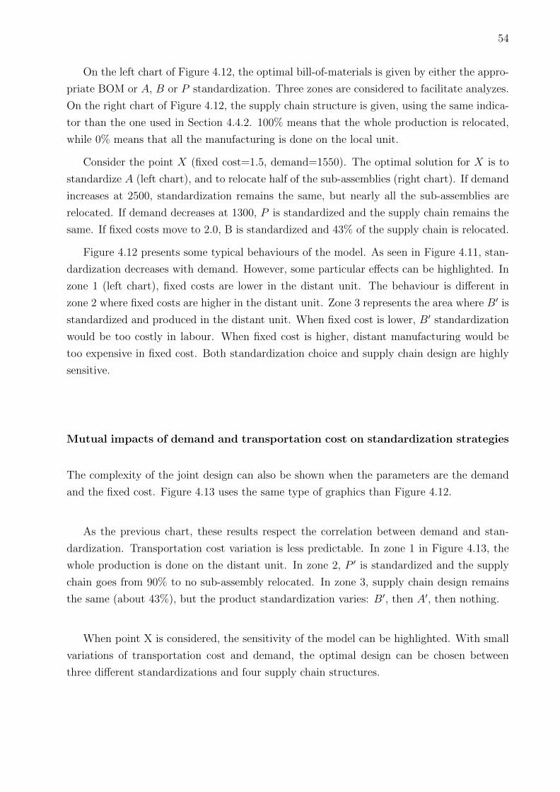
54
On the left chart of Figure 4.12, the optimal bill-of-materials is given by either the appro-
priate BOM or A, B or P standardization. Three zones are considered to facilitate analyzes.
On the right chart of Figure 4.12, the supply chain structure is given, using the same indica-
tor than the one used in Section 4.4.2. 100% means that the whole production is relocated,
while 0% means that all the manufacturing is done on the local unit.
Consider the point X (fixed cost=1.5, demand=1550). The optimal solution for X is to
standardize A (left chart), and to relocate half of the sub-assemblies (right chart). If demand
increases at 2500, standardization remains the same, but nearly all the sub-assemblies are
relocated. If demand decreases at 1300, P is standardized and the supply chain remains the
same. If fixed costs move to 2.0, B is standardized and 43% of the supply chain is relocated.
Figure 4.12 presents some typical behaviours of the model. As seen in Figure 4.11, stan-
dardization decreases with demand. However, some particular effects can be highlighted. In
zone 1 (left chart), fixed costs are lower in the distant unit. The behaviour is different in
zone 2 where fixed costs are higher in the distant unit. Zone 3 represents the area where B′ is
standardized and produced in the distant unit. When fixed cost is lower, B′ standardization
would be too costly in labour. When fixed cost is higher, distant manufacturing would be
too expensive in fixed cost. Both standardization choice and supply chain design are highly
sensitive.
Mutual impacts of demand and transportation cost on standardization strategies
The complexity of the joint design can also be shown when the parameters are the demand
and the fixed cost. Figure 4.13 uses the same type of graphics than Figure 4.12.
As the previous chart, these results respect the correlation between demand and stan-
dardization. Transportation cost variation is less predictable. In zone 1 in Figure 4.13, the
whole production is done on the distant unit. In zone 2, P ′ is standardized and the supply
chain goes from 90% to no sub-assembly relocated. In zone 3, supply chain design remains
the same (about 43%), but the product standardization varies: B′, then A′, then nothing.
When point X is considered, the sensitivity of the model can be highlighted. With small
variations of transportation cost and demand, the optimal design can be chosen between
three different standardizations and four supply chain structures.
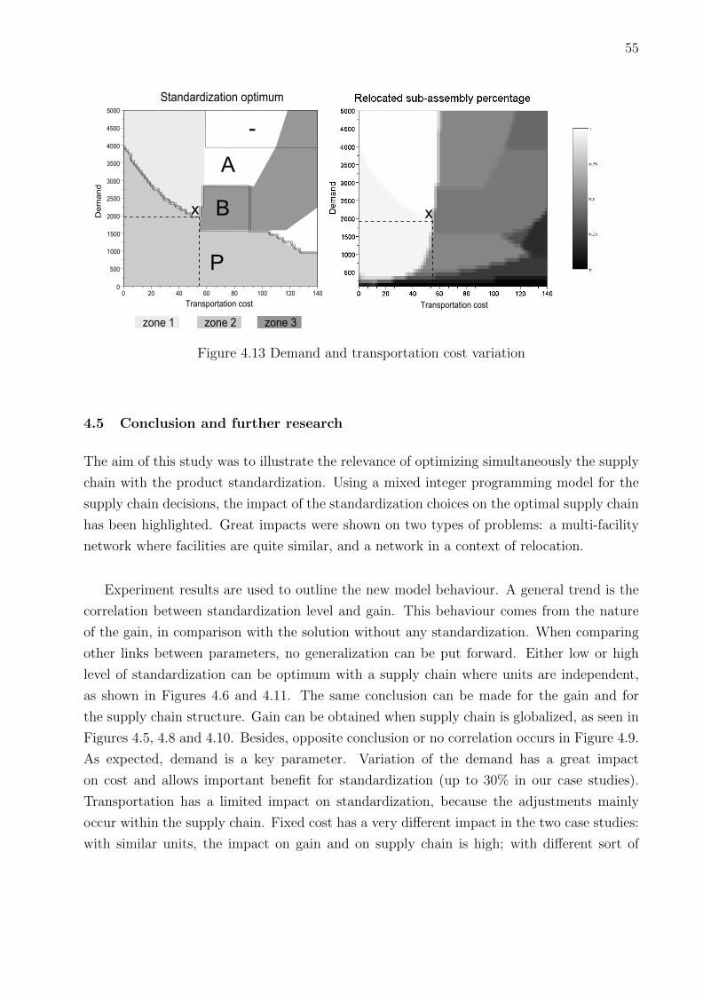
55
x
Transportation cost
0 20 40 80 14060 120
De
man
d
5000
4500
4000
3500
3000
2500
2000
1500
1000
500
0100
Standardization optimum
zone 1 zone 2 zone 3
x
P
B
-
A
Transportation cost
Figure 4.13 Demand and transportation cost variation
4.5 Conclusion and further research
The aim of this study was to illustrate the relevance of optimizing simultaneously the supply
chain with the product standardization. Using a mixed integer programming model for the
supply chain decisions, the impact of the standardization choices on the optimal supply chain
has been highlighted. Great impacts were shown on two types of problems: a multi-facility
network where facilities are quite similar, and a network in a context of relocation.
Experiment results are used to outline the new model behaviour. A general trend is the
correlation between standardization level and gain. This behaviour comes from the nature
of the gain, in comparison with the solution without any standardization. When comparing
other links between parameters, no generalization can be put forward. Either low or high
level of standardization can be optimum with a supply chain where units are independent,
as shown in Figures 4.6 and 4.11. The same conclusion can be made for the gain and for
the supply chain structure. Gain can be obtained when supply chain is globalized, as seen in
Figures 4.5, 4.8 and 4.10. Besides, opposite conclusion or no correlation occurs in Figure 4.9.
As expected, demand is a key parameter. Variation of the demand has a great impact
on cost and allows important benefit for standardization (up to 30% in our case studies).
Transportation has a limited impact on standardization, because the adjustments mainly
occur within the supply chain. Fixed cost has a very different impact in the two case studies:
with similar units, the impact on gain and on supply chain is high; with different sort of
56
units, fixed cost plays yet a role on the supply chain structure, but the impact on the gain is
very limited.
A small example shoved that simultaneous decisions on standardization and on the sup-
ply chain structure may lead to better situations than sequential optimizations. This has
been highlighted by different experiments. The impact of standardization can be huge in
terms of cost. The issue is that the decision changes quickly when some parameters of the
problem vary. Although the trends may sometime be anticipated, some behaviours can be
difficult to predict. The complexity of the global optimization is shown with the 3D-charts
of Figures 4.12 and 4.13.
There is a strong challenge to work on this problem because potential gains can be huge.
When only a few sub-assemblies can be standardized, all possible configurations can be tested
for standardization. For each configuration, the ideal structure of the supply chain and the
cost can be determined. This method has been used for these experimentations. However,
when standardization possibilities are numerous, it becomes necessary to include the stan-
dardization options in the mathematical model. The complexity of the model implies a
thorough search for effective methods in order to improve routing.
As the decisions are very sensitive to variations of the parameters, it would be inter-
esting to develop tools which allow sensitivity analysis of the proposed solutions. Fig-
ures 4.12 and 4.13 show that certain points are at the frontiers of three or four zones, each
zone corresponding to a different strategy in terms of standardization and allocation of pro-
duction. The aim would thus be to determine, for each parameter, an interval within which
the overall decision remains stable.
The more challenging perspective of this work is to model the combined problem consid-
ering simultaneously the product standardization and the product allocation. This problem
can be expressed as a MILP. However, the solution is highly complex due to the increase in
the number of variables and constraints, each standardization possibility producing a new
binary decision variable. Particular interests have to be given on solution methods. An iter-
ative method which optimizes sequentially product and supply chain could be investigated,
but with the risk to never find an optimal solution.
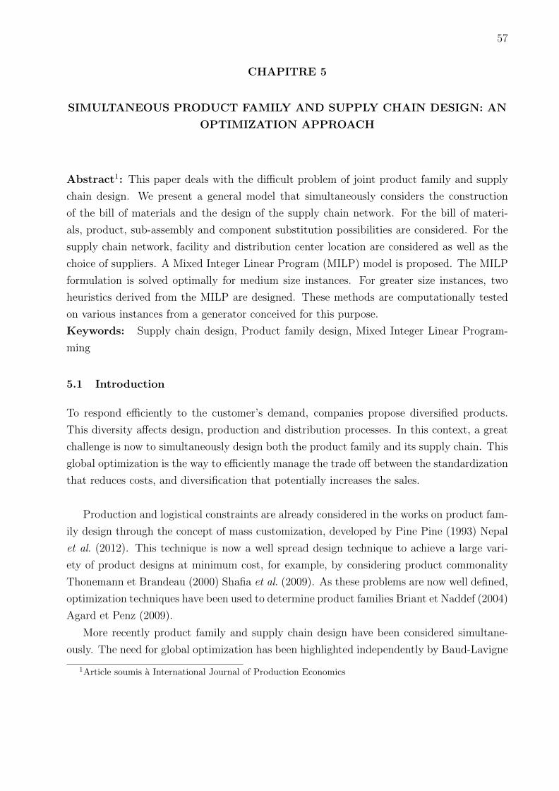
57
CHAPITRE 5
SIMULTANEOUS PRODUCT FAMILY AND SUPPLY CHAIN DESIGN: AN
OPTIMIZATION APPROACH
Abstract1: This paper deals with the difficult problem of joint product family and supply
chain design. We present a general model that simultaneously considers the construction
of the bill of materials and the design of the supply chain network. For the bill of materi-
als, product, sub-assembly and component substitution possibilities are considered. For the
supply chain network, facility and distribution center location are considered as well as the
choice of suppliers. A Mixed Integer Linear Program (MILP) model is proposed. The MILP
formulation is solved optimally for medium size instances. For greater size instances, two
heuristics derived from the MILP are designed. These methods are computationally tested
on various instances from a generator conceived for this purpose.
Keywords: Supply chain design, Product family design, Mixed Integer Linear Program-
ming
5.1 Introduction
To respond efficiently to the customer’s demand, companies propose diversified products.
This diversity affects design, production and distribution processes. In this context, a great
challenge is now to simultaneously design both the product family and its supply chain. This
global optimization is the way to efficiently manage the trade off between the standardization
that reduces costs, and diversification that potentially increases the sales.
Production and logistical constraints are already considered in the works on product fam-
ily design through the concept of mass customization, developed by Pine Pine (1993) Nepal
et al. (2012). This technique is now a well spread design technique to achieve a large vari-
ety of product designs at minimum cost, for example, by considering product commonality
Thonemann et Brandeau (2000) Shafia et al. (2009). As these problems are now well defined,
optimization techniques have been used to determine product families Briant et Naddef (2004)
Agard et Penz (2009).
More recently product family and supply chain design have been considered simultane-
ously. The need for global optimization has been highlighted independently by Baud-Lavigne
1Article soumis a International Journal of Production Economics
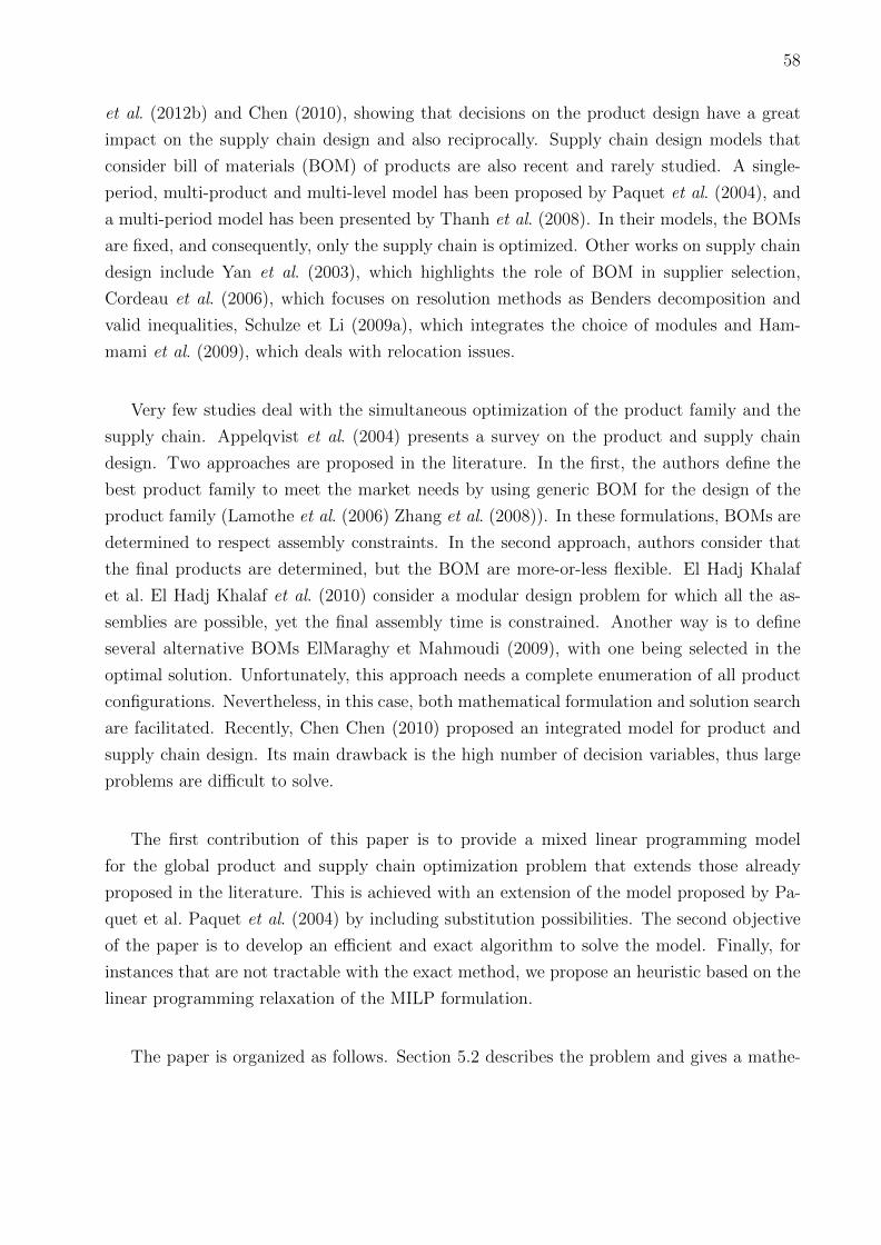
58
et al. (2012b) and Chen (2010), showing that decisions on the product design have a great
impact on the supply chain design and also reciprocally. Supply chain design models that
consider bill of materials (BOM) of products are also recent and rarely studied. A single-
period, multi-product and multi-level model has been proposed by Paquet et al. (2004), and
a multi-period model has been presented by Thanh et al. (2008). In their models, the BOMs
are fixed, and consequently, only the supply chain is optimized. Other works on supply chain
design include Yan et al. (2003), which highlights the role of BOM in supplier selection,
Cordeau et al. (2006), which focuses on resolution methods as Benders decomposition and
valid inequalities, Schulze et Li (2009a), which integrates the choice of modules and Ham-
mami et al. (2009), which deals with relocation issues.
Very few studies deal with the simultaneous optimization of the product family and the
supply chain. Appelqvist et al. (2004) presents a survey on the product and supply chain
design. Two approaches are proposed in the literature. In the first, the authors define the
best product family to meet the market needs by using generic BOM for the design of the
product family (Lamothe et al. (2006) Zhang et al. (2008)). In these formulations, BOMs are
determined to respect assembly constraints. In the second approach, authors consider that
the final products are determined, but the BOM are more-or-less flexible. El Hadj Khalaf
et al. El Hadj Khalaf et al. (2010) consider a modular design problem for which all the as-
semblies are possible, yet the final assembly time is constrained. Another way is to define
several alternative BOMs ElMaraghy et Mahmoudi (2009), with one being selected in the
optimal solution. Unfortunately, this approach needs a complete enumeration of all product
configurations. Nevertheless, in this case, both mathematical formulation and solution search
are facilitated. Recently, Chen Chen (2010) proposed an integrated model for product and
supply chain design. Its main drawback is the high number of decision variables, thus large
problems are difficult to solve.
The first contribution of this paper is to provide a mixed linear programming model
for the global product and supply chain optimization problem that extends those already
proposed in the literature. This is achieved with an extension of the model proposed by Pa-
quet et al. Paquet et al. (2004) by including substitution possibilities. The second objective
of the paper is to develop an efficient and exact algorithm to solve the model. Finally, for
instances that are not tractable with the exact method, we propose an heuristic based on the
linear programming relaxation of the MILP formulation.
The paper is organized as follows. Section 5.2 describes the problem and gives a mathe-
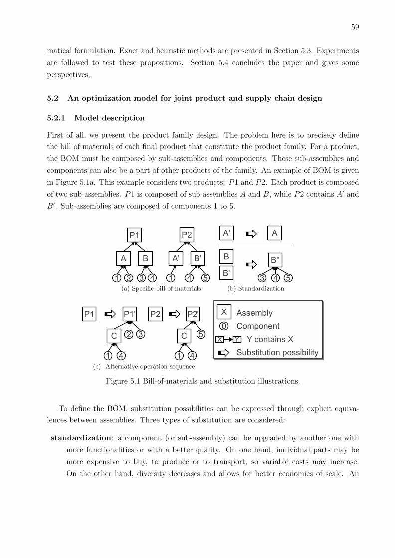
59
matical formulation. Exact and heuristic methods are presented in Section 5.3. Experiments
are followed to test these propositions. Section 5.4 concludes the paper and gives some
perspectives.
5.2 An optimization model for joint product and supply chain design
5.2.1 Model description
First of all, we present the product family design. The problem here is to precisely define
the bill of materials of each final product that constitute the product family. For a product,
the BOM must be composed by sub-assemblies and components. These sub-assemblies and
components can also be a part of other products of the family. An example of BOM is given
in Figure 5.1a. This example considers two products: P1 and P2. Each product is composed
of two sub-assemblies. P1 is composed of sub-assemblies A and B, while P2 contains A′ and
B′. Sub-assemblies are composed of components 1 to 5.
(a) Specific bill-of-materials (b) Standardization
(c) Alternative operation sequence
Figure 5.1 Bill-of-materials and substitution illustrations.
To define the BOM, substitution possibilities can be expressed through explicit equiva-
lences between assemblies. Three types of substitution are considered:
standardization: a component (or sub-assembly) can be upgraded by another one with
more functionalities or with a better quality. On one hand, individual parts may be
more expensive to buy, to produce or to transport, so variable costs may increase.
On the other hand, diversity decreases and allows for better economies of scale. An
60
illustration is provided in Figure 5.1b. Sub-assembly A′ can be replaced by A, B and
B′ can be replaced by a new sub-assembly B′′,
externalization: a sub-assembly is bought directly from a subcontractor. While avoiding
production line, fixed costs are minimized and variable costs may increase because the
subcontractor has to invest. Thus each unit should be sold at a higher price than if it
was made internally. In the example in Figure 5.1a, the sub-assembly A or B can be
replaced by a component bought from a supplier,
alternative operating sequence/product decomposition: other component assem-
bling sequences can permit better commonality without necessarily changing costs.
Figure 5.1c presents a sequence where sub-assembly C has a better commonality with-
out adding extra function.
These possible substitutions of sub-assemblies or components in the BOM introduce a
difficulty in the modeling. A typical way to express substitution is to use the BOM as a
decision variable. This way leads to quadratic constraints between BOM and production de-
cision variables in most supply chain design models. Another way, proposed in Chen (2010),
is to use decision variables to express exactly which quantity of each alternative is used for
each assembly produced. This leads to a considerable amount of decision variables. In our
model, we simplify the approach. The product substitution is considered through product
transformation. When part X is able to substitute part Y , a virtual process can transform
X into Y . Then, a quantity of X on a plant is mixed between actual X parts and alterna-
tives that have been transformed into Y . This modeling allows substitution while keeping
a light formulation. Indeed, the number of additional variables is exactly the substitution
possibilities.
Concerning the supply chain design, we consider a generic supply chain as depicted in
Figure 5.2. In the generic supply chain, there are four layers: suppliers, production centers,
distribution centers and customers. This example shows a supply chain with four suppliers,
three production centers, three distribution centers and four customers. Flows contain only
components between the suppliers and the production centers. They also only contain prod-
ucts between the plants and the customers and all types of parts (components, assemblies
and products) between the different production centers. Workstations are also allocated to
each production center.
The manufacture of each sub-assembly or product may require some specific technologies.
For each technology, different options may be available. For example, for an assembly, we can
propose a totally manual workstation (option 1) with a certain capacity, or a fully automated
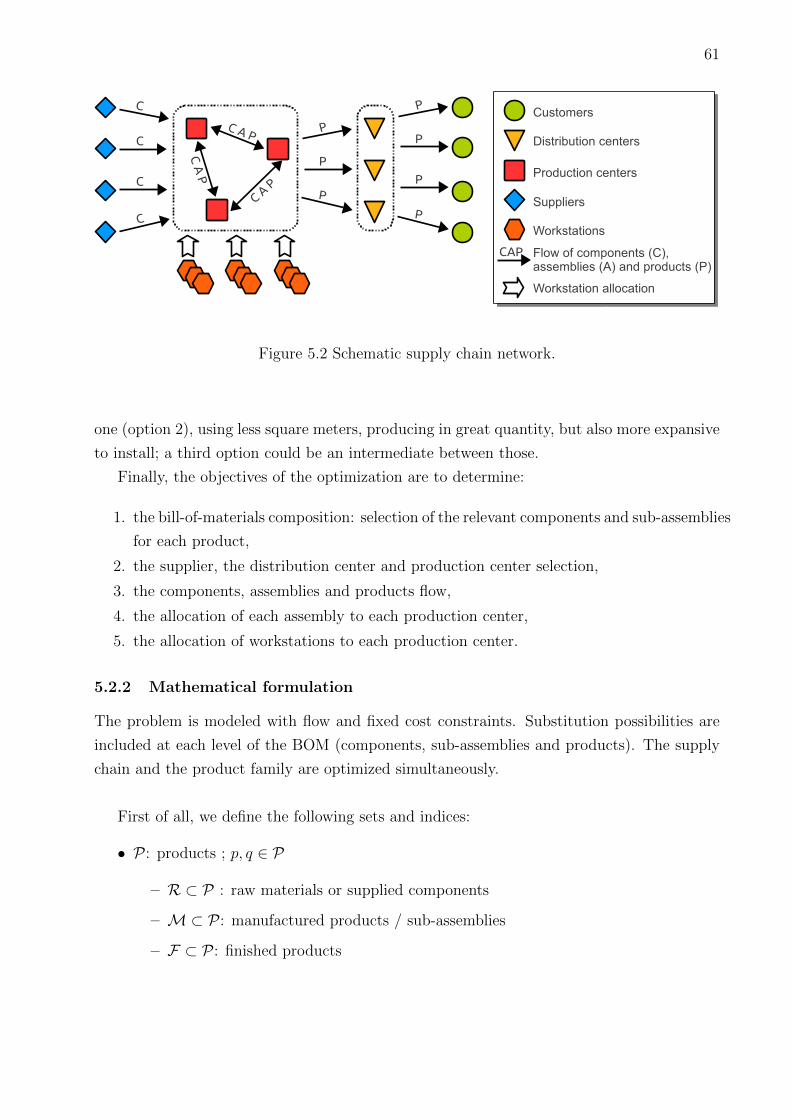
61
Figure 5.2 Schematic supply chain network.
one (option 2), using less square meters, producing in great quantity, but also more expansive
to install; a third option could be an intermediate between those.
Finally, the objectives of the optimization are to determine:
1. the bill-of-materials composition: selection of the relevant components and sub-assemblies
for each product,
2. the supplier, the distribution center and production center selection,
3. the components, assemblies and products flow,
4. the allocation of each assembly to each production center,
5. the allocation of workstations to each production center.
5.2.2 Mathematical formulation
The problem is modeled with flow and fixed cost constraints. Substitution possibilities are
included at each level of the BOM (components, sub-assemblies and products). The supply
chain and the product family are optimized simultaneously.
First of all, we define the following sets and indices:
• P : products ; p, q ∈ P
– R ⊂ P : raw materials or supplied components
– M⊂ P : manufactured products / sub-assemblies
– F ⊂ P : finished products
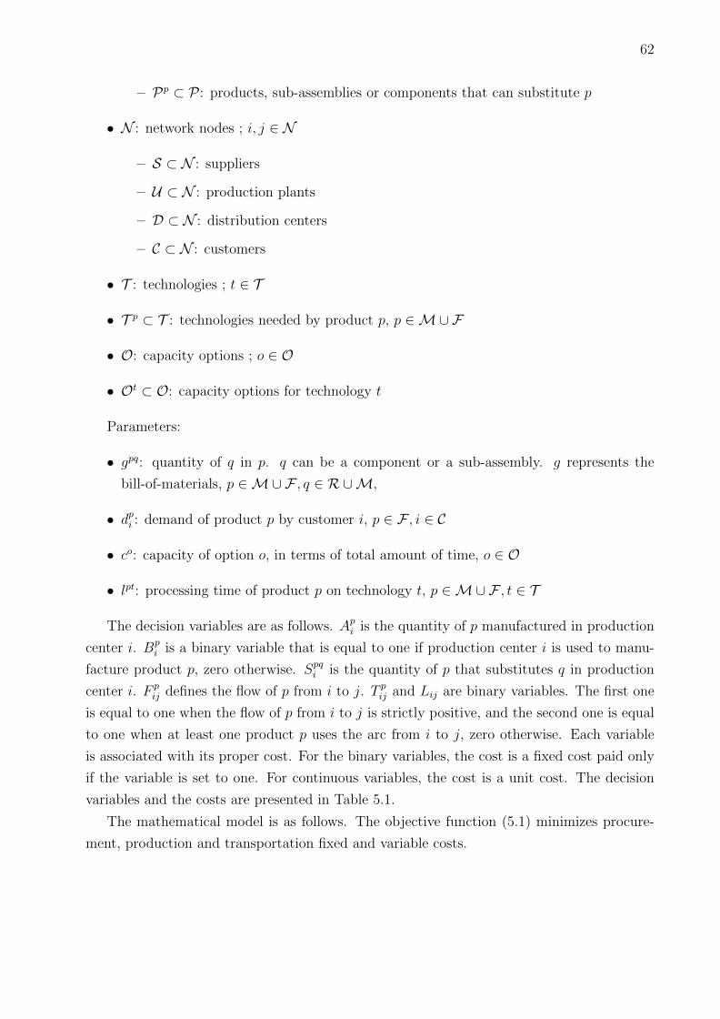
62
– Pp ⊂ P : products, sub-assemblies or components that can substitute p
• N : network nodes ; i, j ∈ N
– S ⊂ N : suppliers
– U ⊂ N : production plants
– D ⊂ N : distribution centers
– C ⊂ N : customers
• T : technologies ; t ∈ T
• T p ⊂ T : technologies needed by product p, p ∈M∪F
• O: capacity options ; o ∈ O
• Ot ⊂ O: capacity options for technology t
Parameters:
• gpq: quantity of q in p. q can be a component or a sub-assembly. g represents the
bill-of-materials, p ∈M∪F , q ∈ R ∪M,
• dpi : demand of product p by customer i, p ∈ F , i ∈ C
• co: capacity of option o, in terms of total amount of time, o ∈ O
• lpt: processing time of product p on technology t, p ∈M∪F , t ∈ T
The decision variables are as follows. Api is the quantity of p manufactured in production
center i. Bpi is a binary variable that is equal to one if production center i is used to manu-
facture product p, zero otherwise. Spqi is the quantity of p that substitutes q in production
center i. F pij defines the flow of p from i to j. T p
ij and Lij are binary variables. The first one
is equal to one when the flow of p from i to j is strictly positive, and the second one is equal
to one when at least one product p uses the arc from i to j, zero otherwise. Each variable
is associated with its proper cost. For the binary variables, the cost is a fixed cost paid only
if the variable is set to one. For continuous variables, the cost is a unit cost. The decision
variables and the costs are presented in Table 5.1.
The mathematical model is as follows. The objective function (5.1) minimizes procure-
ment, production and transportation fixed and variable costs.
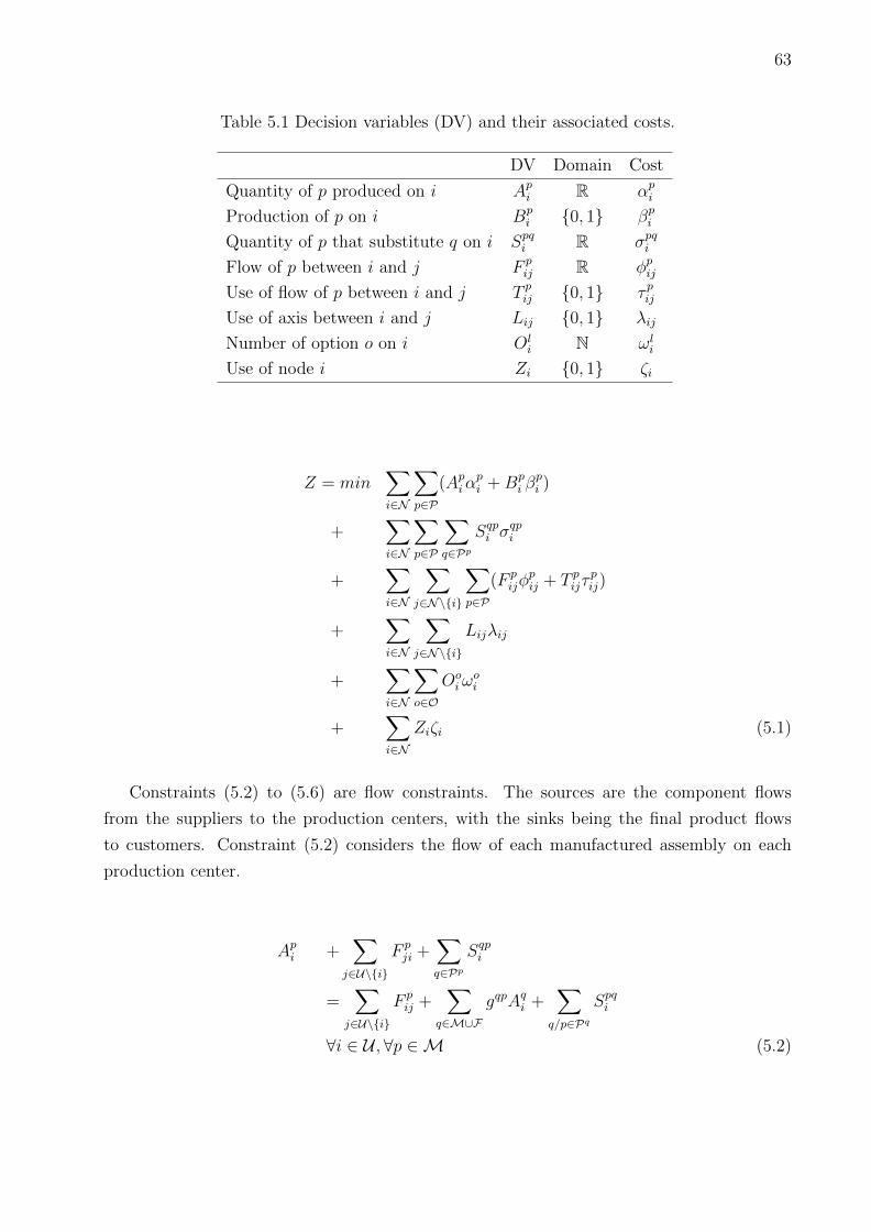
63
Table 5.1 Decision variables (DV) and their associated costs.
DV Domain Cost
Quantity of p produced on i Api R αp
i
Production of p on i Bpi {0, 1} βp
i
Quantity of p that substitute q on i Spqi R σpq
i
Flow of p between i and j F pij R φp
ij
Use of flow of p between i and j T pij {0, 1} τ pij
Use of axis between i and j Lij {0, 1} λij
Number of option o on i Oli N ωl
i
Use of node i Zi {0, 1} ζi
Z = min∑i∈N
∑p∈P
(Apiα
pi +Bp
i βpi )
+∑i∈N
∑p∈P
∑q∈Pp
Sqpi σ
qpi
+∑i∈N
∑j∈N\{i}
∑p∈P
(F pijφ
pij + T p
ijτpij)
+∑i∈N
∑j∈N\{i}
Lijλij
+∑i∈N
∑o∈O
Ooiω
oi
+∑i∈N
Ziζi (5.1)
Constraints (5.2) to (5.6) are flow constraints. The sources are the component flows
from the suppliers to the production centers, with the sinks being the final product flows
to customers. Constraint (5.2) considers the flow of each manufactured assembly on each
production center.
Api +
∑j∈U\{i}
F pji +
∑q∈Pp
Sqpi
=∑
j∈U\{i}
F pij +
∑q∈M∪F
gqpAqi +
∑q/p∈Pq
Spqi
∀i ∈ U ,∀p ∈M (5.2)
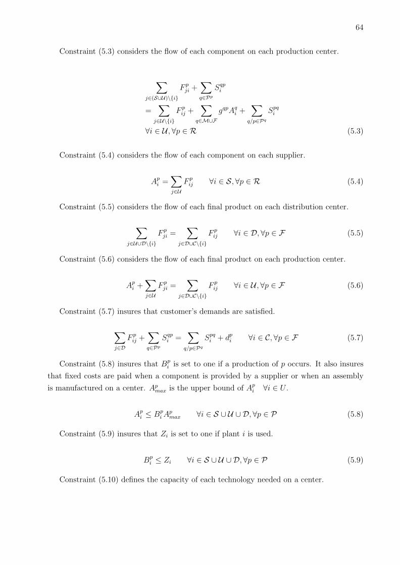
64
Constraint (5.3) considers the flow of each component on each production center.
∑j∈(S∪U)\{i}
F pji +
∑q∈Pp
Sqpi
=∑
j∈U\{i}
F pij +
∑q∈M∪F
gqpAqi +
∑q/p∈Pq
Spqi
∀i ∈ U ,∀p ∈ R (5.3)
Constraint (5.4) considers the flow of each component on each supplier.
Api =
∑j∈U
F pij ∀i ∈ S,∀p ∈ R (5.4)
Constraint (5.5) considers the flow of each final product on each distribution center.
∑j∈U∪D\{i}
F pji =
∑j∈D∪C\{i}
F pij ∀i ∈ D,∀p ∈ F (5.5)
Constraint (5.6) considers the flow of each final product on each production center.
Api +
∑j∈U
F pji =
∑j∈D∪C\{i}
F pij ∀i ∈ U ,∀p ∈ F (5.6)
Constraint (5.7) insures that customer’s demands are satisfied.
∑j∈D
F pij +
∑q∈Pp
Sqpi =
∑q/p∈Pq
Spqi + dpi ∀i ∈ C,∀p ∈ F (5.7)
Constraint (5.8) insures that Bpi is set to one if a production of p occurs. It also insures
that fixed costs are paid when a component is provided by a supplier or when an assembly
is manufactured on a center. Apmax is the upper bound of Ap
i ∀i ∈ U .
Api ≤ Bp
iApmax ∀i ∈ S ∪ U ∪ D, ∀p ∈ P (5.8)
Constraint (5.9) insures that Zi is set to one if plant i is used.
Bpi ≤ Zi ∀i ∈ S ∪ U ∪ D,∀p ∈ P (5.9)
Constraint (5.10) defines the capacity of each technology needed on a center.
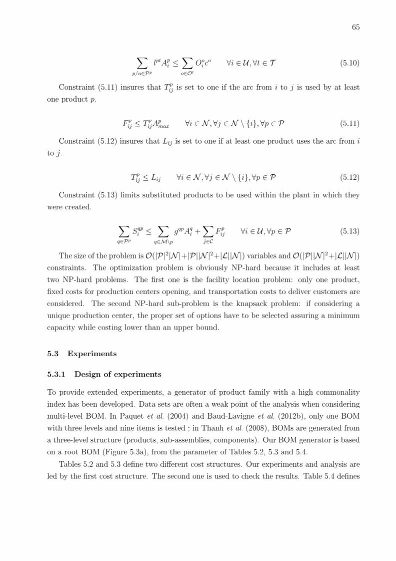
65
∑p/u∈Pp
lptApi ≤
∑o∈Ot
Ooi c
o ∀i ∈ U , ∀t ∈ T (5.10)
Constraint (5.11) insures that T pij is set to one if the arc from i to j is used by at least
one product p.
F pij ≤ T p
ijApmax ∀i ∈ N ,∀j ∈ N \ {i}, ∀p ∈ P (5.11)
Constraint (5.12) insures that Lij is set to one if at least one product uses the arc from i
to j.
T pij ≤ Lij ∀i ∈ N ,∀j ∈ N \ {i}, ∀p ∈ P (5.12)
Constraint (5.13) limits substituted products to be used within the plant in which they
were created.
∑q∈Pp
Sqpi ≤
∑q∈M\p
gqpAqi +
∑j∈C
F pij ∀i ∈ U ,∀p ∈ P (5.13)
The size of the problem isO(|P|2|N |+|P||N |2+|L||N |) variables andO(|P||N |2+|L||N |)constraints. The optimization problem is obviously NP-hard because it includes at least
two NP-hard problems. The first one is the facility location problem: only one product,
fixed costs for production centers opening, and transportation costs to deliver customers are
considered. The second NP-hard sub-problem is the knapsack problem: if considering a
unique production center, the proper set of options have to be selected assuring a minimum
capacity while costing lower than an upper bound.
5.3 Experiments
5.3.1 Design of experiments
To provide extended experiments, a generator of product family with a high commonality
index has been developed. Data sets are often a weak point of the analysis when considering
multi-level BOM. In Paquet et al. (2004) and Baud-Lavigne et al. (2012b), only one BOM
with three levels and nine items is tested ; in Thanh et al. (2008), BOMs are generated from
a three-level structure (products, sub-assemblies, components). Our BOM generator is based
on a root BOM (Figure 5.3a), from the parameter of Tables 5.2, 5.3 and 5.4.
Tables 5.2 and 5.3 define two different cost structures. Our experiments and analysis are
led by the first cost structure. The second one is used to check the results. Table 5.4 defines
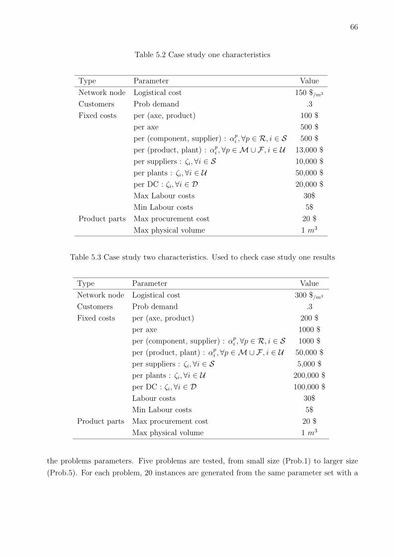
66
Table 5.2 Case study one characteristics
Type Parameter Value
Network node Logistical cost 150 $/m3
Customers Prob demand .3
Fixed costs per (axe, product) 100 $
per axe 500 $
per (component, supplier) : αpi ,∀p ∈ R, i ∈ S 500 $
per (product, plant) : αpi ,∀p ∈M∪F , i ∈ U 13,000 $
per suppliers : ζi,∀i ∈ S 10,000 $
per plants : ζi,∀i ∈ U 50,000 $
per DC : ζi,∀i ∈ D 20,000 $
Max Labour costs 30$
Min Labour costs 5$
Product parts Max procurement cost 20 $
Max physical volume 1 m3
Table 5.3 Case study two characteristics. Used to check case study one results
Type Parameter Value
Network node Logistical cost 300 $/m3
Customers Prob demand .3
Fixed costs per (axe, product) 200 $
per axe 1000 $
per (component, supplier) : αpi ,∀p ∈ R, i ∈ S 1000 $
per (product, plant) : αpi ,∀p ∈M∪F , i ∈ U 50,000 $
per suppliers : ζi,∀i ∈ S 5,000 $
per plants : ζi,∀i ∈ U 200,000 $
per DC : ζi, ∀i ∈ D 100,000 $
Labour costs 30$
Min Labour costs 5$
Product parts Max procurement cost 20 $
Max physical volume 1 m3
the problems parameters. Five problems are tested, from small size (Prob.1) to larger size
(Prob.5). For each problem, 20 instances are generated from the same parameter set with a
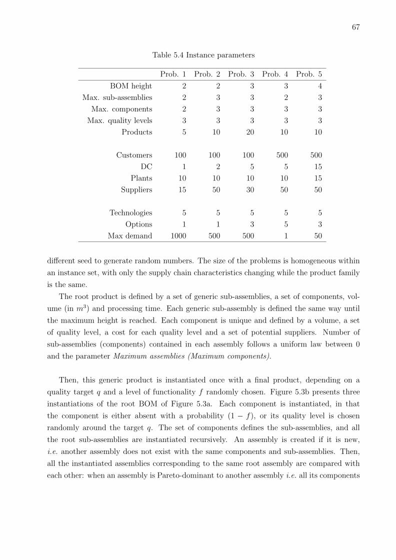
67
Table 5.4 Instance parameters
Prob. 1 Prob. 2 Prob. 3 Prob. 4 Prob. 5
BOM height 2 2 3 3 4
Max. sub-assemblies 2 3 3 2 3
Max. components 2 3 3 3 3
Max. quality levels 3 3 3 3 3
Products 5 10 20 10 10
Customers 100 100 100 500 500
DC 1 2 5 5 15
Plants 10 10 10 10 15
Suppliers 15 50 30 50 50
Technologies 5 5 5 5 5
Options 1 1 3 5 3
Max demand 1000 500 500 1 50
different seed to generate random numbers. The size of the problems is homogeneous within
an instance set, with only the supply chain characteristics changing while the product family
is the same.
The root product is defined by a set of generic sub-assemblies, a set of components, vol-
ume (in m3) and processing time. Each generic sub-assembly is defined the same way until
the maximum height is reached. Each component is unique and defined by a volume, a set
of quality level, a cost for each quality level and a set of potential suppliers. Number of
sub-assemblies (components) contained in each assembly follows a uniform law between 0
and the parameter Maximum assemblies (Maximum components).
Then, this generic product is instantiated once with a final product, depending on a
quality target q and a level of functionality f randomly chosen. Figure 5.3b presents three
instantiations of the root BOM of Figure 5.3a. Each component is instantiated, in that
the component is either absent with a probability (1 − f), or its quality level is chosen
randomly around the target q. The set of components defines the sub-assemblies, and all
the root sub-assemblies are instantiated recursively. An assembly is created if it is new,
i.e. another assembly does not exist with the same components and sub-assemblies. Then,
all the instantiated assemblies corresponding to the same root assembly are compared with
each other: when an assembly is Pareto-dominant to another assembly i.e. all its components
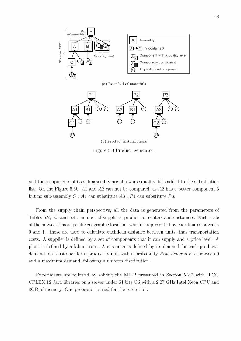
68
(a) Root bill-of-materials
(b) Product instantiations
Figure 5.3 Product generator.
and the components of its sub-assembly are of a worse quality, it is added to the substitution
list. On the Figure 5.3b, A1 and A2 can not be compared, as A2 has a better component 3
but no sub-assembly C ; A1 can substitute A3 ; P1 can substitute P3.
From the supply chain perspective, all the data is generated from the parameters of
Tables 5.2, 5.3 and 5.4 : number of suppliers, production centers and customers. Each node
of the network has a specific geographic location, which is represented by coordinates between
0 and 1 ; those are used to calculate euclidean distance between units, thus transportation
costs. A supplier is defined by a set of components that it can supply and a price level. A
plant is defined by a labour rate. A customer is defined by its demand for each product :
demand of a customer for a product is null with a probability Prob demand else between 0
and a maximum demand, following a uniform distribution.
Experiments are followed by solving the MILP presented in Section 5.2.2 with ILOG
CPLEX 12 Java libraries on a server under 64 bits OS with a 2.27 GHz Intel Xeon CPU and
8GB of memory. One processor is used for the resolution.
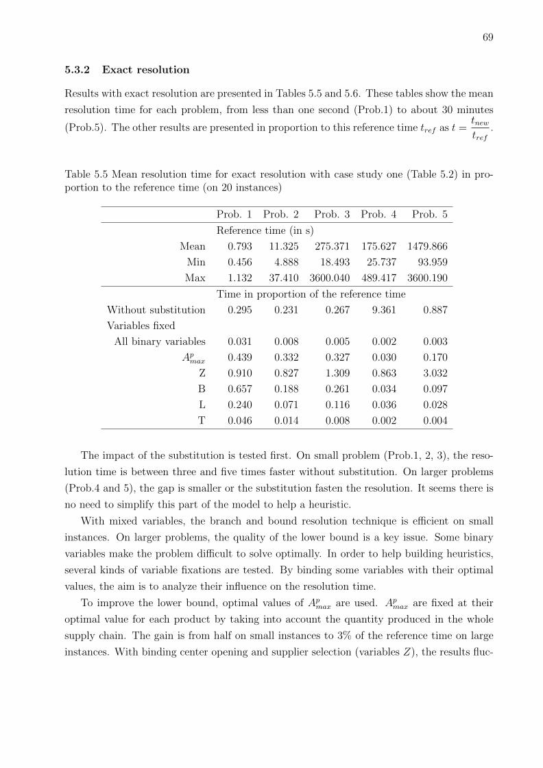
69
5.3.2 Exact resolution
Results with exact resolution are presented in Tables 5.5 and 5.6. These tables show the mean
resolution time for each problem, from less than one second (Prob.1) to about 30 minutes
(Prob.5). The other results are presented in proportion to this reference time tref as t =tnewtref
.
Table 5.5 Mean resolution time for exact resolution with case study one (Table 5.2) in pro-portion to the reference time (on 20 instances)
Prob. 1 Prob. 2 Prob. 3 Prob. 4 Prob. 5
Reference time (in s)
Mean 0.793 11.325 275.371 175.627 1479.866
Min 0.456 4.888 18.493 25.737 93.959
Max 1.132 37.410 3600.040 489.417 3600.190
Time in proportion of the reference time
Without substitution 0.295 0.231 0.267 9.361 0.887
Variables fixed
All binary variables 0.031 0.008 0.005 0.002 0.003
Apmax 0.439 0.332 0.327 0.030 0.170
Z 0.910 0.827 1.309 0.863 3.032
B 0.657 0.188 0.261 0.034 0.097
L 0.240 0.071 0.116 0.036 0.028
T 0.046 0.014 0.008 0.002 0.004
The impact of the substitution is tested first. On small problem (Prob.1, 2, 3), the reso-
lution time is between three and five times faster without substitution. On larger problems
(Prob.4 and 5), the gap is smaller or the substitution fasten the resolution. It seems there is
no need to simplify this part of the model to help a heuristic.
With mixed variables, the branch and bound resolution technique is efficient on small
instances. On larger problems, the quality of the lower bound is a key issue. Some binary
variables make the problem difficult to solve optimally. In order to help building heuristics,
several kinds of variable fixations are tested. By binding some variables with their optimal
values, the aim is to analyze their influence on the resolution time.
To improve the lower bound, optimal values of Apmax are used. Ap
max are fixed at their
optimal value for each product by taking into account the quantity produced in the whole
supply chain. The gain is from half on small instances to 3% of the reference time on large
instances. With binding center opening and supplier selection (variables Z), the results fluc-
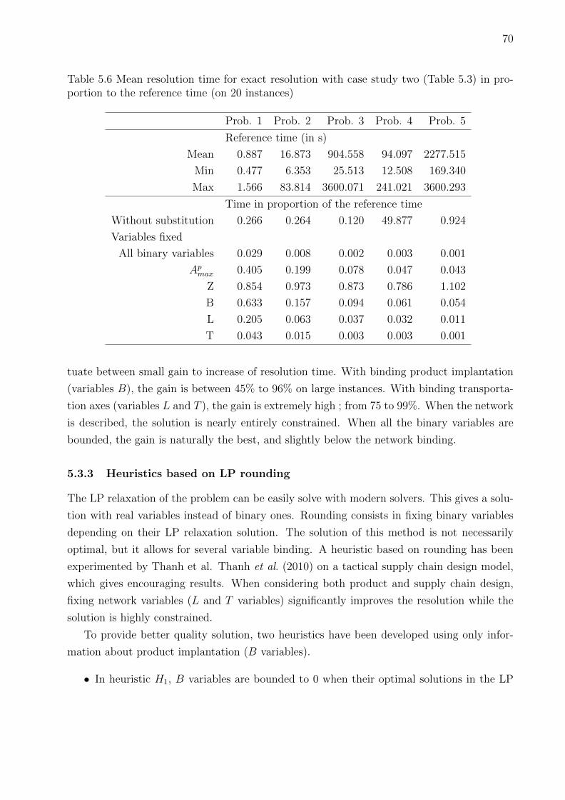
70
Table 5.6 Mean resolution time for exact resolution with case study two (Table 5.3) in pro-portion to the reference time (on 20 instances)
Prob. 1 Prob. 2 Prob. 3 Prob. 4 Prob. 5
Reference time (in s)
Mean 0.887 16.873 904.558 94.097 2277.515
Min 0.477 6.353 25.513 12.508 169.340
Max 1.566 83.814 3600.071 241.021 3600.293
Time in proportion of the reference time
Without substitution 0.266 0.264 0.120 49.877 0.924
Variables fixed
All binary variables 0.029 0.008 0.002 0.003 0.001
Apmax 0.405 0.199 0.078 0.047 0.043
Z 0.854 0.973 0.873 0.786 1.102
B 0.633 0.157 0.094 0.061 0.054
L 0.205 0.063 0.037 0.032 0.011
T 0.043 0.015 0.003 0.003 0.001
tuate between small gain to increase of resolution time. With binding product implantation
(variables B), the gain is between 45% to 96% on large instances. With binding transporta-
tion axes (variables L and T ), the gain is extremely high ; from 75 to 99%. When the network
is described, the solution is nearly entirely constrained. When all the binary variables are
bounded, the gain is naturally the best, and slightly below the network binding.
5.3.3 Heuristics based on LP rounding
The LP relaxation of the problem can be easily solve with modern solvers. This gives a solu-
tion with real variables instead of binary ones. Rounding consists in fixing binary variables
depending on their LP relaxation solution. The solution of this method is not necessarily
optimal, but it allows for several variable binding. A heuristic based on rounding has been
experimented by Thanh et al. Thanh et al. (2010) on a tactical supply chain design model,
which gives encouraging results. When considering both product and supply chain design,
fixing network variables (L and T variables) significantly improves the resolution while the
solution is highly constrained.
To provide better quality solution, two heuristics have been developed using only infor-
mation about product implantation (B variables).
• In heuristic H1, B variables are bounded to 0 when their optimal solutions in the LP
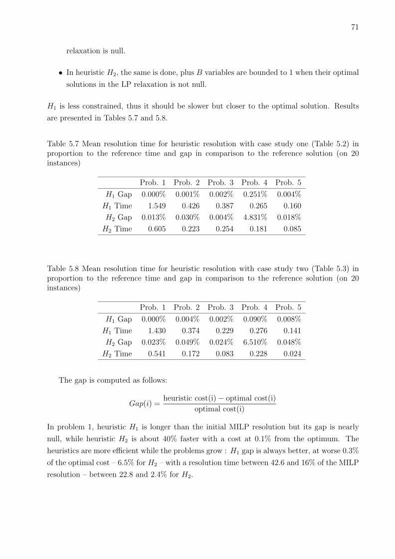
71
relaxation is null.
• In heuristic H2, the same is done, plus B variables are bounded to 1 when their optimal
solutions in the LP relaxation is not null.
H1 is less constrained, thus it should be slower but closer to the optimal solution. Results
are presented in Tables 5.7 and 5.8.
Table 5.7 Mean resolution time for heuristic resolution with case study one (Table 5.2) inproportion to the reference time and gap in comparison to the reference solution (on 20instances)
Prob. 1 Prob. 2 Prob. 3 Prob. 4 Prob. 5
H1 Gap 0.000% 0.001% 0.002% 0.251% 0.004%
H1 Time 1.549 0.426 0.387 0.265 0.160
H2 Gap 0.013% 0.030% 0.004% 4.831% 0.018%
H2 Time 0.605 0.223 0.254 0.181 0.085
Table 5.8 Mean resolution time for heuristic resolution with case study two (Table 5.3) inproportion to the reference time and gap in comparison to the reference solution (on 20instances)
Prob. 1 Prob. 2 Prob. 3 Prob. 4 Prob. 5
H1 Gap 0.000% 0.004% 0.002% 0.090% 0.008%
H1 Time 1.430 0.374 0.229 0.276 0.141
H2 Gap 0.023% 0.049% 0.024% 6.510% 0.048%
H2 Time 0.541 0.172 0.083 0.228 0.024
The gap is computed as follows:
Gap(i) =heuristic cost(i)− optimal cost(i)
optimal cost(i)
In problem 1, heuristic H1 is longer than the initial MILP resolution but its gap is nearly
null, while heuristic H2 is about 40% faster with a cost at 0.1% from the optimum. The
heuristics are more efficient while the problems grow : H1 gap is always better, at worse 0.3%
of the optimal cost – 6.5% for H2 – with a resolution time between 42.6 and 16% of the MILP
resolution – between 22.8 and 2.4% for H2.
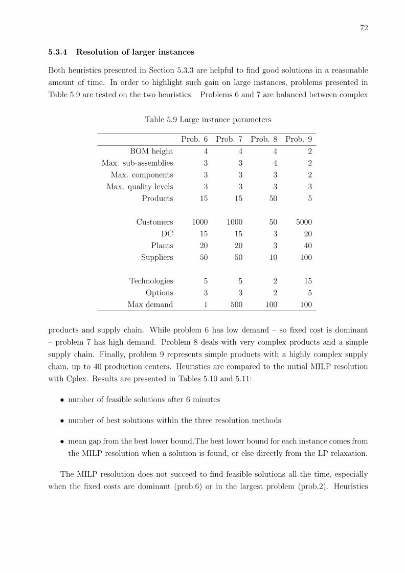
72
5.3.4 Resolution of larger instances
Both heuristics presented in Section 5.3.3 are helpful to find good solutions in a reasonable
amount of time. In order to highlight such gain on large instances, problems presented in
Table 5.9 are tested on the two heuristics. Problems 6 and 7 are balanced between complex
Table 5.9 Large instance parameters
Prob. 6 Prob. 7 Prob. 8 Prob. 9
BOM height 4 4 4 2
Max. sub-assemblies 3 3 4 2
Max. components 3 3 3 2
Max. quality levels 3 3 3 3
Products 15 15 50 5
Customers 1000 1000 50 5000
DC 15 15 3 20
Plants 20 20 3 40
Suppliers 50 50 10 100
Technologies 5 5 2 15
Options 3 3 2 5
Max demand 1 500 100 100
products and supply chain. While problem 6 has low demand – so fixed cost is dominant
– problem 7 has high demand. Problem 8 deals with very complex products and a simple
supply chain. Finally, problem 9 represents simple products with a highly complex supply
chain, up to 40 production centers. Heuristics are compared to the initial MILP resolution
with Cplex. Results are presented in Tables 5.10 and 5.11:
• number of feasible solutions after 6 minutes
• number of best solutions within the three resolution methods
• mean gap from the best lower bound.The best lower bound for each instance comes from
the MILP resolution when a solution is found, or else directly from the LP relaxation.
The MILP resolution does not succeed to find feasible solutions all the time, especially
when the fixed costs are dominant (prob.6) or in the largest problem (prob.2). Heuristics
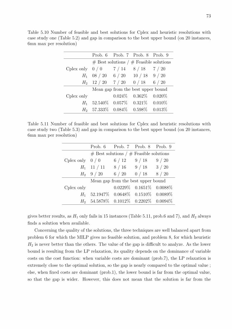
73
Table 5.10 Number of feasible and best solutions for Cplex and heuristic resolutions withcase study one (Table 5.2) and gap in comparison to the best upper bound (on 20 instances,6mn max per resolution)
Prob. 6 Prob. 7 Prob. 8 Prob. 9
# Best solutions / # Feasible solutions
Cplex only 0 / 0 7 / 14 8 / 18 7 / 20
H1 08 / 20 6 / 20 10 / 18 9 / 20
H2 12 / 20 7 / 20 0 / 18 6 / 20
Mean gap from the best upper bound
Cplex only 0.024% 0.362% 0.020%
H1 52.540% 0.057% 0.321% 0.010%
H2 57.333% 0.084% 0.598% 0.013%
Table 5.11 Number of feasible and best solutions for Cplex and heuristic resolutions withcase study two (Table 5.3) and gap in comparison to the best upper bound (on 20 instances,6mn max per resolution)
Prob. 6 Prob. 7 Prob. 8 Prob. 9
# Best solutions / # Feasible solutions
Cplex only 0 / 0 6 / 12 9 / 18 9 / 20
H1 11 / 11 8 / 16 9 / 18 3 / 20
H2 9 / 20 6 / 20 0 / 18 8 / 20
Mean gap from the best upper bound
Cplex only 0.0229% 0.1651% 0.0088%
H1 52.1947% 0.0648% 0.1510% 0.0089%
H2 54.5878% 0.1012% 0.2202% 0.0094%
gives better results, as H1 only fails in 15 instances (Table 5.11, prob.6 and 7), and H2 always
finds a solution when available.
Concerning the quality of the solutions, the three techniques are well balanced apart from
problem 6 for which the MILP gives no feasible solution, and problem 8, for which heuristic
H2 is never better than the others. The value of the gap is difficult to analyze. As the lower
bound is resulting from the LP relaxation, its quality depends on the dominance of variable
costs on the cost function: when variable costs are dominant (prob.7), the LP relaxation is
extremely close to the optimal solution, so the gap is nearly compared to the optimal value ;
else, when fixed costs are dominant (prob.1), the lower bound is far from the optimal value,
so that the gap is wider. However, this does not mean that the solution is far from the
74
optimal solution.
5.4 Conclusion
This paper tackles the difficult problem of joint product family and supply chain design.
This issue has attracted more and more attention in recent years. However, most studies
deal with a specific part of the problem, or they propose intractable models. The aim of this
paper is to integrate product substitution into a supply chain design model without adding
too many variables and constraints. We consider a problem in which the product family
and demand is known and must be satisfied. Decisions include supply chain design – from
the supplier selection, the plant location, the product allocation to their distribution – and
bill-of-materials reconfiguration through substitution possibilities. The breakthrough of this
paper is to consider substitution as product transformation. This allows for a simple inclusion
of the substitution in most supply chain design models and avoids to add much resolution
complexity. Indeed, experiments have shown that substitution does not significantly worsen,
nor improve the resolution. The need for complex BOM generator has been highlighted, and
one methodology is proposed to generate product family BOM as benchmarks. Finally, two
heuristics based on LP rounding have been proposed which gives significant improvement in
resolution length while giving good solutions.
Perspectives include :
• analysis of real case studies to characterize solution behaviours and to develop a decision-
making tool. We need to determine the key variables and study the sensitivity of the
solutions,
• exact methods to fasten the optimal resolution and more efficient heuristics,
• integration of sustainable design problematic. Products, as well as production and
distribution processes, have an important impact on carbon emission. Preoccupations
with sustainable design in product and supply chain design can be a critical success
factor.
75
CHAPITRE 6
ENVIRONMENTAL CONSTRAINTS IN JOINT PRODUCT AND SUPPLY
CHAIN DESIGN OPTIMIZATION
Abstract1: Environmental concerns are more and more be taken into account by companies,
because of legal issues and consumers preferences. We propose to integer environmental
constraints within the design of a product family and its related supply chain. A mathematical
model is proposed to optimize cost under carbon emission limitation, and another to optimize
carbon emission under cost limitation. The impact of those constraints are analyzed by
tightening them. Globally, good quality results can be obtain when the constraints are not
too tight.
Keywords: Joint product and supply chain design, Green supply chain, Carbon footprint
6.1 Introduction
Government regulations and consumer concerns are more and more focused on environmen-
tal impact of good’s production and use. If the aim is not yet to minimize this impact,
some limitation can be imposed to improve the brand image or to increase sells. A part
of environmental impact is carbon emission. Brezet et Hemel (1997) analyze the sources of
carbon emission within the product consumption and highlight the importance of the prod-
uct life cycle : each step of its life, from design, to end-of-life, has an impact on carbon
emission. A quantitative study has been presented by Tukker et Jansen (2006), describing
the environmental impact depending on line of business and size of the area.
Concerning cost optimization issues, the need of joint optimization has been highlight
by Baud-Lavigne et al. (2012b), showing that both decisions have impacts on each other.
However, product and supply chain optimization have not been tackled simultaneously un-
til recent years. Baud-Lavigne et al. (2012b) focus on a production network and compare
sequential design with simultaneous design on a case study and with an analytic analysis.
Considering explicit bill-of-materials (BOM) in supply chain design model is a recent field
that is yet little studied. A single-period, multi-product and multi-level models has been
proposed by Paquet et al. (2004), and a multi-period model has been presented by Thanh
et al. (2008). In these models, BOM is fixed.
Very few studies optimize simultaneously the product and the supply chain. Two approaches
1Article soumis a Computers & Industrial Engineering
76
are listed in the literature. The first approach seeks to define the best product family which
meets the market needs, by using generic BOM to model the product part of the problem
(Lamothe et al. (2006), Zhang et al. (2008)). In these formulations, BOM are determined so
as to respect assembly constraints. The second approach considers the final products as fixed,
but the BOM are more-or-less flexible. To model this in an assembly-to-order context where
the final assembly time is constrained, El Hadj Khalaf et al. (2010) considered function and
modular design, in which all the assemblies are possible. ElMaraghy et Mahmoudi (2009)
defined several alternative BOM, one being selected in the optimal solution. This approach
needs a complete enumeration of all product configurations. In return, both formulation
and solution are facilitated. The only fully integrated models to our knowledge have been
proposed by Chen (2010) and Baud-Lavigne et al. (2011a).
Integration of environmental issues in supply chain design has been recently studied. Bea-
mon (1999a) describes the issues and key parts of environmental integration. Beamon (2005)
focuses on ethical considerations. Some approaches use an environmental objective func-
tion with multicriteria optimization Wang et al. (2011), or mixed with global cost function
through direct cost of carbon footprint, considering taxes Chaabane et al. (2012).
The aim of this paper is to integrate carbon footprint constraints to extend the joint
product and supply chain design modelling. Section 6.2 describes the model hypothesis and
its mathematical formulation. Experiments on the impact of environmental constraints on
cost and of cost constraint on carbon footprint optimization are followed in Section 6.3.
Section 6.4 concludes the paper and gives some perspectives.
6.2 Integrating carbon footprints into joint product and supply chain design
Mathematical model proposed here extends Baud-Lavigne et al. (2012c). Previous modelling
focus was exclusively on cost minimization. It considers a typical supply chain with suppliers,
production center network, distribution centers and customers, and a product family. In
each production center, a set of option can be implanted. Each option corresponds to a
technology. Each assembly operation needs some technologies to be realized. The product
family is composed of several products, defined by a bill-of-materials, with several levels.
Within a family product, components and assemblies are shared, and some assemblies or
components can substitute others. The aim of the optimization is to define the best product
family and its supply chain so as to optimized production costs.
Carbon footprints are integrated through three levels : components, production and trans-
portation. Each layer is included within the optimization.
Component choice can impact carbon footprint in several ways. First, different materials
77
for the same functionality can need different level of energy for extraction or to be
prepared. Second, its recycling can be more or less easy and efficient. Finally, it can
involve difference during the use, when energy consumption is not a key functionality ;
Production carbon footprints come from production center characteristics (is there water
recycling ? efficient isolation ?), and from workstations implantation ;
Transportation carbon emission varies depending on the distance that products and com-
ponents travel.
The problem is modeled with flow and fixed cost constraints. Substitution possibilities
are included at each level of the BOM (components, sub-assemblies and products). The
supply chain and the product family are optimized simultaneously, following either a cost or
a carbon emission minimization target. First of all, we define the following sets and indices:
• P : products ; p, q ∈ P
– R ⊂ P : raw materials or supplied components
– M⊂ P : manufactured products / sub-assemblies
– F ⊂ P : finished products
– Pp ⊂ P : products, sub-assemblies or components that can substitute p
• N : network nodes ; i, j ∈ N
– S ⊂ N : suppliers
– U ⊂ N : production plants
– D ⊂ N : distribution centers
– C ⊂ N : customers
• T : technologies ; t ∈ T
• T p ⊂ T : technologies needed by product p, p ∈M∪F
• O: capacity options ; o ∈ O
• Ot ⊂ O: capacity options for technology t
General parameters:
• gpq: quantity of q in p. q can be a component or a sub-assembly. g represents the
bill-of-materials, p ∈M∪F , q ∈ R ∪M,
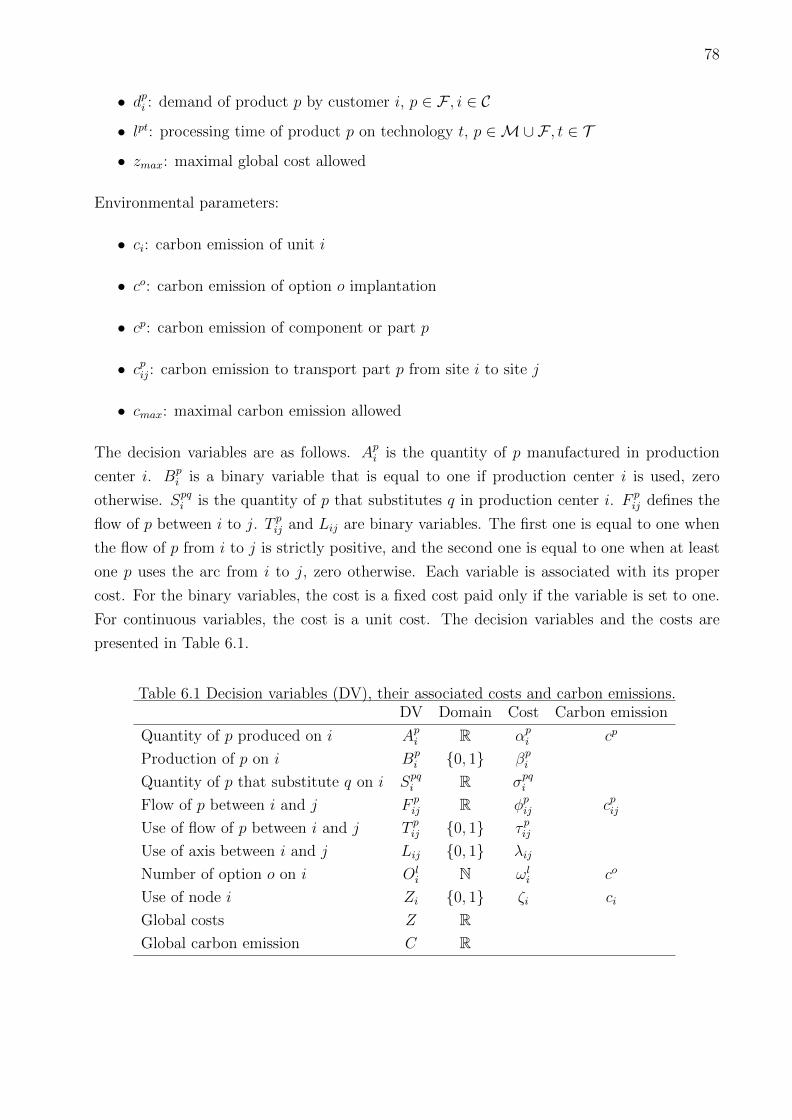
78
• dpi : demand of product p by customer i, p ∈ F , i ∈ C
• lpt: processing time of product p on technology t, p ∈M∪F , t ∈ T
• zmax: maximal global cost allowed
Environmental parameters:
• ci: carbon emission of unit i
• co: carbon emission of option o implantation
• cp: carbon emission of component or part p
• cpij: carbon emission to transport part p from site i to site j
• cmax: maximal carbon emission allowed
The decision variables are as follows. Api is the quantity of p manufactured in production
center i. Bpi is a binary variable that is equal to one if production center i is used, zero
otherwise. Spqi is the quantity of p that substitutes q in production center i. F p
ij defines the
flow of p between i to j. T pij and Lij are binary variables. The first one is equal to one when
the flow of p from i to j is strictly positive, and the second one is equal to one when at least
one p uses the arc from i to j, zero otherwise. Each variable is associated with its proper
cost. For the binary variables, the cost is a fixed cost paid only if the variable is set to one.
For continuous variables, the cost is a unit cost. The decision variables and the costs are
presented in Table 6.1.
Table 6.1 Decision variables (DV), their associated costs and carbon emissions.DV Domain Cost Carbon emission
Quantity of p produced on i Api R αp
i cp
Production of p on i Bpi {0, 1} βp
i
Quantity of p that substitute q on i Spqi R σpq
i
Flow of p between i and j F pij R φp
ij cpijUse of flow of p between i and j T p
ij {0, 1} τ pijUse of axis between i and j Lij {0, 1} λij
Number of option o on i Oli N ωl
i co
Use of node i Zi {0, 1} ζi ci
Global costs Z RGlobal carbon emission C R
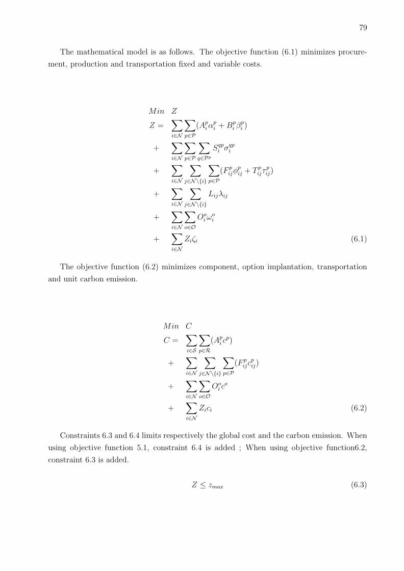
79
The mathematical model is as follows. The objective function (6.1) minimizes procure-
ment, production and transportation fixed and variable costs.
Min Z
Z =∑i∈N
∑p∈P
(Apiα
pi +Bp
i βpi )
+∑i∈N
∑p∈P
∑q∈Pp
Sqpi σ
qpi
+∑i∈N
∑j∈N\{i}
∑p∈P
(F pijφ
pij + T p
ijτpij)
+∑i∈N
∑j∈N\{i}
Lijλij
+∑i∈N
∑o∈O
Ooiω
oi
+∑i∈N
Ziζi (6.1)
The objective function (6.2) minimizes component, option implantation, transportation
and unit carbon emission.
Min C
C =∑i∈S
∑p∈R
(Api c
p)
+∑i∈N
∑j∈N\{i}
∑p∈P
(F pijc
pij)
+∑i∈N
∑o∈O
Ooi c
o
+∑i∈N
Zici (6.2)
Constraints 6.3 and 6.4 limits respectively the global cost and the carbon emission. When
using objective function 5.1, constraint 6.4 is added ; When using objective function6.2,
constraint 6.3 is added.
Z ≤ zmax (6.3)
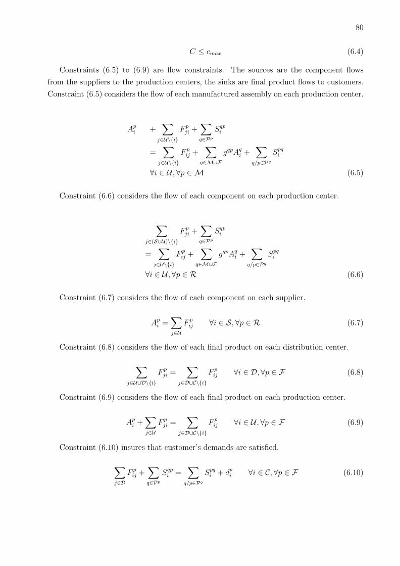
80
C ≤ cmax (6.4)
Constraints (6.5) to (6.9) are flow constraints. The sources are the component flows
from the suppliers to the production centers, the sinks are final product flows to customers.
Constraint (6.5) considers the flow of each manufactured assembly on each production center.
Api +
∑j∈U\{i}
F pji +
∑q∈Pp
Sqpi
=∑
j∈U\{i}
F pij +
∑q∈M∪F
gqpAqi +
∑q/p∈Pq
Spqi
∀i ∈ U ,∀p ∈M (6.5)
Constraint (6.6) considers the flow of each component on each production center.
∑j∈(S∪U)\{i}
F pji +
∑q∈Pp
Sqpi
=∑
j∈U\{i}
F pij +
∑q∈M∪F
gqpAqi +
∑q/p∈Pq
Spqi
∀i ∈ U ,∀p ∈ R (6.6)
Constraint (6.7) considers the flow of each component on each supplier.
Api =
∑j∈U
F pij ∀i ∈ S,∀p ∈ R (6.7)
Constraint (6.8) considers the flow of each final product on each distribution center.
∑j∈U∪D\{i}
F pji =
∑j∈D∪C\{i}
F pij ∀i ∈ D,∀p ∈ F (6.8)
Constraint (6.9) considers the flow of each final product on each production center.
Api +
∑j∈U
F pji =
∑j∈D∪C\{i}
F pij ∀i ∈ U ,∀p ∈ F (6.9)
Constraint (6.10) insures that customer’s demands are satisfied.
∑j∈D
F pij +
∑q∈Pp
Sqpi =
∑q/p∈Pq
Spqi + dpi ∀i ∈ C,∀p ∈ F (6.10)
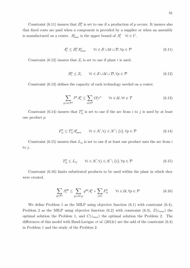
81
Constraint (6.11) insures that Bpi is set to one if a production of p occurs. It insures also
that fixed costs are paid when a component is provided by a supplier or when an assembly
is manufactured on a center. Apmax is the upper bound of Ap
i ∀i ∈ U .
Api ≤ Bp
iApmax ∀i ∈ S ∪ U ∪ D, ∀p ∈ P (6.11)
Constraint (6.12) insures that Zi is set to one if plant i is used.
Bpi ≤ Zi ∀i ∈ S ∪ U ∪ D,∀p ∈ P (6.12)
Constraint (6.13) defines the capacity of each technology needed on a center.
∑p/u∈Pp
lptApi ≤
∑o∈Ot
Ooi c
o ∀i ∈ U ,∀t ∈ T (6.13)
Constraint (6.14) insures that T pij is set to one if the arc from i to j is used by at least
one product p.
F pij ≤ T p
ijApmax ∀i ∈ N ,∀j ∈ N \ {i}, ∀p ∈ P (6.14)
Constraint (6.15) insures that Lij is set to one if at least one product uses the arc from i
to j.
T pij ≤ Lij ∀i ∈ N ,∀j ∈ N \ {i}, ∀p ∈ P (6.15)
Constraint (6.16) limits substituted products to be used within the plant in which they
were created.
∑q∈Pp
Sqpi ≤
∑q∈M\p
gqpAqi +
∑j∈C
F pij ∀i ∈ U ,∀p ∈ P (6.16)
We define Problem 1 as the MILP using objective function (6.1) with constraint (6.4),
Problem 2 as the MILP using objective function (6.2) with constraint (6.3), Z(cmax) the
optimal solution the Problem 1, and C(zmax) the optimal solution the Problem 2. The
differences of this model with Baud-Lavigne et al. (2012c) are the add of the constraint (6.4)
in Problem 1 and the study of the Problem 2.
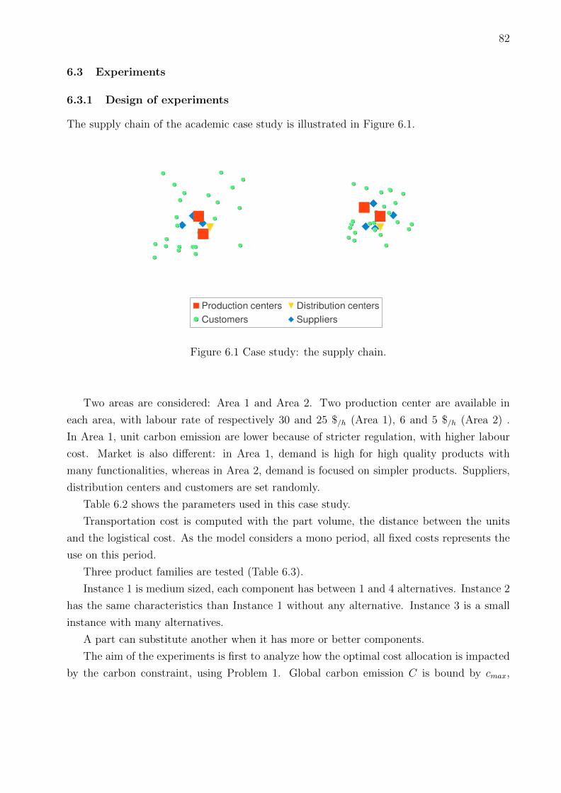
82
6.3 Experiments
6.3.1 Design of experiments
The supply chain of the academic case study is illustrated in Figure 6.1.
Production centers Distribution centers
Customers Suppliers
Figure 6.1 Case study: the supply chain.
Two areas are considered: Area 1 and Area 2. Two production center are available in
each area, with labour rate of respectively 30 and 25 $/h (Area 1), 6 and 5 $/h (Area 2) .
In Area 1, unit carbon emission are lower because of stricter regulation, with higher labour
cost. Market is also different: in Area 1, demand is high for high quality products with
many functionalities, whereas in Area 2, demand is focused on simpler products. Suppliers,
distribution centers and customers are set randomly.
Table 6.2 shows the parameters used in this case study.
Transportation cost is computed with the part volume, the distance between the units
and the logistical cost. As the model considers a mono period, all fixed costs represents the
use on this period.
Three product families are tested (Table 6.3).
Instance 1 is medium sized, each component has between 1 and 4 alternatives. Instance 2
has the same characteristics than Instance 1 without any alternative. Instance 3 is a small
instance with many alternatives.
A part can substitute another when it has more or better components.
The aim of the experiments is first to analyze how the optimal cost allocation is impacted
by the carbon constraint, using Problem 1. Global carbon emission C is bound by cmax,
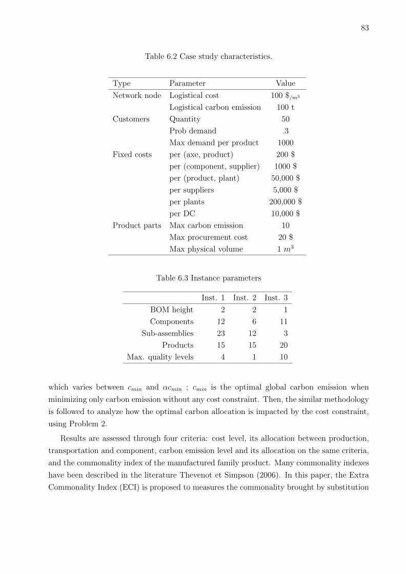
83
Table 6.2 Case study characteristics.
Type Parameter Value
Network node Logistical cost 100 $/m3
Logistical carbon emission 100 t
Customers Quantity 50
Prob demand .3
Max demand per product 1000
Fixed costs per (axe, product) 200 $
per (component, supplier) 1000 $
per (product, plant) 50,000 $
per suppliers 5,000 $
per plants 200,000 $
per DC 10,000 $
Product parts Max carbon emission 10
Max procurement cost 20 $
Max physical volume 1 m3
Table 6.3 Instance parameters
Inst. 1 Inst. 2 Inst. 3
BOM height 2 2 1
Components 12 6 11
Sub-assemblies 23 12 3
Products 15 15 20
Max. quality levels 4 1 10
which varies between cmin and αcmin ; cmin is the optimal global carbon emission when
minimizing only carbon emission without any cost constraint. Then, the similar methodology
is followed to analyze how the optimal carbon allocation is impacted by the cost constraint,
using Problem 2.
Results are assessed through four criteria: cost level, its allocation between production,
transportation and component, carbon emission level and its allocation on the same criteria,
and the commonality index of the manufactured family product. Many commonality indexes
have been described in the literature Thevenot et Simpson (2006). In this paper, the Extra
Commonality Index (ECI) is proposed to measures the commonality brought by substitution
84
decisions. ECI is computed as following:
ECI = 1− # parts used−# parts min
# parts max−# parts min
Parts contain components, high level assemblies and final products. The minimum number of
parts (# parts min) refers to the solution with a unique final product, which contains all the
components at a high quality level: it can substitute every other products. The maximum
number of parts (# parts max) refers to the number of part in the initial BOM: there is no
reason to produce other type of parts. ECI is between 0 (no extra commonality) and 1 (total
commonality) and can differ because of substitution possibilities. First, additional compo-
nents can be added to the sub-assemblies to increase standardization. Then, components can
be substituted for lower carbon impact one – or higher quality one –, to have a lower carbon
impact – or also to increase standardization. Initial commonality does not affect ECI.
Experiments are followed by solving the MILP presented in Section 6.2 with ILOG CPLEX
12 Java libraries on a server under 64 bits OS with a 2.27 GHz Intel Xeon CPU with 8 cores
and 8GB of memory.
6.3.2 Cost function minimization with carbon emission constraint
Carbon emission constraint (constraint (6.4)) is added to analyze the cost structure which
has to be found to respect a global carbon emission limit. This limit Cmax = αCmin is tested
for α ∈ [1, 3.5]. When α = 1, resolving Problem 1 is the same than resolving Problem 2
without any cost constraint. When αCmin ≥ C(Z(∞)), the carbon constraint is relaxed.
Figure 6.2 presents the Extra Commonality Index according to Cmax variation. On
the three tested instances, ECI increases with alpha. When the carbon constraint is tight,
commonality is lower when more carbon emission is authorized.
Figures 6.3 present the cost allocation on the three instances according to Cmax variation.
Carbon emission allocation is not relevant, as it has not been optimized.
On instance 1, carbon emission constraint have little impact on cost. Optimal cost is
reached when alpha is above 1.35. Under 1.35, gain is obtained mainly through transport
reduction and some product cost variation. Instance 2 is more impacted by this constraint.
When relaxing the constraint by 50%, cost can decrease by 30%. When alpha is under 1.7,
gain is from transportation and product. Above 1.7, transportation continues to decrease
while costs from components increase a little. Cost is optimal when alpha is above 2.9. On
instance 3, three stages are visible. When alpha is under 1.1, global cost is high because
of components, whose cost decrease by 30%, while transportation and production costs are
stable. Between 1.1 and 1.9, the cost gradually decreases, mainly through component cost.
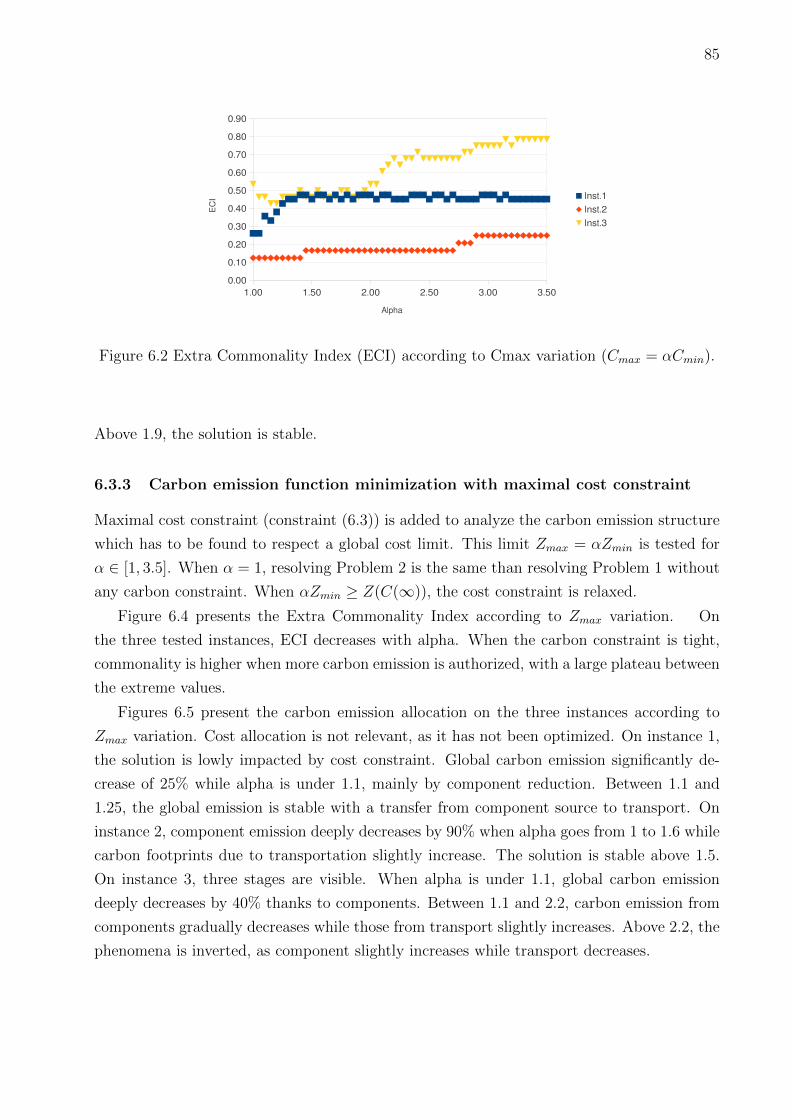
85
1.00 1.50 2.00 2.50 3.00 3.50
0.00
0.10
0.20
0.30
0.40
0.50
0.60
0.70
0.80
0.90
Inst.1
Inst.2
Inst.3
Alpha
EC
I
Figure 6.2 Extra Commonality Index (ECI) according to Cmax variation (Cmax = αCmin).
Above 1.9, the solution is stable.
6.3.3 Carbon emission function minimization with maximal cost constraint
Maximal cost constraint (constraint (6.3)) is added to analyze the carbon emission structure
which has to be found to respect a global cost limit. This limit Zmax = αZmin is tested for
α ∈ [1, 3.5]. When α = 1, resolving Problem 2 is the same than resolving Problem 1 without
any carbon constraint. When αZmin ≥ Z(C(∞)), the cost constraint is relaxed.
Figure 6.4 presents the Extra Commonality Index according to Zmax variation. On
the three tested instances, ECI decreases with alpha. When the carbon constraint is tight,
commonality is higher when more carbon emission is authorized, with a large plateau between
the extreme values.
Figures 6.5 present the carbon emission allocation on the three instances according to
Zmax variation. Cost allocation is not relevant, as it has not been optimized. On instance 1,
the solution is lowly impacted by cost constraint. Global carbon emission significantly de-
crease of 25% while alpha is under 1.1, mainly by component reduction. Between 1.1 and
1.25, the global emission is stable with a transfer from component source to transport. On
instance 2, component emission deeply decreases by 90% when alpha goes from 1 to 1.6 while
carbon footprints due to transportation slightly increase. The solution is stable above 1.5.
On instance 3, three stages are visible. When alpha is under 1.1, global carbon emission
deeply decreases by 40% thanks to components. Between 1.1 and 2.2, carbon emission from
components gradually decreases while those from transport slightly increases. Above 2.2, the
phenomena is inverted, as component slightly increases while transport decreases.
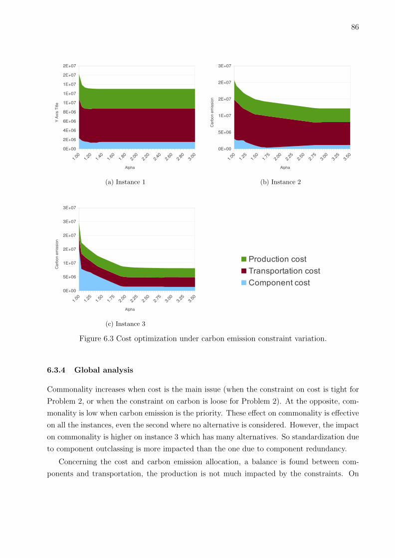
86
1.00
1.20
1.40
1.60
1.80
2.00
2.20
2.40
2.60
2.80
3.00
0E+00
2E+06
4E+06
6E+06
8E+06
1E+07
1E+07
1E+07
2E+07
2E+07
Alpha
Y A
xis
Titl
e
(a) Instance 1
1.00
1.25
1.50
1.75
2.00
2.25
2.50
2.75
3.00
3.25
3.50
0E+00
5E+06
1E+07
2E+07
2E+07
3E+07
Alpha
Carb
on e
mis
sio
n
(b) Instance 2
1.00
1.25
1.50
1.75
2.00
2.25
2.50
2.75
3.00
3.25
3.50
0E+00
5E+06
1E+07
2E+07
2E+07
3E+07
3E+07
Alpha
Carb
on e
mis
sio
n
(c) Instance 3
Figure 6.3 Cost optimization under carbon emission constraint variation.
6.3.4 Global analysis
Commonality increases when cost is the main issue (when the constraint on cost is tight for
Problem 2, or when the constraint on carbon is loose for Problem 2). At the opposite, com-
monality is low when carbon emission is the priority. These effect on commonality is effective
on all the instances, even the second where no alternative is considered. However, the impact
on commonality is higher on instance 3 which has many alternatives. So standardization due
to component outclassing is more impacted than the one due to component redundancy.
Concerning the cost and carbon emission allocation, a balance is found between com-
ponents and transportation, the production is not much impacted by the constraints. On
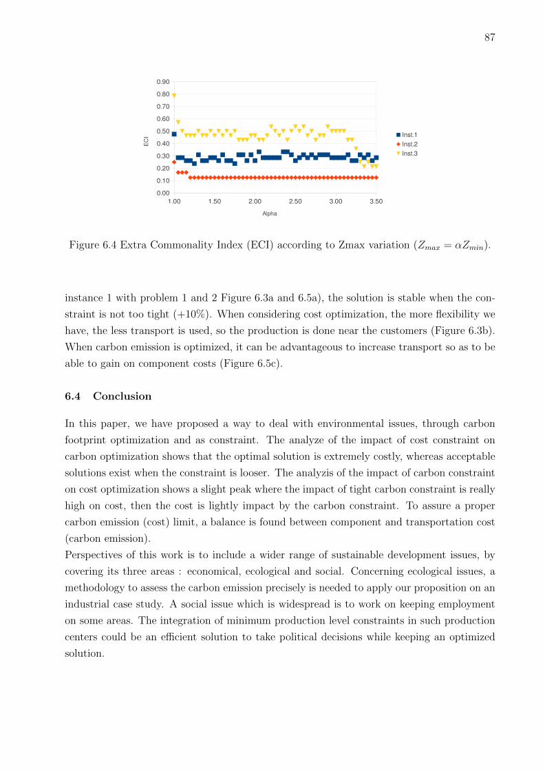
87
1.00 1.50 2.00 2.50 3.00 3.50
0.00
0.10
0.20
0.30
0.40
0.50
0.60
0.70
0.80
0.90
Inst.1
Inst.2
Inst.3
Alpha
EC
I
Figure 6.4 Extra Commonality Index (ECI) according to Zmax variation (Zmax = αZmin).
instance 1 with problem 1 and 2 Figure 6.3a and 6.5a), the solution is stable when the con-
straint is not too tight (+10%). When considering cost optimization, the more flexibility we
have, the less transport is used, so the production is done near the customers (Figure 6.3b).
When carbon emission is optimized, it can be advantageous to increase transport so as to be
able to gain on component costs (Figure 6.5c).
6.4 Conclusion
In this paper, we have proposed a way to deal with environmental issues, through carbon
footprint optimization and as constraint. The analyze of the impact of cost constraint on
carbon optimization shows that the optimal solution is extremely costly, whereas acceptable
solutions exist when the constraint is looser. The analyzis of the impact of carbon constraint
on cost optimization shows a slight peak where the impact of tight carbon constraint is really
high on cost, then the cost is lightly impact by the carbon constraint. To assure a proper
carbon emission (cost) limit, a balance is found between component and transportation cost
(carbon emission).
Perspectives of this work is to include a wider range of sustainable development issues, by
covering its three areas : economical, ecological and social. Concerning ecological issues, a
methodology to assess the carbon emission precisely is needed to apply our proposition on an
industrial case study. A social issue which is widespread is to work on keeping employment
on some areas. The integration of minimum production level constraints in such production
centers could be an efficient solution to take political decisions while keeping an optimized
solution.
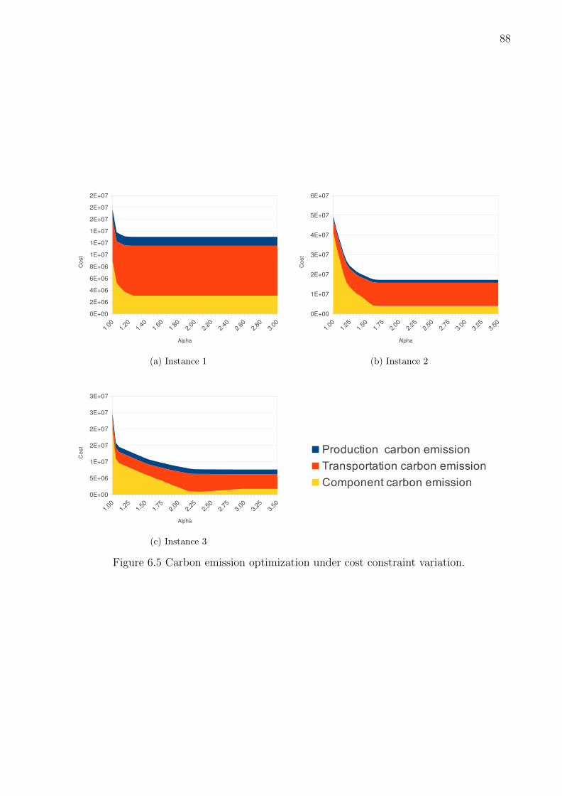
88
1.00
1.20
1.40
1.60
1.80
2.00
2.20
2.40
2.60
2.80
3.00
0E+00
2E+06
4E+06
6E+06
8E+06
1E+07
1E+07
1E+07
2E+07
2E+07
2E+07
Alpha
Cost
(a) Instance 1
1.00
1.25
1.50
1.75
2.00
2.25
2.50
2.75
3.00
3.25
3.50
0E+00
1E+07
2E+07
3E+07
4E+07
5E+07
6E+07
Alpha
Cost
(b) Instance 2
1.00
1.25
1.50
1.75
2.00
2.25
2.50
2.75
3.00
3.25
3.50
0E+00
5E+06
1E+07
2E+07
2E+07
3E+07
3E+07
Alpha
Cos
t
(c) Instance 3
Figure 6.5 Carbon emission optimization under cost constraint variation.
89
Troisieme partie
CONCLUSION GENERALE

91
CHAPITRE 7
CONCLUSION
Au cours de ce travail de these, nous nous sommes interesses a trouver une facon pertinente
de lier la conception des produits et la conception de la chaıne logistique au sein d’entreprises
manufacturieres.
Dans le Chapitre 1, nous avons positionne le probleme. Celui-ci fait appel principalement
aux travaux lies a l’optimisation des reseaux logistiques, en integrant une partie des decisions
concernant la conception des produits pouvant etre prises en phase d’industrialisation. Ces
deux domaines d’etude ainsi que les enjeux de l’etude sont explicites afin de positionner le
probleme.
Nous avons presente dans le Chapitre 2 un etat des lieux des travaux sur les liens entre
conception produits et conception de la chaıne logistique. Si cette problematique a attire un
certain nombre de travaux, le besoin d’un modele d’optimisation de conception conjointe a
ete mis en evidence. La problematique de la prise en compte des aspects environnementaux a
ete abordee, en montrant d’une part qu’il est important de considerer tout le cycle de vie des
produits, et d’autre part comment ces aspects ont ete utilises dans la conception des chaınes
logistiques.
Les objectifs que nous nous sommes fixes durant ce travail ainsi que nos hypotheses ont
ete presentes dans le Chapitre 3. Nous nous interessons particulierement aux cas de person-
nalisation de masse dans des reseaux logistiques globalises, pour lesquels les gains potentiels
peuvent etre important. Les decisions concernant la conception des produits se limitent a
des choix de substitution, qui englobent plusieurs realites : la standardisation de produits,
la definition de gammes alternatives et l’externalisation. Au niveau de la chaıne logistique,
nous considerons les decisions de localisation des sites (de production et de distribution),
d’allocation des produits dans le reseau logistique, l’implantation de moyens de production
et la selection des fournisseurs.
Nos contributions ont ete exposees sous forme d’articles qui presentent notre demarche
de facon coherente.
Notre premiere contribution a ete de justifier le besoin de modeles d’optimisation conjointe.
Nous avons montre dans le Chapitre 4 que les processus de creation de l’offre et de realisation
de l’offre, qui sont habituellement sequentiels, sont en realite interdependants. Notamment,
nous montrons par un contre-exemple sur un modele generique que des gains sont possibles
grace a l’optimisation simultanee des deux processus. Sur un cas d’etude pouvant etre resolu
92
sans modele d’optimisation, la complexite des solutions de ce type de modele a ete mise en
evidence.
Nous avons donc modelise le probleme d’optimisation conjointe produits – chaıne logis-
tique et presente des methodes de resolution dans le Chapitre 5. Apres avoir etudie les limites
de la resolution avec un solveur commercial, nous avons identifie les variables difficiles du mo-
dele, principalement les variables binaires. Nous avons developpe deux heuristiques basees sur
l’arrondie des solutions de la relaxation lineaire donnant des solutions de bonnes qualites et
permettant une reduction importante du temps d’execution, notamment sur les grosses ins-
tances, pour lesquelles les solveurs commerciaux ne peuvent pas trouver de resultat. Notre
apport a egalement ete de developper un generateur d’instance pour la chaıne logistique,
et surtout pour les familles de produits. La particularite de ce generateur est de permettre
d’avoir des instances de produits de grandes tailles en maıtrisant la plupart des parametres
definissant une famille de produits (hauteur et largeur de nomenclature, commonalite entre
les produits . . . ) tout en connaissant les possibilites de substitution.
Pour finir, le Chapitre 6 presente une analyse de la prise en compte de contraintes en-
vironnementales dans le modele que nous proposons. Ces contraintes sont integrees via les
emissions carbones des composants, des sites de production et des installations et enfin du
transport. Deux methodes sont employees pour analyser l’impact de ces contraintes : l’opti-
misation des couts avec une limitation plus ou moins importantes des emissions carbones, et
l’optimisation des emissions carbones sous contraintes de cout.
93
CHAPITRE 8
DISCUSSION ET PERSPECTIVES
La demarche suivie dans cette these a permis de faire emerger un certain nombre de pistes de
recherche et d’en approfondir une partie. Dans la continuite directe de ce travail, les autres
pistes qui nous paraissent importantes a traiter sont presentees ci-apres.
Limites et ameliorations des propositions
Le modele que nous avons propose en Chapitre 5 a ete developpe de maniere a etre utilisation
facilement en industrie. Cependant, quelques ameliorations peuvent etre apportees afin de
mieux prendre en compte les differentes realites industrielles :
• L’integration explicite des taux de change et des taxes entre les differents pays ;
• Le choix de differents modes de transport ;
• La prise en compte des delais de transport, d’approvisionnement, de fabrication ;
• La gestion de different niveaux de qualite selon les sites de production et des compo-
sants ;
• Les stocks intermediaires. La multiplication des sites de production et des etapes de
transport engendre des stocks dont le cout peut etre evaluer afin de prendre en compte
le cout des immobilisations ;
• Une chaıne logistique plus flexible. Si le reseau logistique entre les sites de production
est generique, la structure de la chaıne globale est imposee (fournisseurs - production -
distribution - clients) ;
• Des methodes de resolution exactes performantes. Actuellement, nous sommes capables
de resoudre des instances de l’ordre d’une quinzaine de sites de production avec une
famille de produits d’une centaine d’assemblage en quelques heures.
Approche globale du developpement durable
Les aspects produits et logistiques ont tous deux un impact fort sur les trois composantes –
economique, ecologique et societale – du developpement durable. Nous avons explore partiel-
lement deux facettes de celui-ci dans le Chapitre 6 : l’optimisation des couts de production
94
et d’acheminement et l’optimisation de l’empreinte carbone globale de ce processus. Une ap-
proche integree prenant en compte plus d’aspects du developpement durable aurait d’une
part des applications pertinentes en milieu industriel et d’autre part fournirait des problemes
academiques interessants a etudier.
Marche des droits a polluer. Les travaux autour des emissions carbones dans l’optimi-
sation de la chaıne logistique se sont d’abord interesses a integrer cette composante
dans des modeles existants visant l’optimisation des couts, comme dans les travaux de
Chaabane et al. (2012). Pour cela, les emissions carbones sont considerees comme des
couts ou des profits provenant d’un marche des droits a polluer. En effet, les legislations
en vigueur instaurent des quotas d’emission carbone, echangeables sur un marche, vi-
sant a reguler les actions des industriels en matiere de pollution sans etre trop coercitif.
Lorsque les prix du marche sont suffisamment importants, une production polluante
aura un cout a prendre en compte, et a l’inverse une production raisonnee permettra de
vendre des droits. L’idee ici est d’avoir une demarche en avance sur les legislations, qui
ne prennent pas encore en compte l’integralite des aspects decrits dans le Chapitre 6,
comme par exemple le choix des composants ou des fournisseurs.
Optimisation multicriteres cout - impact environnemental. Une approche complemen-
taire est de ne plus seulement optimiser une fonction de cout plus ou moins complexe,
mais de chercher de bons compromis entre l’optimisation de la fonction de cout et de la
(ou les) fonction(s) environnementale(s), via une optimisation multicriteres. Celle-ci est
couramment utilisee pour l’optimisation de l’impact environnemental d’un processus,
car les differentes composantes, dont l’empreinte carbone, ne sont pas additionnables.
Cela permet une etude plus fine destinee principalement a des outils d’aide a la decision
qualitatifs.
Integration de la demande comme variable endogene. Nos travaux considerent une
demande connue et deterministe pour l’ensemble de la famille de produits et des clients.
Si un interet fort est porte sur la prise en compte des incertitudes et des risques dans les
modeles d’optimisation logistique, l’influence de l’empreinte carbone d’un produit sur
le comportement des acheteurs n’a pas ete, a notre connaissance, integree dans ce type
de modele. Deux approches sont ici possibles. La premiere est de determiner a la fois
la famille de produits et sa chaıne logistique, comme l’ont fait Lamothe et al. (2006)
sans prendre en compte les impacts environnementaux. La seconde est de garder une ap-
proche proche de celle decrite en Section 3.2.2, en considerant que la famille de produits
a ete concue, l’inconnue restant la maniere dont ces produits vont etre fabriques. Selon
les choix de production (localisation, transport, composants . . . ), l’empreinte carbone
95
des produits varie et peut avoir un impact sur les choix des consommateurs. Une ten-
dance actuelle est en effet d’indiquer aux acheteurs des informations environnementales
du produit, telles que la consommation (en energie, en eau . . . ), le lieu de production ou
l’empreinte carbone. Il serait alors pertinent de considerer ces choix dans les decisions
de production en anticipant les impacts de ces facteurs sur les variations de demande.
Influence ethique des choix d’implantation de la production. Les impacts societaux
des decisions de localisation de la production sont difficiles a evaluer quantitativement,
mais restent neanmoins tres important sur l’image d’une entreprise et dans les compor-
tements des consommateurs. Par exemple, l’entreprise suedoise Ikea essaie de produire
dans chaque pays ou elle implante un magasin. Il est alors important de garder de la
flexibilite dans ces contraintes afin de garder des marges de manœuvre. Une premiere
approche est de contraindre un niveau de production minimal dans certains pays ou
zones geographiques, afin de donner un signal fort aux clients, ou de ne pas bouleverser
les choix d’implantation precedents. Une etude des impacts de ce type de contraintes a
ete presentee par Baud-Lavigne et al. (2011a).
Determination de nomenclatures uniques
Le modele propose dans le Chapitre 5 permet d’integrer les choix de substitutions a un
modele d’optimisation logistique sans avoir un impact significatif sur sa complexite. Pour
cela, les nomenclatures des produits ne sont pas contraintes et peuvent, pour un produit
donne, differer d’un site a l’autre, voire sur le meme site de production. Si cela permet une
solution optimale du point de vue de la fonction de cout utilisee, des consequences difficilement
quantifiables sont a prendre en compte : reactions des consommateurs si deux produits a
priori identiques different de part leurs composants, lourdeur en production pour prendre en
compte la multiplicite des modes operatoires, et difficulte de la gestion du service apres-vente.
Il parait alors pertinent de contraindre les choix de production a une seule nomenclature par
produit, de facon globale, par zone de commercialisation, ou par site de production.
Pour garder un modele lineaire, une premiere approche serait d’ajouter des variables de
decision plus precises, decrivant a quoi vont servir les substitutions, telles que presentees par
Chen (2010).
Une seconde approche serait de generer un ensemble de nomenclatures possibles et d’ajou-
ter des variables de decision booleennes determinant les nomenclatures retenues en produc-
tion, afin de pouvoir rajouter des contraintes sur le nombre de nomenclatures de production
par produit. Du fait du nombre exponentiel de nomenclatures a generer, il n’est pas possible
d’enumerer et d’ajouter au modele toutes les possibilites. Un des enjeux est de determiner
96
quelles nomenclatures sont a priori interessantes. Une resolution en deux phases (generation
des nomenclatures, puis optimisation) est permise par cette methode iterative : apres une
premiere resolution, il est possible de rajouter des nomenclatures pertinentes au modele pour
ameliorer la solution. Une methode de resolution basee sur la generation de colonnes semble
alors bien adaptee a ce type de modele.
Prise en compte des cycles de vie des produits en production
Nous nous sommes concentres dans ces travaux sur des modeles mono-periodes, considerant
une demande stable sur une periode donnee. Or, le cycle de vie d’une famille de produits
possede des phases de montee en charge, de declin et de renouvellement qui different pour
chaque produit de la famille. Plusieurs aspects sont a prendre en compte :
• la plupart du temps, seuls quelques produits sont lances au debut, afin de diminuer
les risques (en production et commercialement). La gamme est ensuite elargie petit a
petit ;
• pour un produit donne, les volumes de production ne sont pas constant durant son
cycle de vie : montee en charge en debut de vie, declin progressif en fin de vie ;
• le renouvellement des produits en fin de vie peut impliquer que plusieurs produits
proches se chevauchent en production.
Les aspects predominants sont alors d’ordre tactique : comment adapter la fabrication a
ces variations anticipees de production ? En considerant un modele multi-periodes, les deci-
sions de reallocation des moyens de production et d’adaptation des produits prennent tout
leur sens.
97
REFERENCES
AGARD, B., DA CUNHA, C. et CHEUNG, B. (2009). Composition of module stock for
final assembly using an enhanced genetic algorithm. International Journal of Production
Research, 47, 5829–5842.
AGARD, B. et KUSIAK, A. (2004). Data mining for subassembly selection. Journal of
Manufacturing Science and Engineering, 126, 627–631.
AGARD, B. et PENZ, B. (2009). A simulated annealing method based on a clustering
approach to determine bills of materials for a large product family. International Journal of
Production Economics, 117, 389–401.
APPELQVIST, P., LEHTONEN, J. et KOKKONEN, J. (2004). Modelling in product and
supply chain design : literature survey and case study. Journal of Manufacturing Technology
Management, 15, 675 – 686.
ARNTZEN, B. C., BROWN, G. G., HARRISON, T. P. et TRAFTON, L. L. (1995). Global
supply chain management at digital equipment corporation. Interfaces, 25, 69–93.
BARAJAS, M. et AGARD, B. (2009). Fuzzy product configuration based on market seg-
mentation to form a family of products. 42nd CIRP Conference on Manufacturing Systems.
Grenoble, France.
BASSETT, M. et GARDNER, L. (2010). Designing optimal global supply chains at dow
AgroSciences. Annals of Operations Research, doi : 10.1007/s10479-010-0802-2.
BAUD-LAVIGNE, B., AGARD, B. et PENZ, B. (2010). Impact de la standardisation
sur la conception integree d’une chaıne logistique dans un contexte d’internationalisation.
Proceedings of 8eme Conference Francophone de MOdelisation et SIMulation-MOSIM.
Hammamet, Tunisie.
BAUD-LAVIGNE, B., AGARD, B. et PENZ, B. (2011a). Impacts of minimum activity
level and multi-sourcing on product family and supply chain design. T. K. Dieter Spath,
Rolf Ilg, editeur, International Conference on Production Research (ICPR 21) : Innovation
in Product and Production July 31 - August 4, 2011 in Stuttgart, Germany ; Confernce
Proceedings. Fraunhofer Verlag, Stuttgart, Allemagne, CD–rom. ISBN 978-3-8396-0293-5
OSP OSP.
98
BAUD-LAVIGNE, B., AGARD, B. et PENZ, B. (2011b). A MILP model for joint product
family and supply chain design. Proceedings of the International Conference on Industrial
Engineering and Systems Management (IESM’2011). International Institute for Innovation,
Industrial Engineering and Entrepreneurship (I4e2), Metz, France, 889 – 897. ISBN 978-2-
9600532-3-4.
BAUD-LAVIGNE, B., AGARD, B. et PENZ, B. (2011c). Un nouveau modele pour la
conception conjointe d’une famille de produits et de sa chaıne logistique avec standardisation,
externalisation et gammes alternatives. Congres International de Genie Industriel. Saint-
Sauveur, Canada, CD–rom. OSP OSP.
BAUD-LAVIGNE, B., AGARD, B. et PENZ, B. (2012a). Environmental constraints in
joint product and supply chain design optimization. Soumis a Computers & Industrial
Engineering.
BAUD-LAVIGNE, B., AGARD, B. et PENZ, B. (2012b). Mutual impacts of product stan-
dardization and supply chain design. International Journal of Production Economics, 135,
50–60.
BAUD-LAVIGNE, B., AGARD, B. et PENZ, B. (2012c). Simultaneous product family
and supply chain design : An optimization approach. Soumis a International Journal of
Production Economics.
BEAMON, B. (2005). Environmental and sustainability ethics in supply chain management.
Science and Engineering Ethics, 11, 221–234.
BEAMON, B. M. (1999a). Designing the green supply chain. Logistics Information
Management, 12, 332 – 342.
BEAMON, B. M. (1999b). Measuring supply chain performance. International Journal of
Operations & Production Management, 19, 275 – 292.
BOUCHRIHA, H. (2002). Faire ou faire-faire dans la conception d’une machine logistique
: un outil d’aide a la decision. These de doctorat, Institut National Polytechnique de
Grenoble, France.
BREZET, H. et HEMEL, C. V. (1997). EcoDesign : A Promising Approach to Sustainable
Production and Consumption. United Nations Environment Programme, Industry and En-
vironment, Cleaner Production.
99
BRIANT, O. et NADDEF, D. (2004). The optimal diversity management problem.
Operations Research, 52, 515–526.
CAKIR, O. (2009). Benders decomposition applied to multi-commodity, multi-mode distri-
bution planning. Expert Systems with Applications, 36, 8212–8217.
CAMUFFO, A., FURLAN, A., ROMANO, P. et VINELLI, A. (2006). The process of supply
network internationalisation. Journal of Purchasing and Supply Management, 12, 135–147.
CHAABANE, A., RAMUDHIN, A. et PAQUET, M. (2009). Designing supply chains
with sustainability considerations. International Conference on Industrial Engineering and
Systems Management. Montreal, Canada.
CHAABANE, A., RAMUDHIN, A. et PAQUET, M. (2012). Design of sustainable supply
chains under the emission trading scheme. International Journal of Production Economics,
135, 37–49.
CHAKRAVARTY, A. et BALAKRISHNAN, N. (2001). Achieving product variety through
optimal choice of module variations. IIE Transactions, 33, 587–598.
CHEN, H.-Y. (2010). The impact of item substitutions on production-distribution networks
for supply chains. Transportation Research Part E : Logistics and Transportation Review,
46, 803–819.
CHEN, H.-Y., LIN, C.-W. et YIH, Y. (2007). Production-distribution network design of
a global supply chain alliance from the key player’s perspective. International Journal of
Production Research, 45, 245–265.
CHOUMAN, M., CRAINIC, T. G. et GENDRON, B. (2009). A cutting-plane algorithm for
multicommodity capacitated fixed-charge network design. Rapport technique, CIRRELT,
Montreal.
COHEN, M. et MOON, S. (1991). An integrated plant loading model with economies of
scale and scope. European Journal of Operational Research, 50, 266–279.
COPACINO, W. C. (1997). Supply chain management : The basics and beyond. CRC
Press.
CORDEAU, J.-F., LAPORTE, G. et PASIN, F. (2008). An iterated local search heuristic
for the logistics network design problem with single assignment. International Journal of
Production Economics, 113, 626–640.
100
CORDEAU, J.-F., PASIN, F. et SOLOMON, M. (2006). An integrated model for logistics
network design. Annals of Operations Research, 144, 59–82.
DA CUNHA, C. (2004). Definition et gestion de produits semi-finis en vue d’une production
de type ’assemblage a la commande’. These de doctorat, Grenoble INP.
DA CUNHA, C., AGARD, B. et KUSIAK, A. (2007). Design for cost : Module-based mass
customization. IEEE Transactions on Automation Science and Engineering, 4, 350–359.
DAS, K. (2011). A quality integrated strategic level global supply chain model. International
Journal of Production Research, 49, 5–31.
DESAI, P., KEKRE, S., RADHAKRISHNAN, S. et SRINIVASAN, K. (2001). Product
differentiation and commonality in design : Balancing revenue and cost drivers. Management
Science, 47, 37–51.
DOGAN, K. et GOETSCHALCKX, M. (1999). A primal decomposition method for the
integrated design of multi-period production-distribution systems. IIE Transactions, 31,
1027–1036.
DOWLATSHAHI, S. (1996). The role of logistics in concurrent engineering. International
Journal of Production Economics, 44, 189–199.
DOWLATSHAHI, S. (1999). A modeling approach to logistics in concurrent engineering.
European Journal of Operational Research, 115, 59–76.
EL HADJ KHALAF, R. (2009). Definition des nomenclatures et des sources
d’approvisionnement pour la fabrication d’une famille de produits. These de doctorat,
Grenoble INP.
EL HADJ KHALAF, R., AGARD, B. et PENZ, B. (2010). An experimental study for the
selection of modules and facilities in a mass customization context. Journal of Intelligent
Manufacturing, 21, 703–716.
EL HADJ KHALAF, R., AGARD, B. et PENZ, B. (2011). Module selection and supply
chain optimization for customized product families using redundancy and standardization.
IEEE Transactions on Automation Science and Engineering, 8, 118–129.
ELMARAGHY, H. et MAHMOUDI, N. (2009). Concurrent design of product modules struc-
ture and global supply chain configurations. International Journal of Computer Integrated
Manufacturing, 22, 483–493.
101
FERDOWS, K. (1997). Making the most of foreign factories. Harvard Business Review.
FIXSON, S. K. (2007). Modularity and commonality research : Past developments and
future opportunities. Concurrent Engineering, 15, 85–111.
FOURNIER, X. et AGARD, B. (2007). Improvement of earliness and lateness by postpo-
nement on an automotive production line. International Journal of Flexible Manufacturing
Systems, 19, 107–121.
FROTA NETO, J., BLOEMHOF-RUWAARD, J., VAN NUNEN, J. et VAN HECK, E.
(2008). Designing and evaluating sustainable logistics networks. International Journal of
Production Economics, 111, 195–208.
GEOFFRION, A. M. et GRAVES, G. W. (1974). Multicommodity distribution system
design by benders decomposition. Management Science, 20, 822–844.
GUPTA, S. et KRISHNAN, V. (1999). Integrated component and supplier selection for a
product family. Production and Operations Management, 8, 163–182.
HADJ HAMOU, K. (2002). Contribution a la conception de produits a forte diversite et de
leur chaıne logistique : une approche par contraintes. These de doctorat, INP Toulouse.
HAMMAMI, R., FREIN, Y. et HADJ-ALOUANE, A. (2008). Supply chain design in the de-
localization context : Relevant features and new modeling tendencies. International Journal
of Production Economics, 113, 641–656.
HAMMAMI, R., FREIN, Y. et HADJ-ALOUANE, A. B. (2009). A strategic-tactical model
for the supply chain design in the delocalization context : Mathematical formulation and a
case study. International Journal of Production Economics, 122, 351–365.
JIAO, J., SIMPSON, T. et SIDDIQUE, Z. (2007). Product family design and platform-based
product development : a state-of-the-art review. Journal of Intelligent Manufacturing, 18,
5–29.
JOHNSON, M. et KIRCHAIN, R. (2010). Developing and assessing commonality me-
trics for product families : A process-based cost-modeling approach. IEEE Transactions
on Engineering Management, 57, 634–648.
KLIBI, W., MARTEL, A. et GUITOUNI, A. (2010). The design of robust value-creating
supply chain networks : A critical review. European Journal of Operational Research, 203,
283–293.
102
KOIKE, T. (2005). Les interfaces pour l’integration de la logistique dans les projets de
conception. une contribution basee sur le cas du projet d’un tracteur a chenille. These de
doctorat, Institut National Polytechnique de Grenoble, France.
KUSIAK, A. et HUANG, C. C. (1996). Development of modular products. IEEE
Transactions on Components, Packaging, and Manufacturing Technology, Part A, 19, 523–
538.
LAMOTHE, J., BONNAFE, A., GORGAS, M., DUPONT, L. et ALDANONDO, M.
(2008). Experimentation d’un modele de conception d’une famille de produits et de
sa chaine logistique. Proceedings of 7eme Conference Francophone de MOdelisation et
SIMulation-MOSIM. Paris, France.
LAMOTHE, J., HADJ-HAMOU, K. et ALDANONDO, M. (2006). An optimization mo-
del for selecting a product family and designing its supply chain. European Journal of
Operational Research, 169, 1030–1047.
LAU, A. K. W., YAM, R. C. M., TANG, E. P. Y. et SUN, H. Y. (2010). Factors influencing
the relationship between product modularity and supply chain integration. International
Journal of Operations & Production Management, 30, 951–977.
LEE, H. et TANG, C. (1997). Modelling the costs and benefits of delayed product differen-
tiation. Management Science, 43, 40–53.
LIANG, D. et WILHELM, W. (2008). Decomposition schemes and acceleration techniques
in application to production-assembly-distribution system design. Computers & Operations
Research, 35, 4010–4026.
LIN, J.-R., NOZICK, L. et TURNQUIST, M. (2006). Strategic design of distribution sys-
tems with economies of scale in transportation. Annals of Operations Research, 144, 161–
180.
LOWSON, R. (2001). Offshore sourcing : An optimal operational strategy ? Business
Horizons, 44, 61–66.
LUO, X., KWONG, C., TANG, J., DENG, S. et GONG, J. (2011). Integrating supplier
selection in optimal product family design. International Journal of Production Research,
49, 4195–4222.
MANSOORNEJAD, B., CHAMBOST, V. et STUART, P. (2010). Integrating product
portfolio design and supply chain design for the forest biorefinery. Computers & Chemical
Engineering, 34, 1497–1506.
103
MANZINI, R. et BINDI, F. (2009). Strategic design and operational management opti-
mization of a multi stage physical distribution system. Transportation Research Part E :
Logistics and Transportation Review, 45, 915–936.
MARTEL, A. (2005). The design of production-distribution networks : A mathematical
programming approach. Supply Chain Optimization. 265–305.
MEIXELL, M. et GARGEYA, V. (2005). Global supply chain design : A literature review
and critique. Transportation Research Part E : Logistics and Transportation Review, 41,
531–550.
MELO, M., NICKEL, S. et SALDANHA-DA-GAMA, F. (2006). Dynamic multi-commodity
capacitated facility location : a mathematical modeling framework for strategic supply chain
planning. Computers & Operations Research, 33, 181–208.
MELO, M., NICKEL, S. et SALDANHA-DA-GAMA, F. (2009). Facility location and supply
chain management - a review. European Journal of Operational Research, 196, 401–412.
MOHAMMADI BIDHANDI, H. et MOHD YUSUFF, R. (2011). Integrated supply chain
planning under uncertainty using an improved stochastic approach. Applied Mathematical
Modelling, 35, 2618–2630.
MOHAMMADI BIDHANDI, H., MOHD YUSUFF, R., MEGAT AHMAD, M. et ABU BA-
KAR, M. (2009). Development of a new approach for deterministic supply chain network
design. European Journal of Operational Research, 198, 121–128.
MONTREUIL, B. et POULIN, M. (2005). Demand and supply network design scope for
personalized manufacturing. Production Planning & Control, 16, 454 – 469.
NARAHARISETTI, P., KARIMI, I. et SRINIVASAN, R. (2008). Supply chain rede-
sign through optimal asset management and capital budgeting. Computers & Chemical
Engineering, 32, 3153–3169.
NEPAL, B., MONPLAISIR, L. et FAMUYIWA, O. (2012). Matching product architecture
with supply chain design. European Journal of Operational Research, 216, 312–325.
PAQUET, M. (2007). Optimisation de l’ingenierie de reseaux manufacturiers. These de
doctorat, Universite Laval.
PAQUET, M., MARTEL, A. et DESAULNIERS, G. (2004). Including technology selec-
tion decisions in manufacturing network design models. International Journal of Computer
Integrated Manufacturing, 17, 117–125.
104
PAQUET, M., MARTEL, A. et MONTREUIL, B. (2008). A manufacturing network design
model based on processor and worker capabilities. International Journal of Production
Research, 46, 2009–2030.
PEIDRO, D., MULA, J., POLER, R. et LARIO, F. (2009). Quantitative models for sup-
ply chain planning under uncertainty : a review. The International Journal of Advanced
Manufacturing Technology, 43, 400–420.
PINE, B. J. (1993). Mass customization : The new frontier in business competition. Harvard
business school press.
PIRARD, F. (2005). Une demarche hybride d’aide a la decision pour la reconfiguration
et la planification strategique des reseaux logistiques des entreprises multi-sites. These de
doctorat, Facultes universitaires catholiques de Mons.
POULIN, M., MONTREUIL, B. et MARTEL, A. (2006). Implications of personalization
offers on demand and supply network design : A case from the golf club industry. European
Journal of Operational Research, 169, 996–1009.
RAMDAS, K. et RANDALL, T. (2008). Does component sharing help or hurt reliability ?
an empirical study in the automotive industry. Management Science, 54, 922–938.
RIOPEL, D., LANGEVIN, A. et CAMPBELL, J. (2005). The network of logistics decisions.
Logistics Systems : Design and Optimization, Springer US. 1–38.
RIOPEL, D., LANGEVIN, A. et CAMPBELL, J. F. (1998). Integrating logistics in concur-
rent product and process design. Cahiers du GERAD.
ROMEIJN, H., SHU, J. et TEO, C.-P. (2007). Designing two-echelon supply networks.
European Journal of Operational Research, 178, 449–462.
SALVADOR, F., FORZA, C. et RUNGTUSANATHAM, M. (2002). Modularity, product va-
riety, production volume, and component sourcing : theorizing beyond generic prescriptions.
Journal of Operations Management, 20, 549–575.
SALVADOR, F., RUNGTUSANATHAM, M. et FORZA, C. (2004). Supply-chain configu-
rations for mass customization. Production Planning & Control, 15, 381 – 397.
SCHULZE, L. et LI, L. (2009a). Location-allocation model for logistics networks with
implementing commonality and postponement strategies. Proceedings of the International
MultiConference of Engineers and Computer Scientists, 2, 1615–1620.
105
SCHULZE, L. et LI, L. (2009b). A logistics network model for postponement supply chain.
International Journal of Applied Mathematics, 39.
SHAFIA, M. A., ARIYANEZHAD, M. G., FATHOLLAH, M. et TAHAM, F. (2009). Sup-
ply chains based on common platforms : Analysis of time savings gained by commonality.
Journal of Applied Sciences, 9, 27–37.
SHAPIRO, J. F. (2001). Modeling the supply chain. Duxbury Resource Center.
SHIMIZU, Y., FUSHIMI, H. et WADA, T. (2011). Robust logistics network modeling
and design against uncertainties. Journal of Advanced Mechanical Design, Systems, and
Manufacturing, 5, 103–114.
SIMPSON, T. W., SIDDIQUE, Z. et JIAO, J. (2006). Product platform and product family
design : methods and applications. Springer, New York.
STADZISZ, P. C. et HENRIOUD, J. M. (1998). An integrated approach for the design of
multi-product assembly systems. Computers in Industry, 36, 21–29.
SU, J. C., CHANG, Y. L. et FERGUSON, M. (2005). Evaluation of postponement structures
to accommodate mass customization. Journal of Operations Management, 23, 305–318.
TANG, J., YUNG, K.-L. et IP, A. (2004). Heuristics-based integrated decisions for logistics
network systems. Journal of Manufacturing Systems, 23, 1–13.
THANH, P. N., BOSTEL, N. et PETON, O. (2008). A dynamic model for facility location
in the design of complex supply chains. International Journal of Production Economics,
113, 678–693.
THANH, P. N., PETON, O. et BOSTEL, N. (2010). A linear relaxation-based heuristic
approach for logistics network design. Computers & Industrial Engineering, 59, 964–975.
THEVENOT, H. et SIMPSON, T. (2006). Commonality indices for assessing product fa-
milies. Product platform and product family design : methods and applications, Springer,
New York.
THONEMANN, U. W. et BRANDEAU, M. L. (2000). Optimal commonality in component
design. Operations Research, 48, 1–19.
TUKKER, A. et JANSEN, B. (2006). Environmental impacts of products : A detailed
review of studies. Journal of Industrial Ecology, 10, 159–182.
106
VERTER, V. et DASCI, A. (2002). The plant location and flexible technology acquisition
problem. European Journal of Operational Research, 136, 366–382.
VILA, D., BEAUREGARD, R. et MARTEL, A. (2005). The strategic design of forest
industry supply chains. Document de travail du CENTOR DT-2005-RB-2, Universite Laval,
Quebec, Canada.
VILA, D., MARTEL, A. et BEAUREGARD, R. (2006). Designing logistics networks in
divergent process industries : A methodology and its application to the lumber industry.
International Journal of Production Economics, 102, 358–378.
WACKER, J. et TRELEVEN, M. (1986). Component part standardization : An analysis
of commonality sources and indices. Journal of Operations Management, 6, 219–244.
WANG, F., LAI, X. et SHI, N. (2011). A multi-objective optimization for green supply
chain network design. Decision Support Systems, 51, 262–269.
YAN, H., YU, Z. et EDWIN CHENG, T. (2003). A strategic model for supply chain design
with logical constraints : formulation and solution. Computers & Operations Research, 30,
2135–2155.
ZHANG, X., HUANG, G., HUMPHREYS, P. et BOTTA-GENOULAZ, V. (2010). Simul-
taneous configuration of platform products and manufacturing supply chains : compara-
tive investigation into impacts of different supply chain coordination schemes. Production
Planning & Control, 21, 609.
ZHANG, X., HUANG, G. Q. et RUNGTUSANATHAM, M. J. (2008). Simultaneous confi-
guration of platform products and manufacturing supply chains. International Journal of
Production Research, 46, 6137–6162.
107
ANNEXE A
PARTENARIAT INDUSTRIEL AVEC REYES CONSTRUCTIONS
Contexte de l’etude
La problematique de cette these emane d’un probleme industriel de la societe Reyes Construc-
tions (RC), une PME francaise specialisee dans l’assemblage de produits electro-mecaniques.
L’entreprise possede trois sites de production situes en region Rhone-Alpes et compte environ
250 employes pour un chiffre d’affaire de 25 millions d’euros. Sa production se fait exclusi-
vement en position de sous-traitant, et se repartit entre des contrats de produits uniques ou
de petites series et des contrats de moyennes series – de l’ordre d’une dizaine de milliers de
produits au maximum.
Notre partenariat concerne l’acquisition en 2008 d’un site de production en Tunisie. Ce site
s’inscrit dans une volonte de proposer a leurs clients une offre a bas cout de main d’œuvre.
Cette decision strategique a ete prise dans le but de donner un signal important sur les
capacites de RC a proposer des services concurrentiels. Cependant, l’entreprise ne possede pas
d’expertise quant aux choix d’allocation des produits a fabriquer sur des sites de production
possedant des caracteristiques differentes et impliquant des couts logistiques importants.
Notre role est de proposer une methodologie permettant de determiner la chaıne logistique a
utiliser pour un contrat donne. La chaıne logistique de RC pour un contrat donne est definie
de facon generique en Figure A.1. Nous considerons les acteurs suivants :
Le site “local” regroupe les sites francais de l’entreprise. Ces sites ne sont pas specialises et
sont pres les uns des autres. Les clients sont proches du site local ;
Le site “distant” le site tunisien. Le cout de la main d’œuvre est plus bas, mais les couts
d’implantation d’une ligne de production sont plus eleves principalement a cause du
cout de formation ;
Les clients sont les clients finaux ou le donneur d’ordre. Le donneur d’ordre peut fournir
les composants aux sites de productions ;
Les fournisseurs peuvent etre imposes par le client ou geres par RC.
L’objectif est de pouvoir determiner l’allocation des produits aux sites de production. Le
type de solution attendue est illustre en Figure A.2.
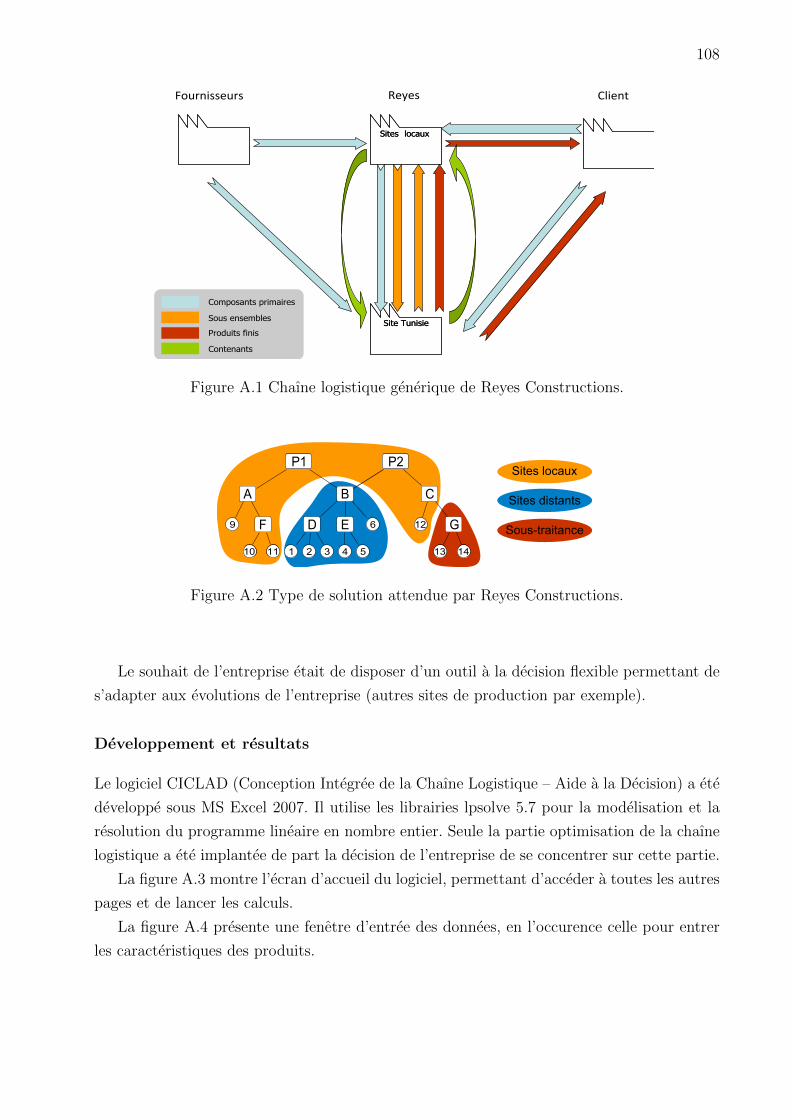
108
Sites locauxSites locaux
Site TunisieSite Tunisie
ReyesFournisseurs Client
Composants primaires
Sous ensembles
Produits finis
Contenants
Figure A.1 Chaıne logistique generique de Reyes Constructions.
Sites locaux
Sites distants
Sous-traitance
P1
A B
F D E9
1010 1011 1 2 3 4 5
6
P2
C
G12
1013 1014
Figure A.2 Type de solution attendue par Reyes Constructions.
Le souhait de l’entreprise etait de disposer d’un outil a la decision flexible permettant de
s’adapter aux evolutions de l’entreprise (autres sites de production par exemple).
Developpement et resultats
Le logiciel CICLAD (Conception Integree de la Chaıne Logistique – Aide a la Decision) a ete
developpe sous MS Excel 2007. Il utilise les librairies lpsolve 5.7 pour la modelisation et la
resolution du programme lineaire en nombre entier. Seule la partie optimisation de la chaıne
logistique a ete implantee de part la decision de l’entreprise de se concentrer sur cette partie.
La figure A.3 montre l’ecran d’accueil du logiciel, permettant d’acceder a toutes les autres
pages et de lancer les calculs.
La figure A.4 presente une fenetre d’entree des donnees, en l’occurence celle pour entrer
les caracteristiques des produits.
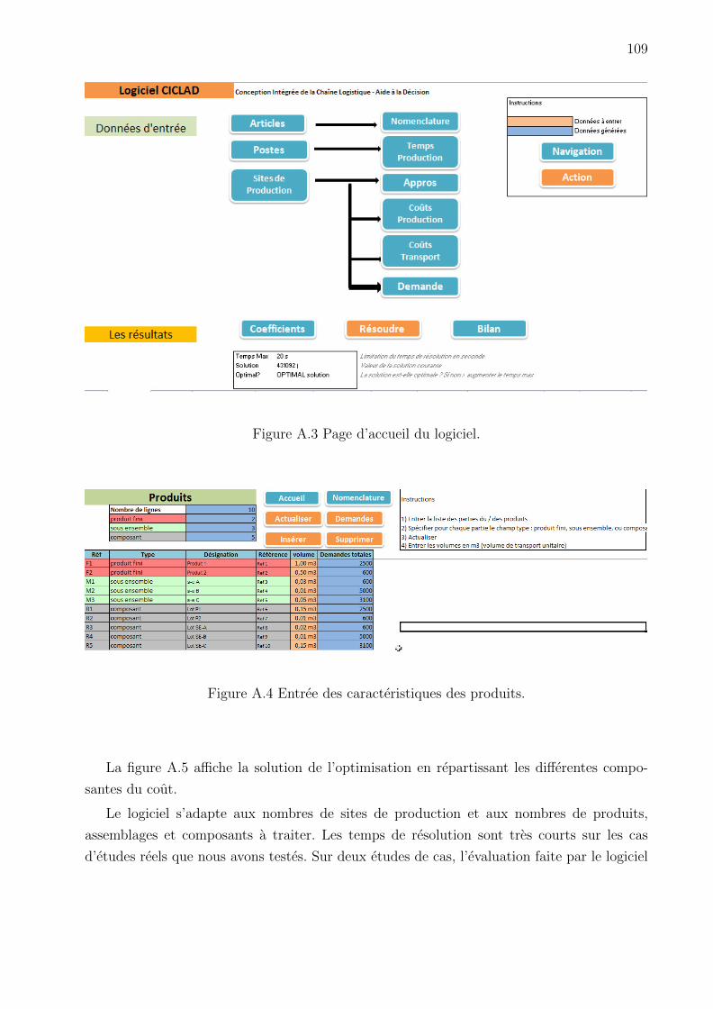
109
Figure A.3 Page d’accueil du logiciel.
Figure A.4 Entree des caracteristiques des produits.
La figure A.5 affiche la solution de l’optimisation en repartissant les differentes compo-
santes du cout.
Le logiciel s’adapte aux nombres de sites de production et aux nombres de produits,
assemblages et composants a traiter. Les temps de resolution sont tres courts sur les cas
d’etudes reels que nous avons testes. Sur deux etudes de cas, l’evaluation faite par le logiciel
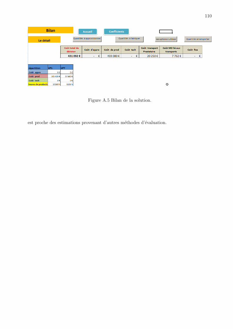
110
Figure A.5 Bilan de la solution.
est proche des estimations provenant d’autres methodes d’evaluation.

Titre Conception conjointe des nomenclatures et de la chaîne logistiquepour une famille de produits : outils d’optimisation et analyse
Résumé Le travail de thèse présenté dans ce mémoire porte sur des mé-thodes d’optimisation pour la conception conjointe des nomenclatures d’unefamille de produits et de sa chaîne logistique. Dans les milieux industrielscomme dans les services, le contexte commercial très concurrentiel oblige lesentreprises à diversifier leurs offres pour mieux répondre aux demandes deleurs clients. La gestion de cette diversité est alors une problématique cen-trale : comment proposer une large variété de produits pour satisfaire lesbesoins des clients tout en maîtrisant les coûts de production, d’inventaireet de logistique ? Les réponses à problème relèvent des disciplines habituel-lement séparées : la conception des produits, la production et la logistique.Si une majorité des approches existantes traitent ces problématiques de fa-çon séquentielle, l’interdisciplinarité apparaît cependant comme un élémentessentiel dans la gestion de la diversité. L’objectif de cette thèse est de cher-cher comment améliorer les interactions entre la conception de familles deproduits et l’optimisation des réseaux logistiques en proposant une étape deconception intermédiaire et en développant des outils mathématiques, avecun intérêt pariculier porté aux problématiques de développement durable.
Mots-clés Réseau logistique, Famille de produits, Programme linéaire ennombres mixtes, Chaîne logistique verte, Aide à la décision
Title Joint bills-of-materials and supply chain design for a product family :optimization tools and analysis
Abstract This PhD thesis addresses the problem of joint bills-of-materialsand supply chain design for a product family. In industry as well as in ser-vices, the highly competitive business environment obliges companies todiversify their offers to meet the demands of their customers. Then, mana-ging diversity is a central issue : how to offer a wide variety of products tomeet customer needs while controlling costs of production, inventory andlogistics ? Answers to theses problems are usually in separate disciplines :product design, production and logistics. If most of existing approaches ta-ckle these problems sequentially, interdisciplinarity, however, appears as akey aspect of diversity management. The objective of this thesis is to inves-tigate how to improve the interaction between product families design andsupply chain optimization and to develop mathematical tools, with a focuson sustainable development.
Keywords Supply chain design, Product family, Mixed Integer Linear Pro-gramming, Green supply chain, Decision support