Concepts and Methods of the U.S. National Income and Product Accounts

(Chapters 1–10 and 13)

November 2012

Preface The “NIPA Handbook” begins with introductory chapters that describe the fundamental concepts, definitions, classifications, and accounting framework that underlie the national income and product accounts (NIPAs) of the United States and the general sources and methods that are used to prepare the NIPA estimates. It continues with separate chapters that describe the sources and methods that are used to prepare the expenditure and income components of the accounts. The Handbook is intended to be a living reference that can be updated to reflect changes in concepts or methodology as they are introduced into the NIPAs. This release of the NIPA Handbook consists of updated versions of the first nine chapters to reflect the 2012 annual revision and of new chapters on compensation and on corporate profits. Additional chapters will be incorporated as they become available.

Acknowledgments

Douglas R. Fox, formerly of the Bureau of Economic Analysis (BEA), is leading the preparation of this Handbook. Major contributors include Stephanie H. McCulla, Eugene P. Seskin, and Shelly Smith, all of BEA’s National Income and Wealth Division (NIWD). Technical expertise has been provided by the staffs of NIWD, Balance of Payments Division, and Government Division. Brent R. Moulton, BEA’s Associate Director for National Economic Accounts, Carol E. Moylan, former Chief of NIWD, and Nicole M. Mayerhauser, Chief of NIWD, have provided overall guidance.

Table of Contents CHAPTER 1: INTRODUCTION

The U.S. national income and product accounts (NIPAs) are a set of economic accounts that provide the framework for presenting detailed measures of U.S. output and income. This chapter introduces the NIPAs by answering several basic questions about their nature and purpose.

CHAPTER 2: FUNDAMENTAL CONCEPTS

The NIPAs are based on a consistent set of concepts and definitions. This chapter establishes the type and scope of the economic activities that are covered by the NIPA measures, and it describes several of the principal NIPA measures of these activities. It then discusses the classifications used in presenting the NIPA estimates, and it describes the accounting framework that underlies the NIPAs.

CHAPTER 3: PRINCIPAL SOURCE DATA

The NIPAs incorporate a vast amount of data from a variety of public and private sources. This chapter describes the principal source data that are used to prepare the current quarterly NIPA estimates, to prepare the annual revisions of the NIPAs, and to prepare the quinquennial comprehensive revisions of the NIPAs.

CHAPTER 4: ESTIMATING METHODS

Estimating methods are the steps that are taken to transform source data into estimates that are consistent with the concepts, definitions, and framework of the NIPAs. This chapter briefly describes some of the general methods that are used to prepare the current-dollar, quantity, and price estimates for the NIPAs. An appendix describes some of the statistical tools and conventions that are used in preparing and presenting the NIPA estimates.

CHAPTER 5: PERSONAL CONSUMPTION EXPENDITURES

Personal consumption expenditures (PCE) is the NIPA measure of consumer purchases of goods and services in the U.S. economy. This chapter describes the concepts, source data, and methods that underlie the PCE estimates. A technical note provides additional detail on the methodology for a number of key PCE components.

CHAPTER 6: PRIVATE FIXED INVESMENT

Private fixed investment (PFI) is the NIPA measure of spending by private business, nonprofit institutions, and households on fixed assets in the U.S. economy. This chapter describes the concepts, source data, and methods that underlie the PFI estimates. A technical note provides additional detail on the methodology for several key PFI components.

CHAPTER 7: CHANGE IN PRIVATE INVENTORIES

Change in private inventories (CIPI) is the NIPA measure of the value of the change in the physical volume of inventories owned by private businesses in the U.S. economy. This chapter describes the concepts, source data, and methods that underlie the CIPI estimates. Appendixes at the end of the chapter illustrate the relationship between business and NIPA inventory accounting and the basic steps used in the NIPA inventory calculations.

CHAPTER 8: NET EXPORTS OF GOODS AND SERVICES

Net exports of goods and services is the difference between U.S. exports of goods and services, the NIPA measure of the portion of U.S. production that is provided to the rest of the world, and imports of goods and services, the NIPA measure of the portion of U.S. expenditures that is accounted for foreign-produced goods and services.

CHAPTER 9: GOVERNMENT CONSUMPTION EXPENDITURES AND GROSS INVESTMENT

Government consumption expenditures and gross investment is the NIPA measure of the portion of final expenditures that is accounted for by the government sector. In the NIPAs, government is treated as both a consumer/investor and a producer of goods and services.

CHAPTER 10: COMPENSATION OF EMPLOYEES

Compensation measures the total income—both wages and salaries and supplements to wages and salaries—earned by employees in return for contributing to production during an accounting period. This chapter discusses the different NIPA measures of compensation, and it describes the relationship between the NIPA and the Bureau of Labor Statistics’ measures of wages and salaries.

CHAPTER 11: PROPRIETORS’ INCOME and CHAPTER 12: RENTAL INCOME OF PERSONS, are planned or under development. The release schedule for these chapters

will be determined following publication of the results of the 2013 NIPA comprehensive revision. CHAPTER 13: CORPORATE PROFITS

Corporate profits represents the portion of the total income earned from current production that is accounted for by U.S. corporations. This chapter provides an overview of the source data and methods used to prepare the NIPA estimates of corporate profits and related measures, and it includes a technical note that describes BEA’s adjustments to the Internal Revenue Service’s tax return data.

Additional chapters (forthcoming) Glossary (forthcoming) Selected References (forthcoming)

1-1

CHAPTER 1: INTRODUCTION (Updated: November 2011)

What are the NIPAs? How did the NIPAs originate? How are the NIPA estimates used? How useful are the NIPA estimates?

How are the NIPA estimates prepared? Why are the NIPA estimates revised? Where are the NIPA estimates available? What are the NIPAs?

The national income and product accounts (NIPAs) are one of the three major elements of the U.S. national economic accounts. The NIPAs display the value and composition of national output and the distribution of incomes generated in its production. (For information on the concepts and definitions underlying the NIPAs, see “Chapter 2: Fundamental Concepts.”)

The other major elements of the U.S. national economic accounts are the industry

accounts, which are also prepared by the Bureau of Economic Analysis (BEA), and the flow of funds accounts, which are prepared by the Federal Reserve Board. The industry accounts consist of the input-output (I-O) accounts, which trace the flow of goods and services among industries in the production process and which show the value added by each industry and the detailed commodity composition of national output, and the gross domestic product (GDP) by industry accounts, which measure the contribution of each private industry and of government to GDP.1 The flow of funds accounts record the acquisition of nonfinancial and financial assets (and the incurrence of liabilities) throughout the U.S. economy, the sources of the funds used to acquire those assets, and the value of assets held and of liabilities owed.2

In addition, BEA prepares two other sets of U.S. economic accounts: the

international accounts, which consist of the international transactions (balance of payments) accounts and the international investment position accounts; and the regional accounts, which consist of the estimates of GDP by state and by metropolitan area, of state personal income, and of local area personal income.3 Finally, the U.S. Bureau of

1 See Mary L. Streitwieser, “A Primer on BEA’s Industry Accounts,” Survey of Current Business 89 (June 2009): 40–52. See also U.S. Bureau of Economic Analysis, Concepts and Methods of the U.S. Input-Output Accounts (September 2006); go to www.bea.gov, and click on “Industry,” “Methodologies,” and then “Benchmark input-output.” 2 See U.S. Board of Governors of the Federal Reserve System, Guide to the Flow of Funds Accounts (Board of Governors, Washington, DC, 2006); and see Albert M. Teplin, “The U.S. Flow of Funds Accounts and Their Uses,” Federal Reserve Bulletin (July 2001): 431–441. 3 Go to www.bea.gov; click on “International” and then on “Methodologies,” and also click on “Regional” and then on “Methodologies.”

CHAPTER 1: INTRODUCTION

1-2

Labor Statistics prepares estimates of productivity for the U.S. economy (which are partly based on the estimates of GDP). Altogether, the system of U.S. economic accounts presents a coherent, comprehensive, and consistent picture of U.S. economic activity.

The NIPAs provide information to help answer three basic questions. First, what is the output of the economy—its size, its composition, and its use? Second, what are the sources and uses of national income? Third, what are the sources of saving, which provides for investment in future production? The NIPA estimates are presented in a set of integrated accounts that show U.S. production, income, consumption, investment, and saving. The conceptual framework of the accounts is illustrated by seven summary accounts, and detailed estimates are provided in approximately 300 supporting NIPA tables. The NIPA information is supplemented by a set of fixed-asset accounts, which show the U.S. stock of fixed assets and consumer durable goods.4

The NIPAs feature some of the most closely watched economic statistics that influence the decisions made by government officials, business persons, and households. Foremost among these estimates is GDP, the most widely recognized measure of the nation’s production. In particular, the quarterly estimates of inflation-adjusted GDP provide the most comprehensive picture of current economic conditions in the United States. Other key NIPA estimates include the monthly estimates of personal income and outlays, which provide current information on consumer income, spending, and saving, and the quarterly estimates of corporate profits, which provide an economic measure of U.S. corporate financial performance. How did the NIPAs originate?

The NIPAs trace their origin back to the 1930s, when the lack of comprehensive economic data hampered efforts to develop policies to combat the Great Depression. In response to this need, the U.S. Department of Commerce commissioned future Nobel Laureate Simon Kuznets to develop estimates of national income. He coordinated the work of a group of researchers at the National Bureau of Economic Research and of his staff at the Commerce Department, and initial estimates were presented in a 1934 report to the U.S. Senate, National Income, 1929–32.

As the United States transitioned to a wartime economy in the early 1940s, it became apparent that planning for the war effort required a measure of national production. Annual estimates of “gross national expenditure,” which gradually evolved to gross national product (GNP), were introduced early in 1942 to complement the estimates of national income.5 The U.S. national income and product statistics were first presented as part of a complete and consistent double-entry accounting system in the summer of

4 See U.S. Bureau of Economic Analysis, Fixed Assets and Consumer Durable Goods in the United States, 1925–97 (September 2003); go to www.bea.gov and click on “National,” then on “Methodologies,” and then on “Fixed Assets and Consumer Durable Goods.” 5 Until 1991, GNP was the featured measure of U.S. production. For an explanation of the difference between GNP and GDP, see the section “Geographic coverage” in chapter 2.

CHAPTER 1: INTRODUCTION

1-3

1947. The accounts presented a framework for classifying and recording the economic transactions among major sectors: households, businesses, government, and international (termed “rest of the world”). This framework placed the GNP statistics in the broader context of the economy as a whole and provided a more complete picture of how the economy works.6

Since then, the national accounts have continued to expand in response to

demands for better and more detailed information on the U.S. economy. At the end of 1999, the Commerce Department named the invention and ongoing development of the NIPAs and its marquee measure GDP as “its greatest achievement of the century.”7 How are the NIPA estimates used?

The NIPAs provide government policymakers, business decision-makers, academics and other researchers, and the general public with information that enables them to follow and understand the performance of the U.S. economy. The following are among the principal uses of the NIPA estimates.

• Since their inception in the 1930s and 1940s, the NIPAs have become the mainstay of modern macroeconomic analysis. They provide comprehensive and consistent time series that can be used for measuring the long-term path of the U.S. economy, for analyzing trends and identifying factors in economic growth and productivity, and for tracking cyclical fluctuations in economic activity.

• The NIPAs provide the basis for macroeconomic forecasting models. These

mathematical models are developed using historical NIPA estimates and other variables with the aim of predicting short-term economic activity or long-term economic trends.

• Key NIPA estimates serve as primary indicators of the current condition of the

U.S. economy. In particular, the releases of the quarterly estimates of GDP and its components, of the quarterly estimates of corporate profits, and of the monthly estimates of personal income and personal consumption expenditures are closely anticipated and followed by Wall Street investors and analysts, the news media, and the general public.

• The NIPA estimates provide critical inputs to the formulation and execution of

macroeconomic policy and to the assessment of the effects of these policies. They are used by the White House and by Congress in formulating fiscal policy and by the Federal Reserve Board in formulating monetary policy.

6 See Rosemary D. Marcuss and Richard E. Kane, “U.S. National Income and Product Statistics: Born of the Great Depression and World War II,” Survey 87 (February 2007): 32–46. 7 “GDP: One of the Great Inventions of the 20th Century,” Survey 80 (January 2000): 6–14.

CHAPTER 1: INTRODUCTION

1-4

• The NIPA estimates are used by the White House and Congress in preparing the federal budget and tax projections.

• The NIPA estimates are used in comparisons of the U.S. economy with the

economies of other nations. Comparable international statistics facilitate assessments of relative economic performance among nations, and they provide the basis for tracking and analyzing the global economy.

• Detailed NIPA estimates can be used in examining interrelationships between

various sectors of the economy. For example, estimates of benefits paid under government assistance programs track flows of transfer payments from governments to households.

• The NIPA estimates are used by businesses and individuals in planning financial

and investment strategies. Such planning heavily depends on the near- and long-term prospects for economic growth.

• The NIPAs are an important data source for the other national economic accounts

and other economic statistics. For example, the NIPA estimates of owner-occupied housing, of motor vehicle output, and of bank-service charges are among the primary source data used in preparing the I-O accounts. In addition, the NIPA estimates are used in various analytical measures; for example, business-sector output is used as the numerator in the Bureau of Labor Statistics’ estimates of productivity for the U.S. economy.

• The NIPA framework provides the basis for developing analytical tools such as

satellite accounts, which are supplementary accounts that focus on the activities of a specific sector or segment of the economy. For example, the NIPAs provide the structural and statistical basis for the research and development satellite accounts.8

How useful are the NIPA estimates? The usefulness of the NIPA estimates is determined by how effective they are in meeting the above needs. This effectiveness may be summarized in terms of four characteristics: accuracy, reliability, relevancy, and integrity. Accuracy. Accuracy may be described in terms of how close the estimates come to measuring the concepts they are designed to measure. In the case of GDP, the estimate is accurate when it captures all production for final use but does not include production for intermediate use. In order to keep pace with innovations in the economy, such as the development of new online services, BEA must periodically review and update the

8 See Jennifer Lee and Andrew G. Schmidt, “Research and Development Satellite Account Update: Estimates for 1959–2007,” Survey 90 (December 2010): 16–55.

CHAPTER 1: INTRODUCTION

1-5

definitions and methodologies of the NIPA aggregates and components to ensure that they represent complete and consistent estimates.

Reliability. Reliability refers to the size and frequency of revisions to the NIPA estimates. An important indicator of reliability is the effectiveness of the initial estimates of GDP in providing a useful picture of U.S. economic activity. The results of periodic studies have confirmed that the initial estimates provide a reliable indication of whether economic growth is positive or negative, whether growth is accelerating or decelerating, whether growth is high or low relative to trend, and where the economy is in relation to the business cycle.9

Relevancy. Relevancy has two dimensions. First, relevancy refers to the length of

time before the estimates become available. Estimates that are not available soon enough for the intended use are not relevant. However, there is an implicit tradeoff between timeliness and accuracy, so BEA has developed a release cycle for the estimates that addresses this tradeoff (see the section “Why are the NIPA estimates revised?”).

Second, relevancy refers to the ability of the accounts to provide summary and

detailed estimates in analytical frameworks that help answer the questions being asked about the economy. Issues of relevance change as the economy changes, as policy concerns evolve, and as economic theory advances. For example, the increased integration of the world’s monetary, fiscal, and trade policies led to a growing need for the international comparability of economic statistics. Accordingly, the System of National Accounts (SNA) was developed by the international community in order to facilitate international comparisons of national economic statistics and to serve as a guide for countries as they develop their own economic statistics. BEA actively participated in preparing the 1993 revision of the SNA. Since 1993, BEA has incorporated many improvements to the NIPAs and its other economic accounts that have resulted in increased consistency with major SNA guidelines on GDP, investment, and saving.10

The following are examples of some of the major changes that have been introduced into the NIPAs to keep them relevant.

• In the 1950s, BEA developed and began to publish inflation-adjusted, or “real,” measures of output.

• In the 1980s, BEA significantly expanded its coverage of international trade in services in response to the proliferation in the volume and types of these global transactions.

• In the 1990s, BEA introduced more accurate measures of real output and of prices, developed estimates of investments in computer software, instituted the treatment of government purchases of structures and equipment as investment, and incorporated improved measures of high-tech products.

9 For more information, see Dennis J. Fixler, Ryan Greenaway-McGrevy, and Bruce T. Grimm, “Revisions to GDP, GDI, and Their Major Components,” Survey 91 (July 2011): 9–31. 10 For more information, see Charles Ian Mead, Karin E. Moses, and Brent R. Moulton, “The NIPAs and the System of National Accounts,” Survey 84 (December 2004): 17–32. For the latest edition of the SNA, see http://unstats.un.org/unsd/nationalaccount/SNA2008.asp.

CHAPTER 1: INTRODUCTION

1-6

• In the early 2000s, BEA introduced improved measures of insurance and banking services, a new treatment of government as a producer of goods and services, and a substantially improved format for presenting the NIPAs.

Integrity. One critical factor underlying the usefulness of the accounts is the trust

on the part of users that the NIPA estimates represent a truthful picture of the economy. That is, the preparation and release of the estimates must reflect the best methods and technical judgments available, free from any political or other inappropriate influence.

In recognition of the importance of its statistics and the trust placed in their

integrity, BEA strives to make its processes open and transparent and its releases objective and timely. For example, the NIPA estimates that are designated as “principal economic indicators”—GDP, personal income and outlays, and corporate profits—are prepared in accordance with Statistical Policy Directive Number 3 of the Office of Management and Budget, which provides standards for data collection, estimation, and evaluation and for the timely and orderly release of these sensitive economic statistics. BEA employs such standards in the preparation of all of its estimates.

As Alan Greenspan, former Chair of the Federal Reserve Board, stated about the national economic accounts, and specifically the estimates of GDP:

Though these estimates have a profound influence on markets when published and are the basis for federal budget projections and political rhetoric, I do not recall a single instance when the integrity of the estimates was called into question by informed observers. This is so despite the fact that, for many of the published preliminary figures, judgmental estimates for data not yet available are made, many of which affect the message of the accounts. It is a testament to the professionalism of the analysts that these judgments are never assumed to be driven by political imperatives. This cannot be said of statistical operations of all countries, and I think it is fair to say that the consequent ability of people to make decisions with greater confidence in the information at their disposal has contributed, in at least a small way, to our nation’s favorable economic performance.11

How are the NIPA estimates prepared?

The NIPA estimates are prepared by the staff of the Directorate for National Economic Accounts within the Bureau of Economic Analysis, an agency of the U.S. Department of Commerce. The process starts with identifying and obtaining source data that are appropriate as the basis for the estimates. These data largely originate from public sources, such as government surveys and administrative data, and they are supplemented by data from private sources, such as data from trade associations. (For more information, see “Chapter 3: Principal Source Data.”)

11 “GDP: One of the Great Inventions of the 20th Century,” 13.

CHAPTER 1: INTRODUCTION

1-7

Ideally, the source data for each detailed component of the NIPAs would correspond exactly to the concepts and structure of the accounts. Additionally, these data would be accurate, would have the needed coverage, would have the appropriate time of recording and valuation, and would be available quickly. In practice, the source data will never meet all of these criteria. Thus, BEA must develop estimating methods that adjust the data to the required concepts and that fill gaps in coverage and timing. (For more information, see “Chapter 4: Estimating Methods.”) Why are the NIPA estimates revised?

BEA revises the NIPA estimates for two related reasons. First, as noted earlier, the NIPAs serve a multitude of purposes, some of which require frequent and immediately available estimates and others of which require consistent, long-term time series. Second, much of the source data that BEA uses to prepare the estimates are part of statistical programs that provide, over time, more complete or otherwise better coverage—for example, monthly surveys that are superseded by an annual survey that is drawn from a larger sample or that collects more detailed information. To address this implicit tradeoff between estimates that are the most timely possible and estimates that are the most accurate possible, BEA has developed a release cycle for the NIPA estimates. This cycle progresses from current quarterly estimates, which are released soon after the end of the quarter and which are based on limited source data, to comprehensive-revision estimates, which are released about every 5 years and which incorporate the most extensive source data available.

For GDP and most other NIPA series, the set of three current quarterly estimates are released on the following schedule.12 “Advance” estimates are released near the end of the first month after the end of the quarter. Most of these estimates are based on initial data from monthly surveys; where source data are not yet available, the estimates are generally based on previous trends and judgment. “Second” and “third” quarterly estimates are released near the end of the second and third months, respectively; these estimates incorporate new and revised data from the monthly surveys and other monthly and quarterly source data that have subsequently become available. The current quarterly estimates provide the first look at the path of U.S. economic activity.

Annual revisions of the NIPAs are usually carried out each summer. These revisions incorporate source data that are based on more extensive annual surveys, on annual data from other sources, and on later revisions to the monthly and quarterly source data, and they generally cover the 3 previous calendar years.13 These revised NIPA 12 In the 2009 comprehensive revision of the NIPAs, BEA introduced new names for the second two vintages of the current quarterly estimates. Formerly, the “second” estimate was known as the “preliminary” estimate, and the “third” estimate” was known as the “final” estimate. The initial estimate continues to be named the “advance” estimate. (See Eugene P. Seskin and Shelly Smith, “Preview of the 2009 Comprehensive Revision of the NIPAs: Changes in Definitions and Presentations,” Survey 89 (March 2009): 19–20.) 13 Starting in 2010, BEA instituted a “flexible” approach to annual revisions that allows for the incorporation of improvements in methodology and for the extension of the 3-year revision period to earlier

CHAPTER 1: INTRODUCTION

1-8

estimates improve the quality of the picture of U.S. economic activity, though the overall picture is generally similar to that shown by the current quarterly estimates.

Comprehensive revisions are carried out at about 5-year intervals and may result in revisions that extend back for many years.14 These estimates incorporate all of the best available source data, such as data from the quinquennial U.S. Economic Census. Comprehensive revisions also provide the opportunity to make definitional, statistical, and presentational changes that improve and modernize the accounts to keep pace with the ever-changing U.S. economy. Thus, these NIPA estimates represent the most accurate and relevant picture of U.S. economic activity. Where are the NIPA estimates available? All of the NIPA information is provided and updated on BEA’s website at www.bea.gov. The estimates are available in an interactive environment that enables users to view and download specified tables for selected time spans and in a variety of formats.15 The website also has descriptions of methodologies, articles and working papers, and release schedules.

The current quarterly estimates are first available in news releases that are posted on BEA’s website in accordance with a previously published schedule. These releases contain a brief description of the estimates and summary data tables. Shortly thereafter, the website presentation of the entire set of NIPA tables is updated to reflect the newly released estimates.

The NIPA estimates are also published in BEA’s monthly journal, Survey of

Current Business. The current estimates are presented each month in the article “GDP and the Economy” and in a set of selected NIPA tables. The annual revision is described in an article in the August issue, along with most of the full set of NIPA tables. Articles that explain upcoming changes in definitions, methodologies, and presentation—such as those made in connection with the comprehensive revision—and articles on other topics related to the NIPAs are published periodically.

periods; see “BEA Briefing: Improving BEA’s Accounts Through Flexible Annual Revisions,” Survey 88 (June 2008): 29–32. 14 The following is a list of the 13 NIPA comprehensive revisions to date: July 1947, July 1951, July 1954, July 1958, August 1965, January 1976, December 1980, December 1985, December 1991, January 1996, October 1999, December 2003, and July 2009. 15 Go to www.bea.gov, and click on “National” and then on “Interactive Tables.”

2-1

CHAPTER 2: FUNDAMENTAL CONCEPTS (Updated: November 2012)

Scope of the Estimates Production boundary Asset boundary Market and nonmarket output Geographic coverage Income and saving GDP and Other Major NIPA Measures Three ways to measure GDP Major NIPA aggregates Principal quantity and price measures Classification Sector Type of product Function Industry Legal form of organization Accounting Framework Accounting principles Conceptual derivation of the NIPAs The summary NIPAs

Scope of the Estimates Production boundary

One of the fundamental questions that must be addressed in preparing the national

economic accounts is how to define the production boundary—that is, what parts of the myriad human activities are to be included in or excluded from the measure of the economy’s production. According to the international System of National Accounts (SNA), “Economic production may be defined as an activity carried out under the control and responsibility of an institutional unit that uses inputs of labour, capital, and goods and services to produce outputs of goods or services. There must be an institutional unit that assumes responsibility for the process of production and owns any resulting goods or knowledge-capturing products produced or is entitled to be paid, or otherwise compensated, for the change-effecting or margin services provided.”1

1 Commission of the European Communities, International Monetary Fund, Organisation for Economic Co-operation and Development, United Nations, and the World Bank, System of National Accounts 2008: 6.24 at http://unstats.un.org/unsd/nationalaccount/SNA2008.asp.

CHAPTER 2: FUNDAMENTAL CONCEPTS

2-2

Under this definition, certain natural processes may be included in or excluded from production, depending upon whether they are under the ownership or control of an entity in the economy. For example, the growth of trees in an uncultivated forest is not included in production, but the harvesting of the trees from that forest is included.

The general definition of the production boundary may then be restricted by

functional considerations. In the SNA (and in the U.S. accounts), certain household activities—such as housework, do-it-yourself projects and care of family members—are excluded, partly because by nature these activities tend to be self-contained and have limited impact on the rest of the economy and because their inclusion would affect the usefulness of the accounts for long-standing analytical purposes, such as business cycle analysis.2

In the U.S. economic accounts, the production boundary is further restricted by practical considerations about whether the productive activity can be accurately valued or measured. For example, illegal activities, such as gambling and prostitution in some states, should in principle be included in measures of production. However, these activities are excluded from the U.S. accounts because they are by their very nature conducted out of sight of public scrutiny and so data are not available to measure them. Asset boundary In general, the boundary for assets in the U.S. economic accounts is comparable to that for production. According to the SNA, assets “are entities that must be owned by some unit, or units, and from which economic benefits are derived by their owner(s) by holding or using them over a period of time.”3 Economic assets may be either financial assets or nonfinancial assets. Financial assets consist of all financial claims—that is, the payment or series of payments due to a creditor by a debtor under the terms of a liability—shares or other equity in corporations plus gold bullion held by monetary authorities as a reserve asset.4 These assets are covered in the flow of funds accounts, which are maintained by the Federal Reserve Board.

Two broad categories of nonfinancial assets are identified. Produced assets are assets that have come into existence as a result of a production process. The three types of produced assets are the following: fixed assets (such as machinery), inventories, and valuables (such as jewelry and works of art). Nonproduced assets are assets that arise from means other than a production process; a primary example is naturally occurring resources, such as mineral deposits and uncultivated forests.5 2 SNA 2008: 6.28–6.29. See also Benjamin Bridgeman et al, “Accounting for Household Production in the National Accounts,” Survey of Current Business 92 (May 2012): 23–36. 3 SNA 2008: 1.46. 4 SNA 2008: 11.7–11.8. 5 BEA does not prepare estimates of the stocks of nonproduced assets, though it does prepare estimates of net purchases and sales of these assets. However, in the mid-1990s, BEA developed an analytical framework for a set of environmental accounts along with prototype estimates for the value of the stocks of mineral resources. See “Integrated Economic and Environmental Satellite Accounts,” Survey 74 (April

CHAPTER 2: FUNDAMENTAL CONCEPTS

2-3

At present, BEA prepares estimates of capital stocks for private and government fixed assets, inventories owned by private business, and consumer durable goods (which are treated like fixed assets in these accounts).6

• Fixed assets are produced assets that are used repeatedly, or continuously, in the processes of production for more than 1 year. BEA’s estimates cover structures, equipment, and software, but not cultivated assets such as livestock or orchards. The acquisition of fixed assets by private business is included in the NIPA measure “gross private domestic investment,” and the acquisition of fixed assets by government is included in the NIPA measure “government consumption expenditures and gross investment.” The depreciation of fixed assets—that is, the decline in their value due to wear and tear, obsolescence, accidental damage, and aging—is captured in the NIPA measure “consumption of fixed capital.”7

• The stock of private inventories consists of materials and supplies, work in process, finished goods, and goods held for resale. The change in private inventories is included in the NIPA measure “gross private domestic investment.”

• Consumer durable goods are tangible commodities purchased by consumers that can be used repeatedly or continuously over a period of 3 or more years (for example, motor vehicles). Purchases of these goods are included in the NIPA measure “personal consumption expenditures.”

Thus, in the NIPAs, acquisitions of fixed assets by private business and by government are treated as investment, but acquisitions of consumer durable goods by households are treated as consumption expenditures rather than as investment. This treatment is in accordance with the NIPA convention that nonmarket household production is outside the scope of GDP.8 Sometimes, the asset boundary may change as a result of changes in definition or in the ability to measure or value an asset. For example, in the upcoming 2013 comprehensive revision of the NIPAs, BEA will begin treating research and development spending and the production of long-lived artistic originals as capital investment, thus adding to the stocks of fixed assets.9 1994): 33–49; and “Accounting for Mineral Resources: Issues and BEA’s Initial Estimates,” Survey 74 (April 1994): 50–72. 6 See “Fixed Asset Tables,” www.bea.gov/national/FA2004/index.asp; see also “Methodology,” Fixed Assets and Consumer Durable Goods in the United States, 1925–97, September 2003, go to www.bea.gov and click on “National,” then on “Methodologies,” and then on “Fixed Assets and Consumer Durable Goods.” 7 In the 2009 comprehensive revision, BEA introduced a new treatment of disasters in which the value of irreparable damage to, or the destruction of, fixed assets is no longer recorded as consumption of fixed capital; see Eugene P. Seskin and Shelly Smith, “Preview of the 2009 Comprehensive Revision of the NIPAs: Changes in Definitions and Presentations,” Survey 89 (March 2009): 11–15. 8 However, estimates of the stocks of consumer durables are included in household balance sheets in the Federal Reserve Board’s flow of funds accounts as well as in BEA’s stock estimates. 9 See Jennifer Lee and Andrew G. Schmidt, “Research and Development Satellite Account Update,” Survey 90 (December 2010): 16–55, and see Rachel H. Soloveichik, “Research Spotlight: Artistic Originals as Capital Assets,” Survey 91 (June 2011): 43–51.

CHAPTER 2: FUNDAMENTAL CONCEPTS

2-4

Market and nonmarket output

The output that is included in the economic accounts is in the form of “market,” “produced for own use,” or “nonmarket.” Most production and distribution takes place within the market economy—that is, goods and services are produced for sale at prices that are “economically significant.”10 Thus, the current market price of the produced good or service provides a rational and viable basis for valuing this production.

Output for own final use consists of goods and services that are retained by the

owners of the enterprises that produced them. Such output includes food produced on farms for own consumption, special tools produced by engineering firms for own use, and specialized software developed or improved in-house rather than purchasing custom-made software from a software development company. Goods or services produced for own final use are valued at the market prices of similar products or by their costs of production.11

Nonmarket output consists of goods and of individual or collective services that

are produced by nonprofit institutions and by government and are supplied for free or at prices that are not economically significant. Individual services, such as education and health services, are provided at below-market prices as a matter of social or economic policy. Collective services, such as maintenance of law and order and protection of the environment, are provided for the benefit of the public as a whole and are financed out of funds other than receipts from sales. The values of the nonmarket output of nonprofits and of government are estimated based on the costs of production.12

In the NIPAs, a number of imputations for own-use and nonmarket transactions

are made in order to include in the accounts the value of certain goods and services that have no observable price and are often not associated with any observable transaction.13 Additionally, imputations keep the accounts invariant to how certain activities are carried out (for example, an employee may be paid either in cash or in kind).14 Both a measure of production and the incomes associated with that production are imputed (for example, the imputation for food furnished to employees is included in PCE and in personal income).

The largest NIPA imputation is that made to approximate the value of the services

provided by owner-occupied housing. This imputation is made so that the treatment of owner-occupied housing in the accounts is comparable to that for tenant-occupied housing (which is valued by rent paid), thereby keeping GDP invariant as to whether a house is owned or rented. In the NIPAs, the purchase of a new house (excluding the value

10 Prices are “economically significant” when they have a significant influence on the amounts the producers are willing to supply and on the amounts the purchasers are willing to buy; see SNA 2008: 6.95. 11 See SNA 2008: 6.114, 6.124–6.125. 12 See SNA 2008: 6.128–6.129. 13 The SNA reserves the term “imputation” for situations in which a transaction must be “constructed” as well as “valued.” See SNA 2008: 3.75. 14 For a complete list of the NIPA imputations, see NIPA table 7.12, “Imputations in the National Income and Product Accounts”; go to BEA’s website at www.bea.gov, and click on “National,” and then on “Interactive Tables.”

CHAPTER 2: FUNDAMENTAL CONCEPTS

2-5

of the unimproved land) is treated as an investment, the ownership of the home is treated as a productive enterprise, and a service is assumed to flow, over its economic life, from the house to the occupant. For the homeowner, the value of this service is measured as the income the homeowner could have received if the house had been rented to a tenant. Another large imputation is that made to account for services (such as checking-account maintenance and services to borrowers) provided by banks and other financial institutions either without charge or for a small fee that does not reflect the entire value of the service. For the depositor, this “imputed interest” is measured as the difference between the interest paid by the bank and the interest that the depositor could have earned by investing in “safe” government securities.15 For the borrower, it is measured as the difference between the interest charged by the bank and the interest the bank could have earned by investing in those government securities. Geographic coverage Another important consideration is the geographic boundary that defines what is included in the accounts. In the NIPAs, and in the industry accounts, the “U.S. estimates” cover the 50 states and the District of Columbia. This treatment aligns gross domestic product (GDP), the principal measure of U.S. production, with other U.S. statistics, such as population and employment. In BEA’s International Transactions Accounts (ITAs), Puerto Rico and other islands in the Pacific Ocean and the Caribbean Sea that are designated as commonwealths and territories of the United States are also treated as part of the domestic economy.16 In the NIPAs, a distinction is made between “domestic” measures and “national” measures. Domestic measures cover activities that take place within the geographic borders of the United States, while national measures cover activities that are attributable to U.S. residents.17 Thus, domestic measures are concerned with where an activity takes 15 For more information, see Dennis J. Fixler, Marshall B. Reinsdorf, and George M. Smith, “Measuring Services of Commercial Banks in the NIPAs, Changes in Concepts and Methods,” Survey 83 (September 2003): 33–44. 16 See NIPA table 4.3B, “Relation of Foreign Transactions in the National Income and Product Accounts to the Corresponding Items in the International Transactions Accounts.” Effective with the 2009 comprehensive revision, BEA includes most transactions between the U.S. government and economic agents in Guam, American Samoa, the Northern Mariana Islands, Puerto Rico, and the U.S. Virgin Islands in federal government receipts and expenditures. Thus, like private transactions (such as trade in goods and services), government transactions with these areas are treated as transactions with the rest of the world. BEA’s long-run goal is to make the geographic coverage in the NIPAs consistent with that in the ITAs (see Seskin and Smith, 15–16). See also Aya Hamano, “BEA Briefing: GDP for American Samoa, the Commonwealth of the Northern Mariana Islands, Guam, and the U.S. Virgin Islands,” Survey 91 (September 2011): 41–49. 17 “U.S. residents” includes individuals, governments, business enterprises, trusts, associations, nonprofit institutions, and similar organizations that have the center of their economic interest in the United States and that reside or expect to reside in the United States for 1 year or more. (For example, business enterprises residing in the United States include U.S. affiliates of foreign companies.) In addition, U.S. residents include all U.S. citizens who reside outside the United States for less than 1 year and U.S. citizens residing abroad for 1 year or more who meet one of the following criteria: owners or employees of U.S.

CHAPTER 2: FUNDAMENTAL CONCEPTS

2-6

place, while national measures are concerned with to whom the activity is attributed. For example, GDP measures the value of goods and services produced by labor and property located in the United States, while gross national product (GNP) measures the value of goods and services produced by labor and property supplied by U.S. residents. Thus, for an assembly plant that is owned by a Japanese auto company and located in the United States, all of its output is included in GDP, but only a portion of the value of its output is included in GNP. And, for an assembly plant that is owned by a U.S. auto company and located in Great Britain, none of its output is included in GDP, but a portion of the value of its output is included in GNP. Income and saving

Some economic theorists have broadly defined income as the maximum amount

that a household, or other economic unit, can consume without reducing its net worth; saving is then defined as the actual change in net worth.18 In the NIPAs, the definition of income is narrower, reflecting the goal of measuring current production. That is, the NIPA aggregate measures of current income—gross domestic income (GDI) for example—are viewed as arising from current production, and thus they are theoretically equal to their production counterparts (GDI equals GDP). NIPA saving is measured as the portion of current income that is set aside rather than spent on consumption or related purposes.

Consequently, the NIPA measures of income and saving exclude the following

items that affect net worth but are not directly associated with current production: • Capital gains, or holding gains, which reflect changes in the prices of existing

assets and thus do not represent additions to the real stock of produced assets; • Capital transfers, which reflect changes in the ownership of existing assets; and • Events, such as national disasters, that result in changes in the real stock of

existing assets but do not reflect an economic transaction. Thus, for example, the NIPA estimate of personal income includes ordinary dividends paid to stockholders, but it excludes the capital gains that accrue to those stockholders as a result of rising stock prices. Personal saving is equal to personal income less personal outlays and personal taxes; it may generally be viewed as the portion of personal income that is used either to provide funds to capital markets or to invest in real assets such as residences.19

business enterprises who reside abroad to further the enterprises’ business and who intend to return within a reasonable period; U.S. government civilian and military employees and members of their immediate families; and students who attend foreign educational institutions. 18 Other theorists have limited this definition to expected income, a definition that would include regular capital gains but would exclude an unexpected windfall, such as a jackpot lottery payoff. 19 See “Alternative Measures of Personal Saving,” Survey 92 (March 2012): 23–26.

CHAPTER 2: FUNDAMENTAL CONCEPTS

2-7

GDP and Other Major NIPA Measures

Three ways to measure GDP

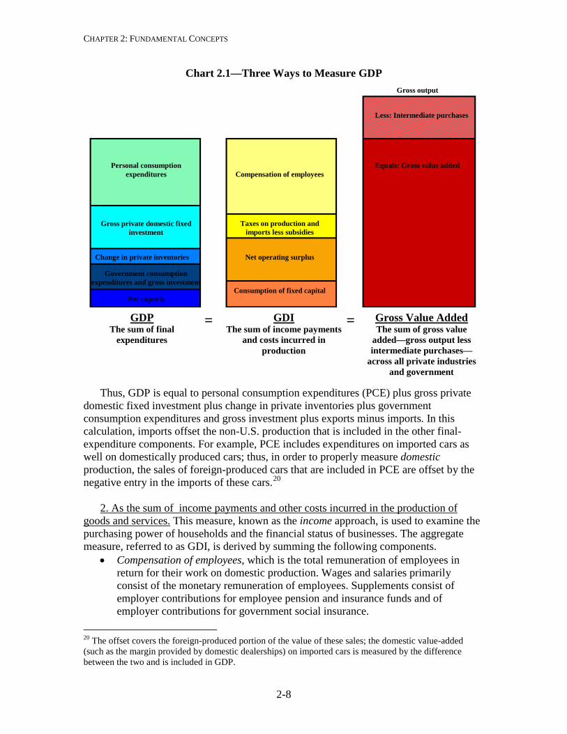
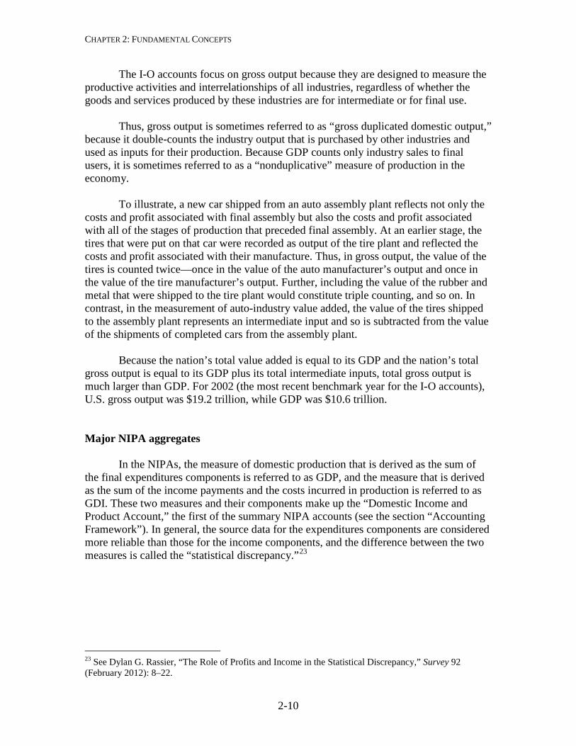
In the NIPAs, GDP is defined as the market value of the final goods and services produced by labor and property located in the United States. Conceptually, this measure can be arrived at by three separate means: as the sum of goods and services sold to final users, as the sum of income payments and other costs incurred in the production of goods and services, and as the sum of the value added at each stage of production (chart 2.1). Although these three ways of measuring GDP are conceptually the same, their calculation may not result in identical estimates of GDP because of differences in data sources, timing, and estimation techniques.

1. As the sum of goods and services sold to final users. This measure, known as the expenditures approach is used to identify the final goods and services purchased by persons, businesses, governments, and foreigners. It is arrived at by summing the following final expenditures components.

• Personal consumption expenditures, which measures the value of the goods and services purchased by persons—that is, households, nonprofit institutions that primarily serve households, private noninsured welfare funds, and private trust funds.

• Gross private fixed investment, which measures additions and replacements to the stock of private fixed assets without deduction of depreciation. Nonresidential fixed investment measures investment by businesses and nonprofit institutions in nonresidential structures and in equipment and software. Residential fixed investment measures investment by businesses and households in residential structures and equipment, primarily new construction of single-family and multifamily units.

• Change in private inventories, which measures the value of the change in the physical volume of inventories owned by private business over a specified period.

• Net exports of goods and services, which is calculated as exports less imports. Exports consist of goods and services that are sold or transferred by U.S. residents to foreign residents. Imports consist of goods and services that are sold or transferred by foreign residents to U.S. residents.

• Government consumption expenditures and gross investment, which comprises two components. Current consumption expenditures consists of the spending by general government in order to produce and provide goods and services to the public. Gross investment consists of spending by both general government and government enterprises for fixed assets that benefit the public or that assist government agencies in their productive activities.

CHAPTER 2: FUNDAMENTAL CONCEPTS

2-8

Chart 2.1—Three Ways to Measure GDP

Thus, GDP is equal to personal consumption expenditures (PCE) plus gross private

domestic fixed investment plus change in private inventories plus government consumption expenditures and gross investment plus exports minus imports. In this calculation, imports offset the non-U.S. production that is included in the other final-expenditure components. For example, PCE includes expenditures on imported cars as well on domestically produced cars; thus, in order to properly measure domestic production, the sales of foreign-produced cars that are included in PCE are offset by the negative entry in the imports of these cars.20

2. As the sum of income payments and other costs incurred in the production of

goods and services. This measure, known as the income approach, is used to examine the purchasing power of households and the financial status of businesses. The aggregate measure, referred to as GDI, is derived by summing the following components.

• Compensation of employees, which is the total remuneration of employees in return for their work on domestic production. Wages and salaries primarily consist of the monetary remuneration of employees. Supplements consist of employer contributions for employee pension and insurance funds and of employer contributions for government social insurance.

20 The offset covers the foreign-produced portion of the value of these sales; the domestic value-added (such as the margin provided by domestic dealerships) on imported cars is measured by the difference between the two and is included in GDP.

GDP The sum of final

expenditures

GDI The sum of income payments

and costs incurred in production

Gross Value Added The sum of gross value

added—gross output less intermediate purchases—

across all private industries and government

Personal consumption expenditures

Gross private domestic fixed

investment

Change in private inventories

Government consumption expenditures and gross investment

Net exports

Compensation of employees

Taxes on production and imports less subsidies

Net operating surplus

Consumption of fixed capital

Gross output

= =

Equals: Gross value added

Less: Intermediate purchases

CHAPTER 2: FUNDAMENTAL CONCEPTS

2-9

• Taxes on production and imports, which consist of taxes payable on products when they are produced, delivered, sold, transferred, or otherwise disposed of by their producers (including federal excise taxes and state and local sales taxes) and of other taxes on production, such as taxes on ownership of assets used in production (including local real estate taxes). These taxes do not include taxes on income.

• Subsidies, which are subtracted in the calculation of GDI, are monetary grants by government agencies to private business (for example, federal subsidies to farmers) and to government enterprises at another level of government (for example, federal subsidies to state and local public housing authorities).

• Net operating surplus, which is a profits-like measure that shows the incomes earned by private enterprises from current production. It is calculated by deducting the costs of compensation of employees, taxes on production and imports less subsidies, and consumption of fixed capital from value added, but before taking account of financing costs (such as net interest) and other payments (such as business current transfer payments). Net operating surplus plus consumption of fixed capital is equal to gross operating surplus.

• Consumption of fixed capital, which is the economic charge for the using up of private and government fixed capital located in the United States. It is defined as the decline in the value of the stock of assets due to wear and tear, obsolescence, accidental damage, and aging.21

Thus, GDI is equal to compensation of employees, plus taxes on production and

imports less subsidies, plus net operating surplus, plus consumption of fixed capital. Subsidies are implicitly included in the measure of net operating surplus, but because they do not represent incomes paid or costs incurred in domestic production, they must be subtracted in calculating GDI. In the NIPAs, subsidies are shown as a subtraction from “taxes on imports and production” because they are transfers from government to business and thus, in effect, represent a negative tax by government.

3. As the sum of “value added” by all industries in the economy. This measure, known as the value-added, or production, approach, is used to analyze the industrial composition of U.S. output. In the input-output (I-O) accounts, value added is defined as the difference between an industry’s gross output (sales or receipts plus other operating income and inventory change) and its intermediate inputs (goods and services that are purchased for use in production). When value added is aggregated across all industries in the economy, industry sales to and purchases from each other cancel out, and the remainder is industry sales to final users, or GDP.22

21 In the 2009 comprehensive revision, BEA introduced a new treatment of disasters in which the value of irreparable damage to, or the destruction of, fixed assets is no longer recorded as consumption of fixed capital; see Eugene P. Seskin and Shelly Smith, 11–15. 22 In the I-O accounts, “all industries” includes government industries (such as the U. S. Postal Service) and certain “special industries” (such as owner-occupied housing).

CHAPTER 2: FUNDAMENTAL CONCEPTS

2-10

The I-O accounts focus on gross output because they are designed to measure the productive activities and interrelationships of all industries, regardless of whether the goods and services produced by these industries are for intermediate or for final use.

Thus, gross output is sometimes referred to as “gross duplicated domestic output,” because it double-counts the industry output that is purchased by other industries and used as inputs for their production. Because GDP counts only industry sales to final users, it is sometimes referred to as a “nonduplicative” measure of production in the economy.

To illustrate, a new car shipped from an auto assembly plant reflects not only the

costs and profit associated with final assembly but also the costs and profit associated with all of the stages of production that preceded final assembly. At an earlier stage, the tires that were put on that car were recorded as output of the tire plant and reflected the costs and profit associated with their manufacture. Thus, in gross output, the value of the tires is counted twice—once in the value of the auto manufacturer’s output and once in the value of the tire manufacturer’s output. Further, including the value of the rubber and metal that were shipped to the tire plant would constitute triple counting, and so on. In contrast, in the measurement of auto-industry value added, the value of the tires shipped to the assembly plant represents an intermediate input and so is subtracted from the value of the shipments of completed cars from the assembly plant.

Because the nation’s total value added is equal to its GDP and the nation’s total

gross output is equal to its GDP plus its total intermediate inputs, total gross output is much larger than GDP. For 2002 (the most recent benchmark year for the I-O accounts), U.S. gross output was $19.2 trillion, while GDP was $10.6 trillion.

Major NIPA aggregates

In the NIPAs, the measure of domestic production that is derived as the sum of

the final expenditures components is referred to as GDP, and the measure that is derived as the sum of the income payments and the costs incurred in production is referred to as GDI. These two measures and their components make up the “Domestic Income and Product Account,” the first of the summary NIPA accounts (see the section “Accounting Framework”). In general, the source data for the expenditures components are considered more reliable than those for the income components, and the difference between the two measures is called the “statistical discrepancy.”23

23 See Dylan G. Rassier, “The Role of Profits and Income in the Statistical Discrepancy,” Survey 92 (February 2012): 8–22.

CHAPTER 2: FUNDAMENTAL CONCEPTS

2-11

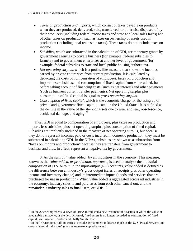
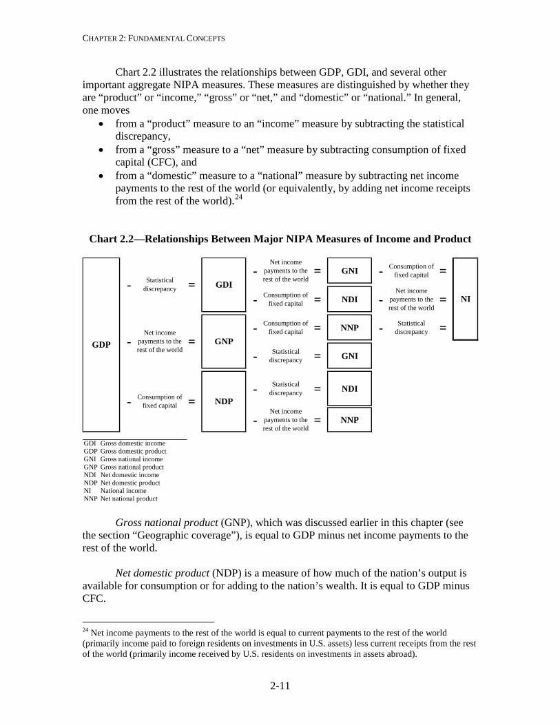
Chart 2.2 illustrates the relationships between GDP, GDI, and several other important aggregate NIPA measures. These measures are distinguished by whether they are “product” or “income,” “gross” or “net,” and “domestic” or “national.” In general, one moves

• from a “product” measure to an “income” measure by subtracting the statistical discrepancy,

• from a “gross” measure to a “net” measure by subtracting consumption of fixed capital (CFC), and

• from a “domestic” measure to a “national” measure by subtracting net income payments to the rest of the world (or equivalently, by adding net income receipts from the rest of the world).24

Chart 2.2—Relationships Between Major NIPA Measures of Income and Product

Gross national product (GNP), which was discussed earlier in this chapter (see

the section “Geographic coverage”), is equal to GDP minus net income payments to the rest of the world.

Net domestic product (NDP) is a measure of how much of the nation’s output is

available for consumption or for adding to the nation’s wealth. It is equal to GDP minus CFC.

24 Net income payments to the rest of the world is equal to current payments to the rest of the world (primarily income paid to foreign residents on investments in U.S. assets) less current receipts from the rest of the world (primarily income received by U.S. residents on investments in assets abroad).

-Net income

payments to the rest of the world

= GNI - Consumption of fixed capital =

- Consumption of fixed capital = NDI -

Net income payments to the rest of the world

=

- Consumption of fixed capital = NNP - Statistical

discrepancy =

- Statistical discrepancy = GNI

- Statistical discrepancy = NDI

-Net income

payments to the rest of the world

= NNP

GDI Gross domestic incomeGDP Gross domestic productGNI Gross national incomeGNP Gross national productNDI Net domestic incomeNDP Net domestic productNI National incomeNNP Net national product

NDP

GDINI

GNP-Net income

payments to the rest of the world

=GDP

- Consumption of fixed capital =

- Statistical discrepancy =

CHAPTER 2: FUNDAMENTAL CONCEPTS

2-12

Gross national income (GNI) measures the costs incurred and the incomes earned

in the production of GNP. It is equal to GNP minus the statistical discrepancy. It is also equal to GDI minus net income payments to the rest of the world.

Net national product (NNP) is the net market value of goods and services

produced by labor and property supplied by U.S. residents (see the earlier description of GNP). It is equal to GNP minus CFC. It is also equal to NDP minus net income payments to the rest of the world.

Net domestic income (NDI) measures the costs incurred and the incomes earned in

the production of NNP. It is equal to NNP minus the statistical discrepancy. It is also equal to GDI minus CFC.

National income is the sum of all net incomes earned in production (and thus it

could also be termed “net national income”). It is equal to GNI minus CFC, NNP minus the statistical discrepancy, and NDI minus net income payments to the rest of the world. It is also equal to the sum of compensation of employees, proprietors’ income with inventory valuation adjustment (IVA) and capital consumption adjustment (CCAdj), rental income with CCAdj, corporate profits with IVA and CCAdj, net interest and miscellaneous payments, taxes on production and imports less subsidies, business current transfer payments (net), and current surplus of government enterprises.

The following are several other important NIPA aggregates. Personal income is the income that persons receive in return for their provision of

labor, land, and capital used in current production and the net current transfer payments that they receive from business and from government.25 Personal income is equal to national income minus corporate profits with inventory valuation and capital consumption adjustments, taxes on production and imports less subsidies, contributions for government social insurance, net interest and miscellaneous payments on assets, business current transfer payments (net), current surplus of government enterprises, and wage accruals less disbursements, plus personal income receipts on assets and personal current transfer receipts.26

Gross domestic purchases is the market value of goods and services purchased by

U.S. residents, regardless of where those goods and services were produced. It is equal to GDP minus net exports. It is also equal to the sum of PCE, gross private domestic investment, and government consumption expenditures and gross investment.

Final sales of domestic product is equal to GDP less change in private

inventories. It is also equal to the sum of PCE, gross private fixed investment,

25 “Persons” consists of households, nonprofit institutions that primarily serve households, private noninsured welfare funds, and private trust funds. 26 For more information, see State Personal Income 2005 Methodology at www.bea.gov/regional/docs/spi2005.

CHAPTER 2: FUNDAMENTAL CONCEPTS

2-13

government consumption expenditures and gross investment, and net exports of goods and services.27

Final sales to domestic purchasers is equal to gross domestic purchases less

change in private inventories. It is also equal to the sum of PCE, gross private fixed investment, and government consumption expenditures and gross investment.

Principal quantity and price measures

The market values and imputations used to measure GDP and the other NIPA

estimates are in current dollars—that is, they reflect transactions in terms of their value in the periods in which they take place. Although many technical problems arise in preparing these estimates, measuring the change in current-dollar GDP from one period to the next is conceptually straightforward, because it is the actual change in spending that occurs in the economy between the two time periods.

For many analyses, it is useful to separate the changes in current-dollar GDP that

are due to changes in quantity from those that are due to changes in price.28 However, aggregate quantity change and aggregate price change cannot be observed directly in the economy. Instead, these changes must be calculated, and the calculation method is determined by analytic requirements. In the NIPAs, the changes in quantities and prices are computed from chain-type indexes that are calculated using a Fisher formula. (For a discussion of the statistical methods used to prepare these measures, see “Chapter 4: Estimating Methods.”)

In the NIPAs, the featured measure of growth in the U.S. economy is the percent

change in real GDP—that is, the quantity-change measure for GDP from one period to another.29 Thus, changes in real GDP provide a comprehensive measure of economic growth that is free of the effects of price change.

In the NIPAs, the featured measure of inflation in the U.S. economy is the percent

change in the price index for gross domestic purchases. This index measures the prices of goods and services purchased by U.S. residents, regardless of where the goods and services were produced. It is derived from the prices of PCE, gross private domestic investment, and government consumption expenditures and gross investment. Thus, for example, an increase in the import price of a foreign-produced car would raise the prices

27 While analytically useful, the interpretation of final sales of domestic product is complicated by the fact that additions to inventories come from both domestic production and imports. Source data are not available to distinguish the portion of imported goods that flows into inventories from the portion that is sold directly, so the measure does not, strictly speaking, identify the sales from domestic product. 28 In this separation, changes in the quality of the goods and services provided are treated as changes in quantity. 29 Until 1991, GNP was the featured measure of U.S. production; see “Gross Domestic Product as a Measure of U.S. Production,” Survey 71 (August 1991): 8.

CHAPTER 2: FUNDAMENTAL CONCEPTS

2-14

paid by U.S. residents and thereby directly affect the price index for gross domestic purchases.30

Another aggregate price measure is the price index for GDP, which measures the

prices of goods and services produced in the United States. In contrast to the price index for gross domestic purchases, the GDP price index would not be directly affected by an increase in the import price of a foreign-built car, because imports are not included in GDP.

Another important NIPA price measure is the PCE price index, which measures

the prices paid for the goods and services purchased by “persons.” This index is frequently compared with the consumer price index, which is produced by the Bureau of Labor Statistics. The two indexes are similar, but there are differences in terms of coverage, weighting, and calculation.31

Further, BEA provides variants of the above price indexes that exclude their

particularly volatile food and energy components. These variants are sometimes used to indicate the “core inflation” in the U.S. economy.

BEA publishes several aggregate measures of real income as counterparts to its aggregate measures of real production. Real GDI is calculated as current-dollar GDI deflated by the implicit price deflator (IPD) for GDP; real GNI is calculated as current-dollar GNI deflated by the IPD for GNP; and real net domestic income is calculated as current-dollar net domestic income deflated by the IPD for net domestic product.32

In addition, BEA prepares alternative measures of real GDP and real GNP that

measure the real purchasing power of the income generated from the production of the goods and services by the U.S. economy. These measures, which in the NIPAs are called command-basis GDP and command-basis GNP, reflect the impact of changes in the terms of trade as well as changes in production (BEA also prepares alternative command-basis measures of NNP and NDP).33 In calculating command-basis GDP, exports and imports of goods and services are each deflated by the price index for gross domestic purchases to yield exports on a command-basis and imports on a command basis; then, command-basis exports are added to, and command-basis imports are subtracted from, real gross domestic purchases.34 The calculation of command-basis GNP is the same, except income receipts from the rest of the world are deflated along with exports, and

30 This example assumes the entire price increase is passed on to the car buyer—that is, the wholesale or retail margins are unchanged. 31 See Clinton P. McCully, Brian C. Moyer, and Kenneth J. Stewart, “Comparing the Consumer Price Index and the Personal Consumption Expenditures Price Index,” Survey 87 (November 2007): 26–33. 32 Implicit price deflators for an aggregate or component are calculated as the ratio of the current-dollar value to the corresponding chained-dollar value, multiplied by 100 (see the section “Chained-dollar measures” in chapter 4). 33 In the SNAs, these measures are referred to as real GDI and real GNI. However, as noted in the preceding paragraph, BEA uses a different method to derive those aggregates. 34 In this case, adding and subtracting these estimates is acceptable because all three aggregates are derived using the same deflator.

CHAPTER 2: FUNDAMENTAL CONCEPTS

2-15

income payments to the rest of the world are deflated along with imports.35 In effect, the calculations are the same as deriving command-basis GDP (GNP) by deflating current-dollar GDP (GNP) by the price index for gross domestic purchases. Thus, the command-basis measures are alternative measures of real GDP and real GNP that reflect the prices of purchased goods and services, while the primary measures of real GDP and real GNP reflect the prices of produced goods and services.

BEA also prepares several measures that show the relationship between the prices that are received by U.S. producers and the prices that are paid by U.S. purchasers. The broadest measure, the trading gains index, is the ratio of the GDP price index to the price index for gross domestic purchases. An increase (decrease) in this ratio would indicate an increase (decrease) in the purchasing power of the income generated in producing GDP. Successively narrower measures specifically focus on the relationship between the prices of the U.S. goods and services that are produced for consumption by the rest of the world and the prices of the goods and services that are produced by the rest of the world for U.S. consumption. The terms of trade index, is the ratio of the price index for exports of goods and services to the price index for imports of goods and services; ratios for the terms of trade in goods and in nonpetroleum goods are also prepared. Movements in these trading indexes reflect the interaction of several factors—including movements in exchange rates, changes in the composition of traded goods and services, and changes in producers’ profit margins.

In addition, BEA provides statistical measures that supplement the current-dollar,

quantity-index, and price-index measures. Foremost among these are measures of the contributions of major components to the percent change from the preceding year or quarter in real GDP, in other principal product-side aggregates, in GDP prices, and in gross domestic purchases prices. BEA also provides measures of the percentage shares of current-dollar GDP and GDI that are accounted for by their major components.

Classification

The application of common classification systems for the NIPAs, and for all of the U.S. economic accounts, is extremely important because classification provides the structure necessary to prepare and present the estimates uniformly and consistently. Further, common classifications enable users to effectively compare and analyze data across the broad spectrum of economic statistics.

35 This methodology for calculating the command-basis aggregates was introduced in the 2010 annual revision of the NIPAs; see Eugene P. Seskin and Shelly Smith, “Annual Revision of the National Income and Product Accounts,” Survey 90 (August 2010): 21. For additional technical and historical background, see Marshall B. Reinsdorf, “Terms of Trade Effects: Theory and Measurement,” Review of Income and Wealth 56 (June 2010): S177-S205.

CHAPTER 2: FUNDAMENTAL CONCEPTS

2-16

In the NIPAs, the estimates of production and expenditures may be classified by sector, by type of product, and by function, while the estimates of income may be classified by industry and by legal form of organization. Sector

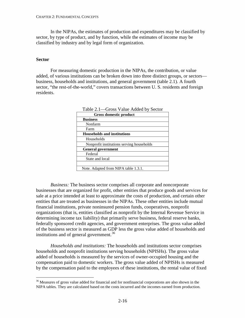
For measuring domestic production in the NIPAs, the contribution, or value added, of various institutions can be broken down into three distinct groups, or sectors—business, households and institutions, and general government (table 2.1). A fourth sector, “the rest-of-the-world,” covers transactions between U. S. residents and foreign residents.

Table 2.1—Gross Value Added by Sector Gross domestic product Business Nonfarm Farm Households and institutions Households Nonprofit institutions serving households General government Federal State and local Note. Adapted from NIPA table 1.3.1.

Business: The business sector comprises all corporate and noncorporate businesses that are organized for profit, other entities that produce goods and services for sale at a price intended at least to approximate the costs of production, and certain other entities that are treated as businesses in the NIPAs. These other entities include mutual financial institutions, private noninsured pension funds, cooperatives, nonprofit organizations (that is, entities classified as nonprofit by the Internal Revenue Service in determining income tax liability) that primarily serve business, federal reserve banks, federally sponsored credit agencies, and government enterprises. The gross value added of the business sector is measured as GDP less the gross value added of households and institutions and of general government.36

Households and institutions: The households and institutions sector comprises

households and nonprofit institutions serving households (NPISHs). The gross value added of households is measured by the services of owner-occupied housing and the compensation paid to domestic workers. The gross value added of NPISHs is measured by the compensation paid to the employees of these institutions, the rental value of fixed

36 Measures of gross value added for financial and for nonfinancial corporations are also shown in the NIPA tables. They are calculated based on the costs incurred and the incomes earned from production.

CHAPTER 2: FUNDAMENTAL CONCEPTS

2-17

assets owned and used by these institutions, and the rental income of persons for tenant-occupied housing owned by these institutions.37

General government: The general government sector comprises all federal

government and state and local government agencies except government enterprises. The gross value added of general government is measured as the sum of the compensation of the employees of these agencies and of their consumption of fixed capital.

Type of product

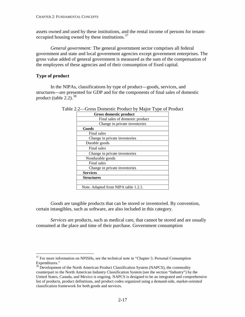
In the NIPAs, classifications by type of product—goods, services, and structures—are presented for GDP and for the components of final sales of domestic product (table 2.2).38

Table 2.2—Gross Domestic Product by Major Type of Product

Gross domestic product Final sales of domestic product Change in private inventories Goods Final sales Change in private inventories Durable goods Final sales Change in private inventories Nondurable goods Final sales Change in private inventories Services Structures Note. Adapted from NIPA table 1.2.1.

Goods are tangible products that can be stored or inventoried. By convention, certain intangibles, such as software, are also included in this category.

Services are products, such as medical care, that cannot be stored and are usually

consumed at the place and time of their purchase. Government consumption

37 For more information on NPISHs, see the technical note in “Chapter 5: Personal Consumption Expenditures.” 38 Development of the North American Product Classification System (NAPCS), the commodity counterpart to the North American Industry Classification System (see the section “Industry”) by the United States, Canada, and Mexico is ongoing. NAPCS is designed to be an integrated and comprehensive list of products, product definitions, and product codes organized using a demand-side, market-oriented classification framework for both goods and services.

CHAPTER 2: FUNDAMENTAL CONCEPTS

2-18

expenditures, which are for services produced by government, are included in this category.39 By convention, goods purchased by U.S. residents abroad are also included.

Structures are products—such as commercial buildings, highways, dams, and

single-family houses—that are usually constructed at the location where they will be used and that typically have long economic lives.

Function “Functional” classifications identify the purposes or objectives for which

expenditures are made. In the NIPAs, functional breakdowns of expenditures are provided for PCE and for government expenditures.

For PCE, a new classification system was introduced in the 2009 comprehensive

revision (see “Chapter 5: Personal Consumption Expenditures”).40 In the new structure, expenditures by function are classified into the following broad categories (table 2.3). These classifications are largely consistent with the SNA “Classification of Individual Consumption by Purpose” (COICOP).41

Table 2.3—Personal Consumption Expenditures by Function Personal consumption expenditures Food and beverages purchased for off-premises consumption Clothing, footwear, and related services Housing, utilities, and fuels Furnishings, household equipment, and routine household maintenance Health Transportation Communication Recreation Education Food services and accommodations Financial services and insurance Other goods and services Net foreign travel and expenditures abroad by U.S. residents Final consumption expenditures of nonprofit institutions serving households Note. Adapted from NIPA table 2.5.5.

39 The value of these services, most of which are not sold in the market, is measured by the cost of inputs: compensation, CFC, and purchased goods and services less own-account investment and sales to other sectors (which are reflected in other final expenditures components, such as PCE). 40 See also Clinton P. McCully and Teresita D. Teensma, “Preview of the 2009 Comprehensive Revision of the National Income and Product Accounts: New Classifications for Personal Consumption Expenditures,” Survey 88 (May 2008): 6–17. 41 McCully and Teensma, 14.

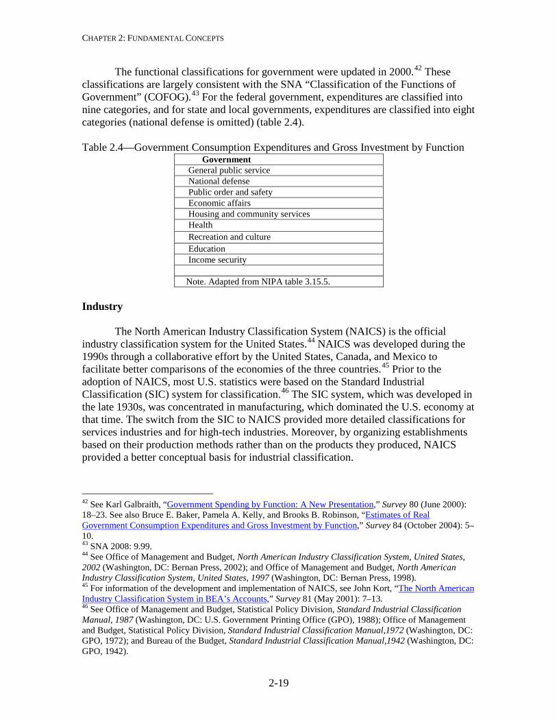
CHAPTER 2: FUNDAMENTAL CONCEPTS

2-19

The functional classifications for government were updated in 2000.42 These classifications are largely consistent with the SNA “Classification of the Functions of Government” (COFOG).43 For the federal government, expenditures are classified into nine categories, and for state and local governments, expenditures are classified into eight categories (national defense is omitted) (table 2.4).

Table 2.4—Government Consumption Expenditures and Gross Investment by Function

Government General public service National defense Public order and safety Economic affairs Housing and community services Health Recreation and culture Education Income security Note. Adapted from NIPA table 3.15.5.

Industry

The North American Industry Classification System (NAICS) is the official

industry classification system for the United States.44 NAICS was developed during the 1990s through a collaborative effort by the United States, Canada, and Mexico to facilitate better comparisons of the economies of the three countries.45 Prior to the adoption of NAICS, most U.S. statistics were based on the Standard Industrial Classification (SIC) system for classification.46 The SIC system, which was developed in the late 1930s, was concentrated in manufacturing, which dominated the U.S. economy at that time. The switch from the SIC to NAICS provided more detailed classifications for services industries and for high-tech industries. Moreover, by organizing establishments based on their production methods rather than on the products they produced, NAICS provided a better conceptual basis for industrial classification.

42 See Karl Galbraith, “Government Spending by Function: A New Presentation,” Survey 80 (June 2000): 18–23. See also Bruce E. Baker, Pamela A. Kelly, and Brooks B. Robinson, “Estimates of Real Government Consumption Expenditures and Gross Investment by Function,” Survey 84 (October 2004): 5–10. 43 SNA 2008: 9.99. 44 See Office of Management and Budget, North American Industry Classification System, United States, 2002 (Washington, DC: Bernan Press, 2002); and Office of Management and Budget, North American Industry Classification System, United States, 1997 (Washington, DC: Bernan Press, 1998). 45 For information of the development and implementation of NAICS, see John Kort, “The North American Industry Classification System in BEA’s Accounts,” Survey 81 (May 2001): 7–13. 46 See Office of Management and Budget, Statistical Policy Division, Standard Industrial Classification Manual, 1987 (Washington, DC: U.S. Government Printing Office (GPO), 1988); Office of Management and Budget, Statistical Policy Division, Standard Industrial Classification Manual,1972 (Washington, DC: GPO, 1972); and Bureau of the Budget, Standard Industrial Classification Manual,1942 (Washington, DC: GPO, 1942).

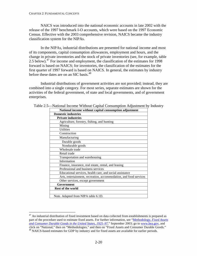
CHAPTER 2: FUNDAMENTAL CONCEPTS

2-20

NAICS was introduced into the national economic accounts in late 2002 with the release of the 1997 benchmark I-O accounts, which were based on the 1997 Economic Census. Effective with the 2003 comprehensive revision, NAICS became the industry classification system for the NIPAs.

In the NIPAs, industrial distributions are presented for national income and most of its components, capital consumption allowances, employment and hours, and the change in private inventories and the stock of private inventories (see, for example, table 2.5 below).47 For income and employment, the classification of the estimates for 1998 forward is based on NAICS; for inventories, the classification of the estimates for the first quarter of 1997 forward is based on NAICS. In general, the estimates by industry before these dates are on an SIC basis.48

Industrial distributions of government activities are not provided; instead, they are

combined into a single category. For most series, separate estimates are shown for the activities of the federal government, of state and local governments, and of government enterprises.

Table 2.5—National Income Without Capital Consumption Adjustment by Industry

National income without capital consumption adjustment Domestic industries Private industries Agriculture, forestry, fishing, and hunting Mining Utilities Construction Manufacturing Durable goods Nondurable goods Wholesale trade Retail trade Transportation and warehousing Information Finance, insurance, real estate, rental, and leasing Professional and business services Educational services, health care, and social assistance Arts, entertainment, recreation, accommodation, and food services Other services, except government Government Rest of the world Note. Adapted from NIPA table 6.1D.

47 An industrial distribution of fixed investment based on data collected from establishments is prepared as part of the procedure used to estimate fixed assets. For further information, see “Methodology, Fixed Assets and Consumer Durable Goods in the United States, 1925–97,” September 2003; go to www.bea.gov, and click on “National,” then on “Methodologies,” and then on “Fixed Assets and Consumer Durable Goods.” 48 NAICS-based estimates for GDP by industry and for fixed assets are available for earlier periods.

CHAPTER 2: FUNDAMENTAL CONCEPTS

2-21

The industrial distributions for wages and salaries and for inventories are generally based on data collected from “establishments,” while those for the other NIPA components are generally based on data collected from “companies” (also called “enterprises,” or “firms”). Companies consist of one or more establishments owned by the same legal entity or group of affiliated entities. Establishments are economic units, generally at a single physical location, where business is conducted or where services or industrial operations are performed (for example a factory, mill, store, hotel, movie theater, mine, farm, airline terminal, sales office, warehouse, or central administrative office). Establishments are classified into an industry on the basis of their principal production method, and companies are classified into an industry on the basis of the principal industry of all their establishments. Because large multi-establishment companies typically contain establishments that are classified in different industries, the industrial distribution of the same economic activity on an establishment basis can differ significantly from that on a company basis. For example, the measure of employment by steel-manufacturing companies will include the employment of establishments that do not manufacture steel but are part of companies that are classified as steel-manufacturing companies. Similarly, this measure will exclude the employment of establishments that manufacture steel but are part of companies that are not classified as steel-manufacturing companies.

Moreover, individual industry series are not fully comparable over time. First, the

composition of industries may change because of revisions to NAICS or to the SIC. This factor affects estimates based on establishment data and on company data. Second, historical comparability may be affected by a change over time in the industrial classification of the same establishment or company. For example, the classification of a company may change as a result of shifts in the level of consolidation of entities for which company reports are filed or as a result of mergers and acquisitions. This factor affects company-based estimates much more than establishment-based estimates.

In addition, some NIPA tables show the following special industry groupings: Financial industries consists of the NAICS industry “Finance and insurance” and

of “Offices of bank holding companies” and “Offices of other holding companies” in the NAICS industry “Management of companies and enterprises.” Finance and insurance consists of Federal Reserve banks; credit intermediation and related activities; securities, commodity contracts, and investments; insurance carriers and related activities; and funds, trusts, and other financial vehicles.

Nonfinancial industries consists of all other private industries. Private goods-producing industries consists of the following NAICS divisions:

agriculture, forestry, fishing, and hunting; mining; construction; and manufacturing. Private services-producing industries consists of the following NAICS divisions:

utilities; wholesale trade; retail trade; transportation and warehousing; information; finance and insurance; real estate and rental and leasing; professional, scientific, and

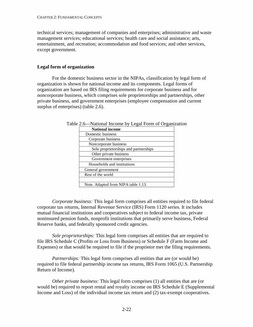
CHAPTER 2: FUNDAMENTAL CONCEPTS

2-22

technical services; management of companies and enterprises; administrative and waste management services; educational services; health care and social assistance; arts, entertainment, and recreation; accommodation and food services; and other services, except government. Legal form of organization

For the domestic business sector in the NIPAs, classification by legal form of organization is shown for national income and its components. Legal forms of organization are based on IRS filing requirements for corporate business and for noncorporate business, which comprises sole proprietorships and partnerships, other private business, and government enterprises (employee compensation and current surplus of enterprises) (table 2.6).

Table 2.6—National Income by Legal Form of Organization National income Domestic business Corporate business Noncorporate business Sole proprietorships and partnerships Other private business Government enterprises Households and institutions General government Rest of the world Note. Adapted from NIPA table 1.13.

Corporate business: This legal form comprises all entities required to file federal

corporate tax returns, Internal Revenue Service (IRS) Form 1120 series. It includes mutual financial institutions and cooperatives subject to federal income tax, private noninsured pension funds, nonprofit institutions that primarily serve business, Federal Reserve banks, and federally sponsored credit agencies.

Sole proprietorships: This legal form comprises all entities that are required to

file IRS Schedule C (Profits or Loss from Business) or Schedule F (Farm Income and Expenses) or that would be required to file if the proprietor met the filing requirements.

Partnerships: This legal form comprises all entities that are (or would be)

required to file federal partnership income tax returns, IRS Form 1065 (U.S. Partnership Return of Income).

Other private business: This legal form comprises (1) all entities that are (or

would be) required to report rental and royalty income on IRS Schedule E (Supplemental Income and Loss) of the individual income tax return and (2) tax-exempt cooperatives.

CHAPTER 2: FUNDAMENTAL CONCEPTS

2-23

Government enterprises: This legal form consists of government agencies that

cover a substantial proportion of their operating costs by selling goods and services to the public and that maintain their own separate accounts. For example, the U.S. Postal Service is a federal government enterprise, and public water and sewage agencies are local government enterprises.

Accounting Framework

The NIPAs consist of a set of integrated accounts that provide statistics on the output of the U.S. economy. The NIPA accounting framework is designed to provide context for these statistics, so that they are presented logically, consistently, and according to established economic-accounting principles and standards. The NIPAs are generally consistent with the SNA, which now serves as the internationally accepted set of guidelines for the compilation of national accounts.49

For an in-depth discussion of the conceptual framework of the NIPAs and the NIPA summary accounts and of the underlying accounting principles and common financial statements, see U.S. Bureau of Economic Analysis, An Introduction to National Economic Accounting, Methodology Paper No. 1 (updated), September 2007.50

Accounting principles Double-entry bookkeeping is one of the most fundamental principles used in economic accounting and in financial accounting. In financial accounting, activities that affect the resources available to a business are recorded at least once as a source of financing (credit) and at least once as a use of financing (debit). Thus, double-entry bookkeeping provides a means to validate the accounting entries, because the sum of the entries on each side of an account must be equal. In national economic accounting, each transaction is recorded as a payment by one sector and as a receipt by the same sector or by another sector—for example corporate income tax is a payment by a corporation and a receipt of the government.51 In addition to providing a means to validate entries, this system also provides alternative ways to calculate a measure when complete information is not available for one of the sectors.

The accrual-accounting method is another principle important to both financial

and economic accounting. This method is generally used to ensure that related revenues 49 See Charles Ian Mead, Karin E. Moses, and Brent R. Moulton, “The NIPAs and the System of National Accounts,” Survey 84 (December 2004): 17–32. 50 Go to www.bea.gov, and click on “National,” then on “Methodologies.” 51 A fully articulated set of national accounts (showing payments and receipts by all sectors) actually leads to a quadruple-entry system (in which each transaction is recorded as a debit and a change in assets for one sector and as a credit and a change in assets for another sector) . However, transactions are usually recorded only twice in the NIPAs because the changes in assets or liabilities that are associated with the changes in revenues or expenses are recorded in the Federal Reserve Board’s flow of funds accounts.

CHAPTER 2: FUNDAMENTAL CONCEPTS

2-24

and expenses are recorded in the same accounting period. In accrual accounting, revenues are recorded when they are earned, and expenses are recorded when they are incurred, regardless of when the cash is actually received or paid. The accrual-accounting method may be contrasted to the cash-accounting method, which records revenues when cash is received and expenses when cash is paid.

Financial accounting and economic accounting generally apply different

principles in valuing transactions. In financial accounting, assets (and depreciation) are commonly valued at historical costs—that is, at the prices relevant at the time of the acquisition; subsequent changes in the value of these assets are ignored. In economic accounting, assets (and depreciation) are valued at current costs—that is, at the market prices that prevail at the time they are valued. In preparing the NIPAs, various adjustments, such as the inventory valuation adjustment and the capital consumption adjustment, are made so that the estimates will reflect current costs rather than historical costs.

Conceptual derivation of the NIPAs The NIPAs represent consolidations of the production, the income and outlay, and the saving and investment accounts for each sector of the economy (business, households, government, and foreign). These sector accounts, in turn, represent aggregations of the accounts belonging to individual transactors in the economy, regardless of whether formal accounting statements exist explicitly for all of them. Specifically, for each sector, the production account records the value of the production that is attributable to that sector and the uses of the income arising from that production. The income and outlay account records the sources of the sector’s income, its current outlays, and its saving. The saving and investment account (also known as the capital account) records the sector’s gross saving and gross investment, where gross investment is net acquisitions of assets less net increase in liabilities. Chart 2.3 illustrates the relationship between the summary NIPAs and the underlying production, income and outlay, and saving and investment accounts for the sectors of the economy.

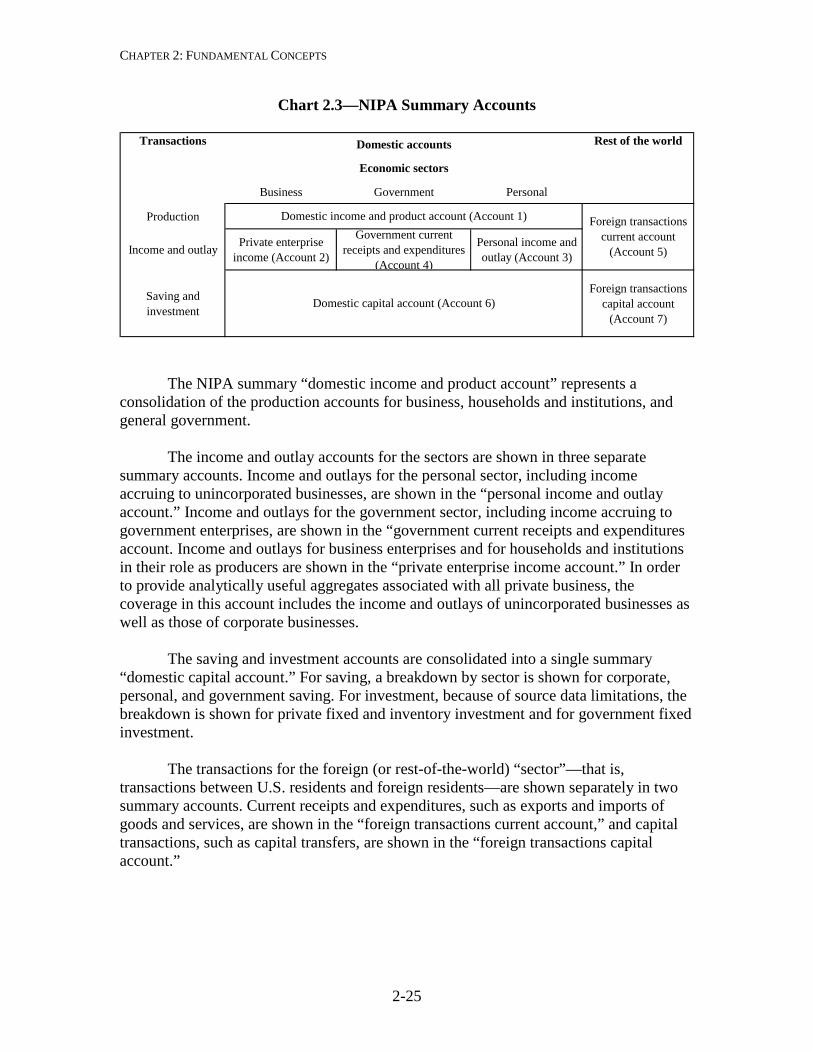
CHAPTER 2: FUNDAMENTAL CONCEPTS

2-25

Chart 2.3—NIPA Summary Accounts

The NIPA summary “domestic income and product account” represents a consolidation of the production accounts for business, households and institutions, and general government. The income and outlay accounts for the sectors are shown in three separate summary accounts. Income and outlays for the personal sector, including income accruing to unincorporated businesses, are shown in the “personal income and outlay account.” Income and outlays for the government sector, including income accruing to government enterprises, are shown in the “government current receipts and expenditures account. Income and outlays for business enterprises and for households and institutions in their role as producers are shown in the “private enterprise income account.” In order to provide analytically useful aggregates associated with all private business, the coverage in this account includes the income and outlays of unincorporated businesses as well as those of corporate businesses. The saving and investment accounts are consolidated into a single summary “domestic capital account.” For saving, a breakdown by sector is shown for corporate, personal, and government saving. For investment, because of source data limitations, the breakdown is shown for private fixed and inventory investment and for government fixed investment. The transactions for the foreign (or rest-of-the-world) “sector”—that is, transactions between U.S. residents and foreign residents—are shown separately in two summary accounts. Current receipts and expenditures, such as exports and imports of goods and services, are shown in the “foreign transactions current account,” and capital transactions, such as capital transfers, are shown in the “foreign transactions capital account.”

Business Government Personal

Production

Income and outlay Private enterprise income (Account 2)

Government current receipts and expenditures

(Account 4)

Personal income and outlay (Account 3)

Saving and investment

Foreign transactions capital account

(Account 7)Domestic capital account (Account 6)

Domestic accounts

Economic sectors

Foreign transactions current account

(Account 5)

Rest of the worldTransactions

Domestic income and product account (Account 1)

CHAPTER 2: FUNDAMENTAL CONCEPTS

2-26

The summary NIPAs The seven summary NIPAs constitute the accounting framework for presenting the value of production, distribution, consumption, and saving for the U.S. economy.52 (For a full presentation of the summary accounts, see table 2.A at the end of this chapter.) Each of the entries in a summary account also appears again in that account or in one of the other summary accounts; most of these entries are also shown in one or more of the tables that make up the full set of NIPA tables. For example, the item “supplements to wages and salaries” is shown in line 5 of summary account 1 and in line 14 of summary account 3; it is also shown in line 8 of NIPA table 1.10 and in line 6 of NIPA table 2.1.

Taken together, the summary accounts constitute a double-entry system in which a use (or expenditure) recorded in one account for one sector is also recorded as a source (or receipt) in an account of another sector or of the same sector. This system of integrated, double-entry accounts provides a comprehensive measure of economic activity in a consistently defined framework without double-counting. Thus, the NIPAs, in combination with BEA’s industry, wealth, and other economic accounts, can be used to trace the principal economic flows among the major sectors of the economy. Account 1: Domestic Income and Product Account

This account represents an aggregation of the underlying production accounts for the domestic sectors of the U.S. economy. The right (product) side of the account shows GDP measured as the sum of goods and services sold to final users rather than as the sum of value-added by the sectors. The left (income) side of the account shows GDP as measured by the incomes earned in production—GDI—plus the “statistical discrepancy” (the difference between GDP and GDI). Product and income are both presented on a domestic basis—that is, they are produced by labor and property located in the United States. Account 2: Private Enterprise Income Account

This account presents information on the sources and uses of the income of private businesses and other private enterprises.53 It combines the accounts of private businesses, of homeowners for owner-occupied housing (which is treated as if it were a business), and of NPISHs.

52 Prior to the 2003 comprehensive revision, the NIPAs were summarized in five accounts, as shown in table A on pages 38–39 of the August 2002 Survey. For a discussion of the differences between the old and new summary accounts, see Nicole Mayerhauser, Shelly Smith, and David F. Sullivan, “Preview of the 2003 Comprehensive Revision of the National Income and Product Accounts: New and Redesigned Tables,” Survey 83 (August 2003): 8–15. 53 Government enterprises are not included in account 2, because complete estimates on sources and uses of government enterprise income, notably the income payments and income receipts on assets, are not currently available. The sources and uses of government enterprise income are included, but not separately identified, in the government receipts and expenditures account.

CHAPTER 2: FUNDAMENTAL CONCEPTS

2-27

Sources of private enterprise income—such as interest receipts on assets and net operating surplus—are shown on the right side of the account.54 The left side of the account shows the uses of income as income payments on assets (such as holders of financial liabilities and equity claims of other businesses), business current transfer payments, and income that accrues to the owners of business (namely proprietors’ income, rental income of persons, and corporate profits. Corporate profits, a widely used measure in the United States, is distributed to government (taxes on corporate income) and to shareholders (net dividends) or is retained (undistributed profits, which can be thought of as a measure of corporate saving). Account 3: Personal Income and Outlay Account

This account shows the sources and uses of income received by persons—that is, households, NPISHs, private noninsured welfare funds, and private trust funds. The right side of the account shows the sources of personal income—such as employee compensation and interest and dividend income. The left side shows personal taxes and outlays and personal saving, which is derived as personal income minus personal taxes and outlays. Account 4: Government Receipts and Expenditures Account

This account summarizes the combined transactions of the federal government and of the state and local governments. The right side of the account shows government current receipts—such as tax receipts from persons and contributions for government social insurance. The left side shows government current expenditures—such as compensation of government employees and transfer payments to persons—and net saving, which is derived as current receipts less current expenditures. Account 5: Foreign Transactions Current Account

This account summarizes all the current transactions between the United States and the rest of the world. It presents information on receipts and payments associated with foreign trade and other transactions not involving transfers of assets. The left side of the account shows current receipts from the rest of the world—mainly exports of goods and services and income receipts on assets. The right side shows current payments to the rest of the world—mainly imports of goods and services, income payments on assets, and current taxes and transfer payments. In addition, it includes the balance on current account, which is derived as current receipts less current payments.

54 Summary account 2 presents the components of private enterprise income on a national basis—that is, for income accruing to U.S. residents. Consequently, for the net operating surplus to be shown in account 2 on a domestic basis consistent with summary account 1, several components showing income flows to and from the rest of the world are added to account 2.

CHAPTER 2: FUNDAMENTAL CONCEPTS

2-28

Account 6: Domestic Capital Account

This account presents information on saving and investment for the economy. The right side of the account shows gross saving and the statistical discrepancy. Given the theoretical equality between GDP and GDI, the statistical discrepancy can be viewed as actual (positive or negative) income that is not captured by the data used to measure GDI and, therefore, not distributed to the sectors; instead, it is shown as a source of (positive or negative) saving in this account. The left side of the account shows gross domestic investment, capital-account transactions (net), and net lending or net borrowing, which is derived as gross saving and the statistical discrepancy minus gross domestic investment and capital-account transactions (net). Account 7: Foreign Transactions Capital Account

This account presents information on transactions between the United States and the rest of the world that are linked to the acquisition or disposition of nonproduced nonfinancial assets and capital transfers. The left side of the account shows the balance on current account. The right side shows capital-account transactions (net) and net lending or borrowing, which is derived as the balance on current account minus capital-account transactions (net).

CHAPTER 2: FUNDAMENTAL CONCEPTS

Table A. Summary National Income and Product Accounts, 2011 [Billions of dollars]

Account 1. Domestic Income and Product Account

Line Line

1 Compensation of employees, paid ......................................................................... 8,303.2 15 Personal consumption expenditures (3–3) ............................................................ 10,729.0 2 Wage and salary accruals.................................................................................. 6,669.3 16 Goods ................................................................................................................ 3,624.8 3 Disbursements (3–12 plus 5–11) ................................................................... 6,669.3 17 Durable goods ............................................................................................... 1,146.4 4 Wage accruals less disbursements (4–9 plus 6–13)...................................... 0.0 18 Nondurable goods ......................................................................................... 2,478.4 5 Supplements to wages and salaries (3–14) ....................................................... 1,633.9 19 Services............................................................................................................. 7,104.2 6 Taxes on production and imports (4–16)................................................................ 1,097.9 20 Gross private domestic investment........................................................................ 1,854.9 7 Less: Subsidies (4–8)............................................................................................. 61.6 21 Fixed investment (6–2) ...................................................................................... 1,818.3 8 Net operating surplus............................................................................................. 3,767.6 22 Nonresidential................................................................................................ 1,479.6 9 Private enterprises (2–19).................................................................................. 3,794.1 23 Structures .................................................................................................. 404.8

10 Current surplus of government enterprises (4–26) ............................................ –26.5 24 Equipment and software............................................................................ 1,074.7 11 Consumption of fixed capital (6–15)....................................................................... 1,936.8 25 Residential..................................................................................................... 338.7

26 Change in private inventories (6–4)................................................................... 36.6 12 Gross domestic income ...................................................................................... 15,043.8 27 Net exports of goods and services ........................................................................ –568.1

28 Exports (5–1) ..................................................................................................... 2,094.2 13 Statistical discrepancy (6–21) ................................................................................ 31.9 29 Imports (5–9) ..................................................................................................... 2,662.3

30 Government consumption expenditures and gross investment (4–1 plus 6–3) ..... 3,059.8 31 Federal............................................................................................................... 1,222.1 32 National defense............................................................................................ 820.8 33 Nondefense ................................................................................................... 401.3 34 State and local................................................................................................... 1,837.7

14 GROSS DOMESTIC PRODUCT............................................................................ 15,075.7 35 GROSS DOMESTIC PRODUCT ........................................................................... 15,075.7

Account 2. Private Enterprise Income Account

Line Line

1 Income payments on assets................................................................................... 2,352.4 19 Net operating surplus, private enterprises (1–9) ................................................... 3,794.1 2 Interest and miscellaneous payments (3–20 and 4–21) .................................... 2,146.1 20 Income receipts on assets ..................................................................................... 2,084.9 3 Dividend payments to the rest of the world (5–14)............................................. 118.8 21 Interest (3–20) ................................................................................................... 1,439.7 4 Reinvested earnings on foreign direct investment in the United States (5–15) 87.5 22 Dividend receipts from the rest of the world (5–6)............................................. 262.0 5 Business current transfer payments (net) .............................................................. 132.6 23 Reinvested earnings on U.S. direct investment abroad (5–7)............................ 383.2 6 To persons (net) (3–24)...................................................................................... 44.9 7 To government (net) (4–24)................................................................................ 94.8 8 To the rest of the world (net) (5–19) ................................................................... –7.1 9 Proprietors’ income with inventory valuation and capital consumption

adjustments (3–17) ............................................................................................ 1,157.3 10 Rental income of persons with capital consumption adjustment (3–18) ................ 409.7 11 Corporate profits with inventory valuation and capital consumption adjustments 1,827.0 12 Taxes on corporate income ................................................................................ 379.0 13 To government (4–17) .................................................................................... 351.8 14 To the rest of the world (5–19) ....................................................................... 27.2 15 Profits after tax with inventory valuation and capital consumption adjustments 1,447.9 16 Net dividends (3–21 plus 4–22) ..................................................................... 697.2 17 Undistributed corporate profits with inventory valuation and capital

consumption adjustments (6–12)............................................................... 750.7

18 USES OF PRIVATE ENTERPRISE INCOME ........................................................ 5,879.0 24 SOURCES OF PRIVATE ENTERPRISE INCOME................................................ 5,879.0

Account 3. Personal Income and Outlay Account

Line Line

1 Personal current taxes (4–15) ................................................................................ 1,398.0 10 Compensation of employees, received .................................................................. 8,295.2 2 Personal outlays..................................................................................................... 11,059.9 11 Wage and salary disbursements ....................................................................... 6,661.3 3 Personal consumption expenditures (1–15)....................................................... 10,729.0 12 Domestic (1–3 less 5–11).............................................................................. 6,655.5 4 Personal interest payments (3–20) .................................................................... 168.0 13 Rest of the world (5–3) .................................................................................. 5.8 5 Personal current transfer payments ................................................................... 162.8 14 Supplements to wages and salaries (1–5) ........................................................ 1,633.9 6 To government (4–25) .................................................................................... 88.9 15 Employer contributions for employee pension and insurance funds.............. 1,139.0 7 To the rest of the world (net) (5–17) ............................................................... 73.9 16 Employer contributions for government social insurance............................... 494.9

17 Proprietors’ income with inventory valuation and capital consumption 8 Personal saving (6–11) .......................................................................................... 489.4 adjustments (2–9).............................................................................................. 1,157.3

18 Rental income of persons with capital consumption adjustment (2–10)................ 409.7 19 Personal income receipts on assets ...................................................................... 1,685.1 20 Personal interest income (2–2 plus 3–4 plus 4–7 plus 5–5 less 2–21 less 4–21

less 5–13) ...................................................................................................... 1,008.8 21 Personal dividend income (2–16 less 4–22) ...................................................... 676.3 22 Personal current transfer receipts .......................................................................... 2,319.2 23 Government social benefits (4–4)...................................................................... 2,274.3 24 From business (net) (2–6).................................................................................. 44.9 25 Less: Contributions for government social insurance, domestic (4–19) ................ 919.3

9 PERSONAL TAXES, OUTLAYS, AND SAVING.................................................... 12,947.3 26 PERSONAL INCOME ........................................................................................... 12,947.3

2–29

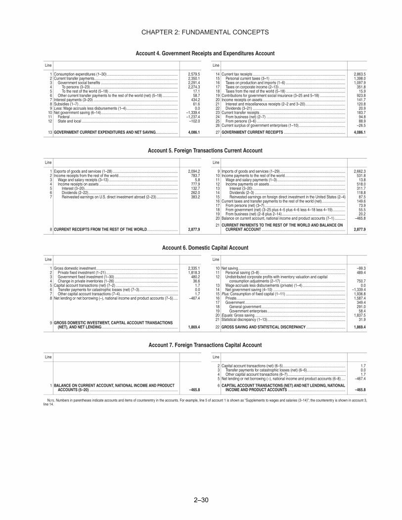
Account 4. Government Receipts and Expenditures Account

Line Line

1 Consumption expenditures (1–30) ......................................................................... 2,579.5 14 Current tax receipts ............................................................................................... 2,863.5 2 Current transfer payments...................................................................................... 2,350.1 15 Personal current taxes (3–1) ............................................................................. 1,398.0 3 Government social benefits ............................................................................... 2,291.4 16 Taxes on production and imports (1–6) ............................................................. 1,097.9 4 To persons (3–23) .......................................................................................... 2,274.3 17 Taxes on corporate income (2–13) .................................................................... 351.8 5 To the rest of the world (5–18) ....................................................................... 17.1 18 Taxes from the rest of the world (5–18) ............................................................. 15.9 6 Other current transfer payments to the rest of the world (net) (5–18) ................ 58.7 19 Contributions for government social insurance (3–25 and 5–18) .......................... 923.8 7 Interest payments (3–20) ....................................................................................... 434.2 20 Income receipts on assets..................................................................................... 141.7 8 Subsidies (1–7) ...................................................................................................... 61.6 21 Interest and miscellaneous receipts (2–2 and 3–20)......................................... 120.8 9 Less: Wage accruals less disbursements (1–4)..................................................... 0.0 22 Dividends (3–21) ............................................................................................... 20.9

10 Net government saving (6–14)............................................................................... –1,339.4 23 Current transfer receipts ........................................................................................ 183.7 11 Federal ............................................................................................................... –1,237.4 24 From business (net) (2–7) ................................................................................. 94.8 12 State and local ................................................................................................... –102.0 25 From persons (3–6) ........................................................................................... 88.9

26 Current surplus of government enterprises (1–10)................................................ –26.5

13 GOVERNMENT CURRENT EXPENDITURES AND NET SAVING....................... 4,086.1 27 GOVERNMENT CURRENT RECEIPTS ............................................................... 4,086.1

Account 5. Foreign Transactions Current Account

Line Line

1 Exports of goods and services (1–28) ................................................................... 2 Income receipts from the rest of the world............................................................. 3 Wage and salary receipts (3–13) ....................................................................... 4 Income receipts on assets ................................................................................. 5 Interest (3–20)................................................................................................ 6 Dividends (2–22)............................................................................................ 7 Reinvested earnings on U.S. direct investment abroad (2–23)......................

2,094.2 783.7

5.8 777.9 132.7 262.0 383.2

9 Imports of goods and services (1–29)................................................................... 10 Income payments to the rest of the world.............................................................. 11 Wage and salary payments (1–3)...................................................................... 12 Income payments on assets.............................................................................. 13 Interest (3–20) ............................................................................................... 14 Dividends (2–3) ............................................................................................. 15 Reinvested earnings on foreign direct investment in the United States (2–4) 16 Current taxes and transfer payments to the rest of the world (net)........................ 17 From persons (net) (3–7)................................................................................... 18 From government (net) (3–25 plus 4–5 plus 4–6 less 4–18 less 4–19)............. 19 From business (net) (2–8 plus 2–14)................................................................. 20 Balance on current account, national income and product accounts (7–1)...........

2,662.3 531.8

13.8 518.0 311.7 118.8 87.5

149.6 73.9 55.5 20.2

–465.8

8 CURRENT RECEIPTS FROM THE REST OF THE WORLD................................ 2,877.9 21 CURRENT PAYMENTS TO THE REST OF THE WORLD AND BALANCE ON

CURRENT ACCOUNT ...................................................................................... 2,877.9

Account 6. Domestic Capital Account

Line Line

1 Gross domestic investment.................................................................................... 2,335.1 10 Net saving.............................................................................................................. –99.3 2 Private fixed investment (1–21).......................................................................... 1,818.3 11 Personal saving (3–8) ........................................................................................ 489.4 3 Government fixed investment (1–30) ................................................................. 480.2 12 Undistributed corporate profits with inventory valuation and capital 4 Change in private inventories (1–26) ................................................................. 36.6 consumption adjustments (2–17) .................................................................. 750.7 5 Capital account transactions (net) (7–2) ................................................................ 1.7 13 Wage accruals less disbursements (private) (1–4)............................................ 0.0 6 Transfer payments for catastrophic losses (net) (7–3)........................................ 0.0 14 Net government saving (4–10) .......................................................................... –1,339.4 7 Other capital account transactions (7–4)............................................................ 1.7 15 Plus: Consumption of fixed capital (1–11) ............................................................. 1,936.8 8 Net lending or net borrowing (–), national income and product accounts (7–5)..... –467.4 16 Private................................................................................................................ 1,587.4

17 Government ....................................................................................................... 349.4 18 General government ...................................................................................... 291.0 19 Government enterprises................................................................................ 58.4 20 Equals: Gross saving............................................................................................. 1,837.5

9 GROSS DOMESTIC INVESTMENT, CAPITAL ACCOUNT TRANSACTIONS 21 Statistical discrepancy (1–13)................................................................................ 31.9

(NET), AND NET LENDING .............................................................................. 1,869.4 22 GROSS SAVING AND STATISTICAL DISCREPANCY ........................................ 1,869.4

Account 7. Foreign Transactions Capital Account

Line Line

1 BALANCE ON CURRENT ACCOUNT, NATIONAL INCOME AND PRODUCT ACCOUNTS (5–20) ........................................................................................... –465.8

2 Capital account transactions (net) (6–5)................................................................ 3 Transfer payments for catastrophic losses (net) (6–6)........................................ 4 Other capital account transactions (6–7)............................................................ 5 Net lending or net borrowing (–), national income and product accounts (6–8) ....

6 CAPITAL ACCOUNT TRANSACTIONS (NET) AND NET LENDING, NATIONAL INCOME AND PRODUCT ACCOUNTS ...........................................................

1.7 0.0 1.7

–467.4

–465.8

NOTE. Numbers in parentheses indicate accounts and items of counterentry in the accounts. For example, line 5 of account 1 is shown as “Supplements to wages and salaries (3–14)”; the counterentry is shown in account 3, line 14.

CHAPTER 2: FUNDAMENTAL CONCEPTS

2–30

3-1

CHAPTER 3: PRINCIPAL SOURCE DATA (Updated: November 2012)

Source data as determinants of initial release and revision schedules Source data for the current quarterly estimates Source data for the annual revisions Source data for the comprehensive revisions Source data are the information BEA uses to prepare the NIPA estimates, and estimating methods are the steps BEA takes to transform the source data into these estimates. The interaction of source data and estimating methods determines the accuracy, reliability, and relevancy of the accounts. The data that BEA uses are collected from a variety of sources and are usually collected for purposes other than for incorporation into BEA's estimates. Data collected by federal government agencies provide the backbone of the estimates; these data are supplemented by data from trade associations, businesses, international organizations, and other sources. The Government data are from a number of agencies, including the Commerce Department's Census Bureau, the Labor Department's Bureau of Labor Statistics (BLS), the Treasury Department, the Office of Management and Budget, and the Agriculture Department. “Administrative” data are data that are tabulated by federal government and by state and local government agencies as a byproduct of administering their programs—such as processing corporate tax returns, regulating public utilities, and issuing building permits. “Statistical” data are data collected by the federal statistical agencies, such as the Census Bureau and BLS. These data consist of periodic economic and population censuses and a wide range of sample surveys, such as those that collect data on manufacturing and trade, employment, and prices. The relatively few surveys that BEA conducts cover international trade in services and international direct investment, both by foreign companies in the United States and by U.S. companies in foreign countries. The source data available to BEA are not always ideal for the preparation of the NIPAs. BEA must develop methods that transform the best available data into estimates that are consistent with the NIPA concepts and framework and that fill gaps in the coverage of the source data. (See “Chapter 4: Estimating Methods.”) Source data as determinants of initial release and revision schedules The availability of the source data is an important consideration in determining the schedules for the initial release and the subsequent revisions of the NIPA estimates. One factor affecting availability is the speed with which the source data are collected, compiled, and released. Another factor is whether the source data are part of a statistical

CHAPTER 3: PRINCIPAL SOURCE DATA

3-2

program that, over time, provides more complete or otherwise better coverage—for example, if the sample is larger or if more detailed information is collected for an annual survey than for the monthly surveys. In general, the most comprehensive source data for the expenditure components of GDP are available at the 5-year intervals associated with the economic census of establishments conducted by the Census Bureau. The economic census is the primary data source for BEA’s input-output accounts, which are used to "benchmark" the NIPA estimates for the quinquennial census years—most recently, 1997 and 2002. Related annual surveys are drawn from samples of the establishments covered in the economic census; these surveys generally collect less detailed data than those collected in the economic census. Many of the annual surveys are supplemented by monthly surveys that involve smaller samples and that collect less detailed data than the annual surveys.1 In addition, responding to the censuses and annual surveys is generally mandatory, while responding to most of the quarterly and monthly surveys is voluntary.

The data from the monthly surveys are available first, and they provide much of the information that is used to prepare the initial, or “current,” quarterly (and for a few components, monthly) NIPA estimates. These estimates are subsequently revised as additional reports become available from the monthly surveys. Annual revisions, which are timed to incorporate newly available annual source data, are usually carried out each summer. Comprehensive revisions, which incorporate the most complete source data as well as other improvements to the accounts, are carried out at about 5-year intervals.

The following sections describe the most important federal government source

data that are used for the current quarterly estimates and for the annual and comprehensive revisions of the NIPAs. In the preparation of the estimates, these sources are augmented by a wealth of information from other public sources and from private sources, such as trade associations.

Source data for the current quarterly estimates

Data from Census Bureau monthly surveys are among the primary sources for the current quarterly estimates (table 3.1). For the most part, the samples for these voluntary surveys are drawn from the economic census, from the corresponding annual surveys, and from the Business Register; the samples are updated periodically to account for new businesses (“births”) and for businesses that discontinue operations (“deaths”).2

1 Many of the annual and monthly surveys are based on “probability sampling” (sometimes known as “scientific sampling”). In this process, establishments are first placed into various “strata” on the basis of their size. Depending on the distribution of establishments, an establishment in the largest strata could have a 100-percent probability of selection and thus have a sampling weight of 1—that is, the establishment would represent only itself. An establishment in a smaller stratum would have a smaller probability of selection, say 1 percent, but in that case the establishment would have a sampling weight of 100—that is, the sampled establishment would represent 100 establishments. 2 The Business Register is a comprehensive database of U.S. business establishments and companies that is maintained by the Census Bureau for statistical program use. A “business” is defined as legal or

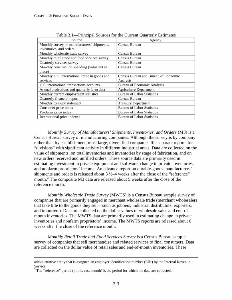
CHAPTER 3: PRINCIPAL SOURCE DATA

3-3

Table 3.1—Principal Sources for the Current Quarterly Estimates

Source Agency Monthly survey of manufacturers’ shipments, inventories, and orders

Census Bureau

Monthly wholesale trade survey Census Bureau Monthly retail trade and food services survey Census Bureau Quarterly services survey Census Bureau Monthly construction spending (value put in place)

Census Bureau

Monthly U.S. international trade in goods and services

Census Bureau and Bureau of Economic Analysis

U.S. international transactions accounts Bureau of Economic Analysis Annual projections and quarterly farm data Agriculture Department Monthly current employment statistics Bureau of Labor Statistics Quarterly financial report Census Bureau Monthly treasury statement Treasury Department Consumer price index Bureau of Labor Statistics Producer price index Bureau of Labor Statistics International price indexes Bureau of Labor Statistics

Monthly Survey of Manufacturers’ Shipments, Inventories, and Orders (M3) is a Census Bureau survey of manufacturing companies. Although the survey is by company rather than by establishment, most large, diversified companies file separate reports for “divisions” with significant activity in different industrial areas. Data are collected on the value of shipments, on total inventories and inventories by stage of fabrication, and on new orders received and unfilled orders. These source data are primarily used in estimating investment in private equipment and software, change in private inventories, and nonfarm proprietors’ income. An advance report on durable-goods manufacturers’ shipments and orders is released about 3 ½–4 weeks after the close of the “reference” month.3 The composite M3 data are released about 5 weeks after the close of the reference month. Monthly Wholesale Trade Survey (MWTS) is a Census Bureau sample survey of companies that are primarily engaged in merchant wholesale trade (merchant wholesalers that take title to the goods they sell—such as jobbers, industrial distributors, exporters, and importers). Data are collected on the dollar values of wholesale sales and end-of-month inventories. The MWTS data are primarily used in estimating change in private inventories and nonfarm proprietors’ income. The MWTS reports are released about 6 weeks after the close of the reference month. Monthly Retail Trade and Food Services Survey is a Census Bureau sample survey of companies that sell merchandise and related services to final consumers. Data are collected on the dollar value of retail sales and end-of-month inventories. These

administrative entity that is assigned an employer identification number (EIN) by the Internal Revenue Service. 3 The “reference” period (in this case month) is the period for which the data are collected.

CHAPTER 3: PRINCIPAL SOURCE DATA

3-4

source data are primarily used in estimating personal consumption expenditures (PCE) and change in private inventories. An advance report on monthly sales for retail and food services (MARTS) is released about 1 ½–2 weeks after the close of the reference month. The composite retail sales and inventories data are released about 6 weeks after the close of the reference month. Quarterly Services Survey (QSS) is a Census Bureau sample survey that was initiated in 2003–2004 in order to improve the coverage of the service industries in the U.S. economy. The coverage of the QSS has since been expanded several times so that it now covers most of the categories of health care, transportation services, recreation services, communication services, and professional and other services.4 The QSS data are primarily used in estimating PCE and investment in private equipment and software. The QSS data are released about 2 ½ months after the close of the reference quarter. Monthly construction spending (value put-in-place) is a Census Bureau measure of the value of construction installed or erected during a given period. The data for private nonresidential buildings, for government structures, and for multifamily residential buildings are derived from data collected by sampling the owners of construction projects.5 The data for single-family residential buildings are derived indirectly using information collected in a series of sample surveys that track the number of housing-unit permits, starts, sales, and completions. The data for “other construction” are derived from a variety of sources covering farm, utility, communication, and railroad structures. These source data are primarily used in estimating private and government investment in structures. The data for construction put-in-place are released about 1 month after the close of the reference month. Monthly U.S. international trade in goods and services consist of Census Bureau estimates of trade in goods and BEA estimates of trade in services. The Census Bureau tabulations of exported and imported goods are from documents filed with Customs and Border Protection, U.S. Department of Homeland Security; they cover all shipments above a certain size and a sample of the remaining shipments. The BEA estimates are primarily based on 11 mandatory BEA surveys of selected services receipts, payments, and other data. These data are supplemented by a combination of monthly indicator source data, partial data from U.S. government agencies and from foreign central statistical offices and banks, and other secondary source data. These source data are primarily used in estimating private investment in equipment and software and in estimating exports and imports. The U.S. international trade statistics are jointly released by the two agencies 6-7 weeks after the close of the reference month. 4 For a discussion of the newly available QSS data for 2011, see Eugene P. Seskin and Alyssa E. Holdren, “Annual revision of the National Income and Product Accounts,” Survey of Current Business 92 (August 2012): 24. 5 In contrast, the census of construction, which is part of the economic census, measures construction on the basis of reports by establishments primarily engaged in construction. Thus, value put-in-place captures some important parts of construction activity that are not included in the census—such as nonemployer construction, architectural and engineering costs, own-account construction, homeowner construction, and construction done as a secondary source of revenue by nonconstruction establishments.

CHAPTER 3: PRINCIPAL SOURCE DATA

3-5

International Transactions Accounts (ITAs), prepared by BEA, summarize the quarterly transactions between the United States and the rest of the world. In the ITAs, the current account records exports and imports of goods and services, receipts and payments of income on assets, and unilateral transfers (net gifts to other countries). In the capital and financial account, the capital account records capital transfers (such as debt forgiveness) and the financial account records transactions involving exchanges of financial assets for other financial assets or for tangible resources and gifts or grants of financial assets. These source data are primarily used in estimating corporate profits. The ITAs are released about 2½ months after the close of the reference quarter. Annual projections and quarterly farm data, from the U.S. Department of Agriculture, consist of annual projections of crop output, quarterly projections of cash receipts and of inventories for livestock, and annual projections of government subsidy payments and production expenses for both crops and livestock. These data are primarily used in estimating change in private inventories and farm proprietors’ income. Monthly Current Employment Statistics (CES) survey is a sample survey of business establishments that is conducted by state employment security agencies in cooperation with BLS. The CES (also known as BLS-790) covers payroll employment in private nonagricultural industries during the pay period that includes the 12th of the month. The data collected include series for total employment, number of production or nonsupervisory workers, average hourly earnings, average weekly hours, average weekly earnings, and average weekly overtime hours in manufacturing industries. (BLS has developed experimental series that extend coverage to all employees and that include irregular payments, such as bonuses.) These source data are primarily used in estimating PCE, wages and salaries, and nonfarm proprietors’ income. The CES data are usually released on the first Friday following the close of the reference month. Quarterly Financial Report (QFR), prepared by the Census Bureau, provides aggregate statistics on the financial position of U.S. corporations. Based on a sample survey of firms above specified asset sizes, the QFR presents estimated statements of income and retained earnings, balance sheets, and related financial and operating ratios for manufacturing, mining, and trade corporations by industry and by asset size. These source data are primarily used in estimating corporate profits. The QFR statistics for manufacturing, mining, and wholesale trade are released about 2 ½ months after the close of the reference quarter, and the statistics for retail trade are released about 1 month later. Monthly Treasury Statement (MTS), prepared by the Financial Management Service of the U.S. Department of the Treasury, summarizes the financial activities of the federal government and off-budget federal entities in accordance with the Budget of the U.S. Government. The MTS presents a summary of receipts and outlays, surplus or deficit, and means of financing. The data are provided by federal entities, disbursing officers, and Federal Reserve Banks. These source data are primarily used in estimating federal government receipts and expenditures and federal government consumption expenditures and gross investment. The MTS is released about 2 weeks after the close of the reference month.

CHAPTER 3: PRINCIPAL SOURCE DATA

3-6

Consumer Price Index (CPI), prepared by BLS, is a family of indexes that measure the average monthly change in the prices paid by urban consumers for a fixed market basket of goods and services. The CPI covers “out-of-pocket” expenditures, including user fees (such as water and sewer service) and sales and excise taxes paid by the consumer but excluding income taxes and investment items (such as stocks, bonds, and life insurance). The CPI is estimated from a statistical set of samples of urban areas, of consumers within those areas, of retailers and other outlets, and of specific, unique items purchased. CPIs are primarily used in deflating PCE, change in private inventories, and state and local government purchases. The CPI is released 2–3 weeks after the close of the reference month. Producer Price Index (PPI), prepared by BLS, is a family of indexes that measure the average monthly change in prices received by domestic producers of goods and services. Thus, the PPI measures price change from the perspective of the seller rather than the purchaser. The PPI covers practically the entire output of domestic goods-producing sectors and is expanding its coverage of services and other non-goods-producing sectors. The PPI is estimated from data collected from a sample of establishments that participate in the Unemployment Insurance System, a joint federal and state program that covers about 97 percent of wage and salary workers. PPIs are primarily used in deflating private investment in equipment and software and in structures, change in private inventories, government purchases, and exports and imports. The PPI is released about 2 weeks after the close of the reference month.

International Price Indexes, prepared by BLS, measure monthly changes in the prices of goods and services that are sold by U.S. producers to foreign buyers (exports) and that are purchased from abroad by U.S. buyers (imports). The price indexes for exports of goods to Canada are based primarily on sampling information obtained from the Canadian Customs Service, and the indexes for exports of goods to other countries are based on sampling information obtained from the U.S. Census Bureau. The price indexes for imports of goods are based on sampling information obtained from Customs and Border Protection, U.S. Department of Homeland Security. The price indexes for exports and imports of services are based on sampling information that is developed separately for each service category. These price indexes are primarily used in deflating private investment in equipment and software, change in private inventories, and exports and imports. The international price indexes are released about 2 weeks after the close of the reference month. Estimating schedule For GDP and most other NIPA series, the estimates for each quarter are prepared on a schedule that calls for three successive "current" estimates—"advance," "second," and "third."6 The specific release date for each month is primarily determined by the

6 In the 2009 comprehensive revision of the NIPAs, BEA introduced new names for the second two vintages of the current quarterly estimates. Formerly, the “second” estimate was known as the “preliminary” estimate, and the “third” estimate” was known as the “final” estimate. The initial estimate

CHAPTER 3: PRINCIPAL SOURCE DATA

3-7

availability of the monthly reports on retail sales, manufacturing shipments, and international trade in goods from the Census Bureau (along with the time it takes BEA to process them).

• The advance quarterly estimate of GDP is released near the end of the month that follows the close of the reference quarter. For most of the product-side components, the estimate is based on source data for either 2 or 3 months of the quarter. In most cases, however, the source data for the second and third months of the quarter are subject to revision by the issuing agencies. Where source data are not available, the estimate is based primarily on BEA projections. For an example of how this information is provided in the Survey of Current Business, see the box “Source Data and Key Assumptions for the Advance Estimates of GDP for the Second Quarter of 2012” on the next page (which was adapted from “GDP and the Economy” in the August 2012 Survey).

• One month later, the advance estimate is replaced by the second estimate, which is typically based on source data for all 3 months of the quarter. However, in some instances, the source data used for the second estimate, particularly the data for the third month of the quarter, are subject to further revision.

• One month later, the second estimate is replaced by the third estimate, which incorporates revisions to source data for the third month of the quarter and newly available quarterly source data for some components.

For certain “income-side” series—gross national product, gross domestic income,

national income, and corporate profits—“advance” estimates are not prepared, because of a lag in the availability of source data. For the first, second, and third quarters of the year, the release of the second GDP estimate presents the initial estimates for these income-side series, and the third GDP release presents revised estimates. For the fourth quarter, the estimates for these series are presented only in the third GDP release.

In addition, when the second estimate of GDP for the current quarter is released,

the preceding quarter’s estimates of private wages and salaries and affected income-side aggregates are revised to incorporate newly available preliminary tabulations from the BLS quarterly census of employment and wages (QCEW).7 (For a description of the QCEW, see the section on source data for annual revisions.)

continues to be named the “advance” estimate. (See Eugene P. Seskin and Shelly Smith, “Preview of the 2009 Comprehensive Revision of the NIPAs: Changes in Definitions and Presentations,” Survey of Current Business 89 (March 2009): 19–20.) 7 Affected aggregates include gross domestic income, the statistical discrepancy, gross national income, national income, personal income, disposable personal income, personal saving, gross (national) saving, compensation, and gross product of corporate business. Other components that are closely linked to wages and salaries, such as personal current taxes and employer contributions for government social insurance, are also revised. Product-side series, including GDP, are not affected.

CHAPTER 3: PRINCIPAL SOURCE DATA

3-8

Source Data and Key Assumptions for the Advance Estimates of GDP for the Second Quarter of 2012

The advance estimates of many components of GDP are based on 3 months of

source data, but the estimates of some components are based on only 2 months of data. For the following items, the number of months for which source data are available is shown in parentheses. Personal consumption expenditures: sales of retail stores (3), unit auto and truck sales (3), consumer’ shares of auto and truck sales (2), gasoline (2), and utilities (2); Nonresidential fixed investment: unit auto and truck sales (3), construction spending (value put in place) (2), manufacturers’ shipments of machinery and equipment (3), and exports and imports of machinery and equipment (2); Residential fixed investment: construction spending (value put in place) (2), single-family housing starts (3), sales of new homes (2), and sales of existing houses (3); Change in private inventories: trade and nondurable-goods manufacturing inventories (2), durable-goods manufacturing inventories (3), and unit auto and truck inventories (3); Net exports of goods and services: exports and imports of goods and services (2); Government consumption expenditures and gross investment: federal outlays (3), state and local construction spending (value put in place) (2), and state and local government employment (3); Compensation: employment, average hourly earnings, and average weekly hours (3); and Prices: consumer price indexes (3), producer price indexes (3), and values and quantities of petroleum imports (2). Unavailable source data When source data were unavailable, BEA made various assumptions for June, including the following:

• A decrease in nonresidential structures, • Increases in both single-family and multifamily residential structures, • A decrease in change in inventories of nondurable-goods manufacturing

industries and an increase in the change in nonmotor vehicle merchant wholesale and retail trade inventories,

• A small decrease in exports of goods excluding gold and a somewhat larger decrease in imports excluding gold, and

CHAPTER 3: PRINCIPAL SOURCE DATA

3-9

Source-data categories The source data used to prepare the quarterly estimates of the product-side components of GDP can be grouped into four general categories based on their quality, availability, and use.8

• Revised monthly or quarterly data are based on revised monthly or quarterly source data; they are presumed to be more accurate than preliminary data.

• Initial monthly or quarterly data include either monthly data for all 3 months of a quarter or data for a complete quarter.

• Monthly data and trend-based data typically include source data for the first 2 months but limited or no data for the third month; for the third month, BEA makes a projection based on various assumptions.

• Trend-based data are typically projections that are calculated by BEA using previous estimates and trends, moving averages of various lengths, regressions, and judgment by BEA economists.

For the advance GDP estimate, initial monthly or quarterly data account for 46

percent of the source data used to calculate the estimates. Monthly data and trend-based data account for 30 percent, and trend-based data account for the remainder. (See chart 3.1 on the next page).

For the second and third GDP estimates, most of the monthly data and trend-based data are replaced by revised monthly or quarterly data, which are generally considered more accurate. The revised data account for 72 percent of the source data for those estimates. For the second estimate, most of the remainder is accounted for by trend-based data, at 24 percent. For the third estimate, however, most of the remainder is accounted for by initial monthly or quarterly data, at 20 percent.

The estimates of new residential structures provide an example of the progression

of source data from the advance quarterly estimate to the third quarterly estimate. The advance estimate of new residential structures incorporates source data for the first and second months of the quarter and an assumption for the third month; these source data are categorized as monthly data and trend-based data. The second estimate incorporates revised data for the first and second months and newly available data for the third month; these source data are categorized as revised monthly or quarterly data. The third estimate incorporates data for the second and third months that are revised further; these source data are also categorized as revised monthly or quarterly data.

8 For more information, see Bruce T. Grimm and Teresa L. Weadock, “Gross Domestic Product: Revisions and Source Data,” Survey 86 (February 2006): 11–15.

CHAPTER 3: PRINCIPAL SOURCE DATA

3-10

Chart 3.1— Shares of Source Data for the Quarterly GDP Estimates

Source data for the annual revisions

Annual revisions of the NIPAs are usually released in July and cover the months and quarters of the most recent calendar year and of the 2 preceding years.9 The NIPA estimates for the most recent calendar year are revised to incorporate revisions that result from annual benchmarking of some of the principal monthly or quarterly source data. The NIPA estimates for all 3 years are revised to incorporate a broad range of newly available and revised annual source data (table 3.2). For the expenditures components, the newly available source data include annual surveys conducted by the Census Bureau. For the income components, the newly available source data include IRS tabulations of income tax returns and BLS tabulations of employment and wage information.

9 Starting in 2010, BEA instituted a “flexible” approach to annual revisions that allows for the incorporation of improvements in methodology and for the extension of the 3-year revision period to earlier periods; see “BEA Briefing: Improving BEA’s Accounts Through Flexible Annual Revisions,” Survey 88 (June 2008): 29–32.

ADVANCE ESTIMATE

Trend-based data 23.7%

Monthly and trend-based data 30.1%

Initial monthly or quarterly data

46.2%

SECOND ESTIMATE

Trend-based data 23.7%

Monthly and trend-based data

0.4%

Revised data 71.7%

Initial monthly or quarterly data

4.2%

THIRD ESTIMATE

Trend-based data 8.5%

Revised data 71.7%

Initial monthly or quarterly data

19.8%

FIRST ANNUAL ESTIMATE

Revised data 45.1%Annual data

52.6%

Trend-based data 2.3%

CHAPTER 3: PRINCIPAL SOURCE DATA

3-11

Table 3.2—Principal Newly Available Sources for NIPA Annual Revisions Source Agency

Annual survey of manufactures Census Bureau Annual wholesale trade survey Census Bureau Annual retail trade survey Census Bureau Service annual survey Census Bureau Annual surveys of state and local government finances

Census Bureau

Annual revision of the international transactions accounts

Bureau of Economic Analysis

Annual farm statistics Agriculture Department Quarterly census of employment and wages Bureau of Labor Statistics Tabulations of tax returns Internal Revenue Service Federal government annual budget Office of Management and Budget

The first four sources listed in table 3.2 are the annual counterparts of the Census Bureau monthly surveys used for the current quarterly estimates. The more extensive annual survey samples are from companies listed in the Business Register, and the recipients are selected by stratified probability sampling. Response to these surveys is mandatory. New samples are usually selected after each economic census, and the samples are updated periodically to reflect business “births” and “deaths.” Annual Survey of Manufactures (ASM) is a Census Bureau survey of manufacturing establishments with paid employees. The ASM is conducted in the years between the economic census—that is, in all years not ending in 2 or 7. Data are collected on employment, payroll, value added by manufacture, materials consumed, value of shipments, detailed capital expenditures, supplemental labor costs, fuels and electric energy used, and inventories by stage of fabrication. These source data are primarily used in estimating private investment in equipment and software, change in private inventories, and nonfarm proprietors’ income. The ASM data are published about 11 months after the close of the reference year. Annual Wholesale Trade Survey (AWTS) is a Census Bureau survey of companies that have significant activity in wholesale trade. These companies include wholesalers that take title of the goods they sell—such as jobbers, industrial distributors, exporters, importers, and manufacturer sales branches and offices (MSBOs)—and, beginning in 2007, wholesalers that do not take title—such as agents, merchandise and commodity brokers, commission merchants, and electronic business-to-business marketers. Merchant wholesalers excluding MSBOs provide data on sales, inventories, inventory valuation, purchases, and gross margin. MSBOs provide data on sales, inventories, inventory valuation, and operating expenses. The wholesalers that do not take title provide data on sales, commissions earned, gross selling value of sales conducted for others, and operating expenses. The AWTS data are primarily used in estimating change in private inventories and nonfarm proprietors’ income. The statistics for all wholesalers are normally published about 15 months following the close of the reference year.

CHAPTER 3: PRINCIPAL SOURCE DATA

3-12

Annual Retail Trade Survey (ARTS) is a Census Bureau survey of retail companies with one or more establishments that sell merchandise and associated services to final consumers. The survey is sent to a sample of retail establishments with paid employees, and the data collected are supplemented by administrative data to account for businesses without paid employees. The ARTS collects data on the dollar value of retail sales, sales taxes collected, inventories, inventory valuation, cost of purchases, and accounts receivables balances. These source data are primarily used in estimating PCE and change in private inventories. The statistics are normally published about 15 months following the close of the reference year. Service Annual Survey (SAS) is a Census Bureau survey of companies that provide services to individuals, businesses, and governments. The survey is sent to selected businesses with paid employees, and the data collected are supplemented by administrative data or imputed values to account for businesses without paid employees and for certain other businesses. The data collected include operating revenue for both taxable and tax-exempt firms and organizations, sources of revenue, exports, and inventories for selected industries, and selected industry-specific items. The SAS has been expanded over time in order to in order to improve the coverage of the service industries in the U.S. economy.10 The SAS data are primarily used in estimating PCE and private investment in equipment and software. The statistics are normally published about 12 months after the close of the reference year. Annual surveys of state and local government finances, prepared by the Census Bureau, provide data on the financial activities of state governments and of local governments, including counties, municipalities, townships, special districts, and school districts. The data are compiled from three sources: an enumeration of all 50 states, a probability sample survey of local governments, and data from federal government agencies. Reported data are for each government’s annual accounting period (fiscal year) that ends on or before June 30 of the survey year. Data are obtained for revenue, expenditure, debt, and financial assets. These source data are primarily used in estimating state and local government spending, employee compensation, and taxes on production and imports. The data are available about 12 months after the close of the survey year. Annual revision of the international transactions accounts (ITAs), prepared by BEA, incorporates newly available annual source data and statistical, methodological, and presentational improvements into the accounts, which may result in revisions that extend back for a number of years.11 (The ITAs were described in the preceding section on sources for the current quarterly estimates.) These source data are primarily used in estimating private investment in equipment and software, exports of goods and services, and imports of goods and services. The annual revision of the ITAs is released in mid-June.

10 For a discussion of the most recent expansion of the SAS, see Eugene P. Seskin and Alyssa E. Holdren, 24. 11 For a description of an annual revision of the ITAs, see the most recent July issue of the Survey.

CHAPTER 3: PRINCIPAL SOURCE DATA

3-13

Annual farm statistics are collected in the Agricultural Resource Management Survey (ARMS), which is sponsored jointly by the Economic Research Service and the National Agricultural Statistics Service of the U.S. Department of Agriculture. The ARMS starts in the fall with the collection of data on crop production and costs and finishes in the spring with the collection of data on whole farm and livestock production practices and costs. The data, which underpin USDA’s annual estimates of net farm income, cover virtually every aspect of U.S. agriculture, including production and supplies, prices paid and received, farm labor and wages, and farm finances. These source data are primarily used in estimating change in private inventories and farm proprietors’ income. The ARMS data are available in the fall following the close of the reference year. Quarterly Census of Employment and Wages (QCEW) is a cooperative program (also known as the ES-202 program) involving BLS and the state employment security agencies. The QCEW produces a comprehensive tabulation of employment and wage information for workers who are covered by state unemployment insurance programs or by the unemployment insurance program for federal employees; these workers represent over 95 percent of civilian wage and salary employment. These source data are primarily used in estimating PCE, wages and salaries, and nonfarm proprietors’ income. The QCEW data are usually released to the public 6 to 7 months after the close of the reference quarter.12 Tabulations of tax returns, prepared by the IRS Statistics of Income program, are compilations of information from the tax returns of corporations and of sole proprietorships and partnerships. The aggregate data are compiled based on stratified probability samples of tax or information returns. The data collected include by-industry information on assets, business receipts and deductions, and net income. The source data are primarily used in estimating corporate profits and nonfarm proprietors’ income. The data for nonfarm sole proprietorships and partnerships are released to the public about 1 ½–1 ¾ years after the end of the tax year, and the data for corporations are released to the public about 1 ¾ years after the end of the tax year.13 Federal government annual budget, a report prepared by the Office of Management and Budget, presents preliminary estimates of U.S. Government receipts and expenditures for the current fiscal year (October 1 through September 30) and revised data for the preceding fiscal year, as well as the President’s proposed budget for the upcoming fiscal year. Data are provided on budget receipts by source, such as individual and corporate income taxes, and on budget outlays by function, such as national defense and Medicare. These source data are primarily used in estimating federal

12 As noted in footnote 6, some preliminary information from the QCEW is incorporated into the quarterly estimates on a delayed basis. However, the annual NIPA revision provides the opportunity for a more complete incorporation of these data. 13 For corporations, the tax year covers tax returns that are filed for accounting periods ending in July of one year through June of the following year; for most corporations, the accounting period coincides with the calendar year.

CHAPTER 3: PRINCIPAL SOURCE DATA

3-14

government spending and wages and salaries. The report is usually released in early February.

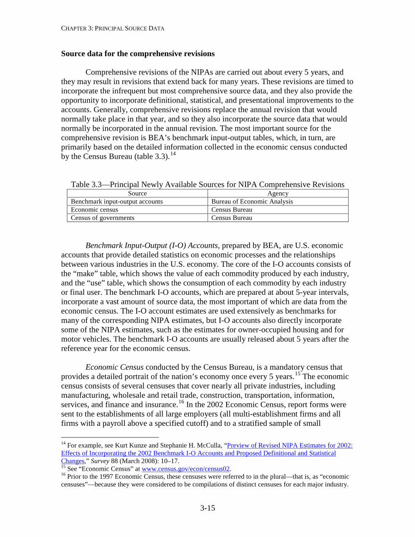
CHAPTER 3: PRINCIPAL SOURCE DATA

3-15

Source data for the comprehensive revisions

Comprehensive revisions of the NIPAs are carried out about every 5 years, and they may result in revisions that extend back for many years. These revisions are timed to incorporate the infrequent but most comprehensive source data, and they also provide the opportunity to incorporate definitional, statistical, and presentational improvements to the accounts. Generally, comprehensive revisions replace the annual revision that would normally take place in that year, and so they also incorporate the source data that would normally be incorporated in the annual revision. The most important source for the comprehensive revision is BEA’s benchmark input-output tables, which, in turn, are primarily based on the detailed information collected in the economic census conducted by the Census Bureau (table 3.3).14

Table 3.3—Principal Newly Available Sources for NIPA Comprehensive Revisions Source Agency

Benchmark input-output accounts Bureau of Economic Analysis Economic census Census Bureau Census of governments Census Bureau

Benchmark Input-Output (I-O) Accounts, prepared by BEA, are U.S. economic accounts that provide detailed statistics on economic processes and the relationships between various industries in the U.S. economy. The core of the I-O accounts consists of the “make” table, which shows the value of each commodity produced by each industry, and the “use” table, which shows the consumption of each commodity by each industry or final user. The benchmark I-O accounts, which are prepared at about 5-year intervals, incorporate a vast amount of source data, the most important of which are data from the economic census. The I-O account estimates are used extensively as benchmarks for many of the corresponding NIPA estimates, but I-O accounts also directly incorporate some of the NIPA estimates, such as the estimates for owner-occupied housing and for motor vehicles. The benchmark I-O accounts are usually released about 5 years after the reference year for the economic census. Economic Census conducted by the Census Bureau, is a mandatory census that provides a detailed portrait of the nation’s economy once every 5 years.15 The economic census consists of several censuses that cover nearly all private industries, including manufacturing, wholesale and retail trade, construction, transportation, information, services, and finance and insurance.16 In the 2002 Economic Census, report forms were sent to the establishments of all large employers (all multi-establishment firms and all firms with a payroll above a specified cutoff) and to a stratified sample of small

14 For example, see Kurt Kunze and Stephanie H. McCulla, “Preview of Revised NIPA Estimates for 2002: Effects of Incorporating the 2002 Benchmark I-O Accounts and Proposed Definitional and Statistical Changes,” Survey 88 (March 2008): 10–17. 15 See “Economic Census” at www.census.gov/econ/census02. 16 Prior to the 1997 Economic Census, these censuses were referred to in the plural—that is, as “economic censuses”—because they were considered to be compilations of distinct censuses for each major industry.

CHAPTER 3: PRINCIPAL SOURCE DATA

3-16

employers (single-establishment firms with payroll below the cutoff). Statistics for selected small employers (for example, those with fewer than 10 employees) and all firms without employees were compiled from administrative records of the IRS and other federal government agencies. The economic census is the most important data source for the benchmark I-O accounts. Results from the economic census are released over a period of several years. Census of Governments, which is conducted by the Census Bureau in the same years as the economic census, is a voluntary census that provides periodic and comprehensive statistics about governments and governmental activities. The census covers all state and local governments, including counties, cities, townships, special districts, and school districts. Data are collected on revenues, expenditures, debt, assets, employees, payroll, and benefits for the individual fiscal year that ended prior to July 1 of the census year. These source data are primarily used in estimating state and local government spending. The financial data are released beginning about 16 months after the close of the census year, and the employment data are released beginning about 12 months after the close of the census year.

4-1

CHAPTER 4: ESTIMATING METHODS (Updated: November 2012)

Current-Dollar Estimates Adjustments to the source data Seasonal adjustment Moving average Best level and best change Interpolation and extrapolation using an indicator series Three special estimation methods Commodity-flow method Retail control method Perpetual inventory method Quantity and Price Estimates Estimates for detailed components Estimates for NIPA aggregates Properties of chain-type measures Appendix to Chapter 4

Calculating Output and Price Indexes Statistical Tools and Conventions

Chained-dollar measures Contributions to percent change Annual rates Growth rates Rebasing an index The NIPA measures are built up from a wide range of source data using a variety of estimating methods. Each NIPA component is derived using a specific methodology—that is, source data and estimating methods—that progresses from the advance quarterly estimate through the comprehensive NIPA revision. The methodologies used to prepare the various NIPA estimates are periodically changed in order to incorporate improvements in the source data or in the estimating methods.1

• Over time, source data may emerge or disappear, so new source data must be identified and evaluated, and estimating methods must be adapted accordingly.

• Advances in statistical techniques or in other aspects of estimation must be evaluated for adoption into the methodology.

• As the U.S. economy evolves, the methodology must be updated to ensure that the estimates continue to provide a reliable and relevant picture of transactions and transactors in the economy.

1 Substantive changes to NIPA methodologies are documented in BEA’s monthly Survey of Current Business.

CHAPTER 4: ESTIMATING METHODS

4-2

The examples provided in this chapter are simplified in order to illustrate the basic estimating concepts and calculations. In practice, the procedures used for deriving the NIPAs involve complex statistical techniques that are designed to ensure consistency across the entire time series for a given estimate and between interrelated estimates.

Current-Dollar Estimates For most NIPA components, the current-dollar, or nominal, estimates are derived from source data that are “value data,” which reflect the product of quantity and price. For the estimates that are not derived from value data, separate quantity data and price data must be combined. For example, an estimate of expenditures on new autos may be calculated as the number of autos sold times expenditure per auto (at transaction prices—that is, the average list price with options adjusted for transportation charges, sales taxes, dealer discounts, and rebates). An estimate of wages may be calculated as employment times average hourly earnings times average hours worked, and an estimate of interest received may be calculated as the stock of interest-bearing assets times an effective interest rate. (The NIPA current-dollar estimates are expressed at annual rates; see the appendix to this chapter.) Adjustments to the source data

BEA makes three general types of adjustments to the source data that are incorporated into the NIPA estimates. The first consists of adjustments that are needed so that the data conform to appropriate NIPA concepts and definitions. For example, Internal Revenue Service data from corporate tax returns include estimates of depreciation, but these estimates are based on historical-cost valuation and on tax service lives. BEA must adjust these estimates to the NIPA definition of depreciation—consumption of fixed capital—which is based on current-cost valuation and economic service lives.

The second type of adjustment involves filling gaps in coverage. For example,

one of the primary sources for the quarterly estimates of the change in private inventories component of GDP is the Census Bureau’s monthly survey of wholesale trade. However, this source does not cover inventories of nonmerchant wholesalers (wholesalers that do not take title to the goods they sell). Thus, the survey data must be augmented by separate BEA estimates for the change in the inventories of these wholesalers.

The third type of adjustment involves time of recording and valuation. For

example, in the NIPAs (as in BEA’s international transactions accounts), imported goods are valued at “foreign port value”—that is, the value at the point of exportation to the United States. The source data on imports of goods from Canada, which the Census Bureau receives in a bilateral data exchange with Canada, are often valued at the point of manufacture; thus, BEA must adjust these data to foreign port value by adding the cost of

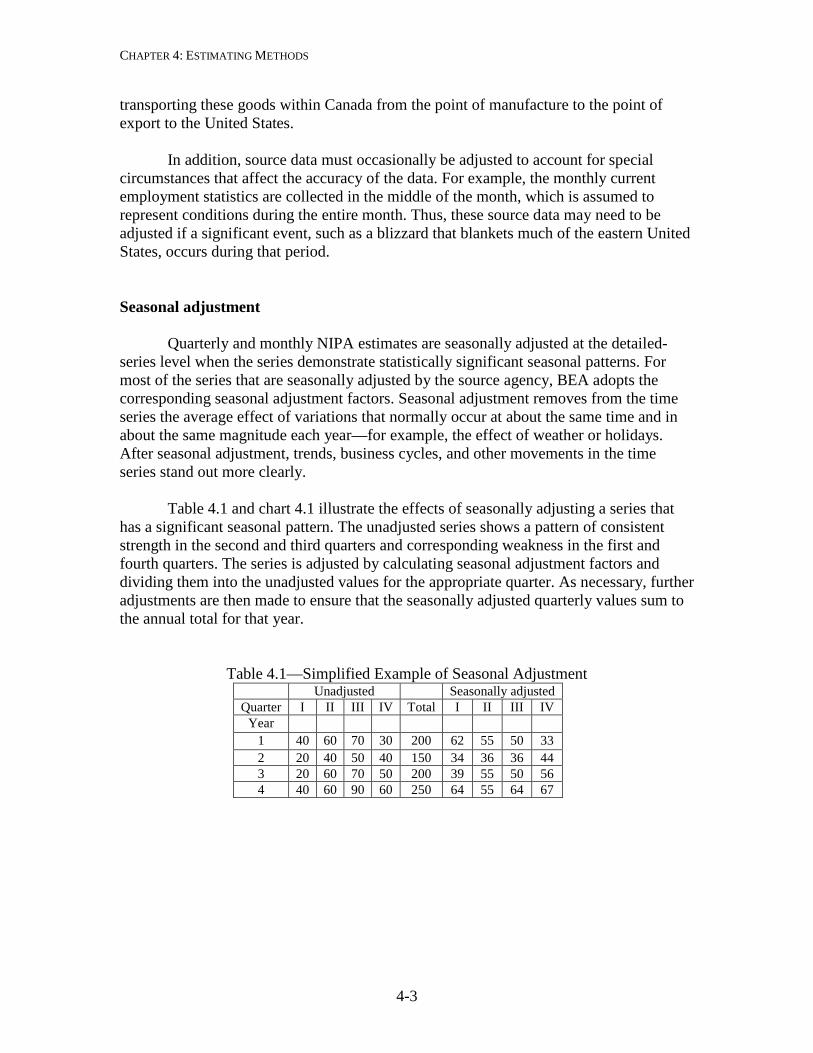
CHAPTER 4: ESTIMATING METHODS

4-3

transporting these goods within Canada from the point of manufacture to the point of export to the United States. In addition, source data must occasionally be adjusted to account for special circumstances that affect the accuracy of the data. For example, the monthly current employment statistics are collected in the middle of the month, which is assumed to represent conditions during the entire month. Thus, these source data may need to be adjusted if a significant event, such as a blizzard that blankets much of the eastern United States, occurs during that period. Seasonal adjustment

Quarterly and monthly NIPA estimates are seasonally adjusted at the detailed-series level when the series demonstrate statistically significant seasonal patterns. For most of the series that are seasonally adjusted by the source agency, BEA adopts the corresponding seasonal adjustment factors. Seasonal adjustment removes from the time series the average effect of variations that normally occur at about the same time and in about the same magnitude each year—for example, the effect of weather or holidays. After seasonal adjustment, trends, business cycles, and other movements in the time series stand out more clearly. Table 4.1 and chart 4.1 illustrate the effects of seasonally adjusting a series that has a significant seasonal pattern. The unadjusted series shows a pattern of consistent strength in the second and third quarters and corresponding weakness in the first and fourth quarters. The series is adjusted by calculating seasonal adjustment factors and dividing them into the unadjusted values for the appropriate quarter. As necessary, further adjustments are then made to ensure that the seasonally adjusted quarterly values sum to the annual total for that year.

Table 4.1—Simplified Example of Seasonal Adjustment

Unadjusted Seasonally adjusted Quarter I II III IV Total I II III IV

Year 1 40 60 70 30 200 62 55 50 33 2 20 40 50 40 150 34 36 36 44 3 20 60 70 50 200 39 55 50 56 4 40 60 90 60 250 64 55 64 67

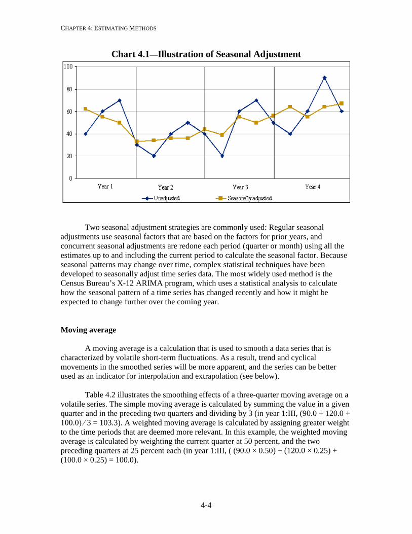
CHAPTER 4: ESTIMATING METHODS

4-4

Chart 4.1—Illustration of Seasonal Adjustment

Two seasonal adjustment strategies are commonly used: Regular seasonal adjustments use seasonal factors that are based on the factors for prior years, and concurrent seasonal adjustments are redone each period (quarter or month) using all the estimates up to and including the current period to calculate the seasonal factor. Because seasonal patterns may change over time, complex statistical techniques have been developed to seasonally adjust time series data. The most widely used method is the Census Bureau’s X-12 ARIMA program, which uses a statistical analysis to calculate how the seasonal pattern of a time series has changed recently and how it might be expected to change further over the coming year. Moving average A moving average is a calculation that is used to smooth a data series that is characterized by volatile short-term fluctuations. As a result, trend and cyclical movements in the smoothed series will be more apparent, and the series can be better used as an indicator for interpolation and extrapolation (see below). Table 4.2 illustrates the smoothing effects of a three-quarter moving average on a volatile series. The simple moving average is calculated by summing the value in a given quarter and in the preceding two quarters and dividing by 3 (in year 1:III, (90.0 + 120.0 + 100.0) ∕ 3 = 103.3). A weighted moving average is calculated by assigning greater weight to the time periods that are deemed more relevant. In this example, the weighted moving average is calculated by weighting the current quarter at 50 percent, and the two preceding quarters at 25 percent each (in year 1:III, ( (90.0 × 0.50) + (120.0 × 0.25) + (100.0 × 0.25) = 100.0).

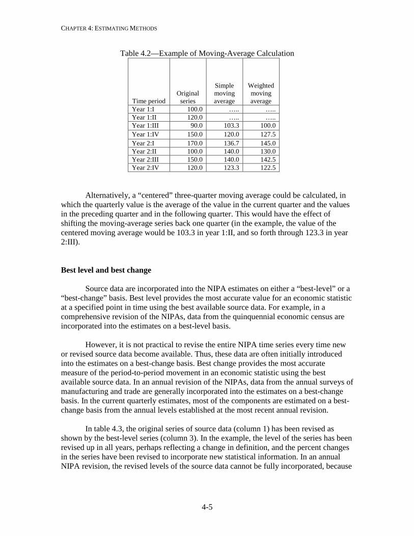
CHAPTER 4: ESTIMATING METHODS

4-5

Table 4.2—Example of Moving-Average Calculation

Time period Original

series

Simple moving average

Weighted moving average

Year 1:I 100.0 ….. ….. Year 1:II 120.0 ….. ….. Year 1:III 90.0 103.3 100.0 Year 1:IV 150.0 120.0 127.5 Year 2:I 170.0 136.7 145.0 Year 2:II 100.0 140.0 130.0 Year 2:III 150.0 140.0 142.5 Year 2:IV 120.0 123.3 122.5

Alternatively, a “centered” three-quarter moving average could be calculated, in which the quarterly value is the average of the value in the current quarter and the values in the preceding quarter and in the following quarter. This would have the effect of shifting the moving-average series back one quarter (in the example, the value of the centered moving average would be 103.3 in year 1:II, and so forth through 123.3 in year 2:III). Best level and best change Source data are incorporated into the NIPA estimates on either a “best-level” or a “best-change” basis. Best level provides the most accurate value for an economic statistic at a specified point in time using the best available source data. For example, in a comprehensive revision of the NIPAs, data from the quinquennial economic census are incorporated into the estimates on a best-level basis.

However, it is not practical to revise the entire NIPA time series every time new or revised source data become available. Thus, these data are often initially introduced into the estimates on a best-change basis. Best change provides the most accurate measure of the period-to-period movement in an economic statistic using the best available source data. In an annual revision of the NIPAs, data from the annual surveys of manufacturing and trade are generally incorporated into the estimates on a best-change basis. In the current quarterly estimates, most of the components are estimated on a best-change basis from the annual levels established at the most recent annual revision. In table 4.3, the original series of source data (column 1) has been revised as shown by the best-level series (column 3). In the example, the level of the series has been revised up in all years, perhaps reflecting a change in definition, and the percent changes in the series have been revised to incorporate new statistical information. In an annual NIPA revision, the revised levels of the source data cannot be fully incorporated, because

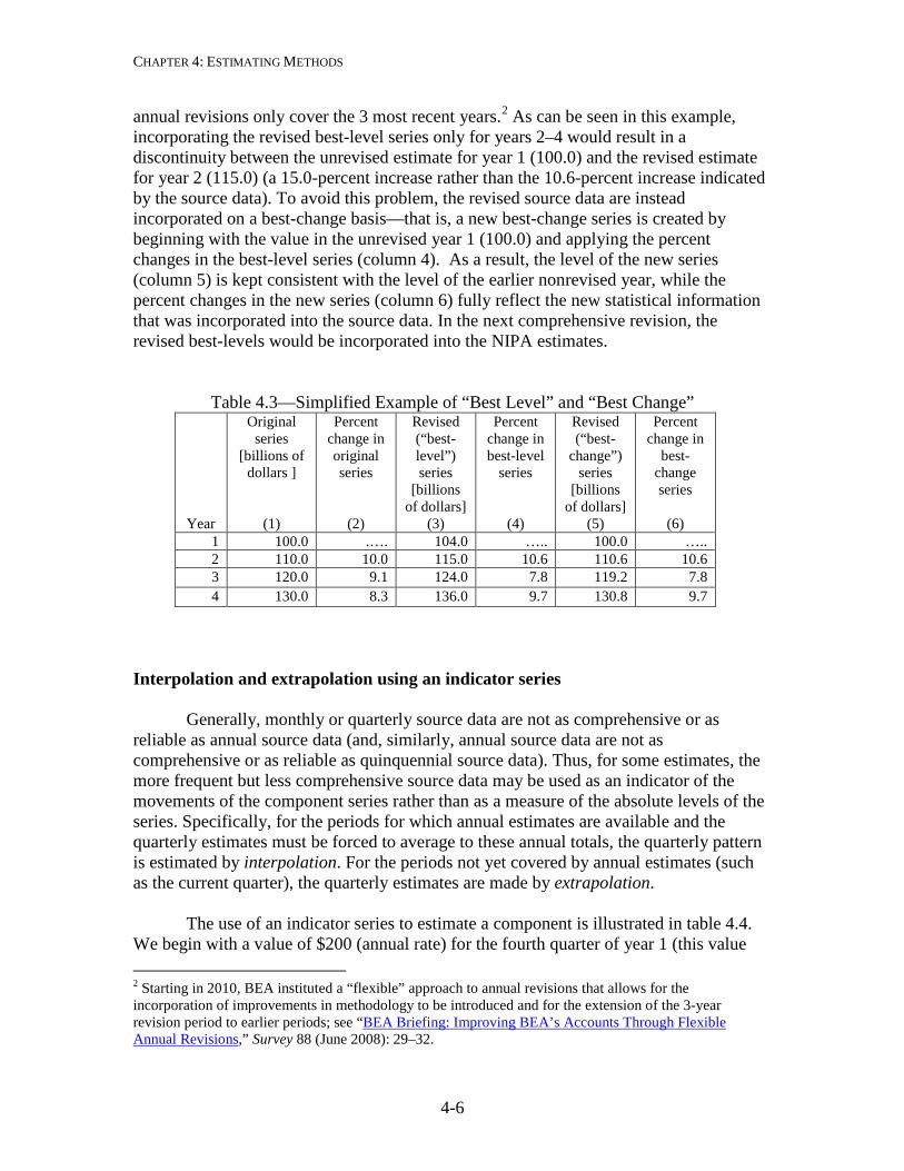
CHAPTER 4: ESTIMATING METHODS

4-6

annual revisions only cover the 3 most recent years.2 As can be seen in this example, incorporating the revised best-level series only for years 2–4 would result in a discontinuity between the unrevised estimate for year 1 (100.0) and the revised estimate for year 2 (115.0) (a 15.0-percent increase rather than the 10.6-percent increase indicated by the source data). To avoid this problem, the revised source data are instead incorporated on a best-change basis—that is, a new best-change series is created by beginning with the value in the unrevised year 1 (100.0) and applying the percent changes in the best-level series (column 4). As a result, the level of the new series (column 5) is kept consistent with the level of the earlier nonrevised year, while the percent changes in the new series (column 6) fully reflect the new statistical information that was incorporated into the source data. In the next comprehensive revision, the revised best-levels would be incorporated into the NIPA estimates.

Table 4.3—Simplified Example of “Best Level” and “Best Change”

Year

Original series

[billions of dollars ]

(1)

Percent change in original series

(2)

Revised (“best-level”) series

[billions of dollars]

(3)

Percent change in best-level

series

(4)

Revised (“best-

change”) series

[billions of dollars]

(5)

Percent change in

best-change series

(6)

1 100.0 .…. 104.0 ….. 100.0 ….. 2 110.0 10.0 115.0 10.6 110.6 10.6 3 120.0 9.1 124.0 7.8 119.2 7.8 4 130.0 8.3 136.0 9.7 130.8 9.7

Interpolation and extrapolation using an indicator series Generally, monthly or quarterly source data are not as comprehensive or as reliable as annual source data (and, similarly, annual source data are not as comprehensive or as reliable as quinquennial source data). Thus, for some estimates, the more frequent but less comprehensive source data may be used as an indicator of the movements of the component series rather than as a measure of the absolute levels of the series. Specifically, for the periods for which annual estimates are available and the quarterly estimates must be forced to average to these annual totals, the quarterly pattern is estimated by interpolation. For the periods not yet covered by annual estimates (such as the current quarter), the quarterly estimates are made by extrapolation. The use of an indicator series to estimate a component is illustrated in table 4.4. We begin with a value of $200 (annual rate) for the fourth quarter of year 1 (this value 2 Starting in 2010, BEA instituted a “flexible” approach to annual revisions that allows for the incorporation of improvements in methodology to be introduced and for the extension of the 3-year revision period to earlier periods; see “BEA Briefing: Improving BEA’s Accounts Through Flexible Annual Revisions,” Survey 88 (June 2008): 29–32.

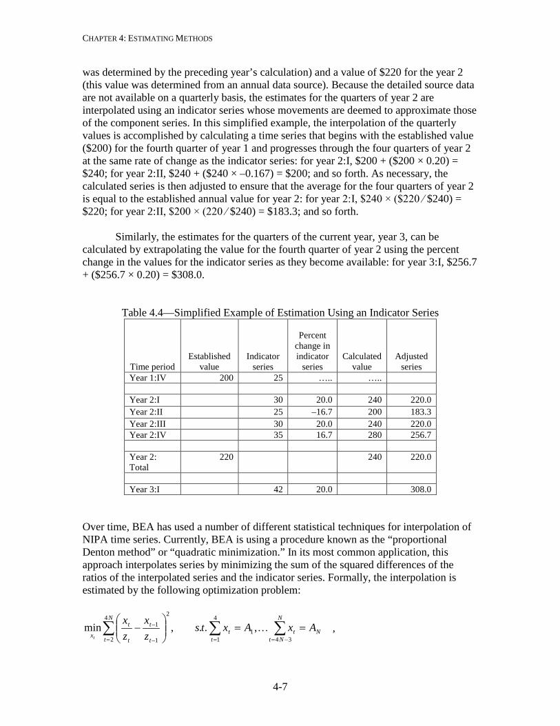
CHAPTER 4: ESTIMATING METHODS

4-7

was determined by the preceding year’s calculation) and a value of $220 for the year 2 (this value was determined from an annual data source). Because the detailed source data are not available on a quarterly basis, the estimates for the quarters of year 2 are interpolated using an indicator series whose movements are deemed to approximate those of the component series. In this simplified example, the interpolation of the quarterly values is accomplished by calculating a time series that begins with the established value ($200) for the fourth quarter of year 1 and progresses through the four quarters of year 2 at the same rate of change as the indicator series: for year 2:I, $200 + ($200 × 0.20) = $240; for year 2:II, $240 + ($240 × –0.167) = $200; and so forth. As necessary, the calculated series is then adjusted to ensure that the average for the four quarters of year 2 is equal to the established annual value for year 2: for year 2:I, $240 × ($220 ∕ $240) = $220; for year 2:II, $200 × (220 ∕ $240) = $183.3; and so forth.

Similarly, the estimates for the quarters of the current year, year 3, can be

calculated by extrapolating the value for the fourth quarter of year 2 using the percent change in the values for the indicator series as they become available: for year 3:I, $256.7 + ($256.7 × 0.20) = $308.0.

Table 4.4—Simplified Example of Estimation Using an Indicator Series

Time period Established

value

Indicator series

Percent change in indicator

series

Calculated value

Adjusted series

Year 1:IV 200 25 ….. ….. Year 2:I 30 20.0 240 220.0 Year 2:II 25 –16.7 200 183.3 Year 2:III 30 20.0 240 220.0 Year 2:IV 35 16.7 280 256.7 Year 2: Total

220 240 220.0

Year 3:I 42 20.0 308.0

Over time, BEA has used a number of different statistical techniques for interpolation of NIPA time series. Currently, BEA is using a procedure known as the “proportional Denton method” or “quadratic minimization.” In its most common application, this approach interpolates series by minimizing the sum of the squared differences of the ratios of the interpolated series and the indicator series. Formally, the interpolation is estimated by the following optimization problem:

,

∑∑∑−=== −

− ==

−

N

NtNt

tt

N

t t

t

t

t

xAxAxts

zx

zx

t 34

4

11

4

2

2

1

1 ,..,min

CHAPTER 4: ESTIMATING METHODS

4-8

where z is the indicator series, x is the interpolated series, A are the annual controls that the interpolated series must sum to, and N is the number of years for the interpolation. This example shows an annual-to-quarterly interpolation. The same method can also be used for annual-to-monthly and quarterly-to-monthly interpolation.3 Three special estimation methods In certain cases where primary source data are not available, one or more of the following special methods—commodity flow, retail control, or perpetual inventory—may be used to estimate values. Commodity-flow method

The commodity-flow method is generally used to derive estimates in economic census years for various components of consumer spending, equipment and software, and the commodity detail for state and local government consumption expenditures and gross investment. An abbreviated form of this method is used to prepare estimates of investment in equipment in nonbenchmark years, and an even more abbreviated form is used to prepare the current quarterly estimates of investment in equipment.

The commodity-flow method begins with estimates of the domestic output or domestic sales of a commodity valued in producers’ prices.4 Then, estimates of the domestic supply of that commodity—the amount that is available for domestic consumption—are prepared by adding imports and by subtracting exports and inventory change. Next, the domestic supply of the commodity is allocated among domestic purchasers—that is, persons, business, and government. Finally, the estimates are converted to purchasers’ prices.5 The commodity-flow method is illustrated in table 4.5. First, domestic shipments—the value of shipments of the commodity produced by domestic firms at producers’ prices—are converted to net supply, by adding imports and subtracting exports, government purchases, and change in inventories (a positive change in inventories reduces net supply and a negative change in inventories raises net supply) (in the example, $100 + $40 – $10 – $5 – $5 = $120). Portions of the net supply are then allocated among business intermediate purchases and consumer spending. This allocation may be based on relationships from the most recent economic census or on information from other sources (such as spending by consumers as determined by the retail control method). In this example, it is assumed that one-fourth of net supply is allocated to 3 See Baoline Chen and Stephen H. Andrews, “An Empirical Review of Methods for Temporal Distribution and Interpolation in the National Accounts,” Survey 88 (May 2008): 31–37. 4 Producers’ prices are the prices received by producers for the goods and services they sell. These prices include sales and excise taxes but exclude domestic transportation costs and trade margins. Trade margins, or markups, reflect the value added by wholesalers and retailers in the distribution of a commodity from producers to final purchasers. 5 Purchasers’ prices are the prices paid by intermediate and final purchasers for the goods and services they buy. These prices are equal to producers’ prices plus domestic transportation costs and trade margins.

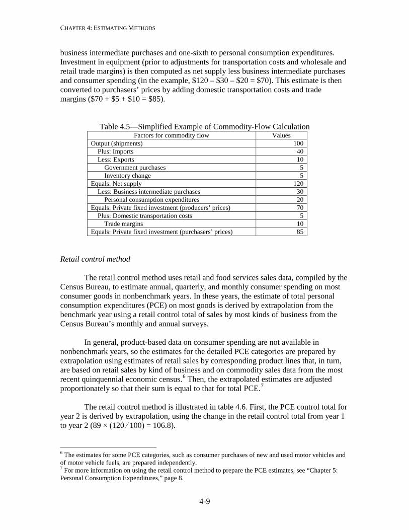
CHAPTER 4: ESTIMATING METHODS

4-9

business intermediate purchases and one-sixth to personal consumption expenditures. Investment in equipment (prior to adjustments for transportation costs and wholesale and retail trade margins) is then computed as net supply less business intermediate purchases and consumer spending (in the example, $120 – $30 – $20 = $70). This estimate is then converted to purchasers’ prices by adding domestic transportation costs and trade margins ($70 + $5 + $10 = $85).

Table 4.5—Simplified Example of Commodity-Flow Calculation Factors for commodity flow Values

Output (shipments) 100 Plus: Imports 40 Less: Exports 10 Government purchases 5 Inventory change 5 Equals: Net supply 120 Less: Business intermediate purchases 30 Personal consumption expenditures 20 Equals: Private fixed investment (producers’ prices) 70 Plus: Domestic transportation costs 5 Trade margins 10 Equals: Private fixed investment (purchasers’ prices) 85

Retail control method

The retail control method uses retail and food services sales data, compiled by the

Census Bureau, to estimate annual, quarterly, and monthly consumer spending on most consumer goods in nonbenchmark years. In these years, the estimate of total personal consumption expenditures (PCE) on most goods is derived by extrapolation from the benchmark year using a retail control total of sales by most kinds of business from the Census Bureau’s monthly and annual surveys.

In general, product-based data on consumer spending are not available in

nonbenchmark years, so the estimates for the detailed PCE categories are prepared by extrapolation using estimates of retail sales by corresponding product lines that, in turn, are based on retail sales by kind of business and on commodity sales data from the most recent quinquennial economic census.6 Then, the extrapolated estimates are adjusted proportionately so that their sum is equal to that for total PCE.7

The retail control method is illustrated in table 4.6. First, the PCE control total for

year 2 is derived by extrapolation, using the change in the retail control total from year 1 to year 2 (89 × (120 ∕ 100) = 106.8).

6 The estimates for some PCE categories, such as consumer purchases of new and used motor vehicles and of motor vehicle fuels, are prepared independently. 7 For more information on using the retail control method to prepare the PCE estimates, see “Chapter 5: Personal Consumption Expenditures,” page 8.

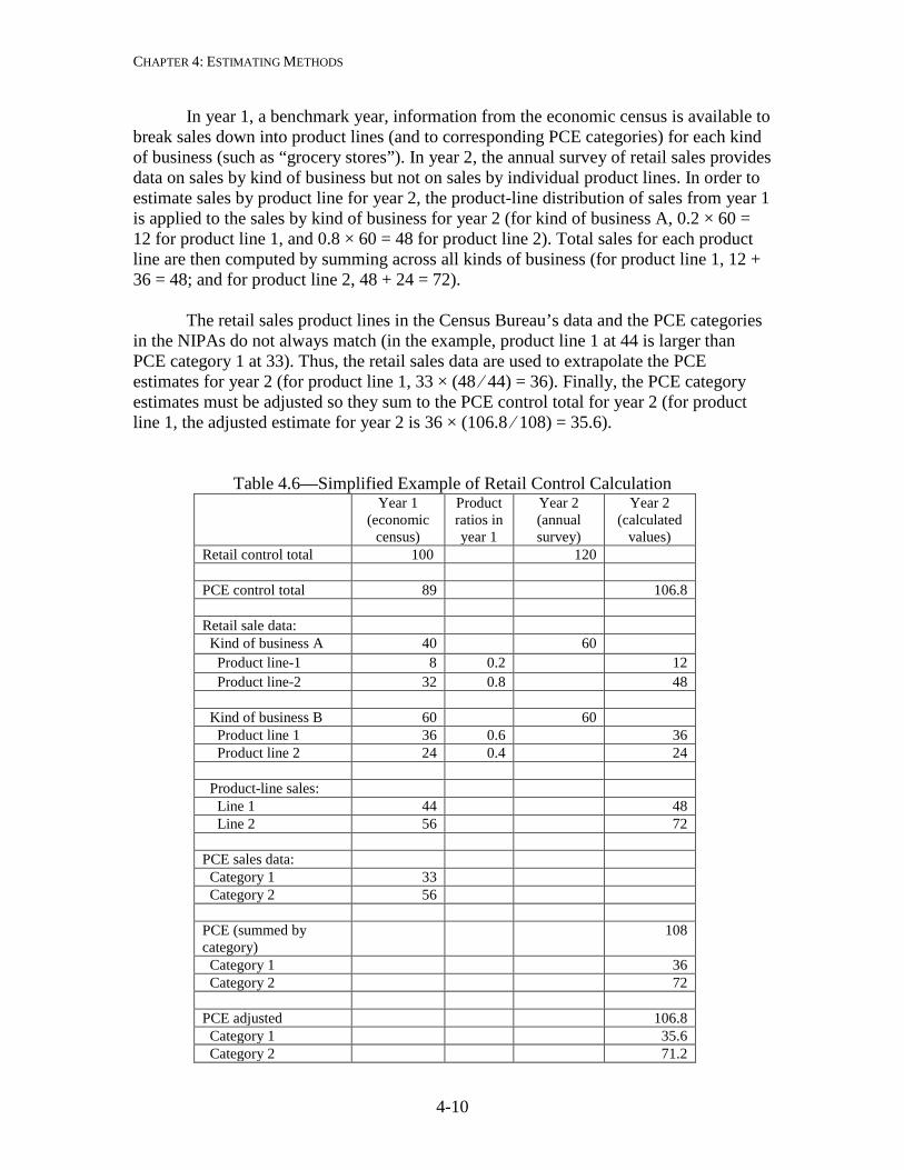
CHAPTER 4: ESTIMATING METHODS

4-10

In year 1, a benchmark year, information from the economic census is available to break sales down into product lines (and to corresponding PCE categories) for each kind of business (such as “grocery stores”). In year 2, the annual survey of retail sales provides data on sales by kind of business but not on sales by individual product lines. In order to estimate sales by product line for year 2, the product-line distribution of sales from year 1 is applied to the sales by kind of business for year 2 (for kind of business A, 0.2 × 60 = 12 for product line 1, and 0.8 × 60 = 48 for product line 2). Total sales for each product line are then computed by summing across all kinds of business (for product line 1, 12 + 36 = 48; and for product line 2, 48 + 24 = 72).

The retail sales product lines in the Census Bureau’s data and the PCE categories

in the NIPAs do not always match (in the example, product line 1 at 44 is larger than PCE category 1 at 33). Thus, the retail sales data are used to extrapolate the PCE estimates for year 2 (for product line 1, 33 × (48 ∕ 44) = 36). Finally, the PCE category estimates must be adjusted so they sum to the PCE control total for year 2 (for product line 1, the adjusted estimate for year 2 is 36 × (106.8 ∕ 108) = 35.6).

Table 4.6—Simplified Example of Retail Control Calculation

Year 1 (economic

census)

Product ratios in year 1

Year 2 (annual survey)

Year 2 (calculated

values) Retail control total 100 120 PCE control total 89 106.8 Retail sale data: Kind of business A 40 60 Product line-1 8 0.2 12 Product line-2 32 0.8 48 Kind of business B 60 60 Product line 1 36 0.6 36 Product line 2 24 0.4 24 Product-line sales: Line 1 44 48 Line 2 56 72 PCE sales data: Category 1 33 Category 2 56 PCE (summed by category)

108

Category 1 36 Category 2 72 PCE adjusted 106.8 Category 1 35.6 Category 2 71.2

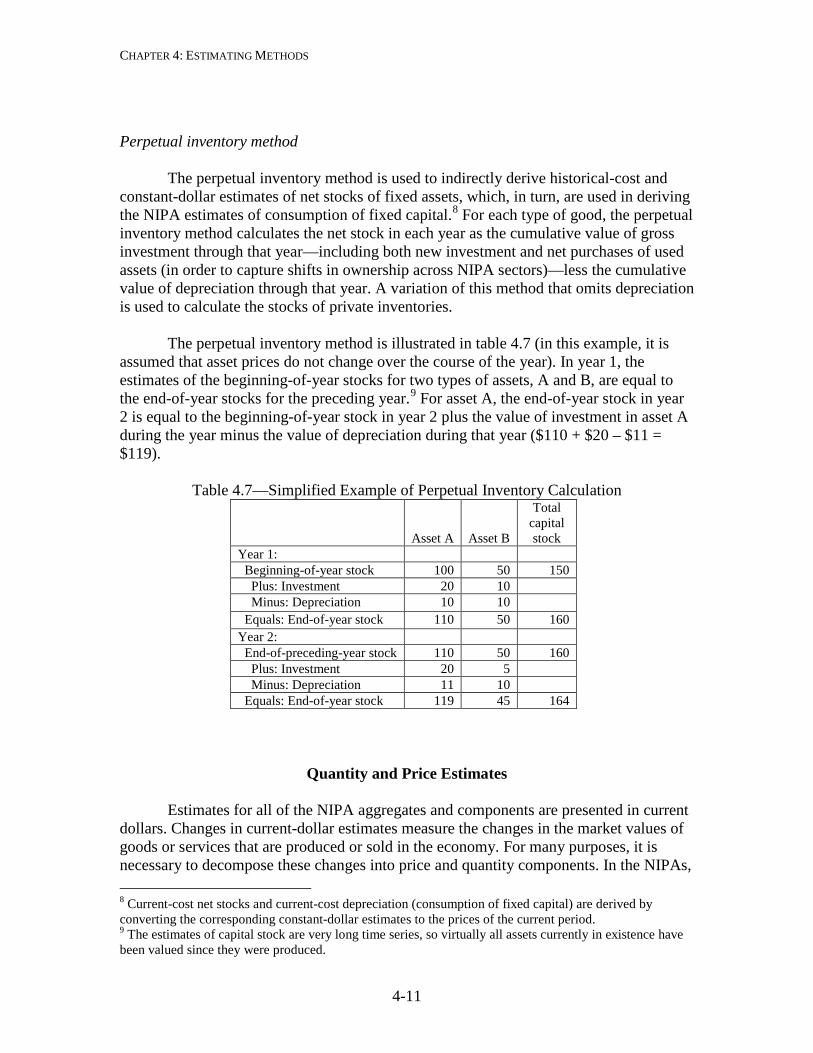
CHAPTER 4: ESTIMATING METHODS

4-11

Perpetual inventory method

The perpetual inventory method is used to indirectly derive historical-cost and constant-dollar estimates of net stocks of fixed assets, which, in turn, are used in deriving the NIPA estimates of consumption of fixed capital.8 For each type of good, the perpetual inventory method calculates the net stock in each year as the cumulative value of gross investment through that year—including both new investment and net purchases of used assets (in order to capture shifts in ownership across NIPA sectors)—less the cumulative value of depreciation through that year. A variation of this method that omits depreciation is used to calculate the stocks of private inventories. The perpetual inventory method is illustrated in table 4.7 (in this example, it is assumed that asset prices do not change over the course of the year). In year 1, the estimates of the beginning-of-year stocks for two types of assets, A and B, are equal to the end-of-year stocks for the preceding year.9 For asset A, the end-of-year stock in year 2 is equal to the beginning-of-year stock in year 2 plus the value of investment in asset A during the year minus the value of depreciation during that year ($110 + $20 – $11 = $119).

Table 4.7—Simplified Example of Perpetual Inventory Calculation

Asset A Asset B

Total capital stock

Year 1: Beginning-of-year stock 100 50 150 Plus: Investment 20 10 Minus: Depreciation 10 10 Equals: End-of-year stock 110 50 160 Year 2: End-of-preceding-year stock 110 50 160 Plus: Investment 20 5 Minus: Depreciation 11 10 Equals: End-of-year stock 119 45 164

Quantity and Price Estimates Estimates for all of the NIPA aggregates and components are presented in current dollars. Changes in current-dollar estimates measure the changes in the market values of goods or services that are produced or sold in the economy. For many purposes, it is necessary to decompose these changes into price and quantity components. In the NIPAs, 8 Current-cost net stocks and current-cost depreciation (consumption of fixed capital) are derived by converting the corresponding constant-dollar estimates to the prices of the current period. 9 The estimates of capital stock are very long time series, so virtually all assets currently in existence have been valued since they were produced.

CHAPTER 4: ESTIMATING METHODS

4-12

prices and quantities are expressed as index numbers with the reference year—at present, the year 2005—equal to 100. For selected series, quantities—or “real” (inflation adjusted) measures—are also expressed in chained (2005) dollars. (Period-to-period changes in quantities and prices are expressed as percent changes at annual rates; see “Statistical Tools and Conventions” in the appendix to this chapter.)

BEA prepares quantity estimates for GDP and its product-side components and

for a few other aggregates and components. (For an illustration of the calculation of these estimates from a set of quantity and price information, see “Calculation of Output and Price Indexes” in the appendix to this chapter.) Estimates for detailed components

For the detailed NIPA components, the quantity estimates are prepared using one of three methods—deflation, quantity extrapolation, or direct valuation—depending on the availability of source data. The quantity estimates are expressed as real values with 2005 (at present) as the reference year.

Deflation. Because the source data available for most components of GDP are

measured in dollars rather than in units, the quantities of most of the detailed components are obtained by deflation. For deflation, quantities are calculated by dividing the current-dollar value of the component by an “appropriate” price index (with the reference-year value set to 100).10

Qt = (ptqt)∕(pt∕po), where pt and qt are observed prices and quantities in the current year and po is the observed price in the reference year.

Thus, for example, if the current-dollar value for the component series is $14 in 2006 and the appropriate price index is 112 in 2006, then the quantity estimate for the component series in 2006 is ($14 ∕ (112 ∕ 100)), or $12.50.

Quantity extrapolation. The other two methods are similar in that they both are derived using quantity data. Quantity extrapolation is used when a quantity indicator series is available that approximates the movements of the component series. In this method, the quantity estimate is obtained by using the indicator series to extrapolate from the reference-year value. Qt = poqo+((poqo)×((qt′ –qo′)∕qo′)), where q′ represents the quantity indicator series. For example, if the dollar value of the component series is $10 in 2005 and the quantity indicator series shows an increase of 25 percent in 2006, then the quantity estimate for the component series in 2006 is ($10 + ($10 × 25/100)), or $12.50. 10 A price index is appropriate if its definition and coverage closely match those of the series being deflated.

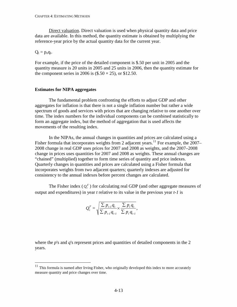
CHAPTER 4: ESTIMATING METHODS

4-13

Direct valuation. Direct valuation is used when physical quantity data and price data are available. In this method, the quantity estimate is obtained by multiplying the reference-year price by the actual quantity data for the current year. Qt = poqt. For example, if the price of the detailed component is $.50 per unit in 2005 and the quantity measure is 20 units in 2005 and 25 units in 2006, then the quantity estimate for the component series in 2006 is ($.50 × 25), or $12.50. Estimates for NIPA aggregates The fundamental problem confronting the efforts to adjust GDP and other aggregates for inflation is that there is not a single inflation number but rather a wide spectrum of goods and services with prices that are changing relative to one another over time. The index numbers for the individual components can be combined statistically to form an aggregate index, but the method of aggregation that is used affects the movements of the resulting index. In the NIPAs, the annual changes in quantities and prices are calculated using a Fisher formula that incorporates weights from 2 adjacent years.11 For example, the 2007–2008 change in real GDP uses prices for 2007 and 2008 as weights, and the 2007–2008 change in prices uses quantities for 2007 and 2008 as weights. These annual changes are “chained” (multiplied) together to form time series of quantity and price indexes. Quarterly changes in quantities and prices are calculated using a Fisher formula that incorporates weights from two adjacent quarters; quarterly indexes are adjusted for consistency to the annual indexes before percent changes are calculated. The Fisher index ( F

tQ ) for calculating real GDP (and other aggregate measures of output and expenditures) in year t relative to its value in the previous year t-1 is

where the p's and q's represent prices and quantities of detailed components in the 2 years.

11 This formula is named after Irving Fisher, who originally developed this index to more accurately measure quantity and price changes over time.

,qpqp

qpqp

=Q1-tt

tt

1-t1-t

t1-tFt ∑

∑×

∑∑

CHAPTER 4: ESTIMATING METHODS

4-14

Because the first term in the Fisher formula is a Laspeyres quantity index ( QLt ), or

and the second term is a Paasche quantity index ( P

tQ ), or

the Fisher formula can also be expressed for year t as the geometric mean of these indexes as follows:

The percent change in real GDP (and in other measures of output and expenditures) from year t-1 to year t is calculated as

1.0).Q100( Ft –

Similarly, price indexes are calculated using the Fisher formula

which is the geometric mean of a Laspeyres price index ( L

tP ) and a Paasche price index ( P

tP ), or

,qpqp=Q

1-t1-t

t1-tLt ∑

∑

,qpqp

=Q1-tt

ttPt ∑

∑

.QQ=Q Pt

Lt

Ft ×

,qpqp

qpqp

=Pt1-t

tt

1-t1-t

1-ttFt ∑

∑×

∑∑

PP=P Pt

Lt

Ft × .

CHAPTER 4: ESTIMATING METHODS

4-15

The chain-type quantity index value for period t is ,QI=I Ft

F1-t

Ft × and the chain-

type price index is calculated analogously. Chain-type real output and price indexes are presented with the reference year (b) equal to 100; that is, Ib = 100.

The current-dollar change from year t-1 to year t expressed in the form of a ratio is equal to the product of the changes in the Fisher price and quantity indexes:

The same formulas are used to calculate the quarterly (and for some components, monthly) chain-type indexes. All quarterly chain-type indexes for completed years that have been included in an annual or comprehensive revision are adjusted so that the quarterly indexes average to the corresponding annual index. When an additional year is completed between annual revisions, the annual index is computed as the average of the quarterly indexes, so no adjustment is required to make the quarterly and annual indexes consistent. For example, until the 2008 annual revision was released, the chain-type indexes for the year 2007 were computed as the average of the four quarterly indexes for 2007. Properties of chain-type measures The chain-type indexes based on the Fisher formula have several advantages over the fixed-weighted indexes that BEA used before 1996.12

• They produce percent changes in quantities and prices that are not affected by the choice of the reference period.

• They eliminate the substitution bias in measures of real GDP growth that are derived using fixed-weighted indexes. This bias tends to cause an understatement of growth for periods before the reference year and an overstatement of growth for periods after the reference year.

• They eliminate the distortions of growth in components and in industries that result from the fixed-weighted indexes.

• They eliminate the anomalies that arise from using recent-period weights to measure periods in the past when a far different set of prices prevailed. For

12 For information on BEA’s introduction of chain-type indexes as its featured measure of real output and prices, see J. Steven Landefeld and Robert P. Parker, “Preview of the Comprehensive Revision of the National Income and Product Accounts: BEA’s New Featured Measures of Output and Prices,” Survey 75 (July 1995): 31–38. See also J. Steven Landefeld and Robert P. Parker, “BEA’s Chain Indexes, Time Series, and Measures of Long-Term Economic Growth,” Survey 77 (May 1997): 58–68; and J. Steven Landefeld, Brent R. Moulton, and Cindy M. Vojtech, “Chained-Dollar Indexes: Issues, Tips on Their Use, and Upcoming Changes,” Survey 83 (November 2003): 8–16.

Ft

Ft

-1tt

tt

-1t-1t

t-1t

t-1t

tt

-1t-1t

-1tt

-1t-1t

tt QP=qpqp

qpqp

qpqp

qpqp

=qpqp

×∑∑

×∑∑

×∑∑

×∑∑

∑∑ .

CHAPTER 4: ESTIMATING METHODS

4-16

example, the prices of defense equipment in the 2000s are not appropriate for measuring the real changes in defense spending in the 1940s.

• They eliminate the inconvenience and confusion associated with BEA’s previous practice of updating weights and years—and thereby rewriting economic history—about every 5 years.

Despite the greater accuracy provided by the chain-type indexes, users of

macroeconomic statistics need more than index numbers and percent changes. The earlier fixed-weighted estimates were denominated in constant dollars, and the real levels for the components of GDP added up to total GDP. Because the system was additive, the shares of the real components reflected their relative importance in total GDP. Similarly, in decomposing total GDP growth by component, the change in constant-dollar values measured the component’s contribution to the change in the fixed-weighted aggregate. For GDP and most of its components, BEA prepares estimates in chained dollars as well as chain-type indexes (see the appendix to this chapter). However, because these chained-dollar measures are not based on a single set of weights, they are not additive and thus do not yield accurate measures of shares and contributions to growth.

For real GDP and its major components, BEA provides tables that present accurate estimates of contributions to growth rates that are based on chain-type quantity indexes rather than on the chained-dollar estimates (see the appendix). In addition, BEA provides measures of percentage shares that are based on current-dollar values. Because current-dollar values provide the weights for the chain-type indexes, shares calculated from these estimates rather than from the chained-dollar estimates should be used to indicate the relative importance of components

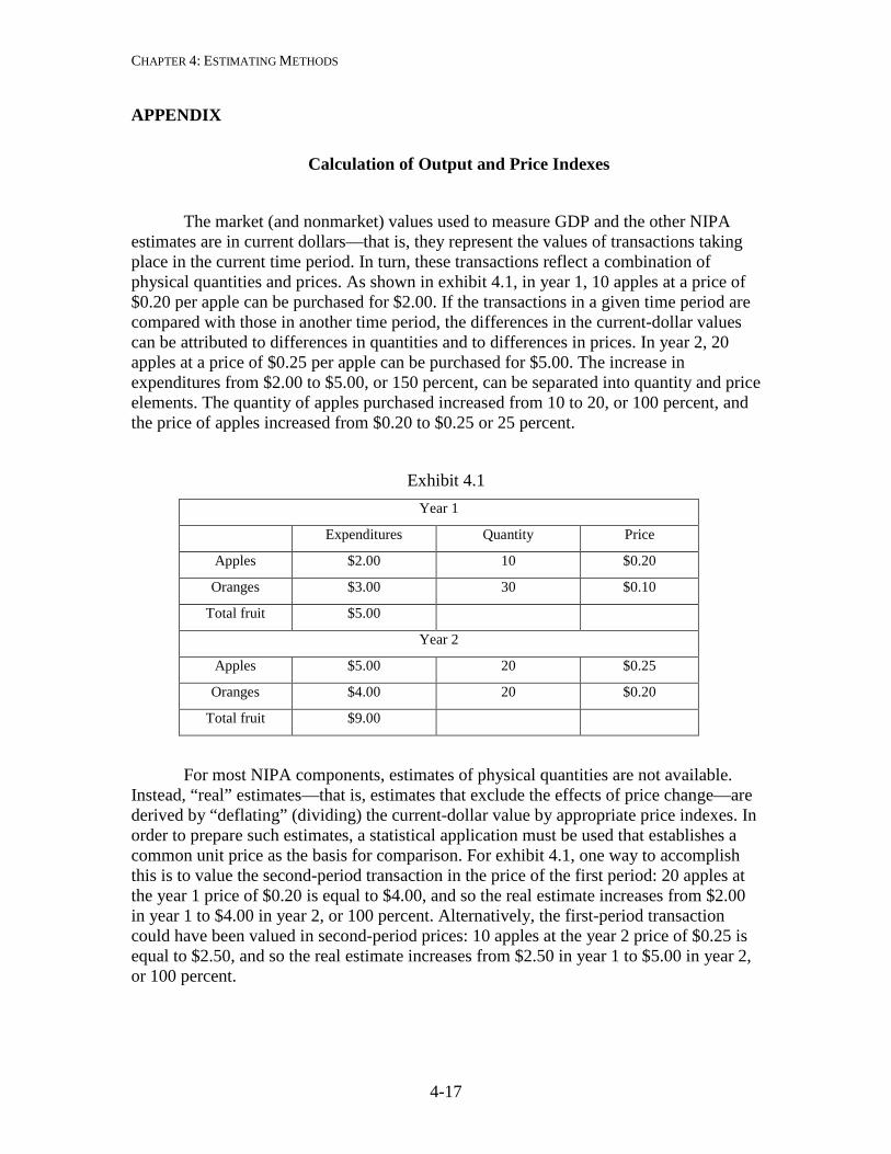
CHAPTER 4: ESTIMATING METHODS

4-17

APPENDIX

Calculation of Output and Price Indexes

The market (and nonmarket) values used to measure GDP and the other NIPA estimates are in current dollars—that is, they represent the values of transactions taking place in the current time period. In turn, these transactions reflect a combination of physical quantities and prices. As shown in exhibit 4.1, in year 1, 10 apples at a price of $0.20 per apple can be purchased for $2.00. If the transactions in a given time period are compared with those in another time period, the differences in the current-dollar values can be attributed to differences in quantities and to differences in prices. In year 2, 20 apples at a price of $0.25 per apple can be purchased for $5.00. The increase in expenditures from $2.00 to $5.00, or 150 percent, can be separated into quantity and price elements. The quantity of apples purchased increased from 10 to 20, or 100 percent, and the price of apples increased from $0.20 to $0.25 or 25 percent.

Exhibit 4.1 Year 1

Expenditures Quantity Price

Apples $2.00 10 $0.20

Oranges $3.00 30 $0.10

Total fruit $5.00

Year 2

Apples $5.00 20 $0.25

Oranges $4.00 20 $0.20

Total fruit $9.00

For most NIPA components, estimates of physical quantities are not available. Instead, “real” estimates—that is, estimates that exclude the effects of price change—are derived by “deflating” (dividing) the current-dollar value by appropriate price indexes. In order to prepare such estimates, a statistical application must be used that establishes a common unit price as the basis for comparison. For exhibit 4.1, one way to accomplish this is to value the second-period transaction in the price of the first period: 20 apples at the year 1 price of $0.20 is equal to $4.00, and so the real estimate increases from $2.00 in year 1 to $4.00 in year 2, or 100 percent. Alternatively, the first-period transaction could have been valued in second-period prices: 10 apples at the year 2 price of $0.25 is equal to $2.50, and so the real estimate increases from $2.50 in year 1 to $5.00 in year 2, or 100 percent.

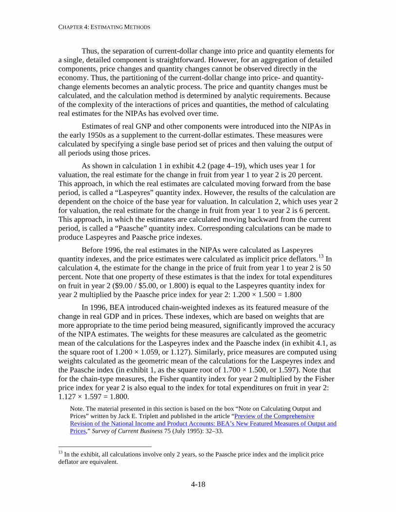
CHAPTER 4: ESTIMATING METHODS

4-18

Thus, the separation of current-dollar change into price and quantity elements for a single, detailed component is straightforward. However, for an aggregation of detailed components, price changes and quantity changes cannot be observed directly in the economy. Thus, the partitioning of the current-dollar change into price- and quantity-change elements becomes an analytic process. The price and quantity changes must be calculated, and the calculation method is determined by analytic requirements. Because of the complexity of the interactions of prices and quantities, the method of calculating real estimates for the NIPAs has evolved over time.

Estimates of real GNP and other components were introduced into the NIPAs in the early 1950s as a supplement to the current-dollar estimates. These measures were calculated by specifying a single base period set of prices and then valuing the output of all periods using those prices.

As shown in calculation 1 in exhibit 4.2 (page 4–19), which uses year 1 for valuation, the real estimate for the change in fruit from year 1 to year 2 is 20 percent. This approach, in which the real estimates are calculated moving forward from the base period, is called a “Laspeyres” quantity index. However, the results of the calculation are dependent on the choice of the base year for valuation. In calculation 2, which uses year 2 for valuation, the real estimate for the change in fruit from year 1 to year 2 is 6 percent. This approach, in which the estimates are calculated moving backward from the current period, is called a “Paasche” quantity index. Corresponding calculations can be made to produce Laspeyres and Paasche price indexes.

Before 1996, the real estimates in the NIPAs were calculated as Laspeyres quantity indexes, and the price estimates were calculated as implicit price deflators.13 In calculation 4, the estimate for the change in the price of fruit from year 1 to year 2 is 50 percent. Note that one property of these estimates is that the index for total expenditures on fruit in year 2 ($9.00 / $5.00, or 1.800) is equal to the Laspeyres quantity index for year 2 multiplied by the Paasche price index for year 2: 1.200 × 1.500 = 1.800

In 1996, BEA introduced chain-weighted indexes as its featured measure of the change in real GDP and in prices. These indexes, which are based on weights that are more appropriate to the time period being measured, significantly improved the accuracy of the NIPA estimates. The weights for these measures are calculated as the geometric mean of the calculations for the Laspeyres index and the Paasche index (in exhibit 4.1, as the square root of 1.200 × 1.059, or 1.127). Similarly, price measures are computed using weights calculated as the geometric mean of the calculations for the Laspeyres index and the Paasche index (in exhibit 1, as the square root of 1.700 × 1.500, or 1.597). Note that for the chain-type measures, the Fisher quantity index for year 2 multiplied by the Fisher price index for year 2 is also equal to the index for total expenditures on fruit in year 2: 1.127 × 1.597 = 1.800.

Note. The material presented in this section is based on the box “Note on Calculating Output and Prices” written by Jack E. Triplett and published in the article “Preview of the Comprehensive Revision of the National Income and Product Accounts: BEA’s New Featured Measures of Output and Prices,” Survey of Current Business 75 (July 1995): 32–33.

13 In the exhibit, all calculations involve only 2 years, so the Paasche price index and the implicit price deflator are equivalent.

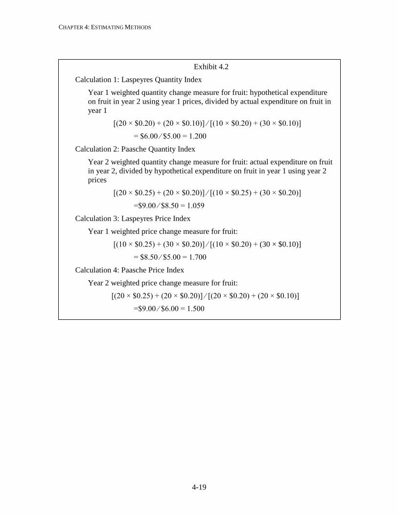
CHAPTER 4: ESTIMATING METHODS

4-19

Exhibit 4.2

Calculation 1: Laspeyres Quantity Index

Year 1 weighted quantity change measure for fruit: hypothetical expenditure on fruit in year 2 using year 1 prices, divided by actual expenditure on fruit in year 1

[(20 × $0.20) + (20 × $0.10)] ∕ [(10 × $0.20) + (30 × $0.10)]

= $6.00 ∕ $5.00 = 1.200

Calculation 2: Paasche Quantity Index

Year 2 weighted quantity change measure for fruit: actual expenditure on fruit in year 2, divided by hypothetical expenditure on fruit in year 1 using year 2 prices

[(20 × $0.25) + (20 × $0.20)] ∕ [(10 × $0.25) + (30 × $0.20)]

=$9.00 ∕ $8.50 = 1.059

Calculation 3: Laspeyres Price Index

Year 1 weighted price change measure for fruit:

[(10 × $0.25) + (30 × $0.20)] ∕ [(10 × $0.20) + (30 × $0.10)]

= $8.50 ∕ $5.00 = 1.700

Calculation 4: Paasche Price Index

Year 2 weighted price change measure for fruit:

[(20 × $0.25) + (20 × $0.20)] ∕ [(20 × $0.20) + (20 × $0.10)]

=$9.00 ∕ $6.00 = 1.500

CHAPTER 4: ESTIMATING METHODS

4-20

Statistical Tools and Conventions This section describes some of the statistical tools and conventions that BEA uses in preparing and presenting the NIPA estimates. In general, these statistical operations are used to transform the estimates into alternative formats that facilitate analytical or presentational uses. Chained-dollar measures

As a supplement to its chain-type quantity indexes, BEA prepares measures of real GDP and its components in a dollar-denominated form, designated “chained (2005) dollar” estimates. For GDP and most other series, the chained-dollar value CDF

t is calculated by multiplying the reference year current-dollar value qp bb∑ )by the chain-type Fisher quantity index ( I F

t ) and dividing by 100. For period t,

/100I Ftqp=CD Ft bb ×∑ .

Thus, for example, if a current-dollar GDP component is equal to $200 in 2005 and if the quantity index for this component increased 15 percent by 2008, then the chained (2005) dollar value of this component in 2008 would be $200 x 115 ∕ 100, or $230.

The chained (2005) dollar estimates provide measures to calculate the percent changes for GDP and its components that are consistent with those calculated from the chain-type quantity indexes; any differences are small and due to rounding. For most components of GDP, the chained-dollar estimates also provide rough approximations of their relative importance and of their contributions to real GDP growth for years close to 2005. However, for components—such as computers and other high-tech equipment—with rapid growth in real output and sharply falling prices, the chained-dollar levels (as distinct from chain-weighted indexes and percent changes) will overstate their relative importance to GDP growth.

In addition, chained-dollar values for the detailed GDP components will not

necessarily sum to the chained-dollar estimate of GDP (or of any intermediate aggregate), because the relative prices used as weights for any period other than the reference year differ from those used for the reference year. BEA provides a measure of the extent of such differences by showing a “residual” line on chained-dollar tables that indicates the difference between GDP (and other major aggregates) and the sum of the most detailed components in the table.

For periods close to the reference year, when there usually has not been much

change in the relative prices that are used as the weights for calculating the chain-type index, the residuals tend to be small, and the chained (2005) dollar estimates can be used to approximate the contributions to growth and to aggregate the detailed estimates.

CHAPTER 4: ESTIMATING METHODS

4-21

However, it is preferable to use estimates of exact contributions, which are described in the next section.

Some exceptions to the above methodology are made for a few components of

GDP. For cases in which the components of an aggregate include large negative values, the Fisher formula cannot be used because it would require taking the square root of a negative number. In such cases, one of two other methods is used.

• Quantity estimates are calculated as the sum of, or as the difference between, chained-dollar series that measure flows. For example, real net exports is derived as the difference between real exports and real imports.

• Quantity estimates are calculated as the difference between measures of chain-weighted stocks. For example, the real annual change in private inventories is derived as the difference between real beginning-of-year inventories and real end-of-year inventories.

The inability to calculate a particular Fisher quantity index (for example, for

change in private inventories) because of negative values usually does not extend to the calculation of higher level aggregates (for example, quantity indexes for gross private domestic investment and for GDP can be computed). The calculation of contributions to percent change is not affected by negative values, so they can be calculated for all components.

The chain-dollar estimates are used in the calculation of another price index, the

implicit price deflator (IPD). The IPDFt for period t is calculated as the ratio of the

current-dollar value to the corresponding chained-dollar value, multiplied by 100, as follows:

For all aggregates and components and for all time periods, the value of the IPD is very close to the value of the corresponding chain-type price index. Note that this definition of the IPD differs from that used before the introduction of chain-type measures in1996, when the IPD was defined as the ratio of the current-dollar value to the corresponding constant-dollar value.

Contributions to percent change

As one moves further away from the reference year, the residual tends to become

larger, and the chained-dollar estimates are less useful for analyses of contributions to growth. For this reason, BEA also shows contributions of major components to the percent change in real GDP (and to the percent change in other major aggregates) that use exact formulas for attributing growth.

100CD

qp=IPD F

t

ttFt ×

∑.

CHAPTER 4: ESTIMATING METHODS

4-22

The contributions to percent change in a real aggregate, such as real GDP, provide

a measure of the composition of growth in the aggregate that is not affected by the nonadditivity of its components. This property makes contributions to percent change a valuable tool for economic analysis. The contribution to percent change ( ∆ ti,C% ) in an aggregate in period t that is attributable to the quantity change in component i is defined by the formula where

PFt is the Fisher price index for the aggregate in period t relative to period t-1;

pi,t is the price of the component i in period t; and qi,t is the quantity of the component i in period t.

The summation with subscript j in the denominator includes all the deflation-level components of the aggregate. Contributions of subaggregates (such as PCE goods) to the percent change of the aggregate (say, PCE or GDP) are calculated by summing the contributions of all the deflation-level components contained in the subaggregate.14

For annual estimates, no adjustments are required for the contributions to sum exactly to the percent change in the aggregate. For quarterly estimates, adjustments are required to offset the effects of adjustments that were made to equate the average of the quarterly estimates to the corresponding annual estimate and to express the percent change at annual rate. The same formula is used for both annual and quarterly estimates of contributions to percent change in all periods. The only variation in the method of calculation is that the annual contributions for the most recent year are based on a weighted average of the quarterly contributions until the next annual revision. Annual rates Quarterly and monthly NIPA estimates in current and chained dollars are presented at annual rates, which show the value that would be registered if the level of activity measured for a quarter or for a month were maintained for a full year. Annual rates are used so that periods of different lengths—for example, quarters and years—may be easily compared. These annual rates are determined simply by multiplying the estimated rate of activity by 4 (for quarterly data) or by 12 (for monthly data).

14 See Marshall B. Reinsdorf, W. Erwin Diewert, and Christian Ehemann, “Additive Decompositions for Fisher, Tornqvist, and Geometric Mean Indexes,” Journal of Economic and Social Measurement 28 (2002): 51–61, www.econ.ubc.ca/diewert/additive.pdf.

,))/((

)())/((100%

1,1,,

1,,1,,, ∑ −−

−−

×+−×+

×=∆j tjtj

Fttj

tititiF

ttiti qpPp

qqpPpC

CHAPTER 4: ESTIMATING METHODS

4-23

Growth rates

Percent changes in the estimates are also expressed at annual rates, which show the value that would be registered if the pace of activity measured for a quarter or for a month were maintained for a full year. Calculating these changes requires a variant of the compound interest formula,

where

r is the percent change at an annual rate; GDPt is the level of activity in the later period; GDP0 is the level of activity in the earlier period; m is the periodicity of the data (for example, 1 for annual data, 4 for quarterly, or 12 for monthly); and n is the number of periods between the earlier and later periods (that is, t-0). Thus, for example, if a component increases from $100 in the first quarter to $105 in the second quarter (5 percent at a quarterly rate), the annual rate of increase is (($105/$100)4/1 – 1) x 100 = 21.6 percent. Rebasing an index In the NIPAs, quantities and prices are generally expressed as index numbers with a reference year—at present, the year 2005—equal to 100. These indexes can easily be rebased to a different reference year without changing the relationship between the series values. To rebase, divide the entire index by the index value of the desired reference year. As illustrated in table 4.8, the original index is rebased from year 1 to year 2 by dividing each of the original index values by the index value in year 2 (for year 1, 100.0 ∕ 110.0 = 90.9). Note that the year-to-year percent changes are unaffected by the rebasing.

Table 4.8—Example of Index Rebasing

Year Original

index

Percent change

Rebased index

Percent change

1 100.0 ….. 90.9 ….. 2 110.0 10.0 100.0 10.0 3 120.0 9.1 109.1 9.1 4 130.0 8.3 118.2 8.3

100,1GDPGDP=r

0

tm/n

×

–