concepts and methods of the u.s. national income and product accounts · · 2011-06-14the u.s....
TRANSCRIPT
Concepts and Methods of the U.S. National Income and Product Accounts
(Chapters 1–7)
November 2010
Preface The “NIPA Handbook” begins with introductory chapters that describe the fundamental concepts, definitions, classifications, and accounting framework that underlie the national income and product accounts (NIPAs) of the United States and the general sources and methods that are used to prepare the NIPA estimates. It continues with separate chapters that describe the sources and methods that are used to prepare the expenditure and income components of the accounts. The Handbook is intended to be a living reference that can be updated to reflect changes in concepts or methodology as they are introduced into the NIPAs. This release of the NIPA Handbook consists of updated versions of the first five chapters to reflect the 2010 annual revision and of new chapters on private fixed investment and on change in private inventories. Additional chapters will be incorporated as they become available.
Acknowledgments
Douglas R. Fox, formerly of the Bureau of Economic Analysis (BEA), is leading the preparation of this Handbook. Major contributors include Stephanie H. McCulla, Eugene P. Seskin, and Shelly Smith, all of BEA’s National Income and Wealth Division (NIWD). Technical expertise has been provided by NIWD staff—including Jeffrey W. Crawford, Clinton P. McCully, and Jennifer A. Ribarsky. Brent R. Moulton, BEA’s Associate Director for National Economic Accounts, and Carol E. Moylan, Chief of NIWD, have provided overall guidance.
Table of Contents CHAPTER 1: INTRODUCTION
The U.S. national income and product accounts (NIPAs) are a set of economic accounts that provide the framework for presenting detailed measures of U.S. output and income. This chapter introduces the NIPAs by answering several basic questions about their nature and purpose.
CHAPTER 2: FUNDAMENTAL CONCEPTS
The NIPAs are based on a consistent set of concepts and definitions. This chapter establishes the type and scope of the economic activities that are covered by the NIPA measures, and it describes several of the principal NIPA measures of these activities. It then discusses the classifications used in presenting the NIPA estimates, and it describes the accounting framework that underlies the NIPAs.
CHAPTER 3: PRINCIPAL SOURCE DATA
The NIPAs incorporate a vast amount of data from a variety of public and private sources. This chapter describes the principal source data that are used to prepare the current quarterly NIPA estimates, to prepare the annual revisions of the NIPAs, and to prepare the quinquennial comprehensive revisions of the NIPAs.
CHAPTER 4: ESTIMATING METHODS
Estimating methods are the steps that are taken to transform source data into estimates that are consistent with the concepts, definitions, and framework of the NIPAs. This chapter briefly describes some of the general methods that are used to prepare the current-dollar, quantity, and price estimates for the NIPAs. An appendix describes some of the statistical tools and conventions that are used in preparing and presenting the NIPA estimates.
CHAPTER 5: PERSONAL CONSUMPTION EXPENDITURES
Personal consumption expenditures (PCE) is the NIPA measure of consumer purchases of goods and services in the U.S. economy. This chapter describes the concepts, source data, and methods that underlie the PCE estimates. A technical note provides additional detail on the methodology for a number of key PCE components.
CHAPTER 6: PRIVATE FIXED INVESMENT
Private fixed investment (PFI) is the NIPA measure of spending by private business, nonprofit institutions, and households on fixed assets in the U.S. economy. This chapter describes the concepts, source data, and methods that underlie the PFI estimates. A technical note provides additional detail on the methodology for several key PFI components.
CHAPTER 7: CHANGE IN PRIVATE INVENTORIES
Change in private inventories (CIPI) is the NIPA measure of the value of the change in the physical volume of inventories owned by private businesses in the U.S. economy. This chapter describes the concepts, source data, and methods that underlie the CIPI estimates. Appendixes at the end of the chapter illustrate the relationship between business and NIPA inventory accounting and the basic steps used in the NIPA inventory calculations.
Additional chapters (forthcoming) Glossary (forthcoming) Selected References (forthcoming)
CHAPTER 1: INTRODUCTION What are the NIPAs? How did the NIPAs originate? How are the NIPA estimates used? How useful are the NIPA estimates?
How are the NIPA estimates prepared? Why are the NIPA estimates revised? Where are the NIPA estimates available? What are the NIPAs?
The NIPAs are one of the three major elements of the U.S. national economic accounts. The NIPAs display the value and composition of national output and the distribution of incomes generated in its production. (For information on the concepts and definitions underlying the NIPAs, see “Chapter 2: Fundamental Concepts.”)
The other major elements of the U.S. national economic accounts are the industry
accounts, which are also prepared by the Bureau of Economic Analysis (BEA), and the flow of funds accounts, which are prepared by the Federal Reserve Board. The industry accounts consist of the input-output (I-O) accounts, which trace the flow of goods and services among industries in the production process and which show the value added by each industry and the detailed commodity composition of national output, and the gross domestic product (GDP) by industry accounts, which measure the contribution of each private industry and of government to GDP.1 The flow of funds accounts record the acquisition of nonfinancial and financial assets (and the incurrence of liabilities) throughout the U.S. economy, the sources of the funds used to acquire those assets, and the value of assets held and of liabilities owed.2
In addition, BEA prepares two other sets of U.S. economic accounts: the
international accounts, which consist of the international transactions (balance of payments) accounts and the international investment position accounts; and the regional accounts, which consist of the estimates of GDP by state and by metropolitan area, of state personal income, and of local area personal income. Finally, the U.S. Bureau of Labor Statistics prepares estimates of productivity for the U.S. economy (which are partly
1 See U.S. Bureau of Economic Analysis, Concepts and Methods of the U.S. Input-Output Accounts (September 2006) at http://www.bea.gov/methodologies/index.htm; and see Brian C. Moyer, Mark A. Planting, Mahnaz Fahim Nader, and Sherlene K.S. Lum, “Preview of the Comprehensive Revision of the Annual Industry Accounts: Integrating the Annual Input-Output Accounts and Gross-Domestic-Product-by-Industry Accounts,” Survey of Current Business 84 (March 2004): 38–51. 2 See U.S. Board of Governors of the Federal Reserve System, Guide to the Flow of Funds Accounts (Board of Governors, Washington, DC, 2006); and see Albert M. Teplin, “The U.S. Flow of Funds Accounts and Their Uses,” Federal Reserve Bulletin (July 2001): 431–441.
1-1
CONCEPTS AND METHODS OF THE U.S. NATIONAL INCOME AND PRODUCT ACCOUNTS
based on the estimates of GDP). Altogether, the system of U.S. economic accounts presents a coherent, comprehensive, and consistent picture of U.S. economic activity.
The NIPAs provide information to help answer three basic questions. First, what is the output of the economy—its size, its composition, and its use? Second, what are the sources and uses of national income? Third, what are the sources of saving, which provides for investment in future production? The NIPA estimates are presented in a set of integrated accounts that show U.S. production, income, consumption, investment, and saving. The conceptual framework of the accounts is illustrated by seven summary accounts, and detailed estimates are provided in approximately 300 supporting NIPA tables. The NIPA information is supplemented by a set of fixed-asset accounts, which show the U.S. stock of fixed assets and consumer durable goods.3
The NIPAs feature some of the most closely watched economic statistics that influence the decisions made by government officials, business persons, and households. Foremost among these estimates is GDP, the most widely recognized measure of the nation’s production. In particular, the quarterly estimates of inflation-adjusted GDP provide the most comprehensive picture of current economic conditions in the United States. Other key NIPA estimates include the monthly estimates of personal income and outlays, which provide current information on consumer income, spending, and saving, and the quarterly estimates of corporate profits, which provide an economic measure of U.S. corporate financial performance. How did the NIPAs originate?
The NIPAs trace their origin back to the 1930s, when the lack of comprehensive economic data hampered efforts to develop policies to combat the Great Depression. In response to this need, the U.S. Department of Commerce commissioned future Nobel Laureate Simon Kuznets to develop estimates of national income. He coordinated the work of a group of researchers at the National Bureau of Economic Research and of his staff at the Commerce Department, and initial estimates were presented in a 1934 report to the U.S. Senate, National Income, 1929–32.
As the United States transitioned to a wartime economy in the early 1940s, it became apparent that planning for the war effort required a measure of national production. Annual estimates of “gross national expenditure,” which gradually evolved to gross national product (GNP), were introduced early in 1942 to complement the estimates of national income.4 The U.S. national income and product statistics were first presented as part of a complete and consistent double-entry accounting system in the summer of 1947. The accounts presented a framework for classifying and recording the economic transactions among major sectors: households, businesses, government, and international
3 See U.S. Bureau of Economic Analysis, Fixed Assets and Consumer Durable Goods in the United States, 1925–97 (September 2003) at http://www.bea.gov/methodologies/index.htm. 4 Until 1991, GNP was the featured measure of U.S. production. For an explanation of the difference between GNP and GDP, see the section “Geographic coverage” in chapter 2.
1-2
CONCEPTS AND METHODS OF THE U.S. NATIONAL INCOME AND PRODUCT ACCOUNTS
(termed “rest of the world”). This framework placed the GNP statistics in the broader context of the economy as a whole and provided a more complete picture of how the economy works.5
Since then, the national accounts have continued to expand in response to
demands for better and more detailed information on the U.S. economy. At the end of 1999, the Commerce Department named the invention and ongoing development of the NIPAs and its marquee measure GDP as “its greatest achievement of the century.”6 How are the NIPA estimates used?
The NIPAs provide government policymakers, business decision-makers, academics and other researchers, and the general public with information that enables them to follow and understand the performance of the U.S. economy. The following are among the principal uses of the NIPA estimates.
• Since their inception in the 1930s and 1940s, the NIPAs have become the mainstay of modern macroeconomic analysis. They provide comprehensive and consistent time series that can be used for measuring the long-term path of the U.S. economy, for analyzing trends and identifying factors in economic growth and productivity, and for tracking cyclical fluctuations in economic activity.
• The NIPAs provide the basis for macroeconomic forecasting models. These
mathematical models are developed using historical NIPA estimates and other variables with the aim of predicting short-term economic activity or long-term economic trends.
• Key NIPA estimates serve as primary indicators of the current condition of the
U.S. economy. In particular, the releases of the quarterly estimates of GDP and its components, of the quarterly estimates of corporate profits, and of the monthly estimates of personal income and personal consumption expenditures are closely anticipated and followed by Wall Street investors and analysts, the news media, and the general public.
• The NIPA estimates provide critical inputs to the formulation and execution of
macroeconomic policy and to the assessment of the effects of these policies. They are used by the White House and by Congress in formulating fiscal policy and by the Federal Reserve Board in formulating monetary policy.
• The NIPA estimates are used by the White House and Congress in preparing the
federal budget and tax projections. 5 See Rosemary D. Marcuss and Richard E. Kane, “U.S. National Income and Product Statistics: Born of the Great Depression and World War II,” Survey 87 (February 2007): 32–46. 6 “GDP: One of the Great Inventions of the 20th Century,” Survey 80 (January 2000): 6–14.
1-3
CONCEPTS AND METHODS OF THE U.S. NATIONAL INCOME AND PRODUCT ACCOUNTS
• The NIPA estimates are used in comparisons of the U.S. economy with the economies of other nations. Comparable international statistics facilitate assessments of relative economic performance among nations, and they provide the basis for tracking and analyzing the global economy.
• Detailed NIPA estimates can be used in examining interrelationships between
various sectors of the economy. For example, estimates of benefits paid under government assistance programs track flows of transfer payments from governments to households.
• The NIPA estimates are used by businesses and individuals in planning financial
and investment strategies. Such planning heavily depends on the near- and long-term prospects for economic growth.
• The NIPAs are an important data source for the other national economic accounts
and other economic statistics. For example, the NIPA estimates of owner-occupied housing, of motor vehicle output, and of bank-service charges are among the primary source data used in preparing the I-O accounts. In addition, the NIPA estimates are used in various analytical measures; for example, business-sector output is used as the numerator in the Bureau of Labor Statistics’ estimates of productivity for the U.S. economy.
• The NIPA framework provides the basis for developing analytical tools such as
satellite accounts, which are supplementary accounts that focus on the activities of a specific sector or segment of the economy. For example, the NIPAs provide the structural and statistical basis for the research and development satellite accounts.7
How useful are the NIPA estimates? The usefulness of the NIPA estimates is determined by how effective they are in meeting the above needs. This effectiveness may be summarized in terms of four characteristics: accuracy, reliability, relevancy, and integrity. Accuracy. Accuracy may be described in terms of how close the estimates come to measuring the concepts they are designed to measure. In the case of GDP, the estimate is accurate when it captures all production for final use but does not include production for intermediate use. In order to keep pace with innovations in the economy, such as the development of new online services, BEA must periodically review and update the definitions and methodologies of the NIPA aggregates and components to ensure that they represent complete and consistent estimates.
7 See Carol A. Robbins and Carol E. Moylan, “Research and Development Satellite Account Update,” Survey 87 (October 2007): 49–92.
1-4
CONCEPTS AND METHODS OF THE U.S. NATIONAL INCOME AND PRODUCT ACCOUNTS
Reliability. Reliability refers to the size and frequency of revisions to the NIPA estimates. An important indicator of reliability is the effectiveness of the initial estimates of GDP in providing a useful picture of U.S. economic activity. The results of periodic studies have confirmed that the initial estimates provide a reliable indication of whether economic growth is positive or negative, whether growth is accelerating or decelerating, whether growth is high or low relative to trend, and where the economy is in relation to the business cycle.8
Relevancy. Relevancy has two dimensions. First, relevancy refers to the length of
time before the estimates become available. Estimates that are not available soon enough for the intended use are not relevant. However, there is an implicit tradeoff between timeliness and accuracy, so BEA has developed a release cycle for the estimates that addresses this tradeoff (see the section “Why are the NIPA estimates revised?”).
Second, relevancy refers to the ability of the accounts to provide summary and
detailed estimates in analytical frameworks that help answer the questions being asked about the economy. Issues of relevance change as the economy changes, as policy concerns evolve, and as economic theory advances. For example, the increased integration of the world’s monetary, fiscal, and trade policies led to a growing need for the international comparability of economic statistics. Accordingly, the System of National Accounts (SNA) was developed by the international community in order to facilitate international comparisons of national economic statistics and to serve as a guide for countries as they develop their own economic statistics. BEA actively participated in preparing the 1993 revision of the SNA. Since 1993, BEA has incorporated many improvements to the NIPAs and its other economic accounts that have resulted in increased consistency with major SNA guidelines on GDP, investment, and saving.9
The following are examples of some of the major changes that have been introduced into the NIPAs to keep them relevant.
• In the 1950s, BEA developed and began to publish inflation-adjusted, or “real,” measures of output.
• In the 1980s, BEA significantly expanded its coverage of international trade in services in response to the proliferation in the volume and types of these global transactions.
• In the 1990s, BEA introduced more accurate measures of real output and of prices, developed estimates of investments in computer software, instituted the treatment of government purchases of structures and equipment as investment, and incorporated improved measures of high-tech products.
• In the early 2000s, BEA introduced improved measures of insurance and banking services, a new treatment of government as a producer of goods and services, and a substantially improved format for presenting the NIPAs.
8 For more information, see Dennis J. Fixler and Bruce T. Grimm, “The Reliability of the GDP and GDI Estimates,” Survey (February 2008): 16–32. 9 For more information, see Charles Ian Mead, Karin E. Moses, and Brent R. Moulton, “The NIPAs and the System of National Accounts,” Survey (December 2004): 17–32. For the latest edition of the SNA, see http://unstats.un.org/unsd/nationalaccount/SNA2008.pdf.
1-5

CONCEPTS AND METHODS OF THE U.S. NATIONAL INCOME AND PRODUCT ACCOUNTS
Integrity. One critical factor underlying the usefulness of the accounts is the trust
on the part of users that the NIPA estimates represent a truthful picture of the economy. That is, the preparation and release of the estimates must reflect the best methods and technical judgments available, free from any political or other inappropriate influence.
In recognition of the importance of its statistics and the trust placed in their
integrity, BEA strives to make its processes open and transparent and its releases objective and timely. For example, the NIPA estimates that are designated as “principal economic indicators”—GDP, personal income and outlays, and corporate profits—are prepared in accordance with Statistical Policy Directive Number 3 of the Office of Management and Budget, which provides standards for data collection, estimation, and evaluation and for the timely and orderly release of these sensitive economic statistics. BEA employs such standards in the preparation of all of its estimates.
As Alan Greenspan, former Chair of the Federal Reserve Board, stated about the national economic accounts, and specifically the estimates of GDP:
Though these estimates have a profound influence on markets when published and are the basis for federal budget projections and political rhetoric, I do not recall a single instance when the integrity of the estimates was called into question by informed observers. This is so despite the fact that, for many of the published preliminary figures, judgmental estimates for data not yet available are made, many of which affect the message of the accounts. It is a testament to the professionalism of the analysts that these judgments are never assumed to be driven by political imperatives. This cannot be said of statistical operations of all countries, and I think it is fair to say that the consequent ability of people to make decisions with greater confidence in the information at their disposal has contributed, in at least a small way, to our nation’s favorable economic performance.10
How are the NIPA estimates prepared?
The NIPA estimates are prepared by the staff of the Directorate for National Economic Accounts within the Bureau of Economic Analysis, an agency of the U.S. Department of Commerce. The process starts with identifying and obtaining source data that are appropriate as the basis for the estimates. These data largely originate from public sources, such as government surveys and administrative data, and they are supplemented by data from private sources, such as data from trade associations. (For more information, see “Chapter 3: Principal Source Data.”)
Ideally, the source data for each detailed component of the NIPAs would
correspond exactly to the concepts and structure of the accounts. Additionally, these data would be accurate, would have the needed coverage, would have the appropriate time of 10 “GDP: One of the Great Inventions of the 20th Century,” 13.
1-6
CONCEPTS AND METHODS OF THE U.S. NATIONAL INCOME AND PRODUCT ACCOUNTS
recording and valuation, and would be available quickly. In practice, the source data will never meet all of these criteria. Thus, BEA must develop estimating methods that adjust the data to the required concepts and that fill gaps in coverage and timing. (For more information, see “Chapter 4: Estimating Methods.”) Why are the NIPA estimates revised?
BEA revises the NIPA estimates for two related reasons. First, as noted earlier, the NIPAs serve a multitude of purposes, some of which require frequent and immediately available estimates and others of which require consistent, long-term time series. Second, much of the source data that BEA uses to prepare the estimates are part of statistical programs that provide, over time, more complete or otherwise better coverage—for example, monthly surveys that are superseded by an annual survey that is drawn from a larger sample or that collects more detailed information. To address this implicit tradeoff between estimates that are the most timely possible and estimates that are the most accurate possible, BEA has developed a release cycle for the NIPA estimates. This cycle progresses from current quarterly estimates, which are released soon after the end of the quarter and which are based on limited source data, to comprehensive-revision estimates, which are released about every 5 years and which incorporate the most extensive source data available.
For GDP and most other NIPA series, the set of three current quarterly estimates are released on the following schedule.11 “Advance” estimates are released near the end of the first month after the end of the quarter. Most of these estimates are based on initial data from monthly surveys; where source data are not yet available, the estimates are generally based on previous trends and judgment. “Second” and “third” quarterly estimates are released near the end of the second and third months, respectively; these estimates incorporate new and revised data from the monthly surveys and other monthly and quarterly source data that have subsequently become available. The current quarterly estimates provide the first look at the path of U.S. economic activity.
Annual revisions of the NIPAs are usually carried out each summer and cover the 3 previous calendar years. These estimates incorporate source data that are based on more extensive annual surveys, on annual data from other sources, and on later revisions to the monthly and quarterly source data.12 These revised NIPA estimates improve the quality
11 In the 2009 comprehensive revision of the NIPAs, BEA introduced new names for the second two vintages of the current quarterly estimates. Formerly, the “second” estimate was known as the “preliminary” estimate, and the “third” estimate” was known as the “final” estimate. The initial estimate continues to be named the “advance” estimate. (See Eugene P. Seskin and Shelly Smith, “Preview of the 2009 Comprehensive Revision of the NIPAs: Changes in Definitions and Presentations,” Survey 89 (March 2009): 19–20.) 12 Starting in 2010, BEA is adopting a flexible approach to annual revisions that allows improvements in concepts, definitions, and source data to be introduced and that allows the expansion of the 3-year revision period to earlier periods if necessary; see “BEA Briefing: Improving BEA’s Accounts Through Flexible Annual Revisions,” Survey 88 (June 2008): 29–32.
1-7
CONCEPTS AND METHODS OF THE U.S. NATIONAL INCOME AND PRODUCT ACCOUNTS
1-8
of the picture of U.S. economic activity, though the overall picture is generally similar to that shown by the current quarterly estimates.
Comprehensive revisions are carried out at about 5-year intervals and may result in revisions that extend back for many years.13 These estimates incorporate all of the best available source data, such as data from the quinquennial U.S. Economic Census. Comprehensive revisions also provide the opportunity to make definitional, statistical, and presentational changes that improve and modernize the accounts to keep pace with the ever-changing U.S. economy. Thus, these NIPA estimates represent the most accurate and relevant picture of U.S. economic activity. Where are the NIPA estimates available? All of the NIPA information is provided and updated on BEA’s website at www.bea.gov. The estimates are available in an interactive environment that enables users to view and download specified tables for selected time spans and in a variety of formats. The website also has descriptions of methodologies, articles and working papers, and release schedules.
The current quarterly estimates are first available in news releases that are posted on BEA’s website in accordance with a previously published schedule. These releases contain a brief description of the estimates and summary data tables. Shortly thereafter, the website presentation of the entire set of NIPA tables is updated to reflect the newly released estimates.
The NIPA estimates are also published in BEA’s monthly journal, Survey of
Current Business. The current estimates are presented each month in the article “GDP and the Economy” and in a set of selected NIPA tables. The annual revision is described in an article in the August issue, along with most of the full set of NIPA tables. Articles that explain upcoming changes in definitions, methodologies, and presentation—such as those made in connection with the comprehensive revision—and articles on other topics related to the NIPAs are published periodically.
13 The following is a list of the 13 NIPA comprehensive revisions to date: July 1947, July 1951, July 1954, July 1958, August 1965, January 1976, December 1980, December 1985, December 1991, January 1996, October 1999, December 2003, and July 2009.
CHAPTER 2: FUNDAMENTAL CONCEPTS Scope of the Estimates Production boundary Asset boundary Market and nonmarket output Geographic coverage Income and saving GDP and Other Major NIPA Measures Three ways to measure GDP Major NIPA aggregates Principal quantity and price measures Classification Sector Type of product Function Industry Legal form of organization Accounting Framework Accounting principles Conceptual derivation of the NIPAs The summary NIPAs
Scope of the Estimates Production boundary
One of the fundamental questions that must be addressed in preparing the national
economic accounts is how to define the production boundary—that is, what parts of the myriad human activities are to be included in or excluded from the measure of the economy’s production. According to the international System of National Accounts (SNA), “Economic production may be defined as an activity carried out under the control and responsibility of an institutional unit that uses inputs of labour, capital, and goods and services to produce outputs of goods or services. There must be an institutional unit that assumes responsibility for the process of production and owns any resulting goods or knowledge-capturing products produced or is entitled to be paid, or otherwise compensated, for the change-effecting or margin services provided.”1
1 Commission of the European Communities, International Monetary Fund, Organisation for Economic Co-operation and Development, United Nations, and the World Bank, System of National Accounts 2008: 6.24 at http://unstats.un.org/unsd/nationalaccount/SNA2008.pdf.
2-1
CONCEPTS AND METHODS OF THE U.S. NATIONAL INCOME AND PRODUCT ACCOUNTS
Under this definition, certain natural processes may be included in or excluded from production, depending upon whether they are under the ownership or control of an entity in the economy. For example, the growth of trees in an uncultivated forest is not included in production, but the harvesting of the trees from that forest is included.
The general definition of the production boundary may then be restricted by
functional considerations. In the SNA (and in the U.S. accounts), certain household activities—such as housework, do-it-yourself projects and care of family members—are excluded, partly because by nature these activities tend to be self-contained and have limited impact on the rest of the economy and because their inclusion would affect the usefulness of the accounts for long-standing analytical purposes, such as business cycle analysis.2
In the U.S. economic accounts, the production boundary is further restricted by practical considerations about whether the productive activity can be accurately valued or measured. For example, illegal activities, such as gambling and prostitution in some states, should in principle be included in measures of production. However, these activities are excluded from the U.S. accounts because they are by their very nature conducted out of sight of public scrutiny and so data are not available to measure them. Asset boundary In general, the boundary for assets in the U.S. economic accounts is comparable to that for production. According to the SNA, assets “are entities that must be owned by some unit, or units, and from which economic benefits are derived by their owner(s) by holding or using them over a period of time.”3 Economic assets may be either financial assets or nonfinancial assets. Financial assets consist of all financial claims—that is, the payment or series of payments due to a creditor by a debtor under the terms of a liability—shares or other equity in corporations plus gold bullion held by monetary authorities as a reserve asset.4 These assets are covered in the flow of funds accounts, which are maintained by the Federal Reserve Board.
Two broad categories of nonfinancial assets are identified. Produced assets are assets that have come into existence as a result of a production process. The three types of produced assets are the following: fixed assets (such as machinery), inventories, and valuables (such as jewelry and works of art). Nonproduced assets are assets that arise from means other than a production process; a primary example is naturally occurring resources, such as mineral deposits and uncultivated forests.5
2 SNA 2008: 6.28–6.29. 3 SNA 2008: 1.46. 4 SNA 2008: 11.7–11.8. 5 BEA does not prepare estimates of the stocks of nonproduced assets, though it does prepare estimates of net purchases and sales of these assets. However, in the mid-1990s, BEA developed an analytical framework for a set of environmental accounts along with prototype estimates for the value of the stocks of mineral resources. See “Integrated Economic and Environmental Satellite Accounts,” Survey 74 (April
2-2

CONCEPTS AND METHODS OF THE U.S. NATIONAL INCOME AND PRODUCT ACCOUNTS
In preparing the nation’s wealth accounts, BEA produces estimates of the stocks of private and government fixed assets, of inventories owned by private business, and of consumer durable goods (which are treated like fixed assets in these accounts).6 (In principle, the wealth estimates would also include stocks of valuables, but BEA does not prepare estimates for them.)
• Fixed assets are produced assets that are used repeatedly, or continuously, in the processes of production for more than 1 year. BEA’s estimates cover structures, equipment, and software, but not cultivated assets such as livestock or orchards. The acquisition of fixed assets by private business is included in the NIPA measure “gross private domestic investment,” and the acquisition of fixed assets by government is included in the NIPA measure “government consumption expenditures and gross investment.” The depreciation of fixed assets—that is, the decline in their value due to wear and tear, obsolescence, accidental damage, and aging—is captured in the NIPA measure “consumption of fixed capital.”7
• The stock of private inventories consists of materials and supplies, work in process, finished goods, and goods held for resale. The change in private inventories is included in the NIPA measure “gross private domestic investment.”
• Consumer durable goods are tangible commodities purchased by consumers that can be used repeatedly or continuously over a period of 3 or more years (for example, motor vehicles). Purchases of these goods are included in the NIPA measure “personal consumption expenditures.”
Thus, in the NIPAs, acquisitions of fixed assets and private inventories by business and by government are treated as investment, but acquisitions of consumer durable goods by households are treated as consumption expenditures rather than as investment. This treatment is in accordance with the NIPA convention that nonmarket household production is outside the scope of GDP.8 Sometimes, the asset boundary may change as a result of changes in definition or in the ability to measure or value an asset. For example, the 1999 comprehensive revision of the NIPAs included a definitional change that recognized business and government expenditures for software as fixed investment rather than as intermediate purchases.9 Thus, software was recognized as a fixed asset that is used in the production process and whose productive life exceeds 1 year. 1994): 33–49; and “Accounting for Mineral Resources: Issues and BEA’s Initial Estimates,” Survey 74 (April 1994): 50–72. 6 See “Fixed Asset Tables,” www.bea.gov/national/FA2004/index.asp; see also “Methodology,” Fixed Assets and Consumer Durable Goods in the United States, 1925–97, September 2003, www.bea.gov/methodologies/index.htm#national_meth. 7 In the 2009 comprehensive revision, BEA introduced a new treatment of disasters in which the value of irreparable damage to, or the destruction of, fixed assets is no longer recorded as consumption of fixed capital; see Eugene P. Seskin and Shelly Smith, “Preview of the 2009 Comprehensive Revision of the NIPAs: Changes in Definitions and Presentations,” Survey 89 (March 2009): 11–15. 8 However, estimates of the stocks of consumer durables are included in household balance sheets in the Federal Reserve Board’s flow of funds accounts as well as in BEA’s stock estimates. 9 See Brent R. Moulton, Robert P. Parker, and Eugene P. Seskin, “Preview of the 1999 Comprehensive Revision of the National Income and Product Accounts: Definitional and Classificational Changes,” Survey of Current Business 79 (August 1999): 8–11.
2-3

CONCEPTS AND METHODS OF THE U.S. NATIONAL INCOME AND PRODUCT ACCOUNTS
Market and nonmarket output
The output that is included in the economic accounts is in the form of “market,” “produced for own use,” or “nonmarket.” Most production and distribution takes place within the market economy—that is, goods and services are produced for sale at prices that are “economically significant.”10 Thus, the current market price of the produced good or service provides a rational and viable basis for valuing this production.
Output for own final use consists of goods and services that are retained by the
owners of the enterprises that produced them. Such output includes food produced on farms for own consumption, special tools produced by engineering firms for own use, and specialized software developed or improved in-house rather than purchasing custom-made software from a software development company. Goods or services produced for own final use are valued at the market prices of similar products or by their costs of production.11
Nonmarket output consists of goods and of individual or collective services that
are produced by nonprofit institutions and by government and are supplied for free or at prices that are not economically significant. Individual services, such as education and health services, are provided at below-market prices as a matter of social or economic policy. Collective services, such as maintenance of law and order and protection of the environment, are provided for the benefit of the public as a whole and are financed out of funds other than receipts from sales. The values of the nonmarket output of nonprofits and of government are estimated based on the costs of production.12
In the NIPAs, a number of imputations for own-use and nonmarket transactions
are made in order to include in the accounts the value of certain goods and services that have no observable price and are often not associated with any observable transaction.13 Additionally, imputations keep the accounts invariant to how certain activities are carried out (for example, an employee may be paid either in cash or in kind).14 Both a measure of production and the incomes associated with that production are imputed (for example, the imputation for food furnished to employees is included in PCE and in personal income).
The largest NIPA imputation is that made to approximate the value of the services
provided by owner-occupied housing. This imputation is made so that the treatment of owner-occupied housing in the accounts is comparable to that for tenant-occupied housing (which is valued by rent paid), thereby keeping GDP invariant as to whether a
10 Prices are “economically significant” when they have a significant influence on the amounts the producers are willing to supply and on the amounts the purchasers are willing to buy; see SNA 2008: 6.95. 11 See SNA 2008: 6.114, 6.124–6.125. 12 See SNA 2008: 6.128–6.129. 13 The SNA reserves the term “imputation” for situations in which a transaction must be “constructed” as well as “valued.” See SNA 2008: 3.75. 14 For a complete list of the NIPA imputations, see NIPA table 7.12, “Imputations in the National Income and Product Accounts,” on BEA’s website under “National Economic Accounts,” “Interactive NIPA Tables.”
2-4
CONCEPTS AND METHODS OF THE U.S. NATIONAL INCOME AND PRODUCT ACCOUNTS
house is owned or rented. In the NIPAs, the purchase of a new house (excluding the value of the unimproved land) is treated as an investment, the ownership of the home is treated as a productive enterprise, and a service is assumed to flow, over its economic life, from the house to the occupant. For the homeowner, the value of this service is measured as the income the homeowner could have received if the house had been rented to a tenant. Another large imputation is that made to account for services (such as checking-account maintenance and services to borrowers) provided by banks and other financial institutions either without charge or for a small fee that does not reflect the entire value of the service. For the depositor, this “imputed interest” is measured as the difference between the interest paid by the bank and the interest that the depositor could have earned by investing in “safe” government securities.15 For the borrower, it is measured as the difference between the interest charged by the bank and the interest the bank could have earned by investing in those government securities. Geographic coverage Another important consideration is the geographic boundary that defines what is included in the accounts. In the NIPAs, and in the industry accounts, the “U.S. estimates” cover the 50 states and the District of Columbia. This treatment aligns gross domestic product (GDP), the principal measure of U.S. production, with other U.S. statistics, such as population and employment. In BEA’s International Transactions Accounts (ITAs), Puerto Rico, the U.S. territories, and the Northern Mariana Islands are also treated as part of the domestic economy.16 In the NIPAs, a distinction is made between “domestic” measures and “national” measures. Domestic measures cover activities that take place within the geographic borders of the United States, while national measures cover activities that are attributable to U.S. residents.17 Thus, domestic measures are concerned with where an activity takes
15 For more information, see Dennis J. Fixler, Marshall B. Reinsdorf, and George M. Smith, “Measuring Services of Commercial Banks in the NIPAs, Changes in Concepts and Methods,” Survey 83 (September 2003): 33–44. 16 See NIPA table 4.3B, “Relation of Foreign Transactions in the National Income and Product Accounts to the Corresponding Items in the International Transactions Accounts.” Effective with the 2009 comprehensive revision, BEA includes most transactions between the U.S. government and economic agents in Guam, American Samoa, the Northern Mariana Islands, Puerto Rico , and the U.S. Virgin Islands in federal government receipts and expenditures. Thus, like private transactions (such as trade in goods and services), government transactions with these areas are treated as transactions with the rest of the world. BEA’s long-run goal is to make the geographic coverage in the NIPAs consistent with that in the ITAs (see Seskin and Smith, 15–16). 17 “U.S. residents” includes individuals, governments, business enterprises, trusts, associations, nonprofit institutions, and similar organizations that have the center of their economic interest in the United States and that reside or expect to reside in the United States for 1 year or more. (For example, business enterprises residing in the United States include U.S. affiliates of foreign companies.) In addition, U.S. residents include all U.S. citizens who reside outside the United States for less than 1 year and U.S. citizens residing abroad for 1 year or more who meet one of the following criteria: owners or employees of U.S. business enterprises who reside abroad to further the enterprises’ business and who intend to return within a
2-5
CONCEPTS AND METHODS OF THE U.S. NATIONAL INCOME AND PRODUCT ACCOUNTS
place, while national measures are concerned with to whom the activity is attributed. For example, GDP measures the value of goods and services produced by labor and property located in the United States, while gross national product (GNP) measures the value of goods and services produced by labor and property supplied by U.S. residents. Thus, for an assembly plant that is owned by a Japanese auto company and located in the United States, all of its output is included in GDP, but only a portion of the value of its output is included in GNP. And, for an assembly plant that is owned by a U.S. auto company and located in Great Britain, none of its output is included in GDP, but a portion of the value of its output is included in GNP. Income and saving
Some economic theorists have broadly defined income as the maximum amount
that a household, or other economic unit, can consume without reducing its net worth; saving is then defined as the actual change in net worth.18 In the NIPAs, the definition of income is narrower, reflecting the goal of measuring current production. That is, the NIPA aggregate measures of current income—gross domestic income (GDI) for example—are viewed as arising from current production, and thus they are theoretically equal to their production counterparts (GDI equals GDP). NIPA saving is measured as the portion of current income that is set aside rather than spent on consumption or related purposes.
Consequently, the NIPA measures of income and saving exclude the following
items that affect net worth but are not directly associated with current production: • Capital gains, or holding gains, which reflect changes in the prices of existing
assets and thus do not represent additions to the real stock of produced assets; • Capital transfers, which reflect changes in the ownership of existing assets; and • Events, such as national disasters, that result in changes in the real stock of
existing assets but do not reflect an economic transaction. Thus, for example, the NIPA estimate of personal income includes ordinary dividends paid to stockholders, but it excludes the capital gains that accrue to those stockholders as a result of rising stock prices. Personal saving is equal to personal income less personal outlays and personal taxes; it may generally be viewed as the portion of personal income that is used either to provide funds to capital markets or to invest in real assets such as residences.19
reasonable period; U.S. Government civilian and military employees and members of their immediate families; and students who attend foreign educational institutions. 18 Other theorists have limited this definition to expected income, a definition that would include regular capital gains but would exclude an unexpected windfall, such as a jackpot lottery payoff. 19 See Marshall B. Reinsdorf, “Alternative Measures of Personal Saving,” Survey 84 (September 2004): 17–27; see also Maria G. Perozek and Marshall B. Reinsdorf, Alternative Measures of Personal Saving,” Survey 82 (April 2002): 13–24.
2-6
CONCEPTS AND METHODS OF THE U.S. NATIONAL INCOME AND PRODUCT ACCOUNTS
GDP and Other Major NIPA Measures
Three ways to measure GDP
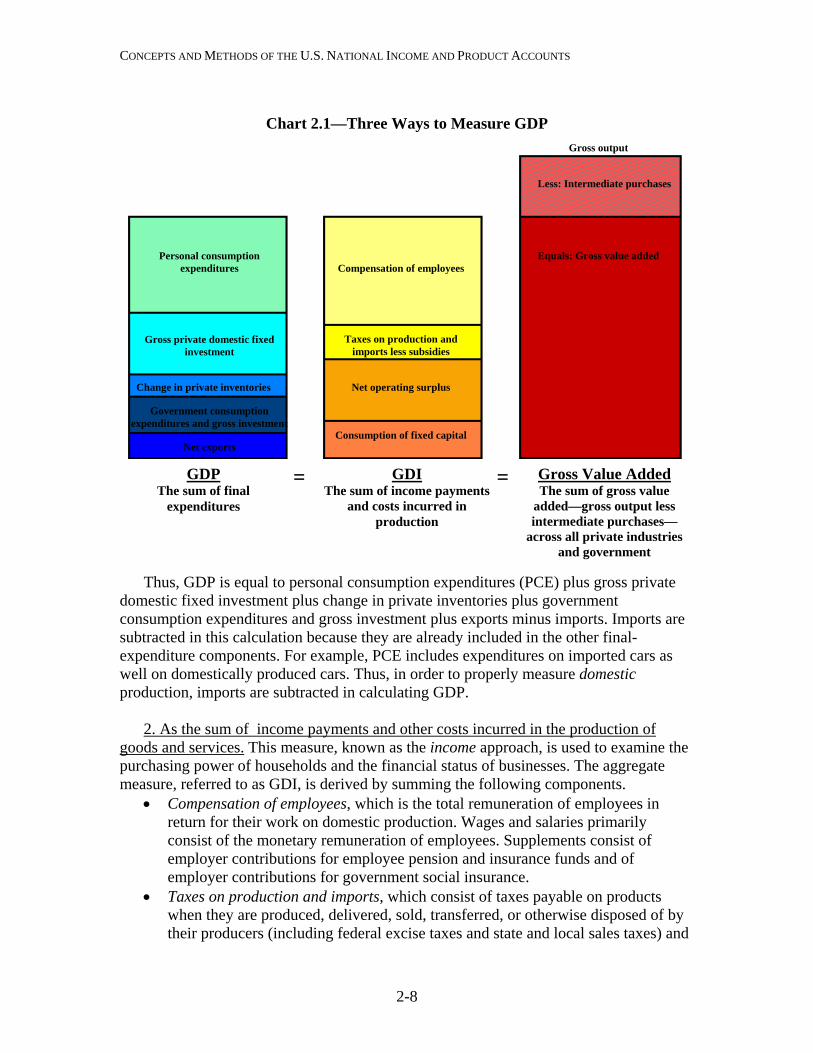
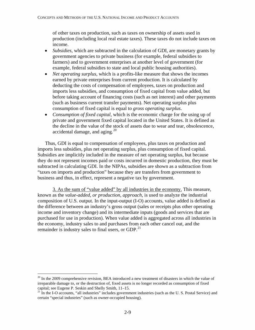
In the NIPAs, GDP is defined as the market value of the final goods and services produced by labor and property located in the United States. Conceptually, this measure can be arrived at by three separate means: as the sum of goods and services sold to final users, as the sum of income payments and other costs incurred in the production of goods and services, and as the sum of the value added at each stage of production (chart 2.1). Although these three ways of measuring GDP are conceptually the same, their calculation may not result in identical estimates of GDP because of differences in data sources, timing, and estimation techniques.
1. As the sum of goods and services sold to final users. This measure, known as the expenditures approach is used to identify the final goods and services purchased by persons, businesses, governments, and foreigners. It is arrived at by summing the following final expenditures components.
• Personal consumption expenditures, which measures the value of the goods and services purchased by persons—that is, households, nonprofit institutions that primarily serve households, private noninsured welfare funds, and private trust funds.
• Gross private fixed investment, which measures additions and replacements to the stock of private fixed assets without deduction of depreciation. Nonresidential fixed investment measures investment by businesses and nonprofit institutions in nonresidential structures and in equipment and software. Residential fixed investment measures investment by businesses and households in residential structures and equipment, primarily new construction of single-family and multifamily units.
• Change in private inventories, which measures the value of the change in the physical volume of inventories owned by private business over a specified period.
• Net exports of goods and services, which is calculated as exports less imports. Exports consist of goods and services that are sold or transferred by U.S. residents to foreign residents. Imports, which are subtracted in the calculation of GDP, consist of goods and services that are sold or transferred by foreign residents to U.S. residents.
• Government consumption expenditures and gross investment, which comprises two components. Current consumption expenditures consists of the spending by general government in order to produce and provide goods and services to the public. Gross investment consists of spending by both general government and
2-7
CONCEPTS AND METHODS OF THE U.S. NATIONAL INCOME AND PRODUCT ACCOUNTS
Chart 2.1—Three Ways to Measure GDP
Gross output
Less: Intermediate purchases
Personal consumption
expenditures
Equals: Gross value added
Compensation of employees
Gross private domestic fixed investment
Taxes on production and
imports less subsidies
Change in private inventories
Net operating surplus
Government consumption expenditures and gross investment
Consumption of fixed capital Net exports
GDI The sum of income payments
and costs incurred in production
Gross Value Added The sum of gross value
added—gross output less intermediate purchases—
across all private industries and government
= = GDP The sum of final
expenditures
Thus, GDP is equal to personal consumption expenditures (PCE) plus gross private
domestic fixed investment plus change in private inventories plus government consumption expenditures and gross investment plus exports minus imports. Imports are subtracted in this calculation because they are already included in the other final-expenditure components. For example, PCE includes expenditures on imported cars as well on domestically produced cars. Thus, in order to properly measure domestic production, imports are subtracted in calculating GDP.
2. As the sum of income payments and other costs incurred in the production of
goods and services. This measure, known as the income approach, is used to examine the purchasing power of households and the financial status of businesses. The aggregate measure, referred to as GDI, is derived by summing the following components.
• Compensation of employees, which is the total remuneration of employees in return for their work on domestic production. Wages and salaries primarily consist of the monetary remuneration of employees. Supplements consist of employer contributions for employee pension and insurance funds and of employer contributions for government social insurance.
• Taxes on production and imports, which consist of taxes payable on products when they are produced, delivered, sold, transferred, or otherwise disposed of by their producers (including federal excise taxes and state and local sales taxes) and
2-8
CONCEPTS AND METHODS OF THE U.S. NATIONAL INCOME AND PRODUCT ACCOUNTS
of other taxes on production, such as taxes on ownership of assets used in production (including local real estate taxes). These taxes do not include taxes on income.
• Subsidies, which are subtracted in the calculation of GDI, are monetary grants by government agencies to private business (for example, federal subsidies to farmers) and to government enterprises at another level of government (for example, federal subsidies to state and local public housing authorities).
• Net operating surplus, which is a profits-like measure that shows the incomes earned by private enterprises from current production. It is calculated by deducting the costs of compensation of employees, taxes on production and imports less subsidies, and consumption of fixed capital from value added, but before taking account of financing costs (such as net interest) and other payments (such as business current transfer payments). Net operating surplus plus consumption of fixed capital is equal to gross operating surplus.
• Consumption of fixed capital, which is the economic charge for the using up of private and government fixed capital located in the United States. It is defined as the decline in the value of the stock of assets due to wear and tear, obsolescence, accidental damage, and aging.20
Thus, GDI is equal to compensation of employees, plus taxes on production and
imports less subsidies, plus net operating surplus, plus consumption of fixed capital. Subsidies are implicitly included in the measure of net operating surplus, but because they do not represent incomes paid or costs incurred in domestic production, they must be subtracted in calculating GDI. In the NIPAs, subsidies are shown as a subtraction from “taxes on imports and production” because they are transfers from government to business and thus, in effect, represent a negative tax by government.
3. As the sum of “value added” by all industries in the economy. This measure, known as the value-added, or production, approach, is used to analyze the industrial composition of U.S. output. In the input-output (I-O) accounts, value added is defined as the difference between an industry’s gross output (sales or receipts plus other operating income and inventory change) and its intermediate inputs (goods and services that are purchased for use in production). When value added is aggregated across all industries in the economy, industry sales to and purchases from each other cancel out, and the remainder is industry sales to final users, or GDP.21
20 In the 2009 comprehensive revision, BEA introduced a new treatment of disasters in which the value of irreparable damage to, or the destruction of, fixed assets is no longer recorded as consumption of fixed capital; see Eugene P. Seskin and Shelly Smith, 11–15. 21 In the I-O accounts, “all industries” includes government industries (such as the U. S. Postal Service) and certain “special industries” (such as owner-occupied housing).
2-9
CONCEPTS AND METHODS OF THE U.S. NATIONAL INCOME AND PRODUCT ACCOUNTS
The I-O accounts focus on gross output because they are designed to measure the productive activities and interrelationships of all industries, regardless of whether the goods and services produced by these industries are for intermediate or for final use.
Thus, gross output is sometimes referred to as “gross duplicated domestic output,” because it double-counts the industry output that is purchased by other industries and used as inputs for their production. Because GDP counts only industry sales to final users, it is sometimes referred to as a “nonduplicative” measure of production in the economy.
To illustrate, a new car shipped from an auto assembly plant reflects not only the
costs and profit associated with final assembly but also the costs and profit associated with all of the stages of production that preceded final assembly. At an earlier stage, the tires that were put on that car were recorded as output of the tire plant and reflected the costs and profit associated with their manufacture. Thus, in gross output, the value of the tires is counted twice—once in the value of the auto manufacturer’s output and once in the value of the tire manufacturer’s output. Further, including the value of the rubber and metal that were shipped to the tire plant would constitute triple counting, and so on. In contrast, in the measurement of auto-industry value added, the value of the tires shipped to the assembly plant represents an intermediate input and so is subtracted from the value of the shipments of completed cars from the assembly plant.
Because the nation’s total value added is equal to its GDP and the nation’s total
gross output is equal to its GDP plus its total intermediate inputs, total gross output is much larger than GDP. For 2002 (the most recent benchmark year for the I-O accounts), U.S. gross output was $19.2 trillion, while GDP was $10.6 trillion.
Major NIPA aggregates
In the NIPAs, the measure of domestic production that is derived as the sum of
the final expenditures components is referred to as GDP, and the measure that is derived as the sum of the income payments and the costs incurred in production is referred to as GDI. These two measures and their components make up the “Domestic Income and Product Account,” the first of the summary NIPA accounts (see the section “Accounting Framework”). In general, the source data for the expenditures components are considered more reliable than those for the income components, and the difference between the two measures is called the “statistical discrepancy.”
2-10
CONCEPTS AND METHODS OF THE U.S. NATIONAL INCOME AND PRODUCT ACCOUNTS
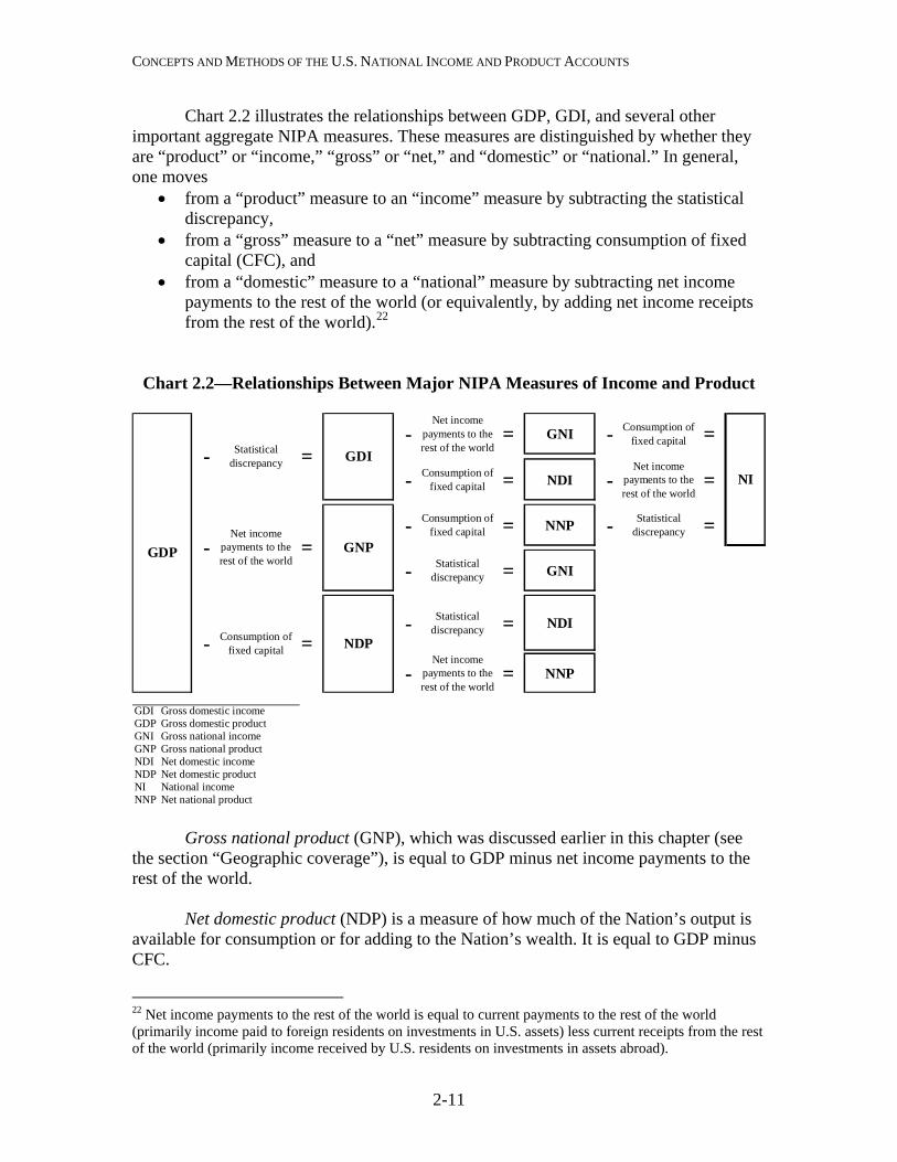
Chart 2.2 illustrates the relationships between GDP, GDI, and several other important aggregate NIPA measures. These measures are distinguished by whether they are “product” or “income,” “gross” or “net,” and “domestic” or “national.” In general, one moves
• from a “product” measure to an “income” measure by subtracting the statistical discrepancy,
• from a “gross” measure to a “net” measure by subtracting consumption of fixed capital (CFC), and
• from a “domestic” measure to a “national” measure by subtracting net income payments to the rest of the world (or equivalently, by adding net income receipts from the rest of the world).22
Chart 2.2—Relationships Between Major NIPA Measures of Income and Product
-Net income
payments to the rest of the world
= GNI - Consumption of fixed capital =
- Consumption of fixed capital = NDI -
Net income payments to the rest of the world
=
- Consumption of fixed capital = NNP - Statistical
discrepancy =
- Statistical discrepancy = GNI
- Statistical discrepancy = NDI
-Net income
payments to the rest of the world
= NNP
GDI Gross domestic incomeGDP Gross domestic productGNI Gross national incomeGNP Gross national productNDI Net domestic incomeNDP Net domestic productNI National incomeNNP Net national product
NDP
GDINI
GNP-Net income
payments to the rest of the world
=GDP
- Consumption of fixed capital =
- Statistical discrepancy =
Gross national product (GNP), which was discussed earlier in this chapter (see
the section “Geographic coverage”), is equal to GDP minus net income payments to the rest of the world.
Net domestic product (NDP) is a measure of how much of the Nation’s output is
available for consumption or for adding to the Nation’s wealth. It is equal to GDP minus CFC.
22 Net income payments to the rest of the world is equal to current payments to the rest of the world (primarily income paid to foreign residents on investments in U.S. assets) less current receipts from the rest of the world (primarily income received by U.S. residents on investments in assets abroad).
2-11
CONCEPTS AND METHODS OF THE U.S. NATIONAL INCOME AND PRODUCT ACCOUNTS
Gross national income (GNI) measures the costs incurred and the incomes earned
in the production of GNP. It is equal to GNP minus the statistical discrepancy. It is also equal to GDI minus net income payments to the rest of the world.
Net national product (NNP) is the net market value of goods and services
produced by labor and property supplied by U.S. residents (see the earlier description of GNP). It is equal to GNP minus CFC. It is also equal to NDP minus net income payments to the rest of the world.
Net domestic income (NDI) measures the costs incurred and the incomes earned in
the production of NNP. It is equal to NNP minus the statistical discrepancy. It is also equal to GDI minus CFC.
National income is the sum of all net incomes earned in production (and thus it
could also be termed “net national income”). It is equal to GNI minus CFC, NNP minus the statistical discrepancy, and NDI minus net income payments to the rest of the world. It is also equal to the sum of compensation of employees, taxes on production and imports less subsidies, and net operating surplus, minus net income payments to the rest of the world (or plus net income receipts from the rest of the world).
The following are several other important NIPA aggregates. Personal income is the income that persons receive in return for their provision of
labor, land, and capital used in current production and the net current transfer payments that they receive from business and from government.23 Personal income is equal to national income minus corporate profits with inventory valuation and capital consumption adjustments, taxes on production and imports less subsidies, contributions for government social insurance, net interest and miscellaneous payments on assets, business current transfer payments (net), current surplus of government enterprises, and wage accruals less disbursements, plus personal income receipts on assets and personal current transfer receipts.24
Gross domestic purchases is the market value of goods and services purchased by
U.S. residents, regardless of where those goods and services were produced. It is equal to GDP minus net exports. It is also equal to the sum of PCE, gross private domestic investment, and government consumption expenditures and gross investment.
Final sales of domestic product is equal to GDP less change in private
inventories. It is also equal to the sum of personal consumption expenditures, gross private fixed investment, government consumption expenditures and gross investment, and net exports of goods and services.
23 “Persons” consists of households, nonprofit institutions that primarily serve households, private noninsured welfare funds, and private trust funds. 24 For more information, see State Personal Income 2005 Methodology at www.bea.gov/regional/docs/spi2005.
2-12
CONCEPTS AND METHODS OF THE U.S. NATIONAL INCOME AND PRODUCT ACCOUNTS
Final sales to domestic purchasers is equal to gross domestic purchases less
change in private inventories. It is also equal to the sum of personal consumption expenditures, gross private fixed investment, and government consumption expenditures and gross investment.
Principal quantity and price measures
The market values and imputations used to measure GDP and the other NIPA
estimates are in current dollars—that is, they reflect transactions in terms of their value in the periods in which they take place. Although many technical problems arise in preparing these estimates, measuring the change in current-dollar GDP from one period to the next is conceptually straightforward, because it is the actual change in spending that occurs in the economy between the two time periods.
For many analyses, it is useful to separate the changes in current-dollar GDP that
are due to changes in quantity from those that are due to changes in price.25 However, aggregate quantity change and aggregate price change cannot be observed directly in the economy. Instead, these changes must be calculated, and the calculation method is determined by analytic requirements. In the NIPAs, the changes in quantities and prices are computed from chain-type indexes that are calculated using a Fisher formula. (For a discussion of the statistical methods used to prepare these measures, see “Chapter 4: Estimating Methods.”)
In the NIPAs, the featured measure of growth in the U.S. economy is the percent
change in real GDP—that is, the quantity-change measure for GDP from one period to another.26 Thus, changes in real GDP provide a comprehensive measure of economic growth that is free of the effects of price change.
In the NIPAs, the featured measure of inflation in the U.S. economy is the percent
change in the price index for gross domestic purchases. This index measures the prices of goods and services purchased by U.S. residents, regardless of where the goods and services were produced. It is derived from the prices of PCE, gross private domestic investment, and government consumption expenditures and gross investment. Thus, for example, an increase in the import price of a foreign-built car would raise the prices paid by U.S. residents and thereby directly affect the price index for gross domestic purchases.27
25 In this separation, changes in the quality of the goods and services provided are treated as changes in quantity. 26 Until 1991, GNP was the featured measure of U.S. production; see “Gross Domestic Product as a Measure of U.S. Production,” Survey 71 (August 1991): 8. 27 This example assumes the entire price increase is passed on to the car buyer—that is, the wholesale or retail margins are unchanged.
2-13
CONCEPTS AND METHODS OF THE U.S. NATIONAL INCOME AND PRODUCT ACCOUNTS
Another aggregate price measure is the price index for GDP, which measures the prices of goods and services produced in the United States. In contrast to the price index for gross domestic purchases, the GDP price index would not be directly affected by an increase in the import price of a foreign-built car, because imports are not included in GDP.
Another important NIPA price measure is the PCE price index, which measures
the prices paid for the goods and services purchased by “persons.” This index is frequently compared with the consumer price index, which is produced by the Bureau of Labor Statistics. The two indexes are similar, but there are differences in terms of coverage, weighting, and calculation.28
Further, BEA provides variants of the above price indexes that exclude their
particularly volatile food and energy components. These variants are sometimes used to indicate the “core inflation” in the U.S. economy.
BEA publishes several aggregate measures of real income as counterparts to its aggregate measures of real production. Real GDI is calculated as current-dollar GDI deflated by the implicit price deflator (IPD) for GDP; real GNI is calculated as current-dollar GNI deflated by the IPD for GNP; and real net domestic income is calculated as current-dollar net domestic income deflated by the IPD for net domestic product.29
In addition, BEA prepares alternative measures of real GDP and real GNP that
measure the real purchasing power of the income generated from the production of the goods and services by the U.S. economy. These measures, which in the NIPAs are called command-basis GDP and command-basis GNP, reflect gains or losses in real income that result from trading gains as well as from changes in production.30 In calculating command-basis GDP, exports and imports of goods and services are each deflated by the price index for gross domestic purchases to yield exports on a command-basis and imports on a command basis; then, command-basis exports are added to, and command-basis imports are subtracted from, real gross domestic purchases.31 The calculation of command-basis GNP is the same, except income receipts from the rest of the world are deflated along with exports, and income payments to the rest of the world are deflated along with imports.32 In effect, the calculations are the same as deriving command-basis 28 See Clinton P. McCully, Brian C. Moyer, and Kenneth J. Stewart, “Comparing the Consumer Price Index and the Personal Consumption Expenditures Price Index,” Survey 87 (November 2007): 26–33. 29 Implicit price deflators for an aggregate or component are calculated as the ratio of the current-dollar value to the corresponding chained-dollar value, multiplied by 100 (see the section “Chained-dollar measures” in chapter 4). 30 In the SNAs, these measures are referred to as real GDI and real GNI. However, as noted in the preceding paragraph, BEA uses a different method to derive those aggregates. 31 In this case, adding and subtracting these estimates is acceptable because all three aggregates are derived using the same deflator. 32 This methodology for calculating the command-basis aggregates was introduced in the 2010 annual revision of the NIPAs; see Eugene P. Seskin and Shelly Smith, “Annual Revision of the National Income and Product Accounts,” Survey 90 (August 2010): 21. For additional technical and historical background, see Marshall B. Reinsdorf, “Terms of Trade Effects: Theory and Measurement,” Review of Income and Wealth 56 (June 2010): S177-S205.
2-14

CONCEPTS AND METHODS OF THE U.S. NATIONAL INCOME AND PRODUCT ACCOUNTS
GDP (GNP) by deflating current-dollar GDP (GNP) by the price index for gross domestic purchases. Thus, the command-basis measures are alternative measures of real GDP and real GNP that reflect the prices of purchased goods and services, while the primary measures of real GDP and real GNP reflect the prices of produced goods and services.
BEA also prepares several measures that show the relationship between the prices that are received by U.S. producers and the prices that are paid by U.S. purchasers. The broadest measure, the trading gains index, is the ratio of the GDP price index to the price index for gross domestic purchases. An increase (decrease) in this ratio would indicate an increase (decrease) in the purchasing power of the income generated in producing GDP. Successively narrower measures specifically focus on the relationship between the prices of the U.S. goods and services that are produced for consumption by the rest of the world and the prices of the goods and services that are produced by the rest of the world for U.S. consumption. The terms of trade index, is the ratio of the price index for exports of goods and services to the price index for imports of goods and services; ratios for the terms of trade in goods and in nonpetroleum goods are also prepared. Movements in these trading indexes reflect the interaction of several factors—including movements in exchange rates, changes in the composition of traded goods and services, and changes in producers’ profit margins.
In addition, BEA provides statistical measures that supplement the current-dollar,
quantity-index, and price-index measures. Foremost among these are measures of the contributions of major components to the percent change from the preceding year or quarter in real GDP, in other principal product-side aggregates, in GDP prices, and in gross domestic purchases prices. BEA also provides measures of the percentage shares of current-dollar GDP and GDI that are accounted for by their major components.
Classification
The application of common classification systems for the NIPAs, and for all of the U.S. economic accounts, is extremely important because classification provides the structure necessary to prepare and present the estimates uniformly and consistently. Further, common classifications enable users to effectively compare and analyze data across the broad spectrum of economic statistics.
In the NIPAs, the estimates of production and expenditures may be classified by
sector, by type of product, and by function, while the estimates of income may be classified by industry and by legal form of organization. Sector
For measuring domestic production in the NIPAs, the contribution, or value added, of various institutions can be broken down into three distinct groups, or sectors—
2-15

CONCEPTS AND METHODS OF THE U.S. NATIONAL INCOME AND PRODUCT ACCOUNTS
business, households and institutions, and general government (table 2.1). A fourth sector, “the rest-of-the-world,” covers transactions between U. S. residents and foreign residents.
Table 2.1—Gross Value Added by Sector Gross domestic product Business Nonfarm Farm Households and institutions Households Nonprofit institutions serving households General government Federal State and local Note. Adapted from NIPA table 1.3.1.
Business: The business sector comprises all corporate and noncorporate businesses that are organized for profit, other entities that produce goods and services for sale at a price intended at least to approximate the costs of production, and certain other entities that are treated as businesses in the NIPAs. These other entities include mutual financial institutions, private noninsured pension funds, cooperatives, nonprofit organizations (that is, entities classified as nonprofit by the Internal Revenue Service in determining income tax liability) that primarily serve business, federal reserve banks, federally sponsored credit agencies, and government enterprises. The gross value added of the business sector is measured as GDP less the gross value added of households and institutions and of general government.33
Households and institutions: The households and institutions sector comprises
households and nonprofit institutions serving households (NPISHs). The gross value added of households is measured by the services of owner-occupied housing and the compensation paid to domestic workers. The gross value added of NPISHs is measured by the compensation paid to the employees of these institutions, the rental value of fixed assets owned and used by these institutions, and the rental income of persons for tenant-occupied housing owned by these institutions.34
General government: The general government sector comprises all federal
government and state and local government agencies except government enterprises. The gross value added of general government is measured as the sum of the compensation of the employees of these agencies and of their consumption of fixed capital.
33 Measures of gross value added for financial and for nonfinancial corporations are also shown in the NIPA tables. They are calculated based on the costs incurred and the incomes earned from production. 34 For more information on NPISHs, see the technical note in “Chapter 5: Personal Consumption Expenditures.”
2-16
CONCEPTS AND METHODS OF THE U.S. NATIONAL INCOME AND PRODUCT ACCOUNTS
Type of product
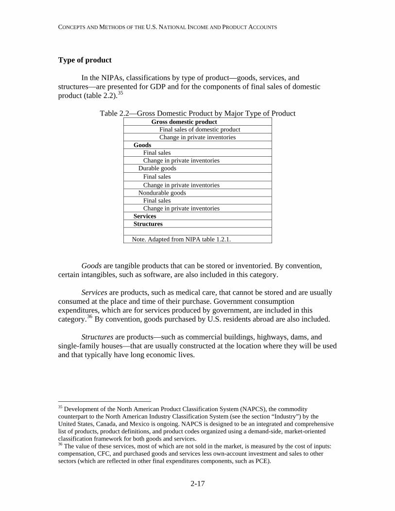
In the NIPAs, classifications by type of product—goods, services, and structures—are presented for GDP and for the components of final sales of domestic product (table 2.2).35
Table 2.2—Gross Domestic Product by Major Type of Product
Gross domestic product Final sales of domestic product Change in private inventories Goods Final sales Change in private inventories Durable goods Final sales Change in private inventories Nondurable goods Final sales Change in private inventories Services Structures Note. Adapted from NIPA table 1.2.1.
Goods are tangible products that can be stored or inventoried. By convention, certain intangibles, such as software, are also included in this category.
Services are products, such as medical care, that cannot be stored and are usually
consumed at the place and time of their purchase. Government consumption expenditures, which are for services produced by government, are included in this category.36 By convention, goods purchased by U.S. residents abroad are also included.
Structures are products—such as commercial buildings, highways, dams, and
single-family houses—that are usually constructed at the location where they will be used and that typically have long economic lives.
35 Development of the North American Product Classification System (NAPCS), the commodity counterpart to the North American Industry Classification System (see the section “Industry”) by the United States, Canada, and Mexico is ongoing. NAPCS is designed to be an integrated and comprehensive list of products, product definitions, and product codes organized using a demand-side, market-oriented classification framework for both goods and services. 36 The value of these services, most of which are not sold in the market, is measured by the cost of inputs: compensation, CFC, and purchased goods and services less own-account investment and sales to other sectors (which are reflected in other final expenditures components, such as PCE).
2-17
CONCEPTS AND METHODS OF THE U.S. NATIONAL INCOME AND PRODUCT ACCOUNTS
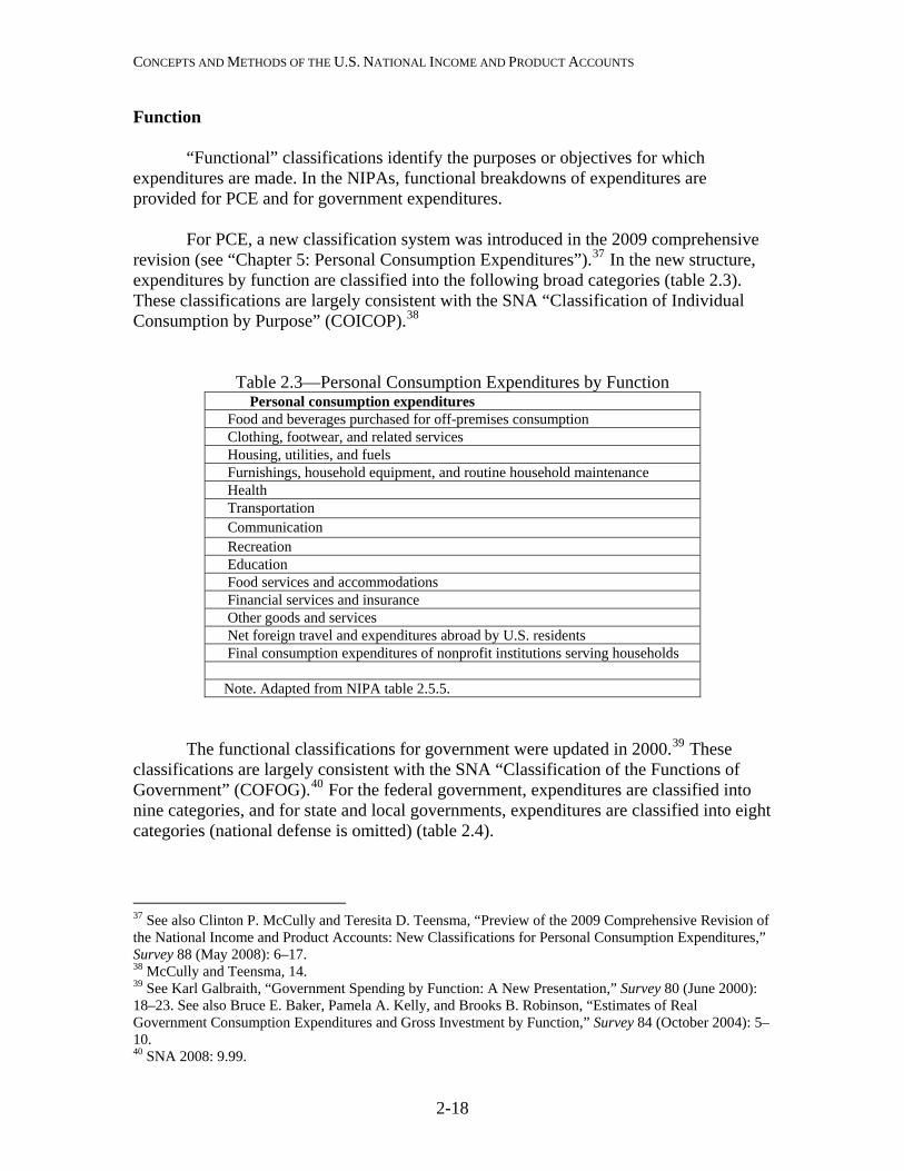
Function “Functional” classifications identify the purposes or objectives for which
expenditures are made. In the NIPAs, functional breakdowns of expenditures are provided for PCE and for government expenditures.
For PCE, a new classification system was introduced in the 2009 comprehensive
revision (see “Chapter 5: Personal Consumption Expenditures”).37 In the new structure, expenditures by function are classified into the following broad categories (table 2.3). These classifications are largely consistent with the SNA “Classification of Individual Consumption by Purpose” (COICOP).38
Table 2.3—Personal Consumption Expenditures by Function Personal consumption expenditures Food and beverages purchased for off-premises consumption Clothing, footwear, and related services Housing, utilities, and fuels Furnishings, household equipment, and routine household maintenance Health Transportation Communication Recreation Education Food services and accommodations Financial services and insurance Other goods and services Net foreign travel and expenditures abroad by U.S. residents Final consumption expenditures of nonprofit institutions serving households Note. Adapted from NIPA table 2.5.5.
The functional classifications for government were updated in 2000.39 These
classifications are largely consistent with the SNA “Classification of the Functions of Government” (COFOG).40 For the federal government, expenditures are classified into nine categories, and for state and local governments, expenditures are classified into eight categories (national defense is omitted) (table 2.4).
37 See also Clinton P. McCully and Teresita D. Teensma, “Preview of the 2009 Comprehensive Revision of the National Income and Product Accounts: New Classifications for Personal Consumption Expenditures,” Survey 88 (May 2008): 6–17. 38 McCully and Teensma, 14. 39 See Karl Galbraith, “Government Spending by Function: A New Presentation,” Survey 80 (June 2000): 18–23. See also Bruce E. Baker, Pamela A. Kelly, and Brooks B. Robinson, “Estimates of Real Government Consumption Expenditures and Gross Investment by Function,” Survey 84 (October 2004): 5–10. 40 SNA 2008: 9.99.
2-18
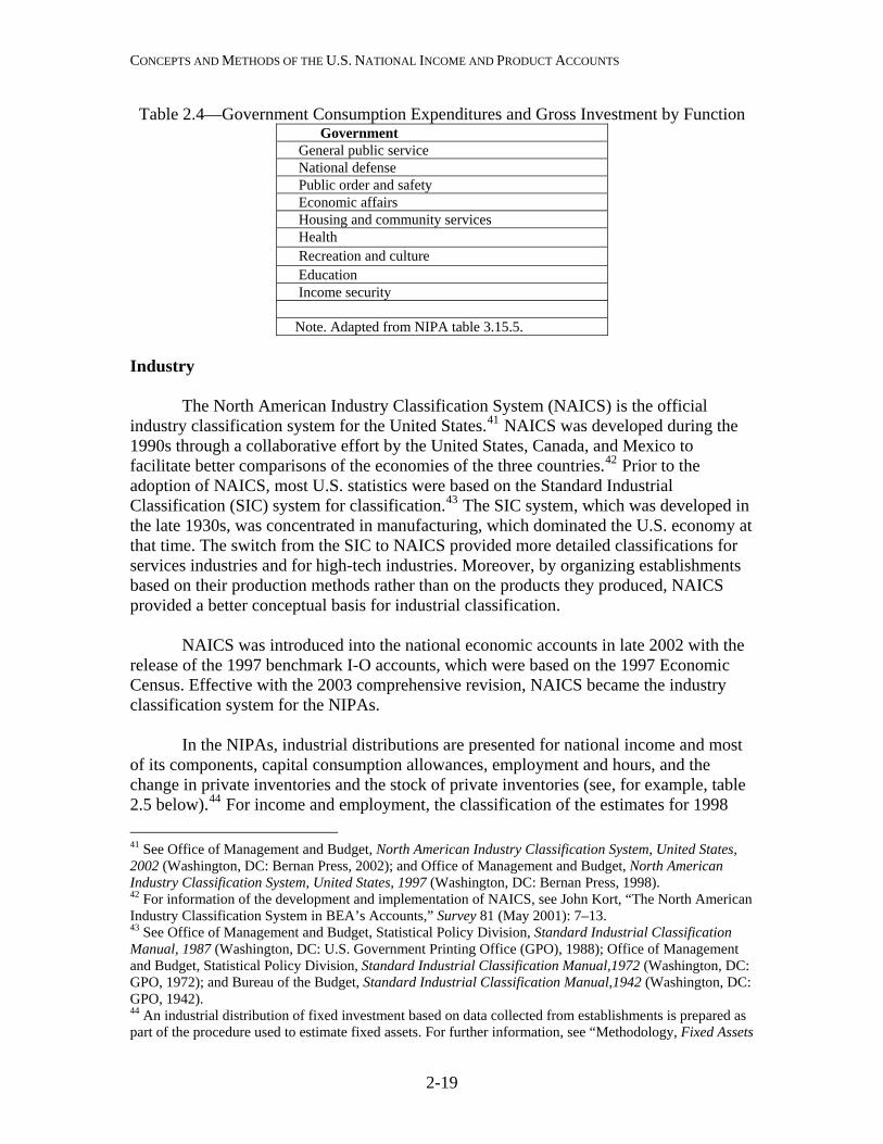
CONCEPTS AND METHODS OF THE U.S. NATIONAL INCOME AND PRODUCT ACCOUNTS
Table 2.4—Government Consumption Expenditures and Gross Investment by Function Government General public service National defense Public order and safety Economic affairs Housing and community services Health Recreation and culture Education Income security Note. Adapted from NIPA table 3.15.5.
Industry
The North American Industry Classification System (NAICS) is the official
industry classification system for the United States.41 NAICS was developed during the 1990s through a collaborative effort by the United States, Canada, and Mexico to facilitate better comparisons of the economies of the three countries.42 Prior to the adoption of NAICS, most U.S. statistics were based on the Standard Industrial Classification (SIC) system for classification.43 The SIC system, which was developed in the late 1930s, was concentrated in manufacturing, which dominated the U.S. economy at that time. The switch from the SIC to NAICS provided more detailed classifications for services industries and for high-tech industries. Moreover, by organizing establishments based on their production methods rather than on the products they produced, NAICS provided a better conceptual basis for industrial classification.
NAICS was introduced into the national economic accounts in late 2002 with the release of the 1997 benchmark I-O accounts, which were based on the 1997 Economic Census. Effective with the 2003 comprehensive revision, NAICS became the industry classification system for the NIPAs.
In the NIPAs, industrial distributions are presented for national income and most of its components, capital consumption allowances, employment and hours, and the change in private inventories and the stock of private inventories (see, for example, table 2.5 below).44 For income and employment, the classification of the estimates for 1998 41 See Office of Management and Budget, North American Industry Classification System, United States, 2002 (Washington, DC: Bernan Press, 2002); and Office of Management and Budget, North American Industry Classification System, United States, 1997 (Washington, DC: Bernan Press, 1998). 42 For information of the development and implementation of NAICS, see John Kort, “The North American Industry Classification System in BEA’s Accounts,” Survey 81 (May 2001): 7–13. 43 See Office of Management and Budget, Statistical Policy Division, Standard Industrial Classification Manual, 1987 (Washington, DC: U.S. Government Printing Office (GPO), 1988); Office of Management and Budget, Statistical Policy Division, Standard Industrial Classification Manual,1972 (Washington, DC: GPO, 1972); and Bureau of the Budget, Standard Industrial Classification Manual,1942 (Washington, DC: GPO, 1942). 44 An industrial distribution of fixed investment based on data collected from establishments is prepared as part of the procedure used to estimate fixed assets. For further information, see “Methodology, Fixed Assets
2-19
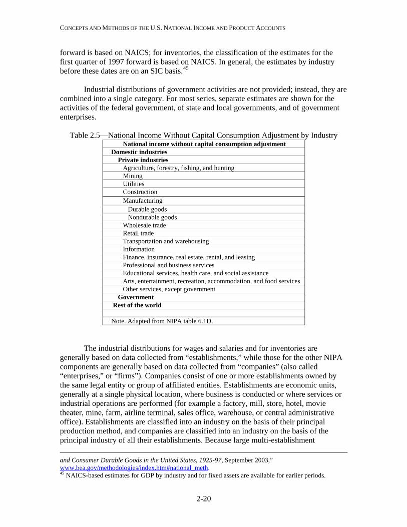
CONCEPTS AND METHODS OF THE U.S. NATIONAL INCOME AND PRODUCT ACCOUNTS
forward is based on NAICS; for inventories, the classification of the estimates for the first quarter of 1997 forward is based on NAICS. In general, the estimates by industry before these dates are on an SIC basis.45
Industrial distributions of government activities are not provided; instead, they are
combined into a single category. For most series, separate estimates are shown for the activities of the federal government, of state and local governments, and of government enterprises.
Table 2.5—National Income Without Capital Consumption Adjustment by Industry
National income without capital consumption adjustment Domestic industries Private industries Agriculture, forestry, fishing, and hunting Mining Utilities Construction Manufacturing Durable goods Nondurable goods Wholesale trade Retail trade Transportation and warehousing Information Finance, insurance, real estate, rental, and leasing Professional and business services Educational services, health care, and social assistance Arts, entertainment, recreation, accommodation, and food services Other services, except government Government Rest of the world Note. Adapted from NIPA table 6.1D.
The industrial distributions for wages and salaries and for inventories are
generally based on data collected from “establishments,” while those for the other NIPA components are generally based on data collected from “companies” (also called “enterprises,” or “firms”). Companies consist of one or more establishments owned by the same legal entity or group of affiliated entities. Establishments are economic units, generally at a single physical location, where business is conducted or where services or industrial operations are performed (for example a factory, mill, store, hotel, movie theater, mine, farm, airline terminal, sales office, warehouse, or central administrative office). Establishments are classified into an industry on the basis of their principal production method, and companies are classified into an industry on the basis of the principal industry of all their establishments. Because large multi-establishment and Consumer Durable Goods in the United States, 1925-97, September 2003,” www.bea.gov/methodologies/index.htm#national_meth. 45 NAICS-based estimates for GDP by industry and for fixed assets are available for earlier periods.
2-20
CONCEPTS AND METHODS OF THE U.S. NATIONAL INCOME AND PRODUCT ACCOUNTS
companies typically contain establishments that are classified in different industries, the industrial distribution of the same economic activity on an establishment basis can differ significantly from that on a company basis. For example, the measure of employment by steel-manufacturing companies will include the employment of establishments that do not manufacture steel but are part of companies that are classified as steel-manufacturing companies. Similarly, this measure will exclude the employment of establishments that manufacture steel but are part of companies that are not classified as steel-manufacturing companies.
Moreover, individual industry series are not fully comparable over time. First, the
composition of industries may change because of revisions to NAICS or to the SIC. This factor affects estimates based on establishment data and on company data. Second, historical comparability may be affected by a change over time in the industrial classification of the same establishment or company. For example, the classification of a company may change as a result of shifts in the level of consolidation of entities for which company reports are filed or as a result of mergers and acquisitions. This factor affects company-based estimates much more than establishment-based estimates.
In addition, some NIPA tables show the following special industry groupings: Financial industries consists of the NAICS industry “Finance and insurance” and
of “Offices of bank holding companies” and “Offices of other holding companies” in the NAICS industry “Management of companies and enterprises.” Finance and insurance consists of Federal Reserve banks; credit intermediation and related activities; securities, commodity contracts, and investments; insurance carriers and related activities; and funds, trusts, and other financial vehicles.
Nonfinancial industries consists of all other private industries. Private goods-producing industries consists of the following NAICS divisions:
agriculture, forestry, fishing, and hunting; mining; construction; and manufacturing. Private services-producing industries consists of the following NAICS divisions:
utilities; wholesale trade; retail trade; transportation and warehousing; information; finance and insurance; real estate and rental and leasing; professional, scientific, and technical services; management of companies and enterprises; administrative and waste management services; educational services; health care and social assistance; arts, entertainment, and recreation; accommodation and food services; and other services, except government. Legal form of organization
For the domestic business sector in the NIPAs, classification by legal form of organization is shown for national income and its components. Legal forms of organization are based on IRS filing requirements for corporate business and for
2-21
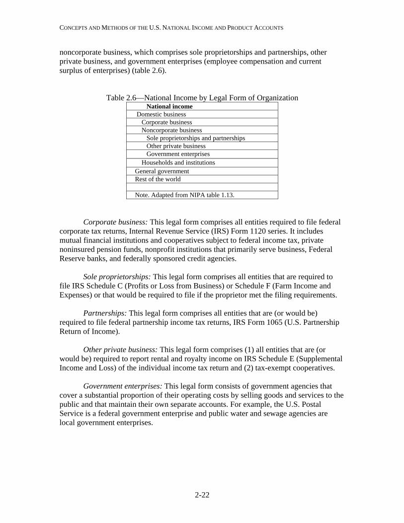
CONCEPTS AND METHODS OF THE U.S. NATIONAL INCOME AND PRODUCT ACCOUNTS
noncorporate business, which comprises sole proprietorships and partnerships, other private business, and government enterprises (employee compensation and current surplus of enterprises) (table 2.6).
Table 2.6—National Income by Legal Form of Organization National income Domestic business Corporate business Noncorporate business Sole proprietorships and partnerships Other private business Government enterprises Households and institutions General government Rest of the world Note. Adapted from NIPA table 1.13.
Corporate business: This legal form comprises all entities required to file federal
corporate tax returns, Internal Revenue Service (IRS) Form 1120 series. It includes mutual financial institutions and cooperatives subject to federal income tax, private noninsured pension funds, nonprofit institutions that primarily serve business, Federal Reserve banks, and federally sponsored credit agencies.
Sole proprietorships: This legal form comprises all entities that are required to
file IRS Schedule C (Profits or Loss from Business) or Schedule F (Farm Income and Expenses) or that would be required to file if the proprietor met the filing requirements.
Partnerships: This legal form comprises all entities that are (or would be)
required to file federal partnership income tax returns, IRS Form 1065 (U.S. Partnership Return of Income).
Other private business: This legal form comprises (1) all entities that are (or
would be) required to report rental and royalty income on IRS Schedule E (Supplemental Income and Loss) of the individual income tax return and (2) tax-exempt cooperatives.
Government enterprises: This legal form consists of government agencies that
cover a substantial proportion of their operating costs by selling goods and services to the public and that maintain their own separate accounts. For example, the U.S. Postal Service is a federal government enterprise and public water and sewage agencies are local government enterprises.
2-22

CONCEPTS AND METHODS OF THE U.S. NATIONAL INCOME AND PRODUCT ACCOUNTS
Accounting Framework
The NIPAs consist of a set of integrated accounts that provide statistics on the output of the U.S. economy. The NIPA accounting framework is designed to provide context for these statistics, so that they are presented logically, consistently, and according to established economic-accounting principles and standards. The NIPAs are generally consistent with the SNA, which now serves as the internationally accepted set of guidelines for the compilation of national accounts.46
For an in-depth discussion of the conceptual framework of the NIPAs and the NIPA summary accounts, see U.S. Bureau of Economic Analysis, An Introduction to National Economic Accounting, Methodology Paper No. 1 (updated), September 2007.
Accounting principles Double-entry bookkeeping is one of the most fundamental principles used in economic accounting and in financial accounting. In financial accounting, activities that affect the resources available to a business are recorded at least once as a source of financing (credit) and at least once as a use of financing (debit). Thus, double-entry bookkeeping provides a means to validate the accounting entries, because the sum of the entries on each side of an account must be equal. In national economic accounting, each transaction is recorded as a payment by one sector and as a receipt by the same sector or by another sector—for example corporate income tax is a payment by a corporation and a receipt of the government.47 In addition to providing a means to validate entries, this system also provides alternative ways to calculate a measure when complete information is not available for one of the sectors.
The accrual-accounting method is another principle important to both financial
and economic accounting. This method is generally used to ensure that related revenues and expenses are recorded in the same accounting period. In accrual accounting, revenues are recorded when they are earned, and expenses are recorded when they are incurred, regardless of when the cash is actually received or paid. The accrual-accounting method may be contrasted to the cash-accounting method, which records revenues when cash is received and expenses when cash is paid.
Financial accounting and economic accounting generally apply different
principles in valuing transactions. In financial accounting, assets (and depreciation) are commonly valued at historical costs—that is, at the prices relevant at the time of the acquisition; subsequent changes in the value of these assets are ignored. In economic 46 See Charles Ian Mead, Karin E. Moses, and Brent R. Moulton, “The NIPAs and the System of National Accounts,” Survey 84 (December 2004): 17–32. 47 A fully articulated set of national accounts (showing payments and receipts by all sectors) actually leads to a quadruple-entry system (in which each transaction is recorded as a debit and a change in in assets for one sector and as a credit and a change in assets for another sector) . However transactions are usually recorded only twice in the NIPAs because the changes in assets or liabilities that are associated with the changes in revenues or expenses are recorded in the Federal Reserve Board’s flow of funds accounts.
2-23
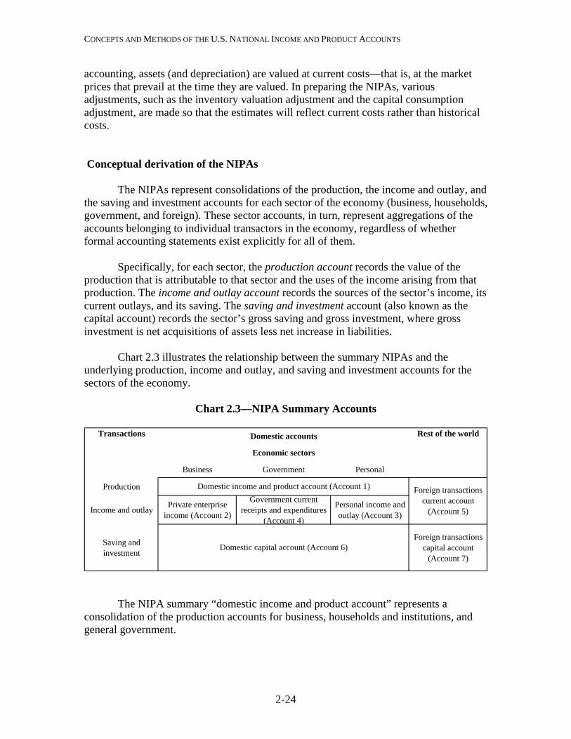
CONCEPTS AND METHODS OF THE U.S. NATIONAL INCOME AND PRODUCT ACCOUNTS
accounting, assets (and depreciation) are valued at current costs—that is, at the market prices that prevail at the time they are valued. In preparing the NIPAs, various adjustments, such as the inventory valuation adjustment and the capital consumption adjustment, are made so that the estimates will reflect current costs rather than historical costs.
Conceptual derivation of the NIPAs The NIPAs represent consolidations of the production, the income and outlay, and the saving and investment accounts for each sector of the economy (business, households, government, and foreign). These sector accounts, in turn, represent aggregations of the accounts belonging to individual transactors in the economy, regardless of whether formal accounting statements exist explicitly for all of them. Specifically, for each sector, the production account records the value of the production that is attributable to that sector and the uses of the income arising from that production. The income and outlay account records the sources of the sector’s income, its current outlays, and its saving. The saving and investment account (also known as the capital account) records the sector’s gross saving and gross investment, where gross investment is net acquisitions of assets less net increase in liabilities. Chart 2.3 illustrates the relationship between the summary NIPAs and the underlying production, income and outlay, and saving and investment accounts for the sectors of the economy.
Chart 2.3—NIPA Summary Accounts
Business Government Personal
Production
Income and outlay Private enterprise income (Account 2)
Government current receipts and expenditures
(Account 4)
Personal income and outlay (Account 3)
Saving and investment
Foreign transactions capital account
(Account 7)Domestic capital account (Account 6)
Domestic accounts
Economic sectors
Foreign transactions current account
(Account 5)
Rest of the worldTransactions
Domestic income and product account (Account 1)
The NIPA summary “domestic income and product account” represents a consolidation of the production accounts for business, households and institutions, and general government.
2-24
CONCEPTS AND METHODS OF THE U.S. NATIONAL INCOME AND PRODUCT ACCOUNTS
The income and outlay accounts for the sectors are shown in three separate summary accounts. Income and outlays for the personal sector, including income accruing to unincorporated businesses, are shown in the “personal income and outlay account.” Income and outlays for the government sector, including income accruing to government enterprises, are shown in the “government current receipts and expenditures account. Income and outlays for business enterprises and for households and institutions in their role as producers are shown in the “private enterprise income account.” In order to provide analytically useful aggregates associated with all private business, the coverage in this account includes the income and outlays of unincorporated businesses as well as those of corporate businesses. The saving and investment accounts are consolidated into a single summary “domestic capital account.” For saving, a breakdown by sector is shown for corporate, personal, and government saving. For investment, because of source data limitations, the breakdown is shown for private fixed and inventory investment and for government fixed investment. The transactions for the foreign (or rest-of-the-world) “sector”—that is, transactions between U.S. residents and foreign residents—are shown separately in two summary accounts. Current receipts and expenditures, such as exports and imports of goods and services, are shown in the “foreign transactions current account,” and capital transactions, such as capital transfers, are shown in the “foreign transactions capital account.” The summary NIPAs The seven summary NIPAs constitute the accounting framework for presenting the value of production, distribution, consumption, and saving for the U.S. economy.48 (For a full presentation of the summary accounts, see table 2.A at the end of this chapter.) Each of the entries in a summary account also appears again in that account or in one of the other summary accounts; most of these entries are also shown in one or more of the tables that make up the full set of NIPA tables. For example, the item “supplements to wages and salaries” is shown in line 5 of summary account 1 and in line 14 of summary account 3; it is also shown in line 8 of NIPA table 1.10 and in line 6 of NIPA table 2.1.
Taken together, the summary accounts constitute a double-entry system in which a use (or expenditure) recorded in one account for one sector is also recorded as a source (or receipt) in an account of another sector or of the same sector. This system of integrated, double-entry accounts provides a comprehensive measure of economic activity in a consistently defined framework without double-counting. Thus, the NIPAs,
48 Prior to the 2003 comprehensive revision, the NIPAs were summarized in five accounts, as shown in table A on pages 38–39 of the August 2002 Survey. For a discussion of the differences between the old and new summary accounts, see Nicole Mayerhauser, Shelly Smith, and David F. Sullivan, “Preview of the 2003 Comprehensive Revision of the National Income and Product Accounts: New and Redesigned Tables,” Survey 83 (August 2003): 8–15.
2-25
CONCEPTS AND METHODS OF THE U.S. NATIONAL INCOME AND PRODUCT ACCOUNTS
in combination with BEA’s industry, wealth, and other economic accounts, can be used to trace the principal economic flows among the major sectors of the economy. Account 1: Domestic Income and Product Account
This account represents an aggregation of the underlying production accounts for the domestic sectors of the U.S. economy. The right (product) side of the account shows GDP measured as the sum of goods and services sold to final users rather than as the sum of value-added by the sectors. The left (income) side of the account shows GDP as measured by the incomes earned in production—GDI—plus the “statistical discrepancy” (the difference between GDP and GDI). Product and income are both presented on a domestic basis—that is, they are produced by labor and property located in the United States. Account 2: Private Enterprise Income Account
This account presents information on the sources and uses of the income of private businesses and other private enterprises.49 It combines the accounts of private businesses, of homeowners for owner-occupied housing (which is treated as if it were a business), and of NPISHs.
Sources of private enterprise income—such as interest receipts on assets and net
operating surplus—are shown on the right side of the account.50 The left side of the account shows the uses of income as income payments on assets (such as holders of financial liabilities and equity claims of other businesses), business current transfer payments, and income that accrues to the owners of business (namely proprietors’ income, rental income of persons, and corporate profits. Corporate profits, a widely used measure in the United States, is distributed to government (taxes on corporate income) and to shareholders (net dividends) or is retained (undistributed profits, which can be thought of as a measure of corporate saving). Account 3: Personal Income and Outlay Account
This account shows the sources and uses of income received by persons—that is, households, NPISHs, private noninsured welfare funds, and private trust funds. The right side of the account shows the sources of personal income—such as employee compensation and interest and dividend income. The left side shows personal taxes and
49 Government enterprises are not included in account 2, because complete estimates on sources and uses of government enterprise income, notably the income payments and income receipts on assets, are not currently available. The sources and uses of government enterprise income are included, but not separately identified, in the government receipts and expenditures account. 50 Summary account 2 presents the components of private enterprise income on a national basis—that is, for income accruing to U.S. residents. Consequently, for the net operating surplus to be shown in account 2 on a domestic basis consistent with summary account 1, several components showing income flows to and from the rest of the world are added to account 2.
2-26
CONCEPTS AND METHODS OF THE U.S. NATIONAL INCOME AND PRODUCT ACCOUNTS
2-27
outlays and personal saving, which is derived as personal income minus personal taxes and outlays. Account 4: Government Receipts and Expenditures Account
This account summarizes the combined transactions of the federal government and of the state and local governments. The right side of the account shows government current receipts—such as tax receipts from persons and contributions for government social insurance. The left side shows government current expenditures—such as compensation of government employees and transfer payments to persons—and net saving, which is derived as current receipts less current expenditures. Account 5: Foreign Transactions Current Account
This account summarizes all the current transactions between the United States and the rest of the world. It presents information on receipts and payments associated with foreign trade and other transactions not involving transfers of assets. The left side of the account shows current receipts from the rest of the world—mainly exports of goods and services and income receipts on assets. The right side shows current payments to the rest of the world—mainly imports of goods and services, income payments on assets, and current taxes and transfer payments. In addition, it includes the balance on current account, which is derived as current receipts less current payments. Account 6: Domestic Capital Account
This account presents information on saving and investment for the economy. The right side of the account shows gross saving and the statistical discrepancy. Given the theoretical equality between GDP and GDI, the statistical discrepancy can be viewed as actual (positive or negative) income that is not captured by the data used to measure GDI and, therefore, not distributed to the sectors; instead, it is shown as a source of (positive or negative) saving in this account. The left side of the account shows gross domestic investment, capital-account transactions (net), and net lending or net borrowing, which is derived as gross saving and the statistical discrepancy minus gross domestic investment and capital-account transactions (net). Account 7: Foreign Transactions Capital Account
This account presents information on transactions between the United States and the rest of the world that are linked to the acquisition or disposition of nonproduced nonfinancial assets and capital transfers. The left side of the account shows the balance on current account. The right side shows capital-account transactions (net) and net lending or borrowing, which is derived as the balance on current account minus capital-account transactions (net).

Concepts and Methods of the U.S. National Income and Product Accounts
Table A. Summary National Income and Product Accounts, 2009[Billions of dollars]
Account 1. Domestic Income and Product Account
Line Line
1 Compensation of employees, paid ......................................................................... 7,819.5 15 Personal consumption expenditures (3–3) ............................................................ 10,001.32 Wage and salary accruals.................................................................................. 6,286.9 16 Goods ................................................................................................................ 3,230.73 Disbursements (3–12 plus 5–11) ................................................................... 6,281.9 17 Durable goods ............................................................................................... 1,026.54 Wage accruals less disbursements (4–9 plus 6–13)...................................... 5.0 18 Nondurable goods ......................................................................................... 2,204.25 Supplements to wages and salaries (3–14) ....................................................... 1,532.6 19 Services............................................................................................................. 6,770.66 Taxes on production and imports (4–16) ................................................................ 1,024.7 20 Gross private domestic investment........................................................................ 1,589.27 Less: Subsidies (4–8)............................................................................................. 60.3 21 Fixed investment (6–2) ...................................................................................... 1,716.48 Net operating surplus............................................................................................. 3,294.9 22 Nonresidential................................................................................................ 1,364.49 Private enterprises (2–19).................................................................................. 3,308.1 23 Structures .................................................................................................. 451.6
10 Current surplus of government enterprises (4–26) ............................................ –13.2 24 Equipment and software............................................................................ 912.811 Consumption of fixed capital (6–13)....................................................................... 1,861.1 25 Residential..................................................................................................... 352.1
26 Change in private inventories (6–4)................................................................... –127.212 Gross domestic income ...................................................................................... 13,939.9 27 Net exports of goods and services ........................................................................ –386.4
28 Exports (5–1)..................................................................................................... 1,578.413 Statistical discrepancy (6–21) ................................................................................ 179.1 29 Imports (5–9) ..................................................................................................... 1,964.7
30 Government consumption expenditures and gross investment (4–1 plus 6–3) ..... 2,914.931 Federal............................................................................................................... 1,139.632 National defense............................................................................................ 771.633 Nondefense ................................................................................................... 368.034 State and local................................................................................................... 1,775.3
14 GROSS DOMESTIC PRODUCT............................................................................ 14,119.0 35 GROSS DOMESTIC PRODUCT ........................................................................... 14,119.0
Account 2. Private Enterprise Income Account
Line Line
1 Income payments on assets................................................................................... 3,000.4 19 Net operating surplus, private enterprises (1–9) ................................................... 3,308.12 Interest and miscellaneous payments (3–20 and 4–21) .................................... 2,872.1 20 Income receipts on assets ..................................................................................... 2,370.23 Dividend payments to the rest of the world (5–14)............................................. 99.5 21 Interest (3–20) ................................................................................................... 1,889.64 Reinvested earnings on foreign direct investment in the United States (5–15) 28.8 22 Dividend receipts from the rest of the world (5–6)............................................. 206.85 Business current transfer payments (net) .............................................................. 134.0 23 Reinvested earnings on U.S. direct investment abroad (5–7)............................ 273.86 To persons (net) (3–24) ...................................................................................... 36.07 To government (net) (4–24)................................................................................ 98.58 To the rest of the world (net) (5–19) ................................................................... –0.69 Proprietors’ income with inventory valuation and capital consumption
adjustments (3–17) ............................................................................................ 1,011.910 Rental income of persons with capital consumption adjustment (3–18) ................ 274.011 Corporate profits with inventory valuation and capital consumption adjustments 1,258.012 Taxes on corporate income ................................................................................ 254.913 To government (4–17) .................................................................................... 231.414 To the rest of the world (5–19) ....................................................................... 23.415 Profits after tax with inventory valuation and capital consumption adjustments 1,003.116 Net dividends (3–21 plus 4–22) ..................................................................... 718.917 Undistributed corporate profits with inventory valuation and capital
consumption adjustments (6–12)............................................................... 284.2
18 USES OF PRIVATE ENTERPRISE INCOME ........................................................ 5,678.4 24 SOURCES OF PRIVATE ENTERPRISE INCOME................................................ 5,678.4
Account 3. Personal Income and Outlay Account
Line Line
1 Personal current taxes (4–15) ................................................................................ 1,140.0 10 Compensation of employees, received .................................................................. 7,806.72 Personal outlays ..................................................................................................... 10,379.6 11 Wage and salary disbursements ....................................................................... 6,274.13 Personal consumption expenditures (1–15) ....................................................... 10,001.3 12 Domestic (1–3 less 5–11).............................................................................. 6,271.24 Personal interest payments (3–20) .................................................................... 216.8 13 Rest of the world (5–3) .................................................................................. 2.95 Personal current transfer payments ................................................................... 161.4 14 Supplements to wages and salaries (1–5) ........................................................ 1,532.66 To government (4–25) .................................................................................... 95.0 15 Employer contributions for employee pension and insurance funds.............. 1,072.07 To the rest of the world (net) (5–17) ............................................................... 66.5 16 Employer contributions for government social insurance............................... 460.6
8 Personal saving (6–11) .......................................................................................... 655.317 Proprietors’ income with inventory valuation and capital consumption
adjustments (2–9).............................................................................................. 1,011.918 Rental income of persons with capital consumption adjustment (2–10)................ 274.019 Personal income receipts on assets ...................................................................... 1,919.720 Personal interest income (2–2 plus 3–4 plus 4–7 plus 5–5 less 2–21 less 4–21
less 5–13) ...................................................................................................... 1,222.321 Personal dividend income (2–16 less 4–22)...................................................... 697.422 Personal current transfer receipts .......................................................................... 2,132.823 Government social benefits (4–4)...................................................................... 2,096.824 From business (net) (2–6).................................................................................. 36.025 Less: Contributions for government social insurance, domestic (4–19) ................ 970.3
9 PERSONAL TAXES, OUTLAYS, AND SAVING.................................................... 12,174.9 26 PERSONAL INCOME ........................................................................................... 12,174.9
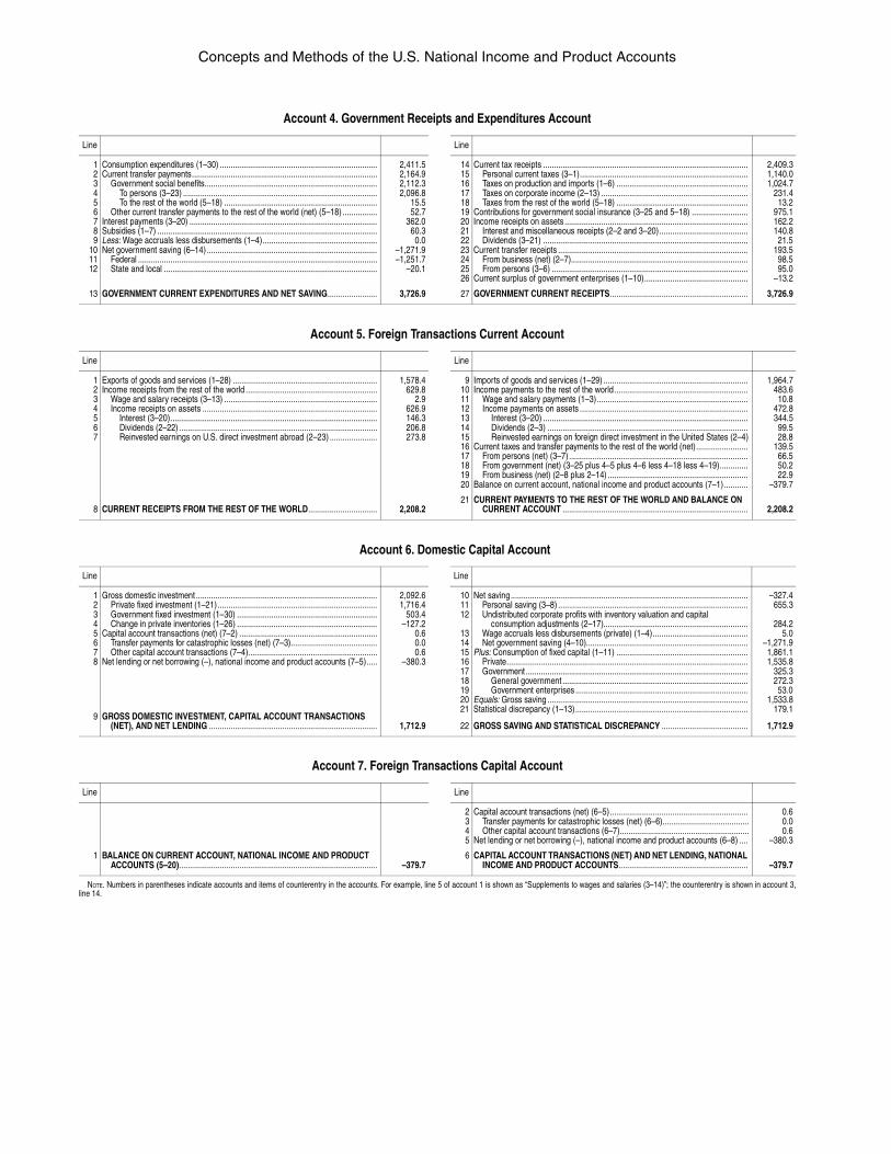
Concepts and Methods of the U.S. National Income and Product Accounts
Account 4. Government Receipts and Expenditures Account
Line Line
1 Consumption expenditures (1–30) ......................................................................... 2,411.5 14 Current tax receipts ............................................................................................... 2,409.32 Current transfer payments...................................................................................... 2,164.9 15 Personal current taxes (3–1).............................................................................. 1,140.03 Government social benefits................................................................................ 2,112.3 16 Taxes on production and imports (1–6) ............................................................. 1,024.74 To persons (3–23) .......................................................................................... 2,096.8 17 Taxes on corporate income (2–13) .................................................................... 231.45 To the rest of the world (5–18) ....................................................................... 15.5 18 Taxes from the rest of the world (5–18) ............................................................. 13.26 Other current transfer payments to the rest of the world (net) (5–18) ................ 52.7 19 Contributions for government social insurance (3–25 and 5–18) .......................... 975.17 Interest payments (3–20) ....................................................................................... 362.0 20 Income receipts on assets ..................................................................................... 162.28 Subsidies (1–7) ...................................................................................................... 60.3 21 Interest and miscellaneous receipts (2–2 and 3–20)......................................... 140.89 Less: Wage accruals less disbursements (1–4)..................................................... 0.0 22 Dividends (3–21) ............................................................................................... 21.5
10 Net government saving (6–14) ............................................................................... –1,271.9 23 Current transfer receipts ........................................................................................ 193.511 Federal ............................................................................................................... –1,251.7 24 From business (net) (2–7).................................................................................. 98.512 State and local ................................................................................................... –20.1 25 From persons (3–6) ........................................................................................... 95.0
26 Current surplus of government enterprises (1–10)................................................ –13.2
13 GOVERNMENT CURRENT EXPENDITURES AND NET SAVING....................... 3,726.9 27 GOVERNMENT CURRENT RECEIPTS................................................................ 3,726.9
Account 5. Foreign Transactions Current Account
Line Line
1 Exports of goods and services (1–28) ................................................................... 1,578.4 9 Imports of goods and services (1–29) ................................................................... 1,964.72 Income receipts from the rest of the world ............................................................. 629.8 10 Income payments to the rest of the world.............................................................. 483.63 Wage and salary receipts (3–13) ....................................................................... 2.9 11 Wage and salary payments (1–3)...................................................................... 10.84 Income receipts on assets ................................................................................. 626.9 12 Income payments on assets .............................................................................. 472.85 Interest (3–20)................................................................................................ 146.3 13 Interest (3–20) ............................................................................................... 344.56 Dividends (2–22) ............................................................................................ 206.8 14 Dividends (2–3) ............................................................................................. 99.57 Reinvested earnings on U.S. direct investment abroad (2–23) ...................... 273.8 15 Reinvested earnings on foreign direct investment in the United States (2–4) 28.8
16 Current taxes and transfer payments to the rest of the world (net)........................ 139.517 From persons (net) (3–7)................................................................................... 66.518 From government (net) (3–25 plus 4–5 plus 4–6 less 4–18 less 4–19)............. 50.219 From business (net) (2–8 plus 2–14) ................................................................. 22.920 Balance on current account, national income and product accounts (7–1) ........... –379.7
8 CURRENT RECEIPTS FROM THE REST OF THE WORLD................................ 2,208.221 CURRENT PAYMENTS TO THE REST OF THE WORLD AND BALANCE ON
CURRENT ACCOUNT ...................................................................................... 2,208.2
Line
1 Gross domestic investment .................................................................................... 2,092.62 Private fixed investment (1–21).......................................................................... 1,716.43 Government fixed investment (1–30) ................................................................. 503.44 Change in private inventories (1–26) ................................................................. –127.25 Capital account transactions (net) (7–2) ................................................................ 0.66 Transfer payments for catastrophic losses (net) (7–3)........................................ 0.07 Other capital account transactions (7–4)............................................................ 0.68 Net lending or net borrowing (–), national income and product accounts (7–5)..... –380.3
9 GROSS DOMESTIC INVESTMENT, CAPITAL ACCOUNT TRANSACTIONS (NET), AND NET LENDING .............................................................................. 1,712.9
Line
10 Net saving.............................................................................................................. –327.411 Personal saving (3–8) ........................................................................................ 655.312 Undistributed corporate profits with inventory valuation and capital
consumption adjustments (2–17)................................................................... 284.213 Wage accruals less disbursements (private) (1–4)............................................ 5.014 Net government saving (4–10)........................................................................... –1,271.915 Plus: Consumption of fixed capital (1–11) ............................................................. 1,861.116 Private................................................................................................................ 1,535.817 Government ....................................................................................................... 325.318 General government ...................................................................................... 272.319 Government enterprises ................................................................................ 53.020 Equals: Gross saving ............................................................................................. 1,533.821 Statistical discrepancy (1–13)................................................................................ 179.1
22 GROSS SAVING AND STATISTICAL DISCREPANCY ........................................ 1,712.9
Account 6. Domestic Capital Account
Account 7. Foreign Transactions Capital Account
Line Line
2 Capital account transactions (net) (6–5)................................................................ 0.63 Transfer payments for catastrophic losses (net) (6–6)........................................ 0.04 Other capital account transactions (6–7)............................................................ 0.65 Net lending or net borrowing (–), national income and product accounts (6–8) .... –380.3
1 BALANCE ON CURRENT ACCOUNT, NATIONAL INCOME AND PRODUCT ACCOUNTS (5–20)............................................................................................ –379.7
6 CAPITAL ACCOUNT TRANSACTIONS (NET) AND NET LENDING, NATIONAL INCOME AND PRODUCT ACCOUNTS............................................................ –379.7
NOTE. Numbers in parentheses indicate accounts and items of counterentry in the accounts. For example, line 5 of account 1 is shown as “Supplements to wages and salaries (3–14)”; the counterentry is shown in account 3,line 14.
CHAPTER 3: PRINCIPAL SOURCE DATA Source data as determinants of initial release and revision schedules Source data for the current quarterly estimates Source data for the annual revisions Source data for the comprehensive revisions Source data are the information BEA uses to prepare the NIPA estimates, and estimating methods are the steps BEA takes to transform the source data into these estimates. The interaction of source data and estimating methods determines the accuracy, reliability, and relevancy of the accounts. The data that BEA uses are collected from a variety of sources and are usually collected for purposes other than for incorporation into BEA's estimates. Data collected by federal government agencies provide the backbone of the estimates; these data are supplemented by data from trade associations, businesses, international organizations, and other sources. The Government data are from a number of agencies, including the Commerce Department's Bureau of the Census, the Labor Department's Bureau of Labor Statistics (BLS), the Treasury Department, the Office of Management and Budget, and the Agriculture Department. “Administrative” data are data that are tabulated by federal government and by state and local government agencies as a byproduct of administering their programs—such as processing corporate tax returns, regulating public utilities, and issuing building permits. “Statistical” data are data collected by the federal statistical agencies, such as the Census Bureau and BLS. These data consist of periodic economic and population censuses and a wide range of sample surveys, such as those that collect data on manufacturing and trade, employment, and prices. The relatively few surveys that BEA conducts cover international trade in services and international direct investment, both by foreign companies in the United States and by U.S. companies in foreign countries. The source data available to BEA are not always ideal for the preparation of the NIPAs. BEA must develop methods that transform the best available data into estimates that are consistent with the NIPA concepts and framework and that fill gaps in the coverage of the source data. (See “Chapter 4: Estimating Methods.”) Source data as determinants of initial release and revision schedules The availability of the source data is an important consideration in determining the schedules for the initial release and the subsequent revisions of the NIPA estimates. One factor affecting availability is the speed with which the source data are collected, compiled, and released. Another factor is whether the source data are part of a statistical program that, over time, provides more complete or otherwise better coverage—for
3-1
CONCEPTS AND METHODS OF THE U.S. NATIONAL INCOME AND PRODUCT ACCOUNTS
example, if the sample is larger or if more detailed information is collected for an annual survey than for the monthly surveys. In general, the most comprehensive source data for the expenditure components of GDP are available at the 5-year intervals associated with the economic census of establishments conducted by the Census Bureau. The economic census is the primary data source for BEA’s input-output accounts, which are used to "benchmark" the NIPA estimates for the quinquennial census years—most recently, 1997 and 2002. Related annual surveys are drawn from samples of the establishments covered in the economic census; these surveys generally collect less detailed data than those collected in the economic census. Many of the annual surveys are supplemented by monthly surveys that involve smaller samples and that collect less detailed data than the annual surveys.1 In addition, responding to the censuses and annual surveys is generally mandatory, while responding to most of the quarterly and monthly surveys is voluntary.
The data from the monthly surveys are available first, and they provide much of the information that is used to prepare the initial, or “current,” quarterly (and for a few components, monthly) NIPA estimates. These estimates are subsequently revised as additional reports become available from the monthly surveys. Annual revisions, which are timed to incorporate newly available annual source data, are usually carried out each summer. Comprehensive revisions, which incorporate the most complete source data as well as other improvements to the accounts, are carried out at about 5-year intervals.
The following sections describe the most important federal government source
data that are used for the current quarterly estimates and for the annual and comprehensive revisions of the NIPAs. In the preparation of the estimates, these sources are augmented by a wealth of information from other public sources and from private sources, such as trade associations.
Source data for the current quarterly estimates
Data from Census Bureau monthly surveys are among the primary sources for the current quarterly estimates (table 3.1). For the most part, the samples for these voluntary surveys are drawn from the economic census, from the corresponding annual surveys, and from the Business Register; the samples are updated periodically to account for new businesses (“births”) and for businesses that discontinue operations (“deaths”).2
1 Many of the annual and monthly surveys are based on “probability sampling” (sometimes known as “scientific sampling”). In this process, establishments are first placed into various “strata” on the basis of their size. Depending on the distribution of establishments, an establishment in the largest strata could have a 100-percent probability of selection and thus have a sampling weight of 1—that is, the establishment would represent only itself. An establishment in a smaller stratum would have a smaller probability of selection, say 1 percent, but in that case the establishment would have a sampling weight of 100—that is, the sampled establishment would represent 100 establishments. 2 The Business Register is a comprehensive database of U.S. business establishments and companies that is maintained by the Census Bureau for statistical program use. A “business” is defined as legal or administrative entity that is assigned an employer identification number (EIN) by the Internal Revenue Service.
3-2
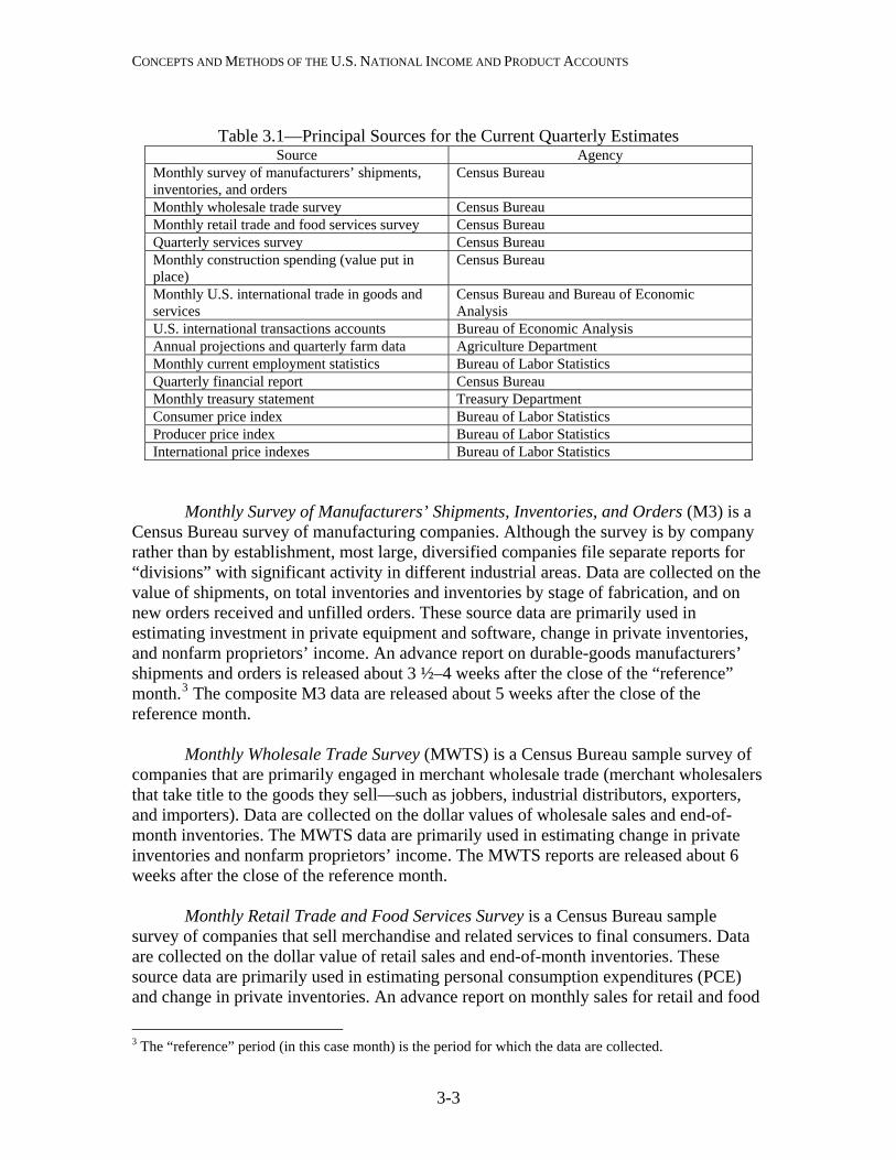
CONCEPTS AND METHODS OF THE U.S. NATIONAL INCOME AND PRODUCT ACCOUNTS
Table 3.1—Principal Sources for the Current Quarterly Estimates
Source Agency Monthly survey of manufacturers’ shipments, inventories, and orders
Census Bureau
Monthly wholesale trade survey Census Bureau Monthly retail trade and food services survey Census Bureau Quarterly services survey Census Bureau Monthly construction spending (value put in place)
Census Bureau
Monthly U.S. international trade in goods and services
Census Bureau and Bureau of Economic Analysis
U.S. international transactions accounts Bureau of Economic Analysis Annual projections and quarterly farm data Agriculture Department Monthly current employment statistics Bureau of Labor Statistics Quarterly financial report Census Bureau Monthly treasury statement Treasury Department Consumer price index Bureau of Labor Statistics Producer price index Bureau of Labor Statistics International price indexes Bureau of Labor Statistics
Monthly Survey of Manufacturers’ Shipments, Inventories, and Orders (M3) is a Census Bureau survey of manufacturing companies. Although the survey is by company rather than by establishment, most large, diversified companies file separate reports for “divisions” with significant activity in different industrial areas. Data are collected on the value of shipments, on total inventories and inventories by stage of fabrication, and on new orders received and unfilled orders. These source data are primarily used in estimating investment in private equipment and software, change in private inventories, and nonfarm proprietors’ income. An advance report on durable-goods manufacturers’ shipments and orders is released about 3 ½–4 weeks after the close of the “reference” month.3 The composite M3 data are released about 5 weeks after the close of the reference month. Monthly Wholesale Trade Survey (MWTS) is a Census Bureau sample survey of companies that are primarily engaged in merchant wholesale trade (merchant wholesalers that take title to the goods they sell—such as jobbers, industrial distributors, exporters, and importers). Data are collected on the dollar values of wholesale sales and end-of-month inventories. The MWTS data are primarily used in estimating change in private inventories and nonfarm proprietors’ income. The MWTS reports are released about 6 weeks after the close of the reference month. Monthly Retail Trade and Food Services Survey is a Census Bureau sample survey of companies that sell merchandise and related services to final consumers. Data are collected on the dollar value of retail sales and end-of-month inventories. These source data are primarily used in estimating personal consumption expenditures (PCE) and change in private inventories. An advance report on monthly sales for retail and food
3 The “reference” period (in this case month) is the period for which the data are collected.
3-3
CONCEPTS AND METHODS OF THE U.S. NATIONAL INCOME AND PRODUCT ACCOUNTS
services (MARTS) is released about 1 ½–2 weeks after the close of the reference month. The composite retail sales and inventories data are released about 6 weeks after the close of the reference month. Quarterly Services Survey (QSS) is a Census Bureau sample survey that was initiated in 2003–2004 in order to improve the coverage of the service industries in the U.S. economy. Since 2004, the QSS has collected data on total revenue for companies in the following service sectors in the North American Industry Classification System: information; professional, scientific, and technical; administrative and support and waste management and remediation; and hospitals and nursing and residential care facilities. In 2009, coverage was expanded to the following services: transportation and warehousing; rental and leasing; ambulatory health care; social assistance; arts, entertainment, and recreation; other services (except public administration); and finance and insurance. The QSS data are primarily used in estimating PCE and investment in private equipment and software. The QSS data are released about 2 ½ months after the close of the reference quarter. Monthly construction spending (value put-in-place) is a Census Bureau measure of the value of construction installed or erected during a given period. The data for private nonresidential buildings, for government structures, and for multifamily residential buildings are derived from data collected by sampling the owners of construction projects.4 The data for single-family residential buildings are derived indirectly using information collected in a series of sample surveys that track the number of housing-unit permits, starts, sales, and completions. The data for “other construction” are derived from a variety of sources covering farm, utility, communication, and railroad structures. These source data are primarily used in estimating private and government investment in structures. The data for construction put-in-place are released about 1 month after the close of the reference month. Monthly U.S. international trade in goods and services consist of Census Bureau estimates of trade in goods and BEA estimates of trade in services. The Census Bureau tabulations of exported and imported goods are from documents filed with Customs and Border Protection, U.S. Department of Homeland Security; they cover all shipments above a certain size and a sample of the remaining shipments. The BEA estimates are primarily based on 11 mandatory BEA surveys of selected services receipts, payments, and other data. These data are supplemented by a combination of monthly indicator source data, partial data from U.S. Government agencies and from foreign central statistical offices and banks, and other secondary source data. These source data are primarily used in estimating private investment in equipment and software and in estimating exports and imports. The U.S. international trade statistics are jointly released by the two agencies 6-7 weeks after the close of the reference month.
4 In contrast, the census of construction, which is part of the economic census, measures construction on the basis of reports by establishments primarily engaged in construction. Thus, value put-in-place captures some important parts of construction activity that are not included in the census—such as nonemployer construction, architectural and engineering costs, own-account construction, homeowner construction, and construction done as a secondary source of revenue by nonconstruction establishments.
3-4
CONCEPTS AND METHODS OF THE U.S. NATIONAL INCOME AND PRODUCT ACCOUNTS
International Transactions Accounts (ITAs), prepared by BEA, summarize the quarterly transactions between the United States and the rest of the world. In the ITAs, the current account records exports and imports of goods and services, receipts and payments of income on assets, and unilateral transfers (net gifts to other countries). In the capital and financial account, the capital account records capital transfers (such as debt forgiveness) and the financial account records transactions involving exchanges of financial assets for other financial assets or for tangible resources and gifts or grants of financial assets. These source data are primarily used in estimating corporate profits. The ITAs are released about 2 ½ months after the close of the reference quarter. Annual projections and quarterly farm data, from the U.S. Department of Agriculture, consist of annual projections of crop output, quarterly projections of cash receipts and of inventories for livestock, and annual projections of government subsidy payments and production expenses for both crops and livestock. These data are primarily used in estimating change in private inventories and farm proprietors’ income. Monthly Current Employment Statistics (CES) survey is a sample survey of business establishments that is conducted by state employment security agencies in cooperation with BLS. The CES (also known as BLS-790) covers payroll employment in private nonagricultural industries during the pay period that includes the 12th of the month. The data collected include series for total employment, number of production or nonsupervisory workers, average hourly earnings, average weekly hours, average weekly earnings, and average weekly overtime hours in manufacturing industries. (BLS has developed experimental series that extend coverage to all employees and that include irregular payments, such as bonuses.) These source data are primarily used in estimating PCE, wages and salaries, and nonfarm proprietors’ income. The CES data are usually released on the first Friday following the close of the reference month. Quarterly Financial Report (QFR), prepared by the Census Bureau, provides aggregate statistics on the financial position of U.S. corporations. Based on a sample survey of firms above specified asset sizes, the QFR presents estimated statements of income and retained earnings, balance sheets, and related financial and operating ratios for manufacturing, mining, and trade corporations by industry and by asset size. These source data are primarily used in estimating corporate profits. The QFR statistics for manufacturing, mining, and wholesale trade are released about 2 ½ months after the close of the reference quarter, and the statistics for retail trade are released about 1 month later. Monthly Treasury Statement (MTS), prepared by the Financial Management Service of the U.S. Department of the Treasury, summarizes the financial activities of the federal government and off-budget federal entities in accordance with the Budget of the U.S. Government. The MTS presents a summary of receipts and outlays, surplus or deficit, and means of financing. The data are provided by federal entities, disbursing officers, and Federal Reserve Banks. These source data are primarily used in estimating federal government receipts and expenditures and federal government consumption
3-5
CONCEPTS AND METHODS OF THE U.S. NATIONAL INCOME AND PRODUCT ACCOUNTS
expenditures and gross investment. The MTS is released about 2 weeks after the close of the reference month. Consumer Price Index (CPI), prepared by BLS, is a family of indexes that measure the average monthly change in the prices paid by urban consumers for a fixed market basket of goods and services. The CPI covers “out-of-pocket” expenditures, including user fees (such as water and sewer service) and sales and excise taxes paid by the consumer but excluding income taxes and investment items (such as stocks, bonds, and life insurance). The CPI is estimated from a statistical set of samples of urban areas, of consumers within those areas, of retailers and other outlets, and of specific, unique items purchased. CPIs are primarily used in deflating PCE, change in private inventories, and state and local government purchases. The CPI is released 2–3 weeks after the close of the reference month. Producer Price Index (PPI), prepared by BLS, is a family of indexes that measure the average monthly change in prices received by domestic producers of goods and services. Thus, the PPI measures price change from the perspective of the seller rather than the purchaser. The PPI covers practically the entire output of domestic goods-producing sectors and is expanding its coverage of services and other non-goods-producing sectors. The PPI is estimated from data collected from a sample of establishments that participate in the Unemployment Insurance System, a joint federal and state program that covers about 97 percent of wage and salary workers. PPIs are primarily used in deflating private investment in equipment and software and in structures, change in private inventories, government purchases, and exports and imports. The PPI is released about 2 weeks after the close of the reference month.
International Price Indexes, prepared by BLS, measure monthly changes in the prices of goods and services that are sold by U.S. producers to foreign buyers (exports) and that are purchased from abroad by U.S. buyers (imports). The price indexes for exports of goods to Canada are based primarily on sampling information obtained from the Canadian Customs Service, and the indexes for exports of goods to other countries are based on sampling information obtained from the U.S. Census Bureau. The price indexes for imports of goods are based on sampling information obtained from Customs and Border Protection, U.S. Department of Homeland Security. The price indexes for exports and imports of services are based on sampling information that is developed separately for each service category. These price indexes are primarily used in deflating private investment in equipment and software, change in private inventories, and exports and imports. The international price indexes are released about 2 weeks after the close of the reference month. Estimating schedule For GDP and most other NIPA series, the estimates for each quarter are prepared on a schedule that calls for three successive "current" estimates—"advance," "second,"
3-6
CONCEPTS AND METHODS OF THE U.S. NATIONAL INCOME AND PRODUCT ACCOUNTS
and "third."5 The specific release date for each month is primarily determined by the availability of the monthly reports on retail sales, manufacturing shipments, and international trade in goods from the Census Bureau (along with the time it takes BEA to process them).
• The advance quarterly estimate of GDP is released near the end of the month that follows the close of the reference quarter. For most of the product-side components, the estimate is based on source data for either 2 or 3 months of the quarter. In most cases, however, the source data for the second and third months of the quarter are subject to revision by the issuing agencies. Where source data are not available, the estimate is based primarily on BEA projections. For an example of how this information is provided in the Survey of Current Business, see the box “Summary of Source Data for the Advance Estimates of GDP” on page 8 (which was adapted from “GDP and the Economy” in the August 2008 Survey).
• One month later, the advance estimate is replaced by the second estimate, which is typically based on source data for all 3 months of the quarter. However, in some instances, the source data used for the second estimate, particularly the data for the third month of the quarter, are subject to further revision.
• One month later, the second estimate is replaced by the third estimate, which incorporates revisions to source data for the third month of the quarter and newly available quarterly source data for some components.
For certain “income-side” series—gross national product, gross domestic income,
national income, and corporate profits—“advance” estimates are not prepared, because of a lag in the availability of source data. For the first, second, and third quarters of the year, the release of the second GDP estimate presents the initial estimates for these income-side series, and the third GDP release presents revised estimates. For the fourth quarter, the estimates for these series are presented only in the third GDP release.
In addition, when the second estimate of GDP for the current quarter is released,
the preceding quarter’s estimates of private wages and salaries and affected income-side aggregates are revised to incorporate newly available preliminary tabulations from the BLS quarterly census of employment and wages (QCEW).6 (For a description of the QCEW, see the section on source data for annual revisions.)
5 In the 2009 comprehensive revision of the NIPAs, BEA introduced new names for the second two vintages of the current quarterly estimates. Formerly, the “second” estimate was known as the “preliminary” estimate, and the “third” estimate” was known as the “final” estimate. The initial estimate continues to be named the “advance” estimate. (See Eugene P. Seskin and Shelly Smith, “Preview of the 2009 Comprehensive Revision of the NIPAs: Changes in Definitions and Presentations,” Survey of Current Business 89 (March 2009): 19–20.) 6 Affected aggregates include gross domestic income, the statistical discrepancy, gross national income, national income, personal income, disposable personal income, personal saving, gross (national) saving, compensation, and gross product of corporate business. Other components that are closely linked to wages and salaries, such as personal current taxes and employer contributions for government social insurance, are also revised. Product-side series, including GDP, are not affected.
3-7
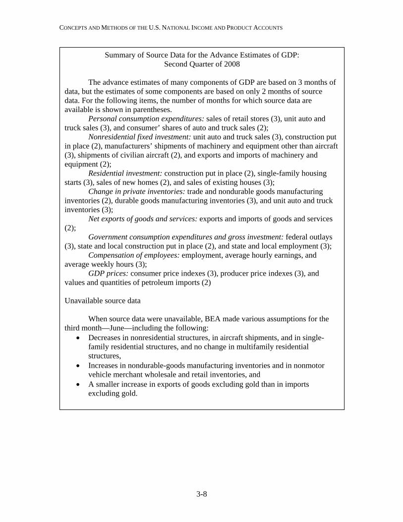
CONCEPTS AND METHODS OF THE U.S. NATIONAL INCOME AND PRODUCT ACCOUNTS
Summary of Source Data for the Advance Estimates of GDP: Second Quarter of 2008
The advance estimates of many components of GDP are based on 3 months of
data, but the estimates of some components are based on only 2 months of source data. For the following items, the number of months for which source data are available is shown in parentheses. Personal consumption expenditures: sales of retail stores (3), unit auto and truck sales (3), and consumer’ shares of auto and truck sales (2); Nonresidential fixed investment: unit auto and truck sales (3), construction put in place (2), manufacturers’ shipments of machinery and equipment other than aircraft (3), shipments of civilian aircraft (2), and exports and imports of machinery and equipment (2); Residential investment: construction put in place (2), single-family housing starts (3), sales of new homes (2), and sales of existing houses (3); Change in private inventories: trade and nondurable goods manufacturing inventories (2), durable goods manufacturing inventories (3), and unit auto and truck inventories (3); Net exports of goods and services: exports and imports of goods and services (2); Government consumption expenditures and gross investment: federal outlays (3), state and local construction put in place (2), and state and local employment (3); Compensation of employees: employment, average hourly earnings, and average weekly hours (3); GDP prices: consumer price indexes (3), producer price indexes (3), and values and quantities of petroleum imports (2) Unavailable source data When source data were unavailable, BEA made various assumptions for the third month—June—including the following:
• Decreases in nonresidential structures, in aircraft shipments, and in single-family residential structures, and no change in multifamily residential structures,
• Increases in nondurable-goods manufacturing inventories and in nonmotor vehicle merchant wholesale and retail inventories, and
• A smaller increase in exports of goods excluding gold than in imports excluding gold.
3-8
CONCEPTS AND METHODS OF THE U.S. NATIONAL INCOME AND PRODUCT ACCOUNTS
Source-data categories The source data used to prepare the quarterly estimates of the product-side components of GDP can be grouped into four general categories based on their quality, availability, and use.7
• Revised monthly or quarterly data are based on revised monthly or quarterly source data; they are presumed to be more accurate than preliminary data.
• Initial monthly or quarterly data include either monthly data for all 3 months of a quarter or data for a complete quarter.
• Monthly data and trend-based data typically include source data for the first 2 months but limited or no data for the third month; for the third month, BEA makes a projection based on various assumptions.
• Trend-based data are typically projections that are calculated by BEA using previous estimates and trends, moving averages of various lengths, regressions, and judgment by BEA economists.
For the advance GDP estimate, initial monthly or quarterly data account for 46
percent of the source data used to calculate the estimates. Monthly data and trend-based data account for 30 percent, and trend-based data account for the remainder. (See chart 3.1 on the next page).
For the second and third GDP estimates, most of the monthly data and trend-based data are replaced by revised monthly or quarterly data, which are generally considered more accurate. The revised data account for 72 percent of the source data for those estimates. For the second estimate, most of the remainder is accounted for by trend-based data, at 24 percent. For the third estimate, however, most of the remainder is accounted for by initial monthly or quarterly data, at 20 percent.
The estimates of new residential structures provide an example of the progression
of source data from the advance quarterly estimate to the third quarterly estimate. The advance estimate of new residential structures incorporates source data for the first and second months of the quarter and an assumption for the third month; these source data are categorized as monthly data and trend-based data. The second estimate incorporates revised data for the first and second months and newly available data for the third month; these source data are categorized as revised monthly or quarterly data. The third estimate incorporates data for the second and third months that are revised further; these source data are also categorized as revised monthly or quarterly data.
7 For more information, see Bruce T. Grimm and Teresa L. Weadock, “Gross Domestic Product: Revisions and Source Data,” Survey 86 (February 2006): 11–15.
3-9
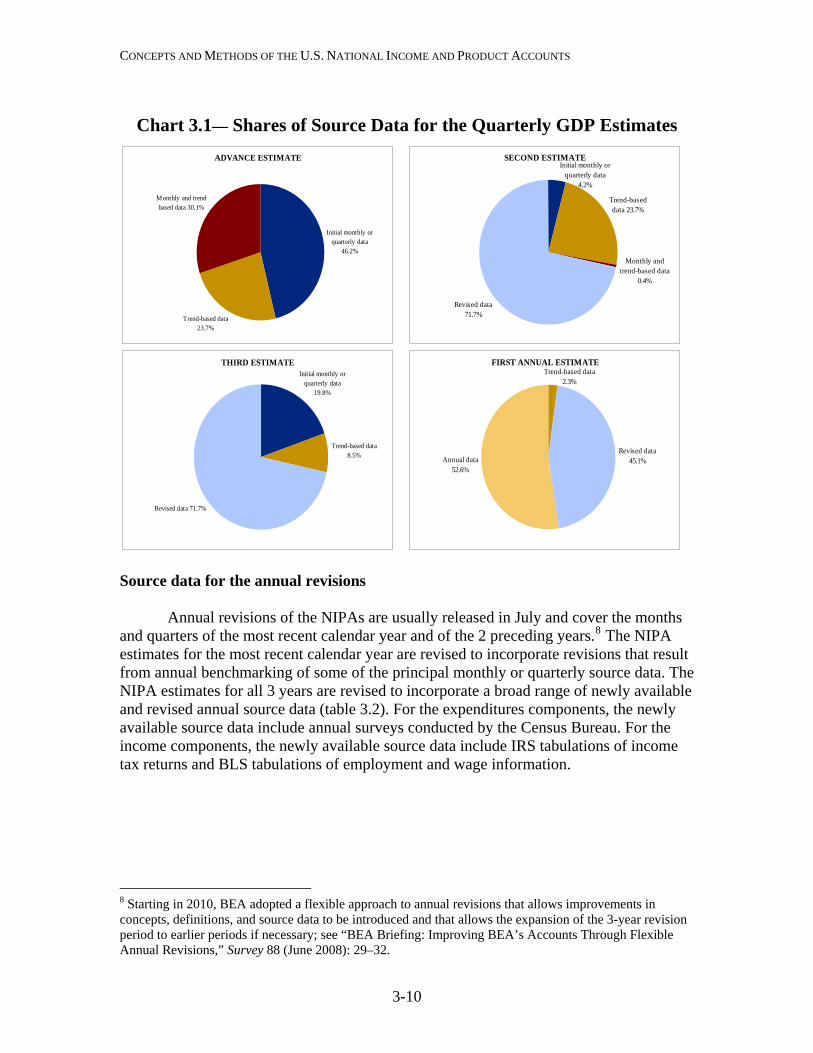
CONCEPTS AND METHODS OF THE U.S. NATIONAL INCOME AND PRODUCT ACCOUNTS
Chart 3.1— Shares of Source Data for the Quarterly GDP Estimates
ADVANCE ESTIMATE
Trend-based data 23.7%
Monthly and trend-based data 30.1%
Initial monthly or quarterly data
46.2%
SECOND ESTIMATE
Trend-based data 23.7%
Monthly and trend-based data
0.4%
Revised data 71.7%
Initial monthly or quarterly data
4.2%
FIRST ANNUAL ESTIMATE
Revised data 45.1%Annual data
52.6%
Trend-based data 2.3%
THIRD ESTIMATE
Trend-based data 8.5%
Revised data 71.7%
Initial monthly or quarterly data
19.8%
Source data for the annual revisions
Annual revisions of the NIPAs are usually released in July and cover the months and quarters of the most recent calendar year and of the 2 preceding years.8 The NIPA estimates for the most recent calendar year are revised to incorporate revisions that result from annual benchmarking of some of the principal monthly or quarterly source data. The NIPA estimates for all 3 years are revised to incorporate a broad range of newly available and revised annual source data (table 3.2). For the expenditures components, the newly available source data include annual surveys conducted by the Census Bureau. For the income components, the newly available source data include IRS tabulations of income tax returns and BLS tabulations of employment and wage information.
8 Starting in 2010, BEA adopted a flexible approach to annual revisions that allows improvements in concepts, definitions, and source data to be introduced and that allows the expansion of the 3-year revision period to earlier periods if necessary; see “BEA Briefing: Improving BEA’s Accounts Through Flexible Annual Revisions,” Survey 88 (June 2008): 29–32.
3-10
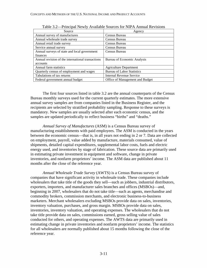
CONCEPTS AND METHODS OF THE U.S. NATIONAL INCOME AND PRODUCT ACCOUNTS
Table 3.2—Principal Newly Available Sources for NIPA Annual Revisions Source Agency
Annual survey of manufactures Census Bureau Annual wholesale trade survey Census Bureau Annual retail trade survey Census Bureau Service annual survey Census Bureau Annual surveys of state and local government finances
Census Bureau
Annual revision of the international transactions accounts
Bureau of Economic Analysis
Annual farm statistics Agriculture Department Quarterly census of employment and wages Bureau of Labor Statistics Tabulations of tax returns Internal Revenue Service Federal government annual budget Office of Management and Budget
The first four sources listed in table 3.2 are the annual counterparts of the Census Bureau monthly surveys used for the current quarterly estimates. The more extensive annual survey samples are from companies listed in the Business Register, and the recipients are selected by stratified probability sampling. Response to these surveys is mandatory. New samples are usually selected after each economic census, and the samples are updated periodically to reflect business “births” and “deaths.” Annual Survey of Manufactures (ASM) is a Census Bureau survey of manufacturing establishments with paid employees. The ASM is conducted in the years between the economic census—that is, in all years not ending in 2 or 7. Data are collected on employment, payroll, value added by manufacture, materials consumed, value of shipments, detailed capital expenditures, supplemental labor costs, fuels and electric energy used, and inventories by stage of fabrication. These source data are primarily used in estimating private investment in equipment and software, change in private inventories, and nonfarm proprietors’ income. The ASM data are published about 11 months after the close of the reference year. Annual Wholesale Trade Survey (AWTS) is a Census Bureau survey of companies that have significant activity in wholesale trade. These companies include wholesalers that take title of the goods they sell—such as jobbers, industrial distributors, exporters, importers, and manufacturer sales branches and offices (MSBOs)—and, beginning in 2007, wholesalers that do not take title—such as agents, merchandise and commodity brokers, commission merchants, and electronic business-to-business marketers. Merchant wholesalers excluding MSBOs provide data on sales, inventories, inventory valuation, purchases, and gross margin. MSBOs provide data on sales, inventories, inventory valuation, and operating expenses. The wholesalers that do not take title provide data on sales, commissions earned, gross selling value of sales conducted for others, and operating expenses. The AWTS data are primarily used in estimating change in private inventories and nonfarm proprietors’ income. The statistics for all wholesalers are normally published about 15 months following the close of the reference year.
3-11
CONCEPTS AND METHODS OF THE U.S. NATIONAL INCOME AND PRODUCT ACCOUNTS
Annual Retail Trade Survey (ARTS) is a Census Bureau survey of retail companies with one or more establishments that sell merchandise and associated services to final consumers. The survey is sent to a sample of retail establishments with paid employees, and the data collected are supplemented by administrative data to account for businesses without paid employees. The ARTS collects data on the dollar value of retail sales, sales taxes collected, inventories, inventory valuation, cost of purchases, and accounts receivables balances. These source data are primarily used in estimating PCE and change in private inventories. The statistics are normally published about 15 months following the close of the reference year. Service Annual Survey (SAS) is a Census Bureau survey of companies that provide services to individuals, businesses, and governments. The survey is sent to selected businesses with paid employees, and the data collected are supplemented by administrative data or imputed values to account for businesses without paid employees and for certain other businesses. The data collected include operating revenue for both taxable and tax-exempt firms and organizations, sources of revenue, exports, and inventories for selected industries, and selected industry-specific items. The SAS data are primarily used in estimating PCE and private investment in equipment and software. The statistics are normally published about 12 months after the close of the reference year. Annual surveys of state and local government finances, prepared by the Census Bureau, provide data on the financial activities of state governments and of local governments, including counties, municipalities, townships, special districts, and school districts. The data are compiled from three sources: an enumeration of all 50 states, a probability sample survey of local governments, and data from federal government agencies. Reported data are for each government’s annual accounting period (fiscal year) that ends on or before June 30 of the survey year. Data are obtained for revenue, expenditure, debt, and financial assets. These source data are primarily used in estimating state and local government spending, employee compensation, and taxes on production and imports. The data are available about 12 months after the close of the survey year. Annual revision of the international transactions accounts (ITAs), prepared by BEA, incorporates newly available annual source data and statistical, methodological, and presentational improvements into the accounts, which may result in revisions that extend back for a number of years.9 (The ITAs were described in the preceding section on sources for the current quarterly estimates.) These source data are primarily used estimating private investment in equipment and software, exports of goods and services, and imports of goods and services. The annual revision of the ITAs is released in mid-June.
in
Annual farm statistics are collected in the Agricultural Resource Management Survey (ARMS), which is sponsored jointly by the Economic Research Service and the National Agricultural Statistics Service of the U.S. Department of Agriculture. The ARMS starts in the fall with the collection of data on crop production and costs and finishes in the spring with the collection of data on whole farm and livestock production
9 For a description of an annual revision of the ITAs, see the most recent July issue of the Survey.
3-12
CONCEPTS AND METHODS OF THE U.S. NATIONAL INCOME AND PRODUCT ACCOUNTS
practices and costs. The data, which underpin USDA’s annual estimates of net farm income, cover virtually every aspect of U.S. agriculture, including production and supplies, prices paid and received, farm labor and wages, and farm finances. These source data are primarily used in estimating change in private inventories and farm proprietors’ income. The ARMS data are available in the fall following the close of the reference year. Quarterly Census of Employment and Wages (QCEW) is a cooperative program (also known as the ES-202 program) involving BLS and the state employment security agencies. The QCEW produces a comprehensive tabulation of employment and wage information for workers who are covered by state unemployment insurance programs or by the unemployment insurance program for federal employees; these workers represent over 95 percent of civilian wage and salary employment. These source data are primarily used in estimating PCE, wages and salaries, and nonfarm proprietors’ income. The QCEW data are usually released to the public 6 to 7 months after the close of the reference quarter.10 Tabulations of tax returns, prepared by the IRS Statistics of Income program, are compilations of information from the tax returns of corporations and of sole proprietorships and partnerships. The aggregate data are compiled based on stratified probability samples of tax or information returns. The data collected include by-industry information on assets, business receipts and deductions, and net income. The source data are primarily used in estimating corporate profits and nonfarm proprietors’ income. The data for nonfarm sole proprietorships and partnerships are released to the public about 1 ½–1 ¾ years after the end of the tax year, and the data for corporations are released to the public about 1 ¾ years after the end of the tax year.11 Federal government annual budget, a report prepared by the Office of Management and Budget, presents preliminary estimates of U.S. Government receipts and expenditures for the current fiscal year (October 1 through September 30) and revised data for the preceding fiscal year, as well as the President’s proposed budget for the upcoming fiscal year. Data are provided on budget receipts by source, such as individual and corporate income taxes, and on budget outlays by function, such as national defense and medicare. These source data are primarily used in estimating federal government spending and wages and salaries. The report is usually released in early February.
10 As noted in footnote 5, some preliminary information from the QCEW is incorporated into the quarterly estimates on a delayed basis. However, the annual NIPA revision provides the opportunity for a more complete incorporation of these data. 11 For corporations, the tax year covers tax returns that are filed for accounting periods ending in July of one year through June of the following year; for most corporations, the accounting period coincides with the calendar year.
3-13
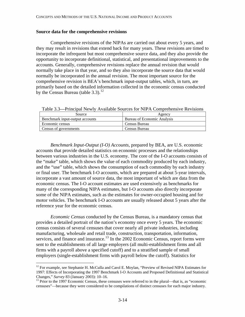
CONCEPTS AND METHODS OF THE U.S. NATIONAL INCOME AND PRODUCT ACCOUNTS
Source data for the comprehensive revisions
Comprehensive revisions of the NIPAs are carried out about every 5 years, and they may result in revisions that extend back for many years. These revisions are timed to incorporate the infrequent but most comprehensive source data, and they also provide the opportunity to incorporate definitional, statistical, and presentational improvements to the accounts. Generally, comprehensive revisions replace the annual revision that would normally take place in that year, and so they also incorporate the source data that would normally be incorporated in the annual revision. The most important source for the comprehensive revision is BEA’s benchmark input-output tables, which, in turn, are primarily based on the detailed information collected in the economic census conducted by the Census Bureau (table 3.3).12
Table 3.3—Principal Newly Available Sources for NIPA Comprehensive Revisions Source Agency
Benchmark input-output accounts Bureau of Economic Analysis Economic census Census Bureau Census of governments Census Bureau
Benchmark Input-Output (I-O) Accounts, prepared by BEA, are U.S. economic accounts that provide detailed statistics on economic processes and the relationships between various industries in the U.S. economy. The core of the I-O accounts consists of the “make” table, which shows the value of each commodity produced by each industry, and the “use” table, which shows the consumption of each commodity by each industry or final user. The benchmark I-O accounts, which are prepared at about 5-year intervals, incorporate a vast amount of source data, the most important of which are data from the economic census. The I-O account estimates are used extensively as benchmarks for many of the corresponding NIPA estimates, but I-O accounts also directly incorporate some of the NIPA estimates, such as the estimates for owner-occupied housing and for motor vehicles. The benchmark I-O accounts are usually released about 5 years after the reference year for the economic census. Economic Census conducted by the Census Bureau, is a mandatory census that provides a detailed portrait of the nation’s economy once every 5 years. The economic census consists of several censuses that cover nearly all private industries, including manufacturing, wholesale and retail trade, construction, transportation, information, services, and finance and insurance.13 In the 2002 Economic Census, report forms were sent to the establishments of all large employers (all multi-establishment firms and all firms with a payroll above a specified cutoff) and to a stratified sample of small employers (single-establishment firms with payroll below the cutoff). Statistics for 12 For example, see Stephanie H. McCulla and Carol E. Moylan, “Preview of Revised NIPA Estimates for 1997: Effects of Incorporating the 1997 Benchmark I-O Accounts and Proposed Definitional and Statistical Changes,” Survey 83 (January 2003): 10–16. 13 Prior to the 1997 Economic Census, these censuses were referred to in the plural—that is, as “economic censuses”—because they were considered to be compilations of distinct censuses for each major industry.
3-14
CONCEPTS AND METHODS OF THE U.S. NATIONAL INCOME AND PRODUCT ACCOUNTS
3-15
selected small employers (for example, those with fewer than 10 employees) and all firms without employees were compiled from administrative records of the IRS and other federal government agencies.14 The economic census is the most important data source for the benchmark I-O accounts. Results from the economic census are released over a period of several years. Census of Governments, which is conducted by the Census Bureau in the same years as the economic census, is a voluntary census that provides periodic and comprehensive statistics about governments and governmental activities. The census covers all state and local governments, including counties, cities, townships, special districts, and school districts. Data are collected on revenues, expenditures, debt, assets, employees, payroll, and benefits for the individual fiscal year that ended prior to July 1 of the census year. These source data are primarily used in estimating state and local government spending. The financial data are released beginning about 16 months after the close of the census year, and the employment data are released beginning about 12 months after the close of the census year.
14 See U.S. Bureau of the Census, Guide to the 2002 Economic Census, at www.census.gov/econ/census02/guide/index.html.
CHAPTER 4: ESTIMATING METHODS Current-Dollar Estimates Adjustments to the source data Seasonal adjustment Moving average Best level and best change Interpolation and extrapolation using an indicator series Three special estimation methods Commodity-flow method Retail control method Perpetual inventory method Quantity and Price Estimates Estimates for detailed components Estimates for NIPA aggregates Properties of chain-type measures Appendix to Chapter 4
Calculating Output and Price Indexes Statistical Tools and Conventions
Chained-dollar measures Contributions to percent change Annual rates Growth rates Rebasing an index The NIPA measures are built up from a wide range of source data using a variety of estimating methods. Each NIPA component is derived using a specific methodology—that is, source data and estimating methods—that progresses from the advance quarterly estimate through the comprehensive NIPA revision. The methodologies used to prepare the various NIPA estimates are periodically changed in order to incorporate improvements in the source data or in the estimating methods.1
• Over time, source data may emerge or disappear, so new source data must be identified and evaluated, and estimating methods must be adapted accordingly.
• Advances in statistical techniques or in other aspects of estimation must be evaluated for adoption into the methodology.
• As the U.S. economy evolves, the methodology must be updated to ensure that the estimates continue to provide a reliable and relevant picture of transactions and transactors in the economy.
1 Substantive changes to NIPA methodologies are documented in BEA’s monthly Survey of Current Business.
4-1
CONCEPTS AND METHODS OF THE U.S. NATIONAL INCOME AND PRODUCT ACCOUNTS
The examples provided in this chapter are simplified in order to illustrate the basic estimating concepts and calculations. In practice, the procedures used for deriving the NIPAs involve complex statistical techniques that are designed to ensure consistency across the entire time series for a given estimate and between interrelated estimates.
Current-Dollar Estimates For most NIPA components, the current-dollar, or nominal, estimates are derived from source data that are “value data,” which reflect the product of quantity and price. For the estimates that are not derived from value data, separate quantity data and price data must be combined. For example, an estimate of expenditures on new autos may be calculated as the number of autos sold times expenditure per auto (at transaction prices—that is, the average list price with options adjusted for transportation charges, sales taxes, dealer discounts, and rebates). An estimate of wages may be calculated as employment times average hourly earnings times average hours worked, and an estimate of interest received may be calculated as the stock of interest-bearing assets times an effective interest rate. (The NIPA current-dollar estimates are expressed at annual rates; see the appendix to this chapter.) Adjustments to the source data
BEA makes three general types of adjustments to the source data that are incorporated into the NIPA estimates. The first consists of adjustments that are needed so that the data conform to appropriate NIPA concepts and definitions. For example, Internal Revenue Service data from corporate tax returns include estimates of depreciation, but these estimates are based on historical-cost valuation and on tax service lives. BEA must adjust these estimates to the NIPA definition of depreciation—consumption of fixed capital—which is based on current-cost valuation and economic service lives.
The second type of adjustment involves filling gaps in coverage. For example,
one of the primary sources for the quarterly estimates of the change in private inventories component of GDP is the Census Bureau’s monthly survey of wholesale trade. However, this source does not cover inventories of nonmerchant wholesalers (wholesalers that do not take title to the goods they sell). Thus, the survey data must be augmented by separate BEA estimates for the change in the inventories of these wholesalers.
The third type of adjustment involves time of recording and valuation. For
example, in the NIPAs (as in BEA’s international transactions accounts), imported goods are valued at “foreign port value”—that is, the value at the point of exportation to the United States. The source data on imports of goods from Canada, which the Census Bureau receives in a bilateral data exchange with Canada, are often valued at the point of manufacture; thus, BEA must adjust these data to foreign port value by adding the cost of transporting these goods within Canada from the point of manufacture to the point of export to the United States.
4-2
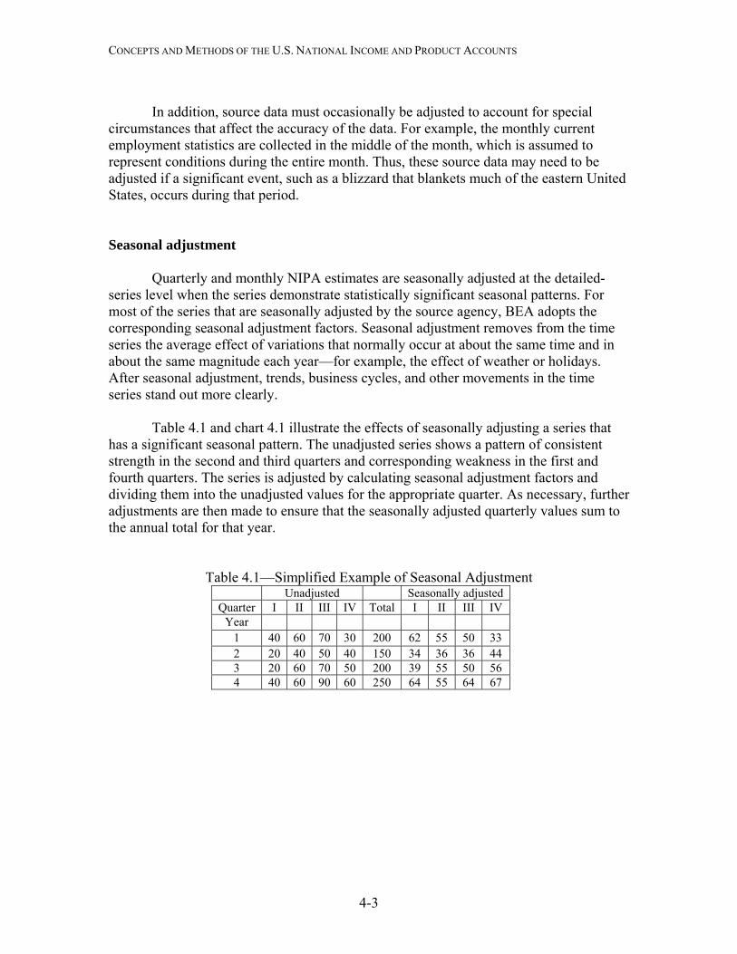
CONCEPTS AND METHODS OF THE U.S. NATIONAL INCOME AND PRODUCT ACCOUNTS
In addition, source data must occasionally be adjusted to account for special circumstances that affect the accuracy of the data. For example, the monthly current employment statistics are collected in the middle of the month, which is assumed to represent conditions during the entire month. Thus, these source data may need to be adjusted if a significant event, such as a blizzard that blankets much of the eastern United States, occurs during that period. Seasonal adjustment
Quarterly and monthly NIPA estimates are seasonally adjusted at the detailed-series level when the series demonstrate statistically significant seasonal patterns. For most of the series that are seasonally adjusted by the source agency, BEA adopts the corresponding seasonal adjustment factors. Seasonal adjustment removes from the time series the average effect of variations that normally occur at about the same time and in about the same magnitude each year—for example, the effect of weather or holidays. After seasonal adjustment, trends, business cycles, and other movements in the time series stand out more clearly. Table 4.1 and chart 4.1 illustrate the effects of seasonally adjusting a series that has a significant seasonal pattern. The unadjusted series shows a pattern of consistent strength in the second and third quarters and corresponding weakness in the first and fourth quarters. The series is adjusted by calculating seasonal adjustment factors and dividing them into the unadjusted values for the appropriate quarter. As necessary, further adjustments are then made to ensure that the seasonally adjusted quarterly values sum to the annual total for that year.
Table 4.1—Simplified Example of Seasonal Adjustment
Unadjusted Seasonally adjusted Quarter I II III IV Total I II III IV
Year 1 40 60 70 30 200 62 55 50 33 2 20 40 50 40 150 34 36 36 44 3 20 60 70 50 200 39 55 50 56 4 40 60 90 60 250 64 55 64 67
4-3
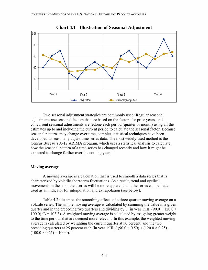
CONCEPTS AND METHODS OF THE U.S. NATIONAL INCOME AND PRODUCT ACCOUNTS
Chart 4.1—Illustration of Seasonal Adjustment
Two seasonal adjustment strategies are commonly used: Regular seasonal adjustments use seasonal factors that are based on the factors for prior years, and concurrent seasonal adjustments are redone each period (quarter or month) using all the estimates up to and including the current period to calculate the seasonal factor. Because seasonal patterns may change over time, complex statistical techniques have been developed to seasonally adjust time series data. The most widely used method is the Census Bureau’s X-12 ARIMA program, which uses a statistical analysis to calculate how the seasonal pattern of a time series has changed recently and how it might be expected to change further over the coming year. Moving average A moving average is a calculation that is used to smooth a data series that is characterized by volatile short-term fluctuations. As a result, trend and cyclical movements in the smoothed series will be more apparent, and the series can be better used as an indicator for interpolation and extrapolation (see below). Table 4.2 illustrates the smoothing effects of a three-quarter moving average on a volatile series. The simple moving average is calculated by summing the value in a given quarter and in the preceding two quarters and dividing by 3 (in year 1:III, (90.0 + 120.0 + 100.0) ⁄ 3 = 103.3). A weighted moving average is calculated by assigning greater weight to the time periods that are deemed more relevant. In this example, the weighted moving average is calculated by weighting the current quarter at 50 percent, and the two preceding quarters at 25 percent each (in year 1:III, ( (90.0 × 0.50) + (120.0 × 0.25) + (100.0 × 0.25) = 100.0).
4-4
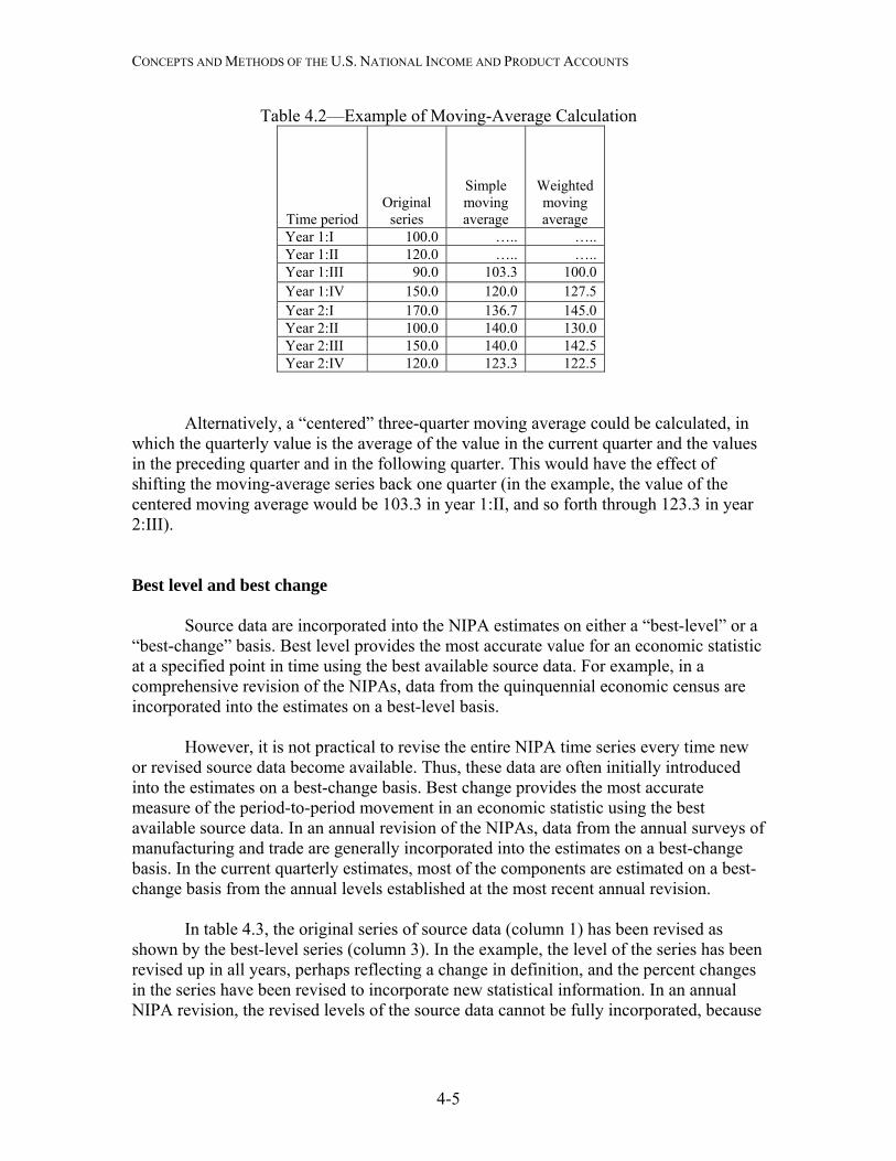
CONCEPTS AND METHODS OF THE U.S. NATIONAL INCOME AND PRODUCT ACCOUNTS
Table 4.2—Example of Moving-Average Calculation
Time period Original
series
Simple moving average
Weighted moving average
Year 1:I 100.0 ….. ….. Year 1:II 120.0 ….. ….. Year 1:III 90.0 103.3 100.0 Year 1:IV 150.0 120.0 127.5 Year 2:I 170.0 136.7 145.0 Year 2:II 100.0 140.0 130.0 Year 2:III 150.0 140.0 142.5 Year 2:IV 120.0 123.3 122.5
Alternatively, a “centered” three-quarter moving average could be calculated, in which the quarterly value is the average of the value in the current quarter and the values in the preceding quarter and in the following quarter. This would have the effect of shifting the moving-average series back one quarter (in the example, the value of the centered moving average would be 103.3 in year 1:II, and so forth through 123.3 in year 2:III). Best level and best change Source data are incorporated into the NIPA estimates on either a “best-level” or a “best-change” basis. Best level provides the most accurate value for an economic statistic at a specified point in time using the best available source data. For example, in a comprehensive revision of the NIPAs, data from the quinquennial economic census are incorporated into the estimates on a best-level basis.
However, it is not practical to revise the entire NIPA time series every time new or revised source data become available. Thus, these data are often initially introduced into the estimates on a best-change basis. Best change provides the most accurate measure of the period-to-period movement in an economic statistic using the best available source data. In an annual revision of the NIPAs, data from the annual surveys of manufacturing and trade are generally incorporated into the estimates on a best-change basis. In the current quarterly estimates, most of the components are estimated on a best-change basis from the annual levels established at the most recent annual revision. In table 4.3, the original series of source data (column 1) has been revised as shown by the best-level series (column 3). In the example, the level of the series has been revised up in all years, perhaps reflecting a change in definition, and the percent changes in the series have been revised to incorporate new statistical information. In an annual NIPA revision, the revised levels of the source data cannot be fully incorporated, because
4-5

CONCEPTS AND METHODS OF THE U.S. NATIONAL INCOME AND PRODUCT ACCOUNTS
annual revisions only cover the 3 most recent years.2 As can be seen in this example, incorporating the revised best-level series only for years 2–4 would result in a discontinuity between the unrevised estimate for year 1 (100.0) and the revised estimate for year 2 (115.0) (a 15.0-percent increase rather than the 10.6-percent increase indicated by the source data). To avoid this problem, the revised source data are instead incorporated on a best-change basis—that is, a new best-change series is created by beginning with the value in the unrevised year 1 (100.0) and applying the percent changes in the best-level series (column 4). As a result, the level of the new series (column 5) is kept consistent with the level of the earlier nonrevised year, while the percent changes in the new series (column 6) fully reflect the new statistical information that was incorporated into the source data. In the next comprehensive revision, the revised best-levels would be incorporated into the NIPA estimates.
Table 4.3—Simplified Example of “Best Level” and “Best Change”
Year
Original series
[billions of dollars ]
(1)
Percent change in original series
(2)
Revised (“best-level”) series
[billions of dollars]
(3)
Percent change in best-level
series
(4)
Revised (“best-
change”) series
[billions of dollars]
(5)
Percent change in
best-change series
(6)
1 100.0 .…. 104.0 ….. 100.0 ….. 2 110.0 10.0 115.0 10.6 110.6 10.6 3 120.0 9.1 124.0 7.8 119.2 7.8 4 130.0 8.3 136.0 9.7 130.8 9.7
Interpolation and extrapolation using an indicator series Generally, monthly or quarterly source data are not as comprehensive or as reliable as annual source data (and, similarly, annual source data are not as comprehensive or as reliable as quinquennial source data). Thus, for some estimates, the more frequent but less comprehensive source data may be used as an indicator of the movements of the component series rather than as a measure of the absolute levels of the series. Specifically, for the periods for which annual estimates are available and the quarterly estimates must be forced to average to these annual totals, the quarterly pattern is estimated by interpolation. For the periods not yet covered by annual estimates (such as the current quarter), the quarterly estimates are made by extrapolation. The use of an indicator series to estimate a component is illustrated in table 4.4. We begin with a value of $200 (annual rate) for the fourth quarter of year 1 (this value 2 Starting in 2010, BEA adopted a flexible approach to annual revisions that allows improvements in concepts, definitions, and source data to be introduced and that allows the expansion of the 3-year revision period to earlier periods if necessary; see “BEA Briefing: Improving BEA’s Accounts Through Flexible Annual Revisions,” Survey 88 (June 2008): 29–32.
4-6
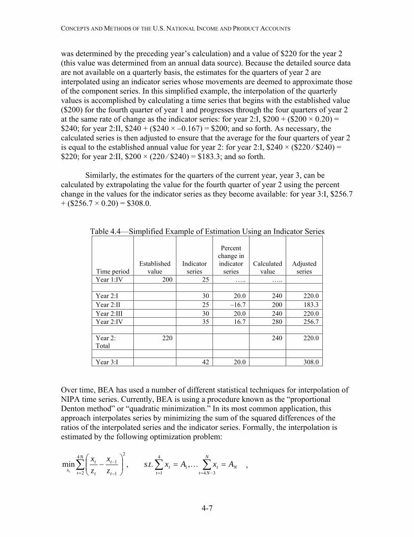
CONCEPTS AND METHODS OF THE U.S. NATIONAL INCOME AND PRODUCT ACCOUNTS
was determined by the preceding year’s calculation) and a value of $220 for the year 2 (this value was determined from an annual data source). Because the detailed source data are not available on a quarterly basis, the estimates for the quarters of year 2 are interpolated using an indicator series whose movements are deemed to approximate those of the component series. In this simplified example, the interpolation of the quarterly values is accomplished by calculating a time series that begins with the established value ($200) for the fourth quarter of year 1 and progresses through the four quarters of year 2 at the same rate of change as the indicator series: for year 2:I, $200 + ($200 × 0.20) = $240; for year 2:II, $240 + ($240 × –0.167) = $200; and so forth. As necessary, the calculated series is then adjusted to ensure that the average for the four quarters of year 2 is equal to the established annual value for year 2: for year 2:I, $240 × ($220 ⁄ $240) = $220; for year 2:II, $200 × (220 ⁄ $240) = $183.3; and so forth.
Similarly, the estimates for the quarters of the current year, year 3, can be
calculated by extrapolating the value for the fourth quarter of year 2 using the percent change in the values for the indicator series as they become available: for year 3:I, $256.7 + ($256.7 × 0.20) = $308.0.
Table 4.4—Simplified Example of Estimation Using an Indicator Series
Time period Established
value
Indicator series
Percent change in indicator
series
Calculated value
Adjusted series
Year 1:IV 200 25 ….. ….. Year 2:I 30 20.0 240 220.0 Year 2:II 25 –16.7 200 183.3 Year 2:III 30 20.0 240 220.0 Year 2:IV 35 16.7 280 256.7 Year 2: Total
220 240 220.0
Year 3:I 42 20.0 308.0
Over time, BEA has used a number of different statistical techniques for interpolation of NIPA time series. Currently, BEA is using a procedure known as the “proportional Denton method” or “quadratic minimization.” In its most common application, this approach interpolates series by minimizing the sum of the squared differences of the ratios of the interpolated series and the indicator series. Formally, the interpolation is estimated by the following optimization problem:
,
∑∑∑−=== −
− ==⎟⎟⎠
⎞⎜⎜⎝
⎛−
N
NtNt
tt
N
t t
t
t
t
xAxAxts
zx
zx
t 34
4
11
4
2
2
1
1 ,..,min K
4-7
CONCEPTS AND METHODS OF THE U.S. NATIONAL INCOME AND PRODUCT ACCOUNTS
where z is the indicator series, x is the interpolated series, A are the annual controls that the interpolated series must sum to, and N is the number of years for the interpolation. This example shows an annual-to-quarterly interpolation. The same method can also be used for annual-to-monthly and quarterly-to-monthly interpolation.3 Three special estimation methods In certain cases where primary source data are not available, one or more of the following special methods—commodity flow, retail control, or perpetual inventory—may be used to estimate values. Commodity-flow method
The commodity-flow method is generally used to derive estimates in economic census years for various components of consumer spending, equipment and software, and the commodity detail for state and local government consumption expenditures and gross investment. An abbreviated form of this method is used to prepare estimates of investment in equipment in nonbenchmark years, and an even more abbreviated form is used to prepare the current quarterly estimates of investment in equipment.
The commodity-flow method begins with estimates of the domestic output or domestic sales of a commodity valued in producers’ prices.4 Then, estimates of the domestic supply of that commodity—the amount that is available for domestic consumption—are prepared by adding imports and by subtracting exports and inventory change. Next, the domestic supply of the commodity is allocated among domestic purchasers—that is, persons, business, and government. Finally, the estimates are converted to purchasers’ prices.5 The commodity-flow method is illustrated in table 4.5. First, domestic shipments—the value of shipments of the commodity produced by domestic firms at producers’ prices—are converted to net supply, by adding imports and subtracting exports, government purchases, and change in inventories (a positive change in inventories reduces net supply and a negative change in inventories raises net supply) (in the example, $100 + $40 – $10 – $5 – $5 = $120). Portions of the net supply are then allocated among business intermediate purchases and consumer spending. This allocation may be based on relationships from the most recent economic census or on information from other sources (such as spending by consumers as determined by the retail control method). In this example, it is assumed that one-fourth of net supply is allocated to 3 See Baoline Chen and Stephen H. Andrews, “An Empirical Review of Methods for Temporal Distribution and Interpolation in the National Accounts,” Survey 88 (May 2008): 31–37. 4 Producers’ prices are the prices received by producers for the goods and services they sell. These prices include sales and excise taxes but exclude domestic transportation costs and trade margins. Trade margins, or markups, reflect the value added by wholesalers and retailers in the distribution of a commodity from producers to final purchasers. 5 Purchasers’ prices are the prices paid by intermediate and final purchasers for the goods and services they buy. These prices are equal to producers’ prices plus domestic transportation costs and trade margins.
4-8
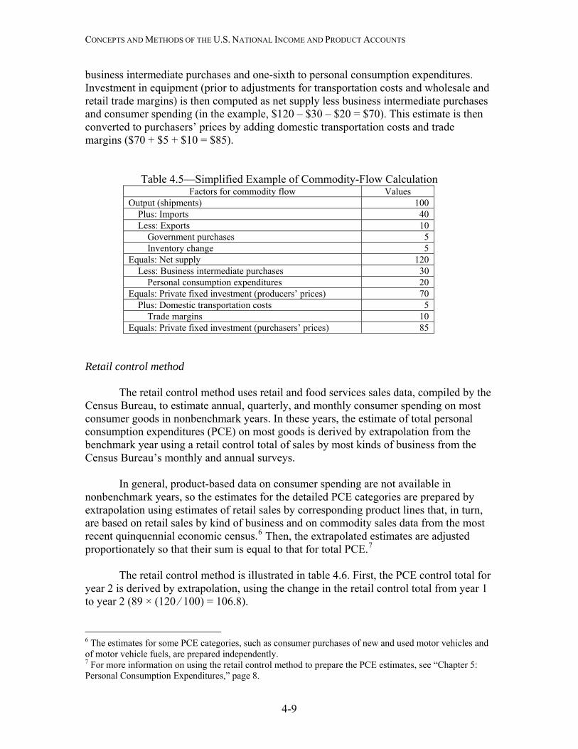
CONCEPTS AND METHODS OF THE U.S. NATIONAL INCOME AND PRODUCT ACCOUNTS
business intermediate purchases and one-sixth to personal consumption expenditures. Investment in equipment (prior to adjustments for transportation costs and wholesale and retail trade margins) is then computed as net supply less business intermediate purchases and consumer spending (in the example, $120 – $30 – $20 = $70). This estimate is then converted to purchasers’ prices by adding domestic transportation costs and trade margins ($70 + $5 + $10 = $85).
Table 4.5—Simplified Example of Commodity-Flow Calculation Factors for commodity flow Values
Output (shipments) 100 Plus: Imports 40 Less: Exports 10 Government purchases 5 Inventory change 5 Equals: Net supply 120 Less: Business intermediate purchases 30 Personal consumption expenditures 20 Equals: Private fixed investment (producers’ prices) 70 Plus: Domestic transportation costs 5 Trade margins 10 Equals: Private fixed investment (purchasers’ prices) 85
Retail control method
The retail control method uses retail and food services sales data, compiled by the
Census Bureau, to estimate annual, quarterly, and monthly consumer spending on most consumer goods in nonbenchmark years. In these years, the estimate of total personal consumption expenditures (PCE) on most goods is derived by extrapolation from the benchmark year using a retail control total of sales by most kinds of business from the Census Bureau’s monthly and annual surveys.
In general, product-based data on consumer spending are not available in
nonbenchmark years, so the estimates for the detailed PCE categories are prepared by extrapolation using estimates of retail sales by corresponding product lines that, in turn, are based on retail sales by kind of business and on commodity sales data from the most recent quinquennial economic census.6 Then, the extrapolated estimates are adjusted proportionately so that their sum is equal to that for total PCE.7
The retail control method is illustrated in table 4.6. First, the PCE control total for
year 2 is derived by extrapolation, using the change in the retail control total from year 1 to year 2 (89 × (120 ⁄ 100) = 106.8).
6 The estimates for some PCE categories, such as consumer purchases of new and used motor vehicles and of motor vehicle fuels, are prepared independently. 7 For more information on using the retail control method to prepare the PCE estimates, see “Chapter 5: Personal Consumption Expenditures,” page 8.
4-9
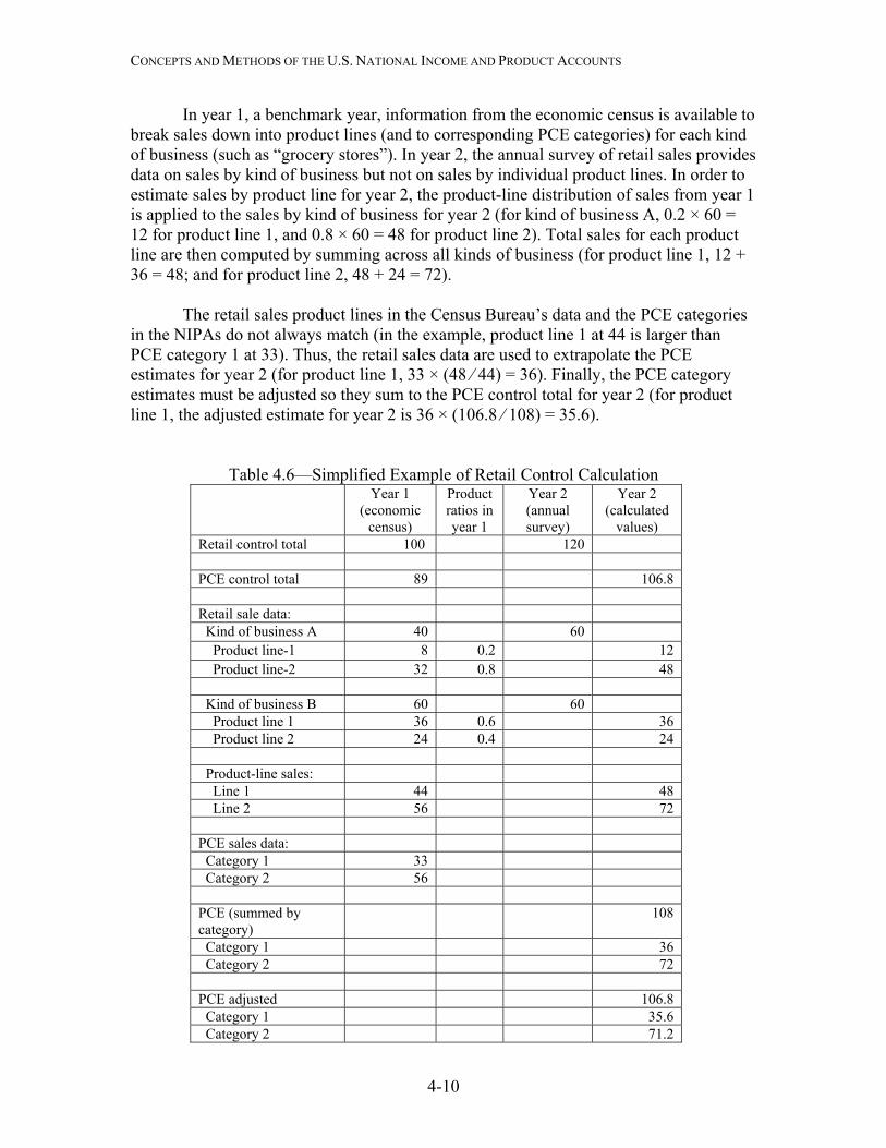
CONCEPTS AND METHODS OF THE U.S. NATIONAL INCOME AND PRODUCT ACCOUNTS
In year 1, a benchmark year, information from the economic census is available to break sales down into product lines (and to corresponding PCE categories) for each kind of business (such as “grocery stores”). In year 2, the annual survey of retail sales provides data on sales by kind of business but not on sales by individual product lines. In order to estimate sales by product line for year 2, the product-line distribution of sales from year 1 is applied to the sales by kind of business for year 2 (for kind of business A, 0.2 × 60 = 12 for product line 1, and 0.8 × 60 = 48 for product line 2). Total sales for each product line are then computed by summing across all kinds of business (for product line 1, 12 + 36 = 48; and for product line 2, 48 + 24 = 72).
The retail sales product lines in the Census Bureau’s data and the PCE categories
in the NIPAs do not always match (in the example, product line 1 at 44 is larger than PCE category 1 at 33). Thus, the retail sales data are used to extrapolate the PCE estimates for year 2 (for product line 1, 33 × (48 ⁄ 44) = 36). Finally, the PCE category estimates must be adjusted so they sum to the PCE control total for year 2 (for product line 1, the adjusted estimate for year 2 is 36 × (106.8 ⁄ 108) = 35.6).
Table 4.6—Simplified Example of Retail Control Calculation
Year 1 (economic
census)
Product ratios in year 1
Year 2 (annual survey)
Year 2 (calculated
values) Retail control total 100 120 PCE control total 89 106.8 Retail sale data: Kind of business A 40 60 Product line-1 8 0.2 12 Product line-2 32 0.8 48 Kind of business B 60 60 Product line 1 36 0.6 36 Product line 2 24 0.4 24 Product-line sales: Line 1 44 48 Line 2 56 72 PCE sales data: Category 1 33 Category 2 56 PCE (summed by category)
108
Category 1 36 Category 2 72 PCE adjusted 106.8 Category 1 35.6 Category 2 71.2
4-10
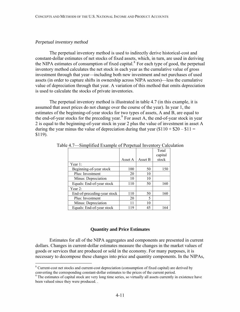
CONCEPTS AND METHODS OF THE U.S. NATIONAL INCOME AND PRODUCT ACCOUNTS
Perpetual inventory method
The perpetual inventory method is used to indirectly derive historical-cost and constant-dollar estimates of net stocks of fixed assets, which, in turn, are used in deriving the NIPA estimates of consumption of fixed capital.8 For each type of good, the perpetual inventory method calculates the net stock in each year as the cumulative value of gross investment through that year—including both new investment and net purchases of used assets (in order to capture shifts in ownership across NIPA sectors)—less the cumulative value of depreciation through that year. A variation of this method that omits depreciation is used to calculate the stocks of private inventories. The perpetual inventory method is illustrated in table 4.7 (in this example, it is assumed that asset prices do not change over the course of the year). In year 1, the estimates of the beginning-of-year stocks for two types of assets, A and B, are equal to the end-of-year stocks for the preceding year.9 For asset A, the end-of-year stock in year 2 is equal to the beginning-of-year stock in year 2 plus the value of investment in asset A during the year minus the value of depreciation during that year ($110 + $20 – $11 = $119).
Table 4.7—Simplified Example of Perpetual Inventory Calculation
Asset A Asset B
Total capital stock
Year 1: Beginning-of-year stock 100 50 150 Plus: Investment 20 10 Minus: Depreciation 10 10 Equals: End-of-year stock 110 50 160 Year 2: End-of-preceding-year stock 110 50 160 Plus: Investment 20 5 Minus: Depreciation 11 10 Equals: End-of-year stock 119 45 164
Quantity and Price Estimates Estimates for all of the NIPA aggregates and components are presented in current dollars. Changes in current-dollar estimates measure the changes in the market values of goods or services that are produced or sold in the economy. For many purposes, it is necessary to decompose these changes into price and quantity components. In the NIPAs, 8 Current-cost net stocks and current-cost depreciation (consumption of fixed capital) are derived by converting the corresponding constant-dollar estimates to the prices of the current period. 9 The estimates of capital stock are very long time series, so virtually all assets currently in existence have been valued since they were produced. .
4-11
CONCEPTS AND METHODS OF THE U.S. NATIONAL INCOME AND PRODUCT ACCOUNTS
prices and quantities are expressed as index numbers with the reference year—at present, the year 2005—equal to 100. For selected series, quantities—or “real” (inflation adjusted) measures—are also expressed in chained (2005) dollars. (Period-to-period changes in quantities and prices are expressed as percent changes at annual rates; see “Statistical Tools and Conventions” in the appendix to this chapter.)
BEA prepares quantity estimates for GDP and its product-side components and
for a few other aggregates and components. (For an illustration of the calculation of these estimates from a set of quantity and price information, see “Calculation of Output and Price Indexes” in the appendix to this chapter.) Estimates for detailed components
For the detailed NIPA components, the quantity estimates are prepared using one of three methods—deflation, quantity extrapolation, or direct valuation—depending on the availability of source data. The quantity estimates are expressed as real values with 2005 (at present) as the reference year.
Deflation. Because the source data available for most components of GDP are
measured in dollars rather than in units, the quantities of most of the detailed components are obtained by deflation. For deflation, quantities are calculated by dividing the current-dollar value of the component by an “appropriate” price index (with the reference-year value set to 100).10
Qt = (ptqt)⁄(pt⁄po), where pt and qt are observed prices and quantities in the current year and po is the observed price in the reference year.
Thus, for example, if the current-dollar value for the component series is $14 in 2006 and the appropriate price index is 112 in 2006, then the quantity estimate for the component series in 2006 is ($14 ⁄ (112 ⁄ 100)), or $12.50.
Quantity extrapolation. The other two methods are similar in that they both are derived using quantity data. Quantity extrapolation is used when a quantity indicator series is available that approximates the movements of the component series. In this method, the quantity estimate is obtained by using the indicator series to extrapolate from the reference-year value. Qt = poqo+((poqo)×((qt′ –qo′)⁄qo′)), where q′ represents the quantity indicator series. For example, if the dollar value of the component series is $10 in 2005 and the quantity indicator series shows an increase of 25 percent in 2006, then the quantity estimate for the component series in 2006 is ($10 + ($10 × 25/100)), or $12.50. 10 A price index is appropriate if its definition and coverage closely match those of the series being deflated.
4-12
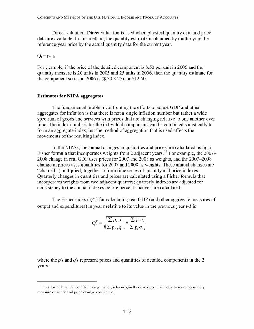
CONCEPTS AND METHODS OF THE U.S. NATIONAL INCOME AND PRODUCT ACCOUNTS
Direct valuation. Direct valuation is used when physical quantity data and price data are available. In this method, the quantity estimate is obtained by multiplying the reference-year price by the actual quantity data for the current year. Qt = poqt. For example, if the price of the detailed component is $.50 per unit in 2005 and the quantity measure is 20 units in 2005 and 25 units in 2006, then the quantity estimate for the component series in 2006 is ($.50 × 25), or $12.50. Estimates for NIPA aggregates The fundamental problem confronting the efforts to adjust GDP and other aggregates for inflation is that there is not a single inflation number but rather a wide spectrum of goods and services with prices that are changing relative to one another over time. The index numbers for the individual components can be combined statistically to form an aggregate index, but the method of aggregation that is used affects the movements of the resulting index. In the NIPAs, the annual changes in quantities and prices are calculated using a Fisher formula that incorporates weights from 2 adjacent years.11 For example, the 2007–2008 change in real GDP uses prices for 2007 and 2008 as weights, and the 2007–2008 change in prices uses quantities for 2007 and 2008 as weights. These annual changes are “chained” (multiplied) together to form time series of quantity and price indexes. Quarterly changes in quantities and prices are calculated using a Fisher formula that incorporates weights from two adjacent quarters; quarterly indexes are adjusted for consistency to the annual indexes before percent changes are calculated. The Fisher index ( ) for calculating real GDP (and other aggregate measures of output and expenditures) in year t relative to its value in the previous year t-1 is
FtQ
,qpqp
qpqp
=Q1-tt
tt
1-t1-t
t1-tFt ∑
∑×
∑∑
where the p's and q's represent prices and quantities of detailed components in the 2 years.
11 This formula is named after Irving Fisher, who originally developed this index to more accurately measure quantity and price changes over time.
4-13
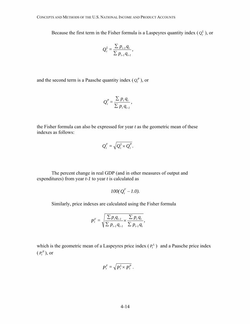
CONCEPTS AND METHODS OF THE U.S. NATIONAL INCOME AND PRODUCT ACCOUNTS
Because the first term in the Fisher formula is a Laspeyres quantity index ( ), or QLt
,qpqp=Q
1-t1-t
t1-tLt ∑
∑
and the second term is a Paasche quantity index ( ), or P
tQ
,qpqp
=Q1-tt
ttPt ∑
∑
the Fisher formula can also be expressed for year t as the geometric mean of these indexes as follows:
.QQ=Q Pt
Lt
Ft ×
The percent change in real GDP (and in other measures of output and expenditures) from year t-1 to year t is calculated as
1.0).Q100( Ft –
Similarly, price indexes are calculated using the Fisher formula
,qpqp
qpqp
=Pt1-t
tt
1-t1-t
1-ttFt ∑
∑×
∑∑
which is the geometric mean of a Laspeyres price index ( ) and a Paasche price index ( ), or
LtP
PtP
PP=P Pt
Lt
Ft × .
4-14
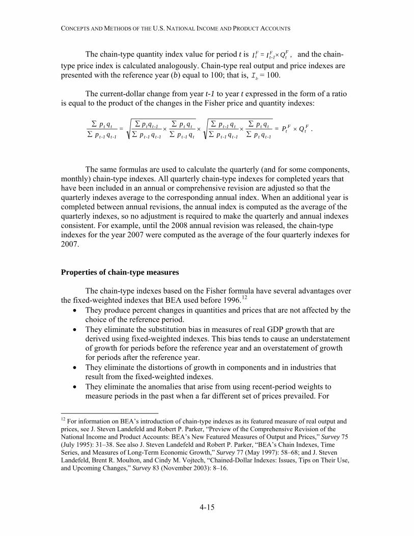
CONCEPTS AND METHODS OF THE U.S. NATIONAL INCOME AND PRODUCT ACCOUNTS
The chain-type quantity index value for period t is and the chain-type price index is calculated analogously. Chain-type real output and price indexes are presented with the reference year (b) equal to 100; that is, Ib = 100.
,QI=I Ft
F1-t
Ft ×
The current-dollar change from year t-1 to year t expressed in the form of a ratio
is equal to the product of the changes in the Fisher price and quantity indexes:
Ft
Ft
-1tt
tt
-1t-1t
t-1t
t-1t
tt
-1t-1t
-1tt
-1t-1t
tt QP=qpqp
qpqp
qpqp
qpqp
=qpqp
×∑∑
×∑∑
×∑∑
×∑∑
∑∑ .
The same formulas are used to calculate the quarterly (and for some components, monthly) chain-type indexes. All quarterly chain-type indexes for completed years that have been included in an annual or comprehensive revision are adjusted so that the quarterly indexes average to the corresponding annual index. When an additional year is completed between annual revisions, the annual index is computed as the average of the quarterly indexes, so no adjustment is required to make the quarterly and annual indexes consistent. For example, until the 2008 annual revision was released, the chain-type indexes for the year 2007 were computed as the average of the four quarterly indexes for 2007. Properties of chain-type measures The chain-type indexes based on the Fisher formula have several advantages over the fixed-weighted indexes that BEA used before 1996.12
• They produce percent changes in quantities and prices that are not affected by the choice of the reference period.
• They eliminate the substitution bias in measures of real GDP growth that are derived using fixed-weighted indexes. This bias tends to cause an understatement of growth for periods before the reference year and an overstatement of growth for periods after the reference year.
• They eliminate the distortions of growth in components and in industries that result from the fixed-weighted indexes.
• They eliminate the anomalies that arise from using recent-period weights to measure periods in the past when a far different set of prices prevailed. For
12 For information on BEA’s introduction of chain-type indexes as its featured measure of real output and prices, see J. Steven Landefeld and Robert P. Parker, “Preview of the Comprehensive Revision of the National Income and Product Accounts: BEA’s New Featured Measures of Output and Prices,” Survey 75 (July 1995): 31–38. See also J. Steven Landefeld and Robert P. Parker, “BEA’s Chain Indexes, Time Series, and Measures of Long-Term Economic Growth,” Survey 77 (May 1997): 58–68; and J. Steven Landefeld, Brent R. Moulton, and Cindy M. Vojtech, “Chained-Dollar Indexes: Issues, Tips on Their Use, and Upcoming Changes,” Survey 83 (November 2003): 8–16.
4-15
CONCEPTS AND METHODS OF THE U.S. NATIONAL INCOME AND PRODUCT ACCOUNTS
example, the prices of defense equipment in the 2000s are not appropriate for measuring the real changes in defense spending in the 1940s.
• They eliminate the inconvenience and confusion associated with BEA’s previous practice of updating weights and years—and thereby rewriting economic history—about every 5 years.
Despite the greater accuracy provided by the chain-type indexes, users of
macroeconomic statistics need more than index numbers and percent changes. The earlier fixed-weighted estimates were denominated in constant dollars, and the real levels for the components of GDP added up to total GDP. Because the system was additive, the shares of the real components reflected their relative importance in total GDP. Similarly, in decomposing total GDP growth by component, the change in constant-dollar values measured the component’s contribution to the change in the fixed-weighted aggregate. For GDP and most of its components, BEA prepares estimates in chained dollars as well as chain-type indexes (see the appendix to this chapter). However, because these chained-dollar measures are not based on a single set of weights, they are not additive and thus do not yield accurate measures of shares and contributions to growth.
For real GDP and its major components, BEA provides tables that present accurate estimates of contributions to growth rates that are based on chain-type quantity indexes rather than on the chained-dollar estimates (see the appendix). In addition, BEA provides measures of percentage shares that are based on current-dollar values. Because current-dollar values provide the weights for the chain-type indexes, shares calculated from these estimates rather than from the chained-dollar estimates should be used to indicate the relative importance of components
4-16
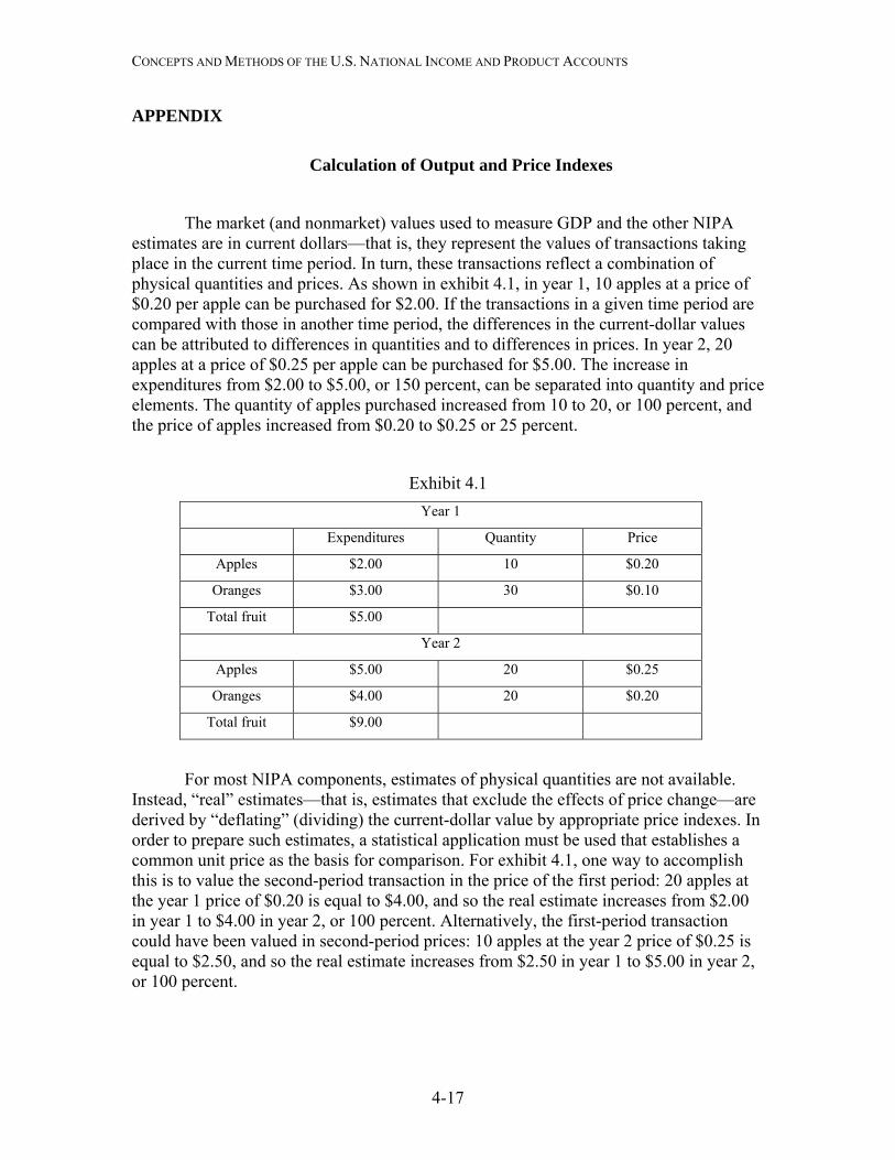
CONCEPTS AND METHODS OF THE U.S. NATIONAL INCOME AND PRODUCT ACCOUNTS
APPENDIX
Calculation of Output and Price Indexes
The market (and nonmarket) values used to measure GDP and the other NIPA estimates are in current dollars—that is, they represent the values of transactions taking place in the current time period. In turn, these transactions reflect a combination of physical quantities and prices. As shown in exhibit 4.1, in year 1, 10 apples at a price of $0.20 per apple can be purchased for $2.00. If the transactions in a given time period are compared with those in another time period, the differences in the current-dollar values can be attributed to differences in quantities and to differences in prices. In year 2, 20 apples at a price of $0.25 per apple can be purchased for $5.00. The increase in expenditures from $2.00 to $5.00, or 150 percent, can be separated into quantity and price elements. The quantity of apples purchased increased from 10 to 20, or 100 percent, and the price of apples increased from $0.20 to $0.25 or 25 percent.
Exhibit 4.1 Year 1
Expenditures Quantity Price
Apples $2.00 10 $0.20
Oranges $3.00 30 $0.10
Total fruit $5.00
Year 2
Apples $5.00 20 $0.25
Oranges $4.00 20 $0.20
Total fruit $9.00
For most NIPA components, estimates of physical quantities are not available. Instead, “real” estimates—that is, estimates that exclude the effects of price change—are derived by “deflating” (dividing) the current-dollar value by appropriate price indexes. In order to prepare such estimates, a statistical application must be used that establishes a common unit price as the basis for comparison. For exhibit 4.1, one way to accomplish this is to value the second-period transaction in the price of the first period: 20 apples at the year 1 price of $0.20 is equal to $4.00, and so the real estimate increases from $2.00 in year 1 to $4.00 in year 2, or 100 percent. Alternatively, the first-period transaction could have been valued in second-period prices: 10 apples at the year 2 price of $0.25 is equal to $2.50, and so the real estimate increases from $2.50 in year 1 to $5.00 in year 2, or 100 percent.
4-17
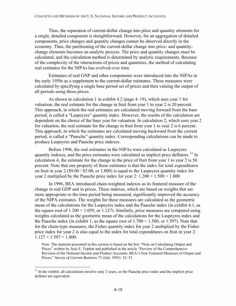
CONCEPTS AND METHODS OF THE U.S. NATIONAL INCOME AND PRODUCT ACCOUNTS
Thus, the separation of current-dollar change into price and quantity elements for a single, detailed component is straightforward. However, for an aggregation of detailed components, price changes and quantity changes cannot be observed directly in the economy. Thus, the partitioning of the current-dollar change into price- and quantity-change elements becomes an analytic process. The price and quantity changes must be calculated, and the calculation method is determined by analytic requirements. Because of the complexity of the interactions of prices and quantities, the method of calculating real estimates for the NIPAs has evolved over time.
Estimates of real GNP and other components were introduced into the NIPAs in the early 1950s as a supplement to the current-dollar estimates. These measures were calculated by specifying a single base period set of prices and then valuing the output of all periods using those prices.
As shown in calculation 1 in exhibit 4.2 (page 4–19), which uses year 1 for valuation, the real estimate for the change in fruit from year 1 to year 2 is 20 percent. This approach, in which the real estimates are calculated moving forward from the base period, is called a “Laspeyres” quantity index. However, the results of the calculation are dependent on the choice of the base year for valuation. In calculation 2, which uses year 2 for valuation, the real estimate for the change in fruit from year 1 to year 2 is 6 percent. This approach, in which the estimates are calculated moving backward from the current period, is called a “Paasche” quantity index. Corresponding calculations can be made to produce Laspeyres and Paasche price indexes.
Before 1996, the real estimates in the NIPAs were calculated as Laspeyres quantity indexes, and the price estimates were calculated as implicit price deflators.13 In calculation 4, the estimate for the change in the price of fruit from year 1 to year 2 is 50 percent. Note that one property of these estimates is that the index for total expenditures on fruit in year 2 ($9.00 / $5.00, or 1.800) is equal to the Laspeyres quantity index for year 2 multiplied by the Paasche price index for year 2: 1.200 × 1.500 = 1.800
In 1996, BEA introduced chain-weighted indexes as its featured measure of the change in real GDP and in prices. These indexes, which are based on weights that are more appropriate to the time period being measured, significantly improved the accuracy of the NIPA estimates. The weights for these measures are calculated as the geometric mean of the calculations for the Laspeyres index and the Paasche index (in exhibit 4.1, as the square root of 1.200 × 1.059, or 1.127). Similarly, price measures are computed using weights calculated as the geometric mean of the calculations for the Laspeyres index and the Paasche index (in exhibit 1, as the square root of 1.700 × 1.500, or 1.597). Note that for the chain-type measures, the Fisher quantity index for year 2 multiplied by the Fisher price index for year 2 is also equal to the index for total expenditures on fruit in year 2: 1.127 × 1.597 = 1.800.
Note. The material presented in this section is based on the box “Note on Calculating Output and Prices” written by Jack E. Triplett and published in the article “Preview of the Comprehensive Revision of the National Income and Product Accounts: BEA’s New Featured Measures of Output and Prices,” Survey of Current Business 75 (July 1995): 32–33.
13 In the exhibit, all calculations involve only 2 years, so the Paasche price index and the implicit price deflator are equivalent.
4-18
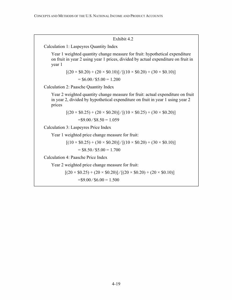
CONCEPTS AND METHODS OF THE U.S. NATIONAL INCOME AND PRODUCT ACCOUNTS
Exhibit 4.2
Calculation 1: Laspeyres Quantity Index
Year 1 weighted quantity change measure for fruit: hypothetical expenditure on fruit in year 2 using year 1 prices, divided by actual expenditure on fruit in year 1
[(20 × $0.20) + (20 × $0.10)] ⁄ [(10 × $0.20) + (30 × $0.10)]
= $6.00 ⁄ $5.00 = 1.200
Calculation 2: Paasche Quantity Index
Year 2 weighted quantity change measure for fruit: actual expenditure on fruit in year 2, divided by hypothetical expenditure on fruit in year 1 using year 2 prices
[(20 × $0.25) + (20 × $0.20)] ⁄ [(10 × $0.25) + (30 × $0.20)]
=$9.00 ⁄ $8.50 = 1.059
Calculation 3: Laspeyres Price Index
Year 1 weighted price change measure for fruit:
[(10 × $0.25) + (30 × $0.20)] ⁄ [(10 × $0.20) + (30 × $0.10)]
= $8.50 ⁄ $5.00 = 1.700
Calculation 4: Paasche Price Index
Year 2 weighted price change measure for fruit:
[(20 × $0.25) + (20 × $0.20)] ⁄ [(20 × $0.20) + (20 × $0.10)]
=$9.00 ⁄ $6.00 = 1.500
4-19
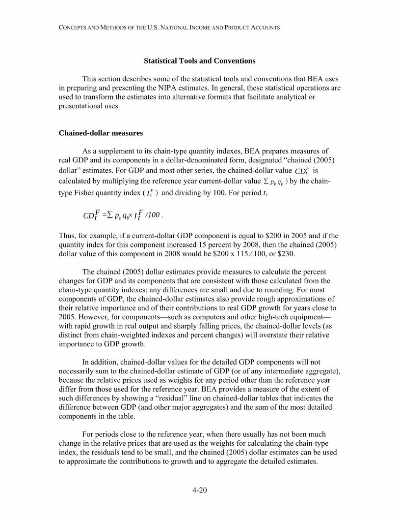
CONCEPTS AND METHODS OF THE U.S. NATIONAL INCOME AND PRODUCT ACCOUNTS
Statistical Tools and Conventions
This section describes some of the statistical tools and conventions that BEA uses in preparing and presenting the NIPA estimates. In general, these statistical operations are used to transform the estimates into alternative formats that facilitate analytical or presentational uses. Chained-dollar measures
As a supplement to its chain-type quantity indexes, BEA prepares measures of real GDP and its components in a dollar-denominated form, designated “chained (2005) dollar” estimates. For GDP and most other series, the chained-dollar value CD is calculated by multiplying the reference year current-dollar value
Ft
qp bb∑ )by the chain-type Fisher quantity index ( ) and dividing by 100. For period t, I F
t
/100I F
tqp=CD Ft bb ×∑ .
Thus, for example, if a current-dollar GDP component is equal to $200 in 2005 and if the quantity index for this component increased 15 percent by 2008, then the chained (2005) dollar value of this component in 2008 would be $200 x 115 ⁄ 100, or $230.
The chained (2005) dollar estimates provide measures to calculate the percent changes for GDP and its components that are consistent with those calculated from the chain-type quantity indexes; any differences are small and due to rounding. For most components of GDP, the chained-dollar estimates also provide rough approximations of their relative importance and of their contributions to real GDP growth for years close to 2005. However, for components—such as computers and other high-tech equipment—with rapid growth in real output and sharply falling prices, the chained-dollar levels (as distinct from chain-weighted indexes and percent changes) will overstate their relative importance to GDP growth.
In addition, chained-dollar values for the detailed GDP components will not
necessarily sum to the chained-dollar estimate of GDP (or of any intermediate aggregate), because the relative prices used as weights for any period other than the reference year differ from those used for the reference year. BEA provides a measure of the extent of such differences by showing a “residual” line on chained-dollar tables that indicates the difference between GDP (and other major aggregates) and the sum of the most detailed components in the table.
For periods close to the reference year, when there usually has not been much
change in the relative prices that are used as the weights for calculating the chain-type index, the residuals tend to be small, and the chained (2005) dollar estimates can be used to approximate the contributions to growth and to aggregate the detailed estimates.
4-20
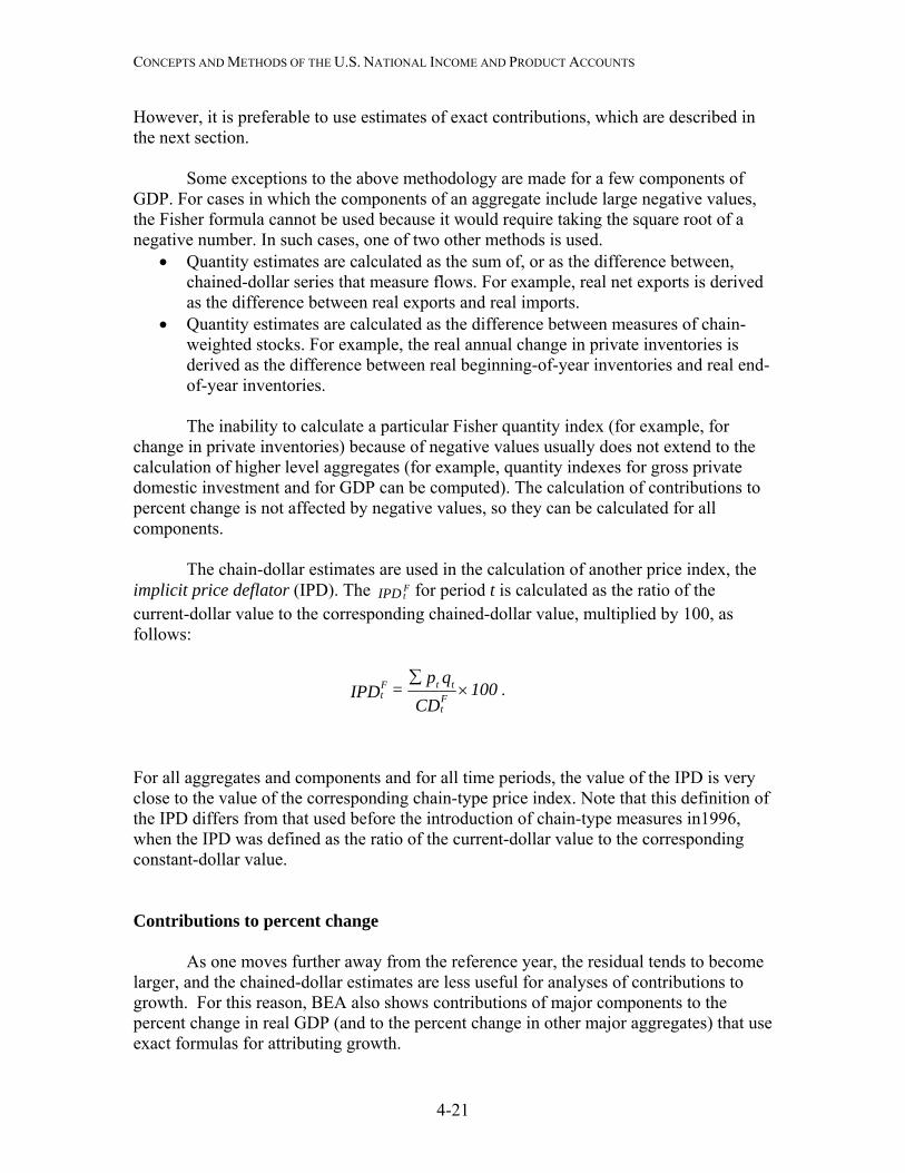
CONCEPTS AND METHODS OF THE U.S. NATIONAL INCOME AND PRODUCT ACCOUNTS
However, it is preferable to use estimates of exact contributions, which are described in the next section.
Some exceptions to the above methodology are made for a few components of
GDP. For cases in which the components of an aggregate include large negative values, the Fisher formula cannot be used because it would require taking the square root of a negative number. In such cases, one of two other methods is used.
• Quantity estimates are calculated as the sum of, or as the difference between, chained-dollar series that measure flows. For example, real net exports is derived as the difference between real exports and real imports.
• Quantity estimates are calculated as the difference between measures of chain-weighted stocks. For example, the real annual change in private inventories is derived as the difference between real beginning-of-year inventories and real end-of-year inventories.
The inability to calculate a particular Fisher quantity index (for example, for
change in private inventories) because of negative values usually does not extend to the calculation of higher level aggregates (for example, quantity indexes for gross private domestic investment and for GDP can be computed). The calculation of contributions to percent change is not affected by negative values, so they can be calculated for all components.
The chain-dollar estimates are used in the calculation of another price index, the
implicit price deflator (IPD). The for period t is calculated as the ratio of the current-dollar value to the corresponding chained-dollar value, multiplied by 100, as follows:
IPD Ft
100CD
qp=IPD F
t
ttFt ×
∑.
For all aggregates and components and for all time periods, the value of the IPD is very close to the value of the corresponding chain-type price index. Note that this definition of the IPD differs from that used before the introduction of chain-type measures in1996, when the IPD was defined as the ratio of the current-dollar value to the corresponding constant-dollar value.
Contributions to percent change
As one moves further away from the reference year, the residual tends to become
larger, and the chained-dollar estimates are less useful for analyses of contributions to growth. For this reason, BEA also shows contributions of major components to the percent change in real GDP (and to the percent change in other major aggregates) that use exact formulas for attributing growth.
4-21
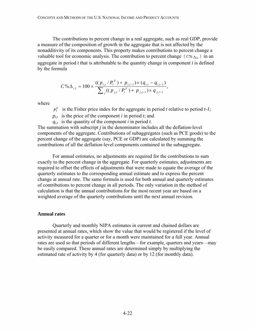
CONCEPTS AND METHODS OF THE U.S. NATIONAL INCOME AND PRODUCT ACCOUNTS
The contributions to percent change in a real aggregate, such as real GDP, provide
a measure of the composition of growth in the aggregate that is not affected by the nonadditivity of its components. This property makes contributions to percent change a valuable tool for economic analysis. The contribution to percent change ( ) in an aggregate in period t that is attributable to the quantity change in component i is defined by the formula
Δ ti,C%
,))/((
)())/((100%
1,1,,
1,,1,,, ∑ −−
−−
×+−×+
×=Δj tjtj
Fttj
tititiF
ttiti qpPp
qqpPpC
where
PFt is the Fisher price index for the aggregate in period t relative to period t-1;
pi,t is the price of the component i in period t; and qi,t is the quantity of the component i in period t.
The summation with subscript j in the denominator includes all the deflation-level components of the aggregate. Contributions of subaggregates (such as PCE goods) to the percent change of the aggregate (say, PCE or GDP) are calculated by summing the contributions of all the deflation-level components contained in the subaggregate.
For annual estimates, no adjustments are required for the contributions to sum exactly to the percent change in the aggregate. For quarterly estimates, adjustments are required to offset the effects of adjustments that were made to equate the average of the quarterly estimates to the corresponding annual estimate and to express the percent change at annual rate. The same formula is used for both annual and quarterly estimates of contributions to percent change in all periods. The only variation in the method of calculation is that the annual contributions for the most recent year are based on a weighted average of the quarterly contributions until the next annual revision. Annual rates Quarterly and monthly NIPA estimates in current and chained dollars are presented at annual rates, which show the value that would be registered if the level of activity measured for a quarter or for a month were maintained for a full year. Annual rates are used so that periods of different lengths—for example, quarters and years—may be easily compared. These annual rates are determined simply by multiplying the estimated rate of activity by 4 (for quarterly data) or by 12 (for monthly data).
4-22
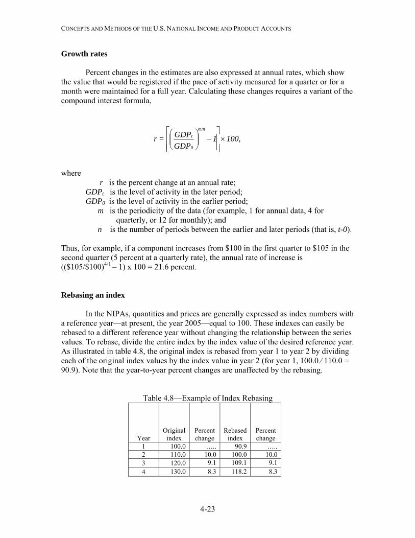
CONCEPTS AND METHODS OF THE U.S. NATIONAL INCOME AND PRODUCT ACCOUNTS
4-23
Growth rates
Percent changes in the estimates are also expressed at annual rates, which show the value that would be registered if the pace of activity measured for a quarter or for a month were maintained for a full year. Calculating these changes requires a variant of the compound interest formula,
100,1GDPGDP=r
0
tm/n
×⎥⎥⎦
⎤
⎢⎢⎣
⎡⎟⎟⎠
⎞⎜⎜⎝
⎛ –
where
r is the percent change at an annual rate; GDPt is the level of activity in the later period; GDP0 is the level of activity in the earlier period; m is the periodicity of the data (for example, 1 for annual data, 4 for quarterly, or 12 for monthly); and n is the number of periods between the earlier and later periods (that is, t-0). Thus, for example, if a component increases from $100 in the first quarter to $105 in the second quarter (5 percent at a quarterly rate), the annual rate of increase is (($105/$100)4/1 – 1) x 100 = 21.6 percent. Rebasing an index In the NIPAs, quantities and prices are generally expressed as index numbers with a reference year—at present, the year 2005—equal to 100. These indexes can easily be rebased to a different reference year without changing the relationship between the series values. To rebase, divide the entire index by the index value of the desired reference year. As illustrated in table 4.8, the original index is rebased from year 1 to year 2 by dividing each of the original index values by the index value in year 2 (for year 1, 100.0 ⁄ 110.0 = 90.9). Note that the year-to-year percent changes are unaffected by the rebasing.
Table 4.8—Example of Index Rebasing
Year Original
index
Percent change
Rebased index
Percent change
1 100.0 ….. 90.9 ….. 2 110.0 10.0 100.0 10.0 3 120.0 9.1 109.1 9.1 4 130.0 8.3 118.2 8.3
CHAPTER 5: PERSONAL CONSUMPTION EXPENDITURES Definitions and Concepts Recording in the NIPAs Overview of Source Data and Estimating Methods Benchmark-year estimates
Nonbenchmark-year estimates Current quarterly and monthly estimates Quantity and price estimates
Table 5.A—Summary of Methodology for PCE for Goods Table 5.B—Summary of Methodology for PCE for Services
Technical Note: Special Estimates New motor vehicles Net purchases of used motor vehicles Motor vehicle fuels Rental of tenant- and owner-occupied nonfarm housing Financial service charges and fees Securities commissions Financial services furnished without payment
Life insurance Property and casualty insurance Nonprofit institutions serving households
Personal consumption expenditures (PCE) is the primary measure of consumer spending on goods and services in the U.S. economy.1 It accounts for about two-thirds of domestic final spending, and thus it is the primary engine that drives future economic growth. PCE shows how much of the income earned by households is being spent on current consumption as opposed to how much is being saved for future consumption. PCE also provides a comprehensive measure of types of goods and services that are purchased by households. Thus, for example, it shows the portion of spending that is accounted for by discretionary items, such as motor vehicles, or the adjustments that consumers make to changes in prices, such as a sharp run-up in gasoline prices. In addition, the PCE estimates are available monthly, so they can provide an early indication of the course of economic activity in the current quarter. For example the PCE estimates for January are released at the end of February, and the estimates for February are released at the end of March; the advance estimates of gross domestic product (GDP) for the first quarter are released at the end of April. 1 For a comprehensive presentation of BEA’s information on PCE, go to www.bea.gov, look under “National” accounts, and click on “Consumer Spending.”
5-1
The PCE estimates are an integral part of the U.S. national income and product accounts (NIPAs), a set of accounts that provide a logical and consistent framework for presenting statistics on U.S. economic activity (see “Chapter 2: Fundamental Concepts”).
Definitions and Concepts PCE measures the goods and services purchased by “persons”—that is, by
households and by nonprofit institutions serving households (NPISHs)—who are resident in the United States. Persons resident in the United States are those who are physically located in the United States and who have resided, or expect to reside, in this country for 1 year or more. PCE also includes purchases by U.S. government civilian and military personnel stationed abroad, regardless of the duration of their assignments, and by U.S. residents who are traveling or working abroad for 1 year or less.
Table 5.1 shows the kinds of transactions that are included in and excluded from PCE. Most of PCE consists of purchases of new goods and of services by households from private business. In addition, PCE includes purchases of new goods and of services by households from government and government enterprises, the costs incurred by NPISHs in providing services on behalf of households, net purchases of used goods by households, and purchases abroad of goods and services by U.S. residents traveling, working, or attending school in foreign countries. PCE also includes expenditures financed by third-party payers on behalf of households, such as employer-paid health insurance and medical care financed through government programs, and it includes expenses associated with life insurance and with private and government employee pension plans. Finally, PCE includes imputed purchases that keep PCE invariant to changes in the way that certain activities are carried out—for example, whether housing is rented or owned or whether employees are paid in cash or in kind.2 PCE transactions are valued in market prices, including sales and excise taxes. In the NIPAs, final consumption expenditures by NPISHs is the portion of PCE that represents the services that are provided to households by NPISHs without explicit charge (such as the value of the education services provided by a nonprofit college or university that is over and above the tuition and other costs paid by or for the student’s household). It is equal to their gross output, which is measured as their current operating expenses (not including purchases of buildings and equipment, which are treated as private fixed investment), less their sales to households and to other sectors of the economy (such as sales of education services to employers) and less the value of any investment goods (such as software) that are produced directly by the NPISH. Services that are provided by NPISHs and are paid by or on behalf of households (such as the tuition and other costs) are already accounted for in PCE as purchases by households. (For more information, see the section on NPISHs in the technical note at the end of this chapter.) 2 See Larry R. Moran and Clinton P. McCully, “Trends in Consumer Spending: 1959–2000,” Survey of Current Business 81 (March 2001): 15–21.
5-2
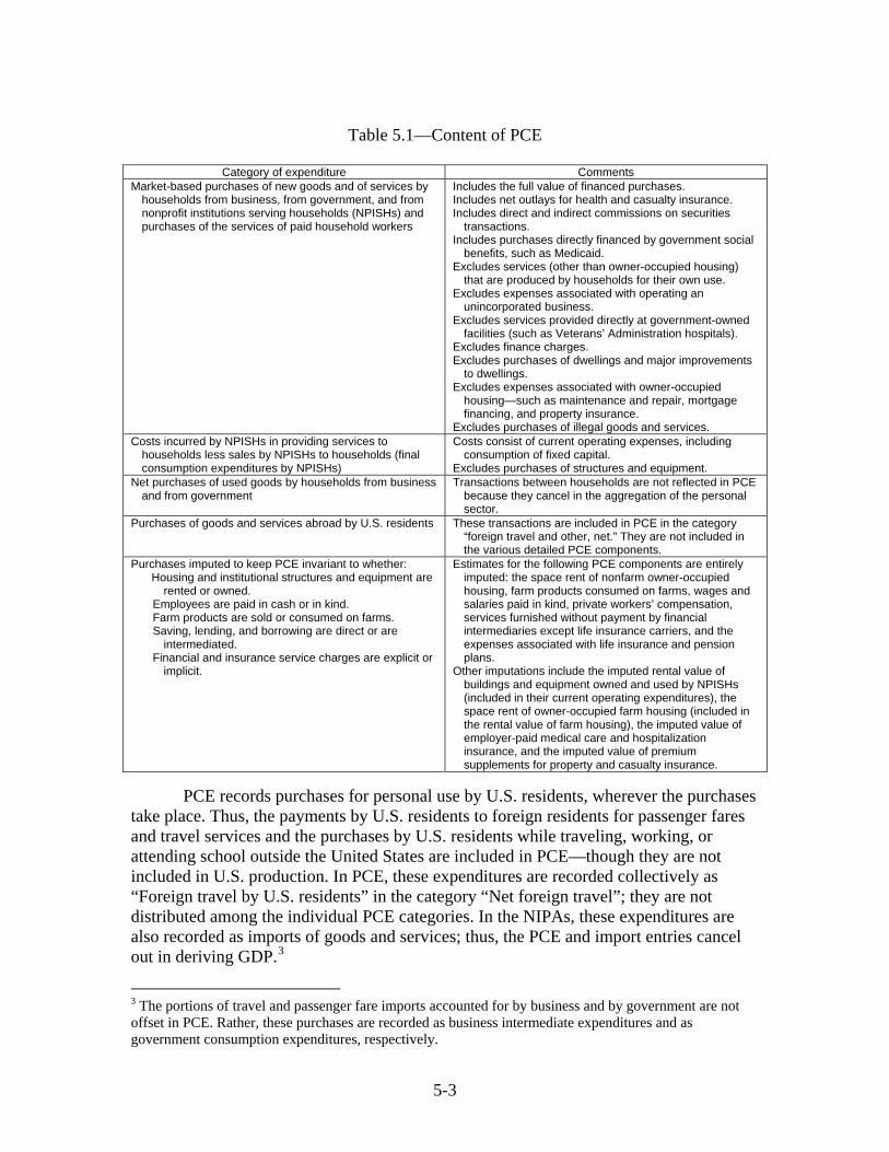
Table 5.1—Content of PCE
Category of expenditure Comments
Market-based purchases of new goods and of services by households from business, from government, and from nonprofit institutions serving households (NPISHs) and purchases of the services of paid household workers
Includes the full value of financed purchases. Includes net outlays for health and casualty insurance. Includes direct and indirect commissions on securities
transactions. Includes purchases directly financed by government social
benefits, such as Medicaid. Excludes services (other than owner-occupied housing)
that are produced by households for their own use. Excludes expenses associated with operating an
unincorporated business. Excludes services provided directly at government-owned
facilities (such as Veterans’ Administration hospitals). Excludes finance charges. Excludes purchases of dwellings and major improvements
to dwellings. Excludes expenses associated with owner-occupied
housing—such as maintenance and repair, mortgage financing, and property insurance.
Excludes purchases of illegal goods and services. Costs incurred by NPISHs in providing services to
households less sales by NPISHs to households (final consumption expenditures by NPISHs)
Costs consist of current operating expenses, including consumption of fixed capital.
Excludes purchases of structures and equipment. Net purchases of used goods by households from business
and from government Transactions between households are not reflected in PCE
because they cancel in the aggregation of the personal sector.
Purchases of goods and services abroad by U.S. residents These transactions are included in PCE in the category “foreign travel and other, net.” They are not included in the various detailed PCE components.
Purchases imputed to keep PCE invariant to whether: Housing and institutional structures and equipment are
rented or owned. Employees are paid in cash or in kind. Farm products are sold or consumed on farms. Saving, lending, and borrowing are direct or are
intermediated. Financial and insurance service charges are explicit or
implicit.
Estimates for the following PCE components are entirely imputed: the space rent of nonfarm owner-occupied housing, farm products consumed on farms, wages and salaries paid in kind, private workers’ compensation, services furnished without payment by financial intermediaries except life insurance carriers, and the expenses associated with life insurance and pension plans.
Other imputations include the imputed rental value of buildings and equipment owned and used by NPISHs (included in their current operating expenditures), the space rent of owner-occupied farm housing (included in the rental value of farm housing), the imputed value of employer-paid medical care and hospitalization insurance, and the imputed value of premium supplements for property and casualty insurance.
PCE records purchases for personal use by U.S. residents, wherever the purchases take place. Thus, the payments by U.S. residents to foreign residents for passenger fares and travel services and the purchases by U.S. residents while traveling, working, or attending school outside the United States are included in PCE—though they are not included in U.S. production. In PCE, these expenditures are recorded collectively as “Foreign travel by U.S. residents” in the category “Net foreign travel”; they are not distributed among the individual PCE categories. In the NIPAs, these expenditures are also recorded as imports of goods and services; thus, the PCE and import entries cancel out in deriving GDP.3
3 The portions of travel and passenger fare imports accounted for by business and by government are not offset in PCE. Rather, these purchases are recorded as business intermediate expenditures and as government consumption expenditures, respectively.
5-3
Conversely, the payments by foreign residents to U.S. residents for travel services and the purchases by foreign residents while traveling, working, attending school, or receiving medical treatment in the United States are not included in PCE—though they are included in U.S. production. However, these expenditures are included in the source data that underlie the estimates of most individual PCE categories, where they are indistinguishable from expenditures made by U.S. residents.4 In order to exclude these expenditures from PCE, they are recorded collectively as “Less: Expenditures in the United States by nonresidents” in the category “Net foreign travel”; this entry negates the expenditures by foreign residents that are embedded in the source data. In the NIPAs, the expenditures by foreign residents are also recorded as exports of goods and services; thus, they are included in deriving GDP.
PCE is classified by type of product as follows. Goods are tangible commodities that can be stored or inventoried. Durable goods are goods that have an average useful life of at least 3 years. Nondurable goods are goods that have an average useful life of less than 3 years. Services are commodities that cannot be stored or inventoried and that are usually consumed at the place and time of purchase.
In the 2009 comprehensive revision of the NIPAs, BEA introduced a new classification system for PCE.5 This system reflects long-term changes in consumption patterns due to shifts in consumer demographics, income, and tastes; to the increased importance of services; and to the introduction of a wide variety of new products. The system follows recommendations for the classification of household and nonprofit consumption by the international System of National Accounts (SNA), thus improving consistency with international standards.
In the new system, PCE by type of product is classified into the following broad
categories. • Durable goods: motor vehicles and parts, furnishings and durable household
equipment, recreational goods and vehicles, and other durable goods. • Nondurable goods: food and beverages purchased for off-premises consumption,
clothing and footwear, gasoline and other energy goods, and other nondurable goods.
• Services: housing and utilities, health care, transportation services, recreation services, food services and accommodations, financial services and insurance, and other services.
PCE by function is classified into the following broad categories:
4 Passenger fares paid by foreign residents to U.S. carriers for transportation to and from the United States are not included in any of the PCE categories; these expenditures are recorded as exports in the NIPAs. Foreign residents’ expenditures for transportation within the United States are recorded in both exports and PCE for public transportation. 5 See Clinton P. McCully and Teresita D. Teensma, “Preview of the 2009 Comprehensive Revision of the National Income and Product Accounts: New Classifications for Personal Consumption Expenditures,” Survey 88 (May 2008): 6–17.
5-4

• Food and beverages purchased for off-premises consumption • Clothing, footwear, and related services • Housing, utilities, and fuels • Furnishings, household equipment, and routine household maintenance • Health • Transportation • Communication • Recreation • Education • Food service and accommodations • Financial services and insurance • Other goods and services • Net foreign travel and expenditures abroad by U.S. residents
In addition, household consumption expenditures and the final consumption expenditures of NPISHs are now shown separately in the PCE tables. Household consumption expenditures comprise purchases from business, government, and the rest of the world and from NPISHs (which are included in the health, recreation, education, and “other goods and services” categories). Final consumption expenditures of NPISHs are measured as gross output less own-account investment and less sales to households and other sectors (see the technical note).
Recording in the NIPAs As described in chapter 2, the NIPAs can be viewed as aggregations of accounts belonging to individual transactors in the economy. Thus, PCE represents the final demand for goods and services by households and NPISHs. In the seven summary accounts of the NIPAs, PCE appears in the Domestic Income and Product Account (Account 1), where it is the largest component of final demand, and in the Personal Income and Outlay Account (Account 3), where it is the dominant outlay. In the NIPAs, PCE by major type of product is presented in NIPA table group 2.3, and more detailed information by type of product is presented in NIPA table group 2.4. This presentation is based on the classification of the PCE categories into durable goods, nondurable goods, and services (for more information, see the section “Type of product” in chapter 2). PCE by function is presented in NIPA table group 2.5. This presentation is based on the classification of the PCE categories into broad expenditure categories (for more information, see “Function” in chapter 2). PCE by type of product on a monthly basis is presented in NIPA table group 2.8. In addition, separate annual estimates for the income and outlays of households and of NPISHs are provided in NIPA table group 2.9. The following is a list of the principal NIPA tables that present the PCE estimates: 2.3.1 Percent Change From Preceding Period in Real Personal Consumption
Expenditures by Major Type of Product
5-5
2.3.2 Contributions to Percent Change in Real Personal Consumption Expenditures by Major Type of Product
2.3.3 Real Personal Consumption Expenditures by Major Type of Product, Quantity Indexes
2.3.4 Price Indexes for Personal Consumption Expenditures by Major Type of Product 2.3.5 Personal Consumption Expenditures by Major Type of Product 2.3.6 Real Personal Consumption Expenditures by Major Type of Product, Chained
Dollars 2.3.7 Percent Change from Preceding Period in Prices for Personal Consumption
Expenditures by Major Type of Product 2.4.3 Real Personal Consumption Expenditures by Type of Product, Quantity Indexes 2.4.4 Price Indexes for Personal Consumption Expenditures by Type of Product 2.4.5 Personal Consumption Expenditures by Type of Product 2.4.6 Real Personal Consumption Expenditures by Type of Product, Chained Dollars 2.5.3 Real Personal Consumption Expenditures by Function, Quantity Indexes 2.5.4 Price Indexes for Personal Consumption Expenditures by Function 2.5.5 Personal Consumption Expenditures by Function 2.5.6 Real Personal Consumption Expenditures by Function, Chained Dollars 2.8.1 Percent Change From Preceding Period in Real Personal Consumption
Expenditures by Major Type of Product, Monthly 2.8.3 Real Personal Consumption Expenditures by Major Type of Product, Monthly,
Quantity Indexes 2.8.4 Price Indexes for Personal Consumption Expenditures by Major Type of Product,
Monthly 2.8.5 Personal Consumption Expenditures by Major Type of Product, Monthly 2.8.6 Real Personal Consumption Expenditures by Major Type of Product, Monthly,
Chained Dollars 2.8.7 Percent Change from Preceding Period in Prices for Personal Consumption
Expenditures by Major Type of Product, Monthly 2.9 Personal Income and Its Disposition by Households and by Nonprofit Institutions
Serving Households BEA also prepares “Underlying Detail Tables” for PCE by type of product that provide current-dollar, chained-dollar, and price estimates at a greater level of detail than are shown in the above tables. BEA does not include these detailed estimates in the published tables because their quality is significantly lower than that of the higher level categories of which they are a part. In particular, these detailed estimates are more likely to be based on judgmental trends or on less reliable source data.
Overview of Source Data and Estimating Methods As described earlier, the NIPA estimates, including those for PCE, are prepared using a wide variety of source data (see “Chapter 3: Principal Source Data”) and using estimating methods that adjust the source data to the required NIPA concepts and that fill in gaps in coverage and timing (see “Chapter 4: Estimating Methods”). For PCE, the
5-6
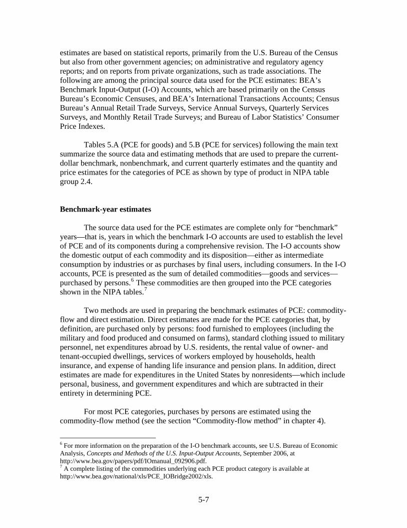
estimates are based on statistical reports, primarily from the U.S. Bureau of the Census but also from other government agencies; on administrative and regulatory agency reports; and on reports from private organizations, such as trade associations. The following are among the principal source data used for the PCE estimates: BEA’s Benchmark Input-Output (I-O) Accounts, which are based primarily on the Census Bureau’s Economic Censuses, and BEA’s International Transactions Accounts; Census Bureau’s Annual Retail Trade Surveys, Service Annual Surveys, Quarterly Services Surveys, and Monthly Retail Trade Surveys; and Bureau of Labor Statistics’ Consumer Price Indexes. Tables 5.A (PCE for goods) and 5.B (PCE for services) following the main text summarize the source data and estimating methods that are used to prepare the current-dollar benchmark, nonbenchmark, and current quarterly estimates and the quantity and price estimates for the categories of PCE as shown by type of product in NIPA table group 2.4. Benchmark-year estimates The source data used for the PCE estimates are complete only for “benchmark” years—that is, years in which the benchmark I-O accounts are used to establish the level of PCE and of its components during a comprehensive revision. The I-O accounts show the domestic output of each commodity and its disposition—either as intermediate consumption by industries or as purchases by final users, including consumers. In the I-O accounts, PCE is presented as the sum of detailed commodities—goods and services—purchased by persons.6 These commodities are then grouped into the PCE categories shown in the NIPA tables.7
Two methods are used in preparing the benchmark estimates of PCE: commodity-flow and direct estimation. Direct estimates are made for the PCE categories that, by definition, are purchased only by persons: food furnished to employees (including the military and food produced and consumed on farms), standard clothing issued to military personnel, net expenditures abroad by U.S. residents, the rental value of owner- and tenant-occupied dwellings, services of workers employed by households, health insurance, and expense of handing life insurance and pension plans. In addition, direct estimates are made for expenditures in the United States by nonresidents—which include personal, business, and government expenditures and which are subtracted in their entirety in determining PCE.
For most PCE categories, purchases by persons are estimated using the commodity-flow method (see the section “Commodity-flow method” in chapter 4).
6 For more information on the preparation of the I-O benchmark accounts, see U.S. Bureau of Economic Analysis, Concepts and Methods of the U.S. Input-Output Accounts, September 2006, at http://www.bea.gov/papers/pdf/IOmanual_092906.pdf. 7 A complete listing of the commodities underlying each PCE product category is available at http://www.bea.gov/national/xls/PCE_IOBridge2002/xls.
5-7
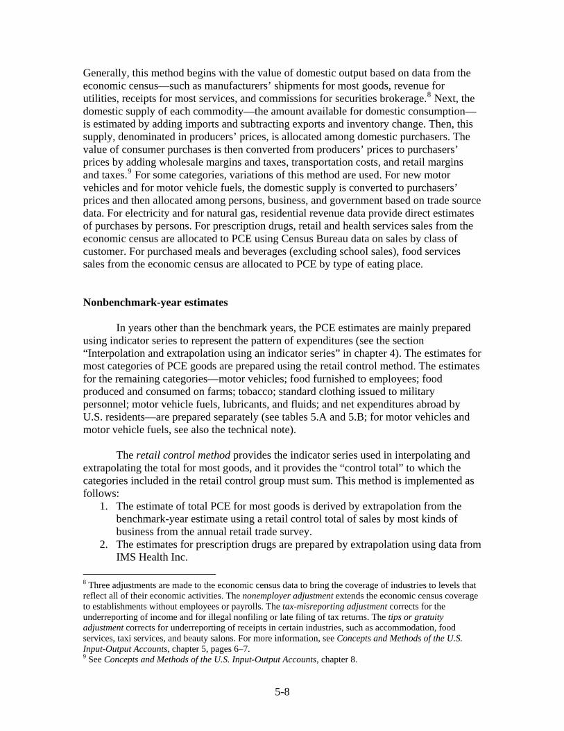
Generally, this method begins with the value of domestic output based on data from the economic census—such as manufacturers’ shipments for most goods, revenue for utilities, receipts for most services, and commissions for securities brokerage.8 Next, the domestic supply of each commodity—the amount available for domestic consumption—is estimated by adding imports and subtracting exports and inventory change. Then, this supply, denominated in producers’ prices, is allocated among domestic purchasers. The value of consumer purchases is then converted from producers’ prices to purchasers’ prices by adding wholesale margins and taxes, transportation costs, and retail margins and taxes.9 For some categories, variations of this method are used. For new motor vehicles and for motor vehicle fuels, the domestic supply is converted to purchasers’ prices and then allocated among persons, business, and government based on trade source data. For electricity and for natural gas, residential revenue data provide direct estimates of purchases by persons. For prescription drugs, retail and health services sales from the economic census are allocated to PCE using Census Bureau data on sales by class of customer. For purchased meals and beverages (excluding school sales), food services sales from the economic census are allocated to PCE by type of eating place. Nonbenchmark-year estimates
In years other than the benchmark years, the PCE estimates are mainly prepared using indicator series to represent the pattern of expenditures (see the section “Interpolation and extrapolation using an indicator series” in chapter 4). The estimates for most categories of PCE goods are prepared using the retail control method. The estimates for the remaining categories—motor vehicles; food furnished to employees; food produced and consumed on farms; tobacco; standard clothing issued to military personnel; motor vehicle fuels, lubricants, and fluids; and net expenditures abroad by U.S. residents—are prepared separately (see tables 5.A and 5.B; for motor vehicles and motor vehicle fuels, see also the technical note).
The retail control method provides the indicator series used in interpolating and
extrapolating the total for most goods, and it provides the “control total” to which the categories included in the retail control group must sum. This method is implemented as follows:
1. The estimate of total PCE for most goods is derived by extrapolation from the benchmark-year estimate using a retail control total of sales by most kinds of business from the annual retail trade survey.
2. The estimates for prescription drugs are prepared by extrapolation using data from IMS Health Inc.
8 Three adjustments are made to the economic census data to bring the coverage of industries to levels that reflect all of their economic activities. The nonemployer adjustment extends the economic census coverage to establishments without employees or payrolls. The tax-misreporting adjustment corrects for the underreporting of income and for illegal nonfiling or late filing of tax returns. The tips or gratuity adjustment corrects for underreporting of receipts in certain industries, such as accommodation, food services, taxi services, and beauty salons. For more information, see Concepts and Methods of the U.S. Input-Output Accounts, chapter 5, pages 6–7. 9 See Concepts and Methods of the U.S. Input-Output Accounts, chapter 8.
5-8

3. The estimates for the rest of the detailed PCE categories are prepared by extrapolation using estimates of retail sales by corresponding product lines that, in turn, are based on commodity sales data from the most recent economic census. For goods bought at grocery stores, the economic census allocations are updated annually using retail point-of-sale scanner data from Information Resources, Inc.10 For goods bought at radio, television, and electronics stores, at computer and software stores, and at camera and photographic supply stores, the allocations are updated using retail point-of-sale scanner data from NPD Group.11
4. The expenditures estimates for the categories in step 3 are adjusted proportionately so that their sum plus the expenditures for prescription drugs is equal to the retail control total in step 1.
(For a general illustration of this method, see the section “Retail control method” in chapter 4.)
A variety of sources and methods are used to construct the indicator series for the PCE services categories. For many services, the service annual survey is the primary data source. Current quarterly and monthly estimates The current dollar quarterly and monthly estimates for most PCE categories are prepared by using indicator series to extrapolate from the annual estimates. Most goods categories are estimated by the retail control method using data on retail sales from the monthly retail trade survey (MRTS).12 The rest of the goods categories are estimated using other indicator series.
For services categories for which source data are not available to prepare an indicator series, the current estimates are extrapolated based on trends and on judgment by BEA analysts. In general, the real-dollar series for these categories are extrapolated using the rate of change in population and a projected rate of change in real per capita consumption based on the results of the most recent NIPA annual revision. The real-dollar estimates are then converted to current dollars using the appropriate monthly price indexes. Quantity and price estimates The estimates of quantities purchased, or real spending, for most of the detailed PCE categories are prepared by deflation. In this method, the quantities are calculated by
10 See Eugene P. Seskin and Shelly Smith, “Annual Revision of the National Income and Product Accounts,” Survey 88 (August 2008): 18. 11 See Clinton P. McCully and Steven Payson, “Preview of the 2009 Comprehensive Revision of the NIPAs: Statistical Changes,” Survey 89 (May 2009): 9. 12 For the advance quarterly estimate, the source data for the third month are from the Census Bureau’s advance monthly retail sales survey because the MRTS data are not yet available.
5-9
5-10
dividing the current-dollar value of the component by an appropriate price index (with the reference-year value set to 100). For most PCE categories, the closest matching price index is a consumer price index or indexes. In addition, the quantity estimates for some detailed components are prepared by quantity extrapolation or by direct valuation. (For descriptions of the three methods, see the section “Estimates for detailed components” in chapter 4.) The aggregate PCE measures are calculated from the detailed components as chain-type quantity and price indexes (for information about these calculations, see the section “Estimates for NIPA aggregates” in chapter 4). BEA also prepares measures of real PCE and its components in a dollar-denominated form, designated “chained-dollar” estimates (see “Chained-dollar measures” in chapter 4).
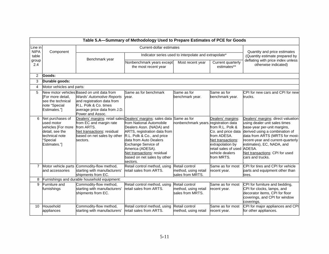
Table 5.A—Summary of Methodology Used to Prepare Estimates of PCE for Goods Current-dollar estimates
Indicator series used to interpolate and extrapolate*
Line in NIPA table group
2.4
Component
Benchmark year
Nonbenchmark years except the most recent year
Most recent year
Current quarterly estimates**
Quantity and price estimates
(Quantity estimate prepared by deflating with price index unless
otherwise indicated)
2 Goods: 3 Durable goods: 4 Motor vehicles and parts: 5 New motor vehicles
[For more detail, see the technical note “Special Estimates.”]
Based on unit data from Wards’ Automotive Reports and registration data from R.L. Polk & Co. times average price data from J.D. Power and Assoc.
Same as for benchmark year.
Same as for benchmark year.
Same as for benchmark year.
CPI for new cars and CPI for new trucks.
6 Net purchases of used motor vehicles [For more detail, see the technical note “Special Estimates.”]
Dealers’ margins: retail sales from EC and margin rate from ARTS. Net transactions: residual based on net sales by other sectors.
Dealers' margins: sales data from National Automobile Dealers Assn. (NADA) and ARTS, registration data from R.L. Polk & Co., and price data from Auto Dealers Exchange Service of America (ADESA). Net transactions: residual based on net sales by other sectors.
Same as for nonbenchmark years.
Dealers’ margins: registration data from R.L. Polk & Co. and price data from ADESA. Net transactions: extrapolation by retail sales of used vehicle dealers from MRTS.
Dealers’ margins: direct valuationusing dealer unit sales times base-year per-unit margins, derived using a combination of data from ARTS (MRTS for most-recent-year and current-quarterly estimates), EC, NADA, and ADESA. Net transactions: CPI for used cars and trucks. .
7 Motor vehicle parts and accessories
Commodity-flow method, starting with manufacturers’ shipments from EC.
Retail control method, using retail sales from ARTS.
Retail control method, using retail sales from MRTS.
Same as for most recent year.
CPI for tires and CPI for vehicle parts and equipment other than tires.
8 Furnishings and durable household equipment: 9 Furniture and
furnishings Commodity-flow method, starting with manufacturers’ shipments from EC.
Retail control method, using retail sales from ARTS.
Retail control method, using retail sales from MRTS.
Same as for most recent year.
CPI for furniture and bedding, CPI for clocks, lamps, and decorator items, CPI for floor coverings, and CPI for window coverings.
10 Household appliances
Commodity-flow method, starting with manufacturers’
Retail control method, using retail sales from ARTS.
Retail control method, using retail
Same as for most recent year.
CPI for major appliances and CPI for other appliances.
5-11
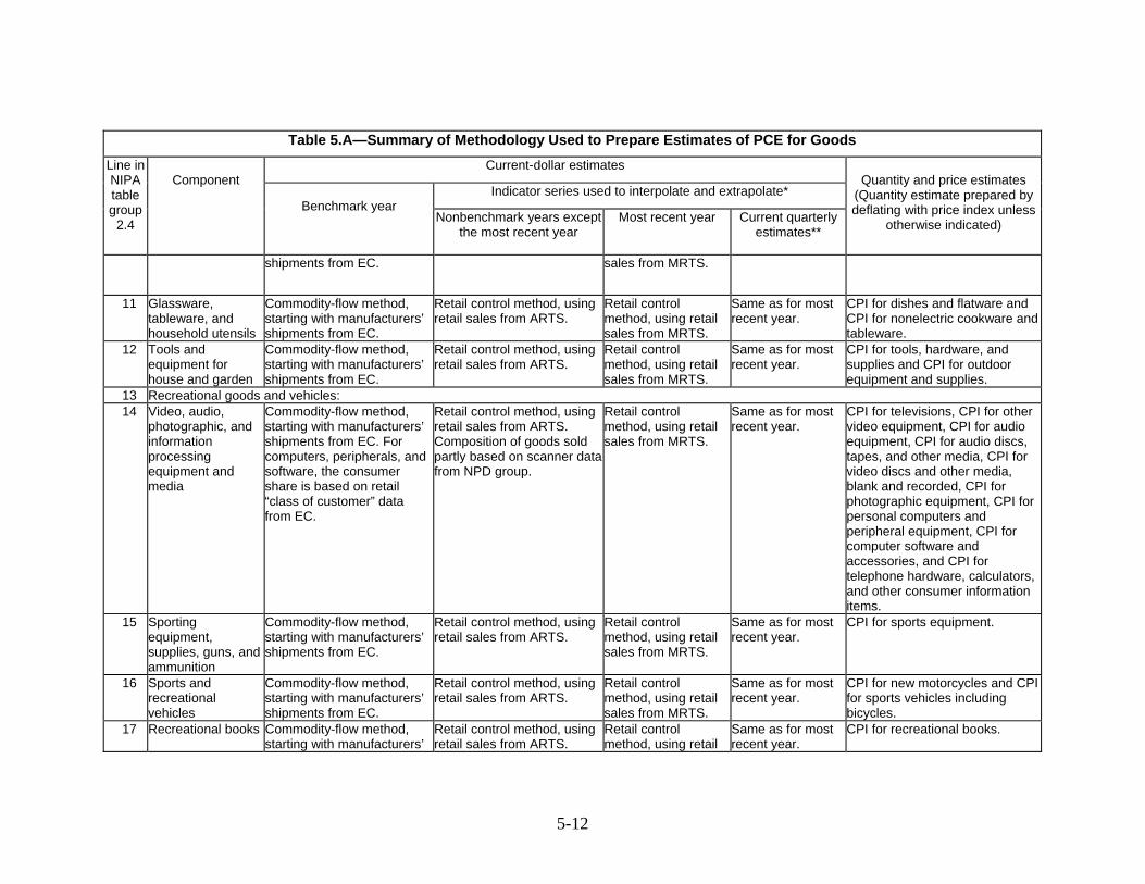
Table 5.A—Summary of Methodology Used to Prepare Estimates of PCE for Goods Current-dollar estimates
Indicator series used to interpolate and extrapolate*
Line in NIPA table group
2.4
Component
Benchmark year
Nonbenchmark years except the most recent year
Most recent year
Current quarterly estimates**
Quantity and price estimates
(Quantity estimate prepared by deflating with price index unless
otherwise indicated)
shipments from EC. sales from MRTS.
11 Glassware, tableware, and household utensils
Commodity-flow method, starting with manufacturers’ shipments from EC.
Retail control method, using retail sales from ARTS.
Retail control method, using retail sales from MRTS.
Same as for most recent year.
CPI for dishes and flatware and CPI for nonelectric cookware and tableware.
12 Tools and equipment for house and garden
Commodity-flow method, starting with manufacturers’ shipments from EC.
Retail control method, using retail sales from ARTS.
Retail control method, using retail sales from MRTS.
Same as for most recent year.
CPI for tools, hardware, and supplies and CPI for outdoor equipment and supplies.
13 Recreational goods and vehicles: 14 Video, audio,
photographic, and information processing equipment and media
Commodity-flow method, starting with manufacturers’ shipments from EC. For computers, peripherals, and software, the consumer share is based on retail “class of customer” data from EC.
Retail control method, using retail sales from ARTS. Composition of goods sold partly based on scanner datafrom NPD group.
Retail control method, using retail sales from MRTS.
Same as for most recent year.
CPI for televisions, CPI for other video equipment, CPI for audio equipment, CPI for audio discs, tapes, and other media, CPI for video discs and other media, blank and recorded, CPI for photographic equipment, CPI for personal computers and peripheral equipment, CPI for computer software and accessories, and CPI for telephone hardware, calculators, and other consumer information items.
15 Sporting equipment, supplies, guns, and ammunition
Commodity-flow method, starting with manufacturers’ shipments from EC.
Retail control method, using retail sales from ARTS.
Retail control method, using retail sales from MRTS.
Same as for most recent year.
CPI for sports equipment.
16 Sports and recreational vehicles
Commodity-flow method, starting with manufacturers’ shipments from EC.
Retail control method, using retail sales from ARTS.
Retail control method, using retail sales from MRTS.
Same as for most recent year.
CPI for new motorcycles and CPI for sports vehicles including bicycles.
17 Recreational books Commodity-flow method, starting with manufacturers’
Retail control method, using retail sales from ARTS.
Retail control method, using retail
Same as for most recent year.
CPI for recreational books.
5-12

Table 5.A—Summary of Methodology Used to Prepare Estimates of PCE for Goods Current-dollar estimates
Indicator series used to interpolate and extrapolate*
Line in NIPA table group
2.4
Component
Benchmark year
Nonbenchmark years except the most recent year
Most recent year
Current quarterly estimates**
Quantity and price estimates
(Quantity estimate prepared by deflating with price index unless
otherwise indicated)
shipments from EC. sales from MRTS. 18 Musical instruments Commodity-flow method,
starting with manufacturers’ shipments from EC.
Retail control method, using retail sales from ARTS.
Retail control method, using retail sales from MRTS.
Same as for most recent year.
CPI for music instruments and accessories.
19 Other durable goods: 20 Jewelry and
watches Commodity-flow method, starting with manufacturers’ shipments from EC.
Retail control method, using retail sales from ARTS.
Retail control method, using retail sales from MRTS.
Same as for most recent year.
CPI for jewelry and CPI for watches.
21 Therapeutic appliances and equipment
Commodity-flow method, starting with manufacturers’ shipments from EC.
Retail control method, using retail sales from ARTS.
Retail control method, using retail sales from MRTS.
Same as for most recent year.
CPI for medical equipment and supplies and CPI for eyeglasses and eye care.
22 Educational books Commodity-flow method, starting with manufacturers’ shipments from EC.
Retail control method, using retail sales from ARTS.
Retail control method, using retail sales from MRTS.
Same as for most recent year.
CPI for educational books and supplies.
23 Luggage and similar personal items
Commodity-flow method, starting with manufacturers’ shipments from EC.
Retail control method, using retail sales from ARTS.
Retail control method, using retail sales from MRTS.
Same as for most recent year.
CPI for miscellaneous personal goods.
24 Telephone and facsimile equipment
Commodity-flow method, starting with manufacturers’ shipments from EC.
Retail control method, using retail sales from ARTS.
Retail control method, using retail sales from MRTS.
Same as for most recent year.
CPI for telephone hardware, calculators, and other consumer information items.
25 Nondurable goods: 26 Food and beverages purchased for off-premises consumption: 27 Food and
nonalcoholic beverages purchased for off-premises consumption
Commodity-flow method, starting with manufacturers’ shipments from EC.
Retail control method, using retail sales from ARTS. Composition of goods sold largely based on scanner data from Information Resources, Inc. and from Fresh Look Marketing Group.
Retail control method, using retail sales from MRTS.
Same as for most recent year.
Detailed price components of the CPI for food at home.
28 Alcoholic beverages
Commodity-flow method, starting with manufacturers’
Retail control method, using retail sales from ARTS.
Retail control method, using retail
Same as for most recent year.
CPI for distilled spirits at home, CPI for wine at home, and CPI
5-13
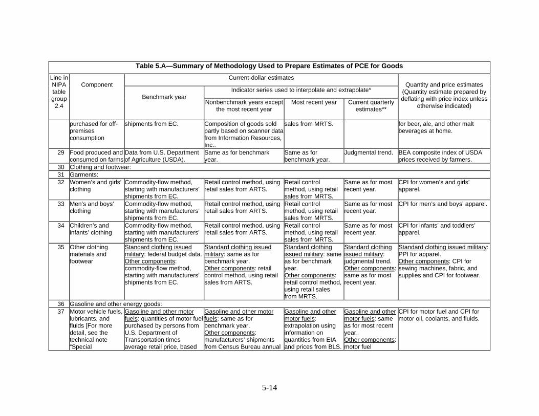
Table 5.A—Summary of Methodology Used to Prepare Estimates of PCE for Goods Current-dollar estimates
Indicator series used to interpolate and extrapolate*
Line in NIPA table group
2.4
Component
Benchmark year
Nonbenchmark years except the most recent year
Most recent year
Current quarterly estimates**
Quantity and price estimates
(Quantity estimate prepared by deflating with price index unless
otherwise indicated)
purchased for off-premises consumption
shipments from EC. Composition of goods sold partly based on scanner datafrom Information Resources, Inc..
sales from MRTS. for beer, ale, and other malt
beverages at home.
29 Food produced and consumed on farms
Data from U.S. Department of Agriculture (USDA).
Same as for benchmark year.
Same as for benchmark year.
Judgmental trend. BEA composite index of USDA prices received by farmers.
30 Clothing and footwear: 31 Garments: 32 Women’s and girls’
clothing Commodity-flow method, starting with manufacturers’ shipments from EC.
Retail control method, using retail sales from ARTS.
Retail control method, using retail sales from MRTS.
Same as for most recent year.
CPI for women’s and girls’ apparel.
33 Men’s and boys’ clothing
Commodity-flow method, starting with manufacturers’ shipments from EC.
Retail control method, using retail sales from ARTS.
Retail control method, using retail sales from MRTS.
Same as for most recent year.
CPI for men’s and boys’ apparel.
34 Children’s and infants’ clothing
Commodity-flow method, starting with manufacturers’ shipments from EC.
Retail control method, using retail sales from ARTS.
Retail control method, using retail sales from MRTS.
Same as for most recent year.
CPI for infants’ and toddlers’ apparel.
35 Other clothing materials and footwear
Standard clothing issued military: federal budget data.Other components: commodity-flow method, starting with manufacturers’ shipments from EC.
Standard clothing issued military: same as for benchmark year. Other components: retail control method, using retail sales from ARTS.
Standard clothing issued military: same as for benchmark year. Other components: retail control method, using retail sales from MRTS.
Standard clothing issued military: judgmental trend. Other components: same as for most recent year.
Standard clothing issued military: PPI for apparel. Other components: CPI for sewing machines, fabric, and supplies and CPI for footwear.
36 Gasoline and other energy goods: 37 Motor vehicle fuels,
lubricants, and fluids [For more detail, see the technical note “Special
Gasoline and other motor fuels: quantities of motor fuel purchased by persons from U.S. Department of Transportation times average retail price, based
Gasoline and other motor fuels: same as for benchmark year. Other components: manufacturers’ shipments from Census Bureau annual
Gasoline and other motor fuels: extrapolation using information on quantities from EIA and prices from BLS.
Gasoline and other motor fuels: same as for most recent year. Other components: motor fuel
CPI for motor fuel and CPI for motor oil, coolants, and fluids.
5-14
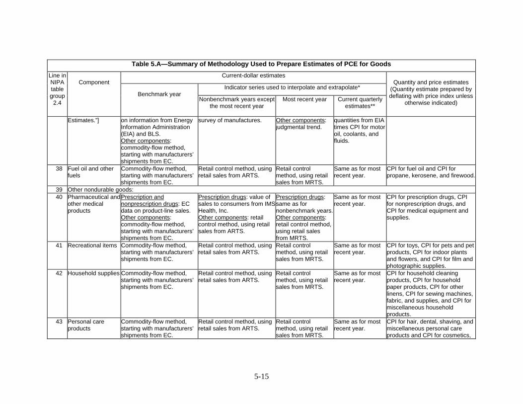
Table 5.A—Summary of Methodology Used to Prepare Estimates of PCE for Goods Current-dollar estimates
Indicator series used to interpolate and extrapolate*
Line in NIPA table group
2.4
Component
Benchmark year
Nonbenchmark years except the most recent year
Most recent year
Current quarterly estimates**
Quantity and price estimates
(Quantity estimate prepared by deflating with price index unless
otherwise indicated)
Estimates.”] on information from Energy Information Administration (EIA) and BLS. Other components: commodity-flow method, starting with manufacturers’ shipments from EC.
survey of manufactures. Other components: judgmental trend.
quantities from EIA times CPI for motor oil, coolants, and fluids.
38 Fuel oil and other fuels
Commodity-flow method, starting with manufacturers’ shipments from EC.
Retail control method, using retail sales from ARTS.
Retail control method, using retail sales from MRTS.
Same as for most recent year.
CPI for fuel oil and CPI for propane, kerosene, and firewood.
39 Other nondurable goods: 40 Pharmaceutical and
other medical products
Prescription and nonprescription drugs: EC data on product-line sales. Other components: commodity-flow method, starting with manufacturers’ shipments from EC.
Prescription drugs: value of sales to consumers from IMSHealth, Inc.
Other components: retail control method, using retail sales from ARTS.
Prescription drugs: same as for nonbenchmark years. Other components: retail control method, using retail sales from MRTS.
Same as for most recent year.
CPI for prescription drugs, CPI for nonprescription drugs, and CPI for medical equipment and supplies.
41 Recreational items Commodity-flow method, starting with manufacturers’ shipments from EC.
Retail control method, using retail sales from ARTS.
Retail control method, using retail sales from MRTS.
Same as for most recent year.
CPI for toys, CPI for pets and pet products, CPI for indoor plants and flowers, and CPI for film and photographic supplies.
42 Household supplies Commodity-flow method, starting with manufacturers’ shipments from EC.
Retail control method, using retail sales from ARTS.
Retail control method, using retail sales from MRTS.
Same as for most recent year.
CPI for household cleaning products, CPI for household paper products, CPI for other linens, CPI for sewing machines, fabric, and supplies, and CPI for miscellaneous household products.
43 Personal care products
Commodity-flow method, starting with manufacturers’ shipments from EC.
Retail control method, using retail sales from ARTS.
Retail control method, using retail sales from MRTS.
Same as for most recent year.
CPI for hair, dental, shaving, and miscellaneous personal care products and CPI for cosmetics,
5-15
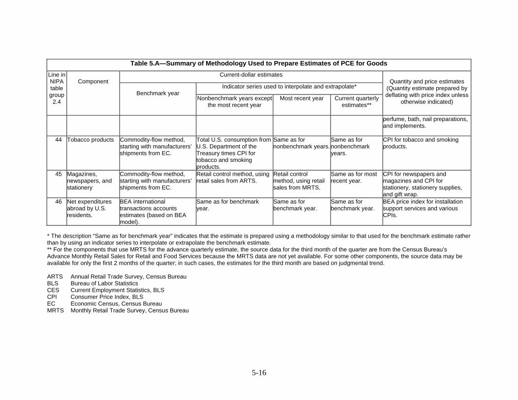
5-16
Table 5.A—Summary of Methodology Used to Prepare Estimates of PCE for Goods Current-dollar estimates
Indicator series used to interpolate and extrapolate*
Line in NIPA table group
2.4
Component
Benchmark year
Nonbenchmark years except the most recent year
Most recent year
Current quarterly estimates**
Quantity and price estimates
(Quantity estimate prepared by deflating with price index unless
otherwise indicated)
perfume, bath, nail preparations, and implements.
44 Tobacco products Commodity-flow method, starting with manufacturers’ shipments from EC.
Total U.S. consumption from U.S. Department of the Treasury times CPI for tobacco and smoking products.
Same as for nonbenchmark years.
Same as for nonbenchmark years.
CPI for tobacco and smoking products.
45 Magazines, newspapers, and stationery
Commodity-flow method, starting with manufacturers’ shipments from EC.
Retail control method, using retail sales from ARTS.
Retail control method, using retail sales from MRTS.
Same as for most recent year.
CPI for newspapers and magazines and CPI for stationery, stationery supplies, and gift wrap.
46 Net expenditures abroad by U.S. residents.
BEA international transactions accounts estimates (based on BEA model).
Same as for benchmark year.
Same as for benchmark year.
Same as for benchmark year.
BEA price index for installation support services and various CPIs.
* The description “Same as for benchmark year” indicates that the estimate is prepared using a methodology similar to that used for the benchmark estimate rather than by using an indicator series to interpolate or extrapolate the benchmark estimate. ** For the components that use MRTS for the advance quarterly estimate, the source data for the third month of the quarter are from the Census Bureau’s Advance Monthly Retail Sales for Retail and Food Services because the MRTS data are not yet available. For some other components, the source data may be available for only the first 2 months of the quarter; in such cases, the estimates for the third month are based on judgmental trend. ARTS Annual Retail Trade Survey, Census Bureau BLS Bureau of Labor Statistics CES Current Employment Statistics, BLS CPI Consumer Price Index, BLS EC Economic Census, Census Bureau MRTS Monthly Retail Trade Survey, Census Bureau
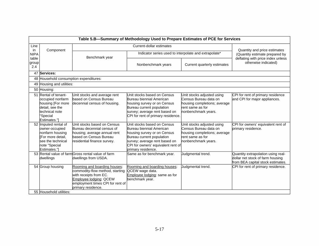
Table 5.B—Summary of Methodology Used to Prepare Estimates of PCE for Services Current-dollar estimates
Indicator series used to interpolate and extrapolate*
Line in
NIPA table group
2.4
Component
Benchmark year
Nonbenchmark years
Current quarterly estimates
Quantity and price estimates
(Quantity estimate prepared by deflating with price index unless
otherwise indicated)
47 Services: 48 Household consumption expenditures: 49 Housing and utilities: 50 Housing: 51 Rental of tenant-
occupied nonfarm housing [For more detail, see the technical note “Special Estimates.”]
Unit stocks and average rent based on Census Bureau decennial census of housing.
Unit stocks based on Census Bureau biennial American housing survey or on Census Bureau current population survey; average rent based on CPI for rent of primary residence.
Unit stocks adjusted using Census Bureau data on housing completions; average rent same as for nonbenchmark years.
CPI for rent of primary residence and CPI for major appliances.
52 Imputed rental of owner-occupied nonfarm housing [For more detail, see the technical note “Special Estimates.”]
Unit stocks based on Census Bureau decennial census of housing; average annual rent based on Census Bureau residential finance survey.
Unit stocks based on Census Bureau biennial American housing survey or on Census Bureau current population survey; average rent based on CPI for owners’ equivalent rent of primary residence.
Unit stocks adjusted using Census Bureau data on housing completions; average rent same as for nonbenchmark years.
CPI for owners’ equivalent rent of primary residence.
53 Rental value of farm dwellings
Gross rental value of farm dwellings from USDA.
Same as for benchmark year. Judgmental trend.
Quantity extrapolation using real-dollar net stock of farm housing from BEA capital stock estimates.
54 Group housing Rooming and boarding houses: commodity-flow method, starting with receipts from EC. Employee lodging: QCEW employment times CPI for rent of primary residence.
Rooming and boarding houses: QCEW wage data. Employee lodging: same as for benchmark year.
Judgmental trend.
CPI for rent of primary residence.
55 Household utilities:
5-17
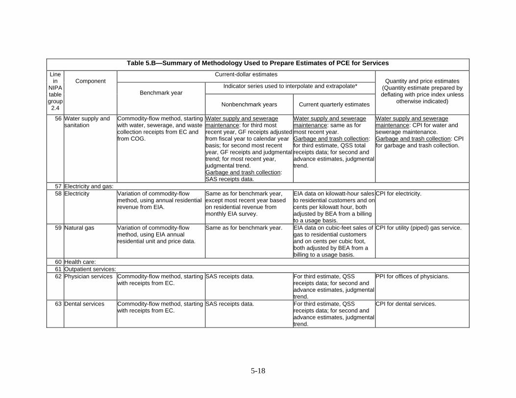
Table 5.B—Summary of Methodology Used to Prepare Estimates of PCE for Services Current-dollar estimates
Indicator series used to interpolate and extrapolate*
Line in
NIPA table group
2.4
Component
Benchmark year
Nonbenchmark years
Current quarterly estimates
Quantity and price estimates
(Quantity estimate prepared by deflating with price index unless
otherwise indicated)
56 Water supply and sanitation
Commodity-flow method, starting with water, sewerage, and waste collection receipts from EC and from COG.
Water supply and sewerage maintenance: for third most recent year, GF receipts adjusted from fiscal year to calendar year basis; for second most recent year, GF receipts and judgmental trend; for most recent year, judgmental trend. Garbage and trash collection: SAS receipts data.
Water supply and sewerage maintenance: same as for most recent year. Garbage and trash collection: for third estimate, QSS total receipts data; for second and advance estimates, judgmental trend.
Water supply and sewerage maintenance: CPI for water and sewerage maintenance. Garbage and trash collection: CPI for garbage and trash collection.
57 Electricity and gas: 58 Electricity Variation of commodity-flow
method, using annual residential revenue from EIA.
Same as for benchmark year, except most recent year based on residential revenue from monthly EIA survey.
EIA data on kilowatt-hour sales to residential customers and on cents per kilowatt hour, both adjusted by BEA from a billing to a usage basis.
CPI for electricity.
59 Natural gas
Variation of commodity-flow method, using EIA annual residential unit and price data.
Same as for benchmark year. EIA data on cubic-feet sales of gas to residential customers and on cents per cubic foot, both adjusted by BEA from a billing to a usage basis.
CPI for utility (piped) gas service.
60 Health care: 61 Outpatient services: 62 Physician services Commodity-flow method, starting
with receipts from EC. SAS receipts data. For third estimate, QSS
receipts data; for second and advance estimates, judgmental trend.
PPI for offices of physicians.
63 Dental services Commodity-flow method, starting with receipts from EC.
SAS receipts data. For third estimate, QSS receipts data; for second and advance estimates, judgmental trend.
CPI for dental services.
5-18
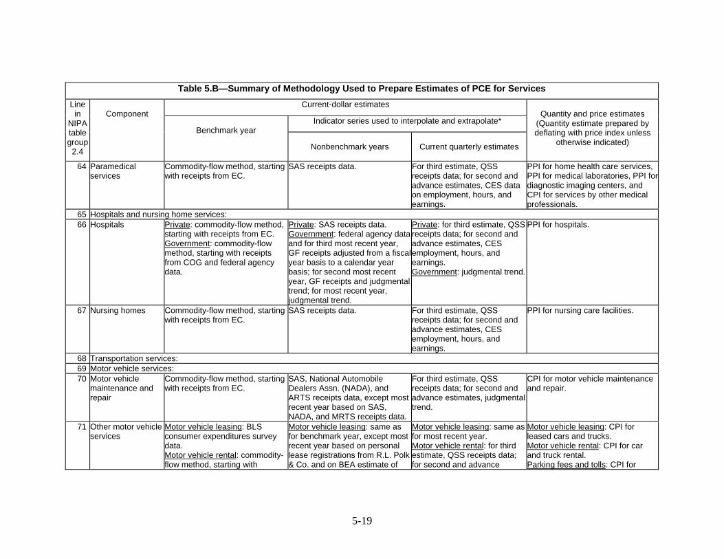
Table 5.B—Summary of Methodology Used to Prepare Estimates of PCE for Services Current-dollar estimates
Indicator series used to interpolate and extrapolate*
Line in
NIPA table group
2.4
Component
Benchmark year
Nonbenchmark years
Current quarterly estimates
Quantity and price estimates
(Quantity estimate prepared by deflating with price index unless
otherwise indicated)
64 Paramedical services
Commodity-flow method, starting with receipts from EC.
SAS receipts data. For third estimate, QSS receipts data; for second and advance estimates, CES data on employment, hours, and earnings.
PPI for home health care services, PPI for medical laboratories, PPI for diagnostic imaging centers, and CPI for services by other medical professionals.
65 Hospitals and nursing home services: 66 Hospitals Private: commodity-flow method,
starting with receipts from EC. Government: commodity-flow method, starting with receipts from COG and federal agency data.
Private: SAS receipts data. Government: federal agency data and for third most recent year, GF receipts adjusted from a fiscal year basis to a calendar year basis; for second most recent year, GF receipts and judgmental trend; for most recent year, judgmental trend.
Private: for third estimate, QSS receipts data; for second and advance estimates, CES employment, hours, and earnings. Government: judgmental trend.
PPI for hospitals.
67 Nursing homes Commodity-flow method, starting with receipts from EC.
SAS receipts data. For third estimate, QSS receipts data; for second and advance estimates, CES employment, hours, and earnings.
PPI for nursing care facilities.
68 Transportation services: 69 Motor vehicle services: 70 Motor vehicle
maintenance and repair
Commodity-flow method, starting with receipts from EC.
SAS, National Automobile Dealers Assn. (NADA), and ARTS receipts data, except most recent year based on SAS, NADA, and MRTS receipts data.
For third estimate, QSS receipts data; for second and advance estimates, judgmental trend.
CPI for motor vehicle maintenance and repair.
71 Other motor vehicle services
Motor vehicle leasing: BLS consumer expenditures survey data. Motor vehicle rental: commodity-flow method, starting with
Motor vehicle leasing: same as for benchmark year, except most recent year based on personal lease registrations from R.L. Polk & Co. and on BEA estimate of
Motor vehicle leasing: same as for most recent year. Motor vehicle rental: for third estimate, QSS receipts data; for second and advance
Motor vehicle leasing: CPI for leased cars and trucks. Motor vehicle rental: CPI for car and truck rental. Parking fees and tolls: CPI for
5-19
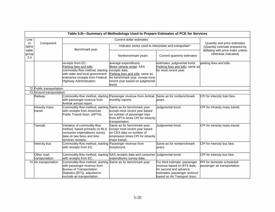
Table 5.B—Summary of Methodology Used to Prepare Estimates of PCE for Services Current-dollar estimates
Indicator series used to interpolate and extrapolate*
Line in
NIPA table group
2.4
Component
Benchmark year
Nonbenchmark years
Current quarterly estimates
Quantity and price estimates
(Quantity estimate prepared by deflating with price index unless
otherwise indicated)
receipts from EC. Parking fees and tolls: commodity-flow method, starting with state and local government enterprise receipts from Federal Highway Administration.
average expenditures. Motor vehicle rental: SAS receipts data. Parking fees and tolls: same as for benchmark year, except most recent year based on judgmental trend.
estimates, judgmental trend. Parking fees and tolls: same as for most recent year.
parking fees and tolls.
72 Public transportation: 73 Ground transportation: Railway Commodity-flow method, starting
with passenger revenue from Amtrak annual report.
Passenger revenue from Amtrak monthly reports.
Same as for nonbenchmark years.
CPI for intercity train fare.
Intracity mass transit
Commodity-flow method, starting with receipts from American Public Transit Assn. (APTA).
Same as for benchmark year, except most recent year based on number of passenger trips from APTA times CPI for intracity transportation.
Judgmental trend.
CPI for intracity mass transit.
Taxicab Variation of commodity-flow method, based primarily on BLS consumer expenditures survey data on taxi fares and limo services receipts.
Same as for benchmark year, except most recent year based on CES data on number of employees times CPI for intracity mass transit.
Judgmental trend.
CPI for intracity mass transit.
Intercity bus Commodity-flow method, starting with receipts from EC.
Passenger revenue from Greyhound.
Same as for nonbenchmark years.
CPI for intercity bus fare.
Other road transportation
Commodity-flow method, starting with receipts from EC.
SAS receipts data and consumer expenditures survey data.
Judgmental trend. CPI for intercity bus fare.
74 Air transportation Commodity-flow method, starting with passenger revenue from Bureau of Transportation Statistics (BTS), adjusted to exclude air transportation
Same as for benchmark year. For third estimate, passenger revenue based on BTS data; for second and advance estimates, passenger revenue based on Air Transport Assn.
PPI for domestic scheduled passenger air transportation.
5-20
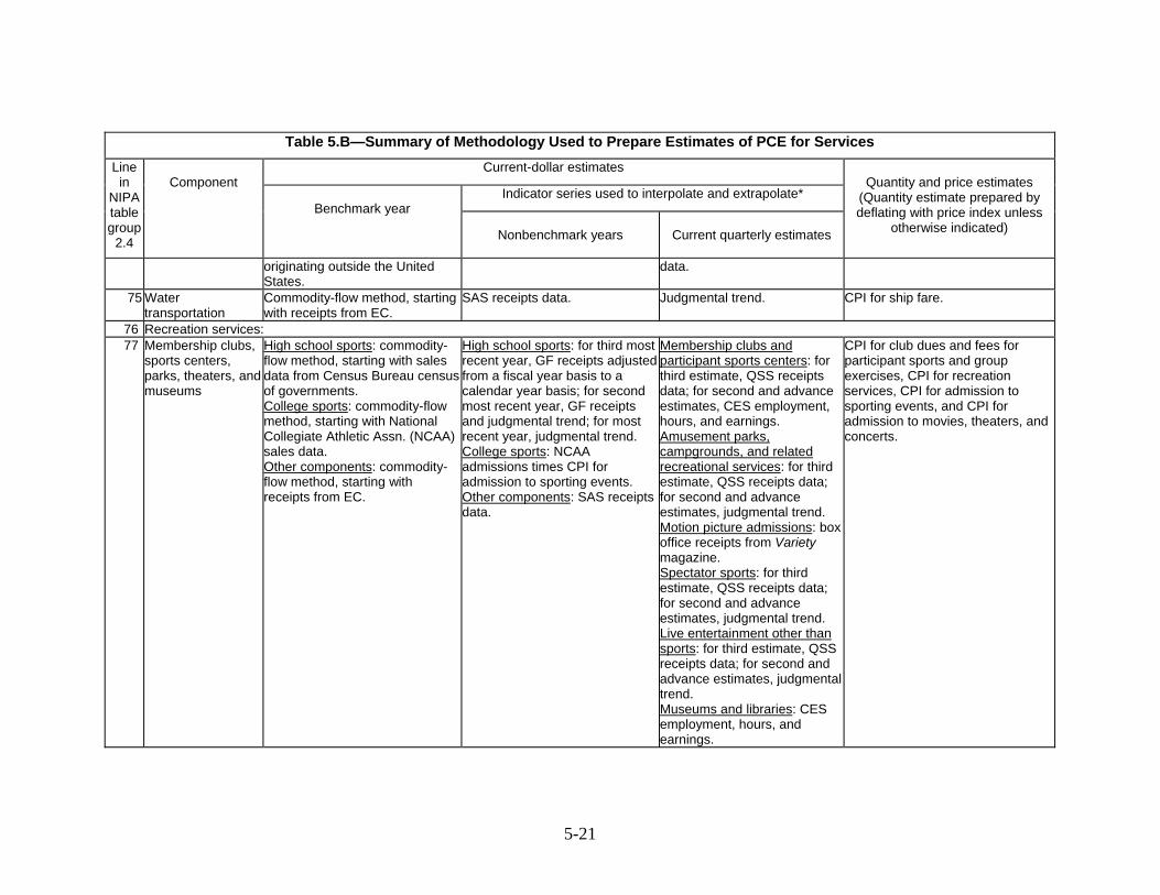
Table 5.B—Summary of Methodology Used to Prepare Estimates of PCE for Services Current-dollar estimates
Indicator series used to interpolate and extrapolate*
Line in
NIPA table group
2.4
Component
Benchmark year
Nonbenchmark years
Current quarterly estimates
Quantity and price estimates
(Quantity estimate prepared by deflating with price index unless
otherwise indicated)
originating outside the United States.
data.
75 Water transportation
Commodity-flow method, starting with receipts from EC.
SAS receipts data. Judgmental trend. CPI for ship fare.
76 Recreation services: 77 Membership clubs,
sports centers, parks, theaters, and museums
High school sports: commodity-flow method, starting with sales data from Census Bureau census of governments. College sports: commodity-flow method, starting with National Collegiate Athletic Assn. (NCAA) sales data. Other components: commodity-flow method, starting with receipts from EC.
High school sports: for third most recent year, GF receipts adjusted from a fiscal year basis to a calendar year basis; for second most recent year, GF receipts and judgmental trend; for most recent year, judgmental trend. College sports: NCAA admissions times CPI for admission to sporting events. Other components: SAS receipts data.
Membership clubs and participant sports centers: for third estimate, QSS receipts data; for second and advance estimates, CES employment, hours, and earnings. Amusement parks, campgrounds, and related recreational services: for third estimate, QSS receipts data; for second and advance estimates, judgmental trend. Motion picture admissions: box office receipts from Variety magazine. Spectator sports: for third estimate, QSS receipts data; for second and advance estimates, judgmental trend. Live entertainment other than sports: for third estimate, QSS receipts data; for second and advance estimates, judgmental trend. Museums and libraries: CES employment, hours, and earnings.
CPI for club dues and fees for participant sports and group exercises, CPI for recreation services, CPI for admission to sporting events, and CPI for admission to movies, theaters, and concerts.
5-21
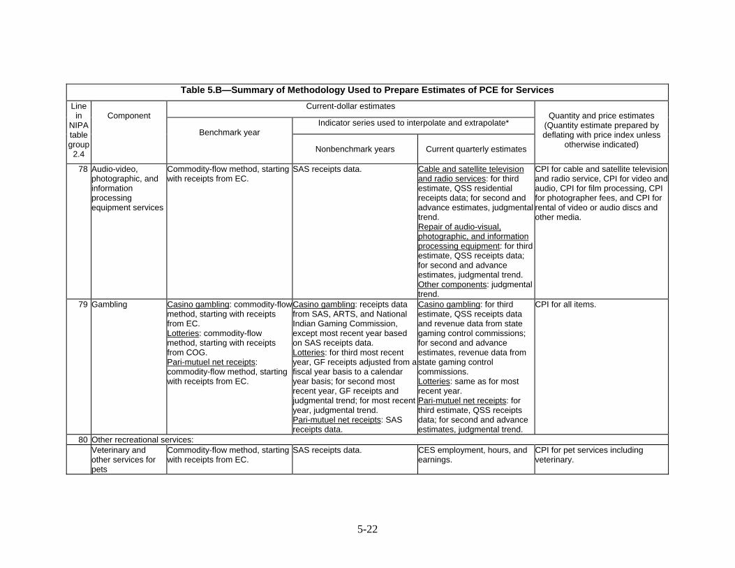
Table 5.B—Summary of Methodology Used to Prepare Estimates of PCE for Services Current-dollar estimates
Indicator series used to interpolate and extrapolate*
Line in
NIPA table group
2.4
Component
Benchmark year
Nonbenchmark years
Current quarterly estimates
Quantity and price estimates
(Quantity estimate prepared by deflating with price index unless
otherwise indicated)
78 Audio-video, photographic, and information processing equipment services
Commodity-flow method, starting with receipts from EC.
SAS receipts data. Cable and satellite television and radio services: for third estimate, QSS residential receipts data; for second and advance estimates, judgmental trend. Repair of audio-visual, photographic, and information processing equipment: for third estimate, QSS receipts data; for second and advance estimates, judgmental trend. Other components: judgmental trend.
CPI for cable and satellite television and radio service, CPI for video and audio, CPI for film processing, CPI for photographer fees, and CPI for rental of video or audio discs and other media.
79 Gambling Casino gambling: commodity-flowmethod, starting with receipts from EC.
Lotteries: commodity-flow method, starting with receipts from COG. Pari-mutuel net receipts: commodity-flow method, starting with receipts from EC.
Casino gambling: receipts data from SAS, ARTS, and National Indian Gaming Commission, except most recent year based on SAS receipts data. Lotteries: for third most recent year, GF receipts adjusted from a fiscal year basis to a calendar year basis; for second most recent year, GF receipts and judgmental trend; for most recent year, judgmental trend. Pari-mutuel net receipts: SAS receipts data.
Casino gambling: for third estimate, QSS receipts data and revenue data from state gaming control commissions; for second and advance estimates, revenue data from state gaming control commissions. Lotteries: same as for most recent year. Pari-mutuel net receipts: for third estimate, QSS receipts data; for second and advance estimates, judgmental trend.
CPI for all items.
80 Other recreational services: Veterinary and
other services for pets
Commodity-flow method, starting with receipts from EC.
SAS receipts data. CES employment, hours, and earnings.
CPI for pet services including veterinary.
5-22
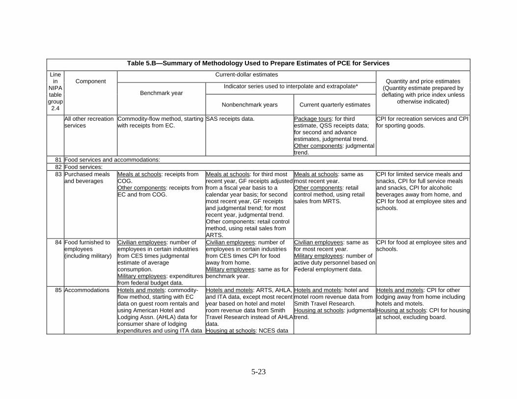
Table 5.B—Summary of Methodology Used to Prepare Estimates of PCE for Services Current-dollar estimates
Indicator series used to interpolate and extrapolate*
Line in
NIPA table group
2.4
Component
Benchmark year
Nonbenchmark years
Current quarterly estimates
Quantity and price estimates
(Quantity estimate prepared by deflating with price index unless
otherwise indicated)
All other recreation services
Commodity-flow method, starting with receipts from EC.
SAS receipts data. Package tours: for third estimate, QSS receipts data; for second and advance estimates, judgmental trend. Other components: judgmental trend.
CPI for recreation services and CPI for sporting goods.
81 Food services and accommodations: 82 Food services: 83 Purchased meals
and beverages Meals at schools: receipts from COG. Other components: receipts from EC and from COG.
Meals at schools: for third most recent year, GF receipts adjusted from a fiscal year basis to a calendar year basis; for second most recent year, GF receipts and judgmental trend; for most recent year, judgmental trend. Other components: retail control method, using retail sales from ARTS.
Meals at schools: same as most recent year. Other components: retail control method, using retail sales from MRTS.
CPI for limited service meals and snacks, CPI for full service meals and snacks, CPI for alcoholic beverages away from home, and CPI for food at employee sites and schools.
84 Food furnished to employees (including military)
Civilian employees: number of employees in certain industries from CES times judgmental estimate of average consumption. Military employees: expenditures from federal budget data.
Civilian employees: number of employees in certain industries from CES times CPI for food away from home. Military employees: same as for benchmark year.
Civilian employees: same as for most recent year. Military employees: number of active duty personnel based on Federal employment data.
CPI for food at employee sites and schools.
85 Accommodations Hotels and motels: commodity-flow method, starting with EC data on guest room rentals and using American Hotel and Lodging Assn. (AHLA) data for consumer share of lodging expenditures and using ITA data
Hotels and motels: ARTS, AHLA, and ITA data, except most recent year based on hotel and motel room revenue data from Smith Travel Research instead of AHLA data. Housing at schools: NCES data
Hotels and motels: hotel and motel room revenue data from Smith Travel Research. Housing at schools: judgmental trend.
Hotels and motels: CPI for other lodging away from home including hotels and motels. Housing at schools: CPI for housing at school, excluding board.
5-23
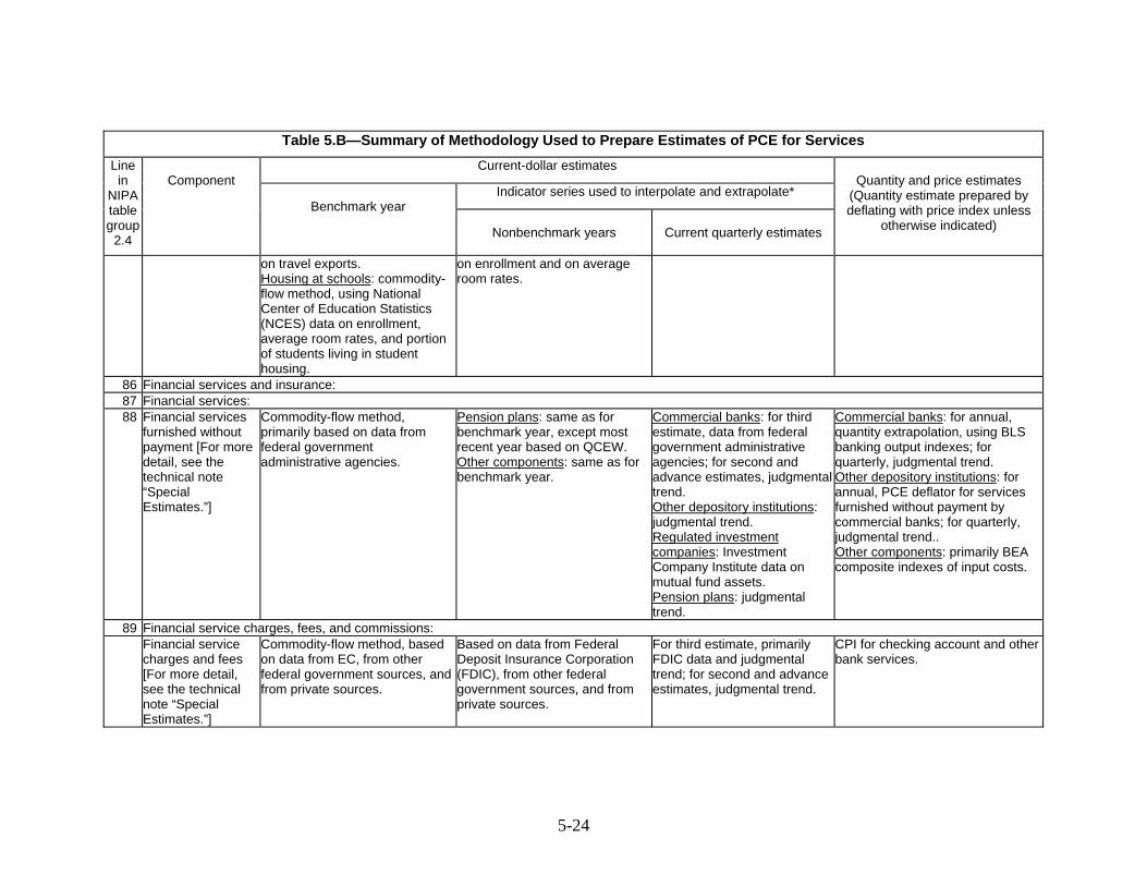
Table 5.B—Summary of Methodology Used to Prepare Estimates of PCE for Services Current-dollar estimates
Indicator series used to interpolate and extrapolate*
Line in
NIPA table group
2.4
Component
Benchmark year
Nonbenchmark years
Current quarterly estimates
Quantity and price estimates
(Quantity estimate prepared by deflating with price index unless
otherwise indicated)
on travel exports. Housing at schools: commodity-flow method, using National Center of Education Statistics (NCES) data on enrollment, average room rates, and portion of students living in student housing.
on enrollment and on average room rates.
86 Financial services and insurance: 87 Financial services: 88 Financial services
furnished without payment [For more detail, see the technical note “Special Estimates.”]
Commodity-flow method, primarily based on data from federal government administrative agencies.
Pension plans: same as for benchmark year, except most recent year based on QCEW. Other components: same as for benchmark year.
Commercial banks: for third estimate, data from federal government administrative agencies; for second and advance estimates, judgmental trend. Other depository institutions: judgmental trend. Regulated investment companies: Investment Company Institute data on mutual fund assets. Pension plans: judgmental trend.
Commercial banks: for annual, quantity extrapolation, using BLS banking output indexes; for quarterly, judgmental trend. Other depository institutions: for annual, PCE deflator for services furnished without payment by commercial banks; for quarterly, judgmental trend.. Other components: primarily BEA composite indexes of input costs.
89 Financial service charges, fees, and commissions: Financial service
charges and fees [For more detail, see the technical note “Special Estimates.”]
Commodity-flow method, based on data from EC, from other federal government sources, and from private sources.
Based on data from Federal Deposit Insurance Corporation (FDIC), from other federal government sources, and from private sources.
For third estimate, primarily FDIC data and judgmental trend; for second and advance estimates, judgmental trend.
CPI for checking account and other bank services.
5-24
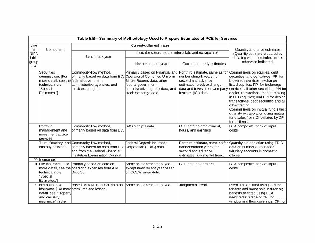
Table 5.B—Summary of Methodology Used to Prepare Estimates of PCE for Services Current-dollar estimates
Indicator series used to interpolate and extrapolate*
Line in
NIPA table group
2.4
Component
Benchmark year
Nonbenchmark years
Current quarterly estimates
Quantity and price estimates
(Quantity estimate prepared by deflating with price index unless
otherwise indicated)
Securities commissions [For more detail, see the technical note “Special Estimates.”]
Commodity-flow method, primarily based on data from EC, federal government administrative agencies, and stock exchanges.
Primarily based on Financial and Operational Combined Uniform Single Reports data, other federal government administrative agency data, and stock exchange data.
For third estimate, same as for nonbenchmark years; for second and advance estimates, stock exchange data and Investment Company Institute (ICI) data.
Commissions on equities, debt securities, and derivatives: PPI for brokerage services, exchange listed equities; PPI for brokerage services, all other securities; PPI for dealer transactions, market-making in OTC equities; and PPI for dealer transactions, debt securities and all other trading. Commissions on mutual fund sales: quantity extrapolation using mutual fund sales from ICI deflated by CPI for all items.
Portfolio management and investment advice services
Commodity-flow method, primarily based on data from EC.
SAS receipts data. CES data on employment, hours, and earnings.
BEA composite index of input costs.
Trust, fiduciary, and custody activities
Commodity-flow method, primarily based on data from EC and from the Federal Financial Institution Examination Council.
Federal Deposit Insurance Corporation (FDIC) data.
For third estimate, same as for nonbenchmark years; for second and advance estimates, judgmental trend.
Quantity extrapolation using FDIC data on number of managed fiduciary accounts in domestic offices.
90 Insurance: 91 Life insurance [For
more detail, see the technical note “Special Estimates.”]
Primarily based on data on operating expenses from A.M. Best Co.
Same as for benchmark year, except most recent year based on QCEW wage data.
CES data on earnings. BEA composite index of input costs.
92 Net household insurance [For more detail, see “Propertyand casualty insurance” in the
Based on A.M. Best Co. data on premiums and losses.
Same as for benchmark year. Judgmental trend. Premiums deflated using CPI for tenants and household insurance; benefits deflated using BEA weighted average of CPI for window and floor coverings, CPI for
5-25
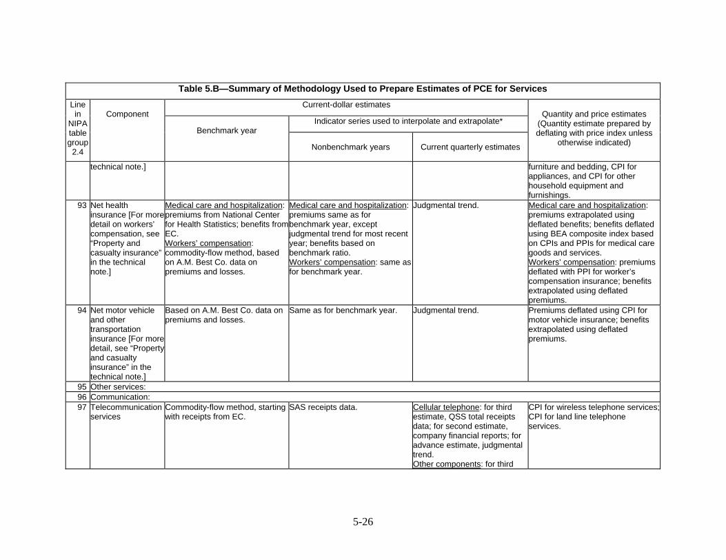
Table 5.B—Summary of Methodology Used to Prepare Estimates of PCE for Services Current-dollar estimates
Indicator series used to interpolate and extrapolate*
Line in
NIPA table group
2.4
Component
Benchmark year
Nonbenchmark years
Current quarterly estimates
Quantity and price estimates
(Quantity estimate prepared by deflating with price index unless
otherwise indicated)
technical note.] furniture and bedding, CPI for appliances, and CPI for other household equipment and furnishings.
93 Net health insurance [For more detail on workers’ compensation, see “Property and casualty insurance” in the technical note.]
Medical care and hospitalization: premiums from National Center for Health Statistics; benefits fromEC.
Workers’ compensation: commodity-flow method, based on A.M. Best Co. data on premiums and losses.
Medical care and hospitalization: premiums same as for benchmark year, except judgmental trend for most recent year; benefits based on benchmark ratio. Workers’ compensation: same as for benchmark year.
Judgmental trend. Medical care and hospitalization: premiums extrapolated using deflated benefits; benefits deflated using BEA composite index based on CPIs and PPIs for medical care goods and services. Workers’ compensation: premiums deflated with PPI for worker’s compensation insurance; benefits extrapolated using deflated premiums.
94 Net motor vehicle and other transportation insurance [For more detail, see “Property and casualty insurance” in the technical note.]
Based on A.M. Best Co. data on premiums and losses.
Same as for benchmark year. Judgmental trend. Premiums deflated using CPI for motor vehicle insurance; benefits extrapolated using deflated premiums.
95 Other services: 96 Communication: 97 Telecommunication
services Commodity-flow method, starting with receipts from EC.
SAS receipts data. Cellular telephone: for third estimate, QSS total receipts data; for second estimate, company financial reports; for advance estimate, judgmental trend. Other components: for third
CPI for wireless telephone services;CPI for land line telephone services.
5-26
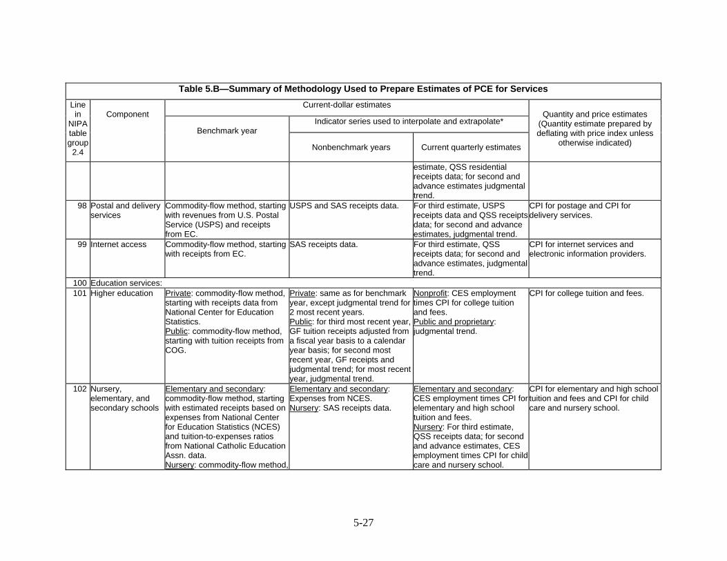
Table 5.B—Summary of Methodology Used to Prepare Estimates of PCE for Services Current-dollar estimates
Indicator series used to interpolate and extrapolate*
Line in
NIPA table group
2.4
Component
Benchmark year
Nonbenchmark years
Current quarterly estimates
Quantity and price estimates
(Quantity estimate prepared by deflating with price index unless
otherwise indicated)
estimate, QSS residential receipts data; for second and advance estimates judgmental trend.
98 Postal and delivery services
Commodity-flow method, starting with revenues from U.S. Postal Service (USPS) and receipts from EC.
USPS and SAS receipts data. For third estimate, USPS receipts data and QSS receipts data; for second and advance estimates, judgmental trend.
CPI for postage and CPI for delivery services.
99 Internet access Commodity-flow method, starting with receipts from EC.
SAS receipts data. For third estimate, QSS receipts data; for second and advance estimates, judgmental trend.
CPI for internet services and electronic information providers.
100 Education services: 101 Higher education Private: commodity-flow method,
starting with receipts data from National Center for Education Statistics. Public: commodity-flow method, starting with tuition receipts from COG.
Private: same as for benchmark year, except judgmental trend for 2 most recent years. Public: for third most recent year, GF tuition receipts adjusted from a fiscal year basis to a calendar year basis; for second most recent year, GF receipts and judgmental trend; for most recent year, judgmental trend.
Nonprofit: CES employment times CPI for college tuition and fees. Public and proprietary: judgmental trend.
CPI for college tuition and fees.
102 Nursery, elementary, and secondary schools
Elementary and secondary: commodity-flow method, starting with estimated receipts based on expenses from National Center for Education Statistics (NCES) and tuition-to-expenses ratios from National Catholic Education Assn. data. Nursery: commodity-flow method,
Elementary and secondary: Expenses from NCES. Nursery: SAS receipts data.
Elementary and secondary: CES employment times CPI for elementary and high school tuition and fees. Nursery: For third estimate, QSS receipts data; for second and advance estimates, CES employment times CPI for child care and nursery school.
CPI for elementary and high school tuition and fees and CPI for child care and nursery school.
5-27
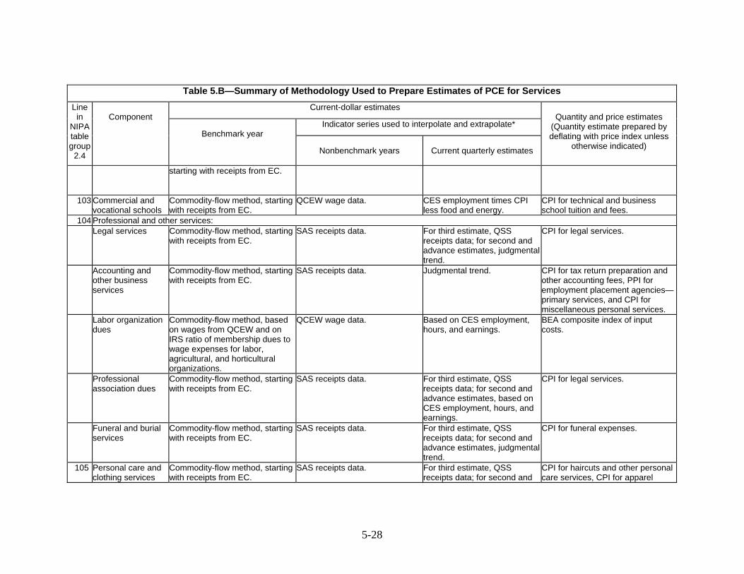
Table 5.B—Summary of Methodology Used to Prepare Estimates of PCE for Services Current-dollar estimates
Indicator series used to interpolate and extrapolate*
Line in
NIPA table group
2.4
Component
Benchmark year
Nonbenchmark years
Current quarterly estimates
Quantity and price estimates
(Quantity estimate prepared by deflating with price index unless
otherwise indicated)
starting with receipts from EC.
103 Commercial and vocational schools
Commodity-flow method, starting with receipts from EC.
QCEW wage data. CES employment times CPI less food and energy.
CPI for technical and business school tuition and fees.
104 Professional and other services: Legal services Commodity-flow method, starting
with receipts from EC. SAS receipts data. For third estimate, QSS
receipts data; for second and advance estimates, judgmental trend.
CPI for legal services.
Accounting and other business services
Commodity-flow method, starting with receipts from EC.
SAS receipts data. Judgmental trend. CPI for tax return preparation and other accounting fees, PPI for employment placement agencies—primary services, and CPI for miscellaneous personal services.
Labor organization dues
Commodity-flow method, based on wages from QCEW and on IRS ratio of membership dues to wage expenses for labor, agricultural, and horticultural organizations.
QCEW wage data. Based on CES employment, hours, and earnings.
BEA composite index of input costs.
Professional association dues
Commodity-flow method, starting with receipts from EC.
SAS receipts data. For third estimate, QSS receipts data; for second and advance estimates, based on CES employment, hours, and earnings.
CPI for legal services.
Funeral and burial services
Commodity-flow method, starting with receipts from EC.
SAS receipts data. For third estimate, QSS receipts data; for second and advance estimates, judgmental trend.
CPI for funeral expenses.
105 Personal care and clothing services
Commodity-flow method, starting with receipts from EC.
SAS receipts data. For third estimate, QSS receipts data; for second and
CPI for haircuts and other personal care services, CPI for apparel
5-28
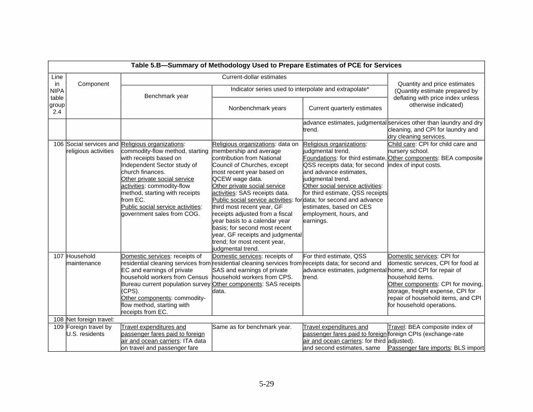
Table 5.B—Summary of Methodology Used to Prepare Estimates of PCE for Services Current-dollar estimates
Indicator series used to interpolate and extrapolate*
Line in
NIPA table group
2.4
Component
Benchmark year
Nonbenchmark years
Current quarterly estimates
Quantity and price estimates
(Quantity estimate prepared by deflating with price index unless
otherwise indicated)
advance estimates, judgmental trend.
services other than laundry and dry cleaning, and CPI for laundry and dry cleaning services.
106 Social services and religious activities
Religious organizations: commodity-flow method, starting with receipts based on Independent Sector study of church finances. Other private social service activities: commodity-flow method, starting with receipts from EC. Public social service activities: government sales from COG.
Religious organizations: data on membership and average contribution from National Council of Churches, except most recent year based on QCEW wage data. Other private social service activities: SAS receipts data. Public social service activities: for third most recent year, GF receipts adjusted from a fiscal year basis to a calendar year basis; for second most recent year, GF receipts and judgmental trend; for most recent year, judgmental trend.
Religious organizations: judgmental trend. Foundations: for third estimate, QSS receipts data; for second and advance estimates, judgmental trend. Other social service activities: for third estimate, QSS receipts data; for second and advance estimates, based on CES employment, hours, and earnings.
Child care: CPI for child care and nursery school. Other components: BEA composite index of input costs.
107 Household maintenance
Domestic services: receipts of residential cleaning services from EC and earnings of private household workers from Census Bureau current population survey (CPS). Other components: commodity-flow method, starting with receipts from EC.
Domestic services: receipts of residential cleaning services from SAS and earnings of private household workers from CPS. Other components: SAS receipts data.
For third estimate, QSS receipts data; for second and advance estimates, judgmental trend.
Domestic services: CPI for domestic services, CPI for food at home, and CPI for repair of household items. Other components: CPI for moving, storage, freight expense, CPI for repair of household items, and CPI for household operations.
108 Net foreign travel: 109 Foreign travel by
U.S. residents Travel expenditures and passenger fares paid to foreign air and ocean carriers: ITA data on travel and passenger fare
Same as for benchmark year. Travel expenditures and passenger fares paid to foreign air and ocean carriers: for third and second estimates, same
Travel: BEA composite index of foreign CPIs (exchange-rate adjusted). Passenger fare imports: BLS import
5-29
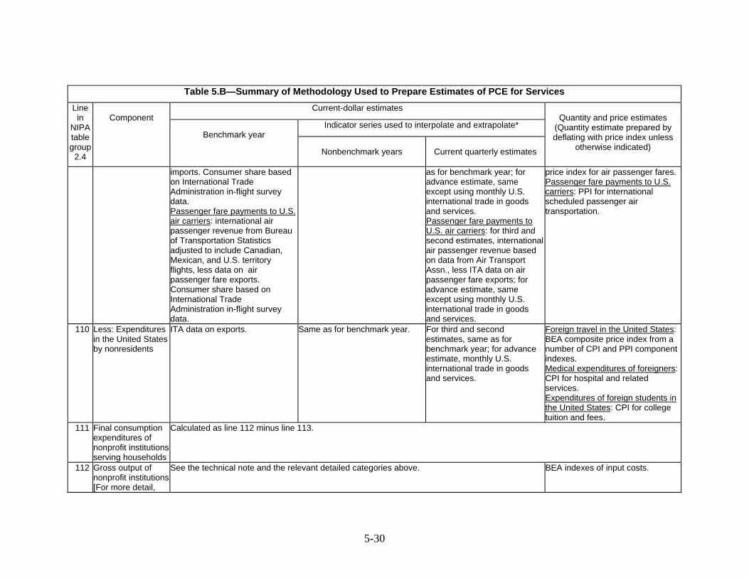
Table 5.B—Summary of Methodology Used to Prepare Estimates of PCE for Services Current-dollar estimates
Indicator series used to interpolate and extrapolate*
Line in
NIPA table group
2.4
Component
Benchmark year
Nonbenchmark years
Current quarterly estimates
Quantity and price estimates
(Quantity estimate prepared by deflating with price index unless
otherwise indicated)
imports. Consumer share based on International Trade Administration in-flight survey data. Passenger fare payments to U.S. air carriers: international air passenger revenue from Bureau of Transportation Statistics adjusted to include Canadian, Mexican, and U.S. territory flights, less data on air passenger fare exports. Consumer share based on International Trade Administration in-flight survey data.
as for benchmark year; for advance estimate, same except using monthly U.S. international trade in goods and services. Passenger fare payments to U.S. air carriers: for third and second estimates, international air passenger revenue based on data from Air Transport Assn., less ITA data on air passenger fare exports; for advance estimate, same except using monthly U.S. international trade in goods and services.
price index for air passenger fares.Passenger fare payments to U.S. carriers: PPI for international scheduled passenger air transportation.
110 Less: Expenditures in the United States by nonresidents
ITA data on exports. Same as for benchmark year. For third and second estimates, same as for benchmark year; for advance estimate, monthly U.S. international trade in goods and services.
Foreign travel in the United States:BEA composite price index from a number of CPI and PPI component indexes. Medical expenditures of foreigners:CPI for hospital and related services. Expenditures of foreign students in the United States: CPI for college tuition and fees.
111 Final consumption expenditures of nonprofit institutions serving households
Calculated as line 112 minus line 113.
112 Gross output of nonprofit institutions [For more detail,
See the technical note and the relevant detailed categories above. BEA indexes of input costs.
5-30

5-31
Table 5.B—Summary of Methodology Used to Prepare Estimates of PCE for Services Current-dollar estimates
Indicator series used to interpolate and extrapolate*
Line in
NIPA table group
2.4
Component
Benchmark year
Nonbenchmark years
Current quarterly estimates
Quantity and price estimates
(Quantity estimate prepared by deflating with price index unless
otherwise indicated)
see technical note “Special Estimates.”]
113 Less: Receipts from sales of goods and services by nonprofit institutions [For more detail, see technical note “Special Estimates.”]
See the technical note and the relevant detailed categories above. See relevant detailed categories above.
* The description “Same as for benchmark” indicates that the estimates are prepared using a methodology similar to that used for the benchmark estimates rather than by using an indicator series to interpolate or extrapolate the benchmark or annual estimates. ARTS Annual Retail Trade Survey, Census Bureau BEA Bureau of Economic Analysis BLS Bureau of Labor Statistics CES Current Employment Statistics, BLS COG Census of Governments, Census Bureau CPI Consumer Price Index, BLS EC Economic Census, Census Bureau EIA Energy Information Administration GF Annual Survey of Government Finances, Census Bureau IRS Internal Revenue Service ITA International Transactions Accounts, BEA MRTS Monthly Retail Trade Survey, Census Bureau PPI Producer Price Index, BLS QCEW Quarterly Census of Employment and Wages, BLS QSS Quarterly Services Survey, Census Bureau SAS Service Annual Survey, Census Bureau USDA U.S. Department of Agriculture
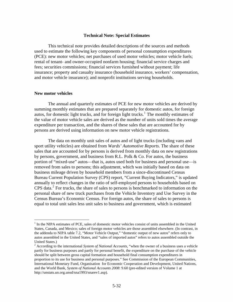
Technical Note: Special Estimates
This technical note provides detailed descriptions of the sources and methods
used to estimate the following key components of personal consumption expenditures (PCE): new motor vehicles; net purchases of used motor vehicles; motor vehicle fuels; rental of tenant- and owner-occupied nonfarm housing; financial service charges and fees; securities commissions; financial services furnished without payment; life insurance; property and casualty insurance (household insurance, workers’ compensation, and motor vehicle insurance); and nonprofit institutions serving households.
New motor vehicles
The annual and quarterly estimates of PCE for new motor vehicles are derived by summing monthly estimates that are prepared separately for domestic autos, for foreign autos, for domestic light trucks, and for foreign light trucks.1 The monthly estimates of the value of motor vehicle sales are derived as the number of units sold times the average expenditure per transaction, and the shares of these sales that are accounted for by persons are derived using information on new motor vehicle registrations.
The data on monthly unit sales of autos and of light trucks (including vans and
sport utility vehicles) are obtained from Wards’ Automotive Reports. The share of these sales that are accounted for by persons is derived from monthly data on new registrations by persons, government, and business from R.L. Polk & Co. For autos, the business portion of “mixed-use” autos—that is, autos used both for business and personal use—is removed from sales to persons; this adjustment, which was initially based on data on business mileage driven by household members from a since-discontinued Census Bureau Current Population Survey (CPS) report, “Current Buying Indicators,” is updated annually to reflect changes in the ratio of self-employed persons to households based on CPS data.2 For trucks, the share of sales to persons is benchmarked to information on the personal share of new truck purchases from the Vehicle Inventory and Use Survey in the Census Bureau’s Economic Census. For foreign autos, the share of sales to persons is equal to total unit sales less unit sales to business and government, which is estimated
1 In the NIPA estimates of PCE, sales of domestic motor vehicles consist of units assembled in the United States, Canada, and Mexico; sales of foreign motor vehicles are those assembled elsewhere. (In contrast, in the addenda to NIPA table 7.2, “Motor Vehicle Output,” “domestic output of new autos” refers only to autos assembled in the United States, and “sales of imported autos” refers to autos assembled outside the United States.) 2 According to the international System of National Accounts, “when the owner of a business uses a vehicle partly for business purposes and partly for personal benefit, the expenditure on the purchase of the vehicle should be split between gross capital formation and household final consumption expenditures in proportion to its use for business and personal purposes.” See Commission of the European Communities, International Monetary Fund, Organisation for Economic Cooperation and Development, United Nations, and the World Bank, System of National Accounts 2008: 9.60 (pre-edited version of Volume 1 at http://unstats.un.org.unsd/sna1993/snarev1.asp).
5-32
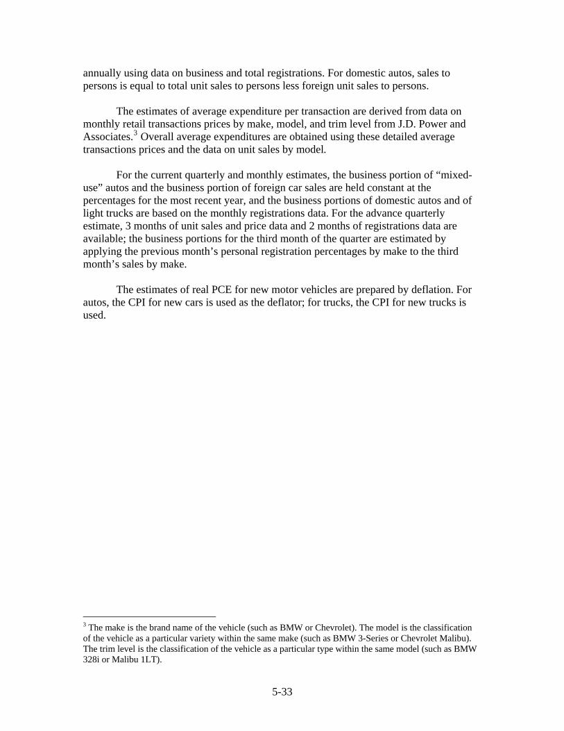
annually using data on business and total registrations. For domestic autos, sales to persons is equal to total unit sales to persons less foreign unit sales to persons.
The estimates of average expenditure per transaction are derived from data on
monthly retail transactions prices by make, model, and trim level from J.D. Power and Associates.3 Overall average expenditures are obtained using these detailed average transactions prices and the data on unit sales by model.
For the current quarterly and monthly estimates, the business portion of “mixed-
use” autos and the business portion of foreign car sales are held constant at the percentages for the most recent year, and the business portions of domestic autos and of light trucks are based on the monthly registrations data. For the advance quarterly estimate, 3 months of unit sales and price data and 2 months of registrations data are available; the business portions for the third month of the quarter are estimated by applying the previous month’s personal registration percentages by make to the third month’s sales by make.
The estimates of real PCE for new motor vehicles are prepared by deflation. For
autos, the CPI for new cars is used as the deflator; for trucks, the CPI for new trucks is used.
3 The make is the brand name of the vehicle (such as BMW or Chevrolet). The model is the classification of the vehicle as a particular variety within the same make (such as BMW 3-Series or Chevrolet Malibu). The trim level is the classification of the vehicle as a particular type within the same model (such as BMW 328i or Malibu 1LT).
5-33
Net purchases of used motor vehicles
In PCE, net purchases of used motor vehicles consists of dealers’ margins on purchases of these vehicles by persons and of net transactions between persons and other sectors of the economy. Net transactions for the personal sector are positive, because persons buy more vehicles from the other sectors than they sell to those sectors; in contrast, net transactions for business are negative.4 In calculating GDP, the intersectoral net transactions offset, leaving the margins on the transactions as value added. Separate estimates are made for used autos and for used light trucks.
Dealers’ margins
All purchases of used vehicles by persons from dealers include the retail
margin—the difference between the selling price and the dealer’s cost of acquisition. Additionally, they may include a wholesale margin (for vehicles sold to dealers by wholesalers) and sales taxes that are collected by dealers on behalf of government.
For benchmark years, total margins are estimated by applying margin rates and sales-tax rates to retail and wholesale sales of used motor vehicles. Then, the proportion of this total that applies to sales to persons is determined.5 Retail and wholesale margin rates are estimated using data from the Census Bureau’s Annual Retail Trade Survey (ARTS) and Annual Wholesale Trade Survey (AWTS). Wholesale and retail sales of used motor vehicles are based on product-line sales data from the Census Bureau’s Economic Census. Sales taxes are calculated using data from the Census Bureau’s Census of Governments, from individual states on tax collections, from ARTS, and from AWTS. For autos, almost all of the margin is allocated to sales to persons; for light trucks, the allocation to persons is based on information from the Census Bureau’s Vehicle Inventory and Use Survey.
For nonbenchmark years, total retail margins are estimated by applying margin
rates based on ARTS data to retail sales of used motor vehicles by new and used car dealers. Sales of used motor vehicles by new car dealers are valued based on unit sales and on an average selling price from the National Automobile Dealers Association (NADA); sales by used car dealers are derived as a percentage of their total sales from ARTS, based on product-line data from the economic census. The total retail margin is then allocated to used autos and to used light trucks based on data on changes in used vehicle unit registrations from R.L. Polk & Co. and on average prices of used vehicles sold at wholesale auctions from the Auto Dealers Exchange Service of America (ADESA). These auto and truck margins are then allocated to persons and to business based on ratios from the benchmark year. Finally, wholesale and retail taxes and
4 These values plus the associated margins are shown as “net purchases of used autos and used light trucks” in lines 9 and 18 in NIPA table 7.2.5B. 5 For a general discussion of the estimation of wholesale and retail margins and taxes, see U.S. Bureau of Economic Analysis, Concepts and Methods of the U.S. I-O Accounts, 8: 6–14, www.bea.gov/papers/pdf/IOmanual_092906.pdf.
5-34
wholesale margins on used vehicle sales are derived by extrapolation using changes in the retail margins.
The current quarterly and monthly estimates of margins on used autos and used
light trucks are extrapolated from the annual estimates, using R.L. Polk & Co. data on changes in used vehicle unit registrations and ADESA data on average auction prices.
The estimates of real margins are prepared by direct valuation (see the section
“Estimates for detailed components” in “Chapter 4: Estimating Methods”), using dealer unit sales times benchmark-year per-unit margins..
• Benchmark-year margins for sales of used motor vehicles by franchised new car dealers and by independent used car dealers are based on ARTS data on sales and cost of goods sold and on product-line sales data from the economic census. The nonbenchmark-year estimates are extrapolated using unit sales.
• Unit sales of franchised new car dealers are from NADA. Benchmark-year unit sales of independent used car dealers are derived by dividing product-line sales by average auction prices from ADESA. The nonbenchmark-year estimates are extrapolated using total sales of used car dealers from ARTS and the Census Bureau’s Monthly Retail Sales Survey divided by ADESA auction prices.
Estimates of total used vehicle margins of franchised new car dealers and of independent used car dealers are prepared and then summed to total used vehicle margins. This total is allocated between autos and light trucks, and between PCE and private fixed investment, using the same proportions as those derived for the current-dollar estimates. The real margin estimates are then scaled so that the current-dollar margins and the real margins are equal in the base year. The current quarterly estimates of real margins are extrapolated using R.L. Polk & Co. data on changes in used vehicle registrations. Net transactions
Net transactions between persons and other sectors of the economy primarily
consist of the wholesale value of purchases by persons from dealers less sales by persons to dealers (either directly or as trade-ins).6 In addition, transactions may occur between persons and businesses other than dealers (such as the sale of scrapped vehicles), government, and nonresidents. Transactions among persons are intrasectoral and so do not affect PCE.
For both benchmark and nonbenchmark years, estimates of net transactions are
developed by valuing the annual change in unit stocks of used motor vehicles held by persons, rather than by explicitly taking into account each type of transaction listed above. Yearend unit stocks of used autos and of used light trucks are estimated for each year of original sale (vehicles greater than 11 years old are grouped together) using annual data on new motor vehicle purchases and retention information developed from 6 For autos, net purchases also includes reimbursement of government employees for use of personal autos on government business.
5-35

R.L. Polk & Co. data on vehicles in use by model year.7 Unit stocks held by business are based on business purchases of new motor vehicles and on retention rates for rental vehicles (6–18 months), leased vehicles (2–4 years), and other business vehicles (1–9 years). Unit stocks held by government are based on government purchases of new vehicles and on assumed retention rates. Stocks held by persons are then calculated as the residual.
Changes in the unit stocks of autos and of light trucks held by persons reflect
purchases of new vehicles, scrappage of old vehicles, and net unit transactions other than scrappage. Purchases of new autos and of light trucks by persons are estimated separately (see the section “New motor vehicles”). Scrapped units are calculated by age of vehicle as a proportion of total vehicle scrappage; this proportion is assumed to be equal to the ratio of the unit stock held by persons to the total unit stock. Net unit transactions other than scrappage is then calculated as the residual.
The changes in unit stocks, grouped by age, are then valued at wholesale prices. The average wholesale value for each age group of used autos and of used light trucks is based on average auction prices by model year from ADESA. Scrapped units by age are valued at 8 percent of the wholesale price.
Current quarterly and monthly estimates of net transactions are extrapolated from
the annual estimates, using data on retail sales of used car dealers from the monthly retail trade survey. The estimates of real net transactions are prepared by deflation, using the CPI for used autos and trucks.
7 The year of original sale is the year in which the vehicle was sold as new. Thus, for example, the stock of used autos at yearend 2007 consists of all new autos that were sold in 2007, all new autos that were sold in 2006 and were not subsequently scrapped or otherwise disposed, and so on.
5-36
Motor vehicle fuels
The estimates of PCE for motor vehicle fuels are derived as the product of the quantity purchased for personal use and the average retail price per gallon. The estimates cover the personal use of motor fuel for all vehicles owned, leased, and rented by households. Quantities purchased
Except for the most recent year, separate annual estimates are made of the
quantities of motor fuel purchased for owned autos, for owned trucks, for leased vehicles, for rented vehicles, and for airplanes, motorcycles, and boats. For owned autos, purchases by persons are obtained as a residual after accounting for other uses. For motorcycles and boats, purchases by persons are estimated judgmentally as a portion of total purchases for these vehicles. For all other vehicles, purchases by persons are estimated directly.
For owned autos, the quantity of motor fuel purchased by persons for personal
use is calculated as follows: 1. The total quantity of motor fuel purchased for use in autos is equal to total
highway fuel purchases less purchases for buses, motorcycles, and trucks. Total highway fuel purchases are from the Federal Highway Administration’s (FHWA) Highway Statistics. Purchases of motor fuel for buses, none of which are for personal use, are also from the FHWA data. Purchases of motor fuel for motorcycles and for trucks are described below.
2. Fuel purchases for government-owned and business-owned autos are subtracted from total fuel purchases to derive fuel purchases for personal autos. For both business and government autos, fuel purchases are derived as the product of unit stocks and average fuel usage. Government unit stocks are from the FHWA, and business unit stocks are prepared by BEA (see “Net transactions” in the section “Net purchases of used motor vehicles”). Average fuel usage is calculated as average annual miles traveled divided by average miles per gallon (MPG). For government autos, average miles traveled is based on information from the U.S. General Services Administration’s (GSA) Motor Vehicle Fleet Report and from a Brookhaven National Laboratory survey of fleet operators. For business autos, average miles traveled is based on a survey of motor vehicle fleet operating expenses from the National Association of Fleet Administrators (NAFA), extrapolated by overall average annual miles traveled from FHWA data. MPG for government autos is based on GSA data, and MPG for business autos is based on NAFA data, extrapolated in each case by average model-year MPG for domestic autos from the U.S. Environmental Protection Agency.
3. Purchases by persons for personal use is equal to the total quantity of motor fuel purchased by persons for use in autos less the business portion of fuel purchased for “mixed-use autos”—that is, autos that are used for both business and personal transportation.
5-37
For owned trucks, the quantity of motor fuel purchased for personal use is
calculated as miles traveled divided by MPG. For benchmark years, total miles traveled for personal transportation is from the Census Bureau’s Vehicle Inventory and Use Survey (VIUS), and MPG is calculated as total miles traveled divided by total gallons used, based on personal transportation miles traveled by vehicles grouped by MPG range, also from VIUS. For nonbenchmark years, miles traveled is calculated as the product of stocks and average miles per vehicle; stocks (extrapolated from VIUS stock data), miles per vehicle, and MPG are estimated using corresponding FHWA data for all two-axle, four-tire trucks.
For leased and rented motor vehicles, which are part of the business stock, the
quantity of motor fuel purchased for personal use is estimated as follows. For leased vehicles, fuel purchases are calculated as miles traveled divided by MPG. Miles traveled is calculated as the product of unit stocks, which are based on personal lease registrations of new autos and new light trucks from R.L. Polk & Co. and on retention schedules based on the distribution of lease terms and of miles per vehicle, which is assumed by BEA to be 20 percent greater than the corresponding value for personally owned vehicles. MPG is assumed to be the same as that for all business autos. For rented vehicles, fuel purchases are estimated by assuming that the relationship of these purchases to total rental expenditures is the same as the relationship of fuel purchases for leased vehicles to total lease expenditures.
For other vehicles, quantities of fuel purchased for personal use are estimated
directly. Fuel purchased for airplanes is calculated as total gallons of gasoline consumed for aviation (which excludes jet fuel) from FHWA times a consumer share based on Federal Aviation Administration data on the proportion of hours flown in general aviation use that is accounted for by personal use. Total gasoline purchased for motorcycles is from the FHWA; BEA assumes that almost all is purchased by persons. Total gasoline purchased for boats is also from the FHWA; BEA assumes that two-thirds is purchased by persons.
Average retail price
The average retail price per gallon is calculated as total expenditures divided by
total gallons. Expenditures are estimated for each grade of gasoline as the product of gallons sold, based on gallons supplied to retailers by grade from the Energy Information Administration’s (EIA) Petroleum Marketing Annual, and on an average retail price by grade, based on monthly prices from BLS. The expenditures by grade are then summed to total expenditures and divided by total gallons supplied. Most-recent-year and current-quarterly estimates
The most-recent-year and the third quarterly estimates of PCE for gasoline and
other motor fuel are prepared by extrapolating from the preceding annual estimate using total expenditures for gasoline, based on quantities from EIA and prices from BLS, by
5-38
grade. For the second quarterly estimate, EIA data on monthly quantities by grade are available for the first 2 months of the quarter, and EIA data for total gasoline supplied are used for the third month. For the advance quarterly estimate, monthly quantities by grade are available for the first month, monthly total gasoline supplied is available for the second month, and weekly EIA data on total gasoline supplied are used for the third month. For the months for which quantities by grade are not available, the estimate is based on the total gasoline supplied times the CPI for motor fuel.
Quantity estimates
The estimates of real PCE for motor vehicle fuel are prepared by deflation using the CPI for motor fuel.
5-39

Rental of tenant- and owner-occupied nonfarm housing
As noted in “Chapter 2: Fundamental Concepts,” purchases of newly constructed housing are treated as private fixed investment rather than as consumption expenditures in the NIPAs, and the stock of housing is treated as fixed assets. The housing stock provides a flow of housing services that are consumed by persons who rent their housing and by persons who own the housing they occupy (referred to as “owner-occupants”). In the NIPAs, owner-occupants are treated as owning unincorporated enterprises that provide housing services to themselves in the form of the rental value of their dwellings.8 Thus, PCE for housing services includes both the monetary rents paid by tenants and an imputed rental value for owner-occupied dwellings (measured as the income the homeowner could have received if the house had been rented to a tenant). This treatment is designed to make PCE (and GDP) invariant to whether the house is rented by a landlord to a tenant or is lived in by the homeowner.9 PCE for rental of tenant-occupied dwellings is based on the rent paid by tenants—which may include charges for major appliances and furnishings, utilities, or services. The rent paid is then adjusted to exclude any utility payments and to include tenant expenditures for major replacements, maintenance, and repairs that are not reimbursed by the landlord owner. Payments for utilities are subtracted because they are already accounted for elsewhere in PCE, and tenants’ unreimbursed expenditures are added because they are considered part of the rental cost to the tenant. The rental value of owner-occupied dwellings is based on that of equivalent tenant-occupied dwellings, but it consists of the rental value of the dwelling alone.
Separate estimates are prepared for owner-occupied permanent-site dwellings, owner-occupied mobile homes, tenant-occupied permanent-site dwellings, and tenant-occupied mobile homes. For each type of dwelling, rent equals the number of occupied units times the rent per unit. Number of housing units
The benchmark estimates of units for each type of dwelling are based on data
from the Census Bureau’s decennial Census of Housing (COH).10 For tenant- and owner-occupied permanent-site homes, the number of units from the COH is adjusted by BEA to reflect the stock at midyear and to account for certain vacant units, such as vacation homes.
8 This treatment is consistent with that of the international System of International Accounts (SNA): “Households that own the dwellings they occupy are formally treated as owners of unincorporated enterprises that produce housing services consumed by those same households” (SNA 2008: 6.117). 9 According to the SNA, “The ratio of owner-occupied to rented dwellings can vary significantly…so both international and inter-temporal comparisons of the production and consumption of housing services could be distorted if no imputation were made for the value of own-account housing services.” (SNA 2008: 6.34). 10 Thus, in the comprehensive revision of the NIPAs, the benchmark estimates for PCE for housing services are made for the years ending in “0,” and the estimates for other years are nonbenchmark annual estimates.
5-40
For permanent-site (or stationary) homes, nonbenchmark annual estimates are interpolated and extrapolated from the benchmark estimates. For years for which data from the Census Bureau’s biennial American Housing Survey (AHS) are available, unit stocks from the AHS are used as the indicator series; for other years, data from the Census Bureau’s Current Population Survey are used to interpolate and extrapolate the AHS-based estimates. For mobile (or manufactured) homes, the indicator series is based on changes in unit stocks that are derived from data on shipments of manufactured homes in the Census Bureau’s Monthly Construction Statistics, using a perpetual inventory calculation (see “Chapter 4: Estimating Methods”). Rent per unit
For tenant-occupied permanent-site dwellings, the benchmark estimates of rent
per unit are based on COH data on units by rent class. The charges for utilities—energy (electricity, gas, and fuel oil and other fuels) and water and sewerage maintenance—that must be subtracted from rent are estimated as follows:
• The PCE estimates for each type of energy are allocated between tenant-occupied housing and owner-occupied housing using data from the Department of Energy’s Residential Energy Consumption Survey (RECS), and the portion of the tenant expenditures for energy that is included in rent is derived using AHS data. In the cases where the RECS or AHS are not conducted in the benchmark year, proportions derived from surveys in nearby years are interpolated for the benchmark estimates.
• PCE for water and sewerage maintenance is allocated between tenant-occupied housing and owner-occupied based on the tenant-occupied share of total nonfarm permanent-site units, and the portion of the tenant expenditures that is included in rent is derived using AHS data. The nonbenchmark annual estimates of rent per unit less utilities are derived from
data on average rental value that includes expenditures for utilities whether they are paid separately or included in rent, so these data must be adjusted to exclude average utility payments. The average rental value is benchmarked using COH data on units by rent class and is interpolated and extrapolated using AHS data on units by rent class. In non-AHS years, this rental value is interpolated and extrapolated from the AHS estimates using the CPI for rent of primary residence. Average expenditures for utilities are calculated as total expenditures for utilities (estimated as described above) divided by total tenant-occupied units.
The rental value of appliances and furnishings provided by property owners is
equal to BEA’s estimate of depreciation at current replacement cost. For both benchmark and nonbenchmark years, tenants’ unreimbursed expenditures for major replacements and for maintenance and repairs—originally reported in the Census Bureau’s Survey of Residential Alterations and Repairs—are extrapolated using data from the BLS Consumer Expenditure Survey (CEX).
5-41
For owner-occupied permanent-site homes, the benchmark estimates of rent per unit are derived using landlord-reported rent receipts and housing values from the Census Bureau’s Residential Finance Survey, which is conducted in conjunction with the COH.11
1. A unit-weighted average rent-to-value ratio is estimated for each market-value class of one-unit tenant-occupied dwellings.
2. This ratio is multiplied by a midpoint housing value for the class to derive an average rent per unit for each value class.
3. The average rent per unit for each value class is multiplied by the corresponding number of owner-occupied units to derive imputed rent receipts for these units.
4. Rent receipts and owner-occupied units are summed across all value classes and then the former is divided by the latter to derive an imputed average rent for owner-occupied permanent-site homes. The nonbenchmark annual estimates of owner-occupied contract rent per unit are
prepared by extrapolation using the product of (1) the CPI for owners’ equivalent rent, which captures changes in the rental value of constant-quality owner-occupied dwellings, and (2) the constant-dollar per-unit value of owner-occupied nonfarm dwellings, which captures changes in the rental value that result from changes in the average quality of these dwellings. The constant-dollar per-unit values are derived by dividing the BEA estimates of constant-dollar net stocks by the corresponding unit stock.
For all years, the rental value of the dwelling alone (or “space rent”) for owner-
occupied permanent-site homes is derived by multiplying the rent excluding utilities by the number of owner-occupied units and then subtracting BEA’s estimate of current-cost depreciation of major appliances.
For tenant-occupied manufactured homes, the estimates of rent per unit are derived as rent (which may include utilities) plus separately paid utilities less average utility payments. Benchmark estimates of average rent per unit are based on rental-value-range and unit data from the COH. For owner-occupied manufactured homes, gross rent per unit is estimated as the product of rent per unit of tenant-occupied units and the ratio of the average number of rooms in owner-occupied units to those in tenant-occupied units. For nonbenchmark years, average rent is interpolated and extrapolated using median rent from AHS, or for non-AHS years, using the CPI for rent of primary residence. Data on average utility payments are from RECS, interpolated and extrapolated using the product of the number of units and of the CPI for gas (piped) and electricity. Current quarterly and monthly estimates
The quarterly and monthly current-dollar estimates are prepared by reflating the
estimates of real PCE for each type of dwelling using the CPI for rent of primary residence for tenant-occupied dwellings and the CPI for owners’ equivalent rent of
11 According to the SNA, “When well-organized markets for rented housing exist, the output of own-account housing services can be valued using the prices of the same kind of services sold on the market…” (SNA 2008: 6.117).
5-42
primary residence for owner-occupied dwellings. The monthly estimates in real terms are based on the number of units for each type of dwelling adjusted for changes in the quality of the housing stock. Stocks of permanent-site homes are interpolated and extrapolated from the annual estimates, using monthly Census Bureau data on housing completions. The total stock of manufactured homes is estimated by interpolating and extrapolating from the annual estimates, using monthly Census Bureau data on shipments of manufactured homes (for the advance quarterly estimate, the shipments data are available only for the first 2 months of the quarter). The distributions of the permanent-site stock and of the manufactured home stock between owner-and tenant-occupied units are based on recent trends. The unit estimates are adjusted for changes in the quality of the housing stock based on historical relationships between average rental values and the respective CPIs. Quantity estimates
The estimates of the real rental value of tenant-occupied nonfarm dwellings are
derived by deflation: the CPI for rent of primary residence is used to deflate space rent, and the CPI for major appliances is used to deflate depreciation at current-replacement costs of major appliances and furnishings provided by property owners. The estimates of the real rental value of owner-occupied nonfarm dwellings are derived by deflation using the CPI for owners’ equivalent rent of primary residence.
5-43
Financial service charges and fees
This PCE services component consists of commercial bank service charges on deposit accounts, commercial bank and nondepository credit intermediation fees on credit card accounts, and other financial service charges and fees. Commercial bank service charges on deposit accounts
Benchmark estimates are based on Census Bureau’s Economic Census data on
fees for individual deposit account services (other than ATM and electronic transactions fees) and fees for bundled deposit account services. Nonbenchmark annual estimates are interpolated and extrapolated using data on total service charges on deposit accounts of commercial banks from Statistics on Depository Institutions produced by the Federal Deposit Insurance Corporation (FDIC). For the current quarterly estimates, the third estimate is also based on the FDIC data, and the second and advance estimates are judgmentally trended. Commercial bank and nondepository credit intermediation fees on credit card accounts
. Fees on credit card accounts consist of membership fees, cash advance fees, late
fees, over-limit fees, and other miscellaneous credit card fees.12 The benchmark estimates are equal to cardholder fees reported in the economic census times a consumer share based on the noncommercial share of bank card purchases from the Nilson Report, a credit-card industry newsletter. Nonbenchmark annual estimates of credit card fees are interpolated and extrapolated using data on bank card dollar-volume data from CardWeb.com Inc. The third quarterly estimate is extrapolated using CardWeb.com Inc. data, and the advance and second estimates are judgmentally trended.
Other financial service charges and fees
This category consists of commercial bank other fee income, savings institution
and credit union charges and fees, activities related to credit intermediation charges and fees, and postal money order and money transfer services fees.
Commercial bank other fee income consists of automated teller machine (ATM)
and other electronic transactions fees, consumer loan fees, and other fees. Benchmark estimates of ATM and other electronic transactions fees are based on fees for individual deposit accounts reported in the 2002 Economic Census. Benchmark estimates of fees on unsecured consumer loans are also based on economic census data. Other fees are based on data on safe deposit box rental charges reported in the BLS Consumer Expenditure Survey. Nonbenchmark annual estimates are interpolated and extrapolated using FDIC data on “additional noninterest income.”
12 Service charges and fees on credit card accounts do not include finance charges, which are included in personal interest payments.
5-44
Savings institution and credit union charges and fees consists of service charges on deposit accounts, service charges and fees on credit card accounts, ATM and other electronic transaction fees, and fees on unsecured consumer loans. The benchmark estimates are based on economic census data. Service charges on deposit accounts and ATM and other electronic transactions fees equal fees for individual deposit accounts, and consumer loan fees are based on fees for unsecured consumer loans. Service charges and fees on credit card accounts equal cardholder fees times a consumer share based on the non-commercial share of bank card purchases from the Nilson Report.
The nonbenchmark annual estimates of PCE for savings institutions are
interpolated and extrapolated using the sum of Office of Thrift Supervision (OTS) data on nonmortgage fees and charges for OTS-regulated savings institutions and of FDIC data on service charges on deposit accounts and income from fiduciary accounts of FDIC-regulated savings institutions. For credit unions, the nonbenchmark annual estimates are interpolated and extrapolated using data on fee income and other operating income from the National Credit Union Administration.
Activities related to credit intermediation charges and fees consists of ATM and
other electronic transaction fees, automated clearing house (ACH) and other electronic transaction fees, credit card charges and fees, and check cashing and other payment product fees. The benchmark estimates are based on economic census data, including payment product fees of commercial banks and other depository institutions. The nonbenchmark annual estimates are interpolated and extrapolated using BLS Quarterly Census of Employment and Wages data on other activities related to credit intermediation wages and salaries.
For postal money order fees, benchmark and nonbenchmark annual estimates are
based on money order fees reported by the U.S. Postal Service, adjusted from a fiscal year basis to a calendar year basis.
For money transfer services fees, benchmark and nonbenchmark annual estimates
are based on payment services revenue data from Form 10K annual reports filed by First Data Corporation and Moneygram International with the Securities and Exchange Commission. Revenue data are adjusted to total money transfers and then to transfers originating in the United States based on information from the company reports, and these revenues are then allocated almost entirely to consumers.
The current quarterly estimates of other financial service charges and fees of other
depository institutions are judgmentally trended. The quantity estimates for all components of PCE for financial service charges
and fees are prepared by deflation, using the CPI for checking account and other bank services.
5-45

Securities commissions
This PCE services component consists of direct commissions on securities transactions, of indirect commissions on securities transactions, and of mutual fund sales charges.
Direct commissions
Direct commissions—those for which an explicit commission is charged—consist
of commissions on equities transactions executed on an exchange and of commissions on all other securities transactions, including equities transactions executed on over-the-counter (OTC) markets and transactions in debt securities.13
The benchmark estimates of total commissions on equities and on debt securities
are based on data from the Census Bureau’s Economic Census. Total equities commissions are allocated between exchange-traded equities and equities traded on OTC markets using commissions data by market from Securities and Exchange Commission (SEC) tabulations of Financial and Operational Combined Uniform Single (FOCUS) Reports filed by broker-dealers. Then, commissions charged to other brokers from FOCUS Report data are subtracted to derive commissions charged to the public.
Equities commissions charged to the public are allocated to persons using
estimates of shares traded by individuals and institutions and of cents-per-share commission rates. Estimates of shares traded, which reflect the purchasing and selling sides of share volume, are derived as follows.
1. For registered exchanges, shares traded by the public equal total shares traded less member trading.
a. For the New York Stock Exchange (NYSE), share volume and member purchases and sales are reported by the exchange.
b. For other registered exchanges, share volume is reported by the SEC, and member purchases and sales are estimated by applying the American Stock Exchange member percentage to total purchases and sales.
2. For OTC markets, shares traded by the public equal public-to-public trading and the public side of dealer-to-public transactions.
a. Public-to-public share volume is based on National Association of Securities Dealers Automated Quotation (NASDAQ) data on electronic communication networks.
b. Dealer-to-public trading volume is derived from total trading volume and estimates of public-to-public and dealer-to-dealer volume. Total OTC volume is reported by NASDAQ, and dealer-to-dealer volume is based on National Association of Securities Dealers estimates of the share of total volume accounted for by these transactions.
13 Debt securities consist of negotiable certificates of deposit, commercial paper, bankers acceptances, U.S. Treasury bills, other money market instruments, corporate and trust notes and bonds, U.S. government notes and bonds, and state and local government notes and bonds.
5-46
3. The shares of public trading accounted for by individuals on the NYSE, on other registered exchanges, and on OTC markets were each initially based on Securities Industry Association (SIA) reports and are now extrapolated by the household shares of corporate equity holdings based on Federal Reserve Board’s Flow of Funds data.
The estimates of cents-per-share commission rates on registered exchanges and on OTC markets are based on total commissions, the institutional and individual percentages of public-share volume, and the assumption that individual commission rates are twice the institutional rates, based on an SEC survey of commission rates.
To the equities commissions charged to individuals are added commissions
charged to nonprofit institutions serving households (NPISHs). First, the share of total commissions charged to all nonprofit institutions is estimated using flow of funds data on corporate equity holdings. Then, the NPISH share of the nonprofit commissions is estimated using IRS data on the NPISH share of securities investments of tax-exempt organizations. The allocation of NPISH commissions between registered exchanges and OTC markets is the same as that for individual commissions.
The benchmark estimates of commissions on debt transactions are derived as the
product of total commissions charged to domestic purchasers and of a consumer share based on the percentage of marketable debt securities held by households from flow of funds data.
For nonbenchmark years, equities commissions on registered exchanges are
extrapolated using FOCUS Report data on total commissions on equity transactions executed on exchanges less commissions charged to other brokers. The allocation of commissions charged to individuals and to NPISHs is based on shares traded by individuals and institutions on registered exchanges and on an assumed ratio of individual to institutional commission rates. Other direct commissions, which consist of commissions on OTC equities transactions and on debt transactions, are extrapolated using FOCUS report data on OTC commissions less commissions charged to other brokers. The allocation to individuals is based on shares traded by individuals and institutions on OTC markets and on the assumed ratio of individual to institutional commission rates.
For the current quarterly estimates, FOCUS Report commissions data are used to
extrapolate the third estimate, and NYSE round lot and odd-lot share volume and NASDAQ OTC share volume are used to extrapolate the second and advance estimates.
The estimates of real direct commissions on exchange-listed equities are prepared
by deflation, using the “PPI for brokerage services, exchange-listed equities.” Direct commissions on OTC equities and on debt transactions are deflated using the “PPI for brokerage services, all other securities.”
5-47
Indirect commissions Indirect commissions—those for which the commission is charged indirectly
through a dealer markup or “spread”14—comprise commissions on OTC equity securities and other indirect commissions, which consist of gains from specialist transactions in equities on registered exchanges and from brokering and dealing debt securities and derivatives.15
The benchmark estimates of total indirect commissions on equities, debt
securities, and derivatives are based on data from the economic census on net gains (excluding interest income) in trading accounts for brokering and dealing securities. For equities, the allocation of total indirect commissions to persons is made using the personal share of equities holdings (including NPISHs and bank personal trusts and estates). The personal share of equities holdings is based on averages of yearend holdings from flow of funds data. Total PCE for indirect commissions on equities transactions is allocated between OTC markets and registered exchanges using estimates based on total shares sold and cents-per-share spreads.
• For OTC markets, individual purchases from dealers are equal to total dealer sales to the public less purchases by institutions. Total dealer sales to the public is derived by subtracting dealer-to-dealer and public-to-public share volume from the total and using a BEA assumption that one-half of the remaining dealer-to-public transactions is accounted for by sales. The institutional share of OTC transactions is based on SIA reports. Average cents-per-share spreads are from NASDAQ, extrapolated by the “PPI for dealer transactions, market making in over-the-counter equities.”
• For registered exchanges, the NYSE ratio of specialist sales to total purchases and sales is applied to total purchases and sales on all registered exchanges to derive total specialist sales. The individual share of specialist sales is based on SIA reports. Average cents-per-share spreads are assumed to equal the volume-weighted spread for NYSE specialists as reported by the exchange.
To indirect commissions charged to individuals are added commissions charged
to NPISHs, based on the nonprofit share of total corporate equity holdings from flow of funds data applied to total indirect commissions and an allocation of nonprofit commissions to NPISHs based on IRS data.
The benchmark estimates of indirect commissions on transactions in U.S.
government and agency securities, in municipal securities, and in corporate debt securities are allocated to persons using the personal share of holdings (including NPISHs and bank personal trusts and estates). The personal share of equities holdings is based on averages of yearend holdings from flow of funds data. The allocation of benchmark
14 Dealers who make markets in securities do not charge commissions; instead, they retain as compensation the income resulting from acquiring securities at a price lower than the price at which the securities are subsequently sold to their customers. 15 Derivatives consist of futures contracts, option contracts, forward contracts, swaps, and other derivative contracts.
5-48
estimates of commissions on derivatives to persons is based on an assumed 15-percent share.
For nonbenchmark years, PCE for indirect commissions on OTC equities is
extrapolated by the product of OTC share volume (excluding matched volume) from NASDAQ and of the “PPI for dealer transactions, market making in over-the-counter equities.” PCE for other indirect commissions is estimated in three parts: specialists’ gains on equities trading on registered exchanges, gains on brokering and dealing debt securities, and gains on brokering and dealing derivatives.
• Specialists’ gains are extrapolated by specialists’ sales from the NYSE. • Gains on debt securities are estimated for U.S. government securities, for
U.S. government agency and government-sponsored enterprises securities, for state and local government debt securities, for corporate debt securities, and for open-market paper. In each case, total indirect commissions are extrapolated by the value of trading and allocated to persons (including NPISHs) based on the share of each type of security held by persons, based on flow of funds data. The source for U.S. government and for agency securities is total primary dealer sales excluding other brokers and dealers, from Federal Reserve Bank of New York (FRBNY) data. For state and local government securities and for corporate debt securities, the value of trading is from the Securities Industry and Financial Markets Association (SIFMA). For open-market paper, the source is primary dealer volume with others in corporate debt securities due in less than 1 year, from FRBNY data.
• Derivatives commissions are extrapolated in two parts: options and future and forward contracts. Options commissions are extrapolated using SEC data on the value of options trading. Commissions on futures and forward contracts are extrapolated using futures contracts data from the Futures Industry Association.
The current quarterly estimates of indirect commissions of OTC equities
transactions are extrapolated using the value of OTC trading from NASDAQ. Other indirect commissions are extrapolated using FRBNY data on dealer transactions with others in U.S. government, federal agency, and government-sponsored enterprise securities.
The estimates of real OTC equities commissions are prepared by deflation, using
the “PPI for dealer transactions, market-making in over-the-counter equities.” For other indirect commissions, the “PPI for dealer transactions, debt securities, and all other trading” is used as the deflator. Broker charges on mutual fund sales . The benchmark estimates of total broker charges on mutual fund sales are based on economic census data. Charges for nonbenchmark years are interpolated and extrapolated using data on revenue from the sale of investment company securities from
5-49

the FOCUS Report. Commissions are allocated to individuals, fiduciaries, and nonprofits based on data on their respective shares of mutual fund assets from the Investment Company Institute (ICI). For current quarterly estimates, the third estimate is extrapolated using data on charges on the sale of investment company securities from the FOCUS Report, and the second and advance estimates are extrapolated using data on sales of mutual fund shares reported by the ICI. The estimates of real broker charges on mutual fund sales are derived by quantity extrapolation, using an indicator equal to mutual fund sales from the ICI deflated by the all-items CPI.16
16 For a general description of the quantity extrapolation method, see “Chapter 4: Estimates for Detailed Components.”
5-50
Financial services furnished without payment
This PCE services component includes depository institutions—commercial banks, savings institutions, and credit unions—and regulated investment companies (mutual funds), which provide services to persons without explicitly charging for these services.17 This component also includes pension plans—private noninsured pension plans and publicly administered government employee retirement plans—which earn property income (dividend, interest, and rental income) on plan reserves that have been contributed directly by, or are held for the benefit of, beneficiaries and that will be paid out to them as annuity or lump-sum distributions of income in the future. In the NIPAs, the value of both of these types of services is imputed to PCE as financial services furnished without payment in order to make PCE invariant to whether the charges are implicit or explicit.
In the NIPAs, imputations are made for the value of the services (such as check
clearing, recordkeeping, and investment services) that are provided by depository institutions.18 For commercial banks, services to borrowers are estimated as the difference between the rate of return on loans and a riskless “reference rate”—measured as the average rate earned by banks on U.S. government and agency securities—times the value of the loans.19 Services to depositors are estimated as the difference between the reference rate and the rate paid on deposits times the value of deposits. These estimates are based on the premise that rather than pay explicit fees, borrowers accept a higher interest rate, and depositors a lower rate, than they would otherwise. The differences in interest rates are used to infer the implicit value of the services that the banks are providing to their customers. Interest flows are adjusted because a portion of the money paid as interest by borrowers represents a payment for these services and because the interest forgone by depositors reflects the value of the services they receive.
The implicit services provided by other depository institutions—savings
institutions and credit unions—are allocated entirely to depositors. They are calculated as the difference between interest earned on loans and interest paid on deposits. Imputations are also made for the value of the services that are provided by regulated investment companies (RICs) to their shareholders. These imputed service charges are equal to the operating expenses of the RICs.
The imputations for these services are recorded in the Personal Income and
Outlay Account of the summary NIPAs as follows.20 Personal interest income (and personal income) is raised by an amount equal to the imputed service charges for the
17 The value of these services to government is imputed to government consumption expenditures and that to foreigners is imputed to exports of services. For business, these services are considered intermediate consumption and cancel out in the consolidation of the production account of the business sector. 18 See Brent R. Moulton and Eugene P. Seskin, “Preview of the 2003 Comprehensive Revision of the National Income and Product Accounts,” Survey 83 (June 2003): 23–27; see also Dennis J. Fixler, Marshall B. Reinsdorf, and George M. Smith, “Measuring the Services of Commercial Banks: Changes in Concepts and Methods,” Survey 83 (September 2003): 33–44. 19 The calculation of the reference rate excludes mortgage-backed securities. 20 For a discussion of the summary NIPAs, see “Chapter 2: Fundamental Concepts.”
5-51
depositor and investor services. In personal outlays, PCE is raised by the sum of the imputed service charges for depositor and investor services and for borrower services, and personal interest payments is reduced by the imputed service charges for borrower services, since a portion of the interest payment is assumed to represent a fee for unpriced borrower services. Thus, personal outlays is raised by the same amount as personal interest income, and personal savings is not affected by the imputations.
In the NIPAs, pension plans are regarded as charging participants an implicit fee that is equal to the plans’ administrative expenses for the package of imputed services provided. The property income of pension plans is recorded in personal income as monetary interest, dividends, and rental income as appropriate, and the difference between this income and the imputed fees is recorded as personal saving. The benefit payments associated with pension plans are treated as transfers within the personal sector; such intrasectoral transactions are not recorded in the NIPAs. In effect, the NIPA treatment performs a timing change so that the property income that has been accrued to the plan beneficiaries is recorded as if it were actually disbursed to them in the current period.
Commercial banks
The value of implicit commercial bank services to depositors is based on average
deposit balances and on a “user-cost price” that is calculated as the difference between the reference rate and the interest rate paid on deposits. Similarly, the value of commercial bank services to borrowers is based on average loan balances and on a user-cost price that is calculated as the difference between the interest rate earned on loans and the reference rate. The estimates of deposits and of loan balances, of interest paid and received on deposits and loans, and of the reference rate are all based on data from the Federal Financial Institutions Examination Council’s (FFIEC) Call Reports.
For each type of deposit and for loans21 in domestic offices of U.S. chartered banks, an average rate of interest is derived from the average balance and interest income or expense, and the user-cost price is calculated as the difference between the average interest rate and the reference rate. The value of the implicit service is calculated by applying the user-cost price to the average deposit or loan balance, with an adjustment to include balances in U.S. offices of foreign banks. Imputed services to depositors are equal to the sum of services to all types of deposit accounts—demand deposit accounts (noninterest-bearing checkable deposits) and interest-bearing accounts (checkable deposit accounts, savings accounts, and time deposit accounts)—except intrabank deposits.
The share of total imputed demand-deposit services that is allocated to persons is
based on the share of demand deposits held by persons. This share was initially based on a since-discontinued Federal Reserve Board (FRB) survey of demand deposit ownership. The personal share of demand deposits is no longer available, so the original estimate from the FRB survey is extrapolated using the household share of transactions deposits (which include interest-bearing checkable deposits as well as demand deposits) as 21 Also includes capital leases.
5-52
follows. FFIEC data on total transactions deposits in domestic offices are adjusted to exclude deposits held by commercial banks and other depository institutions, and deposits held by individuals, partnerships, and corporations are calculated as a percentage of the adjusted total. FRB Flow of Funds data on the distribution of checkable accounts among households and types of business are then used to determine the household share of the adjusted transactions deposits.
For interest-bearing deposits, there are no data on the share of these deposits held
by persons, so the allocation of implicit services to persons is based on the household share of interest-bearing deposits excluding checkable deposits (which include money market deposit accounts, other savings deposits, and time deposits) derived from FFIEC and flow of funds data. The FFIEC total of these deposits is adjusted to exclude holdings of foreign governments and official institutions, and the percentage of deposits held by individuals, partnerships, and corporations is calculated. Flow of funds data on the distribution of savings and time deposits among households and types of businesses are then used to determine the household share of the adjusted deposits total.
The imputed borrower services are allocated to persons based on FFIEC data on
the share of outstanding loans that is accounted for by credit card and other consumer loans.
Annual quantity estimates. The annual estimates of real PCE for commercial bank
services are derived using a BLS banking output index that is based on volume measures for the deposit, loan, and trust functions of commercial banks. There are component indexes for U.S.-owned banks and for U.S. offices of foreign banks, each of which use employment weights that are based on data from the Federal Reserve banks’ Functional Cost Analysis Report.
• For U.S.-owned banks, the BLS deposit index consists of a demand deposit component, based on the number of checks processed and the number of electronic transactions; a time deposit component, based on estimated deposits and withdrawals; and an ATM component, based on ATM and point-of-sale volume. The BLS loan index is based on the number of real estate, consumer, and commercial loans outstanding and on the volume of credit card transactions.
• For U.S. offices of foreign banks, the indexes for deposits and for loans are based on the number of deposit accounts and loans, which are estimated from the total value loans reported in the FRB Share Data for the U.S. Offices of Foreign Banking Organizations report and on average deposit and loan sizes.
The U.S.-owned and foreign-owned banking output indexes are combined using revenue data from the Census Bureau’s Economic Census that are extrapolated by assets and aggregated using a Tornqvist aggregation procedure.
The BLS banking output index is used to extrapolate the total value of priced and
unpriced banking services from the base-year value. From the extrapolated value, the real-dollar value of explicit service charges and fees (see the section “Financial service
5-53
charges and fees”) is subtracted to obtain the real-dollar value of unpriced banking services, which is then allocated to persons in the same proportion as the current-dollar estimates. For the most recent year, the BLS banking output index is extrapolated using available data on deposit, loan, and trust activity.
Current quarterly estimates. For the current-dollar estimates, the third quarterly
estimate for commercial bank services is derived by extrapolation, using FFIEC data on deposit and loan values, on interest paid and received, and on the reference rate. The second and advance estimates are judgmentally trended. The current quarterly estimates of real commercial bank services are judgmentally trended. Other depository institutions
The value of implicit services to depositors is estimated for mutual savings banks,
for savings and loan institutions, and for credit unions. For these institutions, implicit services equal the sum of monetary interest received on loans and of other property income less monetary interest paid on deposits and less profits before tax (for savings and loans, only the profits of mutual institutions are deducted). Estimates for all years are derived from data on interest paid and received from the Federal Deposit Insurance Corporation, the Office of Thrift Supervision, and the Credit Union National Association. For mutual savings banks and for savings and loans, profits of mutual institutions are from IRS tabulations of corporate income tax returns; for credit unions, they are from tabulations of net interest less dividends to shareholders and interest refunds by the National Credit Union Administration. For savings and loans, the consumer share is based on the value of deposits of $100,000 or less as a percentage of total deposits from FRB tabulations of Thrift Financial Report data. For mutual savings banks and for credit unions, all imputed service charges are allocated to persons.
Annual quantity estimates. The annual estimates of the real implicit services
provided by other depository institutions are derived by deflation, using the PCE implicit price deflator for services furnished without payment by commercial banks.
Current quarterly estimates. The current-dollar quarterly estimates of the implicit
services provided by other depository institutions are judgmentally trended. The current quarterly estimates in real terms are also judgmentally trended. Regulated investment companies
The total value of imputed services of RICs equals their operating expenses.
These expenses are measured as “total deductions” from IRS income statement data on open-end investment funds, plus securities commissions and “services furnished without payment” by other financial intermediaries. Securities commissions include direct commissions paid on equities and options transactions and indirect commissions paid on equities, debt securities, and options transactions. For the most recent year, “total deductions” are extrapolated using data on mutual fund total net assets from the Investment Company Institute (ICI).
5-54
For all years, direct commissions paid by RICs are estimated as a share of total
institutional commissions paid by U.S. residents. The methodology used to derive the estimates of total direct commissions charged to the public and of individual and institutional commissions is described in the section “Securities commissions.” Commissions paid by foreign residents, which are included in institutional commissions, are estimated by applying the foreign share of the value of total purchases and sales of U.S. equities to total commissions charged to the public. The value of foreign residents’ transactions in U.S. equities is from BEA’s International Transactions Accounts data; the value of total purchases and sales is from the New York Stock Exchange, the National Association of Securities Dealers Automated Quotation System for over-the-counter markets, and the Securities and Exchange Commission for other registered exchanges. The RIC share of institutional commissions paid by U.S. residents is equal to equity holdings of mutual funds as a percentage of total equity holdings of domestic institutions, based on flow of funds data.
The share of total indirect commissions that is accounted for by RICs is estimated
separately for equities, U.S. treasury securities, U.S. government agency and government-sponsored enterprise securities, municipal securities, corporate debt securities, and options transactions. The derivation of total indirect commissions for all types of securities is described in “Securities commissions.” For each type of security except options, the allocation to RICs is based on the RIC share of total marketable securities averaged from yearend flow of funds data. The allocation of indirect commissions on options transactions assumes the same distribution as that for the total on debt and equity securities net transactions.
The allocation to persons of RIC services is based on flow of funds data on the
share of mutual fund assets that are held by the household sector. “Services furnished without payment” by other financial intermediaries comprise
the implicit depositor services of depository institutions. These services are allocated to RICs in proportion to the RIC shares of deposits, which are derived by the same method as described above for commercial banks and other depository institutions.
Annual quantity estimates. The annual estimates of real implicit RIC services are
derived by deflation. For direct and indirect commissions, several PPIs for brokerage services are used as deflators. For all other expenses, a BEA input cost index—based on several PPI components and on the BLS Employment Cost Index (ECI) for the finance, insurance, and real estate sector—is used as the deflator.
Current quarterly estimates. The current-dollar quarterly estimates of implicit
RIC services are extrapolated using a 3-month moving average of mutual fund total net assets from the ICI. The estimates in real terms are prepared by deflation, using a BEA input cost index that is based on several PPI components and on the quarterly ECI for finance, insurance, and real estate. The ECI data is available for the third quarterly
5-55
estimate, and it is interpolated and extrapolated by average hourly earnings for portfolio management from BLS’ Current Employment Statistics (CES).
Pension plans
For private noninsured pension plans, the annual estimates of PCE are calculated
as the sum of reported expenses of employee benefit plans and of securities commissions paid by these plans. Reported expenses are based on BEA tabulations of annual report data (Form 5500) from the Department of Labor’s Employee Benefits Security Administration. Reported expenses are not available for the most recent 2 years, so the estimates for those years are judgmentally trended. Securities commissions include both direct and indirect commissions on equity and debt securities and on options and are estimated as described in “Securities commissions.” These commissions are allocated to pension plans using flow of funds data on the distribution of securities holdings.
For publicly administered government employee retirement plans, the annual
estimates of PCE are calculated as the sum of the administrative expenses of the federal government plans and the administrative expenses and indirect securities commissions of the state and local government plans. The estimates of the administrative expenses for the federal plans—which consist of federal civilian and military retirement funds, the Thrift Savings Plan, and the Uniformed Services Retiree Health Care Fund—are based primarily on data from the U.S. Department of Treasury’s Monthly Treasury Statement. The estimates of the administrative expenses for the state and local government employee retirement plans are based on retirement systems data from the Census Bureau’s annual Survey of Government Finances. The estimates of indirect commissions on securities transactions are described in “Securities commissions” and are allocated to state and local government pension funds using flow of funds data.
For the most-recent-year, the expenses of pension plans are extrapolated using
BLS Quarterly Census of Employment and Wages (QCEW) data on pension fund industry wages and salaries. The current quarterly estimates are judgmentally trended.
The estimates of real PCE for pension plans are prepared by deflation, using a
BEA composite index of input prices. For this index, compensation costs are based on average industry wages and salaries from the QCEW, and purchased goods and services costs are based on a combination of price indexes from BLS and BEA. For the current quarterly estimates of compensation costs, the QCEW data are extrapolated using CES average hourly earnings.
5-56
Life insurance
Life insurance carriers—legal reserve life insurance companies, fraternal benefit societies, and mutual savings banks—provide services that combine elements of both insurance and saving. These institutions earn property income (dividend, interest, and rental income) on insurance reserves that have been contributed directly by, or are held for the benefit of, policy holders and that will be paid out to the beneficiaries as annuity or lump-sum distributions of income in the future.
In the NIPAs, life insurance carriers are regarded as charging policyholders an imputed fee that is equal to the institutions’ operating expenses for the package of services provided. The imputations for the value of these services are recorded in the Personal Income and Outlay Account of the summary NIPAs as follows.22
• The imputed fees are treated as personal outlays and are recorded as “life insurance” in PCE.
• The property income of life insurance carriers is recorded as “imputed interest received from life insurance carriers” in personal interest income. The underwriting income of life insurance carriers (premiums less benefits) is treated as a transfer payment within the personal sector; such intrasectoral transactions are not recorded in the NIPAs.
• The savings of life insurance carriers is consolidated with that of the personal sector. Personal saving is raised by the amount that the property income of these institutions exceeds the imputed fees that are added to PCE.
In effect, the NIPA treatment performs a timing change so that the property income that has been accrued to policy holders is properly recorded as if it were actually disbursed to them in the current period. In the absence of these imputations, the investment returns and the increases in life insurance reserves would be included in business and government income and saving rather than in personal income and saving.
For legal reserve life insurance carriers, operating expenses consist of all expenses related to life insurance and pension activities, including the following: financial investment expenses, profits of stock life insurance companies, direct and indirect commissions paid on securities transactions, and imputed services purchased from commercial banks. Expenses related to life insurance and pension activities are reported on annual statements filed with state insurance commissioners; expenses related to real estate activities and to accident and health insurance are not included. For stock life insurance companies, profits are included because they belong to shareholders in the companies; however, profits of mutual insurance companies are not included because they belong to policyholders.
For domestic legal reserve companies, the benchmark and nonbenchmark annual
estimates of operating expenses, except for the most recent year, are based on aggregates
22 For a discussion of the summary NIPAs, see “Chapter 2: Fundamental Concepts.”
5-57
prepared by A.M. Best Company. The following items in the A.M. Best Company data are considered current expenses: commissions paid on premiums and annuity considerations; general insurance expenses; investment expenses; insurance taxes, licenses, and fees; and other miscellaneous expenses. Commissions paid on premiums and annuity considerations, which measure only commissions on direct insurance business, are adjusted to a measure of total net commissions paid by adding commissions paid on reinsurance assumed and by subtracting commissions received on reinsurance ceded.
Because the annual statements of domestic companies consolidate their activities
worldwide, the expenses of their operations in foreign countries must be subtracted in order to derive expenses chargeable to U.S. residents. In addition, the expenses of foreign life insurance companies operating in the United States must be added. Benchmark estimates of the expenses of domestic companies abroad are estimated using the relationship between domestic premium receipts and total premium receipts from the American Council of Life Insurers’ (ACLI) Life Insurance Fact Book. Benchmark estimates of the expenses of foreign companies operating in the United States are estimated by calculating the ratio of U.S. residents’ premium payments to Canadian companies to their payments to U.S. companies, based on ACLI Fact Book, and applying this ratio to the expenses of domestic companies chargeable to U.S. residents. For nonbenchmark years, the net of these geographic adjustments is extrapolated by the operating expenses of domestic legal reserve companies.
Estimates of the profits of stock life insurance companies are based on IRS tabulations of corporate tax returns. Direct and imputed commissions on securities transactions are derived as described in the section “Securities commissions” and are allocated to life insurers using holdings data by type of security from the Federal Reserve Board’s Flow of Funds data. The estimates of imputed interest paid by commercial banks are described in the section “Services furnished without payment by financial intermediaries” and are also allocated to life insurers using flow of funds data.
For fraternal benefit societies and mutual savings banks, data on current expenses
are not available. PCE for these institutions is estimated as premiums less benefits and less dividends paid to members and beneficiaries. For the fraternal benefit societies, estimates are based on data from the National Fraternal Congress of America. For mutual savings banks, estimates are based on data from the ACLI fact book. In recent years, the estimates have been judgmentally trended.
For the most recent year, data on life insurance industry wages and salaries from
the BLS Quarterly Census of Employment and Wages (QCEW) are used to extrapolate PCE for life insurance. For the current quarterly estimates, BLS Current Employment Statistics data on earnings are used as the extrapolator.
The estimates of real PCE for life insurance carriers are prepared by deflation,
using a BEA composite index of input prices. For this index, compensation costs are
5-58

based on QCEW data, and purchased goods and services costs are based on a combination of price indexes from BLS and BEA.
5-59
Property and casualty insurance
Property and casualty insurance comprises three PCE services components: net
household insurance, private workers’ compensation, and net motor vehicle and other transportation insurance. Household insurance consists of the following lines of insurance: homeowners’ multiple peril, farmowners’ multiple peril, inland marine,23 and earthquake. Private workers’ compensation consists of insurance provided by commercial companies and of self-insurance by employers. Motor vehicle insurance consists of private passenger auto liability and private passenger auto physical damage.
Property and casualty insurance companies provide three types of financial
services to policyholders: • risk-pooling services, which enable consumers and others exposed to property and
casualty losses to reduce their individual risk; • loss-related services—such as loss settlements, risk surveys, and loss prevention
plans; and • intermediation services, whereby policyholders earn property income (interest,
dividend, and rental income) on the investment of funds in “technical reserves,” which consist of premiums paid by policyholders in advance of coverage periods and of casualty losses incurred by insurers but not yet disbursed to policyholders.24 In the NIPAs, the three types of property and casualty insurance services are each
measured as total premiums less “normal” losses incurred. Total premiums consist of premiums earned plus “premium supplements” less dividends payable to policyholders. Premiums are paid directly by policyholders and are earned by the insurers during the risk period covered. Premium supplements equal the expected investment income on technical reserves, including capital gains. According to the international System of National Accounts (SNA), “the insurance company invests the premium, and the property income is an extra source of funds to meet any claim due. The property income represents income foregone by the client and so is treated as an implicit supplement to the actual premium.”25
The NIPA measure of insurance services recognizes that in most periods, the
insurance premiums received and the investment income earned provide the funds needed by insurance companies for a normal, or expected, level of insurance claims and insurance services and for additions to reserves. In setting their premiums, these companies do not yet know the actual loss in the period; thus, an estimate of normal losses—that is, the losses that insurers expect to pay—rather than actual losses is used in
23 Inland marine insurance consists of coverage of goods transported by land and of transportable business property and personal property (such as bicycles, furs, and jewelry). 24 Technical reserves are funds on which policyholders have a legal claim, so they are recognized as assets belonging to them. Insurers also invest “own funds,” which belong to the companies’ stockholders. 25 SNA 2008: 6.184.
5-60

calculating the value of insurance services.26 Expected losses are estimated using a model based on the past pattern of claims payable by the insurer. Under this treatment, actual losses less normal losses, referred to as “net insurance settlements,” reflect the net value of the transfer-like flows between the policyholders and the insurance companies.27 Net insurance settlements consist of disaster-related losses and of other net insurance settlements.28
In the absence of the imputations for premium supplements and normal losses,
property and casualty insurance services would be measured as direct premiums earned less actual losses incurred and dividends to policyholders. However, policyholders pay a smaller premium than they would in the absence of investment income, so premiums alone do not fully account for the cost of insurance services. In addition, the use of actual losses would result in a volatile measure of insurance services because of the large swings in insurance payments that result from catastrophic losses. This treatment is consistent with that recommended in the SNA, in which non-life insurance output is measured as “total premiums earned, plus premium supplements, less adjusted claims incurred,” which are defined as the claims that the insurance company expects to pay.29
The treatment of property and casualty insurance services provided to persons is
recorded in the Personal Income and Outlay Account of the summary NIPAs as follows.30
• The insurance services are treated as personal outlays and are recorded in PCE
f
nterest income (a part of personal income receipts on assets in personal
ted.
e
according to the type of insurance provided. • The expected investment income on technical reserves (premium supplements) o
the insurance categories in PCE is classified as imputed interest and included in personal iincome).
• PCE for the premium supplements and the associated imputed personal interest income are both raised by the same amount, so personal saving is not affec
• Private workers’ compensation premiums, entirely paid by employers and including self-insurance, are included in employer contributions for employe
26 See Brent R. Moulton and Eugene P. Seskin, “Preview of the 2003 Comprehensive Revision of the National Income and Product Accounts,” Survey 83 (June 2003): 19–23; see also Baoline Chen and Dennis J. Fixler, “Measuring the Services of Property-Casualty Insurance in the NIPAs,” Survey 83 (October 2003): 10–26. 27 These flows do not meet the strict definition of a “transfer”—that is, a payment for which nothing is provided in return—because the payment is made as part of a contract between the policyholder and the insurance company. However, these flows are similar to transfers in that they reflect the part of the payments that are not associated with the purchase of insurance services, so they are included in business transfer payments in the NIPAs. 28 In the 2009 comprehensive revision of the NIPAs, BEA changed the treatment of disasters to better reflect the distinctions between current transactions, capital transactions, and events that directly affect balance sheets and to bring the NIPAs in line with the recently updated SNA. See Eugene P. Seskin and Shelly Smith, “Preview of the 2009 Comprehensive Revision of the NIPAs: Changes in Definitions and Presentations,” Survey 89 (March 2009): 11–15. 29 SNA 2008: 6.185–6.189. 30 For a discussion of the summary NIPAs, see “Chapter 2: Fundamental Concepts.”
5-61
pension and insurance funds (a part of supplements to wages and salaries in personal income).
• Net insurance settlements other than disaster-related losses are included in “other urrent transfer receipts from business (net)” (a part of personal current transfer
personal income).31
Annual
osses
ance
al loss
o premiums ratios of past years. Premium supplements for each year are then derived as the expected investment income ratio multiplied by the direct premiu
a and
e of
r the
owing the most recent benchmark. These adjustments to output measures based on A.M. Best data provide
nal
creceipts in estimates The annual estimates of property and casualty insurance except for the most
recent year are derived using data from Best’s Aggregate and Averages: Property/Casualty by A.M. Best Company on direct premiums earned, direct lincurred, net investment income, and dividends to policyholders. For each line of insurance included in PCE, normal loss ratios are derived for each year as the exponentially weighted moving average of the actual loss ratios—that is, the ratio ofactual direct losses incurred to direct premiums earned—of past years. For insurlines affected by catastrophic losses, the years for which loss ratios are affected are treated as missing observations in the calculation of the normal loss ratios. The catastrophic loss is then computed as the difference between the actual loss ratio and the normal loss ratio applied to direct premiums earned, and the catastrophic loss is spread forward equally over 20 years. Normal losses for each year are derived as the normratio multiplied by direct premiums earned. Similarly, the expected investment incomeratio for each year is derived as the exponentially weighted moving average of the investment income t 32
ms earned. Once data for premium supplements and normal losses are derived, these dat
the A.M. Best data on direct premiums and dividends paid are used to derive total insurance services for each line of insurance. Because the A.M. Best data cover the consolidated worldwide operations of U.S. insurance companies, insurance operations in foreign countries must be excluded from total insurance services; this adjustment is accomplished by using A.M. Best data on direct business in foreign locations, by lininsurance. Data on total imports of property and casualty insurance are from BEA’s International Transactions Accounts; the total is separated out by line based on the distribution of property and casualty insurance reflected in BEA’s Benchmark Input-Output (I-O) Accounts for the United States, which are released approximately every 5years. Distributions by line of insurance are derived by straight-line interpolation foyears between I-O benchmarks and are held constant for the years foll
estimates of insurance to U.S. residents by line of insurance. For each line of insurance included in PCE, the portion accounted for by perso
use is estimated as follows:
31 Disaster-related losses are treated as capital transfers. 32 For detail on the estimation of expected loss ratios and expected income ratios, see Chen and Fixler (2003).
5-62
• For homeowners’ multiple peril insurance, the portion that covers renters and condominium owners is estimated using data from the National Association of Insurance Commissioners on premiums written as a share of total homeomultiple peril premiums; this portion is allocated entirely to PCE. The remaportion of homeowners’ insurance, which covers owner-occupied (non-condominium) dwellings and which accounts for about 94 percent of total coverage, is allocated to PCE using information on coverage limitations fohousehold c
wners’ ining
r ontents relative to dwelling values. This information indicates that
es. orkers’ compensation, all of domestic supply is attributed to persons,
, the services covering business use of household wned-vehicles is excluded, based on the business portion of mixed-use
Most-re
.M. Best rt
es. Normal losses are extrapolated using the growth in the combined ratios for business lines and for personal lines. The current quarterly estimates are judgmentally
the base s
are deflated using the CPI for motor vehicle insurance; the value of benefits is extrapolated from the base year using deflated premiums, and the deflator is implicit.
household contents coverage is about 20 percent of the value of dwelling coverage.
• This 20 percent ratio is also used in the PCE allocation of farmowners’ multiple peril and earthquake insurance.
• Insurance on personal property is estimated to account for 27 percent of the total for inland marine insurance, based on information from the Inland Marine Underwriters Association and the American Association of Insurance Servic
• For private wto which are added estimates of self-insured premiums and benefits paid by employers.
• For motor vehicle insuranceohousehold motor vehicles. cent-year and current-quarterly estimates A.M. Best data are released with a 9-month lag; therefore, for the most recent
year, estimates of direct premiums by line of insurance are extrapolated using Aestimates of net premiums in written contracts from its Best’s Review & Preview repoon property and casualty insurers published in January of each year. Premium supplements and dividends are extrapolated based on forecasts of investment income growth rat
trended.
Quantity estimates For household insurance, total premiums are deflated using the CPI for tenants’ insurance, and benefits are deflated using a BEA index of household furnishings constructed from the CPI for window and floor coverings and other linens, the CPI for furniture and bedding, the CPI for appliances, and the CPI for other household equipmentand furnishings. For private workers’ compensation, premiums are deflated using the PPI for worker’s compensation insurance; the value of benefits is extrapolated fromyear using deflated premiums, and the deflator is implicit. Total motor vehicle premium
5-63

Nonprofit institutions serving households
In the NIPAs, nonprofit institutions serving households (NPISHs), which have tax-exempt status, are treated as part of the personal sector of the economy. Because NPISHs produce services that are not generally sold at market prices, the value of these services is measured as the costs incurred in producing them.
In PCE, the value of a household purchase of a service that is provided by a
NPISH consists of the price paid by the household or on behalf of the household for that service plus the value added by the NPISH that is not included in the price. For example, the value of the educational services provided to a student by a university consists of the tuition fee paid by the household to the university and of the additional services that are funded by sources other than tuition fees (such as by the returns to an endowment fund).
NPISHs are accounted for in PCE by their “final consumption expenditures,”
which equal their gross output less sales to other sectors of the economy (such as sales of education services to employers) and less sales to households. The gross output of NPISHs is equal to their current operating expenses less sales to households that are not related to the NPISHs’ primary activity (such as room and board charges by colleges and universities). Operating expenses consist of compensation costs, purchased goods and services except for capital outlays, and the imputed rental value of structures and equipment owned by NPISHs. Capital outlays consist of the value of purchased buildings and of equipment and software as well as the value of investment goods such as software that are produced directly by the NPISHs. The imputed rental value of structures and of equipment and software owned by NPISHs equals the sum of interest paid, depreciation at current replacement cost, and property taxes. Sales of services by NPISHs to households are subtracted from the NPISH expenses because these sales are accounted for in household consumption expenditures in PCE.
In the PCE tables, NPISH final expenditures are not distributed among the
individual categories but are shown as a separate entry. NPISH sales of services to households are accounted for in the following PCE categories:
• Health o Outpatient services o Hospitals o Nursing homes
• Recreation o Membership clubs and participant sports centers o Performing arts o Museums and libraries o Other recreation services
• Education o Higher education o Nursery, elementary, and secondary schools o Commercial and vocational schools o Research
5-64

• Social services o Child care o Individual and family services o Vocational rehabilitation services o Community food and housing services o Homes for the elderly o Residential mental health and substance abuse o Other residential care facilities
• Religious organizations • Foundations and grantmaking and giving organizations • Social advocacy organizations • Civic and social organizations • Professional, labor, political, and similar organizations and legal services
Benchmark and annual estimates
The benchmark estimates of gross output and of sales for the following types of NPISHs are based on data on expenses and receipts from the Census Bureau’s Economic Census: health, recreation, nursery schools, commercial and vocational schools, research, social services, foundations and grantmaking and giving organizations, social advocacy organizations, civic and social organizations, and professional and similar organizations and legal services. The expense data on depreciation is adjusted to a replacement-cost basis using BEA estimates of current- and historical-cost depreciation. The receipts data provide sales of both primary services and of unrelated and secondary sales. The annual estimates for all but one of these types of NPISHs are based on data on expenses and receipts from the Census Bureau’s Service Annual Survey. For commercial and vocational schools, the annual estimates for both expenses and sales are based on wage data from the BLS Quarterly Census of Employment and Wages (QCEW).
The benchmark and annual estimates for higher education are based on expenses
and receipts data from the National Center for Education Statistics (NCES), adjusted from a school-year basis to a calendar-year basis. Expenses include instruction, public service, academic support, student services, institutional support, and operation and maintenance of plant, less sales and services of educational activities. The expense data on depreciation are adjusted to a replacement-cost basis using BEA estimates of current- and historical-cost depreciation. For the second most recent year, expense data for the first of the 2 school years needed for adjustment to a calendar-year basis are available, and expenses for the second year are extrapolated using BLS Current Employment Statistics (CES) employment data times the CPI for all items. For the most recent year, calendar-year expenses are extrapolated using CES employment times the all-items CPI.
The benchmark estimates of elementary and secondary schools expenses are based on NCES estimates of total expenditures adjusted from a school-year basis to a calendar-year basis and adjusted to exclude capital outlays, scholarships and fellowships, and unrelated sales and to include in-kind wages and depreciation valued at current
5-65
replacement cost. The annual estimates are extrapolated using the NCES expenditures estimates, adjusted from a school-year basis to a calendar year basis. The benchmark estimates of tuition and fee sales to households are based on the application of tuition-to-expense ratios from the National Catholic Education Association. The annual estimates are extrapolated using a tuition-revenue indicator equal to enrollment times average tuition rates from the NCES when available; enrollment is extrapolated for the most recent years using Census Bureau estimates of the population aged 5 to 17, and average tuition is extrapolated using the CPI for elementary and high school tuition and fees.
The benchmark estimates for religious organizations expenses and sales are based
on a study of church finances by the Independent Sector, an advocacy group for nonprofit organizations. The annual estimates are extrapolated using contributions data from the National Council of Churches’ Yearbook of American and Canadian Churches. The estimates for the most recent year are extrapolated using QCEW wage data.
The benchmark estimates for labor organizations expenses are based on total industry wages from the QCEW, to which is applied a ratio of expenses to wages and salaries from IRS data on labor, agriculture, and horticultural organizations. A ratio of membership dues to wages and salaries from the IRS data is applied to QCEW wages to derive sales of labor organizations. The annual estimates are extrapolated using QCEW wage data.
The benchmark and annual estimates of political organization expenditures are based on data on contributions for Federal elections from the Federal Election Commission, on independent expenditures for national office data from the Campaign Finance Institute, and on state and local election spending from the National Institute for Money in State Politics. Current quarterly estimates
For most categories of NPISHs, the third current quarterly estimate is based on expenses and receipts data from the Census Bureau’s Quarterly Services Survey. The second and advance estimates are based primarily on CES data on employment, hours, and earnings: For categories other than education, a wages and salaries indicator equal to total employment times average weekly hours times average hourly earnings is used; for education categories, CES total employment times the all-items CPI is used. Quantity estimates
The estimates of the real gross output of NPISHs are prepared by deflation using input cost indexes. These indexes are weighted averages of indexes of compensation costs and indexes of the prices of purchased goods and services. The weights for the indexes are based on BEA’s Benchmark Input-Output estimates. For compensation costs, the indexes are based on QCEW data on average wages by industry, except for the indexes for hospitals and nursing homes, which are based on the BLS Employment Cost Index. The indexes for the current quarterly estimates for all categories except education
5-66

5-67
are extrapolated using CES data on average hourly earnings; the indexes for education categories are extrapolated using the all-items CPI. For purchased materials and services, PPIs and CPIs are used for the associated expenses, and for expenses that cannot be associated with specific price indexes, the all-items CPI is used.
CHAPTER 6: PRIVATE FIXED INVESTMENT Definitions and Concepts Recording in the NIPAs Overview of Source Data and Estimating Methods Benchmark-year estimates
Nonbenchmark-year estimates Current quarterly estimates Quantity and price estimates Table 6.A—Summary of Methodology for Private Fixed Investment in Structures Table 6.B—Summary of Methodology for Private Fixed Investment in Equipment and Software Technical Note: Special Estimates Petroleum and natural gas New single-family structures Own-account software Used equipment Private fixed investment (PFI) measures spending by private businesses, nonprofit institutions, and households on fixed assets in the U.S. economy. Fixed assets consist of structures, equipment, and software that are used in the production of goods and services. PFI encompasses the creation of new productive assets, the improvement of existing assets, and the replacement of worn out or obsolete assets. The PFI estimates serve as an indicator of the willingness of private businesses and nonprofit institutions to expand their production capacity and as an indicator of the demand for housing. Thus, movements in PFI serve as a barometer of confidence in, and support for, future economic growth. PFI also provides comprehensive information on the composition of business fixed investment. Thus, for example, it can be used to assess the penetration of new technology. In addition, the investment estimates are the building blocks for BEA’s estimates of capital stock, which are used in measuring rates of return on capital and in analyzing multifactor productivity. The PFI estimates are an integral part of the U.S. national income and product accounts (NIPAs), a set of accounts that provide a logical and consistent framework for presenting statistics on U.S. economic activity (see “Chapter 2: Fundamental Concepts”).
6-1

The PFI estimates are also a primary element of BEA’s fixed assets and consumer durable goods accounts.1
Definitions and Concepts
PFI is a measure of the additions to, and replacements of, the U.S. stock of private fixed assets. As noted in chapter 2, fixed assets are produced assets that are used repeatedly or continuously in the production process—that is, in the production of other goods (including other fixed assets) or of services—for more than 1 year. Table 6.1 shows the types of transactions that are included in, and excluded from, PFI. The bulk of PFI consists of capital expenditures by private business—including expenditures on new structures, equipment, and software; net transactions in used assets; and own-account production (production by a business for its own use) of structures, equipment, and software.2 PFI also includes capital expenditures by nonprofit institutions serving households, and it includes capital expenditures for the acquisition of new residential structures and for improvements to existing residential structures by households in their capacity as owner-occupants.3 In the NIPAs, the construction of a new house (excluding the value of the unimproved land) is treated as an investment, the ownership of the house (regardless of whether the residence is owner- or tenant-occupied) is treated as a productive business enterprise, and a service is assumed to flow over its economic life from the house to the occupant.4 However, as noted in chapter 2, purchases of durable goods by persons are treated as personal consumption expenditures rather than as capital expenditures.
1 For a description of the methodology for BEA’s estimates of the stocks and depreciation of fixed assets and of the investment flows used to derive them, see U.S. Bureau of Economic Analysis, Fixed Assets and Consumer Durable Goods in the United States 1925–97, September 2003, at http://www.bea.gov/national/pdf/Fixed_Assets_1925_97.pdf. 2 In the NIPAs, private business consists of all corporate and noncorporate businesses that are organized for profit, other entities that produce goods and services for sale at a price intended to at least approximate the costs of production, and certain other private entities that are treated as business in the NIPAs. These other entities include mutual financial institutions, private noninsured pension funds, cooperatives, nonprofit organizations that primarily serve business (that is, entities classified as nonprofit by the Internal Revenue Service in determining income tax liability), federal reserve banks, and federally sponsored credit agencies. 3 Capital expenditures by government enterprises are included in gross investment by government. 4 This treatment is consistent with that of the international System of National Accounts (SNA): “Households that own the dwellings they occupy are formally treated as owners of unincorporated enterprises that produce housing services consumed by those same households” (SNA 2008: 6.117).
6-2
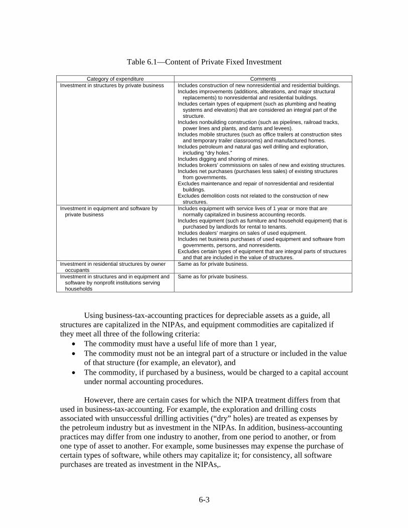
Table 6.1—Content of Private Fixed Investment
Category of expenditure Comments
Investment in structures by private business Includes construction of new nonresidential and residential buildings. Includes improvements (additions, alterations, and major structural
replacements) to nonresidential and residential buildings. Includes certain types of equipment (such as plumbing and heating
systems and elevators) that are considered an integral part of the structure.
Includes nonbuilding construction (such as pipelines, railroad tracks, power lines and plants, and dams and levees).
Includes mobile structures (such as office trailers at construction sites and temporary trailer classrooms) and manufactured homes.
Includes petroleum and natural gas well drilling and exploration, including “dry holes.”
Includes digging and shoring of mines. Includes brokers’ commissions on sales of new and existing structures. Includes net purchases (purchases less sales) of existing structures
from governments. Excludes maintenance and repair of nonresidential and residential
buildings. Excludes demolition costs not related to the construction of new
structures. Investment in equipment and software by
private business Includes equipment with service lives of 1 year or more that are
normally capitalized in business accounting records. Includes equipment (such as furniture and household equipment) that is
purchased by landlords for rental to tenants. Includes dealers’ margins on sales of used equipment. Includes net business purchases of used equipment and software from
governments, persons, and nonresidents. Excludes certain types of equipment that are integral parts of structures
and that are included in the value of structures. Investment in residential structures by owner
occupants Same as for private business.
Investment in structures and in equipment and software by nonprofit institutions serving households
Same as for private business.
Using business-tax-accounting practices for depreciable assets as a guide, all structures are capitalized in the NIPAs, and equipment commodities are capitalized if they meet all three of the following criteria:
• The commodity must have a useful life of more than 1 year, • The commodity must not be an integral part of a structure or included in the value
of that structure (for example, an elevator), and • The commodity, if purchased by a business, would be charged to a capital account
under normal accounting procedures. However, there are certain cases for which the NIPA treatment differs from that used in business-tax-accounting. For example, the exploration and drilling costs associated with unsuccessful drilling activities (“dry” holes) are treated as expenses by the petroleum industry but as investment in the NIPAs. In addition, business-accounting practices may differ from one industry to another, from one period to another, or from one type of asset to another. For example, some businesses may expense the purchase of certain types of software, while others may capitalize it; for consistency, all software purchases are treated as investment in the NIPAs,.
6-3
These capitalization rules and the selection of commodities that are treated as fixed assets are reviewed and updated during the preparation of BEA’s benchmark input-output (I-O) accounts. Additionally, during a comprehensive revision of the NIPAs, when the estimates from the most recent I-O benchmark are incorporated, BEA may change its treatment of certain types of structures and of equipment and software.5 The NIPA measure of PFI records capital expenditures on structures in the United States regardless of whether the structure is U.S.-owned or foreign-owned.6 It records capital expenditures on equipment and software in the United States regardless of whether the equipment and software are domestically produced or imported. In contrast, capital expenditures by U.S. residents on structures in other countries and U.S. exports of equipment and software are excluded from the PFI measure. In the NIPAs, the broadest measure of PFI is gross private fixed investment. It is measured without deduction of consumption of fixed capital (CFC), which is a measure of capital used up in production. Gross private fixed investment less CFC equals net private fixed investment. Gross private fixed investment comprises nonresidential fixed investment in structures and in equipment and software and residential fixed investment in structures and equipment. Nonresidential structures consists of new construction—including own-account construction;7 improvements to existing structures;8 expenditures on new mobile structures; expenditures on mining exploration, shafts, and wells; brokers’ commissions on sales of structures;9 and net purchases of used structures by private businesses and by nonprofit institutions from government agencies.10 In addition, it includes equipment that
5 For instance, as a result of technological and institutional changes and of revisions to international guidelines, some items that were once treated as current expenditures in the NIPAs are now capitalized. These items include software, nuclear fuel rods, drilling costs and construction of mine shafts, major replacements to residential structures and to railroad tracks, construction of manufactured homes and other mobile structures, and major appliances installed in tenant-occupied units. Conversely, small tools (such as an auto mechanic’s toolbox) that were once capitalized in the NIPAs are now expensed. As part of the upcoming 2013 comprehensive revision, BEA is planning to incorporate research and development spending as investment into its core accounts. In addition, BEA is exploring the feasibility of creating satellite accounts that would report investment in a variety of other intangible assets, such as individuals’ investments in human capital (see Ana Aizcorbe, Carol E. Moylan, and Carol A. Robbins, “BEA Briefing: Toward Better Measurement of Innovation and Intangibles,” Survey of Current Business 89 (January 2009): 10–23). 6 Ownership of a structure in a country signifies a long-term economic interest in that country, and thus the owner is considered a resident of that country. 7 For nonresidential fixed investment, own-account construction consists of the value of construction materials supplied by the project owner and the value of the labor supplied by the owner’s own construction employees assigned to the project. 8 Improvements to nonresidential structures are included with new construction but are not separately identified. 9 These commissions are considered part of the total price paid by the purchaser for the structure and thus are counted as part of the value of investment. 10 These transactions are included so that private and government ownership of the net stock of fixed assets is properly recorded; by definition, such transfers net to zero and do not affect gross domestic product.
6-4
is considered to be an integral part of the structure (such as plumbing, heating, and electrical systems). Nonresidential equipment and software consists of purchases by private businesses and by nonprofit institutions of new equipment (such as machinery, furniture, and motor vehicles) and of computer software that meet the above definition of a fixed asset. It also includes dealers’ margins on sales of used equipment to businesses and to nonprofit institutions; net purchases of used equipment from government agencies, from persons, and from the rest of the world; and own-account production of equipment and software. It is measured net of the value of worn out equipment sold for scrap. Residential structures consists of new construction of permanent-site single-family and multifamily housing units, improvements (additions, alterations, and major structural replacements) to housing units,11 expenditures on manufactured homes, brokers’ commissions on the sale of residential property, and net purchases of used structures from government agencies. Residential structures also includes some types of equipment (such as heating and air conditioning equipment) that are built into the structure. Residential equipment consists of equipment, such as furniture or household appliances, that is purchased by landlords for rental to tenants.
Recording in the NIPAs As described in chapter 2, the NIPAs can be viewed as aggregations of accounts belonging to individual transactors in the economy. PFI represents the final demand for structures and for equipment and software by private businesses and by other entities that are treated similarly to businesses in the NIPAs. In the seven summary accounts of the NIPAs, PFI appears in the Domestic Income and Product Account (account 1) as the dominant component of gross private domestic investment and in the Domestic Capital Account (account 6) as the dominant component of gross domestic investment. In the NIPAs, PFI is shown by type of product classification rather than by industry classification. Annual estimates of gross fixed investment and net fixed investment (that is, investment less CFC) by major type are provided in NIPA table group 5.2. PFI by type is presented in NIPA table group 5.3. PFI in structures by type is shown
11 Improvements to residential structures—which, unlike those to nonresidential structures, are shown separately in the NIPAs—consist of additions, alterations, and major replacements to structures subsequent to their completion. They include construction of additional housing units in existing residential structures, finishing of basements and attics, remodeling of kitchens and bathrooms, and the addition of swimming pools and garages. They include major replacements—such as new roofs, water heaters, furnaces, and central air conditioners—that prolong the expected life of the structure or add to its value; routine maintenance and repair work is not included. For residential fixed investment, own-account construction (“do-it-yourself” projects) consists of the value of the materials supplied only and does not include the value of the labor supplied by the property owner.
6-5
in table group 5.4, and PFI in equipment and software by type is shown in table group 5.5. The following is a list of the principal NIPA tables that present the PFI estimates: 5.2.3 Real Gross and Net Domestic Investment by Major Type, Quantity Indexes 5.2.5 Gross and Net Domestic Investment by Major Type 5.2.6 Real Gross and Net Domestic Investment by Major Type, Chained Dollars 5.3.1 Percent Change From Preceding Period in Real Private Fixed Investment by Type 5.3.2 Contributions to Percent Change in Real Private Fixed Investment by Type 5.3.3 Real Private Fixed Investment by Type, Quantity Indexes 5.3.4 Price Indexes for Private Fixed Investment by Type 5.3.5 Private Fixed Investment by Type 5.3.6 Real Private Fixed Investment by Type, Chained Dollars 5.4.1 Percent Change From Preceding Period in Real Private Fixed Investment in
Structures by Type 5.4.2 Contributions to Percent Change in Real Private Fixed Investment in Structures
by Type 5.4.3 Real Private Fixed Investment in Structures by Type, Quantity Indexes 5.4.4 Price Indexes for Private Fixed Investment in Structures by Type 5.4.5 Private Fixed Investment in Structures by Type 5.4.6 Real Private Fixed Investment in Structures by Type, Chained Dollars 5.5.1 Percent Change From Preceding Period in Real Private Fixed Investment in
Equipment and Software by Type 5.5.2 Contributions to Percent Change in Real Private Fixed Investment in Equipment
and Software by Type 5.5.3 Real Private Fixed Investment in Equipment and Software by Type, Quantity
Indexes 5.5.4 Price Indexes for Private Fixed Investment in Equipment and Software by Type 5.5.5 Private Fixed Investment in Equipment and Software by Type 5.5.6 Real Private Fixed Investment in Equipment and Software by Type, Chained
Dollars BEA also prepares “Underlying Detail” tables for PFI that provide current-dollar, chained-dollar, and price estimates at a greater level of detail than are shown in the above tables. BEA does not include these detailed estimates in the published tables because their quality is significantly less than that of the higher level categories of which they are a part. In particular, the detailed estimates are more likely to be based on judgmental trends, on trends in the higher level category, or on less reliable source data. The underlying detail tables for PFI consist of tables that provide quarterly estimates that are in the same format as, and consistent with, the annual estimates shown in NIPA table groups 5.2, 5.4, and 5.5. In addition, estimates of PFI by industry and by legal form of organization are presented as part of BEA’s fixed assets and consumer durable goods accounts.12 12 Go to www.bea.gov/national/FA2004/index.asp.
6-6
Overview of Source Data and Estimating Methods
As described earlier, the NIPA estimates, including those for PFI, are prepared using a wide variety of source data (see “Chapter 3: Principal Source Data”) and using estimating methods that adjust the source data to the required NIPA concepts and that fill in gaps in coverage and timing (see “Chapter 4: Estimating Methods”). For PFI, the estimates are based on government statistical reports, primarily from the U.S. Bureau of the Census but also from other federal government agencies, and on reports from private organizations, such as trade associations. The following are among the principal source data used for the PFI estimates: BEA’s benchmark I-O accounts, which are primarily based on the Census Bureau’s economic censuses, and BEA’s international transactions accounts; the Census Bureau’s annual and monthly surveys of manufacturers, monthly construction statistics, and monthly foreign trade data; and the Bureau of Labor Statistics’ (BLS) producer price indexes (PPIs) and import price indexes. Table 6.A (investment in structures) and table 6.B (investment in equipment and software) at the end of this chapter summarize the source data and estimating methods that are used to prepare the current-dollar benchmark, nonbenchmark, and current quarterly estimates and the quantity and price indexes for the detailed categories shown by type in NIPA table groups 5.4 and 5.5. Benchmark-year estimates For benchmark years, BEA’s benchmark I-O accounts are used to establish the levels of PFI and its components. The I-O accounts show the domestic output of each commodity and its disposition—either as intermediate consumption by industries or as purchases for final use, including business investment. In the I-O accounts, PFI is presented as the sum of detailed commodities purchased by business for final use.13 These commodities are then grouped into the PFI categories shown in the NIPA tables.14
For structures, the benchmark I-O estimates are primarily based on detailed value-
put-in-place data from the Census Bureau’s monthly survey of construction spending. The “value of construction put in place” is defined as the value of construction installed or erected at the construction site during a given period, regardless of when the work on the project was started or completed, when the structure was sold or delivered, or when payment for the structure was made.15 BEA adjusts the value-put-in-place data to account
13 For more information on the preparation of the I-O benchmark accounts, see U.S. Bureau of Economic Analysis, Concepts and Methods of the U.S. Input-Output Accounts, September 2006, at http://www.bea.gov/papers/IOmanual_092906.pdf. 14 A complete listing of the commodities underlying each category of PFI in equipment and software is available at http://www.bea.gov/faq/industry/IOCompPESv1.xls. 15 Value put in place is measured as the sum of the cost of materials installed or erected; cost of labor supplied by contractors and by project owners; and a proportionate share of the cost of construction equipment rental, contractors’ profit, cost of architectural and engineering work, miscellaneous overhead
6-7
for coverage gaps that are implied by comparing these data with those from the Census Bureau’s economic census.16 In addition, BEA uses data from other government sources and from trade sources in estimating the following structures categories: mobile structures; oil and natural gas well drilling and exploration; other mining exploration, shafts, and wells; residential manufactured homes; brokers’ commissions on the sale of structures; and net purchases of used structures from government agencies.
For equipment and software, the benchmark estimates are largely prepared using
the commodity-flow method (for a general description of this method, see “Commodity-flow method” in chapter 4). This method, which is implemented in its most complete form in preparing the benchmark I-O accounts, generally begins with a value of domestic output (principally manufacturers’ shipments) based on detailed data from the economic censuses. Next, the domestic supply of each commodity—the amount available for domestic consumption—is estimated by adding imports and subtracting exports, both based on the Census Bureau’s international trade data. The domestic supply is then allocated among domestic purchasers—business, government, and consumers. For most commodities, the allocation of purchases to business, and the subsequent allocation of those purchases between intermediate and final use, is based on economic census data. In a few cases, the allocation is entirely to final use (for example, motor vehicles) or to intermediate use (for example, semiconductors).17 The commodity-flow calculations also include estimates of trade margins and transportation costs18 and estimates of transactions in used equipment (see the technical note at the end of this chapter).
The following estimates are prepared directly rather than by commodity flow:
installation costs for communication equipment, industrial process design costs, and expenditures for nuclear fuel rods, for scrap metal, and for own-account software (for a description of the estimation procedure for investment in own-account software, see the technical note). Nonbenchmark-year estimates The estimates of structures for nonbenchmark years are generally prepared at the same level of detail as those for benchmark years. For most components, the estimates are prepared by using the monthly construction spending data as an indicator series to extrapolate the benchmark-year estimates (see “Interpolation and extrapolation using an indicator series” in chapter 4) and by assuming that the relationships underlying the benchmark estimates remain unchanged. For example, the coverage adjustments made to
and office costs chargeable to the project on the owners’ books, and interest and taxes paid during construction. 16 These adjustments are for own-account construction, for small projects that are excluded from the value-put-in-place data, and for nonresidential improvements. 17 For a description of the methodology used to prepare the estimates for new motor vehicles, see the technical note in “Chapter 5: Personal Consumption Expenditures.” 18 Trade margins measure the cost of marketing goods from producers to final purchasers, including markups by wholesalers and retailers. Transportation costs measure the costs of carrying goods by rail, truck, water, air, and liquid and gas pipelines.
6-8

the construction spending data for the benchmark year are assumed to be a constant proportion for periods after the benchmark year until the next benchmark estimates are available. The estimates of equipment and software for nonbenchmark years are generally prepared at a more aggregate level of detail than those for benchmark years, primarily because data on shipments are not available for the detailed product groupings. For most components, the estimates are prepared using an abbreviated form of the commodity-flow method that accommodates the available source data. For years except the most recent year, the primary source for domestic manufacturers’ shipments is the Census Bureau’s annual survey of manufactures (ASM), which collects data by product class; for the most recent year, the primary source for shipments is the Census Bureau’s monthly survey of manufacturers’ shipments, inventories, and orders, which collects data by industry group. For most components, estimates of exports and imports (based on international trade data), government purchases (based on Federal agency administrative data and on Census Bureau surveys of state and local government finance), and inventories (based on Census Bureau surveys and on IRS tabulations of business tax returns) are available. The estimates of the distributions of purchases among consumers, business final use, and business intermediate purchases are largely based on the benchmark relationships. Current quarterly estimates The current-dollar quarterly estimates—that is, the estimates for the quarters that have not yet been subject to an annual revision—for most categories of structures are prepared by extrapolation, using the same data sources as those used for the nonbenchmark-year estimates. For net purchases of used structures, the current quarterly estimates are based on judgmental trends. For petroleum and natural gas exploration and drilling, the quantity estimates for the current quarter are prepared first by extrapolating the quantity annual series using indicator series; these estimates are then converted (reflated) to current-dollar values using quarterly price indexes (see the technical note at the end of this chapter). The current quarterly estimates for equipment and software are prepared by the abbreviated commodity-flow method at the same aggregated level and based on the same data source as that used for the most-recent-year estimates (chart 6.1).
6-9
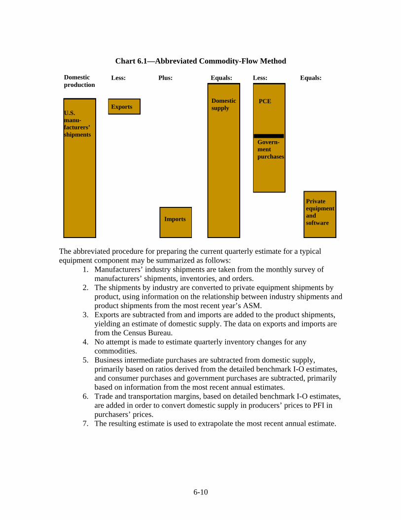
Chart 6.1—Abbreviated Commodity-Flow Method
Domestic production
Equals: Plus: Less: Less: Equals: Domestic
supply PCE
Exports U.S. manu-facturers’ shipments
Govern-ment purchases
Private
equipment and software
Imports The abbreviated procedure for preparing the current quarterly estimate for a typical equipment component may be summarized as follows:
1. Manufacturers’ industry shipments are taken from the monthly survey of manufacturers’ shipments, inventories, and orders.
2. The shipments by industry are converted to private equipment shipments by product, using information on the relationship between industry shipments and product shipments from the most recent year’s ASM.
3. Exports are subtracted from and imports are added to the product shipments, yielding an estimate of domestic supply. The data on exports and imports are from the Census Bureau.
4. No attempt is made to estimate quarterly inventory changes for any commodities.
5. Business intermediate purchases are subtracted from domestic supply, primarily based on ratios derived from the detailed benchmark I-O estimates, and consumer purchases and government purchases are subtracted, primarily based on information from the most recent annual estimates.
6. Trade and transportation margins, based on detailed benchmark I-O estimates, are added in order to convert domestic supply in producers’ prices to PFI in purchasers’ prices.
7. The resulting estimate is used to extrapolate the most recent annual estimate.
6-10
6-11
Quantity and price estimates The estimates of quantities purchased, or real spending, for most of the detailed PFI categories are prepared by deflation. Under this method, the quantities are calculated by dividing the current-dollar value of the component by an “appropriate” price index (with the reference year set equal to 100). For petroleum and natural gas exploration and drilling, the quantity estimates are prepared by direct valuation (see the technical note). (For a general description of these methods, see “Estimates for detailed components” in chapter 4.)
For structures, a wide variety of price indexes from public and private sources are used as deflators. For some components of nonresidential structures, quality-adjusted output price measures, such as PPIs, are not available, and BEA uses combinations of input-cost measures and output-cost measures in an effort to capture productivity and quality changes.19 For most equipment categories, detailed PPIs and import price indexes from BLS are used. The aggregate PFI measures are calculated from the detailed components as chain-type quantity and price indexes (for information about these calculations, see “Estimates for NIPA aggregates” in chapter 4). BEA also prepares measures of real PFI and its components in a dollar-denominated form, designated “chained-dollar” estimates (see “Chained-dollar measures” in chapter 4).20
19 For more information, see Paul R. Lally, “BEA Briefing: How BEA Accounts for Investment in Private Structures,” Survey 89 (February 2009): 11. 20 BEA does not provide chained-dollar measures (as distinct from chain-weighted indexes and percent changes) for computers, which are affected by highly volatile changes in prices and quantities (see J. Steven Landefeld, Brent R. Moulton, and Cindy M. Vojtech, “Chained-Dollar Indexes: Issues, Tips on Their Use, and Upcoming Changes,” Survey 83 (November 2003): 16.
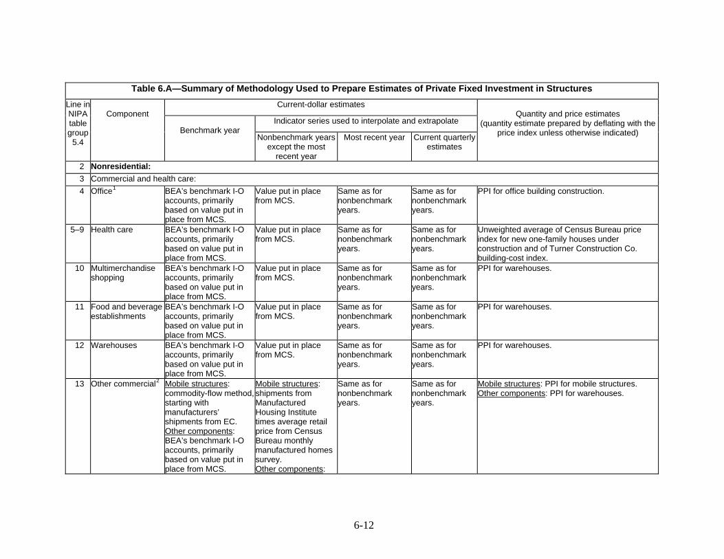
Table 6.A—Summary of Methodology Used to Prepare Estimates of Private Fixed Investment in Structures Current-dollar estimates
Indicator series used to interpolate and extrapolate
Line in NIPA table group
5.4
Component
Benchmark year
Nonbenchmark years except the most
recent year
Most recent year
Current quarterly estimates
Quantity and price estimates
(quantity estimate prepared by deflating with the price index unless otherwise indicated)
2 Nonresidential: 3 Commercial and health care: 4 Office1 BEA’s benchmark I-O
accounts, primarily based on value put in place from MCS.
Value put in place from MCS.
Same as for nonbenchmark years.
Same as for nonbenchmark years.
PPI for office building construction.
5–9 Health care BEA’s benchmark I-O accounts, primarily based on value put in place from MCS.
Value put in place from MCS.
Same as for nonbenchmark years.
Same as for nonbenchmark years.
Unweighted average of Census Bureau price index for new one-family houses under construction and of Turner Construction Co. building-cost index.
10 Multimerchandise shopping
BEA’s benchmark I-O accounts, primarily based on value put in place from MCS.
Value put in place from MCS.
Same as for nonbenchmark years.
Same as for nonbenchmark years.
PPI for warehouses.
11 Food and beverage establishments
BEA’s benchmark I-O accounts, primarily based on value put in place from MCS.
Value put in place from MCS.
Same as for nonbenchmark years.
Same as for nonbenchmark years.
PPI for warehouses.
12 Warehouses BEA’s benchmark I-O accounts, primarily based on value put in place from MCS.
Value put in place from MCS.
Same as for nonbenchmark years.
Same as for nonbenchmark years.
PPI for warehouses.
13 Other commercial2 Mobile structures: commodity-flow method, starting with manufacturers’ shipments from EC. Other components: BEA’s benchmark I-O accounts, primarily based on value put in place from MCS.
Mobile structures: shipments from Manufactured Housing Institute times average retail price from Census Bureau monthly manufactured homes survey. Other components:
Same as for nonbenchmark years.
Same as for nonbenchmark years.
Mobile structures: PPI for mobile structures. Other components: PPI for warehouses.
6-12
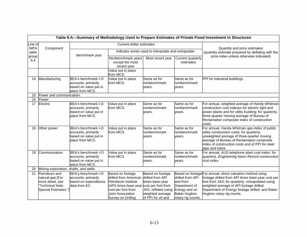
Table 6.A—Summary of Methodology Used to Prepare Estimates of Private Fixed Investment in Structures Current-dollar estimates
Indicator series used to interpolate and extrapolate
Line in NIPA table group
5.4
Component
Benchmark year
Nonbenchmark years except the most
recent year
Most recent year
Current quarterly estimates
Quantity and price estimates
(quantity estimate prepared by deflating with the price index unless otherwise indicated)
Value put in place from MCS.
14 Manufacturing BEA’s benchmark I-O accounts, primarily based on value put in place from MCS.
Value put in place from MCS.
Same as for nonbenchmark years.
Same as for nonbenchmark years.
PPI for industrial buildings.
15 Power and communication: 16 Power: 17 Electric BEA’s benchmark I-O
accounts, primarily based on value put in place from MCS.
Value put in place from MCS.
Same as for nonbenchmark years.
Same as for nonbenchmark years.
For annual, weighted average of Handy-Whitmanconstruction cost indexes for electric light and power plants and for utility building; for quarterly, three-quarter moving average of Bureau of Reclamation composite index of construction costs.
18 Other power BEA’s benchmark I-O accounts, primarily based on value put in place from MCS.
Value put in place from MCS.
Same as for nonbenchmark years.
Same as for nonbenchmark years.
For annual, Handy-Whitman gas index of public utility construction costs; for quarterly, unweighted average of three-quarter moving average of Bureau of Reclamation composite index of construction costs and of PPI for steel pipe and tubes.
19 Communication BEA’s benchmark I-O accounts, primarily based on value put in place from MCS.
Value put in place from MCS.
Same as for nonbenchmark years.
Same as for nonbenchmark years.
For annual, AUS telephone plant cost index; for quarterly, Engineering News Record construction cost index.
20 Mining exploration, shafts, and wells: 21 Petroleum and
natural gas [For more detail, see “Technical Note: Special Estimates.”]
BEA’s benchmark I-O accounts, primarily based on expenditures data from EC.
Based on footage drilled from American Petroleum Institute (API) times base-yearcost per foot from Joint Association Survey on Drilling
Based on footage drilled from API times base-year cost per foot from JAS, reflated using weighted average of PPI for oil and
Based on footage drilled from API and from Department of Energy and on Baker Hughes rotary rig counts,
For annual, direct valuation method using footage drilled from API times base-year cost per foot from JAS; for quarterly, extrapolated using weighted average of API footage drilled, Department of Energy footage drilled, and Baker Hughes rotary rig counts.
6-13
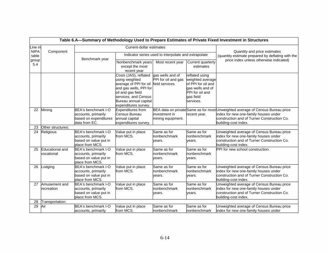
Table 6.A—Summary of Methodology Used to Prepare Estimates of Private Fixed Investment in Structures Current-dollar estimates
Indicator series used to interpolate and extrapolate
Line in NIPA table group
5.4
Component
Benchmark year
Nonbenchmark years except the most
recent year
Most recent year
Current quarterly estimates
Quantity and price estimates
(quantity estimate prepared by deflating with the price index unless otherwise indicated)
Costs (JAS), reflated using weighted average of PPI for oil and gas wells, PPI for oil and gas field services, and Census Bureau annual capital expenditures survey.
gas wells and of PPI for oil and gas field services.
reflated using weighted average of PPI for oil and gas wells and of PPI for oil and gas field services.
22 Mining BEA’s benchmark I-O accounts, primarily based on expenditures data from EC.
Expenditures from Census Bureau annual capital expenditures survey.
BEA data on private investment in mining equipment.
Same as for most recent year.
Unweighted average of Census Bureau price index for new one-family houses under construction and of Turner Construction Co. building-cost index.
23 Other structures: 24 Religious BEA’s benchmark I-O
accounts, primarily based on value put in place from MCS.
Value put in place from MCS.
Same as for nonbenchmark years.
Same as for nonbenchmark years.
Unweighted average of Census Bureau price index for new one-family houses under construction and of Turner Construction Co. building-cost index.
25 Educational and vocational
BEA’s benchmark I-O accounts, primarily based on value put in place from MCS.
Value put in place from MCS.
Same as for nonbenchmark years.
Same as for nonbenchmark years.
PPI for new school construction.
26 Lodging BEA’s benchmark I-O accounts, primarily based on value put in place from MCS.
Value put in place from MCS.
Same as for nonbenchmark years.
Same as for nonbenchmark years.
Unweighted average of Census Bureau price index for new one-family houses under construction and of Turner Construction Co. building-cost index.
27 Amusement and recreation
BEA’s benchmark I-O accounts, primarily based on value put in place from MCS.
Value put in place from MCS.
Same as for nonbenchmark years.
Same as for nonbenchmark years.
Unweighted average of Census Bureau price index for new one-family houses under construction and of Turner Construction Co. building-cost index.
28 Transportation: 29 Air BEA’s benchmark I-O
accounts, primarily Value put in place from MCS.
Same as for nonbenchmark
Same as for nonbenchmark
Unweighted average of Census Bureau price index for new one-family houses under
6-14
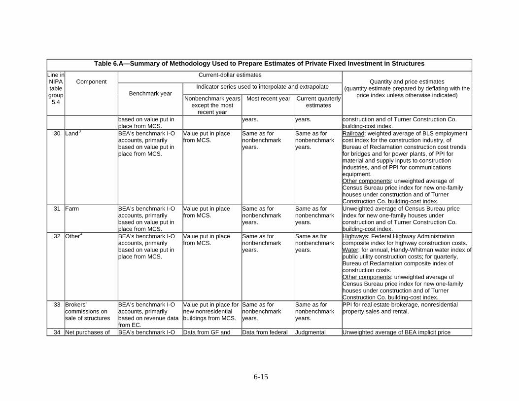
Table 6.A—Summary of Methodology Used to Prepare Estimates of Private Fixed Investment in Structures Current-dollar estimates
Indicator series used to interpolate and extrapolate
Line in NIPA table group
5.4
Component
Benchmark year
Nonbenchmark years except the most
recent year
Most recent year
Current quarterly estimates
Quantity and price estimates
(quantity estimate prepared by deflating with the price index unless otherwise indicated)
based on value put in place from MCS.
years. years. construction and of Turner Construction Co. building-cost index.
30 Land3 BEA’s benchmark I-O accounts, primarily based on value put in place from MCS.
Value put in place from MCS.
Same as for nonbenchmark years.
Same as for nonbenchmark years.
Railroad: weighted average of BLS employment cost index for the construction industry, of Bureau of Reclamation construction cost trends for bridges and for power plants, of PPI for material and supply inputs to construction industries, and of PPI for communications equipment. Other components: unweighted average of Census Bureau price index for new one-family houses under construction and of Turner Construction Co. building-cost index.
31 Farm BEA’s benchmark I-O accounts, primarily based on value put in place from MCS.
Value put in place from MCS.
Same as for nonbenchmark years.
Same as for nonbenchmark years.
Unweighted average of Census Bureau price index for new one-family houses under construction and of Turner Construction Co. building-cost index.
32 Other4 BEA’s benchmark I-O accounts, primarily based on value put in place from MCS.
Value put in place from MCS.
Same as for nonbenchmark years.
Same as for nonbenchmark years.
Highways: Federal Highway Administration composite index for highway construction costs. Water: for annual, Handy-Whitman water index of public utility construction costs; for quarterly, Bureau of Reclamation composite index of construction costs. Other components: unweighted average of Census Bureau price index for new one-family houses under construction and of Turner Construction Co. building-cost index.
33 Brokers’ commissions on sale of structures
BEA’s benchmark I-O accounts, primarily based on revenue data from EC.
Value put in place for new nonresidential buildings from MCS.
Same as for nonbenchmark years.
Same as for nonbenchmark years.
PPI for real estate brokerage, nonresidential property sales and rental.
34 Net purchases of BEA’s benchmark I-O Data from GF and Data from federal Judgmental Unweighted average of BEA implicit price
6-15
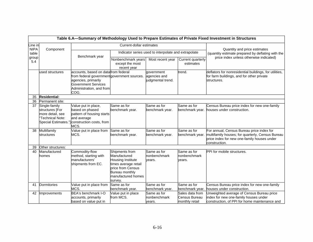
Table 6.A—Summary of Methodology Used to Prepare Estimates of Private Fixed Investment in Structures Current-dollar estimates
Indicator series used to interpolate and extrapolate
Line in NIPA table group
5.4
Component
Benchmark year
Nonbenchmark years except the most
recent year
Most recent year
Current quarterly estimates
Quantity and price estimates
(quantity estimate prepared by deflating with the price index unless otherwise indicated)
used structures accounts, based on data from federal government agencies, primarily Government Services Administration, and from COG.
from federal government sources.
government agencies and judgmental trend.
trend. deflators for nonresidential buildings, for utilities, for farm buildings, and for other private structures.
35 Residential: 36 Permanent site: 37 Single-family
structures [For more detail, see “Technical Note: Special Estimates.”]
Value put in place, based on phased pattern of housing starts and average construction costs, from MCS.
Same as for benchmark year.
Same as for benchmark year.
Same as for benchmark year.
Census Bureau price index for new one-family houses under construction.
38 Multifamily structures
Value put in place from MCS.
Same as for benchmark year.
Same as for benchmark year.
Same as for benchmark year.
For annual, Census Bureau price index for multifamily houses; for quarterly, Census Bureau price index for new one-family houses under construction.
39 Other structures: 40 Manufactured
homes Commodity-flow method, starting with manufacturers’ shipments from EC.
Shipments from Manufactured Housing Institute times average retail price from Census Bureau monthly manufactured homes survey.
Same as for nonbenchmark years.
Same as for nonbenchmark years.
PPI for mobile structures.
41 Dormitories Value put in place from MCS.
Same as for benchmark year.
Same as for benchmark year.
Same as for benchmark year.
Census Bureau price index for new one-family houses under construction.
42 Improvements BEA’s benchmark I-O accounts, primarily based on value put in
Value put in place from MCS.
Same as for nonbenchmark years.
Sales data from Census Bureau monthly retail
Unweighted average of Census Bureau price index for new one-family houses under construction, of PPI for home maintenance and
6-16
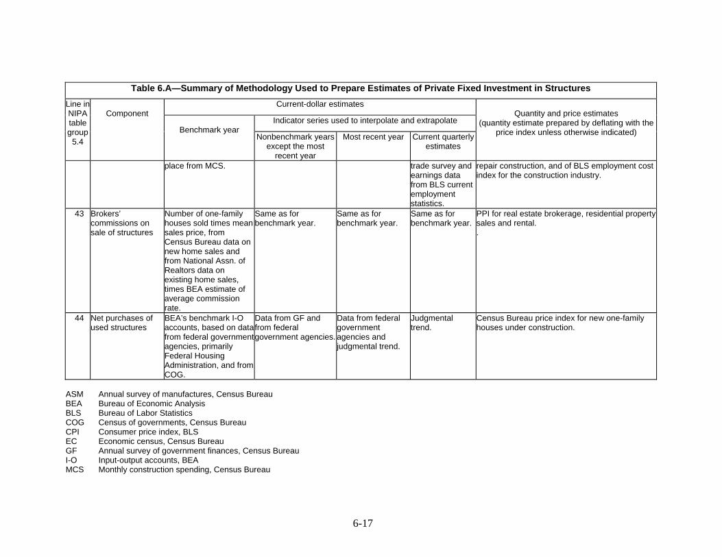
Table 6.A—Summary of Methodology Used to Prepare Estimates of Private Fixed Investment in Structures Current-dollar estimates
Indicator series used to interpolate and extrapolate
Line in NIPA table group
5.4
Component
Benchmark year
Nonbenchmark years except the most
recent year
Most recent year
Current quarterly estimates
Quantity and price estimates
(quantity estimate prepared by deflating with the price index unless otherwise indicated)
place from MCS. trade survey and earnings data from BLS current employment statistics.
repair construction, and of BLS employment cost index for the construction industry.
43 Brokers’ commissions on sale of structures
Number of one-family houses sold times mean sales price, from Census Bureau data on new home sales and from National Assn. of Realtors data on existing home sales, times BEA estimate of average commission rate.
Same as for benchmark year.
Same as for benchmark year.
Same as for benchmark year.
PPI for real estate brokerage, residential property sales and rental. .
44 Net purchases of used structures
BEA’s benchmark I-O accounts, based on data from federal government agencies, primarily Federal Housing Administration, and from COG.
Data from GF and from federal government agencies.
Data from federal government agencies and judgmental trend.
Judgmental trend.
Census Bureau price index for new one-family houses under construction.
ASM Annual survey of manufactures, Census Bureau BEA Bureau of Economic Analysis BLS Bureau of Labor Statistics COG Census of governments, Census Bureau CPI Consumer price index, BLS EC Economic census, Census Bureau GF Annual survey of government finances, Census Bureau I-O Input-output accounts, BEA MCS Monthly construction spending, Census Bureau
6-17
6-18
PPI Producer price index, BLS 1 Consists of office buildings, except those constructed at manufacturing sites and those constructed by power utilities for their own use. Includes all financial buildings. 2 Includes buildings and structures used by the retail, wholesale, and selected service industries. Consists of auto dealerships, garages, service stations, drug stores, restaurants, mobile structures, and other structures used for commercial purposes. Bus or truck garages are included in transportation. 3 Consists primarily of railroads. 4 Includes water supply, sewage and waste disposal, public safety, highway and street, and conservation and development.

Table 6.B—Summary of Methodology Used to Prepare Estimates of Private Fixed Investment in Equipment and Software Current-dollar estimates
Indicator series used to interpolate and extrapolate
Line in NIPA table group
5.5
Component
Benchmark year
Nonbenchmark years except the most
recent year
Most recent year
Current quarterly estimates
Quantity and price estimates
(quantity estimate prepared by deflating with the price index unless otherwise indicated)
2 Nonresidential equipment and software: 3 Information processing equipment and software: 4 Computers, software, and communication: 5 Computers and
peripheral equipment
Commodity-flow method, starting with manufacturers’ shipments from EC.
Abbreviated commodity-flow method, starting with manufacturers’ shipments from ASM.
Abbreviated commodity-flow method, starting with manufacturers’ shipments based on Federal Reserve Board industrial production index and on MSM.
Same as for most recent year.
PPI for host computers, multiusers, PPI for portablecomputers, laptops, PDAs, and other single user computers, PPI for personal computers and workstations (except portable computers), PPI for computer storage devices, PPI for computer terminals, and PPI for other computer peripheral equipment; IPI for computers, IPI for computer storage devices, IPI for computer displays, including monitors and terminals, and IPI for computer printers.
6 Software:1 Prepackaged
software Commodity-flow method, starting with industry receipts data from EC.
Abbreviated commodity-flow method, starting with industry receipts data from Census Bureau service annual survey.
Same as for nonbenchmark years.
For third estimate, QSS total revenue data; for second and advance estimates, receipts from company reports.
BEA price index based on PPI for application software publishing.
Custom software Commodity-flow method, starting with industry receipts data from EC.
Abbreviated commodity-flow method, starting with industry receipts data from Census Bureau service annual survey.
Same as for nonbenchmark years.
For third estimate, QSS total revenue data; for second and advance estimates, receipts from company reports.
Weighted average of the prepackaged software price and of an input-cost index based on BLS data on wage rates for computer programmers and systems analysts and on intermediate input costs associated with the production of software.
Own-account software [For more
Production costs based on BLS
Production costs based on BLS
Same as for nonbenchmark
Based on BLS current
Weighted average of the prepackaged software price and of an input-cost index based on BLS data
6-19
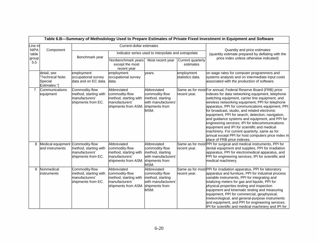
Table 6.B—Summary of Methodology Used to Prepare Estimates of Private Fixed Investment in Equipment and Software Current-dollar estimates
Indicator series used to interpolate and extrapolate
Line in NIPA table group
5.5
Component
Benchmark year
Nonbenchmark years except the most
recent year
Most recent year
Current quarterly estimates
Quantity and price estimates
(quantity estimate prepared by deflating with the price index unless otherwise indicated)
detail, see “Technical Note: Special Estimates.”]
employment occupational survey data and on EC data.
employment occupational survey data.
years. employment statistics data.
on wage rates for computer programmers and systems analysts and on intermediate input costs associated with the production of software.
7 Communications equipment
Commodity-flow method, starting with manufacturers’ shipments from EC.
Abbreviated commodity-flow method, starting with manufacturers’ shipments from ASM.
Abbreviated commodity-flow method, starting with manufacturers’ shipments from MSM.
Same as for most recent year.
For annual, Federal Reserve Board (FRB) price indexes for data networking equipment, telephone switching equipment, carrier line equipment, and wireless networking equipment; PPI for telephone apparatus, PPI for communications equipment, PPI for broadcast, studio, and related electronic equipment, PPI for search, detection, navigation, and guidance systems and equipment, and PPI for engineering services; IPI for telecommunications equipment and IPI for scientific and medical machinery. For current quarterly, same as for annual except PPI for host computers price index in place of FRB price indexes.
8 Medical equipment and instruments
Commodity-flow method, starting with manufacturers’ shipments from EC.
Abbreviated commodity-flow method, starting with manufacturers’ shipments from ASM.
Abbreviated commodity-flow method, starting with manufacturers’ shipments from MSM.
Same as for most recent year.
PPI for surgical and medical instruments, PPI for dental equipment and supplies, PPI for irradiation apparatus, PPI for electromedical apparatus, and PPI for engineering services; IPI for scientific and medical machinery.
9 Nonmedical instruments
Commodity-flow method, starting with manufacturers’ shipments from EC.
Abbreviated commodity-flow method, starting with manufacturers’ shipments from ASM.
Abbreviated commodity-flow method, starting with manufacturers’ shipments from MSM.
Same as for most recent year.
PPI for irradiation apparatus, PPI for laboratory apparatus and furniture, PPI for industrial process variable instruments, PPI for integrating and totalizing meters for gas and liquids, PPI for physical properties testing and inspection equipment and kinematic testing and measuring equipment, PPI for commercial, geophysical, meteorological, and general-purpose instruments and equipment, and PPI for engineering services; IPI for scientific and medical machinery and IPI for
6-20
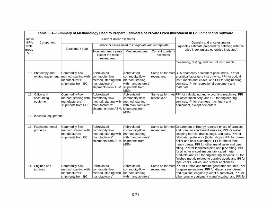
Table 6.B—Summary of Methodology Used to Prepare Estimates of Private Fixed Investment in Equipment and Software Current-dollar estimates
Indicator series used to interpolate and extrapolate
Line in NIPA table group
5.5
Component
Benchmark year
Nonbenchmark years except the most
recent year
Most recent year
Current quarterly estimates
Quantity and price estimates
(quantity estimate prepared by deflating with the price index unless otherwise indicated)
measuring, testing, and control instruments.
10 Photocopy and related equipment
Commodity-flow method, starting with manufacturers’ shipments from EC.
Abbreviated commodity-flow method, starting with manufacturers’ shipments from ASM.
Abbreviated commodity-flow method, starting with manufacturers’ shipments from MSM.
Same as for most recent year.
BEA photocopy equipment price index, PPI for analytical laboratory instruments, PPI for optical instruments and lenses, and PPI for engineering services; IPI for recreational equipment and materials.
11 Office and accounting equipment
Commodity-flow method, starting with manufacturers’ shipments from EC.
Abbreviated commodity-flow method, starting with manufacturers’ shipments from ASM.
Abbreviated commodity-flow method, starting with manufacturers’ shipments from MSM.
Same as for most recent year.
PPI for calculating and accounting machines, PPI for office machinery, and PPI for engineering services; IPI for business machinery and equipment, except computers.
12 Industrial equipment:
13 Fabricated metal products
Commodity-flow method, starting with manufacturers’ shipments from EC.
Abbreviated commodity-flow method, starting with manufacturers’ shipments from ASM.
Abbreviated commodity-flow method, starting with manufacturers’ shipments from MSM.
Same as for most recent year.
Department of Energy reported prices of uranium and uranium enrichment services, PPI for metal shipping barrels, drums, kegs, and pails, PPI for fabricated plate work (boiler shops), PPI for power boiler and heat exchanger, PPI for metal tank, heavy gauge, PPI for other metal valve and pipe fitting, PPI for fabricated pipe and pipe fitting, PPI for all other miscellaneous fabricated metal products, and PPI for engineering services; IPI for finished metals related to durable goods and IPI for taps, cocks, valves, and similar appliances.
14 Engines and turbines
Commodity-flow method, starting with manufacturers’ shipments from EC.
Abbreviated commodity-flow method, starting with manufacturers’
Abbreviated commodity-flow method, starting with manufacturers’
Same as for most recent year.
PPI for turbine and turbine generator set units, PPI for gasoline engines, PPI for diesel, semi-diesel, and dual fuel engines (except automotive), PPI for other engine equipment manufacturing, and PPI for
6-21
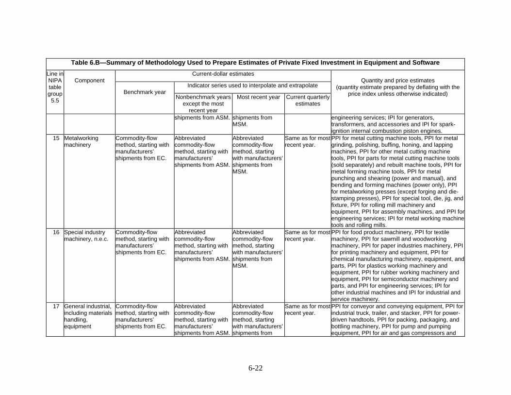
Table 6.B—Summary of Methodology Used to Prepare Estimates of Private Fixed Investment in Equipment and Software Current-dollar estimates
Indicator series used to interpolate and extrapolate
Line in NIPA table group
5.5
Component
Benchmark year
Nonbenchmark years except the most
recent year
Most recent year
Current quarterly estimates
Quantity and price estimates
(quantity estimate prepared by deflating with the price index unless otherwise indicated)
shipments from ASM. shipments from MSM.
engineering services; IPI for generators, transformers, and accessories and IPI for spark-ignition internal combustion piston engines.
15 Metalworking machinery
Commodity-flow method, starting with manufacturers’ shipments from EC.
Abbreviated commodity-flow method, starting with manufacturers’ shipments from ASM.
Abbreviated commodity-flow method, starting with manufacturers’ shipments from MSM.
Same as for most recent year.
PPI for metal cutting machine tools, PPI for metal grinding, polishing, buffing, honing, and lapping machines, PPI for other metal cutting machine tools, PPI for parts for metal cutting machine tools (sold separately) and rebuilt machine tools, PPI for metal forming machine tools, PPI for metal punching and shearing (power and manual), and bending and forming machines (power only), PPI for metalworking presses (except forging and die-stamping presses), PPI for special tool, die, jig, and fixture, PPI for rolling mill machinery and equipment, PPI for assembly machines, and PPI for engineering services; IPI for metal working machine tools and rolling mills.
16 Special industry machinery, n.e.c.
Commodity-flow method, starting with manufacturers’ shipments from EC.
Abbreviated commodity-flow method, starting with manufacturers’ shipments from ASM.
Abbreviated commodity-flow method, starting with manufacturers’ shipments from MSM.
Same as for most recent year.
PPI for food product machinery, PPI for textile machinery, PPI for sawmill and woodworking machinery, PPI for paper industries machinery, PPI for printing machinery and equipment, PPI for chemical manufacturing machinery, equipment, and parts, PPI for plastics working machinery and equipment, PPI for rubber working machinery and equipment, PPI for semiconductor machinery and parts, and PPI for engineering services; IPI for other industrial machines and IPI for industrial and service machinery.
17 General industrial, including materials handling, equipment
Commodity-flow method, starting with manufacturers’ shipments from EC.
Abbreviated commodity-flow method, starting with manufacturers’ shipments from ASM.
Abbreviated commodity-flow method, starting with manufacturers’ shipments from
Same as for most recent year.
PPI for conveyor and conveying equipment, PPI for industrial truck, trailer, and stacker, PPI for power-driven handtools, PPI for packing, packaging, and bottling machinery, PPI for pump and pumping equipment, PPI for air and gas compressors and
6-22

Table 6.B—Summary of Methodology Used to Prepare Estimates of Private Fixed Investment in Equipment and Software Current-dollar estimates
Indicator series used to interpolate and extrapolate
Line in NIPA table group
5.5
Component
Benchmark year
Nonbenchmark years except the most
recent year
Most recent year
Current quarterly estimates
Quantity and price estimates
(quantity estimate prepared by deflating with the price index unless otherwise indicated)
MSM. vacuum pumps, PPI for industrial spraying equipment, PPI for industrial and commercial fan and blower, PPI for air purification equipment, PPI for industrial process furnaces and ovens and industrial electrical heating equipment, PPI for scale and balance, except laboratory, equipment, PPI for welding and soldering equipment, and PPI for engineering services; IPI for oil drilling, mining, and construction machinery, IPI for metal working machine tools and rolling mills, and IPI for industrial and service machinery.
18 Electrical transmission, distribution, and industrial apparatus
Commodity-flow method, starting with manufacturers’ shipments from EC.
Abbreviated commodity-flow method, starting with manufacturers’ shipments from ASM.
Abbreviated commodity-flow method, starting with manufacturers’ shipments from MSM.
Same as for most recent year.
PPI for electrical measuring and integrating instruments, PPI for electric power and specialty transformer, PPI for switchgear and switchboard apparatus, PPI for motors and generators, PPI for relay and industrial control equipment, PPI for semiconductor power conversion apparatus, and PPI for engineering services; IPI for nonelectrical machinery, IPI for electric generating equipment, and IPI for electric apparatus and parts, n.e.c.
19 Transportation equipment: 20 Trucks, buses, and truck trailers: 21 Light trucks
(including utility vehicles)2 [For more detail, see the technical note to “Chapter 5: Personal Consumption Expenditures.”]
Based on unit sales from Wards’ Automotive Reports and registration data from R.L. Polk & Co. times average sales price from J.D. Power and Assoc.
Same as for benchmark year.
Same as for benchmark year.
Same as for benchmark year.
CPI for new trucks.
6-23
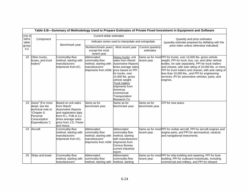
Table 6.B—Summary of Methodology Used to Prepare Estimates of Private Fixed Investment in Equipment and Software Current-dollar estimates
Indicator series used to interpolate and extrapolate
Line in NIPA table group
5.5
Component
Benchmark year
Nonbenchmark years except the most
recent year
Most recent year
Current quarterly estimates
Quantity and price estimates
(quantity estimate prepared by deflating with the price index unless otherwise indicated)
22 Other trucks, buses, and truck trailers2
Commodity-flow method, starting with manufacturers’ shipments from EC.
Abbreviated commodity-flow method, starting with manufacturers’ shipments from ASM.
Heavy trucks: unit sales from Wards’ Automotive Reportstimes average sales price based on PPI for trucks, over 14,000 lbs. gross vehicle weight. Truck trailers: shipments from Americas Commercial Transportation Research Co.
Same as for most recent year.
PPI for trucks, over 14,000 lbs. gross vehicle weight, PPI for truck, bus, car, and other vehicle bodies, for sale separately, PPI for truck trailers and chassis, with axle rating of 10,000 lbs. or more, PPI for truck trailers and chassis, with axle rating of less than 10,000 lbs., and PPI for engineering services; IPI for automotive vehicles, parts, and engines.
23 Autos2 [For more detail, see the technical note to “Chapter 5: Personal Consumption Expenditures.”]
Based on unit sales from Wards’ Automotive Reports and registration data from R.L. Polk & Co. times average sales price from J.D. Power and Assoc.
Same as for benchmark year.
Same as for benchmark year.
Same as for benchmark year.
CPI for new autos.
24 Aircraft Commodity-flow method, starting with manufacturers’ shipments from EC.
Abbreviated commodity-flow method, starting with manufacturers’ shipments from ASM
Abbreviated commodity-flow method, starting with manufacturers’ shipments from Census Bureau current industrial report.
Same as for most recent year.
PPI for civilian aircraft, PPI for aircraft engines and engine parts, and PPI for aeronautical, nautical, and navigational instruments.
25 Ships and boats Commodity-flow method, starting with manufacturers’
Abbreviated commodity-flow method, starting with
Abbreviated commodity-flow method, starting
Same as for most recent year.
PPI for ship building and repairing, PPI for boat building, PPI for outboard motorboats, including commercial and military, and PPI for inboard
6-24
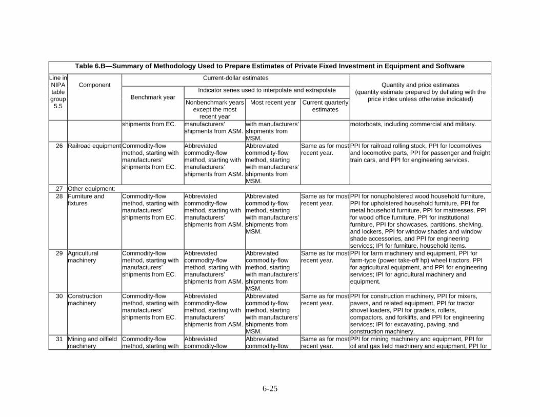
Table 6.B—Summary of Methodology Used to Prepare Estimates of Private Fixed Investment in Equipment and Software Current-dollar estimates
Indicator series used to interpolate and extrapolate
Line in NIPA table group
5.5
Component
Benchmark year
Nonbenchmark years except the most
recent year
Most recent year
Current quarterly estimates
Quantity and price estimates
(quantity estimate prepared by deflating with the price index unless otherwise indicated)
shipments from EC. manufacturers’ shipments from ASM.
with manufacturers’ shipments from MSM.
motorboats, including commercial and military.
26 Railroad equipment Commodity-flow method, starting with manufacturers’ shipments from EC.
Abbreviated commodity-flow method, starting with manufacturers’ shipments from ASM.
Abbreviated commodity-flow method, starting with manufacturers’ shipments from MSM.
Same as for most recent year.
PPI for railroad rolling stock, PPI for locomotives and locomotive parts, PPI for passenger and freight train cars, and PPI for engineering services.
27 Other equipment: 28 Furniture and
fixtures Commodity-flow method, starting with manufacturers’ shipments from EC.
Abbreviated commodity-flow method, starting with manufacturers’ shipments from ASM.
Abbreviated commodity-flow method, starting with manufacturers’ shipments from MSM.
Same as for most recent year.
PPI for nonupholstered wood household furniture, PPI for upholstered household furniture, PPI for metal household furniture, PPI for mattresses, PPI for wood office furniture, PPI for institutional furniture, PPI for showcases, partitions, shelving, and lockers, PPI for window shades and window shade accessories, and PPI for engineering services; IPI for furniture, household items.
29 Agricultural machinery
Commodity-flow method, starting with manufacturers’ shipments from EC.
Abbreviated commodity-flow method, starting with manufacturers’ shipments from ASM.
Abbreviated commodity-flow method, starting with manufacturers’ shipments from MSM.
Same as for most recent year.
PPI for farm machinery and equipment, PPI for farm-type (power take-off hp) wheel tractors, PPI for agricultural equipment, and PPI for engineering services; IPI for agricultural machinery and equipment.
30 Construction machinery
Commodity-flow method, starting with manufacturers’ shipments from EC.
Abbreviated commodity-flow method, starting with manufacturers’ shipments from ASM.
Abbreviated commodity-flow method, starting with manufacturers’ shipments from MSM.
Same as for most recent year.
PPI for construction machinery, PPI for mixers, pavers, and related equipment, PPI for tractor shovel loaders, PPI for graders, rollers, compactors, and forklifts, and PPI for engineering services; IPI for excavating, paving, and construction machinery.
31 Mining and oilfield machinery
Commodity-flow method, starting with
Abbreviated commodity-flow
Abbreviated commodity-flow
Same as for most recent year.
PPI for mining machinery and equipment, PPI for oil and gas field machinery and equipment, PPI for
6-25
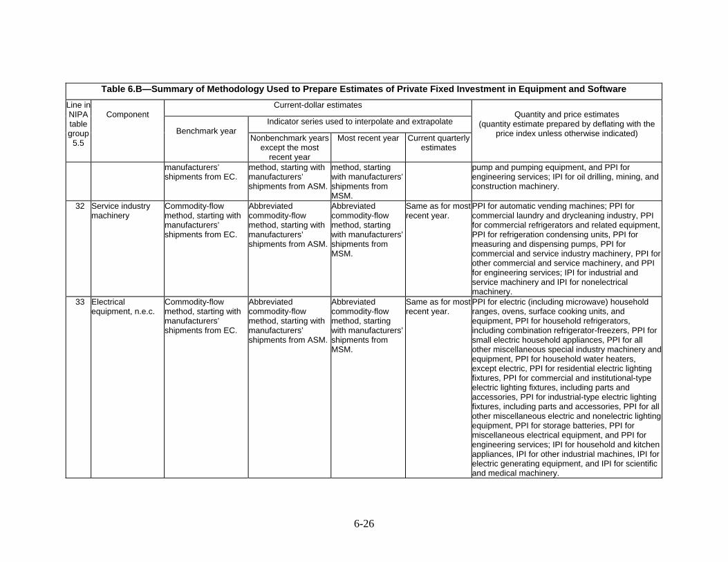
Table 6.B—Summary of Methodology Used to Prepare Estimates of Private Fixed Investment in Equipment and Software Current-dollar estimates
Indicator series used to interpolate and extrapolate
Line in NIPA table group
5.5
Component
Benchmark year
Nonbenchmark years except the most
recent year
Most recent year
Current quarterly estimates
Quantity and price estimates
(quantity estimate prepared by deflating with the price index unless otherwise indicated)
manufacturers’ shipments from EC.
method, starting with manufacturers’ shipments from ASM.
method, starting with manufacturers’ shipments from MSM.
pump and pumping equipment, and PPI for engineering services; IPI for oil drilling, mining, and construction machinery.
32 Service industry machinery
Commodity-flow method, starting with manufacturers’ shipments from EC.
Abbreviated commodity-flow method, starting with manufacturers’ shipments from ASM.
Abbreviated commodity-flow method, starting with manufacturers’ shipments from MSM.
Same as for most recent year.
PPI for automatic vending machines; PPI for commercial laundry and drycleaning industry, PPI for commercial refrigerators and related equipment, PPI for refrigeration condensing units, PPI for measuring and dispensing pumps, PPI for commercial and service industry machinery, PPI for other commercial and service machinery, and PPI for engineering services; IPI for industrial and service machinery and IPI for nonelectrical machinery.
33 Electrical equipment, n.e.c.
Commodity-flow method, starting with manufacturers’ shipments from EC.
Abbreviated commodity-flow method, starting with manufacturers’ shipments from ASM.
Abbreviated commodity-flow method, starting with manufacturers’ shipments from MSM.
Same as for most recent year.
PPI for electric (including microwave) household ranges, ovens, surface cooking units, and equipment, PPI for household refrigerators, including combination refrigerator-freezers, PPI for small electric household appliances, PPI for all other miscellaneous special industry machinery and equipment, PPI for household water heaters, except electric, PPI for residential electric lighting fixtures, PPI for commercial and institutional-type electric lighting fixtures, including parts and accessories, PPI for industrial-type electric lighting fixtures, including parts and accessories, PPI for all other miscellaneous electric and nonelectric lighting equipment, PPI for storage batteries, PPI for miscellaneous electrical equipment, and PPI for engineering services; IPI for household and kitchen appliances, IPI for other industrial machines, IPI for electric generating equipment, and IPI for scientific and medical machinery.
6-26
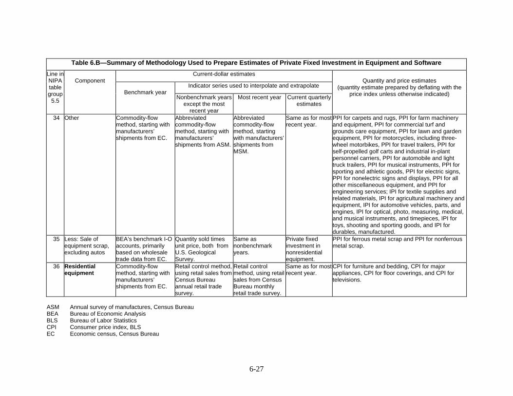
Table 6.B—Summary of Methodology Used to Prepare Estimates of Private Fixed Investment in Equipment and Software Current-dollar estimates
Indicator series used to interpolate and extrapolate
Line in NIPA table group
5.5
Component
Benchmark year
Nonbenchmark years except the most
recent year
Most recent year
Current quarterly estimates
Quantity and price estimates
(quantity estimate prepared by deflating with the price index unless otherwise indicated)
34 Other Commodity-flow method, starting with manufacturers’ shipments from EC.
Abbreviated commodity-flow method, starting with manufacturers’ shipments from ASM.
Abbreviated commodity-flow method, starting with manufacturers’ shipments from MSM.
Same as for most recent year.
PPI for carpets and rugs, PPI for farm machinery and equipment, PPI for commercial turf and grounds care equipment, PPI for lawn and garden equipment, PPI for motorcycles, including three-wheel motorbikes, PPI for travel trailers, PPI for self-propelled golf carts and industrial in-plant personnel carriers, PPI for automobile and light truck trailers, PPI for musical instruments, PPI for sporting and athletic goods, PPI for electric signs, PPI for nonelectric signs and displays, PPI for all other miscellaneous equipment, and PPI for engineering services; IPI for textile supplies and related materials, IPI for agricultural machinery and equipment, IPI for automotive vehicles, parts, and engines, IPI for optical, photo, measuring, medical, and musical instruments, and timepieces, IPI for toys, shooting and sporting goods, and IPI for durables, manufactured.
35 Less: Sale of equipment scrap, excluding autos
BEA’s benchmark I-O accounts, primarily based on wholesale trade data from EC.
Quantity sold times unit price, both from U.S. Geological Survey.
Same as nonbenchmark years.
Private fixed investment in nonresidential equipment.
PPI for ferrous metal scrap and PPI for nonferrous metal scrap.
36 Residential equipment
Commodity-flow method, starting with manufacturers’ shipments from EC.
Retail control method, using retail sales from Census Bureau annual retail trade survey.
Retail control method, using retail sales from Census Bureau monthly retail trade survey.
Same as for most recent year.
CPI for furniture and bedding, CPI for major appliances, CPI for floor coverings, and CPI for televisions.
ASM Annual survey of manufactures, Census Bureau BEA Bureau of Economic Analysis BLS Bureau of Labor Statistics CPI Consumer price index, BLS EC Economic census, Census Bureau
6-27
6-28
IPI Import price index, BLS MSM Monthly survey of manufacturers’ shipments, inventories, and orders, Census Bureau n.e.c. Not elsewhere classified PPI Producer price index, BLS QSS Quarterly service annual survey, Census Bureau 1 Excludes software “embedded,” or bundled, in computers and other equipment. 2 Includes net purchases of used vehicles.
Technical Note: Special Estimates
This section provides additional detail on the sources and methods used to
estimate the following key components of private fixed investment (PFI): petroleum and natural gas, new single-family structures, own-account software, and used equipment.
Petroleum and natural gas This PFI component includes all costs incurred in drilling oil and gas wells, regardless of whether the drilling activities were successful or unsuccessful.
For benchmark years, the current-dollar estimates of exploration expenditures and of all other drilling costs are prepared separately, based on data from the Census Bureau’s economic census.
For nonbenchmark years except the most recent year, the current-dollar estimates
are prepared by interpolation and extrapolation using indicator series.1 For estimates before 2006, the indicator series is based on data on footage drilled (onshore and offshore) from the American Petroleum Institute (API) and on data on the average cost per foot from a survey of drilling costs conducted by the API and the Independent Petroleum Association and published in the Joint Association Survey on Drilling Costs (JAS). Beginning with 2006, the estimates of exploration expenditures are prepared by reflating quantity estimates that are based on data on the count of seismic crews from the U.S. Department of Energy (DOE) using the PPI for oil and gas field services. Beginning with 2006, the estimates of all other drilling costs are based on API data on footage drilled times JAS data on base-year cost per foot, reflated using the PPIs for oil and gas well drilling and for oil and gas field services and data for the oil and gas extraction industry from the Census Bureau’s annual capital expenditures survey.
The current-dollar estimates for the most recent year and for the current quarters
are prepared by “reflating” the quantity estimates (described next) by multiplying them by a weighted average of the PPI for oil and gas well drilling and the PPI for oil and gas field services.
Quantity estimates. The annual estimates of real petroleum and natural gas well
drilling are prepared using the direct valuation method.2 The estimates of exploration expenditures are based on the DOE data on active seismic crews, and the estimates of all other drilling costs are based on API footage drilled and on the base-year average cost per foot from the JAS. The current quarterly estimates of real petroleum and natural gas well drilling are based on a weighted average of the API data on footage drilled, the DOE data on footage drilled, and data from Baker Hughes on rotary rig counts.
1 For a general description of this method, see the section “Interpolation and extrapolation using an indicator series” in “Chapter 4: Estimating Methods.” 2 For a general description of this method, see the section “Estimates for detailed components” in chapter 4.
6-29
New single-family structures
This PFI component measures the construction of fully detached units and of other units (such as rowhouses and townhouses) that are separated from adjacent units by a ground-to-roof wall and that do not share heating/air conditioning systems or other interstructural public utilities (such as water supply, power supply, or sewage disposal lines). The value of new single-family construction excludes the value of land, marketing costs, closing costs, and movable appliances. The annual and quarterly estimates of investment in new single-family structures are based on the Census Bureau’s monthly construction statistics on the value of new construction put in place for one-unit structures. The Census Bureau determines the construction cost of new single-family houses started each month using data from its monthly survey of new residential construction. Construction costs are estimated separately for units built to be sold or rented and for units built by an owner or for an owner on contract. The estimated cost of all single-family units started is then distributed into monthly value put in place by applying fixed 12-month patterns of monthly construction progress.3 The patterns vary somewhat depending on the particular month the unit is started; in general, the progress pattern assumes that about 16 percent of the project is completed in the first month, about 23 percent in the second month, about 20 percent in the third month, about 15 percent in the fourth month, about 10 percent in the fifth month, and the remainder is distributed in declining amounts over the succeeding 7 months.
For the advance current quarterly estimate, only 2 months of value-put-in-place data are available. BEA estimates the value put in place for the third month, primarily based on data on housing starts for that month and on the Census Bureau’s construction progress pattern.
Quantity estimates. The estimates of investment in real new single-family
structures are prepared by deflation, using the Census Bureau price index for new one-family houses under construction.
3 For more information, see “Construction Methodology” at http//:www.census.gov/const/C30/methodology.pdf.
6-30
Own-account software This PFI component measures the software that is produced by private businesses
for their own use.4 Own-account software consists of expenditures for new or significantly enhanced software that the business enterprise develops in-house rather than purchases from companies that are primarily engaged in software development. Own-account software includes the development of software originals from which copies are made for sale or incorporation into other products (such as motor vehicles or appliances), but it does not include the software copies.
The commodity-flow method is not used to prepare the estimates of expenditures
for own-account software. Instead, these expenditures are measured as the sum of production costs, which are limited to compensation (wage and nonwage) of employees and to the costs of intermediate inputs.
The estimates of wages for all years are derived by multiplying the number of
programmers and systems analysts in selected industries times the wage rate in those industries. Wages are reduced by half under the assumption that these programmers and analysts spend only about half their time working on the development of new or enhanced own-account software. In addition, wages are reduced by subtracting the portion of wages of programmers and analysts employed by the “computer systems design and related services industry” that represents the production of custom software for sale; sales of the custom software produced by this industry are already included in the PFI estimates of custom software. The data on the number of programmers and analysts by industry and the data on wages by occupation are from the BLS occupational employment statistics survey.
The estimates of nonwage compensation are based on relationships between wage
and nonwage compensation derived from NIPA data by industry. The estimates of input costs are based on relationships between intermediate inputs and compensation that are derived primarily from the Census Bureau’s economic census.
The estimates of expenditures for own-account software for the current quarters
are prepared by extrapolation, using an index of employment in four industries for which computer-related occupations account for a relatively high portion of total employment. The index is derived using BLS current employment data for computer systems design and related services; software publishers; data processing, hosting, and related services; and computer and peripheral equipment manufacturing.5
4 The treatment of business and government purchases of software and of own-account production of software as investment was introduced in the 1999 NIPA comprehensive revision; see Brent R. Moulton, Robert P. Parker, and Eugene P. Seskin, “A Preview of the Comprehensive Revision of the National Income and Product Accounts: Definitional and Classificational Changes,” Survey 79 (August 1999): 8–11. 5 This methodology was introduced in the 2010 annual revision of the NIPAs; see Eugene P. Seskin and Shelly Smith, “Annual Revision of the National Income and Product Accounts,” Survey 90 (August 2010): 22–23.
6-31

Quantity estimates. The estimates of real expenditures for own-account software are derived by deflation, using a weighted average of a BEA input-cost index and of a BEA price index for prepackaged software. The input-cost index is based on BLS data on wage rates for computer programmers and systems analysts and on a BEA index of intermediate input costs associated with the production of software. The prepackaged software price index is based on the PPI for application software publishing.
6-32
6-33
Used equipment Aside from trade margins and commissions earned by the services of brokers and
dealers, transactions in secondhand fixed assets among sectors do not reflect current production activity and so do not affect gross domestic product. However, these transfers of assets between sectors are recorded in the NIPAs so that the estimates of fixed investment are consistent with the estimates of the net stock of private fixed assets. Moreover, the estimates of saving by the individual sectors of the economy must reflect purchases of used equipment as well as purchases of new equipment. Thus, net purchases of used equipment by private business from households, governments, and the rest of the world are added to investment in equipment and software and are subtracted (as net sales) from personal consumption expenditures, from government fixed investment, and from net exports, respectively. Sales of used motor vehicles by business to persons account for the bulk of these intersectoral transactions; thus in the NIPAs, total net purchases of equipment by private business is negative. (For a detailed description of the methodology used to prepare the NIPA estimates for net purchases of used motor vehicles, see the technical note in “Chapter 5: Personal Consumption Expenditures”).
For benchmark years, transactions in used equipment by commodity (other than
motor vehicles) are derived as the sum of the trade margins on sales of used equipment and of net sales of used equipment between business and the other sectors of the economy. The trade margins are estimated using information from the Census Bureau’s economic census. Net sales between business and persons are also from the economic census. Net sales between business and the federal government are from federal agency source data, primarily from the Government Services Administration; net sales between business and state and local governments are from the Census Bureau’s census of governments. Net exports of used equipment are based on Census Bureau foreign trade data.
For nonbenchmark years other than the most recent year, net exports are based on
foreign trade data, net sales between business and government are from federal agency source data and from the annual survey of government finances, and trade margins and net sales between business and other sectors are prepared by extrapolation using the change in new nonresidential equipment.
For the most recent year and for the current quarters, the estimates by component
are prepared by extrapolation using the change in new nonresidential equipment for that component.
Quantity estimates. For all years and for current quarters, the estimates of real net
transactions in used equipment by component are prepared by deflating the current-dollar estimates using the component deflators listed in table 6.B.
CHAPTER 7: CHANGE IN PRIVATE INVENTORIES Definitions and Concepts Recording in the NIPAs Overview of Source Data and Estimating Methods Benchmark-year estimates Nonbenchmark-year estimates Most-recent-year and current-quarterly estimates Quantity and price estimates Appendix A: Illustration of LIFO and FIFO Accounting Methods and Their Relationship to NIPA Accounting Appendix B: Illustration of NIPA Inventory Calculations Table 7.A—Summary of Methodology Used to Prepare Estimates of Change in Private Inventories Change in private inventories (CIPI), or inventory investment, is a measure of the value of the change in the physical volume of the inventories—additions less withdrawals—that businesses maintain to support their production and distribution activities. Inventory investment is one of the most volatile components of gross domestic product (GDP), giving it an important role in shortrun variations in GDP growth. Moreover, inventory movement plays a key role in the timing, duration, and magnitude of business cycles, as unanticipated buildups in inventories may signal future cutbacks in production, and unanticipated shortages in inventories may signal future pickups in production. The CIPI estimates are the building blocks for BEA’s estimates of inventory stocks. These stock estimates, coupled with BEA’s estimates of final sales, form inventory-sales ratios that can be used to assess the likelihood that businesses will add to, or reduce, inventories in response to changes in demand. The CIPI estimates are an integral part of the U.S. national income and product accounts (NIPAs), a set of accounts that provide a logical and consistent framework for presenting statistics on U.S. economic activity (see “Chapter 2: Fundamental Concepts”).
7-1

Definitions and Concepts
CIPI is the NIPA measure of the flow (or change) in the stock of inventories held by private business over a specified period.1 The stock of inventories is the value of the goods owned by private business at the end of a specified period, whether the goods were produced or acquired in that period or in previous periods.
Inventories are maintained by business in order to facilitate the production and
distribution of goods or services. The items held in inventory may be in the form of goods ready for sale (finished goods), of goods undergoing production (work in process), or of goods acquired for use in the production process (materials and supplies) (table 7.1). For example, an auto dealer keeps a variety of makes, models, and parts on hand to meet the varied requirements and preferences of potential customers; an auto manufacturer keeps supplies of inputs, such as steel, on hand for use in manufacturing new vehicles.
Table 7.1—Content of Change in Private Inventories
Category of inventory Comments Finished/ready-for-sale goods
inventory The value of produced goods held for future sale. Applies
to most industries. Work-in-process inventory The value of goods still in the process of production.
Applies to manufacturing and publishing industries. Materials and supplies inventory The value of natural resources and basic manufactured
goods that are acquired by business for use as inputs to the production process. Applies to manufacturing, mining, construction, utilities, and publishing industries.
A general principle underlying NIPA accounting is that production should be
recorded at the time it occurs. In the measurement of GDP, the other product-side components, such as personal consumption expenditures (PCE) and fixed investment, record final sales in the current period, but these sales may involve goods that were produced—or at least partially produced—in earlier periods. The recording of movements of goods in inventory—materials and supplies, work-in-process, and finished goods—and from inventories to final sales provides the means to allocate production to the period in which it actually occurred (see the box on the next page for a simple example of the allocation).
1 In the NIPAs, private business consists of all private entities that produce goods and services for sale at a price intended to at least approximate production costs and of certain other private entities that are treated as business in the NIPAs. These other entities include mutual financial institutions, private noninsured pension funds, cooperatives, and nonprofit organizations that primarily serve business (that is, entities classified as nonprofit by the Internal Revenue Service in determining income tax liability), federal reserve banks, and federally sponsored credit agencies.
7-2
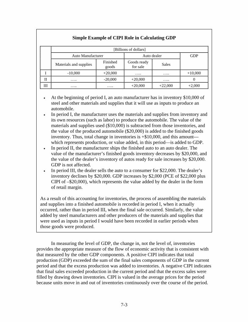
Simple Example of CIPI Role in Calculating GDP
[Billions of dollars]
Auto Manufacturer Auto dealer
Materials and supplies Finished goods
Goods ready for sale Sales
GDP
I -10,000 +20,000 ….. ….. +10,000 II ….. -20,000 +20,000 ….. 0 III ….. ….. +20,000 +22,000 +2,000
• At the beginning of period I, an auto manufacturer has in inventory $10,000 of
steel and other materials and supplies that it will use as inputs to produce an automobile.
• In period I, the manufacturer uses the materials and supplies from inventory and its own resources (such as labor) to produce the automobile. The value of the materials and supplies used ($10,000) is subtracted from those inventories, and the value of the produced automobile ($20,000) is added to the finished goods inventory. Thus, total change in inventories is +$10,000, and this amount—which represents production, or value added, in this period—is added to GDP.
• In period II, the manufacturer ships the finished auto to an auto dealer. The value of the manufacturer’s finished goods inventory decreases by $20,000, and the value of the dealer’s inventory of autos ready for sale increases by $20,000. GDP is not affected.
• In period III, the dealer sells the auto to a consumer for $22,000. The dealer’s inventory declines by $20,000. GDP increases by $2,000 (PCE of $22,000 plus CIPI of –$20,000), which represents the value added by the dealer in the form of retail margin.
As a result of this accounting for inventories, the process of assembling the materials and supplies into a finished automobile is recorded in period I, when it actually occurred, rather than in period III, when the final sale occurred. Similarly, the value added by steel manufacturers and other producers of the materials and supplies that were used as inputs in period I would have been recorded in earlier periods when those goods were produced.
In measuring the level of GDP, the change in, not the level of, inventories provides the appropriate measure of the flow of economic activity that is consistent with that measured by the other GDP components. A positive CIPI indicates that total production (GDP) exceeded the sum of the final sales components of GDP in the current period and that the excess production was added to inventories. A negative CIPI indicates that final sales exceeded production in the current period and that the excess sales were filled by drawing down inventories. CIPI is valued in the average prices for the period because units move in and out of inventories continuously over the course of the period.
7-3
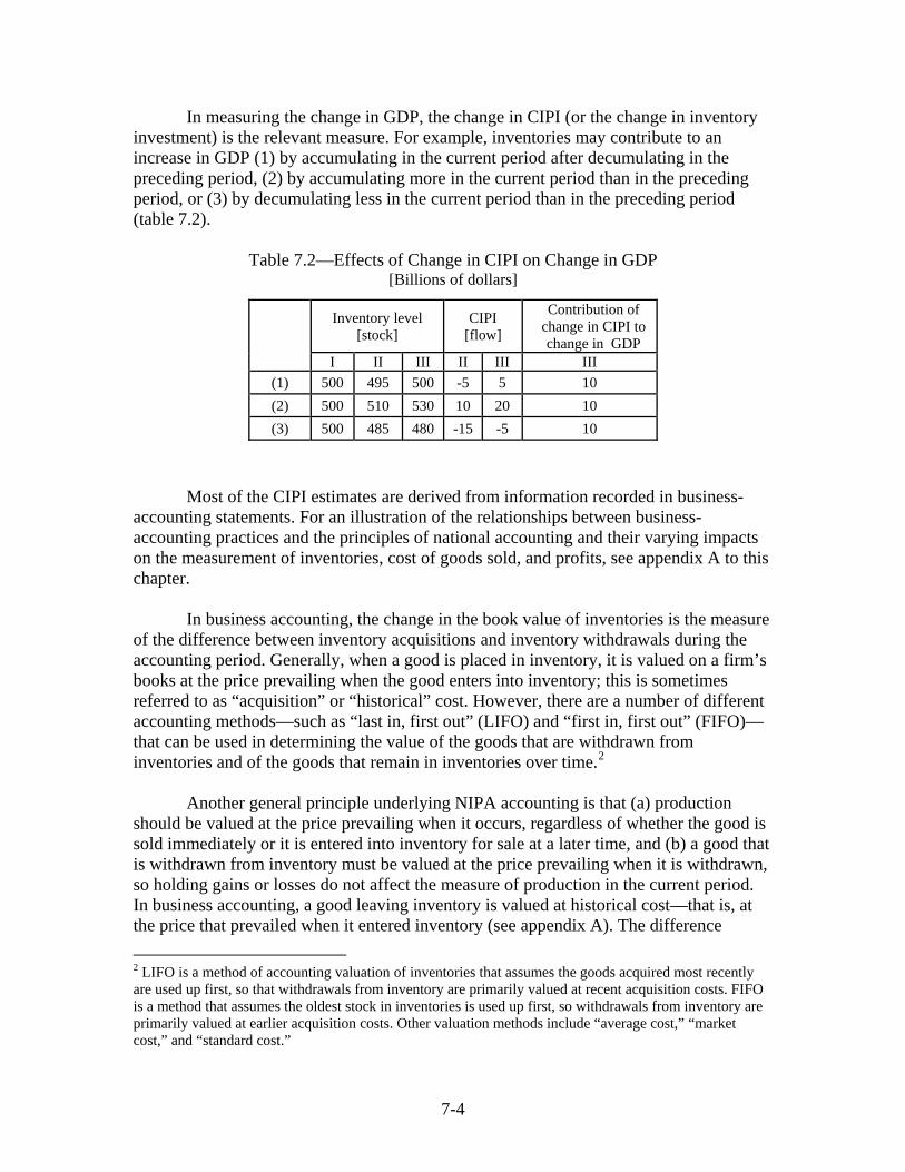
In measuring the change in GDP, the change in CIPI (or the change in inventory investment) is the relevant measure. For example, inventories may contribute to an increase in GDP (1) by accumulating in the current period after decumulating in the preceding period, (2) by accumulating more in the current period than in the preceding period, or (3) by decumulating less in the current period than in the preceding period (table 7.2).
Table 7.2—Effects of Change in CIPI on Change in GDP
[Billions of dollars]
Inventory level [stock]
CIPI [flow]
Contribution of change in CIPI to change in GDP
I II III II III III (1) 500 495 500 -5 5 10 (2) 500 510 530 10 20 10 (3) 500 485 480 -15 -5 10
Most of the CIPI estimates are derived from information recorded in business-accounting statements. For an illustration of the relationships between business-accounting practices and the principles of national accounting and their varying impacts on the measurement of inventories, cost of goods sold, and profits, see appendix A to this chapter.
In business accounting, the change in the book value of inventories is the measure
of the difference between inventory acquisitions and inventory withdrawals during the accounting period. Generally, when a good is placed in inventory, it is valued on a firm’s books at the price prevailing when the good enters into inventory; this is sometimes referred to as “acquisition” or “historical” cost. However, there are a number of different accounting methods—such as “last in, first out” (LIFO) and “first in, first out” (FIFO)—that can be used in determining the value of the goods that are withdrawn from inventories and of the goods that remain in inventories over time.2
Another general principle underlying NIPA accounting is that (a) production
should be valued at the price prevailing when it occurs, regardless of whether the good is sold immediately or it is entered into inventory for sale at a later time, and (b) a good that is withdrawn from inventory must be valued at the price prevailing when it is withdrawn, so holding gains or losses do not affect the measure of production in the current period. In business accounting, a good leaving inventory is valued at historical cost—that is, at the price that prevailed when it entered inventory (see appendix A). The difference 2 LIFO is a method of accounting valuation of inventories that assumes the goods acquired most recently are used up first, so that withdrawals from inventory are primarily valued at recent acquisition costs. FIFO is a method that assumes the oldest stock in inventories is used up first, so withdrawals from inventory are primarily valued at earlier acquisition costs. Other valuation methods include “average cost,” “market cost,” and “standard cost.”
7-4
between the business-accounting measure of change in the book value of inventories and the NIPA measure of CIPI is the gain or loss from holding goods in inventory; it is termed the inventory valuation adjustment (IVA) (see the section “Overview of Source Data and Estimating Methods”).
Recording in the NIPAs As described above, CIPI provides a bridge between final sales in the current period and production in the current period. It is one of the few NIPA components that can be negative. In the seven summary accounts of the NIPAs, CIPI appears in the Domestic Income and Product Account (account 1) as a component of gross private domestic investment and in the Domestic Capital Account (account 6) as a component of gross domestic investment. In the NIPAs, the inventory estimates are generally shown by industry classification, using the North American Industry Classification System, rather than by type of product classification (see chapter 2). Thus, for example, “wholesale trade durable goods inventories” signifies “inventories held by industries engaged in the wholesale trade of durable goods.” CIPI by industry is presented in NIPA table group 5.6. Stocks of private inventories, along with the corresponding aggregate estimates of final sales and inventory-sales ratios, are shown in table group 5.7. The following is a list of the principal NIPA tables that present the inventory estimates: 5.6.5B Change in Private Inventories by Industry 5.6.6B Change in Real Private Inventories by Industry, Chained Dollars 5.7.5B Private Inventories and Domestic Final Sales by Industry 5.7.6B Real Private Inventories and Real Domestic Final Sales by Industry, Chained Dollars 5.7.9B Implicit Price Deflators for Private Inventories by Industry In addition, estimates of change in motor vehicle inventories are shown in tables 7.2.5B and 7.2.6B, and estimates of change in farm inventories are shown in tables 7.3.5 and 7.3.6. BEA also prepares “Underlying Detail” tables for the estimates shown in NIPA table group 5.6, including detail for change in the book values and for IVA by industry, at a greater level of detail than is shown in the published estimates.3 In addition, BEA publishes estimates of real inventories, sales, and inventory-sales ratios for the manufacturing and trade industries each quarter in the Survey of Current Business (generally in the January, April, July, and October issues). BEA also prepares “Underlying Detail” tables for these estimates. 3 Go to www.bea.gov/national/nipa_underlying/Index.asp.
7-5
Overview of Source Data and Estimating Methods
As described earlier in this handbook, the NIPA estimates, including those for CIPI, are prepared using a wide variety of source data (see “Chapter 3: Principal Source Data”) and using estimating methods that adjust the source data to the required NIPA concepts and that fill in gaps in coverage and timing (see chapter 4).
For farm inventories, the estimates of crop and of livestock inventory change are prepared as the product of the change in the physical volume and of the average price, based on data from the U.S. Department of Agriculture (USDA). For example, changes in stocks of wheat on the farm are calculated as wheat harvested and available for sale less wheat sold, valued at average market prices. The estimates of farm inventories include materials and supplies—such as feed, fertilizer, and purchased seed—that are used as inputs to farm production. For crops, the estimates also take into account Commodity Credit Corporation (CCC) loans to producers who use agricultural commodities as collateral.4 Because the estimates of farm inventories are prepared using data on quantities and current prices rather than business-accounting data, an IVA is not calculated.
For nonfarm industries, the estimates of inventory change are generally prepared
by beginning with data on the end-of-period book value of inventories, as reported by private business using a variety of accounting methods.5 The inventory data are then adjusted—annually for 417 detailed industries and monthly for 82 aggregated industries—to value the inventories at a uniform set of prices and to remove holding gains or losses.
More specifically, for manufacturing and trade industries, data on the book value of inventory stocks, inventory turnover, and on the methods of inventory valuation are collected in economic censuses and annual surveys conducted by the Census Bureau. Businesses that use LIFO accounting also provide the Census Bureau with an estimate of the “LIFO reserve,” an adjustment for converting their inventories to a non-LIFO valuation. Data on inventory stocks at the end of the month (and quarter) are collected in the Census Bureau’s monthly surveys. In the Census Bureau’s published reports of manufacturing and trade inventories, all inventories are valued on a “non-LIFO basis.”6
For most other nonfarm industries, annual data on the book value of inventory stocks are available from Internal Revenue Service (IRS) tabulations of business tax
4 Placement of crops as collateral for CCC loans is treated as an addition to farm inventories. Redemption of the crop after loan repayment or forfeiture of the crop after loan default are each treated as a withdrawal from farm inventories. The data on the physical quantities of crops placed, redeemed, and forfeited are from USDA and are valued using average market prices. 5 As a practical matter, the end-of period inventory data reflect losses that result from damage, theft, and other causes, as well as business withdrawals. 6 The Census Bureau reports inventories on a non-LIFO basis because during periods of rising inventories and prices, LIFO accounting may result in stock estimates that are considerably undervalued (see appendix A).
7-6
returns. The data include information on inventory stocks, the proportions of those stocks that are valued on a LIFO basis, and inventory turnover.
For most nonfarm industries, the principal price data used in estimating NIPA
inventories are producer price indexes (PPIs) and import price indexes, both from the Bureau of Labor Statistics (BLS). For the manufacturing and publishing industries, the prices for work-in-process and finished goods inventories consist of a combination of the following: the cost of materials and supplies, based on PPIs; labor costs, based on BEA-constructed unit labor cost indexes; and overhead costs—including rent, depreciation charges, and repair costs—primarily based on PPIs. The BEA labor cost indexes cover compensation of production workers, supervisors, and nonproduction personnel working at the plant and are based on BEA wage data.
At the most detailed level for which BEA prepares estimates, the procedure for nonfarm inventories generally consists of the following steps that yield current-dollar and constant-dollar estimates for CIPI and for the stocks of goods held in inventory. For an illustration of the estimation procedure, see appendix B to this chapter.
1. Separating Census Bureau published inventories (which are on a non-LIFO basis) into those that were reported on a LIFO basis and those that were reported using other accounting methods.
2. Construction of current-period inventory price indexes for each industry, and for manufacturing and for publishing, each stage of fabrication.
3. Construction of monthly cost indexes for each industry, and for manufacturing and publishing, each stage of fabrication.
4. Revaluation of the book-value inventories to yield constant-dollar and current-dollar change in inventories.
5. Calculation of the IVA. 6. Calculation of current-dollar and constant-dollar stocks.
As noted earlier, the IVA is the measure of the holding gains or losses that are removed from the business-accounting measure of inventory change. It is calculated for all inventory-accounting methods, regardless of whether inventories are accumulating or decumulating over the recording period. However, under LIFO accounting, if inventories are accumulating, withdrawals are already valued at current-period prices; thus, CIPI and change in the book value are equal, and the IVA is zero (see appendix A).
In the NIPAs, the IVA is also shown on the income side of the accounts in order to exclude the inventory holding gains (or losses) from business income in the calculation of corporate profits and of nonfarm proprietors’ income.7 Since profit and income data come from IRS tabulations, the product-side IVA must be adjusted for any accounting-basis differences between the IRS data and the Census Bureau data. (The estimates for nonfarm industries other than manufacturing and trade are already based on IRS data, so in most cases no adjustment is needed for those industries.) 7 See NIPA table 6.14D, “Inventory Valuation Adjustment to Nonfarm Incomes by Legal Form of Organization and by Industry.”
7-7
In estimating the stocks of private inventories, the constant-dollar estimates are
derived first, using the perpetual inventory method—that is, by adding the change in real private inventories during the period to the real stocks at the end of the preceding period (see “perpetual inventory method” in “Chapter 4: Estimating Methods”). The end-of-period current-dollar estimates of the stock of private inventories are then derived by “reflation”—that is, by multiplying estimates of the end-of-period real-stocks by appropriate price indexes.
Table 7.A at the end of this chapter summarizes the source data and estimating methods that are used to prepare the benchmark-year, nonbenchmark-year, current quarterly, and quantity (inflation-adjusted) estimates for the CIPI categories that are shown by industry in NIPA table group 5.6. Benchmark-year estimates
For manufacturing, data on the book value of inventory stocks and on the methods
of inventory valuation are available from the Census Bureau’s economic census. Manufacturing establishments report their end-of-year inventory levels and their inventories by stage of fabrication (finished, work-in-process, and materials and supplies). Information on the distribution of costs in the manufacturing sector among materials, labor, and overhead is used in the calculation of cost of goods sold and of inventory turnover ratios (see appendix B). The commodity composition of materials held in inventory is assumed to be the same as that for materials purchased by the industry, which, in turn, is derived from BEA’s benchmark input-output accounts, based on information from the economic censuses on materials “consumed” by industry. This information is used in the calculation of materials held in inventory.
For wholesale trade, data on the book value of inventory stocks are available from
the annual wholesale trade survey and data on the methods of inventory valuation are available from the economic census. For retail trade, the data on the book value of inventory stocks and on inventory valuation are available from the annual retail trade survey. Retail and wholesale trade establishments report their inventories of goods for sale at the end of the year.8 LIFO users also report the LIFO reserve and the LIFO value after adjustment for the reserve. For wholesale and retail trade, data on purchases from the annual surveys are used in the calculation of cost of goods sold and of inventory-turnover ratios. In addition, data on product-line sales by industry are used in the calculation of commodities held in inventory.
For the mining and construction industries, the inventory estimates for benchmark
years are based on information from the economic census. For the publishing industry, the inventory estimates are based on information from the services annual survey. For all 8 The inventory data published by the Census Bureau include inventories that are owned by U.S. establishments but are held abroad. BEA adjusts these data in order to exclude those inventories.
7-8

other nonfarm industries, the estimates for all years except the most recent year are based on IRS tabulations of income tax returns for corporations and for sole proprietorships and partnerships.
For farm inventories, the estimates for all years (benchmark and nonbenchmark)
are based on USDA annual reports. Annual changes in farm inventories of crops are estimated as crops harvested in the period and available for sale (that is, not including crops retained for personal consumption) less crops sold in the period plus net CCC loan transactions. The annual quantity changes for each crop are valued at average market prices received by farmers during the calendar year. Annual changes in farm inventories of livestock are estimated from USDA surveys of inventory stocks on farms. For each livestock commodity, annual quantity changes are valued at average market price per head. Nonbenchmark-year estimates
For years other than benchmark years and the most recent year, the inventory
estimates for the manufacturing, trade, and publishing industries are primarily based on the Census Bureau’s annual survey of manufactures, annual wholesale trade survey, annual retail trade survey, and service annual survey. Respondents to these surveys report LIFO, LIFO reserve, and non-LIFO valuations separately. In addition, respondents in the manufacturing sector report information on the distribution of costs among materials, labor, and overhead and those in retail and wholesale report purchases; this information is used in the calculation of cost of goods sold and of inventory-turnover ratios.
For the mining, utilities, and construction industries, as well as for other nonfarm
industries, the estimates for all nonbenchmark years except the most recent year are based on IRS tabulations of income tax returns for corporations and for sole proprietorships and partnerships.
The sources and methods for deriving the nonbenchmark-year estimates of farm
inventories are the same as those for the benchmark estimates (see above).
Most-recent-year and current-quarterly estimates The inventory estimates for the most recent year and for the current quarters for
the manufacturing and trade industries (except those for retail auto dealers) are based on the following Census Bureau surveys: monthly survey of manufacturers’ shipments, inventories, and orders; monthly wholesale trade survey; and monthly retail trade and food services survey. The data for manufacturing, wholesale trade, and retail trade are summarized in the Census Bureau’s monthly “Business Sales and Inventories” release. The quarterly estimates for the manufacturing and trade industries are calculated as end-of-month inventories for the final month of the quarter less end-of-month inventories for the final month of the preceding quarter.
7-9
For retail auto dealers, inventory estimates for the most recent year and for the
current quarters are primarily based on a reconciliation with BEA’s unit-based estimates, which are based on the monthly unit data from Wards’ Automotive Reports and on average price data from J.D. Power and Associates.
For utilities, the quantity estimates are prepared first, using data on changes in the
physical stocks of coal, petroleum, and natural gas and on base-year prices from the Energy Information Administration. The current-dollar estimates are then derived by “reflation”—that is, by multiplying the quantity estimates by appropriate price data from the Bureau of Labor Statistics (BLS).
For all other nonfarm industries, estimates for the most recent year and for the
current quarters are prepared by starting with the previous annual level and by assuming that inventories move proportionately with certain other indicator series chosen for each industry or by judgmental trend. The indicator series include inventory information from the Census Bureau’s quarterly financial reports and monthly measures of activity from the Census Bureau’s construction statistics and from BLS industry wage data.
For farm inventories, quarterly estimates of crop inventories, which are calculated
only for total crops, are based on a BEA quarterly allocation of USDA annual projections of crop output and cash receipts. Quarterly estimates of livestock inventories are based on USDA data by type of livestock.
Quantity and price estimates The quantity estimates for the detailed inventory components are primarily derived by deflation, as shown in appendix B. (For a general description of the deflation method, see “Estimates for detailed components” in chapter 4.) In the NIPAs, the aggregate measures for most of the components of real GDP are calculated from the detailed components as chain-type quantity and price indexes (see “Estimates for NIPA aggregates” in chapter 4). However, the detailed CIPI estimates may contain negative values (which could require the Fisher formula to take the square root of a negative number).9 Therefore, the end-of period, chain-weighted estimates of inventory stocks are calculated first, and the CIPI chained-dollar estimates are then calculated as the differences between these estimates. Under this procedure, inventory stocks are used as weights for inventory flows, though the composition of the stocks may differ from the composition of the inventory investment flows.
9 The inability to calculate Fisher quantity indexes for CIPI does not extend to higher level aggregates (such as gross private domestic investment and GDP) that include CIPI as a component, because the negative values of CIPI are small relative to the levels of the other components of those aggregates.
7-10
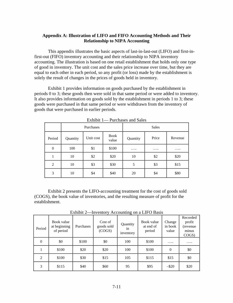
Appendix A: Illustration of LIFO and FIFO Accounting Methods and Their
Relationship to NIPA Accounting This appendix illustrates the basic aspects of last-in-last-out (LIFO) and first-in-first-out (FIFO) inventory accounting and their relationship to NIPA inventory accounting. The illustration is based on one retail establishment that holds only one type of good in inventory. The unit cost and the sales price increase over time, but they are equal to each other in each period, so any profit (or loss) made by the establishment is solely the result of changes in the prices of goods held in inventory.
Exhibit 1 provides information on goods purchased by the establishment in periods 0 to 3; these goods then were sold in that same period or were added to inventory. It also provides information on goods sold by the establishment in periods 1 to 3; these goods were purchased in that same period or were withdrawn from the inventory of goods that were purchased in earlier periods.
Exhibit 1— Purchases and Sales Purchases Sales
Period
Quantity Unit cost Book
value
Quantity Price Revenue
0 100 $1 $100 ….. ….. …..
1 10 $2 $20 10 $2 $20
2 10 $3 $30 5 $3 $15
3 10 $4 $40 20 $4 $80
Exhibit 2 presents the LIFO-accounting treatment for the cost of goods sold (COGS), the book value of inventories, and the resulting measure of profit for the establishment.
Exhibit 2—Inventory Accounting on a LIFO Basis
Period
Book value at beginning
of period Purchases
Cost of goods sold (COGS)
Quantity
in inventory
Book value at end of period
Change in book value
Recorded profit
(revenue minus
COGS)
0 $0 $100 $0 100 $100 ….. …..
1 $100 $20 $20 100 $100 0 $0
2 $100 $30 $15 105 $115 $15 $0
3 $115 $40 $60 95 $95 –$20 $20
7-11
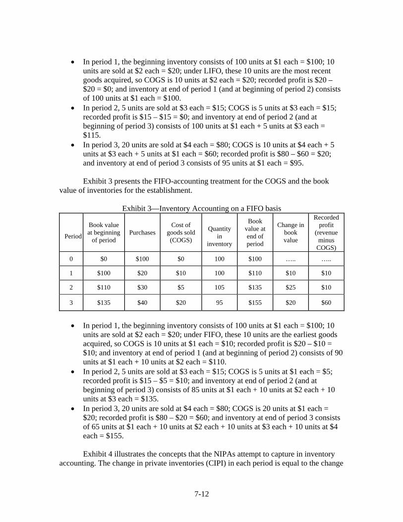
• In period 1, the beginning inventory consists of 100 units at $1 each = $100; 10
units are sold at $2 each = $20; under LIFO, these 10 units are the most recent goods acquired, so COGS is 10 units at $2 each = $20; recorded profit is $20 – $20 = $0; and inventory at end of period 1 (and at beginning of period 2) consists of 100 units at $1 each = $100.
• In period 2, 5 units are sold at $3 each = $15; COGS is 5 units at $3 each = $15; recorded profit is $15 – $15 = $0; and inventory at end of period 2 (and at beginning of period 3) consists of 100 units at $1 each + 5 units at $3 each = $115.
• In period 3, 20 units are sold at $4 each = $80; COGS is 10 units at $4 each + 5 units at $3 each + 5 units at $1 each = $60; recorded profit is $80 – $60 = $20; and inventory at end of period 3 consists of 95 units at $1 each = $95.
Exhibit 3 presents the FIFO-accounting treatment for the COGS and the book value of inventories for the establishment.
Exhibit 3—Inventory Accounting on a FIFO basis
Period
Book value at beginning
of period Purchases
Cost of goods sold (COGS)
Quantity
in inventory
Book value at end of period
Change in book value
Recorded profit
(revenue minus
COGS)
0 $0 $100 $0 100 $100 ….. …..
1 $100 $20 $10 100 $110 $10 $10
2 $110 $30 $5 105 $135 $25 $10
3 $135 $40 $20 95 $155 $20 $60
• In period 1, the beginning inventory consists of 100 units at $1 each = $100; 10
units are sold at $2 each = $20; under FIFO, these 10 units are the earliest goods acquired, so COGS is 10 units at $1 each = $10; recorded profit is $20 – $10 = $10; and inventory at end of period 1 (and at beginning of period 2) consists of 90 units at $1 each + 10 units at $2 each = $110.
• In period 2, 5 units are sold at $3 each = $15; COGS is 5 units at $1 each = $5; recorded profit is $15 – $5 = $10; and inventory at end of period 2 (and at beginning of period 3) consists of 85 units at $1 each + 10 units at $2 each + 10 units at $3 each = $135.
• In period 3, 20 units are sold at $4 each = $80; COGS is 20 units at $1 each = $20; recorded profit is $80 – $20 = $60; and inventory at end of period 3 consists of 65 units at $1 each + 10 units at $2 each + 10 units at $3 each + 10 units at $4 each = $155.
Exhibit 4 illustrates the concepts that the NIPAs attempt to capture in inventory
accounting. The change in private inventories (CIPI) in each period is equal to the change
7-12
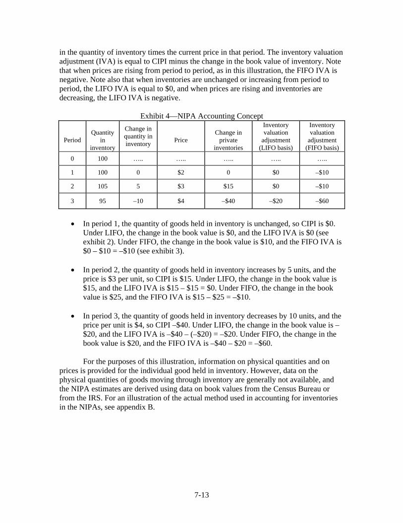
in the quantity of inventory times the current price in that period. The inventory valuation adjustment (IVA) is equal to CIPI minus the change in the book value of inventory. Note that when prices are rising from period to period, as in this illustration, the FIFO IVA is negative. Note also that when inventories are unchanged or increasing from period to period, the LIFO IVA is equal to $0, and when prices are rising and inventories are decreasing, the LIFO IVA is negative.
Exhibit 4—NIPA Accounting Concept
Period
Quantity
in inventory
Change in quantity in inventory
Price
Change in
private inventories
Inventory valuation
adjustment (LIFO basis)
Inventory valuation
adjustment (FIFO basis)
0 100 ….. ….. ….. ….. …..
1 100 0 $2 0 $0 –$10
2 105 5 $3 $15 $0 –$10
3 95 –10 $4 –$40 –$20 –$60
• In period 1, the quantity of goods held in inventory is unchanged, so CIPI is $0.
Under LIFO, the change in the book value is $0, and the LIFO IVA is $0 (see exhibit 2). Under FIFO, the change in the book value is $10, and the FIFO IVA is $0 – $10 = –$10 (see exhibit 3).
• In period 2, the quantity of goods held in inventory increases by 5 units, and the price is $3 per unit, so CIPI is $15. Under LIFO, the change in the book value is $15, and the LIFO IVA is $15 – $15 = $0. Under FIFO, the change in the book value is $25, and the FIFO IVA is $15 – $25 = –$10.
• In period 3, the quantity of goods held in inventory decreases by 10 units, and the price per unit is $4, so CIPI –$40. Under LIFO, the change in the book value is –$20, and the LIFO IVA is –$40 – (–$20) = –$20. Under FIFO, the change in the book value is $20, and the FIFO IVA is –$40 – $20 = –$60.
For the purposes of this illustration, information on physical quantities and on
prices is provided for the individual good held in inventory. However, data on the physical quantities of goods moving through inventory are generally not available, and the NIPA estimates are derived using data on book values from the Census Bureau or from the IRS. For an illustration of the actual method used in accounting for inventories in the NIPAs, see appendix B.
7-13
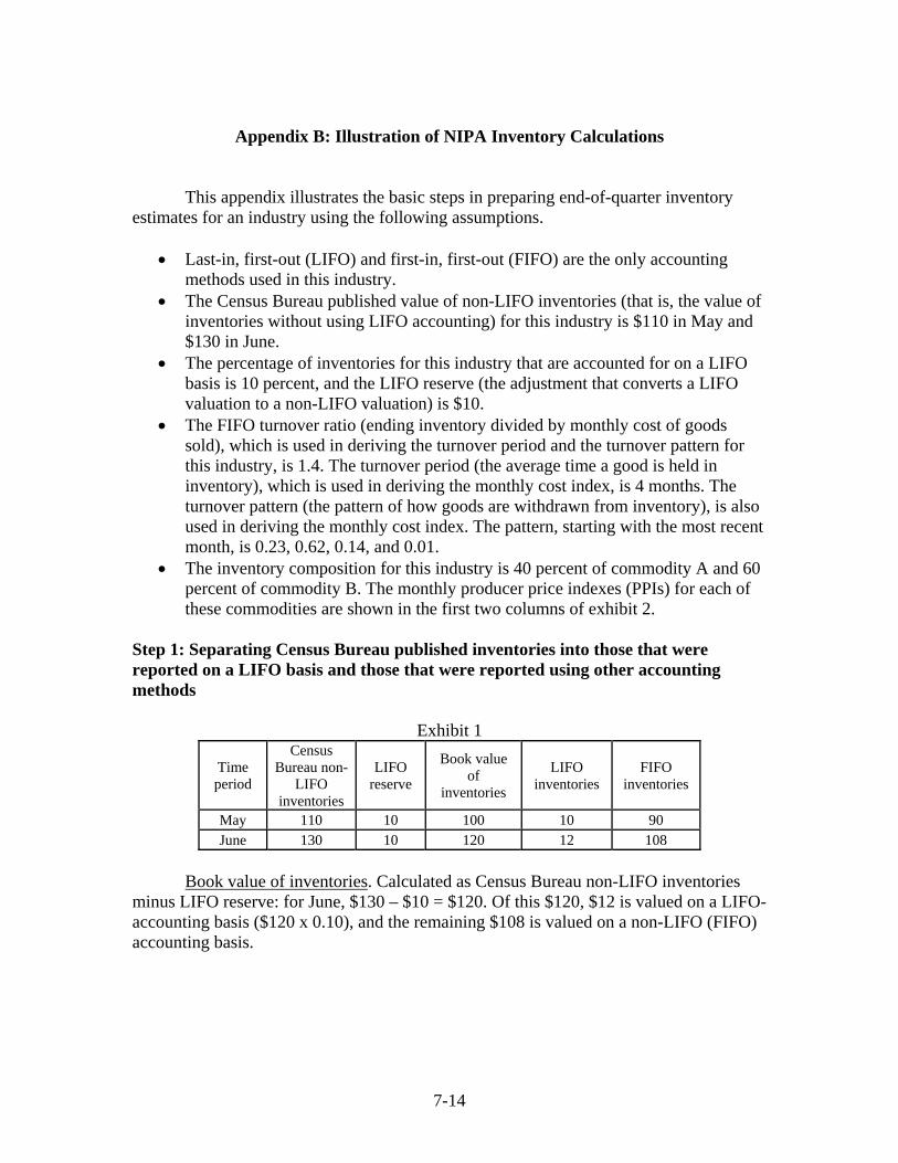
Appendix B: Illustration of NIPA Inventory Calculations
This appendix illustrates the basic steps in preparing end-of-quarter inventory
estimates for an industry using the following assumptions.
• Last-in, first-out (LIFO) and first-in, first-out (FIFO) are the only accounting methods used in this industry.
• The Census Bureau published value of non-LIFO inventories (that is, the value of inventories without using LIFO accounting) for this industry is $110 in May and $130 in June.
• The percentage of inventories for this industry that are accounted for on a LIFO basis is 10 percent, and the LIFO reserve (the adjustment that converts a LIFO valuation to a non-LIFO valuation) is $10.
• The FIFO turnover ratio (ending inventory divided by monthly cost of goods sold), which is used in deriving the turnover period and the turnover pattern for this industry, is 1.4. The turnover period (the average time a good is held in inventory), which is used in deriving the monthly cost index, is 4 months. The turnover pattern (the pattern of how goods are withdrawn from inventory), is also used in deriving the monthly cost index. The pattern, starting with the most recent month, is 0.23, 0.62, 0.14, and 0.01.
• The inventory composition for this industry is 40 percent of commodity A and 60 percent of commodity B. The monthly producer price indexes (PPIs) for each of these commodities are shown in the first two columns of exhibit 2.
Step 1: Separating Census Bureau published inventories into those that were reported on a LIFO basis and those that were reported using other accounting methods
Exhibit 1
Time period
Census Bureau non-
LIFO inventories
LIFO reserve
Book value of
inventories
LIFO inventories
FIFO inventories
May 110 10 100 10 90 June 130 10 120 12 108
Book value of inventories. Calculated as Census Bureau non-LIFO inventories minus LIFO reserve: for June, $130 – $10 = $120. Of this $120, $12 is valued on a LIFO-accounting basis ($120 x 0.10), and the remaining $108 is valued on a non-LIFO (FIFO) accounting basis.
7-14
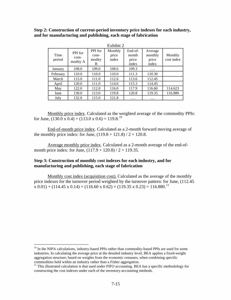
Step 2: Construction of current-period inventory price indexes for each industry, and for manufacturing and publishing, each stage of fabrication
Exhibit 2
Time period
PPI for com-
modity A
PPI for com-
modity B
Monthly price index
End-of- month price index
Average monthly
price index
Monthly cost index
January 108.0 109.0 108.6 109.3 …. February 110.0 110.0 110.0 111.3 110.30 March 115.0 111.0 112.6 113.6 112.45 April 120.0 111.0 114.6 115.3 114.45 May 122.0 112.0 116.0 117.9 116.60 114.623 June 130.0 113.0 119.8 120.8 119.35 116.880 July 132.0 115.0 121.8 …. ….
Monthly price index. Calculated as the weighted average of the commodity PPIs:
for June, (130.0 x 0.4) + (113.0 x 0.6) = 119.8.10 End-of-month price index. Calculated as a 2-month forward moving average of
the monthly price index: for June, (119.8 + 121.8) / 2 = 120.8. Average monthly price index. Calculated as a 2-month average of the end-of-
month price index: for June, (117.9 + 120.8) / 2 = 119.35.
Step 3: Construction of monthly cost indexes for each industry, and for manufacturing and publishing, each stage of fabrication
Monthly cost index (acquisition cost). Calculated as the average of the monthly
price indexes for the turnover period weighted by the turnover pattern: for June, (112.45 x 0.01) + (114.45 x 0.14) + (116.60 x 0.62) + (119.35 x 0.23) = 116.880.11
10 In the NIPA calculations, industry-based PPIs rather than commodity-based PPIs are used for some industries. In calculating the average price at the detailed industry level, BEA applies a fixed-weight aggregation structure, based on weights from the economic censuses, when combining specific commodities held within an industry rather than a Fisher aggregation. 11 This illustrated calculation is that used under FIFO accounting. BEA has a specific methodology for constructing the cost indexes under each of the inventory-accounting methods.
7-15
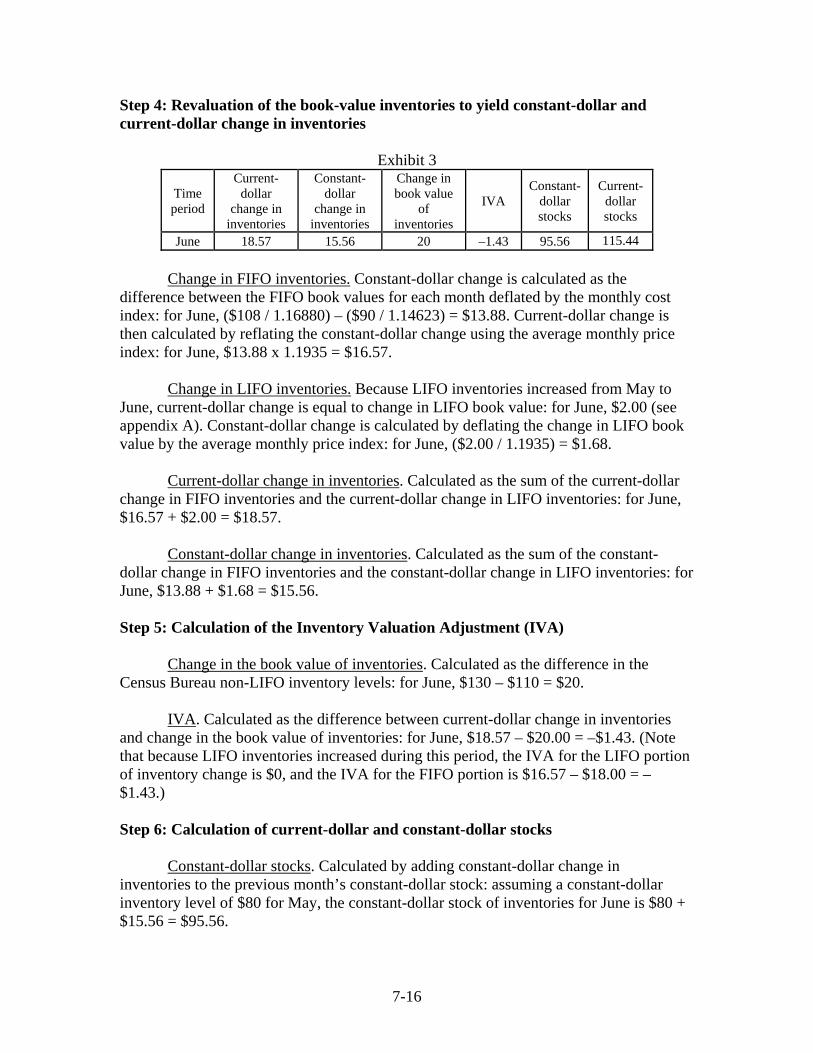
Step 4: Revaluation of the book-value inventories to yield constant-dollar and current-dollar change in inventories
Exhibit 3
Time period
Current-dollar
change in inventories
Constant-dollar
change in inventories
Change in book value
of inventories
IVA Constant-
dollar stocks
Current-dollar stocks
June 18.57 15.56 20 –1.43 95.56 115.44 Change in FIFO inventories. Constant-dollar change is calculated as the difference between the FIFO book values for each month deflated by the monthly cost index: for June, ($108 / 1.16880) – ($90 / 1.14623) = $13.88. Current-dollar change is then calculated by reflating the constant-dollar change using the average monthly price index: for June, $13.88 x 1.1935 = $16.57. Change in LIFO inventories. Because LIFO inventories increased from May to June, current-dollar change is equal to change in LIFO book value: for June, $2.00 (see appendix A). Constant-dollar change is calculated by deflating the change in LIFO book value by the average monthly price index: for June, ($2.00 / 1.1935) = $1.68. Current-dollar change in inventories. Calculated as the sum of the current-dollar change in FIFO inventories and the current-dollar change in LIFO inventories: for June, $16.57 + $2.00 = $18.57. Constant-dollar change in inventories. Calculated as the sum of the constant-dollar change in FIFO inventories and the constant-dollar change in LIFO inventories: for June, $13.88 + $1.68 = $15.56. Step 5: Calculation of the Inventory Valuation Adjustment (IVA) Change in the book value of inventories. Calculated as the difference in the Census Bureau non-LIFO inventory levels: for June, $130 – $110 = $20. IVA. Calculated as the difference between current-dollar change in inventories and change in the book value of inventories: for June, $18.57 – $20.00 = –$1.43. (Note that because LIFO inventories increased during this period, the IVA for the LIFO portion of inventory change is $0, and the IVA for the FIFO portion is $16.57 – $18.00 = –$1.43.) Step 6: Calculation of current-dollar and constant-dollar stocks Constant-dollar stocks. Calculated by adding constant-dollar change in inventories to the previous month’s constant-dollar stock: assuming a constant-dollar inventory level of $80 for May, the constant-dollar stock of inventories for June is $80 + $15.56 = $95.56.
7-16
7-17
Current-dollar stocks. Calculated by reflating constant-dollar stocks using end-of-month prices: for June, $95.56 x 1.208 = $115.44. Note that while the difference between the constant-dollar stocks for May and June ($15.56) is equal to constant-dollar CIPI,12 the difference between the current-dollar stocks for May and June ($19.88) is not equal to current-dollar CIPI ($18.57). This is because the current-dollar stocks are valued at end-of-period prices, while CIPI is valued using average prices for the period.
12 Because quarterly and monthly estimates in the NIPAs are expressed at annual rates, it is necessary to divide the CIPI estimates by 4 and by 12, respectively, to observe the equality.
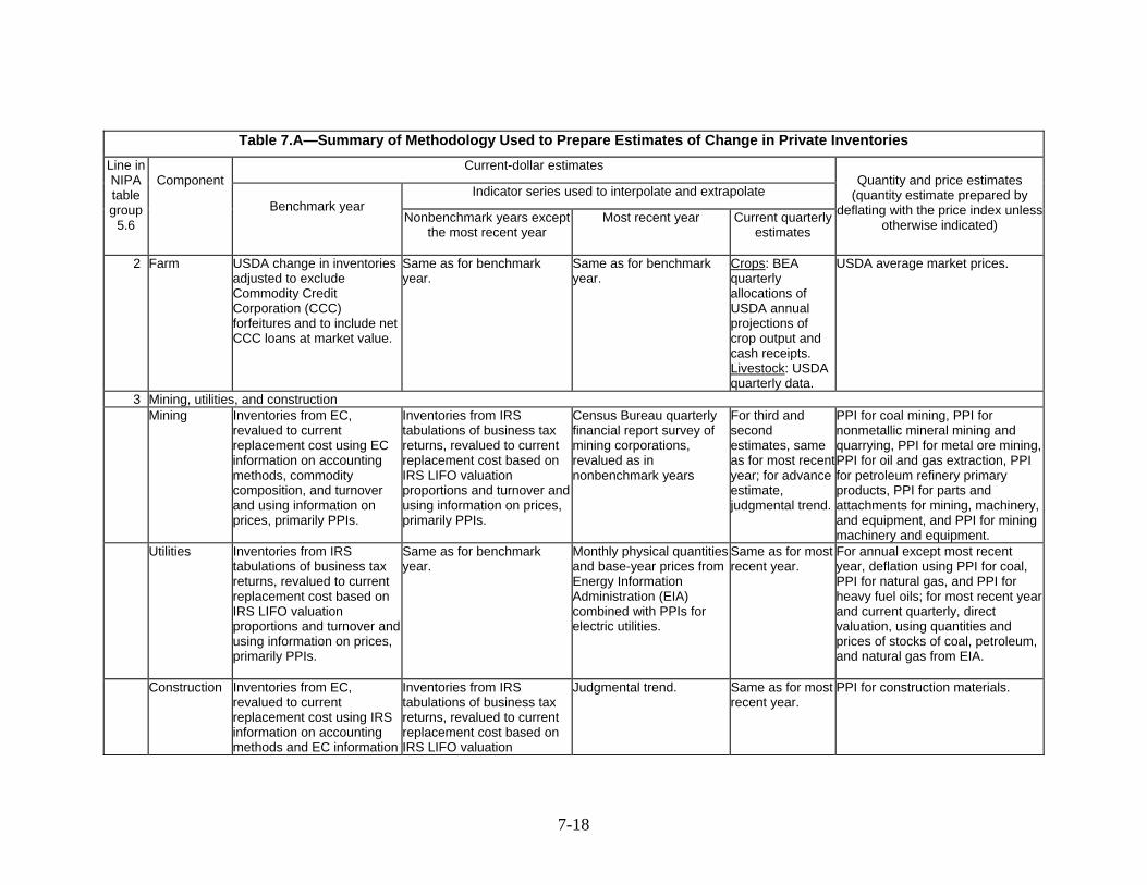
Table 7.A—Summary of Methodology Used to Prepare Estimates of Change in Private Inventories Current-dollar estimates
Indicator series used to interpolate and extrapolate
Line in NIPA table group
5.6
Component
Benchmark year
Nonbenchmark years except the most recent year
Most recent year
Current quarterly estimates
Quantity and price estimates
(quantity estimate prepared by deflating with the price index unless
otherwise indicated)
2 Farm USDA change in inventories adjusted to exclude Commodity Credit Corporation (CCC) forfeitures and to include net CCC loans at market value.
Same as for benchmark year.
Same as for benchmark year.
Crops: BEA quarterly allocations of USDA annual projections of crop output and cash receipts. Livestock: USDA quarterly data.
USDA average market prices.
3 Mining, utilities, and construction Mining Inventories from EC,
revalued to current replacement cost using EC information on accounting methods, commodity composition, and turnover and using information on prices, primarily PPIs.
Inventories from IRS tabulations of business tax returns, revalued to current replacement cost based on IRS LIFO valuation proportions and turnover andusing information on prices, primarily PPIs.
Census Bureau quarterly financial report survey of mining corporations, revalued as in nonbenchmark years
For third and second estimates, same as for most recent year; for advance estimate, judgmental trend.
PPI for coal mining, PPI for nonmetallic mineral mining and quarrying, PPI for metal ore mining, PPI for oil and gas extraction, PPI for petroleum refinery primary products, PPI for parts and attachments for mining, machinery, and equipment, and PPI for mining machinery and equipment.
Utilities Inventories from IRS tabulations of business tax returns, revalued to current replacement cost based on IRS LIFO valuation proportions and turnover and using information on prices, primarily PPIs.
Same as for benchmark year.
Monthly physical quantitiesand base-year prices from Energy Information Administration (EIA) combined with PPIs for electric utilities.
Same as for most recent year.
For annual except most recent year, deflation using PPI for coal, PPI for natural gas, and PPI for heavy fuel oils; for most recent year and current quarterly, direct valuation, using quantities and prices of stocks of coal, petroleum, and natural gas from EIA.
Construction Inventories from EC, revalued to current replacement cost using IRS information on accounting methods and EC information
Inventories from IRS tabulations of business tax returns, revalued to current replacement cost based on IRS LIFO valuation
Judgmental trend. Same as for most recent year.
PPI for construction materials.
7-18
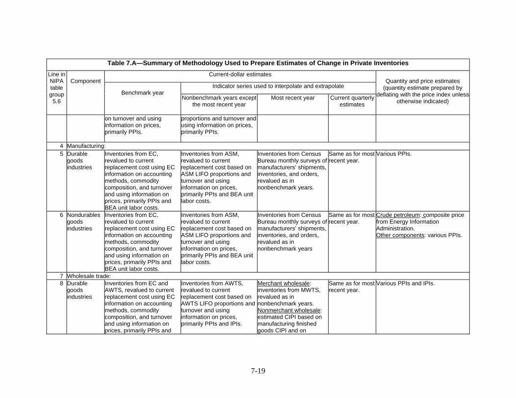
Table 7.A—Summary of Methodology Used to Prepare Estimates of Change in Private Inventories Current-dollar estimates
Indicator series used to interpolate and extrapolate
Line in NIPA table group
5.6
Component
Benchmark year
Nonbenchmark years except the most recent year
Most recent year
Current quarterly estimates
Quantity and price estimates
(quantity estimate prepared by deflating with the price index unless
otherwise indicated)
on turnover and using information on prices, primarily PPIs.
proportions and turnover and using information on prices, primarily PPIs.
4 Manufacturing: 5 Durable
goods industries
Inventories from EC, revalued to current replacement cost using EC information on accounting methods, commodity composition, and turnover and using information on prices, primarily PPIs and BEA unit labor costs.
Inventories from ASM, revalued to current replacement cost based on ASM LIFO proportions and turnover and using information on prices, primarily PPIs and BEA unit labor costs.
Inventories from Census Bureau monthly surveys of manufacturers’ shipments, inventories, and orders, revalued as in nonbenchmark years.
Same as for most recent year.
Various PPIs.
6 Nondurables goods industries
Inventories from EC, revalued to current replacement cost using EC information on accounting methods, commodity composition, and turnover and using information on prices, primarily PPIs and BEA unit labor costs.
Inventories from ASM, revalued to current replacement cost based on ASM LIFO proportions and turnover and using information on prices, primarily PPIs and BEA unit labor costs.
Inventories from Census Bureau monthly surveys of manufacturers’ shipments, inventories, and orders, revalued as in nonbenchmark years
Same as for most recent year.
Crude petroleum: composite price from Energy Information Administration. Other components: various PPIs.
7 Wholesale trade: 8 Durable
goods industries
Inventories from EC and AWTS, revalued to current replacement cost using EC information on accounting methods, commodity composition, and turnover and using information on prices, primarily PPIs and
Inventories from AWTS, revalued to current replacement cost based on AWTS LIFO proportions and turnover and using information on prices, primarily PPIs and IPIs.
Merchant wholesale: inventories from MWTS, revalued as in nonbenchmark years. Nonmerchant wholesale: estimated CIPI based on manufacturing finished goods CIPI and on
Same as for most recent year.
Various PPIs and IPIs.
7-19
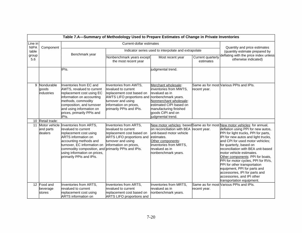
Table 7.A—Summary of Methodology Used to Prepare Estimates of Change in Private Inventories Current-dollar estimates
Indicator series used to interpolate and extrapolate
Line in NIPA table group
5.6
Component
Benchmark year
Nonbenchmark years except the most recent year
Most recent year
Current quarterly estimates
Quantity and price estimates
(quantity estimate prepared by deflating with the price index unless
otherwise indicated)
IPIs. judgmental trend.
9 Nondurable goods industries
Inventories from EC and AWTS, revalued to current replacement cost using EC information on accounting methods, commodity composition, and turnover and using information on prices, primarily PPIs and IPIs.
Inventories from AWTS, revalued to current replacement cost based on AWTS LIFO proportions and turnover and using information on prices, primarily PPIs and IPIs.
Merchant wholesale: inventories from MWTS, revalued as in nonbenchmark years. Nonmerchant wholesale: estimated CIPI based on manufacturing finished goods CIPI and on judgmental trend.
Same as for most recent year.
Various PPIs and IPIs.
10 Retail trade: 11 Motor vehicle
and parts dealers
Inventories from ARTS, revalued to current replacement cost using ARTS information on accounting methods and turnover, EC information on commodity composition, andusing information on prices, primarily PPIs and IPIs.
Inventories from ARTS, revalued to current replacement cost based on ARTS LIFO proportions and turnover and using information on prices, primarily PPIs and IPIs.
New motor vehicles: based on reconciliation with BEA unit-based motor vehicle estimates. Other components: inventories from MRTS, revalued as in nonbenchmark years.
Same as for most recent year.
New motor vehicles: for annual, deflation using PPI for new autos, PPI for light trucks, PPI for parts, IPI for new autos and light trucks, and CPI for used motor vehicles; for quarterly, based on reconciliation with BEA unit-based motor vehicle estimates. Other components: PPI for boats, PPI for motor cycles, PPI for RVs, PPI for other transportation equipment, PPI for parts and accessories, IPI for parts and accessories, and IPI other transportation equipment.
12 Food and beverage stores
Inventories from ARTS, revalued to current replacement cost using ARTS information on
Inventories from ARTS, revalued to current replacement cost based on ARTS LIFO proportions and
Inventories from MRTS, revalued as in nonbenchmark years.
Same as for most recent year.
Various PPIs and IPIs.
7-20
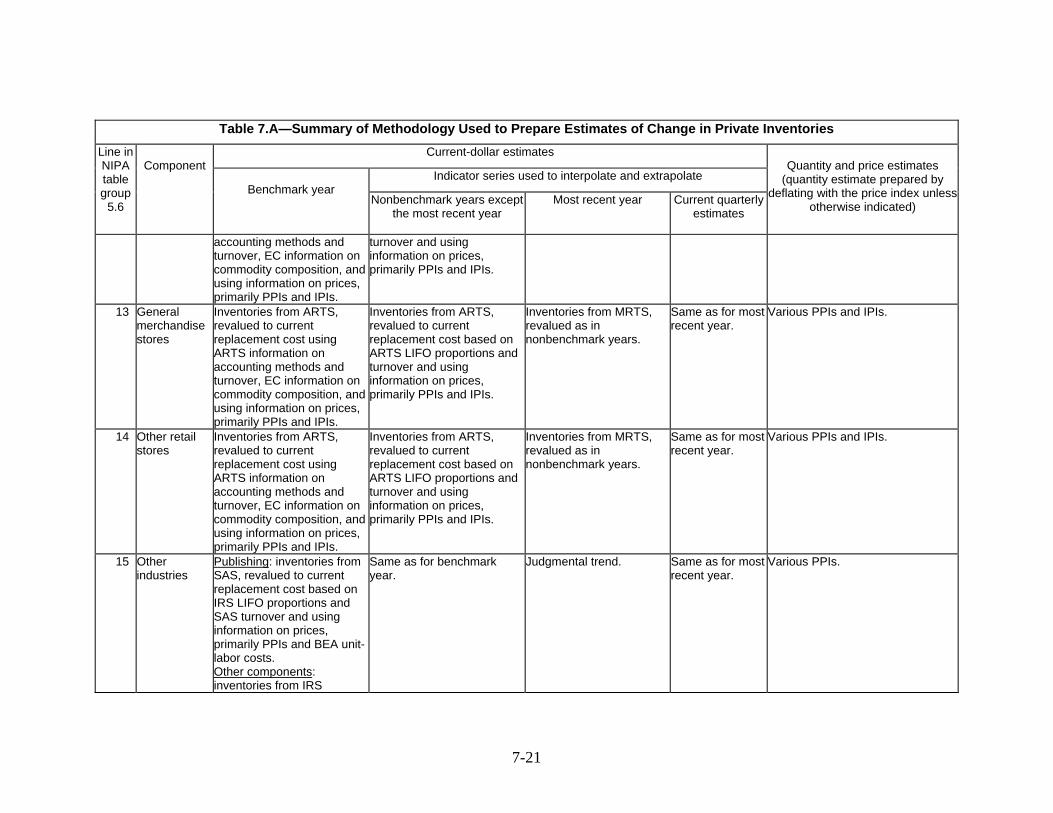
Table 7.A—Summary of Methodology Used to Prepare Estimates of Change in Private Inventories Current-dollar estimates
Indicator series used to interpolate and extrapolate
Line in NIPA table group
5.6
Component
Benchmark year
Nonbenchmark years except the most recent year
Most recent year
Current quarterly estimates
Quantity and price estimates
(quantity estimate prepared by deflating with the price index unless
otherwise indicated)
accounting methods and turnover, EC information on commodity composition, andusing information on prices, primarily PPIs and IPIs.
turnover and using information on prices, primarily PPIs and IPIs.
13 General merchandise stores
Inventories from ARTS, revalued to current replacement cost using ARTS information on accounting methods and turnover, EC information on commodity composition, and using information on prices, primarily PPIs and IPIs.
Inventories from ARTS, revalued to current replacement cost based on ARTS LIFO proportions and turnover and using information on prices, primarily PPIs and IPIs.
Inventories from MRTS, revalued as in nonbenchmark years.
Same as for most recent year.
Various PPIs and IPIs.
14 Other retail stores
Inventories from ARTS, revalued to current replacement cost using ARTS information on accounting methods and turnover, EC information on commodity composition, andusing information on prices, primarily PPIs and IPIs.
Inventories from ARTS, revalued to current replacement cost based on ARTS LIFO proportions and turnover and using information on prices, primarily PPIs and IPIs.
Inventories from MRTS, revalued as in nonbenchmark years.
Same as for most recent year.
Various PPIs and IPIs.
15 Other industries
Publishing: inventories from SAS, revalued to current replacement cost based on IRS LIFO proportions and SAS turnover and using information on prices, primarily PPIs and BEA unit-labor costs. Other components: inventories from IRS
Same as for benchmark year.
Judgmental trend. Same as for most recent year.
Various PPIs.
7-21
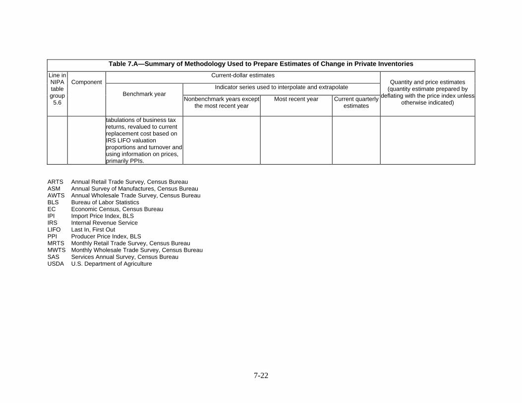
7-22
Table 7.A—Summary of Methodology Used to Prepare Estimates of Change in Private Inventories Current-dollar estimates
Indicator series used to interpolate and extrapolate
Line in NIPA table group
5.6
Component
Benchmark year
Nonbenchmark years except the most recent year
Most recent year
Current quarterly estimates
Quantity and price estimates
(quantity estimate prepared by deflating with the price index unless
otherwise indicated)
tabulations of business tax returns, revalued to current replacement cost based on IRS LIFO valuation proportions and turnover and using information on prices, primarily PPIs.
ARTS Annual Retail Trade Survey, Census Bureau ASM Annual Survey of Manufactures, Census Bureau AWTS Annual Wholesale Trade Survey, Census Bureau BLS Bureau of Labor Statistics EC Economic Census, Census Bureau IPI Import Price Index, BLS IRS Internal Revenue Service LIFO Last In, First Out PPI Producer Price Index, BLS MRTS Monthly Retail Trade Survey, Census Bureau MWTS Monthly Wholesale Trade Survey, Census Bureau SAS Services Annual Survey, Census Bureau USDA U.S. Department of Agriculture