conceptual design for a re-entrant type fuel channel for

CONCEPTUAL DESIGN FOR A RE-ENTRANT

TYPE FUEL CHANNEL FOR SUPERCRITICAL

WATER-COOLED NUCLEAR REACTORS

by

Jeffrey Samuel

A Thesis Submitted in Partial Fulfillment

of the Requirements for the Degree of

Master of Applied Science

in

The Faculty of Energy Systems and Nuclear Science

University of Ontario Institute of Technology

April, 2011

© Jeffrey Samuel, 2011

ii

ABSTRACT

Current CANDU-type nuclear reactors use a once-through fuel-channel with an annulus

gas insulating it from the moderator. The current reference design for a CANDU-type

SuperCritical Water-Cooled Reactor (SCWR) is to eliminate the annulus gap and use a

ceramic insert to insulate the coolant from the moderator. While such a design may

work, alternative fuel-channel design concepts are under development to explore the

optimum efficiency of SCWRs. One such alternative approach is called the Re-Entrant

fuel-channel.

The Re-Entrant fuel-channel consists of three tubes, the inner tube (flow tube), pressure

tube and an outer tube. The fuel bundles are placed in the inner tube. An annulus is

formed between the flow and pressure tubes, through which the primary coolant flows. A

ceramic insulator is placed between the pressure tube and the outer tube. The coolant

flows through the annulus receiving heat from the inner tube from one end of the channel

to another. At the far end, the flow will reverse direction and enter the inner tube, and

hence the fuel-string. At the inlet, the temperature is 350°C for a high-pressure coolant

(pressure of 25 MPa), which is just below the pseudocritical point. At the outlet, the

temperature is about 625ºC at the same pressure (the pressure drop is small and can be

neglected). The objective of this work was to design the Re-Entrant channel and to

estimate the heat loss to the moderator for the proposed new fuel-channel design.

A numerical model was developed and MATLAB was used to calculate the heat loss

from the insulated Re-Entrant fuel-channel along with the temperature profiles and the

heat transfer coefficients for a given set of flow, pressure, temperature and power

boundary conditions. Thermophysical properties were obtained from NIST REFPROP

software. With the results from the numerical model, the design of the Re-Entrant fuel-

channel was optimized to improve its efficiency.

iii

ACKNOWLEDGEMENTS

Financial support from the NSERC/NRCan/AECL Generation IV Energy Technologies

Program and NSERC Discovery Grants is gratefully acknowledged.

I am deeply grateful to my supervisors, Dr. Harvel and Dr. Pioro, for their support and

encouragement in my research and the writing of this thesis. I sincerely appreciate their

constant guidance and support during the period of this work and most of all, their

patience and understanding.

I would like to thank my colleagues Amjad Farah, Adepoju Adenariwo, Harwinder

Thind, Lisa Grande and Graham Richards for their valuable discussions. I’m also

indebted to the members of the Nuclear Design Laboratory at UOIT for giving me the

perfect working atmosphere and also for their kindness.

I’m especially thankful to my friends Ciandra D’Souza, Krista Nicholson and Donald

Draper, for helping me through the difficult times by keeping me sane, and for being a

source of inspiration during the course of my research.

Finally, I would like to thank my parents, Naomi and James Richard, for always being a

tremendous source of emotional, moral and material support.

iv

TABLE OF CONTENTS

1 INTRODUCTION 1

1.1 Objective 5

2 BACKGROUND AND LITERATURE REVIEW 7

2.1 Generation IV Nuclear Technology 7

2.2 Generation IV Concepts 10

2.2.1 SuperCritical Water-cooled Reactor Concepts 11

2.3 SCW Properties 15

2.4 SCW Correlations 22

2.5 Fuel Channel Design Concepts 27

3 PROPOSED FUEL CHANNEL DESIGN CONCEPT 30

4 NUMERICAL MODEL OF RE-ENTRANT FUEL-CHANNEL 42

4.1 Fundamental Equations 42

4.2 Flow Area, Wetted Perimeter, Hydraulic Diameter 44

4.3 Nodalization 47

4.4 Initial Estimate of Temperature profiles for Hot and Cold Side 47

4.5 Initial Estimate of Temperature of Fuel Sheath 49

4.6 Thermal Resistances 50

4.7 Heat Transferred from Hot Side to Cold Side and Heat Loss to Moderator

from Cold Side 53

4.8 Actual Temperature Profile of Cold Side, Hot Side & Fuel Sheath 54

4.9 Surface Temperatures of Tubes 55

v

4.10 MATLAB code 55

5 HEAT TRANSFER ANALYSIS 57

5.1 Reference Case: No Heat Loss to the Moderator 57

5.2 Heat Loss to the Moderator 71

5.2.1 Non-insulated Re-Entrant channel 71

5.2.2 Porous Yttria Stabilized Zirconia Insulated Re-Entrant Channel 82

5.2.3 Zirconium Dioxide (ZrO2) Insulated Re-Entrant Channel 86

5.2.4 Heat Loss Comparison 89

5.3 Impact of Non-Uniform Flux Shapes 93

6 CONCLUDING REMARKS 106

7 FUTURE WORK 108

REFERENCES 109

APPENDIX A: NUMERICAL MODEL IN MATLAB 113

APPENDIX B: VERIFICATION OF NUMERICAL MODEL 127

APPENDIX C: IMPACT OF INSULATORS –

THERMOPHYSICAL PROPERTIES 128

APPENDIX D: IMPACT OF NON-UNIFORM FLUX SHAPES –

THERMOPHYSICAL PROPERTIES 132

APPENDIX E: CONTRIBUTIONS TO KNOWLEDGE 142

vi

LIST OF TABLES

Table 3.1: Parameters of fuel bundle options for the Re-Entrant channel

37

Table 3.2: Reference case Re-Entrant Channel Dimensions

40

Table 4.1: Reference case Re-Entrant Channel Parameters

46

Table 5.1: Heat loss comparison

78

Table 5.2: Heat loss comparison for insulated Re-Entrant channel

92

Table 5.3: Heat loss comparison for insulated Re-Entrant channel with different

axial power profiles

103

Table 5.4: Peak sheath temperature and location of peak sheath temperature for

insulated Re-Entrant channel with different axial power profiles

104

Table 5.5: Location of pseudocritical point in the Re-Entrant channel with

different axial power profiles

105

vii

LIST OF FIGURES

Figure 2.1: Nuclear Reactor Technology in Canada 8

Figure 2.2: Pressure Vessel Type SCWR 13

Figure 2.3: Pressure Tube Type SCWR 13

Figure 2.4: T-s diagram for direct cycle SCWR with no-reheat option 14

Figure 2.5 (a): Specific Heat vs. Temperature of water in the pseudocritical

region 16

Figure 2.5 (b): Density vs. Temperature of water in the pseudocritical region 17

Figure 2.5 (c): Thermal Conductivity vs. Temperature of water in the

pseudocritical region 18

Figure 2.5 (d): Prandtl Number vs. Temperature of water in the pseudocritical

region 19

Figure 2.5 (e): Dynamic Viscosity vs. Temperature of water in the


Figure 2.5 (f): Kinematic Viscosity vs. Temperature of water in the


Figure 2.6: Comparison between SCW correlations when bulk fluid temperature

is 350°C and wall temperature is 400°C 26

Figure 2.7: CANDU type fuel-channel 28

Figure 2.8: SCWR type fuel-channel concept 28

Figure 3.1 (a): Horizontal Re-Entrant channel configuration 32

Figure 3.1 (b): Horizontal Re-Entrant channel configuration 32

Figure 3.2 (a): Vertical Re-Entrant channel configuration 33

Figure 3.2 (b): Vertical Re-Entrant channel configuration 33

Figure 3.3: Proposed New Fuel Channel 34

viii

Figure 3.4 (a): Fuel length of Re-Entrant channel 35

Figure 3.4 (b): Entrance Region of Re-Entrant channel 35

Figure 3.4 (c): Re-Entrant region of Re-Entrant channel 35

Figure 3.5: Cross-sectional view of Re-Entrant channel 40

Figure 4.1: Re-Entrant flow-channel showing nodes and initial temperature

estimates 48

Figure 4.2: Thermal Conductivity of porous YSZ 52

Figure 4.3: Flow chart representing Numerical Model in MATLAB 56

Figure 5.1: Axial temperature profile along the fuelled channel length for a

channel power of 8.5 MWth, inner-tube thickness of 2 mm, inlet temperature of

350°C, mass flow rate of 4.37 kg/s and uniform heat flux

59

Figure 5.2: Specific heat, thermal conductivity and Prandtl number profiles

along the fuel-channel for a channel power of 8.5 MWth, inner-tube thickness of

2 mm, inlet temperature of 350°C, mass flow rate of 4.37 kg/s and uniform heat

flux

61

Figure 5.3: Average specific heat, average Prandtl number, Heat Flux and HTC

profiles along the fuel-channel for a channel power of 8.5 MWth, inner-tube

thickness of 2 mm, inlet temperature of 350°C, mass flow rate of 4.37 kg/s and

uniform heat flux

62

Figure 5.4: Outer-sheath-temperature profile along the channel length for

powers of 8.5 MWth and 5.5 MWth, inner-tube thickness of 2 mm, inlet

temperature of 350°C, mass flow rate of 4.37 kg/s and uniform heat flux

64

Figure 5.5: Outer-sheath temperature profiles with variable flow-tube thickness,

inlet temperature of 350°C, mass flow rate of 4.37 kg/s and uniform heat flux

65

Figure 5.6: Change in temperature across the flow tube for different wall

thermal conductivities, inner-tube thickness of 2 mm, inlet temperature of 350°C,

mass flow rate of 4.37 kg/s and uniform heat flux

67

Figure 5.7: Temperature Profile of Outer Sheath Temperature for variable wall

thermal conductivity, inner-tube thickness of 2 mm, inlet temperature of 350°C,


68

ix

Figure 5.8: Axial temperature profile along the fuelled channel length for a

channel power of 10 MWth, inner-tube thickness of 2 mm, inlet temperature of


70

Figure 5.9: Temperature profile along the channel length for a channel power of

8.5 MWth, inner-tube thickness of 2 mm, pressure tube thickness of 11 mm, inlet


72

Figure 5.10: Specific heat, thermal conductivity and Prandtl number profiles

along the fuel-channel for a channel power of 8.5 MW, inner-tube thickness of 2

mm, pressure tube thickness of 11 mm, inlet temperature of 350°C, mass flow

rate of 4.37 kg/s and uniform heat flux

74

Figure 5.11: Average specific heat, average Prandtl number and HTC profiles

along the fuel-channel for a channel power of 8.5 MW, inner-tube thickness of 2



75

Figure 5.12: Temperature gradients along the radial distance from center for a

non insulated Re-Entrant channel

76

Figure 5.13: Heat loss to the moderator when pressure tube thickness is varied

for a channel power of 8.5 MWth, inner-tube thickness of 2 mm, inlet


80

Figure 5.14: Change in temperature across the pressure tube when thermal

conductivity is varied for a channel power of 8.5 MWth, inner-tube thickness of 2



81

Figure 5.15: Temperature profile along the Porous YSZ insulated channel length

for a channel power of 8.5 MWth, inner-tube thickness of 2 mm, pressure tube


uniform heat flux

84


Porous YSZ insulated Re-Entrant channel for a channel power of 8.5 MWth,

inner-tube thickness of 2 mm, pressure tube thickness of 11 mm, insulation


uniform heat flux

85

Figure 5.17: Temperature profile along the ZrO2 insulated channel length for a

channel power of 8.5 MWth, inner-tube thickness of 2 mm, pressure tube

thickness of 11 mm, insulation thickness of 7 mm, inlet temperature of 350°C,


87

x


ZrO2 insulated Re-Entrant channel for a channel power of 8.5 MWth, inner-tube

thickness of 2 mm, pressure tube thickness of 11 mm, insulation thickness of 7

mm, inlet temperature of 350°C, mass flow rate of 4.37 kg/s and uniform heat

flux

88

Figure 5.19: Heat loss to Moderator for cold side of Re-Entrant channel for

variable Porous YSZ insulation thickness and variable solid ZrO2 insulation

thickness assuming mixed type heat loss to the moderator

90

Figure 5.20: Heat loss to Moderator for cold side of Re-Entrant channel for

variable Porous YSZ insulation thickness and variable solid ZrO2 insulation

thickness assuming free convection heat loss to the moderator

91

Figure 5.21: Axial Power Profiles

95

Figure 5.22: Case 1 (Uniform Power Profile): Temperature profiles along the 7

mm thick Porous YSZ insulated fuel-channel for a total channel power of 8.5

MWth, inner-tube thickness of 2 mm, pressure tube thickness of 11 mm, inlet

temperature of 350°C and mass flow rate of 4.37 kg/s

96

Figure 5.23: Case 2 (Typical Nominal Power Profile): Temperature profiles

along the 7 mm thick Porous YSZ insulated fuel-channel for a total channel

power of 8.5 MWth, inner-tube thickness of 2 mm, pressure tube thickness of 11

mm, inlet temperature of 350°C and mass flow rate of 4.37 kg/s

97

Figure 5.24: Case 3 (Peaked Shape Power Profile): Temperature profiles along

the 7 mm thick Porous YSZ insulated fuel-channel for a total channel power of



98

Figure 5.25: Case 4 (Upstream-skewed Power Profile): Temperature profiles




99

Figure 5.26: Case 5 (Downstream-skewed Power Profile): Temperature profiles




100

Figure 5.27: Case 6 (Variable Power Profile): Temperature profiles along the 7

mm thick Porous YSZ insulated fuel-channel for a total channel power of 8.5



101

xi

Figure B.1: Comparison of coolant temperature for a total channel power of 8.5

MWth, mass flow rate of 4.37 kg/s, uniform heat flux and no heat loss to the

moderator

127

Figure C 1(a): Specific heat, thermal conductivity and Prandtl number profiles

along a YSZ insulated fuel-channel for a channel power of 8.5 MWth, inner-tube

thickness of 2 mm, pressure tube thickness of 11 mm, inlet temperature of


128

Figure C 1(b): Average specific heat, average Prandtl number and HTC profiles


thickness of 2 mm, pressure tube thickness of 11 mm, inlet temperature of


129

Figure C 2 (a): Specific heat, thermal conductivity and Prandtl number profiles

along a ZrO2 insulated channel for a channel power of 8.5 MWth, inner-tube



flux

130





flux

131

Figure D.1 (a): Case 2 - Specific heat, Prandtl number and thermal conductivity

profiles along a 7 mm thick Porous YSZ insulated channel for a total channel



132

Figure D.1 (b): Case 2 - Average specific heat, average Prandtl number and

HTC profiles along a 7 mm thick Porous YSZ insulated channel for a total

channel power of 8.5 MW, inner-tube thickness of 2 mm, pressure tube thickness

of 11 mm, inlet temperature of 350°C and mass flow rate of 4.37 kg/s

133





134




thickness of 11 mm, inlet temperature of 350°C and mass flow rate of 4.37 kg/s

135

xii





136





137





138





139





140





141

xiii

NOMENCLATURE

� area, ��

�� average specific heat, �

��∙�, ��

� diameter, �

� gravity, ��

� mass flux, ��∙

� enthalpy, ��

ℎ heat transfer coefficient,

��∙�

thermal conductivity, �∙�

length, �

�� mass-flow rate, ��

� perimeter, �

R thermal resistance, �

heat transfer rate, �

Q� total heat transfer rate, �

� temperature, °�

� fluid velocity in x-direction, �

� fluid velocity in y-direction, �

� axial location, �

xiv

Greek Letters

α thermal diffusivity, ��

β expansion coefficient, ��

� thickness, ��

� dynamic viscosity, �� · �

ν viscosity, �� ∙ �

� density, ��

Dimensionless numbers

�� Nusselt number ��∙ ��

�� Prandtl number ��∙��

�� average Prandtl number ��∙��̅� �

Ra Rayleigh number ��∙�∙ ��∙ �∙��

�� Reynolds number ��∙ ��

Subscripts and Superscripts

A annulus

b bulk

xv

B bundles

c cross section

CE centre element

cr critical

cs cold side

E fuel element

f flow

forced forced convection

free free convection

fs fuel sheath

FT flow tube

hs hot side

hy hydraulic

i inner

IT inner tube

max maximum

mod moderator

n node

o outer

os outer sheath

p perimeter

pc pseudocritical

PT pressure tube

r radius

total total (free and forced) convection

xvi

w wall

wet wetted

x axial length along fuel-channel

Acronyms

ACR Advanced CANDU Reactor

CANDU CANada Deuterium Uranium

FT Flow Tube

GFR Gas-cooled Fast Reactor

GIF Generation IV International Forum

IT Inner Tube

HEC High Efficiency Channel

HTC Heat Transfer Coefficient

LFR Lead-cooled Fast Reactor

MATLAB MATrix LABoratory

MSR Molten Salt Reactor

Mtoe Million tonnes of oil equivalent

NIST National Institute of Standards and Technology

OT Outer Tube

PT Pressure Tube

PV Pressure Vessel

REC Re-Entrant Channel

REFPROP REFerence fluid thermodynamic and transport PROPerties

SC SuperCritical

xvii

SCW SuperCritical Water

SCWR SuperCritical Water-cooled Reactor

SFR Sodium-cooled Fast Reactor

SS-304 Stainless Steel 304

VHTR Very-High Temperature Reactor

YSZ Yttria Stabilized Zirconia

1

CHAPTER 1

INTRODUCTION

Energy sources available today include fossil fuels, nuclear, hydroelectric, gas, wind,

solar, refuse-based and biomass technologies. While the overall energy demand in

developed countries has levelled-out in recent decades, the growth in energy demand of

developing countries is increasing the pressure on energy resources worldwide. This

growth is projected to increase as the world’s population grows from the present level of

6 billion to 8 billion in 2025, and as the people in developing nations aspire to have a

higher standard of living. Energy demand is derived from three major sectors, namely,

domestic and commercial, industry and agriculture, and transport. There is a significant

demand for energy in the form of electricity for the first two sectors. Electricity

generation presently uses about 40% of the world’s energy supply [1]. The future total

energy growth worldwide is projected to average 1.7% per year to 2030. The demand is

expected to reach 191,895 TWh in 2030 as compared to 119,789 TWh in 2002. While

the demand in 2002 corresponds to 10,300 million tonnes of oil equivalent (Mtoe), the

future demand corresponds to 16,500 Mtoe, where Mtoe is the amount of energy released

by burning one million tonnes of crude oil. World electricity demand is projected to rise

from 16,000 TWh/year in 2002 to 31,600 TWh/year in 2030, at an average rate of 2.5%

per year [2]. Thus, electricity demand is growing much faster than overall energy

demand.

While demand for oil continues to rise, available resources are declining and

consumption is twice the rate of discovery of new oil resources. Most natural gas

reserves are located in geopolitically uncertain areas and, hence transport becomes a

major problem. Furthermore, natural gas production is likely to approach its peak in the

next couple of decades in many countries. Renewable sources of energy cannot meet the

extent of the future demand as the intermittent nature of these sources cannot be

controlled to provide either continuous base-load power or peak-load power when it is

needed. Coal resources are abundant worldwide and coal is economically attractive to

2

use in large scale, but it is a significant contributor to greenhouse gas emissions among

all fossil fuels and has significant health related effects[1]. Nuclear power on the other

hand is comparatively cleaner. Presently, there are about 440 nuclear power reactors

operating in 30 countries worldwide, producing 16% of the world’s electricity. 15% of

Canada’s electricity is generated from nuclear power while over 50% of the electricity

generated in the province of Ontario is from nuclear power [3]. Assuming the current

market share is maintained, the electricity growth translates to 2496 TWh of nuclear

power over 28 years. This corresponds to an increase of 89 TWh of nuclear power each

year. As traditional fossil fuel power plants are phased out to reduce greenhouse gas

emissions, nuclear energy is the only non-greenhouse gas emitting power source that can

effectively replace the fossil fuel generated electrical power in sufficient quantity and

satisfy increasing global demand.

First generation nuclear reactors were built in the 1950s in Canada. Generation II and

Generation III CANada Deuterium Uranium (CANDU) nuclear reactors are currently

being used for energy production. In the CANDU design, fission reactions heat the

heavy water coolant, which is heavy water in current CANDU reactors, to produce steam

which is then used to generate electricity from a turbine generator system. Generation

III+ CANDU reactors (e.g. ACR-1000) are currently being developed which would use

light-water as the coolant. Research is looking ahead into the next generation, or

Generation IV nuclear reactors, which are expected to be more efficient and cheaper to

build than current reactor designs

An international effort established the Generation IV International Forum (GIF) in 2001

to indentify and select nuclear energy systems for further development. Argentina,

Brazil, Canada, France, Japan, the Republic of Korea, the Republic of South Africa, the

United Kingdom, and the United States signed the GIF charter in 2001 while Switzerland,

Euratom, the People’s Republic of China, and the Russian Federation signed the charter

later on. Six different reactor systems were selected, namely, Gas-cooled Fast Reactors

(GFRs), Lead-cooled Fast Reactors (LFRs), Molten Salt-cooled Reactors (MSRs),

Sodium-cooled Fast Reactor (SFRs), SuperCritical Water-cooled Reactors (SCWRs), and

3

Very High-Temperature gas-cooled Reactors (VHTRs). Of these types, the SCWR is

Canada’s premier choice for Generation IV Reactor technology with some materials

related research on VHTRs.

SuperCritical Water-cooled nuclear Reactors use light water as the coolant and operate at

supercritical pressures and temperatures, that is, pressures and temperatures above the

critical point of water. The critical pressure of water is 22.064 MPa and the critical

temperature is 373.95°C [4]. At the end of the 1950s and 1960s, research was conducted

to investigate the possibility of using supercritical fluids in nuclear reactors and several

nuclear reactor design concepts using supercritical water were developed in the United

States and the former USSR. This idea was abandoned, likely due to material constraints

[5]. SCWRs have re-emerged as a viable option for Generation IV nuclear reactors now

that there is more experience with fossil-based SuperCritical Water (SCW) plants and

advanced materials have been developed for use in SCW environments. The main

advantages of SCWRs are:

1) an increase in thermal efficiency of nuclear power plants from 30 – 35 % to 45 –

50 % which corresponds to current thermal (fossil fuel type) power plants;

2) an expected decrease in capital and operational costs, hence reduction in

electrical-energy costs;

3) a simplified flow circuit with the elimination of steam dryers, steam heat

separators etc. (for direct cycle version); and

4) the ability to facilitate steam based technologies such as desalination,

thermochemical hydrogen production, or district heating due to higher

temperature.

There are two types of SCWRs currently being developed: (i) Pressure Vessel type

SCWR, and (ii) Pressure Tube type SCWR. The latter has been chosen by Canada and

Russia as their SCWR design concept. While current CANDU-6 reactors operate at a

coolant pressure range of 9.9 – 11.2 MPa, and current PWRs operate at a coolant pressure

range of 10 – 16 MPa, SCWRs will operate at about 25 MPa. The inlet and outlet design

4

temperatures for the CANDU-SCWR is expected to be 350°C and 625°C

respectively [6].

Supercritical water has unique properties such as a liquid-like density and a gas like

viscosity [7]. There are significant changes in thermophysical properties such as specific

heat, density, viscosity, and thermal conductivity of supercritical water within ±25°C

from the pseudocritical temperature [8]. The density, viscosity, and thermal conductivity

drastically decrease with increasing temperature through the pseudocritical region while

the specific heat increases and then decreases in this region.

The current CANDU fuel-channel design cannot be used for the SCWR as the higher

pressures in the SCWR fuel-channel will cause the pressure tube to rupture. Thus, a new

fuel-channel design needs to be developed. The current SCWR channel-type design

concept uses a ceramic liner, to reduce heat losses to the moderator, with a perforated

metal insert to protect the ceramic liner from fuel bundles [9]. While such a design may

work, alternative design concepts are under development to explore the optimum

efficiency of a SCWR channel-type reactor.

An alternative design being considered is the Re-Entrant fuel-channel (REC) which

consists of three tubes: the inner tube (flow tube), the pressure tube, and an outer tube.

The fuel bundles, similar to those of the current CANDU reactors, are placed in the inner

tube. The flow and pressure tubes form an annulus through which flows the primary

coolant. At the far end, the flow will reverse direction and enter the inner tube, and hence

the fuel string. The coolant exits the channel from the inner tube. Insulation options such

as ceramic and carbon dioxide gas can be used in the gap between the pressure tube and

the outer tube. As the coolant enters the channel below the pseudocritical temperature

and exits the channel well above the pseudocritical temperature, it passes through the

pseudocritical region along the heated length of the fuel-channel [5].

The location of the pseudocritical point is one of the main reasons for developing the

REC. As deteriorated heat transfer occurs around the pseudocritical point and as there

5

are also significant material chemistry issues in the pseudocritical region, the occurrence

of the pseudocritical point in the annulus of the REC, if possible, may address some of

these concerns. Another reason for developing the REC is that the coolant can act as a

preheater in the annulus and can reduce heat losses. There are also concerns with the use

of the ceramic insulator and perforated liner as unproven technology in supercritical

water. An advantage of having the ceramic insulator outside the pressure tube in the

REC design is that the ceramic will never come in contact with the coolant, hence

avoiding the problem of creating ceramic particles that could enter the primary heat

transport system. An advantage of using carbon dioxide gas in the ceramic insulating

region in the REC is that it helps in detecting a leak in the pressure tube by analyzing the

moisture content in the gas. A disadvantage of the REC is that it may lead to an

increased complexity in the end fitting design [9].

The pseudocritical region also affects various thermophysical properties of the coolant

which impacts the temperature profiles of the coolant and of the outer sheath. The

pseudocritical point can either occur in the inner tube or in the annulus of the REC. Thus,

it is important to know the location of the pseudocritical point in the channel. This can be

done by developing a numerical model of the REC and by modelling the heat transfer

across the fuel-channel.

1.1 Objective

Therefore, the primary objective of this thesis is to develop a design concept of an

alternative SCWR Fuel Channel concept called the Re- Entrant Fuel Channel and to

assess the thermal hydraulic behaviour of the channel. Additional objectives of the

work are as follows:

1. Calculate temperature profiles of the coolant, flow tube, pressure tube, outer tube

and outer sheath along the length of the fuel-channel to determine the effect of the

pseudocritical point on the temperature profiles, and to verify that the outer sheath

temperature is below the sheath temperature limit;

6

2. Calculate the total heat loss from the Re-Entrant Fuel Channel to the moderator

and to evaluate the efficiency of the REC;

3. Optimize the design of the channel by performing various sensitivity analyses;

and to

4. Compare the total heat loss and efficiency with the existing SCWR channel-type

design concept.

Chapter 2 of this thesis will describe the literature review with particular focus on

SCWR type reactors, supercritical fluid properties, and the general thermal hydraulic

behaviour of supercritical water. Chapter 3 will discuss the methodology and the

proposed design options for the REC. The numerical model of the REC is described

in Chapter 4. Using the numerical model, a heat transfer analysis was conducted

considering no heat loss to the moderator, heat losses to the moderator with different

insulators, the impact of non-uniform heat flux shapes, and the impact of boundary

conditions. The results of the heat transfer analysis are discussed in detail in Chapter

5. The design of the REC can thus be optimized considering variable power, flow,

and initial conditions. Concluding remarks and future work are described in

Chapters 6 and 7.

7

CHAPTER 2

BACKGROUND AND LITERATURE REVIEW

2.1 Generation IV Nuclear Technology

Figure 2.1 shows the advancement of nuclear reactor technology in Canada since the

1950s, when nuclear power was first used for commercial production of electricity..

Nuclear Power Demonstration (NPD), a small scale prototype CANDU type reactor and

Douglas Point, a larger prototype, commenced operation in 1962 and 1967 respectively.

These reactors are referred to Generation I nuclear reactors and they established the

technological base necessary for larger commercial CANDU units.

CANDU 6 reactors are Generation II reactors. The first commercial CANDU unit came

into operation in 1971 in Pickering, Ontario [10]. CANDU type reactors use heavy water

(D2O) as their coolant and moderator, operate at a pressure of approximately 10 MPa and

have inlet and outlet temperatures of approximately 260°C and 310°C respectively [11].

The CANDU 3 and CANDU 9 were Generation III reactor concepts which were

designed, but never built. The Enhanced CANDU 6 (EC6) is part of the Generation III

reactors which is currently being developed by AECL. It retains the basic features of the

CANDU 6 design, but incorporates newer technologies that enhance safety, operation,

and performance [12]. The Advanced CANDU reactor (ACR) is a Generation III+

reactor that is also currently being developed by AECL. The ACR is a light-water cooled

and heavy-water moderated reactor [13,14].

8

Fig

ure

2.1

: N

ucl

ear

Rea

cto

r T

ech

no

log

y i

n C

an

ad

a [

12

,13

,,1

4]

9

The Generation IV International Forum (GIF) was established in 2001 to select and

develop the next generation of nuclear energy systems known as Generation IV. Canada,

Argentina, Brazil, France, Japan, the Republic of Korea, the Republic of South Africa,

the United Kingdom, and the United States signed the GIF in 2001. Switzerland joined

the forum in 2002, Euratom in 2003 and Russia joined in 2006 along with China.

The main requirements for Generation IV reactors as established by the GIF are

enhancements in sustainability, safety and reliability, economical viability, proliferation

resistance and physical protection [15]. These requirements are listed below:

• Sustainability – The Generation IV nuclear energy systems will provide

sustainable energy generation that meets clean air objectives and provides long-

term availability of systems and effective fuel utilization for worldwide energy

production. The Generation IV nuclear energy systems will minimize and

manage their nuclear waste and notably reduce the long-tem stewardship burden,

thereby improving protection for the public health and environment.

• Economics – Generation IV nuclear energy systems will have a clear life-cycle

cost advantage over other energy sources and will have a level of financial risk

comparable to other energy projects.

• Safety and Reliability – Generation IV nuclear energy systems operations will

excel in safety and reliability. These systems will have a very low likelihood and

degree of reactor-core damage and will eliminate the need for offsite emergency

response.

• Proliferation Resistance and Physical Protection – Generation IV nuclear energy

systems will offer enhanced security for nuclear materials and facilities against

acts of terrorism.

10

Generation IV nuclear energy systems are intended to meet the above requirements in

order to provide a sustainable development of nuclear energy.

2.2 Generation IV Concepts

The GIF panel selected six reactor systems for further development from 100 concepts.

A brief description of these systems is shown below:

• Very-High Temperature Reactors (VHTRs) – The VHTR is a helium-gas cooled,

graphite moderated and thermal neutron spectrum reactor. The reference

parameters are a coolant inlet and outlet temperatures of approximately 500°C

and 1000°C respectively, an operating pressure of 9 MPa and reactor thermal

power of 600 MW. The VHTR will be mainly used for the cogeneration of

electricity and hydrogen as well as other process heat applications [16].

• Sodium-cooled Fast Reactors (SFR) – Liquid sodium is used as the reactor

coolant in this type of fast neutron spectrum reactor whose outlet temperatures

ranges from 530°C to 500°C. The SFR is designed for efficient management of

high-level wastes such as plutonium and other actinides. Three reactor sizes are

being designed, large (600 to 1500 MW) loop-type reactor, intermediate (300 to

600 MW) pool-type reactor and small (50 to 150 MW) modular-type reactor

[16,17].

• Gas-cooled Fast Reactors (GFRs) – GFRs use a direct Brayton cycle gas turbine

for electricity and hydrogen production with high efficiency. The 1200 MW

reference reactor has a fast neutron spectrum, an inlet temperature of 485°C,

outlet temperature of 850°C and an operating pressure of 7 MPa [16,18].

• Lead-cooled Fast Reactors (LFRs) – LFRs use molten lead or lead-bismuth as an

inert coolant and have a fast neutron spectrum. The main purpose of LFRs is

11

electricity and hydrogen production along with actinide management. LFRs have

an inlet temperature of 400 – 420°C and an outlet temperature of 480 – 570°C

[19].

• Molten Salt Reactors (MSRs) – MSRs have a thermal neutron spectrum and use

molten salts such as sodium fluoride salt as their coolant. The coolant outlet

temperature of MSRs can range up to 800°C and the reference thermal power is

1,000 MW [16,20]

• SuperCritical Water-cooled Reactors–SCWRs use Super-critical water as their

coolant and operate above the thermodynamic critical point of water to increase

efficiency. Both thermal neutron and fast neutron spectra are being considered for

this type of reactor. SCWRs operate at 25 MPa and have an outlet temperature of

up to 625°C. There are two different types of SCWRs, Pressure Vessel (PV) type

SCWR and Pressure Tube (PT) type SCWR [16,21].

VHTRs and SCWRs are Canada’s choice for Generation IV reactors. Extensive research

is currently being conducted to develop these two reactor concepts.

2.2.1 SuperCritical Water-cooled Reactor Concepts

As previously mentioned, there are two different types of SCWRs that are currently being

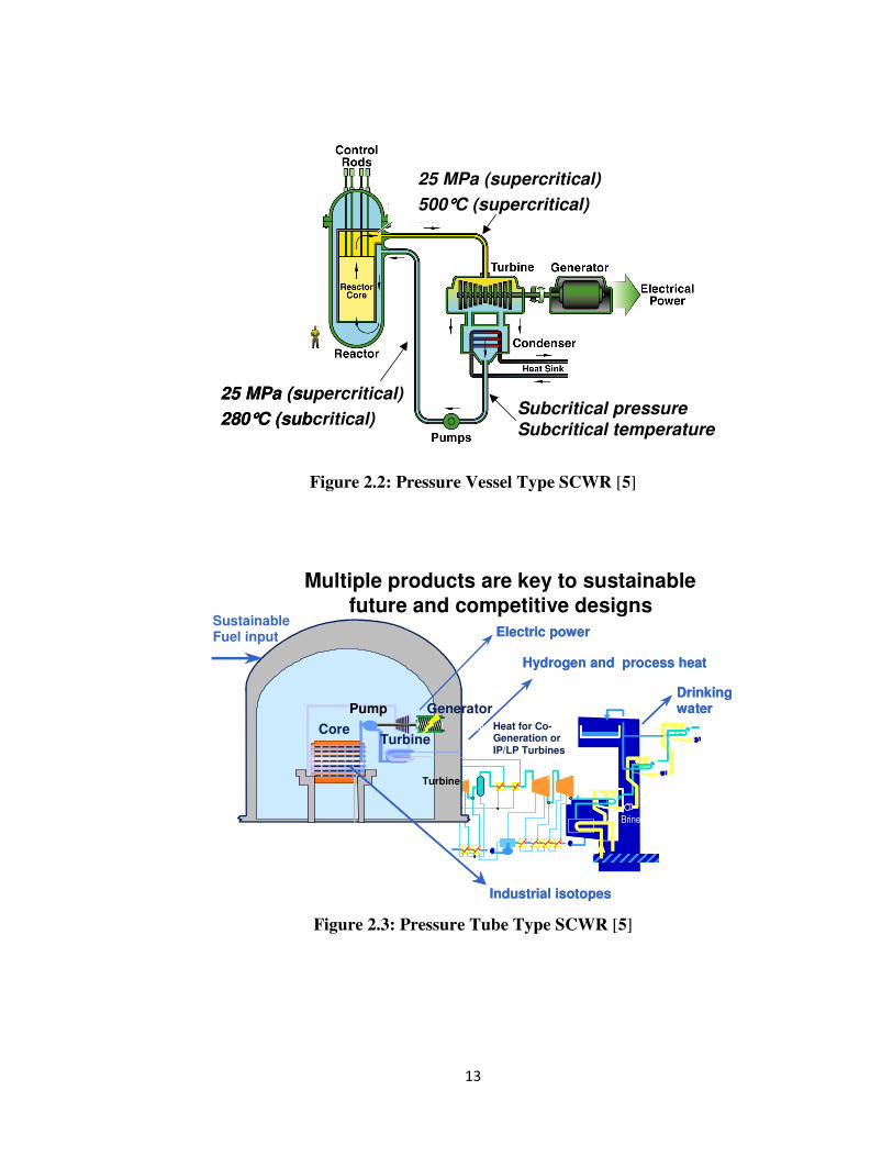
developed worldwide. The PV type reactor as seen in Figure 2.2, is a large reactor

pressure vessel which has a wall thickness of 0.5 m to contain the reactor core. This type

of reactor is analogous to conventional Light Water Reactors and is being developed by

the United States.

The PT reactor, which can be seen in Figure 2.3, is analogous to conventional Heavy

Water Reactors and is designed to be more flexible with respect to flow, flux and density

changes compared to PV reactors. The PT reactor concept is being developed in Canada

12

and Russia by Atomic Energy of Canada Limited (AECL) and the Research and

Development Institute of Power Engineering (RDIPE and NIKIET) respectively [8].

The separation between the moderator and the coolant in the PT SCWR concept allows

for significant enhancement in safety. While SCW is the coolant, various moderator

options are currently being considered.

Three thermodynamic cycle options are being considered for SCWRs. They include the

direct, indirect, and dual cycle options. SC “steam” from the reactor is directly fed to a

SC turbine in the direct cycle. This eliminates the need for steam generators which

results in the highest cycle efficiency among the three cycles. The indirect and dual

cycles use heat exchangers to transfer heat from the reactor to the turbine. Two types of

heat exchangers are being considered: SC water to SC water and SC water to superheated

steam. The maximum temperature of the secondary loop is lower due to heat transfer

through the heat exchangers, hence lowering the efficiency of the cycle [22]. The above

mentioned three options are further divided into various re-heat options. A direct cycle

SCWR with no-re-heat option has been chosen for this analysis and the T-s diagram is

shown in Figure 2.4. Saturated water enters the pump (Point 1), which compresses the

fluid to the supercritical operating pressure. The water is then pre-heated (Point 2 �

Point 3), before it enters the fuel-channel. The coolant continues to be heated as it flows

through the fuel-channel (Point 3 � Point 4). The SC “steam” outlet from the reactor,

which is at pressure of 25 MPa and temperature of 625°C, is then expanded in the SCW

turbine (Point 4 � Point 5) to a sub-atmospheric pressure of 6.77 kPa. The steam is

condensed inside a condenser and enters the pump (Point 5 � Point 1), thus completing

the thermodynamic cycle [23].

13

Figure 2.2: Pressure Vessel Type SCWR [5]

T1, P1

T2, P2

T3, P3

T1, P1

T2, P2

T3, P3

T1, P1

T2, P2

T3, P3

H.P. S

CONDENSER

H.P. S

CONDENSER

Brine

Heat for Co-Generation or IP/LP Turbines

Turbine

Pump Generator

Core

Sustainable

Fuel input Electric power Electric power

Hydrogen and process heat Hydrogen and process heat

Drinking water

Drinking water

Multiple products are key to sustainable

future and competitive designs

Industrial isotopes Industrial isotopes

H.P

Turbine

Figure 2.3: Pressure Tube Type SCWR [5]

25 MPa (supercritical)

500°°°°C (supercritical)


280°°°°C (subcritical)Subcritical pressure

Subcritical temperature


500°°°°C (supercritical)


280°°°°C (subcritical)Subcritical pressure

Subcritical temperature

14

Figure 2.4: T-s diagram for direct cycle SCWR with no-reheat option [23]

15

The main advantage of SCWRs is an increase in thermal efficiency of Nuclear Power

Plants from 30 – 35 % to 45 – 50 % which corresponds to current thermal power plants.

SCWRs operate on a direct cycle where the coolant is the reactor is used in the turbines,

thus eliminating the need for steam dryers, steam heat separators etc., which would lead

to a simplified flow circuit and lower capital and operational costs [5]. SCWRs also have

the ability to facilitate steam based technologies such as desalination, thermochemical

hydrogen production and district heating [24].

Supercritical water has unique thermophysical properties and these properties are

discussed in the following section.

2.3 SCW Properties

The thermophysical properties of supercritical water undergo significant changes within

the critical and pseudocritical regions. The critical point occurs when the distinction

between the liquid and vapour phases disappears and is characterized by Tcr and Pcr. The

critical pressure for water is 22.064 MPa and the critical temperature of water is

373.95°C [4]. The pseudocritical point is a point at a pressure above the critical pressure

and at a temperature corresponding to the maximum specific heat for this particular

pressure [5].

Since SCWRs will operate at a pressure of 25 MPa, the pseudocritical temperature can be

identified by the peak in the specific heat curve shown in Figure 2.5 (a). From Figure 2.5

(a), the pseudocritical temperature corresponds to 384.9°C.

Thermophysical properties such as density, thermal conductivity, dynamic viscosity,

kinematic viscosity, and Prandtl number undergo significant changes in the pseudocritical

region. These changes can be seen in Figure 2.5 (b-f) (Figures constructed using values

extracted from NIST REFPROP at 1°C intervals).

16

350 360 370 380 390 400 410 420 430 440 450

Sp

ecific

He

at [k

J/k

gK

]

0

10

20

30

40

50

60

70

80

Temperature [°C]

pc point P = 25 MPa

Figure 2.5 (a): Specific Heat vs. Temperature of water in the pseudocritical

region at 25 MPa

17

350 360 370 380 390 400 410 420 430 440 450

De

nsity [kg/m

3]

0

100

200

300

400

500

600

700

Temperature [°C]

pc pointP = 25 MPa

Figure 2.5 (b): Density vs. Temperature of water in the pseudocritical

region at 25 MPa

18

350 360 370 380 390 400 410 420 430 440 450

The

rma

l C

on

ductivity,

k [W

/mK

]

0.0

0.1

0.2

0.3

0.4

0.5

0.6

Temperature [°C]

pc pointP = 25 MPa

Figure 2.5 (c): Thermal Conductivity vs. Temperature of water in the

pseudocritical region at 25 MPa

19

350 360 370 380 390 400 410 420 430 440 450

Pra

ndtl N

um

be

r (b

ased

on T

b)

0

1

2

3

4

5

6

7

8

9

10

Temperature [°C]

pc point P = 25 MPa

Figure 2.5 (d): Prandtl Number vs. Temperature of water in the


20

350 360 370 380 390 400 410 420 430 440 450

Dynam

ic V

iscosity

[µP

as]

0

10

20

30

40

50

60

70

80

Temperature [°C]

pc pointP = 25 MPa

Figure 2.5 (e): Dynamic Viscosity vs. Temperature of water in the


21

350 360 370 380 390 400 410 420 430 440 450

Kin

em

atic V

isco

sity [cm

2/s

]

0.0010

0.0015

0.0020

0.0025

0.0030

Temperature [°C]

pc pointP = 25 MPa

Figure 2.5 (f): Kinematic Viscosity vs. Temperature of water in the


22

The most significant changes occur within ±25°C of the pseudocritical temperature.

Properties such as density and dynamic viscosity undergo a significant drop in this region

while there in an increase in the kinematic viscosity. Thermal conductivity and Prandtl

number peak at the pseudocritical point, albeit the peak in the thermal conductivity is

relatively small. As the inlet temperature for a SCWR is 350°C and the outlet

temperature is 625°C, the coolant would pass through the pseudocritical region before

reaching the channel outlet [5]

Various correlations have been developed to calculate the heat transfer characteristics of

supercritical water as shown in the following section.

2.4 SCW Correlations

Dyadyakin and Popov developed a correlation for supercritical water heat transfer for

fuel bundles [25].

�� = 0.0021 ��.� ��.� ��.�� µ�

µ�

��

�.� ��.� �1 + 2.5 �� (2.1)

where � is the axial location along the heated length in metres and �� is the hydraulic

diameter. A tight-lattice, 7 element, helically finned, water-cooled bundle cooled with

water was used to develop the correlation. As heat transfer correlations for bundles are

generally very sensitive to bundle design because of the effect of different bundle

components , and the experiments appear to be for a mobile-type reactor, this correlation

cannot be applied to SCWRs [8].

23

The Dittus-Boelter correlation shown in Equation (2.2) is the most widely used heat

transfer correlation at subcritical pressures for forced convection. The use of this

correlation as shown in Equation (2.2) was proposed by McAdams for forced convective

heat transfer in turbulent flows at subcritical pressures [26].

�� = 0.0243 �� .�� .� (2.2)

Equation (2.2) was later used at supercritical conditions. According to Schnurr et al.,

Equation (2.2) showed good agreement with experimental data for supercritical water

flowing inside circular tubes at a pressure of 31 MPa. It was also noted that the equation

might produce unrealistic results within some flow conditions near the critical and

pseudocritical points but this equation was used as a base for other supercritical heat

transfer correlations [27].

The original Dittus-Boelter correlation shown above is used in the following form for

reference purposes [28]:

�� = 0.023 �� .�� .� (2.3)

Bishop et al. conducted experiments with supercritical water flowing upward inside tubes

and annuli for the following range of operating parameters: pressure: 22.8 – 27.6 MPa,

bulk fluid temperature: 282 – 527°C, mass flux: 651 – 3662 kg/m2s and heat flux : 0.31 –

3.46 MW/m2. Their data for heat transfer were generalized using the following

correlation:

�� = 0.0069 �� .! �� ."" ��.�# �1 + 2.4 �� (2.4)

24

where � is the axial location along the heated length, �� is the density of the fluid at the

wall temperature, �� is the density of the fluid at bulk temperature and the last term

accounts for entrance-region effects [29].

The Bishop et al. correlation is often used without the entrance-region term and is hence

written as:

�� = 0.0069 �� .! �� ."" ��.�# (2.5)

Swenson et al. investigated heat transfer coefficients in smooth tubes and found that

conventional correlations do not work well as they use bulk fluid temperature to calculate

thermophysical properties. The Swenson et al. correlation was developed using a

pressure range of 22.8 – 41.4 MPa, bulk fluid temperature of 75 – 576°C and mass flux of

542 – 2150 kg/m3s. The correlation uses the wall temperature to calculate

thermophysical properties and is shown in Equation (2.6) [30].

��$ = 0.00459 ��$�.!�# ��$�."�# ��.�#� (2.6)

Mokry et al. modified the existing correlations for SCW to obtain a new correlation for

forced-convective heat transfer in a vertical bare tube as seen in Equation (2.7) [8]:

�� = 0.0061 �� .!�� ."�� .�"� (2.7)

Zahlan et al. compared many empirical correlations using a dataset provided by Kirillov

et al. from the Institute of Physics and Power Engineering (Obninsk, Russia) and

concluded that the Mokry et al. correlation is currently the best known correlation for

heat transfer in SCW [31,32].

25

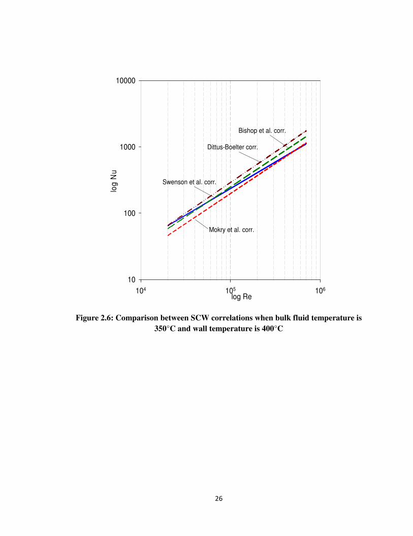
A comparison of the previously mentioned correlations is shown in Figure 2.6. The bulk

fluid temperature was assumed to be 350°C and the wall temperature was assumed to be

400°C. From the figure, it can be seen that the Mokry et al. correlation is the most

conservative of the four correlations shown. Thus, the Mokry et al. correlation will be

used for a conservative analysis in this work. The heat transfer calculations should be

modified as new heat transfer correlations for SCW are published.

26

104 105 106

log

Nu

10

100

1000

10000

log Re

Dittus-Boelter corr.

Bishop et al. corr.

Swenson et al. corr.

Mokry et al. corr.

Figure 2.6: Comparison between SCW correlations when bulk fluid temperature is

350°C and wall temperature is 400°C

27

2.5 Fuel Channel Design Concepts

The current CANDU fuel-channel found in operating CANDU reactors consists of two

tubes, the pressure tube and the calandria tube. The fuel bundles are located within the

pressure tube. An annulus gas gap, which provides thermal insulation, separates the

calandria tube and the pressure tube. The moderator flows outside the calandria tube.

The pressure tube is made from a zirconium niobium alloy while the calandria tube is

made from zirconium [11]. Figure 2.7 shows the present CANDU type fuel-channel.

CANDU 6 reactors have an operating pressure of 9.9 – 11.2 MPa and inlet and outlet

temperatures of 260°C and 310°C respectively while SCWRs will have an operating

pressure of 25 MPa and inlet and outlet temperatures of 350°C and 625°C [11]. The

higher pressures associated with SCWRs are above the pressure tube burst pressure and

thus the current design must be changed.

The current candidate for the CANDU SCWR PT type fuel-channel design uses only a

pressure tube as shown in Figure 2.8. A ceramic liner is used to reduce heat losses to the

moderator. A perforated metal insert is used to protect the ceramic liner from fuel

bundles from scratching during refuelling and also reduce the erosion of the ceramic

liner. The premise for this design is that the metal insert acts as a fuelling sleeve for

transfer of the fuel while the ceramic acts as a thermal barrier. In doing so, the pressure

tube will be at the moderator temperature and the thermal component of pressure tube

creep will be significantly reduced. This design is also called the High Efficiency

Channel (HEC) [9].

Figure 2.7: CANDU

Figure 2.8: SCWR

28

Figure 2.7: CANDU type fuel-channel

Figure 2.8: SCWR type fuel-channel concept

29

While such a design may work, there are concerns with the construction, assembly, and

maintenance of the HEC. One potential problem with this design is that if the ceramic

insulator erodes, fractures, or chips, it might be difficult to repair or replace the ceramic

insulator due to the presence of the metal insert. If deterioration of the ceramic liner was

to occur, then the thermal barrier is weakened and potential hotspots could occur on the

pressure tube. This may result in some of the current problems such as hydriding and

blistering occurring in HEC design. Hence, alternative design concepts that will not have

the above mentioned problem are being considered for the SCWR channel-type reactor.

One such alternative design being considered is called the Re-Entrant Fuel Channel and is

explained in the following Chapter.

30

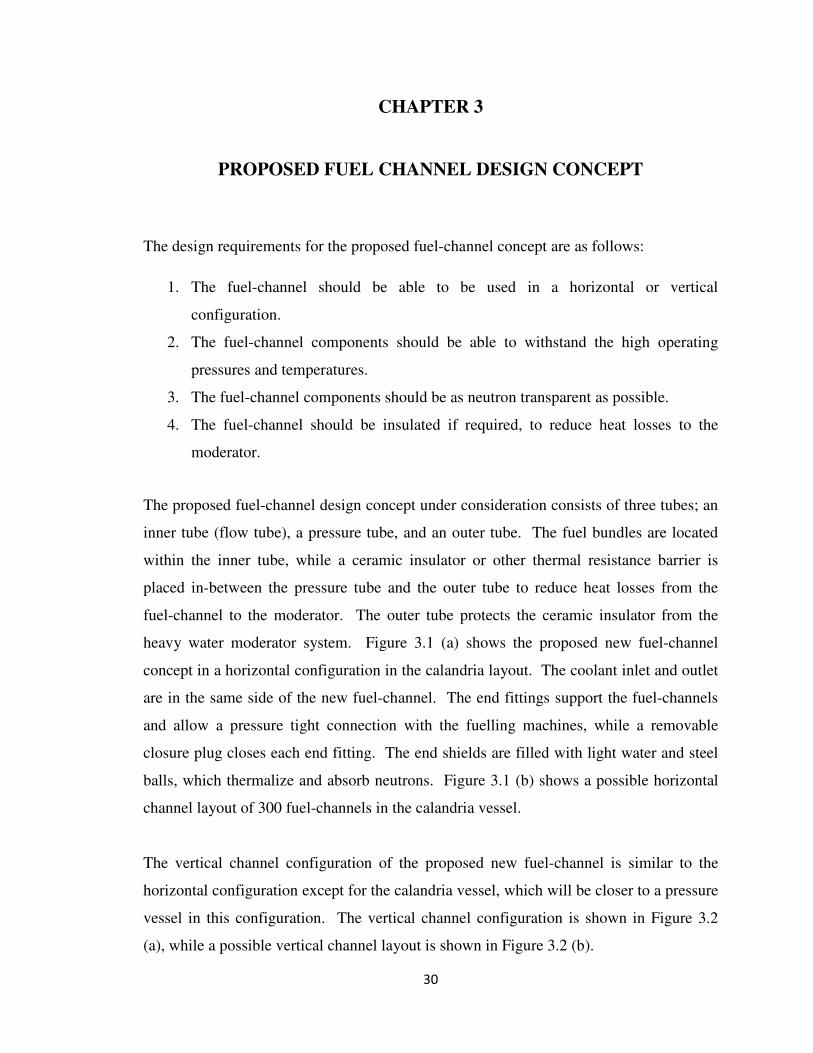
CHAPTER 3

PROPOSED FUEL CHANNEL DESIGN CONCEPT

The design requirements for the proposed fuel-channel concept are as follows:

1. The fuel-channel should be able to be used in a horizontal or vertical

configuration.

2. The fuel-channel components should be able to withstand the high operating

pressures and temperatures.

3. The fuel-channel components should be as neutron transparent as possible.

4. The fuel-channel should be insulated if required, to reduce heat losses to the

moderator.

The proposed fuel-channel design concept under consideration consists of three tubes; an

inner tube (flow tube), a pressure tube, and an outer tube. The fuel bundles are located

within the inner tube, while a ceramic insulator or other thermal resistance barrier is

placed in-between the pressure tube and the outer tube to reduce heat losses from the

fuel-channel to the moderator. The outer tube protects the ceramic insulator from the

heavy water moderator system. Figure 3.1 (a) shows the proposed new fuel-channel

concept in a horizontal configuration in the calandria layout. The coolant inlet and outlet

are in the same side of the new fuel-channel. The end fittings support the fuel-channels

and allow a pressure tight connection with the fuelling machines, while a removable

closure plug closes each end fitting. The end shields are filled with light water and steel

balls, which thermalize and absorb neutrons. Figure 3.1 (b) shows a possible horizontal

channel layout of 300 fuel-channels in the calandria vessel.

The vertical channel configuration of the proposed new fuel-channel is similar to the

horizontal configuration except for the calandria vessel, which will be closer to a pressure

vessel in this configuration. The vertical channel configuration is shown in Figure 3.2

(a), while a possible vertical channel layout is shown in Figure 3.2 (b).

31

The coolant first flows through the gap between the pressure tube and the flow tube from

one end of the channel to the other before reversing direction and flowing through the

inner tube. Thus, the fuel-channel effectively becomes a double-pipe heat exchanger in

which the annulus acts as a preheater. The Re-Entrant channel design is shown in Figure

3.3. The fuel length of the current CANDU-type fuel-channel, 5.772 m, is chosen as the

reference fuel length of the new fuel-channel. The side view of the Re-Entrant channel is

shown in Figure 3.4 (a). The inner tube is referred to as the hot side and the annulus is

referred to as the cold side of the Re-Entrant fuel-channel. Figures 3.4 (b) and (c) show

the entrance region and the re-entrant region of the fuel-channel respectively.

The mass flow rate of the coolant in each channel is 4.37 kg/s [24]. The moderator

temperature is estimated to be 80° C based on current operating parameters. The mean

mass-flow rate of 0.95 kg/s for a mixed type flow in a CANDU-6 reactor is chosen as the

reference mass flow rate of the moderator outside the Re-Entrant channel [33]. The

reference case is a Channel Thermal Power of 8.5 MWth uniformly applied in the fuelled

region. Variable power profiles have also been accounted for in this work.

32

Figure 3.1 (a): Horizontal Re-Entrant channel configuration

Figure 3.1 (b): Horizontal Re-Entrant channel configuration

33

Figure 3.2 (a): Vertical Re-Entrant channel configuration

Figure 3.2 (b): Vertical Re-Entrant channel configuration

34

Fig

ure

3.3

: P

rop

ose

d N

ew F

uel

Ch

an

nel

35

Figure 3.4 (a): Fuel length of Re-Entrant channel

Figure 3.4 (b): Entrance Region of Re-Entrant channel

Figure 3.4 (c): Re-Entrant region of Re-Entrant channel

36

The inner diameter of the flow tube is kept equal to that of the current CANDU-type fuel-

channel for two reasons. The first is that 103.5 mm allows current CANDU-type fuels to

be used in the Re-Entrant channel. The second is that the industry has a lot of

manufacturing and operating experience with this diameter range. The flow tube inner

diameter is a design parameter that could be changed once more knowledge on the

reactor physics and recommended fuel types is known. The four different options for the

fuel bundles are shown in Table 3.1 [34]. They are the 37-Element bundle, the

CANFLEX bundle, the Variant-18 bundle, and the Variant-20 bundle. The 37-Element

and the CANFLEX bundles are currently being used, while the Variant-18 and the

Variant-20 bundle concepts are variations of the CANFLEX bundle that are presently

being developed. The CANFLEX, Variant-18, and the Variant-20 bundles have a total of

43 elements, while the 37-Element bundle has 37 elements. All four fuel bundles contain

four rings of elements and the number of elements in each ring is different for the 37-

Element bundle and the 43 element bundles, as seen in Table 3.1. Unlike the 37-Element

bundle and the CANFLEX bundle, the centre element in the Variant-18 and Variant-20

bundles is unheated and filled with Dysprosium, a burnable neutron absorber which can

reduce void reactivity [35]. The heated length of all four bundles is 481 mm, which

corresponds to a total of 12 bundles in the 5.772 m long Re-Entrant fuel-channel. For the

purposes of this work, the Variant-18 fuel bundle concept has been chosen for the

horizontal Re-Entrant channel configuration. Note that the vertical configuration will use

a fuel string and, depending on the fuelling method, a central rod might be needed to

connect to the fuel string.

37

Table 3.1: Parameters of current fuel bundle options for the Re-Entrant channel

Parameter

Value

37 Element CANFLEX Variant-18 Variant-20

Total No. of Elements 37 43 43 43

No. of elements in the centre

ring

1 1 1 1

No of elements in the inner

ring

6 7 7 7

No. of elements in the

intermediate ring

12 14 14 14

No of elements in the outer

ring

18 21 21 21

Outer diameter of centre ring

element (mm)

13.08

13.5

18.0

20

Outer diameter of inner ring

element (mm)

13.08

13.5

11.5

11.5

Outer diameter of intermediate

ring element (mm)

13.08

11.5

11.5

11.5

Outer diameter of outer ring

element (mm)

13.08

11.5

11.5

11.5

Heated Bundle Length (mm) 481 481 481 481

38

There are few options for the material of construction of the tubes in the Re-Entrant

channel. They include, Zirconium alloy with 2.5 wt% Niobium (Zr-2.5Nb) which is

presently used as the material of construction of CANDU-type pressure tubes, Stainless

Steel – Grade 304 (SS-304), Inconel-718, and a zirconium alloy called Excel (Zr-3.5%

Sn-0.8% Nb–0.8% Mo-1130 ppm O). The Ultimate Tensile Strength (UTS) for all of the

above mentioned materials is similar for the operating range of the Re-Entrant fuel-

channel. Tests have shown that the creep rate in Excel is much lower than Zr-2.5Nb,

however Zirconium alloys are not suitable for long term exposure to supercritical water

unless they are coated to avoid corrosion [9]. There is little data for irradiation creep and

swelling at the high temperatures associated with the Re-Entrant fuel-channel for all of

the above mentioned materials [6]. Extensive testing needs to be conducted using all four

materials before the design of the Re-Entrant channel is finalized. For the purpose of this

work, SS-304 has been chosen as the material of construction of the inner tube, the

pressure tube and the outer tube.

The inner tube in the Re-Entrant channel can be made as thin as possible to improve

neutron economy as it is not required to bear any significant pressure difference[9]. A

reference thickness of the inner tube is 2 mm, and a sensitivity analysis on the thickness

of the inner tube is performed in Chapter 5. The inner diameter of the pressure tube is

calculated to be 127.9 mm. ASME standards require that the design stress of the pressure

boundary component be less than 1/3 of the UTS of the material [9]. The UTS of SS-304

at 400°C is 448 MPa [36]. Analysis in Chapter 5 indicate that the actual temperature of

the pressure tube is much lower than 400°C, but the UTS of SS-304 is chosen at this

temperature to account for a reasonable safety factor. Thus, the minimum thickness of

the pressure tube required to satisfy the ASME standards is 10.71 mm. The reference

pressure tube thickness for this work is chosen to be 11 mm.

An insulator is required so that only 1 to 2 % of the thermal energy would be lost to the

moderator from the Re-Entrant channel. Two different ceramic insulators are chosen in

this work. The first is the ceramic insulator which is used in the HEC channel, so that

heat loss comparisons can be made between the two designs. Thus, Porous Yttria

39

Stabilized Zirconia (with 70% porosity) has been chosen as for the insulation. Unlike the

HEC channel, the Re-Entrant channel does not have SCW flowing through the pores of

the insulator as the insulator is placed outside the pressure tube. Carbon dioxide (CO2)

gas flows through the pores in the insulator. Similar to current CANDU-type reactors,

the moisture content of the CO2 gas can be analyzed to determine if there is a leak in the

pressure tube. Yttria Stabilized Zirconia (YSZ) has a low neutron cross section and low

thermal conductivity. Studies have shown that irradiation would not significantly

embrittle YSZ at high temperature [37]. Porous YSZ, with open pores increases the

thermal resistance and improves the thermal shock resistance. The other insulating

option selected for the Re-Entrant channel is solid zirconium dioxide (ZrO2). The solid

insulator eliminates the need for the CO2 gas system. The reference thickness of the

insulator is 7 mm and a sensitivity analysis on the insulator thickness can be seen in

Chapter 5, along with a detailed comparison of the performance of both insulators

selected for use in the Re-Entrant channel. The rear end of the Re-Entrant channel will

be insulated in the end shield of the calandria.

The main purpose of the outer tube is to prevent erosion of the ceramic insulator in the

moderator. Hence, the outer tube can be as thin as possible to improve neutron economy

and the reference thickness of the outer tube is 0.5 mm. Table 3.2 shows the relevant

dimensions associated with the Re-Entrant channel and Figure 3.5 shows the cross-

sectional view of the channel.

40

Table 3.2: Reference case Re-Entrant Channel Dimensions

Parameter Value

Flow tube – Inner Diameter (mm) 103.5

Flow tube – Outer Diameter (mm) 107.5

Pressure tube – ID (mm) 127.9

Pressure tube – OD (mm) 149.9

Ceramic thickness (mm) 7

Outer tube – ID (mm) 163.9

Outer tube – OD (mm) 164.9

Notes: Flow tube, pressure tube, ceramic insulation and outer tube thicknesses may vary as a

design option.

Figure 3.5: Cross sectional view of Re-Entrant channel

41

Unlike present CANDU reactors, the REC uses the “fuel against flow method” and can

only be refuelled from one end. The single-ended refuelling concept was developed for

the CANDU-3 and CANDU-80 reactor designs for fuel bundles, and experimentally

demonstrated on a full-scale mockup. In single-ended refuelling, a refuelling machine

pushes the bundles to the end of the channel, where a bundle stopper is present. This

stopper prevents the fuel bundles from sliding during normal operation. Once the bundle

has reached the end of a channel, the machine engages a latch at the front end, which

keeps the bundles from sliding forward. When the bundles need to be removed from the

channel, the refuelling machine disengages the latch, while the force of the coolant

pushes the bundles out. For a vertical configuration, a fuel string is used. Refuelling of a

vertical channel has been demonstrated for several reactor types as NRU, Gentilly-1 and

RBMK.

The main advantage of the Re-Entrant channel is the elimination of the ceramic liner

inside the fuel-channel where the pressures and temperatures are considerably higher than

the outside of the pressure tube. This means that the ceramic insulator will never come in

contact with the coolant, hence avoiding the problem of having eroded ceramic particles

in the primary heat transport system. Another advantage of the Re-Entrant channel over

the HEC is that if there is an issue with the ceramic in the HEC, the entire fuel-channel

assembly needs to be taken apart to examine the ceramic insulator, and this will not be an

easy process if the fuel-channel is irradiated. This will not be the case in the Re-Entrant

channel as the ceramic liner is outside the pressure tube. The Re-Entrant channel can be

used in both the horizontal and vertical channel configurations whereas the HEC is

designed for use in the horizontal configuration. The location of the pseudocritical point

in the REC could also be an advantage if it occurs in the cold side of the fuel-channel as

it’s separate from the fuelled region. This may address concerns with deteriorated heat

transfer and chemistry control in the pseudocritical region. One possible disadvantage of

the Re-Entrant fuel-channel is that the piping and fittings would be congested as the inlet

and outlet are at the same side of the channel [9]. Another disadvantage of the Re-

Entrant channel is that it may lead to bigger calandria vessels to accommodate the larger

fuel-channels.

42

CHAPTER 4

NUMERICAL MODEL OF RE-ENTRANT FUEL-CHANNEL

This chapter discusses the fundamental theory and how it is applied to develop a

numerical model that represents the proposed fuel-channel.

4.1 Fundamental Equations

Fourier’s law states that for one-dimensional steady-state conduction in a plane wall with

no heat generation and constant thermal conductivity, the temperature varies linearly with

the thickness, �, as shown in Equation (4.1) below:

� = − � %�%� (4.1)

where is the thermal conductivity and A is the cross-sectional surface area [38].

Newton’s law of cooling is used to find the heat transfer through convection and is shown

in Equation (4.2) [38].

� = ℎ�∆� (4.2)

where ℎ is called the convective heat-transfer coefficient.

The conservation of mass relation for a two-dimensional steady flow of a fluid is given

by Equation (4.3) [39].

&'&� +

&(&) = 0 (4.3)

43

where the �-component of the velocity is � and the �-component is �.

The conservation of momentum in the �-direction or the �-momentum equation is given

by Equation (4.4) [39].

� �� &'&� + � &'

&)� = � &�'&)� −

&*&� (4.4)

where � is the density of the fluid, � is the dynamic viscosity and � is the pressure.

During a steady-flow process, the total energy content of a control volume remains

constant, and the amount of energy entering a control volume in all forms equals the

amount of energy leaving it. This implies that the net energy convected by a fluid out of

a control volume is equal to the net energy transferred into the control volume by heat

conduction and the energy equation for a two-dimensional steady flow of a fluid with

constant properties is given by Equation (4.5) [39].

��+ �� &�&� + � &�

&)� = �&��&�� +&��&)�� (4.5)

where �� is the specific heat. The above equations can be written in a

nondimensionalized form that can be used to derive the Nusselt number (��), which

represents the enhancement of heat transfer through a fluid layer as a result of convection

relative to conduction. The Nusselt number is referred to as the dimensionless heat

transfer coefficient and can be expressed in terms of the Reynolds number ( !) and

Prandtl number (�") and hence Equation (2.7) can be used along with Equation (4.2) to

find the heat transfer through a fluid.

44

4.2 Flow Area, Wetted Perimeter, Hydraulic Diameter

Since the diameters of the elements in the bundles are known, the cross-sectional area of

the fuel bundle can be calculated using Equation (4.6).

A� =,� ��D�-�� + 42 �D- �� ; �� (4.6)

The cross-sectional area of the flow tube can be found using Equation (4.7). The

difference between the cross-sectional area of the flow tube and the bundles gives the

flow area of the inner tube as seen in Equation (4.8).

A�� =

,� ��D.�� ; �� (4.7)

A/ = A�� − A� ; ��

A/ =,� ��D�-�� + 42 × �D- �� − �D.�� ; �� (4.8)

The hydraulic diameter of the inner tube can be calculated using the following equation:

D0) � = 41�*�� ; �� (4.9)

where the wetted perimeter (�234) can be calculated using Equation (4.10).

P$56 = � ��D�-� + 42 × �D- � + D.�� ; �� (4.10)

45

The flow area of the annulus is given by:

A/� =,� �D.��

� − D7�� ; �� (4.11)

The hydraulic diameter of the annulus can be found using Equation (4.12).

D0)� = ��89��

��9�� :

,9�� ; ,9�� ; ��

D0)� = D.�� − D7�� ; �� (4.12)

The mass fluxes of the inner tube and the annulus can be calculated by using Equation

(4.13) and Equation (4.14) respectively.

G<� =�=>�

; � �� (4.13)

G1 =�=

>�� ; � �� (4.14)

46

Table 4.1: Reference case Re-Entrant Channel Parameters

Parameter Value

Wetter perimeter of Variant-18 bundle (m) 1.5174

Cross-sectional fuelled area of bundle (m2) 0.0046

Cross-sectional flow area of inner tube (m2) 0.0084

Wetted perimeter of inner tube (m) 1.8989

Hydraulic diameter of inner tube (m) 0.0080

Mass flux of inner tube (kg/m2s) 1153.6

Flow area of annulus (cold side) (m2) 0.0038

Hydraulic diameter of annulus (cold side) (m) 0.0205

Mass flux of annulus (cold side) (kg/m2s) 1153.6

47

4.3 Nodalization

To apply the heat balance model using the fundamental equations in Section 4.1, the fuel-

channel needs to be divided into several nodes. The pressure is assumed to be constant in

this model at 25 MPa. For the purpose of this work, the Re-Entrant channel was divided

into 121 nodes; 60 for the cold side, 60 for the hot side and one for the re-entrant mixing

node which is the region where the coolant from the annulus changes direction and flows

in the inner tube. The coolant inlet temperature boundary condition is a temperature of

350°C and the coolant outlet temperature is initially assumed to be 625°C. The

temperature of the mixing node is initially assumed to be 400°C. Figure 4.1 shows the

nodes in the Re-Entrant fuel-channel along with the initial estimates of the coolant exit

temperature and the mixing node.

4.4 Initial Estimate of Temperature profiles for Hot and Cold Side

With the three temperatures shown in Figure 4.1, the temperature profile for the coolant

for the Re-Entrant fuel-channel can initially be assumed to be linear.

48

Fig

ure

4.1

: R

e-E

ntr

an

t fl

ow

ch

an

nel

sh

ow

ing

no

des

an

d i

nit

ial

tem

per

atu

re e

stim

ate

s

49

4.5 Initial Estimate of Temperature of Fuel Sheath

The temperature of the fuel sheath in each node is initially assumed to be 300°C higher

than the temperature of the hot coolant. Since the pressure at the node is known, the bulk

fluid enthalpy of the coolant, enthalpy of the coolant at the wall, i.e. fuel sheath, density

of the bulk fluid, and the density of the coolant at the wall, can be obtained using NIST

REFPROP, along with the thermal conductivity and viscosity of the coolant in the hot

side.

As the wall temperature of the outer sheath is much higher than the coolant in the hot

side, the average specific heat and average Prandtl numbers are used to calculate the flow

parameters of the hot coolant as they account for the difference in temperature. The

average specific heat and the average Prandtl number for each node in the hot side can be

calculated using the following equations:

�̅+ =�� ; � �

��∙�� (4.15)

�� = ?��∙��̅�� (4.16)

Equation (4.17) below is used to calculate the Reynolds number of the coolant in the hot

side.

�� = � ∙9��

?�� (4.17)

With the above equations for the Reynolds and Prandtl numbers, the Nusselt number can

be calculated using Equation (2.7). The convection heat transfer coefficient can be

calculated using Equation (4.18).

50

ℎ0 = �� 9��

; � ��∙�� (4.18)

The fuel sheath temperature is calculated using the equation below [28]:

�/ =@0�� + �0 ; [°�] (4.19)

Since the fuel sheath temperature was first estimated to be 300°C higher than the hot

coolant and the above equation calculates the temperature of the fuel sheath based on that

estimate, the above process is repeated until the value of one iteration and the value of the

previous iteration are within 0.1°C of each other to determine the actual estimate of the

fuel sheath temperature.

4.6 Thermal Resistances

The thermal resistance of the hot fluid can be calculated using Equation (4.20).

0 =�

0��1 � ; �°�� (4.20)

Equation (4.21) can be used to calculate the thermal resistances of the flow tube, the

pressure tube, and the outer tube.

6' 5 =AB (

��

)

�,C� ; �°�� (4.21)

The thermal conductivity of SS-304 is calculated using Equation (4.22) [40].

DD�#�� = 2.0 ∙ 10�"�� + 0.0134 � + 10.689 ; � ��∙�� (4.22)

51

The heat transfer coefficient for the cold side can be calculated using Equations (4.15) to

(4.18) by using the appropriate thermophysical properties for the cold side, which can be

obtained from NIST REFPROP. Once the heat transfer coefficient for the cold side is

known, the thermal resistance for the cold fluid can be calculated using the following

equation:

� =�

0��1�� ; �°�� (4.23)

A rough upper-bound estimate of the thermal conductivity of Porous YSZ (70% porosity)

is given by Equation (4.24) [9].

EDF = 0.3 kFGH� + 0.7 �H�; � ��∙�� (4.24)

The average thermal conductivity of �� is 2.7 (�/� ∙ #) in the temperature range of

this analysis. The thermal conductivity of carbon dioxide is a function of temperature

and the thermal conductivity of the Porous YSZ insulation with �� is shown in

Figure 4.2.

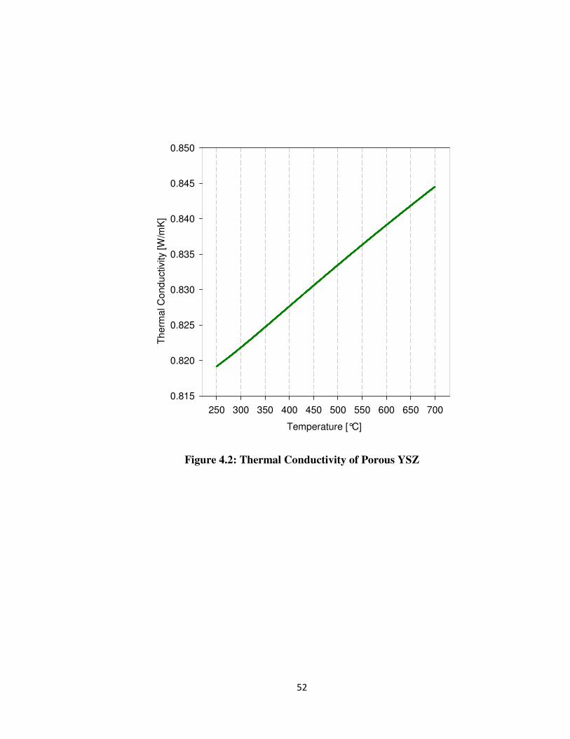
52

Temperature [°C]

250 300 350 400 450 500 550 600 650 700

Th

erm

al C

ond

uctivity [W

/mK

]

0.815

0.820

0.825

0.830

0.835

0.840

0.845

0.850

Figure 4.2: Thermal Conductivity of Porous YSZ

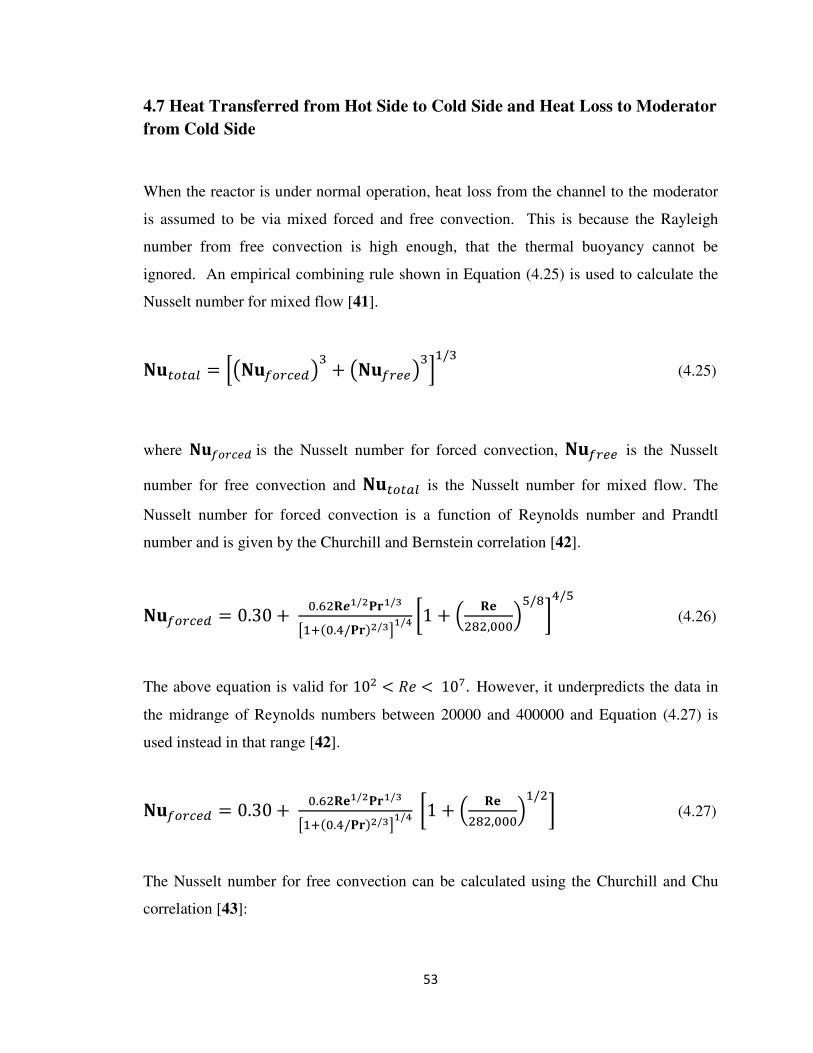
53

4.7 Heat Transferred from Hot Side to Cold Side and Heat Loss to Moderator

from Cold Side

When the reactor is under normal operation, heat loss from the channel to the moderator

is assumed to be via mixed forced and free convection. This is because the Rayleigh

number from free convection is high enough, that the thermal buoyancy cannot be

ignored. An empirical combining rule shown in Equation (4.25) is used to calculate the

Nusselt number for mixed flow [41].

��676IJ = ��/7G�5%�# + ��/G55�#��/# (4.25)

where �� is the Nusselt number for forced convection, ��/G55 is the Nusselt

number for free convection and ��676IJ is the Nusselt number for mixed flow. The

Nusselt number for forced convection is a function of Reynolds number and Prandtl

number and is given by the Churchill and Bernstein correlation [42].

��/7G�5% = 0.30 + �."�KL�/��/�

M�;��.�/��/�N�/� !1 + � KO��,��/�"�/�

(4.26)

The above equation is valid for 10� < ! < 10�. However, it underpredicts the data in

the midrange of Reynolds numbers between 20000 and 400000 and Equation (4.27) is

used instead in that range [42].

��/7G�5% = 0.30 + �."�KO�/��/�

M�;��.�/��/�N�/� !1 + � KO��,��/�" (4.27)

The Nusselt number for free convection can be calculated using the Churchill and Chu

correlation [43]:

54

��/G55 = #0.60 +�.#�"KP��/�

Q�;R�.��

!S�/��T

"/�#$�

(4.28)

The Rayleigh number can be calculated using Equation (4.29) [28].

�% = ��

�U (4.29)

Once the temperature of the coolant at each node is known, and the total thermal

resistances of the fuel-channel components are calculated, the heat loss to the moderator

and the heat transferred from the hot side to the cold side can be calculated using:

� =∆�

V��$% ; [�] (4.30)

= ��

;[�] (4.31)

=��

�

��

�� (��

)

��

� �

�� (

��

)

��

�� (��

)

��

�� (��

)

��

� �

��

;�� (4.32)

4.8 Actual Temperature Profile of Cold Side, Hot Side & Fuel Sheath

The net heat loss is the difference between the heat transferred to the cold side from the

hot side and the heat loss to the moderator. Since the pressure and temperature of the first

node for the cold side is known, the enthalpy of Node 1 can be obtained from NIST

REFPROP. Equation (4.33) can be used to calculate the enthalpy of the next node.

&W,.;� (�7J%) = &W,. +@��(�)

�= ; � �� (4.33)

55

The above equation is slightly modified to calculate the enthalpy of the hot side to

account for different power profiles.

&W,.;� (076) = &�,. +X�&�∙+∙∆�

�= ; � �� (4.34)

Once the enthalpies for the hot and cold sides are calculated at each node, the temperature

profiles for the coolant can be obtained from NIST REFPORP. With the actual

temperature profile of the hot side, Equations (4.15) to (4.19) can be used to calculate the

actual temperatures of the fuel sheath.

4.9 Surface Temperatures of Tubes

Equation (4.30) can also be used to calculate the inner and outer surfaces temperatures of

the inner, pressure and outer tubes.

4.10 MATLAB code

A numerical model was developed using the equations shown above and a program was

written in MATLAB to calculate the heat-transfer characteristics of the Re-Entrant fuel-

channel. Figure 4.3 is a flow chart that highlights the main steps in the code, which is

shown in Appendix A.

Figure 4.3: Flow chart representing Numerical Model in MATLAB

56

: Flow chart representing Numerical Model in MATLAB

: Flow chart representing Numerical Model in MATLAB

57

CHAPTER 5

HEAT TRANSFER ANALYSIS

Numerical analysis was done for several different parameters to study their effect on heat

transfer. The objective is to determine the sensitivity of the design to the tube thickness,

and material choice by using the thermal conductivity. The effect of the insulator design

on heat loss and the impact of variable heat flux profiles are considered. The impact of

the location of the pseudocritical point and the location of peak fuel sheath temperature is

assessed in each case.

5.1 Reference Case: No Heat Loss to the Moderator

Heat-transfer analysis was performed on the Re-Entrant channel assuming no heat loss to

the moderator. This case is ideal from the heat loss perspective and will result in the

highest fuel temperature and highest coolant temperature. The fuel-channel power, the

thickness of the flow tube, and the flow-tube thermal conductivity were varied for this

analysis, while heat flux was assumed to be constant. The coolant enters the cold side of

the Re-Entrant channel at x = 5.772 m, and enters the hot side at x = 0 m, as shown in

Figure 4.1.

Figure 5.1 shows the axial temperature profiles of the coolant, the inner and outer

surfaces of the flow tube and the outer fuel sheath along the heated length of the channel

for a channel power of 8.5 MWth, a coolant inlet temperature of 350°C, a mass flow rate

of 4.37 kg/s, and uniform heat flux. The pressure tube is not included in the analysis and

no heat transfer from the cold coolant side to the pressure tube is allowed. The

temperature of the coolant on the cold side increases approximately linearly, as expected,

as the heat source is the outer wall of the flow tube. The coolant temperature on the hot

side increases slowly at first and then dramatically after approximately 2 m of fuelled

length. The main reason for this, as will be seen in later figures, is the transition of the

58

coolant through the pseudocritical point. The pseudocritical temperature for light water

at 25 MPa is 384.9°C. The outer-sheath temperature increases at first, decreases and

then increases again. This behaviour is expected for a uniform heat flux and constant

mass flux as there is a significant improvement in heat transfer as the coolant passes

through the pseudocritical point [44]. The outer sheath temperature is below the design

limit of 850°C. This case will be used as the reference case for the remainder of the

analysis.

59

Channel Length [m]

0.000 0.962 1.924 2.886 3.848 4.810 5.772

Tem

pera

ture

[°C

]

300

400

500

600

700

800

900

Coolant (Hot Side)

Coolant (Cold Side)

Tpc = 384.9°C

Outer Sheath

FTi

FTo

Sheath Temp Limit = 850°C

Figure 5.1: Axial temperature profile along the fuelled channel length for a channel

power of 8.5 MWth, inner-tube thickness of 2 mm, inlet temperature of 350°C, mass

flow rate of 4.37 kg/s and uniform heat flux

60

The location of the pseudocritical point in the channel can be identified by the peak in the

specific heat profile for the coolant as shown in Figure 5.2. Thermophysical properties

such as thermal conductivity, Prandtl number, and specific heat drastically change within

the pseudocritical region, as seen in Figure 5.2. These changes result in the variation in

slopes of the coolant temperature and outer sheath temperature profiles at these locations

in Figure 5.1. The thermophysical properties shown in Figure 5.2 are calculated using the

bulk-fluid temperature along the channel. The thermal conductivity of the coolant

decreases slightly along the cold side of the channel. Once the coolant enters the hot

side, the thermal conductivity decreases significantly due to the higher bulk fluid

temperatures of the coolant, before being almost constant just before the pseudocritical

point. The thermal conductivity decreases drastically once the coolant becomes

supercritical. The specific heat and Prandtl number profiles slightly increase as the

coolant passes thought the cold side of the fuel-channel. As the coolant enters the fuelled

region, the profiles increase drastically up to the pseudocritical point when the coolant

enters the fuelled region due to higher bulk fluid temperatures, and then decrease until to

the end of the hot side of the fuel-channel.

The average Prandtl number and average specific heat from Equations 4.15 and 4.16 were

calculated using the bulk-fluid and wall temperatures and the resulting profiles are shown

in Figure 5.3. The heat transfer coefficient profile which is calculated using Equation

4.13 is also shown in Figure 5.3 along with the heat flux for the hot side. The average

specific heat is the ratio between the difference in the enthalpies of the coolant at the wall

temperature and the bulk fluid temperature to the difference in the temperature of the

coolant at the wall and the bulk fluid temperature. As the coolant enters the fuelled

region, there is an increase in the wall temperature of the fuel sheath and the enthalpy of

the coolant at the wall. This accounts for the significant increase in the specific heat

profile at the entrance of the hot side. The average Prandtl number is directly

proportional to the average specific heat. Thus, there is also a significant increase in the

average Prandtl number profile.

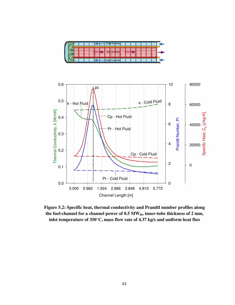
61

Channel Length [m]

0.000 0.962 1.924 2.886 3.848 4.810 5.772

Th

erm

al C

on

du

ctivity,

k [W

/mK

]

0.0

0.1

0.2

0.3

0.4

0.5

0.6

Pra

nd

tl N

um

be

r, P

r

0

2

4

6

8

10

Sp

ecific

He

at, C

p [J/k

g·K

]

0

20000

40000

60000

80000

k - Cold Fluidk - Hot Fluid

Pr - Cold Fluid

Pr - Hot Fluid

Cp - Cold Fluid

Cp - Hot Fluid

pc

Figure 5.2: Specific heat, thermal conductivity and Prandtl number profiles along

the fuel-channel for a channel power of 8.5 MWth, inner-tube thickness of 2 mm,


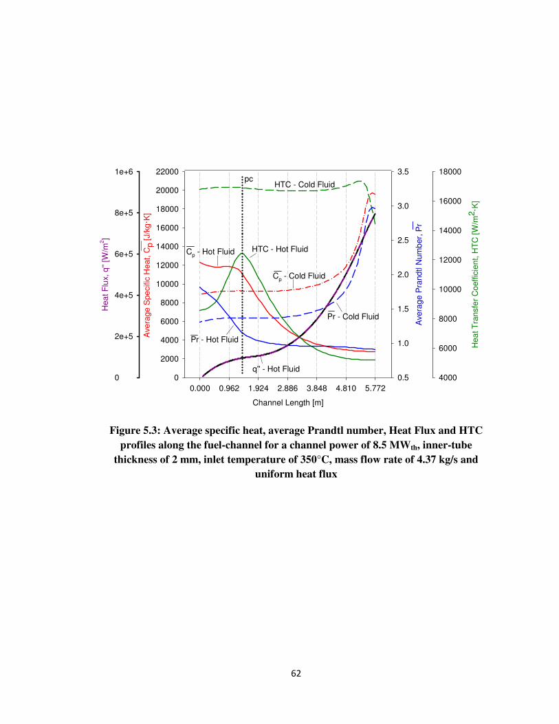
62

Channel Length [m]

0.000 0.962 1.924 2.886 3.848 4.810 5.772

Avera

ge S

pecific

Heat, C

p [J/k

g·K

]

0

2000

4000

6000

8000

10000

12000

14000

16000

18000

20000

22000

Hea

t T

ransfe

r C

oeffic

ient, H

TC

[W

/m2·K

]

4000

6000

8000

10000

12000

14000

16000

18000

Avera

ge P

randtl N

um

ber,

Pr

0.5

1.0

1.5

2.0

2.5

3.0

3.5

Hea

t F

lux, q''

[W/m

2]

0

2e+5

4e+5

6e+5

8e+5

1e+6

HTC - Cold Fluid

HTC - Hot Fluid

Cp - Cold Fluid

Cp - Hot Fluid

Pr - Cold Fluid

Pr - Hot Fluid

pc

q'' - Hot Fluid

Figure 5.3: Average specific heat, average Prandtl number, Heat Flux and HTC

profiles along the fuel-channel for a channel power of 8.5 MWth, inner-tube


uniform heat flux

63

Not all fuel-channels have the same power in the core. Refuelling and balancing the

neutron flux are two instances where fuel-channel power is varied among the fuel-

channels in the core. The effect of power on the outer sheath temperature profile is

shown in Figure 5.4. As expected, the maximum outer sheath temperature at the outlet of

the fuelled region (hot side) increases with increasing power. This also means the coolant

will reach the pseudocritical region earlier along the axial length of the channel with

increasing power. Thus, the pseudocritical point shifts along the channel from the outlet

towards the inlet with increasing channel power as shown in Figure 5.4.

As there is no pressure boundary requirement for the flow tube, the thickness of the flow

tube is dominated by heat transfer characteristics and physical strength. The reference

flow tube thickness for this analysis was chosen to be 2 mm. As this work only consisted

of a heat transfer analysis, the flow tube thickness might change once a detailed analysis

on the physical strength of the REC is performed. A sensitivity analysis for variable

thickness of the flow tube was performed and Figure 5.5 shows the variation of the outer-

sheath temperature for flow tube thicknesses of 2 mm, 3 mm and 5 mm. Thicker tubes

reduce neutron economy, but they may reduce the heat transfer characteristics of the hot

fluid. However, there is a very slight difference in the outer sheath temperature for all

three cases as seen in Figure 5.5. This suggests that the heat transfer is not significantly

affected by the thickness of the inner flow tube, and thus, the thickness of the inner flow

tube can be determined by neutron economy.

64

Channel Length [m]

0.000 0.962 1.924 2.886 3.848 4.810 5.772

Oute

r S

he

ath

Te

mpe

ratu

re [°C

]

300

400

500

600

700

800

900

Hea

t T

ransfe

r C

oeffic

ien

t, H

TC

[W

/m2·K

]

4000

6000

8000

10000

12000

14000

16000

18000

20000

22000

24000

26000

Outer Sheath Temp: 8.5 MW

HTC: 8.5 MW

pc (8.5 MW)


HTC: 5.5 MW

pc (5.5 MW)

Outer Sheath Temp: 5.5 MW

Figure 5.4: Outer-sheath-temperature profile along the channel length for powers of

8.5 MWth and 5.5 MWth, inner-tube thickness of 2 mm, inlet temperature of 350°C,


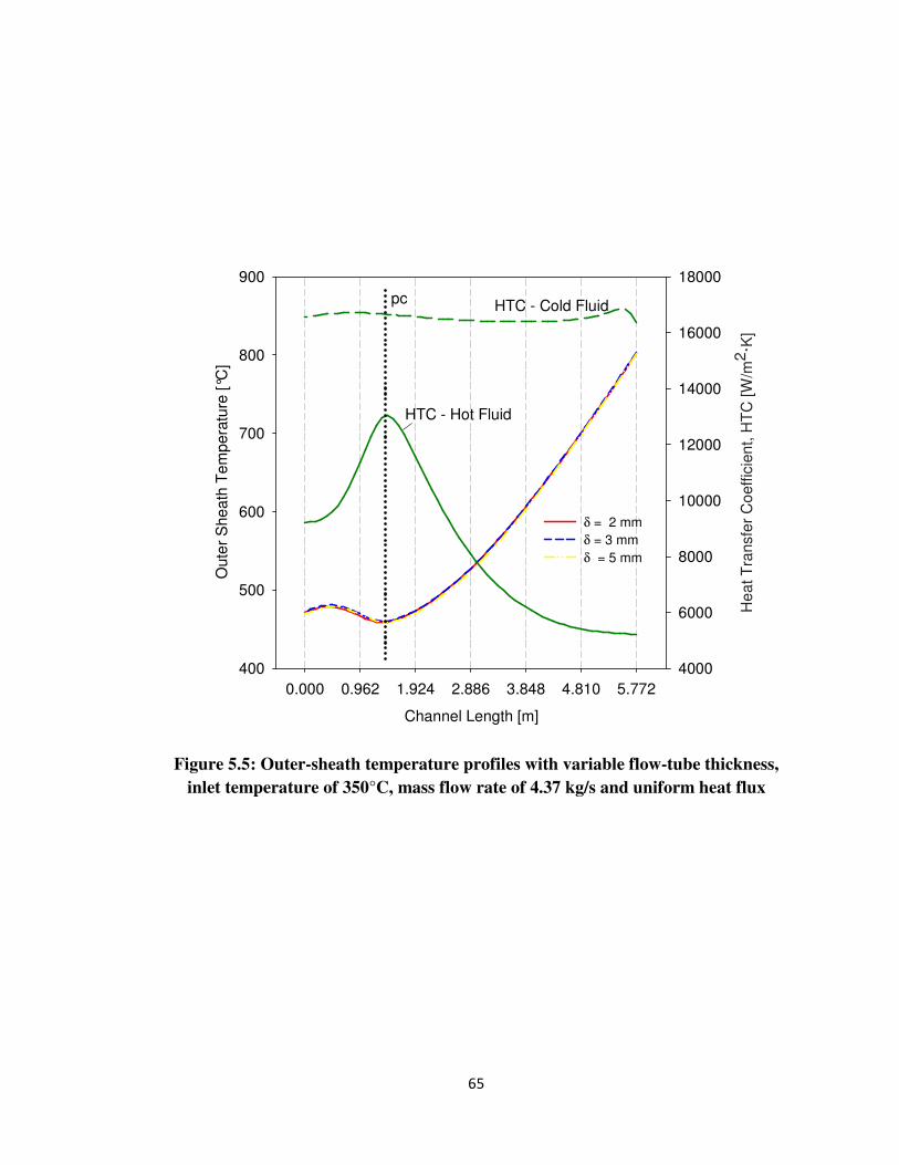
65

Channel Length [m]

0.000 0.962 1.924 2.886 3.848 4.810 5.772

Oute

r S

he

ath

Te

mp

era

ture

[°C

]

400

500

600

700

800

900

He

at T

ransfe

r C

oeffic

ien

t, H

TC

[W

/m2

·K]

4000

6000

8000

10000

12000

14000

16000

18000

δ = 2 mm

δ = 3 mm

δ = 5 mm

HTC - Cold Fluid

HTC - Hot Fluid

pc

Figure 5.5: Outer-sheath temperature profiles with variable flow-tube thickness,


66

The thermal resistance of the inner tube is inversely proportional to the thermal

conductivity of the material of construction, and directly proportional to the change in

temperature across the inner tube. The higher the thermal conductivity of the inner tube,

the larger the temperature difference across the inner tube. This also means that more

heat will be transferred from the hot side to the cold annulus. Figure 5.6 shows the

change in temperature across the inner tube with various wall thermal conductivities.

The figure indicates that the wall thermal conductivity will be an important consideration

for the flow as it will define the heat transfer to the cold annulus of the flow channel.

Changing the inner tube material does not have the same effect on the outer sheath

temperature as it does on the temperature difference across the inner tube. The change in

the outer-sheath temperature for various wall thermal conductivities is nearly constant

when the reference conductivity is multiplied by a factor of 0.5 and 2 as shown in Figure

5.7. The results indicate that the heat transfer characteristics of the flow tube will not

significantly affect the ability to cool of the fuel. The main reason for this is that heat

loss to the cold annulus is low, and also, the cold annulus is essentially acting as a fluid

preheater, and the lost heat is recovered.

67

0.000 0.962 1.924 2.886 3.848 4.810 5.772

∆T

acro

ss Inn

er

Tu

be

[°C

]

0

20

40

60

80

100

120

Reference Thermal Conductivity of Inner Tube

Thermal Conductivity of Inner Tube changed by a factor of 0.5

Thermal Conductivity of Inner Tubechanged by a factor of 2

Channel Length [m]

Figure 5.6: Change in temperature across the flow tube for different wall thermal

conductivities, inner-tube thickness of 2 mm, inlet temperature of 350°C, mass flow


68

Channel Length [m]

0.000 0.962 1.924 2.886 3.848 4.810 5.772

Oute

r S

hea

th T

em

pe

ratu

re [°C

]

400

500

600

700

800

900

He

at T

ransfe

r C

oeffic

ien

t, H

TC

[W

/m2

·K]

4000

6000

8000

10000

12000

14000

16000

18000

Reference k

k x 0.5

k x 2

HTC - Cold Fluid

HTC - Hot Fluid

pc

Figure 5.7: Temperature Profile of Outer Sheath Temperature for variable wall

thermal conductivity, inner-tube thickness of 2 mm, inlet temperature of 350°C,


69

The heat-transfer analysis performed for the reference Re-Entrant channel assumes no

heat loss to the moderator. The temperature profiles of the coolant, outer sheath, inner

surface of the flow tube and outer surface of the flow tube were estimated at different

operating conditions. The temperature profiles of the coolant in the hot side and of the

outer sheath change considerably within the pseudocritical region. The pseudocritical

point occurs close to the entrance of the coolant into the flow tube, approximately near

fuel bundle #3 for the reference case. The location of the pseudocritical point changes

with channel power as expected, but is not significantly affected by the wall thickness of

the inner tube or the thermal conductivity of the inner tube. Note that with significant

overpower, it may be possible for the pseudocritical point to move to a region upstream

of the fuelled length as seen in Figure 5.8 when the channel power is 10 MW. For this

case, the location of the pseudocritical moves from � = 1.54 m to � = 1.2506 m. This

shows that at 10 MWth, the pseudocritical point is still in the hot side of the fuel-channel.

However, the outer sheath temperature is much higher than the sheath temperature limit

indicating that the outer sheath may melt. The coolant exit temperature also is over 100°C

higher than the desired exit temperature of 625°C.

In reality, there are heat losses to the moderator from the cold side of the Re-Entrant

channel as the thermal conductivity of SS-304 cannot be zero. These losses are examined

in detail in Section 5.2

70

Channel Length [m]

0.000 0.962 1.924 2.886 3.848 4.810 5.772

Tem

pera

ture

[°C

]

300

400

500

600

700

800

900

1000

Coolant (Hot Side)

Coolant (Cold Side)

Tpc = 384.9°C

Outer Sheath

FTi

FTo


Figure 5.8: Axial temperature profile along the fuelled channel length for a channel

power of 10 MWth, inner-tube thickness of 2 mm, inlet temperature of 350°C, mass

flow rate of 4.37 kg/s and uniform heat flux

71

5.2 Heat Loss to the Moderator

This section discusses heat loss to the moderator for both cases of no insulation and with

insulation.

5.2.1 Non-insulated Re-Entrant channel

Heat loss to the moderator was calculated for a non-insulated Re-Entrant channel. For

consistency with earlier work, Variant-18 bundles are used for the heat transfer analysis.

The moderator was assumed to have a bulk fluid temperature of 80°C and a pressure of

200 kPa, based upon current moderator types. Moderator properties were calculated at

100°C to be more representative of fluid conditions at the wall. Heat transfer to the

moderator was assumed to be via free convection.

Figure 5.9 shows the axial temperature profiles of the coolant, the inner and outer

surfaces of the flow and pressure tube and the outer sheath along the heated length of the

channel, for a channel power of 8.5 MWth, inner-tube thickness of 2 mm, pressure tube

thickness of 11 mm and mass flow rate of 4.27 kg/s. The outer sheath temperature is

below the sheath temperature limit, but the outlet temperature of the hot side is only 550

°C. The temperature difference between the outer surface of the pressure tube and the

moderator indicates that the moderator boils when no insulation is present.

72

Channel Length [m]

0.000 0.962 1.924 2.886 3.848 4.810 5.772

Tem

pe

ratu

re [°C

]

0

200

400

600

800

1000

Tpc = 384.9°C


Moderator

Outer Sheath

Hot Side

PTo

PTi

FTi

FTo

Cold Side

Figure 5.9: Temperature profile along the channel length for a channel power of 8.5



73

The pseudocritical point occurs in fuel bundle 5 as seen in Figure 5.10. This figure also

shows the specific heat, thermal conductivity, and Prandtl number profiles along the fuel-

channel for a channel power of 8.5 MWth.

The average specific heat, average Prandtl number. and the heat transfer coefficient can

be seen in Figure 5.11. The significant increase in these profiles at the entrance of the hot

side can be accounted for by the fact that as the coolant enters the fuelled region there is a

rapid increase in wall temperature of the fuel sheath.

There are three main differences between the Re-Entrant channel model with heat loss to

the moderator and the reference case where there is no heat loss the moderator. The

maximum outer sheath temperature in the former is much lower than the later. The

pseudocritical point in the model with heat loss occurs at the start of bundle 5 whereas it

is at bundle 3 in the reference case model and the outlet temperature of the hot side in the

model with heat loss is much lower than the outlet temperature of the reference case. The

main reason for the differences between the two models is that although the cold side acts

as a preheater for both models, some of the heat transferred to the cold side from the hot

side is lost to the moderator in the second model. Hence, the bulk fluid temperature of

the model with heat loss to the moderator takes more time to reach the pseudocritical

temperature, as seen by the shift in the location of the pseudocritical point. The outlet

temperature of this model remains below 625°C because of the heat loss to the moderator

and this also leads to a lower sheath temperature.

The temperature gradients across the radial section of the non insulated Re-Entrant fuel-

channel at the entrance to the hot side (x = 0 m), the location of the pseudocritical point (x

= 1.92 m) and the exit of the hot side (x = 5.772 m) are shown in Figure 5.12.

The dotted line indicates the expected temperature profile in the liquid.

74

Channel Length [m]

0.000 0.962 1.924 2.886 3.848 4.810 5.772

Th

erm

al C

on

du

ctivity,

k [W

/mK

]

0.0

0.1

0.2

0.3

0.4

0.5

0.6

Pra

nd

tl N

um

be

r, P

r

0

2

4

6

8

10

Sp

ecific

He

at, C

p [J/k

g·K

]

0

20000

40000

60000

80000

k - Cold Fluid

k - Hot Fluid

Pr - Cold Fluid

Pr - Hot Fluid

Cp - Cold Fluid

Cp - Hot Fluid

pc

Figure 5.10: Specific heat, thermal conductivity and Prandtl number profiles along

the fuel-channel for a channel power of 8.5 MW, inner-tube thickness of 2 mm,

pressure tube thickness of 11 mm, inlet temperature of 350°C, mass flow rate of 4.37

kg/s and uniform heat flux

75

Channel Length [m]

0.000 0.962 1.924 2.886 3.848 4.810 5.772

Avera

ge S

pecific

He

at, C

p [J/k

g·K

]

2000

4000

6000

8000

10000

12000

14000

Heat T

ransfe

r C

oeffic

ien

t, H

TC

[W

/m2·K

]

4000

6000

8000

10000

12000

14000

16000

18000

Avera

ge P

randtl N

um

ber,

Pr

0.8

1.0

1.2

1.4

1.6

1.8

2.0

2.2

HTC - Cold Fluid

HTC - Hot Fluid

Cp - Cold Fluid

Cp - Hot Fluid

Pr - Cold Fluid

Pr - Hot Fluid

pc

.

Figure 5.11: Average specific heat, average Prandtl number and HTC profiles along

the fuel-channel for a channel power of 8.5 MW, inner-tube thickness of 2 mm,

pressure tube thickness of 11 mm, inlet temperature of 350°C, mass flow rate of 4.37

kg/s and uniform heat flux

76

Radial Distance from Center [mm]

50 60 70 80 90 100

Te

mpe

ratu

re [°C

]

0

100

200

300

400

500

600

Moderator

Flow Tube Inner Surface

Flow Tube Outer Surface

Pressure Tube Inner Surface

Pressure Tube Outer Surface

Figure 5.12: Temperature gradients along the radial distance from center for a non

insulated Re-Entrant channel

x = 5.772 m

x = 1.92 m (pc point)

x = 0 m

77

The total heat loss from the cold side of the reference Re-Entrant channel to the

moderator was approximately 677 kW per fuel-channel at 8.5 MWth and the

corresponding heat loss for 300 fuel-channels, assuming equal power, is approximately

203.1 MW. Thus, the total heat loss per channel is approximately 8% of the total channel

power. This value is too high and indicates that insulation of the channel is necessary.

Table 5.1 compares the heat loss between the reference non insulated Re-Entrant channel,

the reference High Efficiency Channel (HEC) and the CANDU-6 fuel-channel [45]. As

the CANDU-6 fuel-channel is not at 8.5 MWth, the values in the Table 5.1 have been

scaled by a factor of 1.14 for better comparison. The heat loss in the Re-Entrant Channel

is approximately 8 times the heat loss in the HEC channel when no insulation barrier is

included. While a higher heat loss is expected, this does not occur, in part, as the cold

annulus acts as a preheater and recovers some of the heat.

78

Table 5.1: Heat Loss Comparison

Total Heat

Loss Per

Channel (kW)

% of

Channel

Power

Total Heat Loss in

Reactor (MW)

Re-Entrant Channel

without insulation 677 8% 203.1 MW (300 channels)

Reference HEC SCWR

Fuel-Channel Concept 104 1% 31.2 MW (300 channels)

CANDU-6 Fuel

Channel (scaled to 8.5

MWth channel power

equivalent)

13 0.1% 5 MW (380 channels)

79

One option to reduce heat loss in the Re-Entrant channel is to increase the thickness of

the flow and pressure tubes. However, previous analysis in Section 5.1 has shown that

heat transfer is not significantly affected by the thickness of the inner flow tube due to the

high thermal conductivity. The total heat loss from the cold side of the Re-Entrant

channel to the moderator for various pressure tube thicknesses is shown in Figure 5.13.

The heat loss does not decrease significantly as the pressure tube thickness is increased,

again due to high thermal conductivity. For a pressure tube thickness of 16 mm, the heat

loss is approximately 5 times the heat loss of the reference HEC fuel-channel. Thicker

pressure tubes are not suitable from a design perspective as it will lead to bigger calandria

vessels. Neutron economy will be also lost if the pressure tube is thicker as more

neutrons will be absorbed by the pressure tube, instead of passing through the tube to the

moderator and back to the fuel. Thus, thicker pressure tubes are not suitable from a

neutronics perspective.

A sensitivity analysis for the pressure tube material was performed. Figure 5.14 shows

the difference in temperature across the pressure tube when the thermal conductivity is

varied. The total heat loss to the moderator is 322 kW per channel, which is 3 times the

reference HEC fuel-channel, when the thermal conductivity is changed by a factor of 0.5.

80

11 12 13 14 15 16

Hea

t L

oss to

Mo

de

rato

r [k

W]

500

550

600

650

700

Pressure Tube Thickness [mm]

Min. PT thickness (10.71 mm)

Figure 5.13: Heat loss to the moderator when pressure tube thickness is varied for a

channel power of 8.5 MWth, inner-tube thickness of 2 mm, inlet temperature of


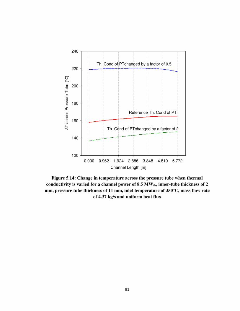
81

0.000 0.962 1.924 2.886 3.848 4.810 5.772

∆T

acro

ss P

ressu

re T

ube

[°C

]

120

140

160

180

200

220

240

Channel Length [m]

Reference Th. Cond of PT

Th. Cond of PTchanged by a factor of 0.5

Th. Cond of PTchanged by a factor of 2

Figure 5.14: Change in temperature across the pressure tube when thermal

conductivity is varied for a channel power of 8.5 MWth, inner-tube thickness of 2

mm, pressure tube thickness of 11 mm, inlet temperature of 350°C, mass flow rate

of 4.37 kg/s and uniform heat flux

82

In summary, the total heat loss to moderator when no insulation is used is much higher

compared to the reference HEC and current CANDU-6 fuel-channels [45]. Placing a

ceramic used in the HEC channel outside the pressure tube in the Re-Entrant should

reduce heat loss in the Re-Entrant channel. A solid moderator could also be used to

address boiling concerns. The following section examines the heat loss for an insulated

Re-Entrant fuel-channel.

5.2.2 Porous Yttria Stabilized Zirconia Insulated Re-Entrant Channel

Porous Yttria Stabilized Zirconia (YSZ) with 70% porosity has been chosen as one

insulating option for the Re-Entrant channel as zirconia is exceptionally resistant to

irradiation damage from fast neutrons and energetic ions [9]. Figure 3.5 shows the

insulator in the Re-Entrant fuel-channel. The pores in the insulator are in the axial

direction along the fuel-channel. This allows for carbon dioxide gas to pass through them.

The reference thickness of the insulator is 7 mm as an analysis on the insulator thickness

indicated that the minimum thickness of the insulator required to prevent boiling of the

moderator is 6 mm.

Figure 5.15 shows the temperature profiles of the coolant, the inner and outer surfaces of

the flow, pressure and outer tubes, and the outer sheath along the heated length of the

channel for a channel power of 8.5 MWth, an inner-tube thickness of 2 mm, a pressure

tube thickness of 11 mm, and a 7 mm thick porous YSZ insulator. The temperature of the

outer sheath is lowest at the pseudocritical point, which can be seen in Figure 5.15. The

outer tube temperature indicates that boiling does not occur in the moderator. The exit

temperature of the hot side is 610°C, which is considerably higher than the Re-Entrant

model with no insulation (560°C). This indicates that the insulator is reducing the

thermal energy transferred to the moderator.

83

The temperature gradients across the radial section of the Porous YSZ insulated Re-

Entrant fuel-channel at x = 0 m, x = 1.44 m and x = 5.772 m are shown in Figure 5.16,

where x = 1.44 m is the location of the pseudocritical point. The dotted line indicates the

expected temperature profile in the liquid. As mentioned earlier, the temperature

difference between the outer tube and the moderator indicates that boiling of the

moderator does not occur. The thermophysical properties for the 7 mm thick porous YSZ

insulated REC are shown in Appendix C.

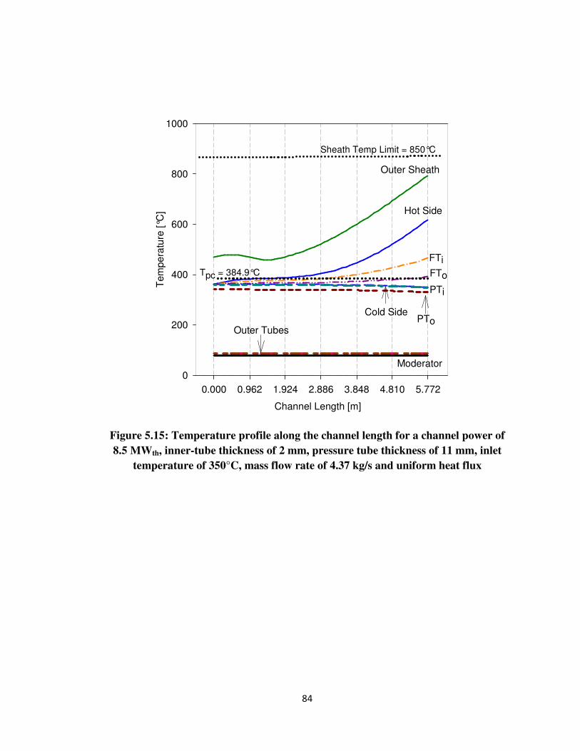
84

Channel Length [m]

0.000 0.962 1.924 2.886 3.848 4.810 5.772

Tem

pe

ratu

re [°C

]

0

200

400

600

800

1000

Tpc = 384.9°C


Moderator

Outer Sheath

Hot Side

PTo

PTi

FTi

FTo

Cold Side

Outer Tubes

Figure 5.15: Temperature profile along the channel length for a channel power of



85


50 60 70 80 90 100

Te

mpe

ratu

re [°C

]

0

100

200

300

400

500

600

Moderator



Pressure Tube Inner SurfacePressure Tube Outer Surface

Outer Tube Outer Surface

Outer Tube Inner Surface


Porous YSZ insulated Re-Entrant channel

x = 5.772 m


x = 0 m

86

5.2.3 Zirconium Dioxide (ZrO2) Insulated Re-Entrant Channel

Another insulating option for the Re-Entrant channel is to use a solid Zirconium Dioxide

insulation. The minimum thickness required to prevent boiling of the moderator is 5 mm.

The reference thickness chosen for this analysis is 7 mm, so that the results can be

compared to the Re-Entrant channel with Porous Yttria Stabilized Zirconia insulation.

Heat transfer analysis was also performed for a 7 mm solid ZrO2 insulated fuel-channel.

The reference thermal conductivity of zirconium dioxide is 2.7 �/� ∙ #. [9]. The

temperature profiles are shown in Figure 5.17, while thermophysical properties are shown

in Appendix C. The outer temperature profile of the pressure tube in the solid zirconium

dioxide channel is lower than the outer temperature profile in the YSZ insulated channel.

This indicates that more heat is being lost from the cold side to the moderator in the

zirconium dioxide insulated channel. The thermophysical properties profiles are similar

between the two cases as the pseudocritical points are relatively close to each other.

The temperature gradients across the radial section of the reference Re-Entrant fuel-

channel at x = 0 m, x = 1.54 m, and x = 5.772 m, are shown in Figure 5.18, where

x = 1.54 m is the location of the pseudocritical point. The dotted line indicates the

expected temperature profile in the liquid. The heavy water moderator does not boil

boiling of the moderator does not for the ZrO2 fuel-channel occur.

87

Channel Length [m]

0.000 0.962 1.924 2.886 3.848 4.810 5.772

Te

mp

era

ture

[°C

]

0

200

400

600

800

1000

Tpc = 384.9°C


Moderator

Outer Sheath

Hot Side

PTo

PTi

FTi

FTo

Cold Side

Outer Tubes

Figure 5.17: Temperature profile along the ZrO2 insulated channel length for a

channel power of 8.5 MWth, inner-tube thickness of 2 mm, pressure tube thickness

of 11 mm, insulation thickness of 7 mm, inlet temperature of 350°C, mass flow rate

of 4.37 kg/s and uniform heat flux

88


50 60 70 80 90 100

Te

mpe

ratu

re [°C

]

0

100

200

300

400

500

600

Moderator



Pressure Tube Inner Surface

Pressure Tube Outer Surface

Outer Tube Outer Surface

Outer Tube Inner Surface


ZrO2 insulated Re-Entrant channel for a channel power of 8.5 MWth, inner-tube

thickness of 2 mm, pressure tube thickness of 11 mm, insulation thickness of 7 mm,


x = 5.772 m


x = 0 m

89

5.2.4 Heat Loss Comparison

When the reactor is under normal operation, heat loss from the channel to the moderator

is assumed to be via mixed forced and free convection. This is because the Rayleigh

number from free convection is high enough, that the thermal buoyancy cannot be

ignored. Heat transfer to the moderator will occur via free convection during accident

scenarios such as failure of moderator pumps. The total heat loss to the moderator from

the Re-Entrant channel for both the Porous YSZ insulation and the ZrO2 insulation when

insulation thickness is varied is shown Figure 5.19 for mixed type heat loss and Figure

5.20 for free convection heat loss. The total heat loss to the moderator is much lower

when the Porous YSZ insulation is used for both types of heat loss. One advantage of

using solid ZrO2 is that there is no need for an additional system for the gas that would

flow through the Porous YSZ insulation. However, the CO2 gas that flows through the

insulator has other advantages such as the ability to detect leaks in the pressure tube.

Thus, Porous YSZ is chosen as the insulator for the Re-Entrant fuel-channel.

A comparison between the total heat loss for a 7 mm Porous YSZ insulated channel, 7

mm ZrO2 insulated channel, reference HEC SCWR fuel-channel, and the CANDU-6 fuel-

channel is shown in Table 5.2. The heat loss from the CANDU-6 channel has been

scaled to match the channel power of the Re-Entrant channel. The total heat loss in the 7

mm Porous YSZ insulation is about 1.02% of the channel’s total power.

90

6 7 8 9 10 11 12

He

at L

oss to M

od

era

tor

[kW

]

0

50

100

150

200

250

300

Insulation Thickness [mm]

Solid ZrO2

Porous YSZ

Mixed Type Flow

Figure 5.19: Heat loss to Moderator for cold side of Re-Entrant channel for variable

Porous YSZ insulation thickness and variable solid ZrO2 insulation thickness

assuming mixed type heat loss to the moderator

91

6 7 8 9 10 11 12

He

at Lo

ss to M

od

era

tor

[kW

]

0

50

100

150

200

250

300

Insulation Thickness [mm]

Solid ZrO2

Porous YSZ

Free Convection

Figure 5.20: Heat loss to Moderator for cold side of Re-Entrant channel for variable

Porous YSZ insulation thickness and variable solid ZrO2 insulation thickness

assuming free convection heat loss to the moderator

92

Table 5.2: Heat Loss Comparison for insulated Re-Entrant channel

Total Heat Loss

Per Channel

(kW)

Total Heat Loss in Reactor

(MW)

Re-Entrant Channel with 7 mm

Porous YSZ insulation (Mixed

Flow)

85 25.5 MW (300 channels)


ZrO2 insulation

(Mixed Flow)

225 67.5 MW (300 channels)


Porous YSZ insulation (Free

Convection Heat Loss)

80 24 MW (300 channels)


ZrO2 insulation

(Free Convection Heat Loss)

212 63.3 MW (300 channels)

Reference HEC SCWR Fuel-

Channel Concept 104 31.2 MW (300 channels)

CANDU-6 Fuel Channel (scaled

to 8.5 MWth channel power

equivalent)

13 5 MW (380 channels)

In summary, the heat loss from the Re-Entrant channel is greatly reduced when an

insulator is used. Two different insulators, Porous YSZ and solid ZrO2 were used and the

total heat loss was less for the Porous YSZ insulation for both free convection heat loss to

moderator the mixed type flow heat loss to the moderator.

93

5.3 Impact of Non-Uniform Flux Shapes

For the previous analyses, the heat flux in the fuel-channel was assumed to be uniform.

In this section, the heat loss to the moderator is examined for six different axial power

profiles:

• Case 1: Uniform axial power profile (reference)

• Case 2: Typical nominal axial power profile

• Case 3: Peaked shaped axial power profile

• Case 4: Upstream-skewed axial power profile

• Case 5: Downstream-skewed axial power profile

• Case 6: Variable axial power profile

Case 1 is used since the majority of experimental data available for determining heat

transfer models use a uniform heat flux. Hence the profile can be used for verification

against experimental data.

Case 2 represents a standard case for normal operating conditions in a nuclear reactor.

The flux shape is a slightly flattened cosine which occurs due to neutron leakage at the

boundary of the reactor. The slight flattening of the cosine shape is caused by internal

reactivity mechanisms such as adjuster rods or zone controls.

Case 3 is similar to Case 2, but represents a more severe gradient in the flux shape as

there is no flattening effect by the reactivity mechanisms.

Case 4 is the inverse of Case 5. Case 5 is a designed flux shape that envelopes several

refuelling scenarios in such a way as to be the most severe flux shape in critical heat flux

studies. Hence, recent experimental data was obtained using these flux shapes.

The first 5 cases are typically used in research related analysis as they are usually

sufficient to capture the phenomena for existing plants. In actual safety analysis of a

94

CANDU-6, over 900 flux shapes representing different normal and abnormal operating

scenarios are used. As the reactor physics flux shapes for SCWRs are not known, one

additional case is added for interest.

Case 6 is a disturbed flux shape usually caused by a reactivity device that is an outof-

normal configuration. The result is a two-peak flux shape. This slope was chosen as it

implies the possibilities of having the pseudocritical point in two locations or extended

over a region and hence could represent a scenario of significant safety concern.

Once the reactor physics flux shapes for SCWRs are known, the choice of flux shapes

can be revisited.

A 7 mm thick Porous YSZ insulated channel was used to analyze the impact of non-

uniform flux shapes. The total channel power was assumed to be 8.5 MWth for all cases,

while the inlet temperature was 350°C and mass flow rate was 4.37 kg/s. Heat loss to the

moderator was assumed to be via mixed flow.

The various axial power profiles are shown in Figures 5.21. The corresponding

temperature profiles are shown in Figures 5.22 to 5.27. The thermophysical properties

are shown in Appendix C for Case 1 and in Appendix D for Case 2 to 6.

The temperature profiles for all the five different axial power profiles indicate that the

coolant outlet temperature is approximately 600°C which is close to the desired value of

625°C. The outer sheath temperature is below the sheath temperature limit of 850°C for

all five different flux shapes, although it is close to the sheath limit for the down-skew

power profile.

95

Channel Length [m]

0.000 0.962 1.924 2.886 3.848 4.810 5.772

Po

we

r [k

W]

0

200

400

600

800

1000

1200

Case 1: Uniform axial power profile

Case 2: Typical nominal axial power profile

Case 3: Peaked shaped axial power profile

Case 4: Upstream-skewed axial power profile

Case 5: Downstream-skewed axial power profile

Case 6: Variable axial power profile

Figure 5.21: Axial Power Profiles

96

Channel Length [m]

0.000 0.962 1.924 2.886 3.848 4.810 5.772

Tem

pe

ratu

re [°C

]

0

200

400

600

800

1000

Tpc = 384.9°C


Moderator

Outer Sheath

Hot Side

PTo

PTi

FTi

FTo

Cold Side

Outer Tubes

Figure 5.22: Case 1 (Uniform Power Profile): Temperature profiles along the 7 mm

thick Porous YSZ insulated fuel-channel for a total channel power of 8.5 MWth,

inner-tube thickness of 2 mm, pressure tube thickness of 11 mm, inlet temperature

of 350°C and mass flow rate of 4.37 kg/s

97

Channel Length [m]

0.000 0.962 1.924 2.886 3.848 4.810 5.772

Tem

pe

ratu

re [°C

]

0

200

400

600

800

1000

Tpc = 384.9°C


Moderator

Outer Sheath

Hot Side

PTo

PTi

FTi

FTo

Cold SideOuter Tubes

Figure 5.23: Case 2 (Typical Nominal Power Profile): Temperature profiles along

the 7 mm thick Porous YSZ insulated fuel-channel for a total channel power of 8.5



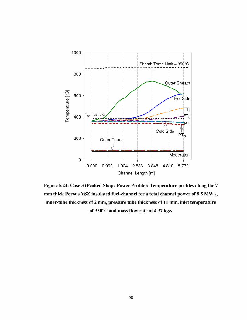
98

Channel Length [m]

0.000 0.962 1.924 2.886 3.848 4.810 5.772

Te

mp

era

ture

[°C

]

0

200

400

600

800

1000

Tpc = 384.9°C


Moderator

Outer Sheath

Hot Side

PTo

PTi

FTi

FTo

Cold Side

Outer Tubes

Figure 5.24: Case 3 (Peaked Shape Power Profile): Temperature profiles along the 7

mm thick Porous YSZ insulated fuel-channel for a total channel power of 8.5 MWth,



99

Channel Length [m]

0.000 0.962 1.924 2.886 3.848 4.810 5.772

Tem

pe

ratu

re [°C

]

0

200

400

600

800

1000

Tpc = 384.9°C


Moderator

Outer Sheath

Hot Side

PTo

PTi

FTi

FTo

Cold Side

Outer Tubes

Figure 5.25: Case 4 (Upstream-skewed Power Profile): Temperature profiles along

the 7 mm thick Porous YSZ insulated fuel-channel for a total channel power of 8.5



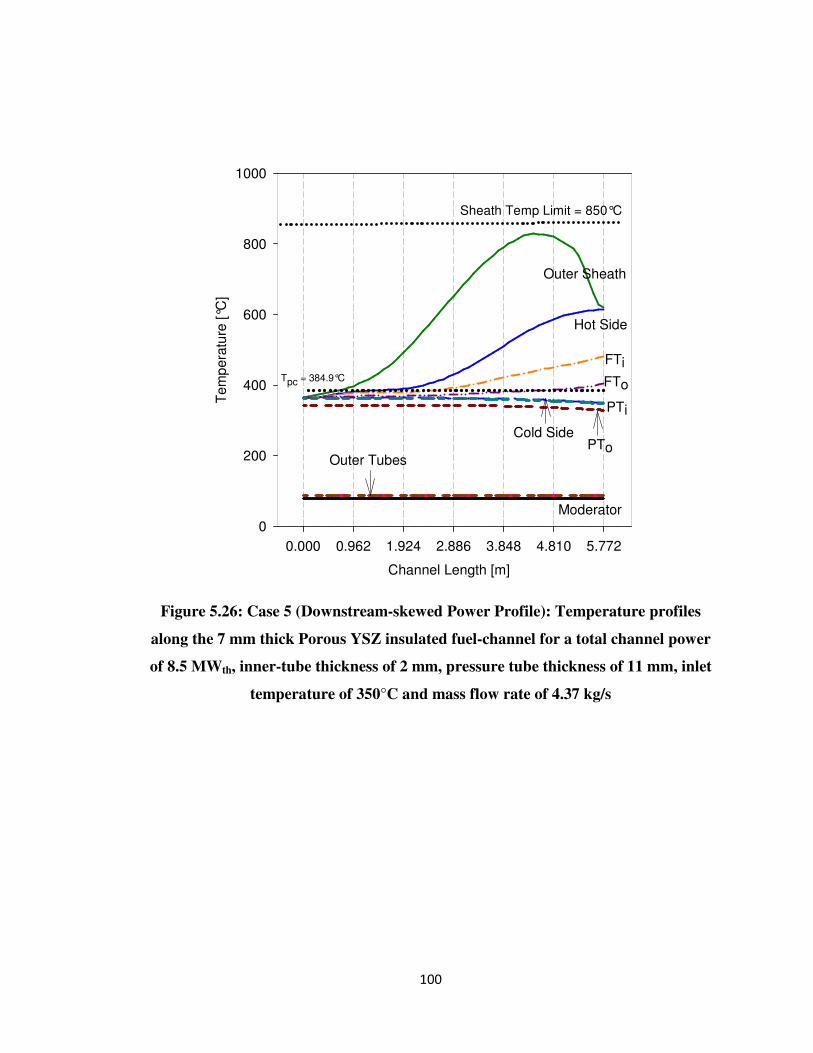
100

Channel Length [m]

0.000 0.962 1.924 2.886 3.848 4.810 5.772

Te

mp

era

ture

[°C

]

0

200

400

600

800

1000

Tpc = 384.9°C


Moderator

Outer Sheath

Hot Side

PTo

PTi

FTi

FTo

Cold Side

Outer Tubes

Figure 5.26: Case 5 (Downstream-skewed Power Profile): Temperature profiles

along the 7 mm thick Porous YSZ insulated fuel-channel for a total channel power

of 8.5 MWth, inner-tube thickness of 2 mm, pressure tube thickness of 11 mm, inlet


101

Channel Length [m]

0.000 0.962 1.924 2.886 3.848 4.810 5.772

Te

mp

era

ture

[°C

]

0

200

400

600

800

1000

Tpc = 384.9°C


Moderator

Outer Sheath

Hot Side

PTo

PTi

FTi

FTo

Cold Side

Outer Tubes

Figure 5.27: Case 6 (Variable Power Profile): Temperature profiles along the 7 mm

thick Porous YSZ insulated fuel-channel for a total channel power of 8.5 MWth,



102

The total heat loss from the reference 7 mm thick Porous YSZ insulated Re-Entrant

channel for the five different axial heat flux profiles is shown in Table 5.3. As expected,

the total heat loss is similar in all five cases as the total channel power is 8.5 MWth.

Table 5.4 shows the peak sheath temperature and its axial location in the Re-Entrant fuel-

channel for the six different cases. The peak sheath temperature of the downstream-

skewed profile is close to the sheath temperature limit which is 850°C. This maybe an

issue when the reactor is in operation as there are several hundred possible power

profiles, and power profiles similar to the downstream-skewed profile used in this

analysis may cause the sheath temperature to exceed the limit.

The location of the pseudocritical point for all six cases is shown in Table 5.5. The

pseudocritical point is located in bundle #3 for the uniform power profile, the typical

nominal power profile and the two peak power profile and in bundle #4 for the peaked

shape power profile. As expected, the pseudocritical point for the upstream-skewed

power profile occurs before the other cases, in bundle #2, while the pseudocritical point

for the downstream-skewed power profile occurs in bundle #5. The location of the

pseudocritical point for different power profiles in the Re-Entrant channel is important

because it affects the thermophysical properties, which in turn affects the heat transfer

characteristics of the fuel-channel.

103

Table 5.3: Heat Loss Comparison for insulated Re-Entrant channel with different


Power Profile Total Heat Loss Per

Channel (kW)

Case 1: Uniform power profile 84.52

Case 2: Typical nominal power profile 84.73

Case 3: Peaked shaped power profile 85.11

Case 4: Upstream-skewed power profile 85.41

Case 5: Downstream-skewed power profile 84.53

Case 6: Two peak power profile 84.73

104

Table 5.4: Peak sheath temperature and location of peak sheath temperature for

insulated Re-Entrant channel with different axial power profiles

Power Profile Peak Sheath

Temperature

(°C)

Location of Peak

Sheath Temp

(m)

Case 1: Uniform power profile 768.3 5.772

Case 2: Typical nominal power profile 688.1 4.81

Case 3: Peaked shaped power profile 733.2 3.85

Case 4: Upstream-skewed power profile 752.1 1.44

Case 5: Downstream-skewed power profile 829.4 4.43

Case 6: Two peak power profile 663.1 4.81

105

Table 5.5: Location of pseudocritical point in the Re-Entrant channel with different


Power Profile Location of pc

point (m)

Case 1: Uniform power profile 1.54

Case 2: Typical nominal power profile 1.83

Case 3: Peaked shaped power profile 2.02

Case 4: Upstream-skewed power profile 1.35

Case 5: Downstream-skewed power profile 2.50

Case 6: Two peak power profile 1.64

106

CHAPTER 6

CONCLUDING REMARKS

An alternate fuel-channel concept called the Re-Entrant Channel for SuperCritical Water-

cooled Reactors was conceptually designed and a preliminary heat transfer analysis was

performed to assess the thermal hydraulic behaviour under normal operating conditions.

• The temperature profiles of the coolant, outer sheath, inner and outer surfaces of

the flow tube, pressure tube and the outer tube were estimated at different

operating conditions. The temperature profiles of the coolant in the hot side and

of the outer sheath change considerably within the pseudocritical region. The

outer sheath temperature was below the sheath temperature limit for normal

operating conditions.

• The pseudocritical point was located in the hot side of the Re-Entrant fuel-channel

for various power profiles. The location of the pseudocritical point changes for

different axial power profiles and is important as it affects the heat transfer

characteristics and may affect the materials and chemistry characteristics of the

Re-Entrant channel.

• The cold side (annulus) acts as a preheater and recovers some of the heat lost.

The preheating concept also allowed for the pseudocritical point to be upstream of

the fuelled length.

• The Re-Entrant channel can be used in both horizontal and vertical configurations

and the design allowed for the insulator to be placed outside of the fuel-channel.

• Various axial power profiles did not have a significant impact on the total heat

loss to the moderator.

107

• Porous Yttria Stabilized Zirconia is found to be a more effective insulator than

Zirconium dioxide in terms of heat loss for the Re-Entrant channel.

• The total heat loss to the moderator for the porous Yttria Stabilized Zirconia

insulated Re-Entrant channel is 85 kW per channel for a channel power of 8.5

MWth, which is approximately 1% of the channel’s total power, and is 18% less

than the heat loss in the existing SCWR channel-type design concept. Thus, the

Re-Entrant channel is more efficient than the High Efficiency Channel in terms of

total heat loss to the moderator.

108

CHAPTER 7

FUTURE WORK

Future work should include optimizing the design of the Re-Entrant fuel-channel to

further reduce the heat loss from the cold side to the moderator and to see if it’s possible

to move the location of the pseudocritical point from the hot side to the cold side of the

fuel-channel.

A 2-D model of the re-entrant zone should be developed to investigate heat transfer

characteristics of the mixing node.

The use of a gaseous insulation similar to that used in the present CANDUs should also

be investigated as this may reduce heat loss. The effect of increasing the temperature and

pressure of the heavy water moderator on the minimum thickness of the insulator

required to prevent boiling should be studied as this will lead to a thinner insulator for the

fuel-channel design.

Using different solid and liquid moderators should also be considered as this may

eliminate the need for an insulator.

A detailed sensitivity analysis on the materials used for the flow and pressure tubes

should be conducted as data on how the metals perform at supercritical pressures and

temperatures becomes available.

The support structure for the flow and pressure tubes should be designed and the pressure

drop along the fuel-channel should be added to the heat transfer model as it may impact

the thermophysical properties of the coolant.

Changing operating conditions, such as mass flow and inlet temperatures, to account for

accident scenarios would also be useful.

109

REFERENCES

[1] I Hore-Lacy, Nuclear Energy in the 21st Century. London: World Nuclear University Press,

2006.

[2] Organisation for Economic Co-Operation and Development / International Energy Agency,

"World Enery Outlook," Paris, 2004.

[3] Ontario Power Generation. (2007, May) Energy Today Magazine. [Online].

http://www.energytodaymagazine.com/index.php?option=com_content&task=view&id=5750

[4] The International Association for the Properties of Water and Steam, "IAPWS Release on the

Values of Temperature, Pressure and Density of Ordinary Water Substances at their

Respective Critical Points," St. Petersburg, Russia, 1983.

[5] I. L. Pioro and R.B. Duffey, Heat Transfer and Hydraulic Resistance at Supercritical

Pressures in Power Engineering Applications. New York: ASME Press, 2007.

[6] C. K. Chow, S. J. Bushby, and H. F. Khartabil, "A Fuel Channel Design for CANDU-

SCWR," in 14th International Conference on Nuclear Engineering (ICONE14), Miami,

2006, pp. 677-685.

[7] I. L. Pioro, H. F. Khartabil, and R. B. Duffey, "Heat Transfer of Supercritical Fluids Flowing

in Channels - Emperical Correlations (Survey)," Nuclear Engineering and Design, vol. 230

(1-3), pp. 69-91, 2004.

[8] S. Mokry, "Development of a Heat-Transfer Correlation for Supercritical Water in

Supercritical Water-Cooled Reactor Applications," UOIT, Oshawa, Canada, 2009.

[9] C. K. Chow and H. F. Khartabil, "Conceptual Fuel Channel Designs for CANDU-SCWR,"

Nuclear Engineering and Technology, vol. 40 (1), 2008.

[10] G.L Brooks, "A Short History of the CANDU Nuclear Power System," 2002.

[11] AECL, "C-6 Technical Summary," Mississauga, Canada, 2005.

[12] AECL, "Enhanced CANDU 6 Technical Summary," Mississauga, Canada, 2009.

[13] AECL, "ACR-1000 Technical Summary," Mississauga, Canada, 2007.

[14] AECL, "CANDU: The Evolution," Nuclear Engineering International (NEI), 2007.

110

[15] GEN IV International Forum, "GIF R&D Outlook for Generation IV Nuclear Energy

Systems," 2007.

[16] U.S. DOE Nuclear Energy Research Advisory Committee and Generation IV International

Forum, "A Technology Roadmap for Generation IV Nuclear Energy Systems," 2002.

[17] D. Hahn et al., "Conceptual Design of the Sodium-Cooled Fast Reactor Kalimer-600," Korea

Atomic Energy Research Institution, Daejeon, 2007.

[18] JC Garnier, F, Morin, J. Y. Malo, and Y. Lejeail, "GFR System: Progress of CEA pre-

conceptual design studies," in International Congress on Advances in Nuclear Power Plants

(ICAPP 05), Seoul, 2005, p. 5305.

[19] L. Mathieu et al., "The thorium molten salt reactor: Moving on from the MSBR," Progress in

Nuclear Energy, vol. 48, no. 7, pp. 664-679, September 2006.

[20] L. Cinnoti et al., "The Potential of LFR and ELSY Project," in International Congress on

Advances in Nuclear Power Plants (ICAPP), Nice, 2007, p. 7585.

[21] Y. Oka and S. Koshizuka, "Coceptual design study of advanced power reactors," Progress in

Nuclear Energy, vol. 32, no. 1-2, pp. 167-177, 1998.

[22] H. Thind, I. Pioro, and G. Harvel, "SuperCritical Water-Cooled Nuclear Reactor with

Intermediate Heat Exchanges ," in 18th International Conference on Nuclear Engineering,

Xi'an, 2010, p. 30104.

[23] R. Monichan, "Steam Re-Heat Options for Supercritical Water Reactors," UOIT, Oshawa,

Canada, 2009.

[24] M Naidin, I Pioro, U Zirn, S Mokry, and G Naterer, "Supercritical Water-Cooled NPPs with

Co-Generation of Hydrogen: General Layout and Thermodynamic-Cycles Options," in The

4th International Symposium on Supercritical Water-Cooled Reactors, Heidelberg, Germany,

2009.

[25] B. V. Dyadyakin and A. S. Popov, "Heat Transfer and thermal resistance of tight seven-rod

bundle, cooled with water flow at supercritical pressures," Transactions of VTI, vol. 11, pp.

244 - 253, 1977.

[26] W.H. McAdams, Heat Transmission, 2nd ed. New York, USA: McGraw-Hill, 1942.

111

[27] N. M. Schnurr, V. S. Sastry, and A. B. Shapiro, "A numerical analysis of heat transfer to

fluids near the thermodynamic critical point including the thermal entrance region," Journal

of Heat Transfer, vol. 98 (4), pp. 609 - 615, 1976.

[28] F. Incropera, D. DeWitt, T. Bergman, and A. Lavine, Fundamentals of Heat and Mass

Transfer.: Wiley, 2006.

[29] A.A. Bishop, R.O. Sandberg, and L.S. Tong, "Forced convection heat transfer to water at

near-critical temperatures and super-critcial pressures," Atomic Power Division,

Westinghouse Electric Corporation, Pittsburgh, USA, 1964.

[30] H.S. Swenson, J.R. Carver, and C.R. Kakarala, "Heat transfer to supercritical water in

smooth-bore tubes," Journal of Heat Transfer, vol. 87 (4), 1965.

[31] P. Kirillov et al., "Experimental Study on Heat Transfer to Supercritical Water Flowing in

Vertical Tubes," in GLOBAL 2005 International Conference, Nuclear Energy Systems for

Future Generation and Global Sustainability (GLOBAL '05), Tsukuba, 2005.

[32] H. Zahlan, D.C. Groeneveld, and S. Tavoularis, "Look-up Table for Trans-Critical Heat

Transfer," in The 2nd Canada-China Joint Workshop on Supercritical Water Cooled

Reactors (CCSC 2010), Toronto, 2010.

[33] Y. M. Kim and H. J. Kim, "Analysis of fluid flow and heat transfer inside Calandria vessel of

CANDU-6 reactor using CFD," Nuclear Engineering and Technology , vol. 37 (6), pp. 575 -

586, 2005.

[34] L. Leung, "Effect of CANDU Bundle-Geometry Variation on Dryout Power," in 16th

International Conference on Nuclear Engineering, Florida, 2008, p. 48827.

[35] S. Hebert, "Identification and leaching of defective low void reactivity fuel," Royal Military

College of Canada, Kingston, MR52302, 2009.

[36] AK Steel, Product Data Bulletin - 304/304L Stainless Steel, 2007.

[37] B. Savioni, D. Caceres, I Vergara, R. Gonzalez, and J. Santiuste, "Radiation damage in

Neutron Irradiated Yttria-Stabilized-Zirconia Single Crystals," Journal of Nuclear Materials,

vol. 227, pp. 199-203, 2000.

[38] J. Holman, Heat Transfer, 9th ed. New York: McGrawHill, 2002.

[39] Y. Cengel and A. Ghajar, Heat and Mass Transfer, 4th ed. New York: McGraw Hill, 2010.

112

[40] J. Sweet, E. Roth, and M Moss, "Thermal Conductivity of Inconel 718 and Stainless Steel,"

International Journal of Thermophysics, 1987.

[41] E. Ruckestein and R. Rajagopalan, "A Simple Algebraic Method for Obtaining the Heat or

Mass Transfer Coefficients Under Mixed Convection," Chemical Engineering

Communications, 1980.

[42] S.W. Churchill and M. Bernstein, "A Correlating Equation for Forced Convection from

Gases and Liquids to a Circular Cylinder in Crossflow," Journal of Heat Transfer, vol. 19,

pp. 300 - 306, 1977.

[43] S.W. Churchill and H.H.S Chu, "Correlating Equations for Laminar and Turbulent Free

Convection from a Horizontal Cylinder," International Journal of Heat & Mass Transfer,

vol. 18, p. 1049.

[44] M. Kao, M. Lee, Y. Ferng, and C Chieng, "Heat transfer deterioration in a supercritical water

channel," Nuclear Engineering and Design, vol. 240, pp. 3321 - 3328, 2010.

[45] W. Peiman, E. Saltanov, K. Gabriel, and Pioro. I, "Heat Loss Calculations in a SCWR Fuel-

Channel," in 18th International Conference in Nuclear Engineering, Xi'an, China, 2010.

[46] L. Grande, "Thermal Aspects of Using Alternative Nuclear Fuels in Supercritical Water-

Cooled Reactors," UOIT, Oshawa, Canada, 2010.

113

APPENDIX A: NUMERICAL MODEL IN MATLAB

clear all;

clc

P=25000; % Pressure

mdot = 4.37; % Mass flow rate

d_bundle_centre = 18*10^-3; % Diameter of unheated fuel rod

d_bundle_elements = 11.5*10^-3; % Diameter of heated fuel rods

p_bundle = pi* 42*d_bundle_elements; % Perimeter of the bundle

A_bundle = (pi/4)*(1*d_bundle_centre^2+ 42*d_bundle_elements^2); % Cross Sectional Area of

bundle

di = 0.10345; % Inner diameter of inner(flow) tube

ri = di/2; % Inner radius of inner(flow) tube

do = di + 4*10^-3; % Outer diameter of inner(flow) tube

ro = do/2; % Outer radius of inner(flow) tube

Ac_flow_tube = (pi/4)*di^2; % Cross sectional area of flow tube

A_fl = Ac_flow_tube - A_bundle; % Flow Area of inner(flow) tube

p_wetted = pi*(42*d_bundle_elements + 1*d_bundle_centre + di); % Wetted perimeter of

inner(flow) tube

D_hy = 4*A_fl/p_wetted; % Hydraulic diameter of inner(flow) tube

G = mdot/A_fl; % Mass flux of inner(flow tube)

Di = sqrt((A_fl*4/pi)+do^2); % Inner d iameter of outer(pressure) tube

Ri = Di/2; % Inner radius of outer(pressure) tube

Do = Di + 14*10^-3; % Outer diameter of outer(pressure) tube

Ro = Do/2; % Outer radius of outer(pressure) tube

A_flow_annulus = (pi/4)*(Di^2 - do^2); % Flow area of annulus

D_hy_annulus = Di - do; % Flow area of annulus

G_annulus = mdot / A_flow_annulus; % Mass flow of annulus

% INSULATOR

d_ins_in = Do;

r_ins_in = d_ins_in/2;

thickness_ins = 7 ;

d_ins_out = d_ins_in + thickness_ins*2*10^-3;

r_ins_out = d_ins_out/2;

%OUTER TUBE

d_out_in = d_ins_out;

r_out_in = d_out_in/2;

thickness_out = 0.5;

d_out_out = d_out_in + thickness_out*2*10^-3;

r_out_out = d_out_out/2;

Q = 8.5*10^6; % Channel power

q = Q / (p_bundle*5.772); % Average heat flux of channel

nodes = 61; % Total nodes

114

n = nodes;

x= linspace(0,5.772,nodes);

for i = 1:(n-1);

X(i) = (x(i)+x(i+1))/2;

L(i) = x(i+1)-x(i);

end

L1 = [L,L(1)];

for i = 1:(n-1);

L2(i) = L1(i);

end

As_FT_i = pi * di * L; % Nodal inner surface area of inner(flow) tube

As_FT_o = pi * do * L; % Nodal outer surface area of inner(flow) tube

As_PT_i = pi * Di * L; % Nodal inner surface area of outer(pressure) tube

As_PT_o = pi * Do * L; % Nodal outer surface area of outer(pressure) tube

As_INS_i = pi* d_ins_in * L;

As_INS_o = pi* d_ins_out * L;

As_OUT_i = pi* d_out_in * L;

As_OUT_o = pi* d_out_out * L;

%***** Moderator

T_moderator = 80 + 273.15;

T_m = linspace(T_moderator,T_moderator,nodes-1);

pressure_m = 200; %101.3; % moderator pressure, kPa

g = 9.81;

T_inlet = 623.15; % Inlet temperature 350 C

Cp_cold_fluid_fluid(1) = refpropm('C','T',T_inlet,'P',P,'water'); % Cp from NIST

H_cold_fluid(1)= refpropm('H','T',T_inlet,'P',P,'water'); % Enthalpy from NIST

k_cold_fluid_fluid(1) = refpropm('L','T',T_inlet,'P',P,'water'); % Thermal Conductivity from NIST

mu_cold_fluid_fluid(1) = refpropm('V','T',T_inlet,'P',P,'water'); % Viscosity from NIST

T_cold_fluid = linspace(T_inlet,T_inlet+50,nodes+1); % Temperature profile for cold fluid

(estimate)

T_cold_initial_guess = T_cold_fluid - 273.15;

T_hot_fluid = linspace(898.15,T_cold_fluid(n+1),nodes+1); % Temperature profile for hot fluid

(estimate)

T_hot_initial_guess = T_hot_fluid - 273.15;

T_cold_fluid_actual(1) = T_inlet;

for i=1:n-1;

T_hot_fluid_bulk(i) = (T_hot_fluid(i) + T_hot_fluid(i+1))/2;

T_cold_fluid_bulk(i) = (T_cold_fluid(i) + T_cold_fluid(i+1))/2;

end;

115

for i=1:n-1;

T_FT_avg(i) = (T_hot_fluid_bulk(i)+T_cold_fluid_bulk(i))/2;

Ts_FT_i(i) = (T_hot_fluid_bulk(i) + T_FT_avg(i))/2; % Estimate for inner surface temp of flow tube

Ts_FT_o(i) = (T_cold_fluid_bulk(i) + T_FT_avg(i))/2;

T_INS_avg(i) = (T_cold_fluid_bulk(i)+ T_m(i))/2;

T_PT_avg(i) = (T_INS_avg(i)+ T_cold_fluid_bulk(i))/2;

Ts_PT_i(i) = (T_cold_fluid_bulk(i) + T_PT_avg(i))/2;

Ts_PT_o(i) = (T_PT_avg(i)+ T_INS_avg(i))/2;

T_OUT_avg(i) = (T_INS_avg(i)+ T_m(i))/2;

Ts_OUT_i(i) = (T_OUT_avg(i) + T_INS_avg(i))/2;

Ts_OUT_o(i) = (T_OUT_avg(i) + T_m(i))/2;

Ts_INS_i(i) = Ts_PT_o(i);

Ts_INS_o(i) = Ts_OUT_i(i);

end;

T_sheath = T_hot_fluid_bulk +300; % Initial guess for claddding temp

for i = 1:n-1; % Cladding temp calculations

delta_T = 4;

while (delta_T > 0.1)

H_w =refpropm('H','T',T_sheath(i),'P',P,'water');

H_b =refpropm('H','T',T_hot_fluid_bulk(i),'P',P,'water');

Cp = (H_w -H_b)/(T_sheath(i)-T_hot_fluid_bulk(i));

k =refpropm('L','T',T_hot_fluid_bulk(i),'P',P,'water');

mu = refpropm('V','T',T_hot_fluid_bulk(i),'P',P,'water');

Pr = (mu *Cp )/k;

rho_b = refpropm('D','T',T_hot_fluid_bulk(i),'P',P,'water');

rho_w = refpropm('D','T',T_sheath(i),'P',P,'water');

Re = G * D_hy / mu;

Nu = 0.0061 * Re^0.904 * Pr^0.684 * (rho_w/rho_b)^0.564;

h = Nu * k /D_hy;

T_sheath_new = (q/h)+T_hot_fluid_bulk(i);

delta_T = abs(T_sheath_new - T_sheath(i));

T_min = min(T_sheath(i),T_sheath_new);

T_sheath(i) = T_min +delta_T/2;

end

T_outer_sheath(i)= T_sheath(i);

rho_hot_fluid_b(i)= rho_b;

rho_hot_fluid_w(i)= rho_w;

Re_hot_fluid(i)= Re;

Nu_hot_fluid(i)= Nu;

Pr_hot_fluid(i)= Pr;

k_hot_fluid(i) = k;

h_hot_fluid(i)= h;

H_hot_fluid(i)= H_b;

end

T_hot_fluid_bulk_actual(1) = T_hot_fluid_bulk(1);

T_cold_fluid_bulk_actual(1) = T_cold_fluid_bulk(1);

116

trials = 1;

while(trials)<50

R_conv_1 = 1./ (h_hot_fluid .*As_FT_i); % Resistance of Hot fluid

for i=1:n-1;

T_FT_avg_r(i) = (Ts_FT_i(i) + Ts_FT_o(i))/2;

k_FT(i) =(2*10^(-6))*(T_FT_avg_r(i)^2) + 0.0134 * T_FT_avg_r(i) + 10.689; % Conductivity of

flow tube

R_cond_1(i) = (log(ro/ri))/(2*pi*L2(i)* k_FT(i)); % Resistance of flow tube

end

for i =1:n-1; % Cold fluid thermophysical properties

H_cold_fluid_w(i) = refpropm('H','T',Ts_FT_o(i),'P',P,'water');

H_cold_fluid_b(i) = refpropm('H','T',T_cold_fluid_bulk(i),'P',P,'water');

Cp_cold_fluid(i) = (H_cold_fluid_w(i) - H_cold_fluid_b(i))/(Ts_FT_o(i)-T_cold_fluid_bulk(i));

k_cold_fluid(i) = refpropm('L','T',T_cold_fluid_bulk(i),'P',P,'water');

mu_cold_fluid(i) = refpropm('V','T',T_cold_fluid_bulk(i),'P',P,'water');

Pr_cold_fluid(i) = (mu_cold_fluid(i) *Cp_cold_fluid(i))/k_cold_fluid(i);

rho_cold_fluid_b(i) = refpropm('D','T',T_cold_fluid_bulk(i),'P',P,'water');

rho_cold_fluid_w(i) = refpropm('D','T',Ts_FT_o(i),'P',P,'water');

Re_cold_fluid(i) = G_annulus * D_hy_annulus / mu_cold_fluid(i);

Nu_cold_fluid(i) = 0.0061 * Re_cold_fluid(i)^0.904 * Pr_cold_fluid(i)^0.684 *

(rho_cold_fluid_w(i)/rho_cold_fluid_b(i))^0.564;

h_cold_fluid(i) = Nu_cold_fluid(i) * k_cold_fluid(i) /D_hy_annulus;

end

R_conv_2 = 1./(h_cold_fluid .* As_PT_i); % Resistance of cold fluid

%******* PRESSURE TUBE

for i = 1:n-1;

T_PT_avg_r(i) = (Ts_PT_i(i) + Ts_PT_o(i))/2;

k_PT(i) =((2*10^(-6))*T_PT_avg_r(i)^2 + 0.0134* T_PT_avg_r(i) + 10.689);

R_cond_2(i) = (log(Ro/Ri))/(2 * pi * L2(i) * k_PT(i));

end

%********INSULATION

for i = 1:n-1;

T_INS_avg(i) = (Ts_INS_i(i) + Ts_INS_o(i))/ 2;

th_cond_air(i) = 8*10^(-5)*T_INS_avg(i) - 0.0072; %% CO2

k_INS(i) = 2.7 *0.3 + 0.7*th_cond_air(i) ; % Conductivity of insulation

R_cond_INS(i) = (log(r_ins_out/r_ins_in))/(2*pi*L2(i)*k_INS(i)); % Resistance of insulation

end

%********OUTER TUBE

for i=1:n-1;

T_OUT_avg_r(i) = (Ts_OUT_i(i) + Ts_OUT_o(i))/2;

k_OUT(i) =((2*10^(-6))*(T_OUT_avg_r(i))^2 + 0.0134 * T_OUT_avg_r(i) + 10.689);

R_cond_OUT(i) = (log(r_out_out/r_out_in))/(2 * pi * L2(i)* k_OUT(i));

117

end

%********MODERATOR

for i = 1:n-1;

T_m_PT_avg(i) = (T_m(i) + Ts_OUT_o(i))/2;

if (T_m_PT_avg(i)>394.55)

T_m_PT_avg(i) = 394.55;

end

beta_m(i) = 1 /T_m_PT_avg(i);

end

for i = 1:n-1;

density_m(i) = refpropm('D','T',T_m_PT_avg(i),'P',pressure_m,'D2O');

viscosity_m(i) = refpropm('V','T',T_m_PT_avg(i),'P',pressure_m,'D2O');

k_m(i) = refpropm('L','T',T_m_PT_avg(i),'P',pressure_m,'D2O');

Cp_m(i) = refpropm('C','T',T_m_PT_avg(i),'P',pressure_m,'D2O');

end

Pr_m = viscosity_m .* Cp_m ./k_m;

k_viscosity_m = viscosity_m ./ density_m;

% FREE CONVECTION

for i = 1:n-1;

if(Ts_OUT_o(i))<T_m(i)

Ts_OUT_o(i) = T_m(i);

end

Ra_m_D4(i) = (g * beta_m(i)*(Ts_OUT_o(i) - T_m(i))*d_out_out^3*

Pr_m(i))/((k_viscosity_m(i))^2);

Nu_m_D4_free(i) = (0.6 + (0.387 * Ra_m_D4(i)^(1/6))/(1 +

(0.559/Pr_m(i))^(9/16))^(8/27))^2;

end

% FORCED CONVECTION

for i = 1:n-1;

Re_m_D4(i) = (0.95*d_out_out)/k_viscosity_m(i); % v=0.018

Nu_m_D4_forced(i) = 0.3 +

((0.62*(Re_m_D4(i)^(1/2))*(Pr_m(i)^(1/3)))/((1+(0.4/(Pr_m(i)))^(2/3))^(1/4)))*(1+((Re_m_D

4(i)/282000)^(5/8)))^(4/5);

if (Re_m_D4(i)>20000 && Re_m_D4(i)<400000)

Nu_m_D4_forced(i) = 0.3 +

((0.62*(Re_m_D4(i)^(1/2))*(Pr_m(i)^(1/3)))/((1+(0.4/(Pr_m(i)))^(2/3))^(1/4)))*(1+((Re_m_D

4(i)/282000)^(1/2)));

end

end

118

Nu_m_D4 = (Nu_m_D4_free.^3 + Nu_m_D4_forced.^3).^(1/3);

h_m_D4 = k_m .* Nu_m_D4 ./ d_out_out;

R_m = 1 ./(h_m_D4 .* As_OUT_o);

R_mm = 1 ./(h_m_D4 .* pi * d_out_out);

MOD_HEAT_LOSS = h_m_D4.*(3.142.*d_out_out.*0.0962).*(Ts_OUT_o - T_m);

MOD_HEAT_LOSS_TOTAL = sum(MOD_HEAT_LOSS);

R_total = R_conv_1 + R_cond_1 + R_conv_2; % Total Resistance

UA = 1./ R_total; % UA

DeltaT = T_hot_fluid_bulk - T_cold_fluid_bulk;

Qdot = UA .* DeltaT;

Qdot_total = sum(Qdot);

%*******Heat Loss to Moderator

R_m_total = R_conv_2 + R_cond_2 + R_cond_INS + R_cond_OUT + R_m;

UA_m = (1./ R_m_total);

DeltaT_m = T_cold_fluid_bulk - T_m;

heat_loss_m = UA_m .* DeltaT_m;

heat_loss_m_total = sum(heat_loss_m);

qdot = Qdot ./ As_FT_i;

Qdot_net = Qdot - heat_loss_m;

for i=1:n-1; % Cold fluid end temp using Qdot

H_cold_fluid(i+1) = (H_cold_fluid(i)+ (Qdot_net(i)/mdot));

T_cold_fluid_actual(i+1) = refpropm('T','H',H_cold_fluid(i+1),'P',P,'water');

end

for i=1:n-1;

T_cold_fluid_bulk_actual(i) = (T_cold_fluid_actual(i) + T_cold_fluid_actual(i+1))/2;

end

Q_net = Q - Qdot_total; %Net Heat (Power - Total Heat loss)

q = Q_net/ (p_bundle*5.772); % Avg heat flux for hot side

%Variable Power Profile

bp = [182.13 420.71 561.36 600.54 664.07 713.65 713.56 663.83 583.41 518.38 377.96 165.55];

bp = [.21188E+03 .48466E+03 .63500E+03 .65889E+03 .70094E+03 .72986E+03

.72492E+03 .68886E+03 .62404E+03 .57426E+03 .42741E+03 .18914E+03 ];

bp = [.20216E+03 .48237E+03 .67457E+03 .77740E+03 .77341E+03 68315E+03 .45170E+03

.50743E+03 .60024E+03 .52531E+03 .37295E+03 .15740E+03];

119

bp = [.18057E+03 .43223E+03 .64382E+03 .85966E+03 .10684E+04 .10857E+04

.10855E+04 .10681E+04 .83568E+03 .59492E+03 .38855E+03 .16415E+03];

bp = [625 850 1010 1040 1000 950 850 775 625 475 175 125];

bp = [125 175 475 625 775 850 950 1000 1040 1010 850 625];

bp = [708.33 708.33 708.33 708.33 708.33 708.33 708.33 708.33 708.33 708.33 708.33 708.33];

bp(end:-1:1);

test_bp_total = sum(bp);

for k=1:11

avg(k) = (bp(k)+bp(k+1))/2;

bundlepower_old(k+1) = avg(k);

end

bundlepower_old(1) = 0;

bundlepower_old(13)= 0;

sum_bundlepower_old = sum(bundlepower_old);

diff_bundlepower_old = 8500 - sum_bundlepower_old;

add_bundlepower = diff_bundlepower_old/12;

bundlepower = bundlepower_old + add_bundlepower;

sum_bundlepower_new = sum(bundlepower);

y = bundlepower.*2.079;

% Node 1

a = 1;

b = 2;

i = 1;

j = 1;

while(a<13)

y1 = y(a);

y2 = y(b);

for mu = 0: 0.2: 1

val(i) = (y1*(1-mu)+y2*mu);

i = i+1;

end

for j=j:i-2;

nodalpower(j) = ((val(j)+val(j+1))/2)*0.0962;

end;

i = i - 1;

j = j + 1;

a = a + 1;

b = b + 1;

end

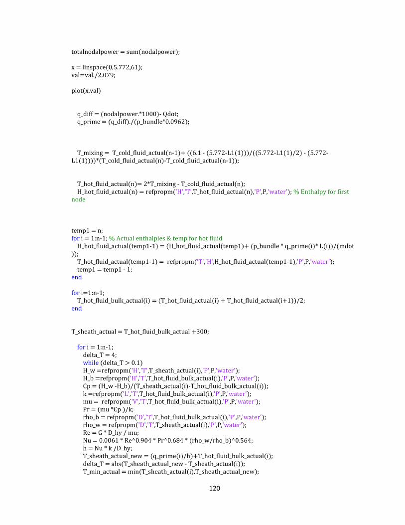
120

totalnodalpower = sum(nodalpower);

x = linspace(0,5.772,61);

val=val./2.079;

plot(x,val)

q_diff = (nodalpower.*1000)- Qdot;

q_prime = (q_diff)./(p_bundle*0.0962);

T_mixing = T_cold_fluid_actual(n-1)+ ((6.1 - (5.772-L1(1)))/((5.772-L1(1)/2) - (5.772-

L1(1))))*(T_cold_fluid_actual(n)-T_cold_fluid_actual(n-1));

T_hot_fluid_actual(n)= 2*T_mixing - T_cold_fluid_actual(n);

H_hot_fluid_actual(n) = refpropm('H','T',T_hot_fluid_actual(n),'P',P,'water'); % Enthalpy for first

node

temp1 = n;

for i = 1:n-1; % Actual enthalpies & temp for hot fluid

H_hot_fluid_actual(temp1-1) = (H_hot_fluid_actual(temp1)+ (p_bundle * q_prime(i)* L(i))/(mdot

));

T_hot_fluid_actual(temp1-1) = refpropm('T','H',H_hot_fluid_actual(temp1-1),'P',P,'water');

temp1 = temp1 - 1;

end

for i=1:n-1;

T_hot_fluid_bulk_actual(i) = (T_hot_fluid_actual(i) + T_hot_fluid_actual(i+1))/2;

end

T_sheath_actual = T_hot_fluid_bulk_actual +300;

for i = 1:n-1;

delta_T = 4;

while (delta_T > 0.1)

H_w =refpropm('H','T',T_sheath_actual(i),'P',P,'water');

H_b =refpropm('H','T',T_hot_fluid_bulk_actual(i),'P',P,'water');

Cp = (H_w -H_b)/(T_sheath_actual(i)-T_hot_fluid_bulk_actual(i));

k =refpropm('L','T',T_hot_fluid_bulk_actual(i),'P',P,'water');

mu = refpropm('V','T',T_hot_fluid_bulk_actual(i),'P',P,'water');

Pr = (mu *Cp )/k;

rho_b = refpropm('D','T',T_hot_fluid_bulk_actual(i),'P',P,'water');

rho_w = refpropm('D','T',T_sheath_actual(i),'P',P,'water');

Re = G * D_hy / mu;

Nu = 0.0061 * Re^0.904 * Pr^0.684 * (rho_w/rho_b)^0.564;

h = Nu * k /D_hy;

T_sheath_actual_new = (q_prime(i)/h)+T_hot_fluid_bulk_actual(i);

delta_T = abs(T_sheath_actual_new - T_sheath_actual(i));

T_min_actual = min(T_sheath_actual(i),T_sheath_actual_new);

121

T_sheath_actual(i) = T_min_actual +delta_T/2;

end

T_outer_sheath(i)= T_sheath_actual(i);

if T_outer_sheath(i)< T_hot_fluid_bulk_actual(i)

T_outer_sheath(i) = T_hot_fluid_bulk_actual(i);

end

h_hot_fluid(i)= h;

end

T_hot_fluid = T_hot_fluid_actual;

T_cold_fluid = T_cold_fluid_actual;

T_cold_fluid_bulk = T_cold_fluid_bulk_actual;

T_hot_fluid_bulk = T_hot_fluid_bulk_actual;

Ts_FT_i = T_hot_fluid_bulk - Qdot .* (R_conv_1);

Ts_FT_o = T_hot_fluid_bulk - Qdot .* (R_conv_1 + R_cond_1);

Ts_PT_i = T_cold_fluid_bulk - (heat_loss_m) .*(R_conv_2);

Ts_PT_o = T_cold_fluid_bulk - (heat_loss_m) .*(R_conv_2 + R_cond_2);

Ts_INS_i = Ts_PT_o;

Ts_INS_o = T_cold_fluid_bulk - (heat_loss_m) .*(R_conv_2 + R_cond_2 + R_cond_INS);

Ts_OUT_i = Ts_INS_o;

Ts_OUT_o = T_cold_fluid_bulk - (heat_loss_m) .*(R_conv_2 + R_cond_2 + R_cond_INS +

R_cond_OUT);

for i=1:n-1;

if(Ts_OUT_o(i)<T_m(i))

Ts_OUT_o(i) = T_m(i);

end

end

trials = trials + 1;

end

Ts_FT_end_avg = (T_hot_fluid(n)+T_cold_fluid(n))./2;

Ts_FT_i_plot(n) = (Ts_FT_end_avg+T_hot_fluid(n))./2;

Ts_FT_o_plot(n) = (Ts_FT_end_avg+T_cold_fluid(n))./2;

T_INS_end_avg = (T_cold_fluid(n)+ T_m(n-1))./2;

T_PT_end_avg = (T_INS_end_avg + T_cold_fluid(n))./2;

for i = 1:n-2;

Ts_FT_i_plot(i+1) = (Ts_FT_i(i) + Ts_FT_i(i+1))/2;

122

Ts_FT_o_plot(i+1) = (Ts_FT_o(i) + Ts_FT_o(i+1))/2;

end

Ts_FT_i_plot(1) = Ts_FT_i_plot(2)+ ((0 - L1(1))/(L1(1)/2 - L1(1)))*(Ts_FT_i(1)-Ts_FT_i_plot(2));

Ts_FT_o_plot(1) = Ts_FT_o_plot(2)+ ((0 - L1(1))/(L1(1)/2 - L1(1)))*(Ts_FT_o(1)-Ts_FT_o_plot(2));

for i = 1:n-2;

Ts_PT_i_plot(i+1) = (Ts_PT_i(i) + Ts_PT_i(i+1))/2;

Ts_PT_o_plot(i+1) = (Ts_PT_o(i) + Ts_PT_o(i+1))/2;

end

Ts_PT_i_plot(1) = Ts_PT_i_plot(2)+ ((0 - L1(1))/(L1(1)/2 - L1(1)))*(Ts_PT_i(1)-Ts_PT_i_plot(2));

Ts_PT_o_plot(1) = Ts_PT_o_plot(2)+ ((0 - L1(1))/(L1(1)/2 - L1(1)))*(Ts_PT_o(1)-

Ts_PT_o_plot(2));

for i = 1:n-2;

Ts_INS_i_plot(i+1) = (Ts_INS_i(i) + Ts_INS_i(i+1))/2;

Ts_INS_o_plot(i+1) = (Ts_INS_o(i) + Ts_INS_o(i+1))/2;

end

Ts_INS_i_plot(1) = Ts_INS_i_plot(2)+ ((0 - L1(1))/(L1(1)/2 - L1(1)))*(Ts_INS_i(1)-

Ts_INS_i_plot(2));

Ts_INS_o_plot(1) = Ts_INS_o_plot(2)+ ((0 - L1(1))/(L1(1)/2 - L1(1)))*(Ts_INS_o(1)-

Ts_INS_o_plot(2));

for i = 1:n-2;

Ts_OUT_i_plot(i+1) = (Ts_OUT_i(i) + Ts_OUT_i(i+1))/2;

Ts_OUT_o_plot(i+1) = (Ts_OUT_o(i) + Ts_OUT_o(i+1))/2;

end

Ts_OUT_i_plot(1) = Ts_OUT_i_plot(2)+ ((0 - L1(1))/(L1(1)/2 - L1(1)))*(Ts_OUT_i(1)-

Ts_OUT_i_plot(2));

Ts_OUT_o_plot(1) = Ts_OUT_o_plot(2)+ ((0 - L1(1))/(L1(1)/2 - L1(1)))*(Ts_OUT_o(1)-

Ts_OUT_o_plot(2));

Ts_PT_i_plot(n) = Ts_PT_i_plot(n-1);

Ts_PT_o_plot(n) = Ts_PT_o_plot(n-1);

Ts_OUT_i_plot(n) = Ts_OUT_i_plot(n-1);

Ts_OUT_o_plot(n) = Ts_OUT_o_plot(n-1);

Ts_INS_i_plot(n) = Ts_INS_i_plot(n-1);

Ts_INS_o_plot(n) = Ts_INS_o_plot(n-1);

for i = 1:n-2;

T_outer_sheath_plot(i+1) = (T_outer_sheath(i) + T_outer_sheath(i+1))/2;

if T_outer_sheath_plot(i+1)< T_hot_fluid_bulk_actual(i+1)

123

T_outer_sheath_plot(i+1) = T_hot_fluid_bulk_actual(i+1);

end

end

T_outer_sheath_plot(1) = T_outer_sheath_plot(2)+ ((0 - L1(1))/(L1(1)/2 -

L1(1)))*(T_outer_sheath(1)-T_outer_sheath_plot(2));

T_outer_sheath_plot(n) = T_outer_sheath_plot(n-1)+ ((5.772 - (5.772-L1(1)))/((5.772-L1(1)/2) -

(5.772-L1(1))))*(T_outer_sheath(n-1)-T_outer_sheath_plot(n-1));

for i = 1:n-2;

qdot_plot(i+1) = (qdot(i) + qdot(i+1))/2;

end

qdot_plot(1) = qdot_plot(2)+ ((0 - L1(1))/(L1(1)/2 - L1(1)))*(qdot(1)-qdot_plot(2));

qdot_plot(n) = qdot_plot(n-1)+ ((5.772 - (5.772-L1(1)))/((5.772-L1(1)/2) - (5.772-

L1(1))))*(qdot(n-1)-qdot_plot(n-1));

T_hot_fluid(n+1) = T_mixing;

T_cold_fluid(n+1) = T_mixing;

%Properties of hot fluid

for i=1:n-1;

H_hot_fluid_w_actual(i) = refpropm('H','T',T_outer_sheath(i),'P',P,'water');

H_hot_fluid_b_actual(i) = refpropm('H','T',T_hot_fluid_bulk(i),'P',P,'water');

Cp_hot_fluid_actual(i) = (H_hot_fluid_w_actual(i) - H_hot_fluid_b_actual(i))/(T_outer_sheath(i)-

T_hot_fluid_bulk(i));

k_hot_fluid_actual(i) = refpropm('L','T',T_hot_fluid_bulk(i),'P',P,'water');

mu_hot_fluid_actual(i) = refpropm('V','T',T_hot_fluid_bulk(i),'P',P,'water');

Pr_hot_fluid_actual(i) = (mu_hot_fluid_actual(i) *Cp_hot_fluid_actual(i))/k_hot_fluid_actual(i);

rho_hot_fluid_b_actual(i) = refpropm('D','T',T_hot_fluid_bulk(i),'P',P,'water');

rho_hot_fluid_w_actual(i) = refpropm('D','T',T_outer_sheath(i),'P',P,'water');

Re_hot_fluid_actual(i) = G * D_hy / mu_hot_fluid_actual(i);

Nu_hot_fluid_actual(i) = 0.0061 * Re_hot_fluid_actual(i)^0.904 * Pr_hot_fluid_actual(i)^0.684 *

(rho_hot_fluid_w_actual(i)/rho_hot_fluid_b_actual(i))^0.564;

h_hot_fluid_actual(i) = Nu_hot_fluid_actual(i) * k_hot_fluid_actual(i) /D_hy;

end

for i = 1:n-2;

H_hot_fluid_w_actual_plot(i+1) = (H_hot_fluid_w_actual(i)+ H_hot_fluid_w_actual(i+1))./2;

H_hot_fluid_b_actual_plot(i+1) = (H_hot_fluid_b_actual(i) + H_hot_fluid_b_actual(i+1))./2;

Cp_hot_fluid_actual_plot(i+1) = (Cp_hot_fluid_actual(i)+ Cp_hot_fluid_actual(i+1))./2;

k_hot_fluid_actual_plot(i+1) = (k_hot_fluid_actual(i) + k_hot_fluid_actual(i+1))./2;

mu_hot_fluid_actual_plot(i+1) = (mu_hot_fluid_actual(i) + mu_hot_fluid_actual(i+1))./2;

Pr_hot_fluid_actual_plot(i+1) = (Pr_hot_fluid_actual(i) + Pr_hot_fluid_actual(i+1))./2;

rho_hot_fluid_b_actual_plot(i+1) = (rho_hot_fluid_b_actual(i) + rho_hot_fluid_b_actual(i+1))./2;

rho_hot_fluid_w_actual_plot(i+1) = (rho_hot_fluid_w_actual(i) + rho_hot_fluid_w_actual(i+1))./2;

Re_hot_fluid_actual_plot(i+1) = (Re_hot_fluid_actual(i)+ Re_hot_fluid_actual(i+1))./2;

Nu_hot_fluid_actual_plot(i+1) = (Nu_hot_fluid_actual(i) + Nu_hot_fluid_actual(i+1))./2;

h_hot_fluid_actual_plot(i+1) = (h_hot_fluid_actual(i) + h_hot_fluid_actual(i+1))./2;

124

end

H_hot_fluid_w_actual_plot(1) = refpropm('H','T',T_outer_sheath_plot(1),'P',P,'water');

H_hot_fluid_b_actual_plot(1) = refpropm('H','T',T_hot_fluid(1),'P',P,'water');

Cp_hot_fluid_actual_plot(1) = (H_hot_fluid_w_actual_plot(1) -

H_hot_fluid_b_actual_plot(1))/(T_outer_sheath_plot(1)-T_hot_fluid(1));

k_hot_fluid_actual_plot(1) = refpropm('L','T',T_hot_fluid(1),'P',P,'water');

mu_hot_fluid_actual_plot(1) = refpropm('V','T',T_hot_fluid(1),'P',P,'water');

Pr_hot_fluid_actual_plot(1) = (mu_hot_fluid_actual_plot(1)

*Cp_hot_fluid_actual_plot(1))/k_hot_fluid_actual_plot(1);

rho_hot_fluid_b_actual_plot(1) = refpropm('D','T',T_hot_fluid(1),'P',P,'water');

rho_hot_fluid_w_actual_plot(1) = refpropm('D','T',T_outer_sheath_plot(1),'P',P,'water');

Re_hot_fluid_actual_plot(1) = G * D_hy / mu_hot_fluid_actual_plot(1);

Nu_hot_fluid_actual_plot(1) = 0.0061 * Re_hot_fluid_actual_plot(1)^0.904 *

Pr_hot_fluid_actual_plot(1)^0.684 *

(rho_hot_fluid_w_actual_plot(1)/rho_hot_fluid_b_actual_plot(1))^0.564;

h_hot_fluid_actual_plot(1) = Nu_hot_fluid_actual_plot(1) * k_hot_fluid_actual_plot(1) /D_hy;

H_hot_fluid_w_actual_plot(n) = refpropm('H','T',T_outer_sheath_plot(n),'P',P,'water');

H_hot_fluid_b_actual_plot(n) = refpropm('H','T',T_hot_fluid(n),'P',P,'water');

Cp_hot_fluid_actual_plot(n) = (H_hot_fluid_w_actual_plot(n) -

H_hot_fluid_b_actual_plot(n))/(T_outer_sheath_plot(n)-T_hot_fluid(n));

k_hot_fluid_actual_plot(n) = refpropm('L','T',T_hot_fluid(n),'P',P,'water');

mu_hot_fluid_actual_plot(n) = refpropm('V','T',T_hot_fluid(n),'P',P,'water');

Pr_hot_fluid_actual_plot(n) = (mu_hot_fluid_actual_plot(n)

*Cp_hot_fluid_actual_plot(n))/k_hot_fluid_actual_plot(n);

rho_hot_fluid_b_actual_plot(n) = refpropm('D','T',T_hot_fluid(n),'P',P,'water');

rho_hot_fluid_w_actual_plot(n) = refpropm('D','T',T_outer_sheath_plot(n),'P',P,'water');

Re_hot_fluid_actual_plot(n) = G * D_hy / mu_hot_fluid_actual_plot(n);

Nu_hot_fluid_actual_plot(n) = 0.0061 * Re_hot_fluid_actual_plot(n)^0.904 *

Pr_hot_fluid_actual_plot(n)^0.684 *

(rho_hot_fluid_w_actual_plot(n)/rho_hot_fluid_b_actual_plot(n))^0.564;

h_hot_fluid_actual_plot(n) = Nu_hot_fluid_actual_plot(n) * k_hot_fluid_actual_plot(n) /D_hy;

%Properties of cold fluid

for i=1:n-1;

H_cold_fluid_w_actual(i) = refpropm('H','T',Ts_FT_o(i),'P',P,'water');

H_cold_fluid_b_actual(i) = refpropm('H','T',T_cold_fluid_bulk(i),'P',P,'water');

Cp_cold_fluid_actual(i) = (H_cold_fluid_w_actual(i) - H_cold_fluid_b_actual(i))/(Ts_FT_o(i)-

T_cold_fluid_bulk(i));

k_cold_fluid_actual(i) = refpropm('L','T',T_cold_fluid_bulk(i),'P',P,'water');

mu_cold_fluid_actual(i) = refpropm('V','T',T_cold_fluid_bulk(i),'P',P,'water');

Pr_cold_fluid_actual(i) = (mu_cold_fluid_actual(i) *Cp_cold_fluid_actual(i))/k_cold_fluid_actual(i);

rho_cold_fluid_b_actual(i) = refpropm('D','T',T_cold_fluid_bulk(i),'P',P,'water');

rho_cold_fluid_w_actual(i) = refpropm('D','T',Ts_FT_o(i),'P',P,'water');

Re_cold_fluid_actual(i) = G_annulus * D_hy_annulus / mu_cold_fluid_actual(i);

Nu_cold_fluid_actual(i) = 0.0061 * Re_cold_fluid_actual(i)^0.904 * Pr_cold_fluid_actual(i)^0.684 *

(rho_cold_fluid_w_actual(i)/rho_cold_fluid_b_actual(i))^0.564;

h_cold_fluid_actual(i) = Nu_cold_fluid_actual(i) * k_cold_fluid_actual(i) /D_hy_annulus;

end

for i = 1:n-2;

H_cold_fluid_w_actual_plot(i+1) = (H_cold_fluid_w_actual(i)+ H_cold_fluid_w_actual(i+1))./2;

H_cold_fluid_b_actual_plot(i+1) = (H_cold_fluid_b_actual(i) + H_cold_fluid_b_actual(i+1))./2;

125

Cp_cold_fluid_actual_plot(i+1) = (Cp_cold_fluid_actual(i)+ Cp_cold_fluid_actual(i+1))./2;

k_cold_fluid_actual_plot(i+1) = (k_cold_fluid_actual(i) + k_cold_fluid_actual(i+1))./2;

mu_cold_fluid_actual_plot(i+1) = (mu_cold_fluid_actual(i) + mu_cold_fluid_actual(i+1))./2;

Pr_cold_fluid_actual_plot(i+1) = (Pr_cold_fluid_actual(i) + Pr_cold_fluid_actual(i+1))./2;

rho_cold_fluid_b_actual_plot(i+1) = (rho_cold_fluid_b_actual(i) + rho_cold_fluid_b_actual(i+1))./2;

rho_cold_fluid_w_actual_plot(i+1) = (rho_cold_fluid_w_actual(i) +

rho_cold_fluid_w_actual(i+1))./2;

Re_cold_fluid_actual_plot(i+1) = (Re_cold_fluid_actual(i)+ Re_cold_fluid_actual(i+1))./2;

Nu_cold_fluid_actual_plot(i+1) = (Nu_cold_fluid_actual(i) + Nu_cold_fluid_actual(i+1))./2;

h_cold_fluid_actual_plot(i+1) = (h_cold_fluid_actual(i) + h_cold_fluid_actual(i+1))./2;

end

H_cold_fluid_w_actual_plot(1) = refpropm('H','T',Ts_FT_o_plot(1),'P',P,'water');

H_cold_fluid_b_actual_plot(1) = refpropm('H','T',T_cold_fluid(1),'P',P,'water');

Cp_cold_fluid_actual_plot(1) = (H_cold_fluid_w_actual_plot(1) -

H_cold_fluid_b_actual_plot(1))/(Ts_FT_o_plot(1)-T_cold_fluid(1));

k_cold_fluid_actual_plot(1) = refpropm('L','T',T_cold_fluid(1),'P',P,'water');

mu_cold_fluid_actual_plot(1) = refpropm('V','T',T_cold_fluid(1),'P',P,'water');

Pr_cold_fluid_actual_plot(1) = (mu_cold_fluid_actual_plot(1)

*Cp_cold_fluid_actual_plot(1))/k_cold_fluid_actual_plot(1);

* rho_cold_fluid_b_actual_plot(1) = refpropm('D','T',T_cold_fluid(1),'P',P,'water');

rho_cold_fluid_w_actual_plot(1) = refpropm('D','T',Ts_FT_o_plot(1),'P',P,'water');

Re_cold_fluid_actual_plot(1) = G_annulus * D_hy_annulus / mu_cold_fluid_actual_plot(1);

Nu_cold_fluid_actual_plot(1) = 0.0061 * Re_cold_fluid_actual_plot(1)^0.904 *

Pr_cold_fluid_actual_plot(1)^0.684 *

(rho_cold_fluid_w_actual_plot(1)/rho_cold_fluid_b_actual_plot(1))^0.564;

h_cold_fluid_actual_plot(1) = Nu_cold_fluid_actual_plot(1) * k_cold_fluid_actual_plot(1)

/D_hy_annulus;

H_cold_fluid_w_actual_plot(n) = refpropm('H','T',Ts_FT_o_plot(n),'P',P,'water');

H_cold_fluid_b_actual_plot(n) = refpropm('H','T',T_cold_fluid(n),'P',P,'water');

Cp_cold_fluid_actual_plot(n) = (H_cold_fluid_w_actual_plot(n) -

H_cold_fluid_b_actual_plot(n))/(Ts_FT_o_plot(n)-T_cold_fluid(n));

k_cold_fluid_actual_plot(n) = refpropm('L','T',T_cold_fluid(n),'P',P,'water');

mu_cold_fluid_actual_plot(n) = refpropm('V','T',T_cold_fluid(n),'P',P,'water');

Pr_cold_fluid_actual_plot(n) = (mu_cold_fluid_actual_plot(n)

*Cp_cold_fluid_actual_plot(n))/k_cold_fluid_actual_plot(n);

rho_cold_fluid_b_actual_plot(n) = refpropm('D','T',T_cold_fluid(n),'P',P,'water');

rho_cold_fluid_w_actual_plot(n) = refpropm('D','T',Ts_FT_o_plot(n),'P',P,'water');

Re_cold_fluid_actual_plot(n) = G_annulus * D_hy_annulus / mu_cold_fluid_actual_plot(n);

Nu_cold_fluid_actual_plot(n) = 0.0061 * Re_cold_fluid_actual_plot(n)^0.904 *

Pr_cold_fluid_actual_plot(n)^0.684 *

(rho_cold_fluid_w_actual_plot(n)/rho_cold_fluid_b_actual_plot(n))^0.564;

h_cold_fluid_actual_plot(n) = Nu_cold_fluid_actual_plot(n) * k_cold_fluid_actual_plot(n)

/D_hy_annulus;

% Properties at bulk from NIST

for i=1:n+1;

H_cold_bulk_prop(i) = refpropm('H','T',T_cold_fluid(i),'P',P,'water');

Cp_cold_bulk_prop(i) = refpropm('C','T',T_cold_fluid(i),'P',P,'water');

k_cold_bulk_prop(i) = refpropm('L','T',T_cold_fluid(i),'P',P,'water');

126

mu_cold_bulk_prop(i) = refpropm('V','T',T_cold_fluid(i),'P',P,'water');

rho_cold_bulk_prop(i) = refpropm('D','T',T_cold_fluid(i),'P',P,'water');

Pr_cold_bulk_prop(i) = (mu_cold_bulk_prop(i)*Cp_cold_bulk_prop(i))/k_cold_bulk_prop(i);

H_hot_bulk_prop(i) = refpropm('H','T',T_hot_fluid(i),'P',P,'water');

Cp_hot_bulk_prop(i) = refpropm('C','T',T_hot_fluid(i),'P',P,'water');

k_hot_bulk_prop(i) = refpropm('L','T',T_hot_fluid(i),'P',P,'water');

mu_hot_bulk_prop(i) = refpropm('V','T',T_hot_fluid(i),'P',P,'water');

rho_hot_bulk_prop(i) = refpropm('D','T',T_hot_fluid(i),'P',P,'water');

Pr_hot_bulk_prop(i) = (mu_hot_bulk_prop(i)*Cp_hot_bulk_prop(i))/k_hot_bulk_prop(i);

end

127

APPENDIX B: VERIFICATION OF NUMERICAL MODEL

The temperature of the coolant in the hot side of the reference case REC was compared to

the bulk fluid temperature of the HEC published by Grande for a channel power of 8.5

MWth, mass flow rate of 4.37 kg/s, uniform heat flux and no heat loss to the moderator

[46]. Figure B1 shows the two temperature profiles. The largest difference is

approximately 5% at � = 0 �. This is because the coolant in the REC is preheated in the

cold side before it enters the fuelled region. The figure validates the MATLAB code

shown in Appendix A.

Heated Length [m]

0 1 2 3 4 5 6

Coo

lan

t T

em

pera

ture

[° C

]

300

350

400

450

500

550

600

650

Grande

Samuel

Figure B.1: Comparison of coolant temperature between profile for a total channel

power of 8.5 MWth, mass flow rate of 4.37 kg/s, uniform heat flux and

no heat loss to the moderator

128

APPENDIX C: IMPACT OF INSULATORS – THERMOPHYSICAL

PROPERTIES

Channel Length [m]

0.000 0.962 1.924 2.886 3.848 4.810 5.772

Th

erm

al C

on

du

ctivity,

k [W

/mK

]

0.0

0.1

0.2

0.3

0.4

0.5

0.6

Pra

nd

tl N

um

be

r, P

r

0

2

4

6

8

10

Sp

ecific

He

at, C

p [J/k

g·K

]

0

20000

40000

60000

80000

k - Cold Fluid

k - Hot Fluid

Pr - Cold Fluid

Pr - Hot Fluid

Cp - Cold Fluid

Cp - Hot Fluid

pc

Figure C 1(a): Specific heat, thermal conductivity and Prandtl number profiles


thickness of 2 mm, pressure tube thickness of 11 mm, inlet temperature of 350°C,


129

Channel Length [m]

0.000 0.962 1.924 2.886 3.848 4.810 5.772

Ave

rage

Specific

Heat, C

p [J/k

g·K

]

0

2000

4000

6000

8000

10000

12000

14000

16000

18000

20000

22000

Heat T

ran

sfe

r C

oe

ffic

ient, H

TC

[W

/m2·K

]

4000

6000

8000

10000

12000

14000

16000

18000

Ave

rage

Pra

nd

tl N

um

be

r, P

r

0.5

1.0

1.5

2.0

2.5

3.0

3.5

HTC - Cold Fluid

HTC - Hot Fluid

Cp - Cold Fluid

Cp - Hot Fluid

Pr - Cold Fluid

Pr - Hot Fluid

pc



thickness of 2 mm, pressure tube thickness of 11 mm, inlet temperature of 350°C,


130

Channel Length [m]

0.000 0.962 1.924 2.886 3.848 4.810 5.772

Th

erm

al C

on

du

ctivity,

k [W

/mK

]

0.0

0.1

0.2

0.3

0.4

0.5

0.6

Pra

nd

tl N

um

be

r, P

r

0

2

4

6

8

10

Sp

ecific

He

at, C

p [J/k

g·K

]

0

20000

40000

60000

80000

k - Cold Fluid

k - Hot Fluid

Pr - Cold Fluid

Pr - Hot Fluid

Cp - Cold Fluid

Cp - Hot Fluid

pc

Figure C 2 (a): Specific heat, thermal conductivity and Prandtl number profiles




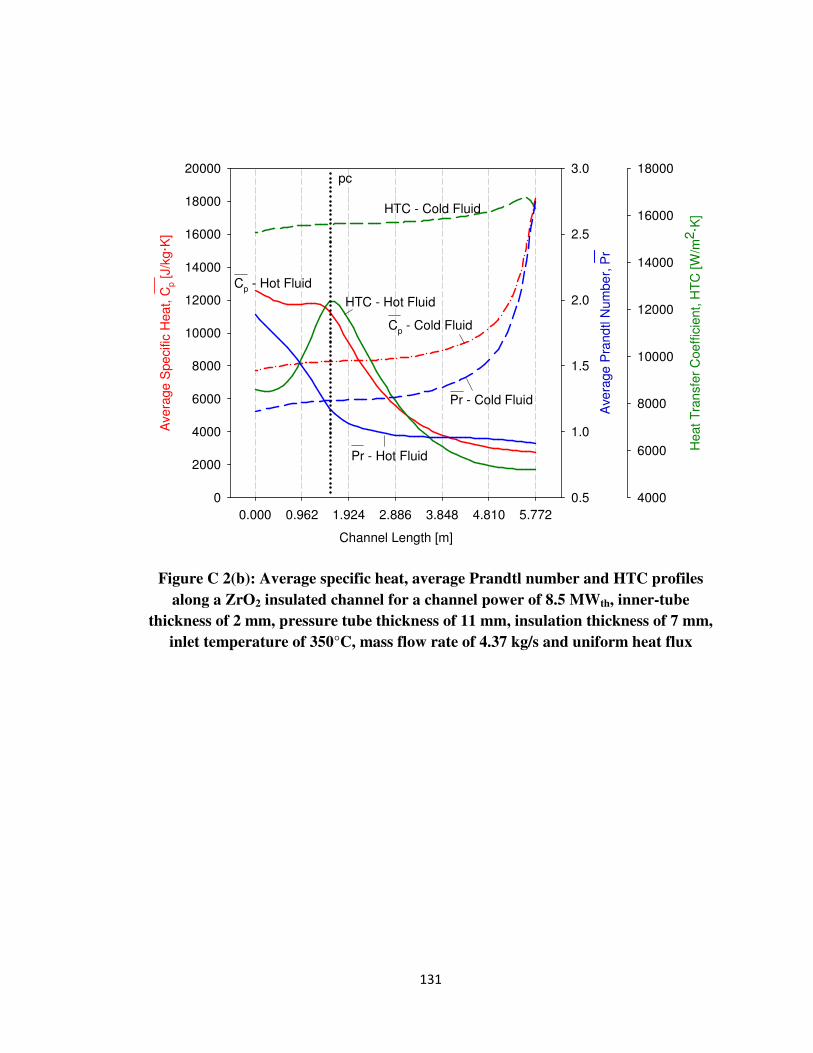
131

Channel Length [m]

0.000 0.962 1.924 2.886 3.848 4.810 5.772

Ave

rage

Specific

Heat, C

p [J/k

g·K

]

0

2000

4000

6000

8000

10000

12000

14000

16000

18000

20000

Heat T

ran

sfe

r C

oe

ffic

ient, H

TC

[W

/m2·K

]

4000

6000

8000

10000

12000

14000

16000

18000

Ave

rage

Pra

nd

tl N

um

be

r, P

r

0.5

1.0

1.5

2.0

2.5

3.0

HTC - Cold Fluid

HTC - Hot Fluid

Cp - Cold Fluid

Cp - Hot Fluid

Pr - Cold Fluid

Pr - Hot Fluid

pc





132

APPENDIX D: IMPACT OF NON-UNIFORM FLUX SHAPES –

THERMOPHYSICAL PROPERTIES

Case 2: Typical Nominal Axial Power Profile

Channel Length [m]

0.000 0.962 1.924 2.886 3.848 4.810 5.772

Th

erm

al C

on

du

ctivity,

k [W

/mK

]

0.0

0.1

0.2

0.3

0.4

0.5

0.6

Pra

nd

tl N

um

be

r, P

r0

2

4

6

8

10

Sp

ecific

He

at, C

p [J/k

g·K

]

0

20000

40000

60000

80000

k - Cold Fluid

k - Hot Fluid

Pr - Cold Fluid

Pr - Hot Fluid

Cp - Cold Fluid

Cp - Hot Fluid

pc


profiles along a 7 mm thick Porous YSZ insulated channel for a total channel power



133

Channel Length [m]

0.000 0.962 1.924 2.886 3.848 4.810 5.772

Ave

rag

e S

pe

cific

He

at, C

p [J/k

g·K

]

0

5000

10000

15000

20000

25000

30000

He

at T

ran

sfe

r C

oeffic

ient, H

TC

[W

/m2

·K]

4000

6000

8000

10000

12000

14000

16000

18000

20000

22000

24000

Ave

rag

e P

ran

dtl N

um

be

r, P

r

0.5

1.0

1.5

2.0

2.5

3.0

3.5

4.0

HTC - Cold Fluid

HTC - Hot Fluid

Cp - Cold Fluid

Cp - Hot Fluid

Pr - Cold Fluid

Pr - Hot Fluid

pc

Figure D.2 (b): Case 2 - Average specific heat, average Prandtl number and HTC


of 8.5 MW, inner-tube thickness of 2 mm, pressure tube thickness of 11 mm, inlet


134

Case 3: Peaked Shape Axial Power Profile

Channel Length [m]

0.000 0.962 1.924 2.886 3.848 4.810 5.772

Th

erm

al C

on

du

ctivity,

k [W

/mK

]

0.0

0.1

0.2

0.3

0.4

0.5

0.6

Pra

nd

tl N

um

be

r, P

r

0

2

4

6

8

10

Sp

ecific

He

at, C

p [J/k

g·K

]

0

20000

40000

60000

80000

k - Cold Fluid

k - Hot Fluid

Pr - Cold Fluid

Pr - Hot Fluid

Cp - Cold Fluid

Cp - Hot Fluid

pc





135

Channel Length [m]

0.000 0.962 1.924 2.886 3.848 4.810 5.772

Ave

rag

e S

pe

cific

He

at, C

p [J/k

g·K

]

0

5000

10000

15000

20000

25000

30000

He

at T

ran

sfe

r C

oeffic

ient, H

TC

[W

/m2

·K]

0

5000

10000

15000

20000

25000

Ave

rag

e P

ran

dtl N

um

be

r, P

r

0

1

2

3

4

5

HTC - Cold Fluid

HTC - Hot Fluid

Cp - Cold Fluid

Cp - Hot Fluid

Pr - Cold Fluid

Pr - Hot Fluid

pc





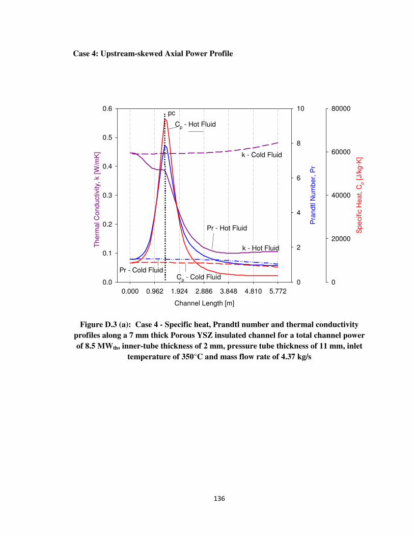
136

Case 4: Upstream-skewed Axial Power Profile

Channel Length [m]

0.000 0.962 1.924 2.886 3.848 4.810 5.772

Th

erm

al C

on

du

ctivity,

k [W

/mK

]

0.0

0.1

0.2

0.3

0.4

0.5

0.6

Pra

nd

tl N

um

be

r, P

r

0

2

4

6

8

10

Sp

ecific

He

at, C

p [J/k

g·K

]

0

20000

40000

60000

80000

k - Cold Fluid

k - Hot Fluid

Pr - Cold Fluid

Pr - Hot Fluid

Cp - Cold Fluid

Cp - Hot Fluid

pc





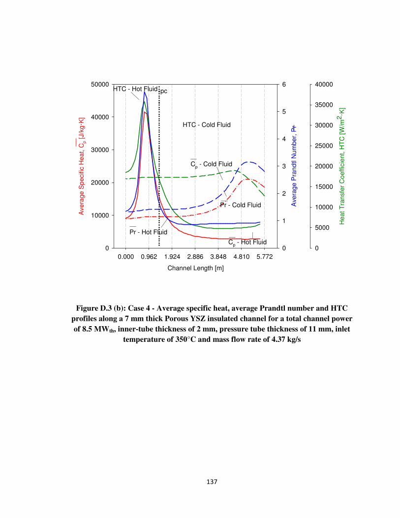
137

Channel Length [m]

0.000 0.962 1.924 2.886 3.848 4.810 5.772

Ave

rag

e S

pe

cific

He

at, C

p [J/k

g·K

]

0

10000

20000

30000

40000

50000

He

at T

ran

sfe

r C

oeffic

ient, H

TC

[W

/m2

·K]

0

5000

10000

15000

20000

25000

30000

35000

40000

Ave

rag

e P

ran

dtl N

um

be

r, P

r

0

1

2

3

4

5

6

HTC - Cold Fluid

HTC - Hot Fluid

Cp - Cold Fluid

Cp - Hot Fluid

Pr - Cold Fluid

Pr - Hot Fluid

pc





138

Case 5: Downstream-skewed Axial Power Profile

Channel Length [m]

0.000 0.962 1.924 2.886 3.848 4.810 5.772

Th

erm

al C

on

du

ctivity,

k [W

/mK

]

0.0

0.1

0.2

0.3

0.4

0.5

0.6

Pra

nd

tl N

um

be

r, P

r

0

2

4

6

8

10

Sp

ecific

He

at, C

p [J/k

g·K

]

0

20000

40000

60000

80000

k - Cold Fluid

k - Hot FluidPr - Cold Fluid

Pr - Hot Fluid

Cp - Cold Fluid

Cp - Hot Fluid

pc





139

Channel Length [m]

0.000 0.962 1.924 2.886 3.848 4.810 5.772

Ave

rag

e S

pe

cific

He

at, C

p [J/k

g·K

]

2000

4000

6000

8000

10000

12000

14000

16000

18000

20000

22000

He

at T

ran

sfe

r C

oeffic

ient, H

TC

[W

/m2

·K]

2000

4000

6000

8000

10000

12000

14000

16000

18000

20000

22000

Ave

rag

e P

ran

dtl N

um

be

r, P

r

0.5

1.0

1.5

2.0

2.5

3.0

3.5

HTC - Cold Fluid

HTC - Hot Fluid

Cp - Cold Fluid

Cp - Hot Fluid

Pr - Cold Fluid

Pr - Hot Fluid

pc





140

Case 6: Variable Axial Power Profile

Channel Length [m]

0.000 0.962 1.924 2.886 3.848 4.810 5.772

Th

erm

al C

on

du

ctivity,

k [W

/mK

]

0.0

0.1

0.2

0.3

0.4

0.5

0.6

Pra

nd

tl N

um

be

r, P

r

0

2

4

6

8

10

Sp

ecific

He

at, C

p [J/k

g·K

]

0

20000

40000

60000

80000

k - Cold Fluid

k - Hot Fluid

Pr - Cold Fluid

Pr - Hot Fluid

Cp - Cold Fluid

Cp - Hot Fluid

pc





141

Channel Length [m]

0.000 0.962 1.924 2.886 3.848 4.810 5.772

Ave

rag

e S

pe

cific

He

at, C

p [J/k

g·K

]

0

5000

10000

15000

20000

25000

30000

He

at T

ran

sfe

r C

oeffic

ient, H

TC

[W

/m2

·K]

4000

6000

8000

10000

12000

14000

16000

18000

20000

22000

24000

Ave

rag

e P

ran

dtl N

um

be

r, P

r

0.5

1.0

1.5

2.0

2.5

3.0

3.5

4.0

HTC - Cold Fluid

HTC - Hot Fluid

Cp - Cold Fluid

Cp - Hot Fluid

Pr - Cold Fluid

Pr - Hot Fluid

pc





142

APPENDIX E: CONTRIBUTIONS TO KNOWLEDGE

Refereed Conference Proceedings

Samuel, J., Harvel, G., & Pioro., I. “Design Concept and Heat Transfer Analysis for a

Double Pipe Channel for SCWR Type Reactors”, Proceedings of the International

Conference on Nuclear Engineering (ICONE-18), Xi’an, China, 2010, May 17-21.

Pioro, I., Mokry, S., Peiman, W., Saltanov, Eu., Thind, H., Grande, L., Samuel, J. and

Harvel, G., 2010. Supercritical Water-Cooled Nuclear Reactors: Thermodynamic-Cycles

Plant Layouts and Thermal Aspects of Pressure-Channel Design, Transactions of the

European Nuclear Conference (ENC 2010), Barcelona, Spain, May 30 − June 2.

Samuel. J., Harvel, G., and Pioro, I., “Heat Loss Analysis of a Re-Entrant Fuel Channel

for SCWR Type Reactors”, Proceedings of the 5th

International Symposium on

Supercritical Water-Cooled Reactors (ISSCWR-5), Vancouver, Canada, 2011, Mar 13-

16.

Samuel, J., Harvel, G., & Pioro., I. “Moderator Heat Loss Analysis of a Ceramic

Insulated Re-Entrant SCWR Fuel-Channel”, Proceedings of the International Conference

on Nuclear Engineering (ICONE-19), Chiba, Japan, 2011, May 15-19.

Technical Reports

Peiman, W., Richards, G., Samuel, J., Grande, L., Harvel, G. and Pioro, I., 2010. Key

Thermalhydraulic and Material Parameters for Fuel-Channel Design, Report for

NSERC/NRCan/AECL Generation IV Energy Technologies Program (NNAPJ) entitled

“Alternative Fuel-Channel Design for SCWR” with Atomic Energy of Canada Ltd.,

Version 1, UOIT, Oshawa, ON, Canada, December, 42 pages.

Pioro, I., Saltanov, Eu., Naidin, M., King, K., Farah, A., Peiman, W., Mokry, S., Grande,

L., Thind, H., Samuel, J. and Harvel, G., 2010. Steam-Reheat Option in SCWRs and

Experimental BWRs, Report for NSERC/NRCan/AECL Generation IV Energy

Technologies Program (NNAPJ) entitled “Alternative Fuel-Channel Design for SCWR”

with Atomic Energy of Canada Ltd., Version 1, UOIT, Oshawa, ON, Canada, March, 128

pages

conceptual design for a re-entrant type fuel channel for

Documents