Condition Monitoring of

Bolted Joints

Stephen Joseph Temitope

Thesis submitted for the degree of Doctor of Philosophy

Department of Mechanical Engineering

The University of Sheffield

June 2015

i

Abstract

Rail joints have been in existence for a long time of which their design has remained

primarily unchanged over this period. Rail joints are a typical example of bolted joints. Like

other bolted joints, their integrity depends on the quantitative representation of the contact

pressure distribution at the interface during design. In service, rail joints are subjected to

complex operating stresses, and they demand high maintenance cost because they are safety

critical and have the lowest service life of the components on the rail tracks. In this study,

non-intrusive ultrasonic techniques have been employed to investigate the parameter

relevant to their design, operation and condition monitoring.

The effect of variation in plate thickness and diameter of the bearing surface of the bolt

head on the contact pressure distribution at bolted interfaces under varying axial loads was

investigated. While it was observed that the contact pressure at the interface increases as

the applied load increases, the distance from the edge of the bolt hole at which the

distribution becomes stable is independent of the applied load on the bolted joint. However,

the contact pressure distribution was observed to vary with the plate thickness. Although the

variation in the peak value of average contact pressure distribution in bolted joints does not

depend on the plate thickness, the distance from the edge of bolt hole at which the value of

the distribution becomes stable increases as the plate thickness is increased. It was revealed

that the peak value of the contact pressure distribution decreases as bearing diameter of the

bolt head increases, and that the distance at which the normalised average contact pressure

distributions become fairly constant also increases as the bearing diameter of the bolt head

increases. In the majority of the cases, the distance falls between 3 and 4 of the bolt radius

from the edge of the bolt hole. It was also observed that the edge of the bolt head has a

pronounced effect on the position of the peak value of the contact pressure distribution at

the interface. Furthermore, a model based on a Weibull distribution has been proposed to fit

the experimental data, and a good correlation was observed.

Non-intrusive experimental techniques were simultaneously used to investigate the

relaxation of contact pressure and loosening of bolted joints subjected to cyclic shear loading.

Three critical areas: the contact interface of bolted component, the bolt length and the

rotation of the bolt head, were monitored during loosening of the joints. The results show

that loosening of bolted joints can be grouped into four stages. The early stage of the

loosening of bolted joints is characterised by cyclic strain ratcheting- loosening of the bolted

ii

joint during vibration without rotation of the bolt head. The higher the rate of relaxation at

this early stage the lower is the resistance of the bolted joint to vibration induced loosening

of bolted joints. Furthermore, the rate of loosening at the bolted joint interface is not the

same but increases away from the bolt hole. While the rate of loosening of bolted joints

largely depends on the amplitude and the number of cycles of the applied dynamic shear

load, it is independent of the frequency of the applied load. In addition, increasing the bolt

torque was found to increase the loosening resistance of the bolted joint. When joints are

subjected to a constant shear load in addition to the dynamic shear load, the loosening rate

increase, and this rate depend on the magnitude of this constant shear load.

A normal incidence pulse-echo ultrasonic technique was used to monitor de-bonding at

the interface of adhesive bonded insulated lap joints and insulated block joints, subjected to

a shear load induced failure. The results revealed that the insulated joint exhibited elastic

behaviour before a sudden failure (rupture) of the joint. The de-bonding of

adhesive/insulating layer on the web sides of IBJs was found to occur earlier than at any

other parts of the joint when the applied load was only a fraction of the peak of the shear

load. However, the de-bonding at the top and foot of the rail occurred almost at the peak of

the shear load. This same technique was used to monitor the degradation, and eventual

failure of IBJs subjected to cyclic shear loading. The results showed that the degradation of

the adhesive insulating layer has commenced, and was in progress when the joint was

virtually intact and displayed elastic behaviours. The failure at the adhesive interface is

indicated by a sudden change in the value of the measured reflection coefficient. After this,

the failure of the joint is preceded by plastic behaviour of the joint. In addition, the change in

the length of the bolts can also be monitored directly, as a complete failure at the interface of

the bolted joints can be highlighted before the failure occurred. The results of this study have

shown that, with further development, ultrasound can be used to monitor the condition of

IBJs while in service.

iii

Acknowledgements

I would like to acknowledge the encouragement, inspiration and guidance provided by my

supervisors throughout the duration of this project. Special thanks go to Dr Matthew

Marshall, my first supervisor. His help makes accomplishment of this thesis work possible.

His profound knowledge in ultrasonic and tribology has greatly enriched my understandings.

The knowledge gained from his attitude towards scientific research will be a lifetime benefit

to me. Thanks also to Prof. Roger Lewis for his criticism and advice that are of benefit to the

doctoral study, and for other supports provided in the doctoral training program.

I am grateful to the Tertiary Education Trust Fund (TETFUND), Nigeria for providing the

scholarship that funded my PhD. I also wish to acknowledge the magnanimity of Ekiti State

Universities for giving me the opportunity to do my PhD in one of the world renowned

universities. My thanks go to the staff of the Department of Mechanical Engineering, Ekiti

State University for the sacrifice made during my leaves for the PhD programme. Thanks to

Prof. S. B. Adeyemo and Dr I. O. Oluwaleye for their encouragement and advice during this

period.

My thanks go to my family for their immeasurable love, understanding, encouragement

and patience, and particularly my wife Shelter Oluwakemi, during this period of being away

from them. The sacrifice they made is immensely acknowledged. To my parent and my

siblings, I say thank you for all the encouragement, support and love.

I would like to acknowledge the excellent working relationship provided by the Leonardo

Centre for Tribology Group. In particular, I would like to thank Robin Mills, Tom Howard,

David Butcher, Gbenga Adeyemi, Julius Abere and others that provide useful attentions,

discussions and suggestions towards the successful completion of this doctoral study.

I also recognize and appreciate the effort of my friend David Akindele, my Nigerian

colleagues in Sheffield: Olatunde Ojo, Benjamin Oluwadare, Mayowa Famuyiwa, Oku Nyong,

Emamode Ubogu and others who are also important but could not mention due to space

constraint. Thanks for supporting and encouraging me at the necessary periods. My thanks

also go to the people I have met in this country who added colour to the dull days.

Finally and most importantly, I thank God for his abundant grace that see me through the doctoral study.

iv

Nomenclature

a Bolt radius (m)

ci Longitudinal speed of sound in a given medium i (m/s)

dc, lw, Diameter of piezo-crystal and focal length of transducer respectively (m)

Ultrasonic wave Frequency (Hz)

K Interfacial stiffness (Pa/m)

P Contact pressure (Pa)

q Mean stress (Pa)

r Radius distance along the plate interface from centre of the hole bolt (m)

R Reflection coefficient of an ultrasonic wave incident at boundary of two materials

u Separation of the mean lines of roughness of the two surfaces (m)

Zi Acoustic impedance of a given body i (Ns/m3)

ω Ultrasonic wave angular frequency (rad/s)

Amplitude parameter

η, β, ϒ Weibull parameters

θi, θr Angle of incidence and refraction respectively (degrees)

v

Table of Contents

Abstract

Acknowledgements

Table of Contents

Nomenclature

Chapter 1 Introduction ................................................................................................... 1

1.1 Statement of the Problem ........................................................................................... 1

1.2 Research Objectives .................................................................................................... 4

1.3 Layout of Thesis ........................................................................................................... 4

Chapter 2 Literature Review ........................................................................................... 6

2.1 Introduction ................................................................................................................. 6

2.2 Bolted Joints ................................................................................................................ 7

2.3 Failure of Bolted Joints ................................................................................................ 8

2.4 Prevention of Loosening in Bolted Joints .................................................................... 9

2.5 Investigations of Contact Pressure Distribution in Bolted Joints .............................. 10

2.5.1 Analytical and numerical studies of contact pressure distribution in bolted

joints .................................................................................................................. 10

2.5.2 Experimental studies of contact pressure distribution in bolted joints ............ 12

2.5.3 Models to fit experimental data of pressure distribution in bolted joints ........ 14

2.6 Loosening of Bolted Joints under Dynamic Loading .................................................. 15

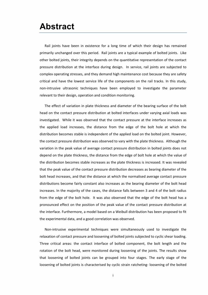
2.6.1 Self-loosening of bolted joints due to dynamic axial loading ............................ 16

2.6.2 Self-loosening of bolted joints due to dynamic transverse loading .................. 17

2.6.3 Self-loosening of bolted joints due to slip at the interface ............................... 19

2.6.4 Stages of self-loosening of bolted joints ............................................................ 22

2.6.5 Critical relative displacement ............................................................................ 23

2.6.6 Loosening of bolted joints from bending moment ............................................ 24

2.6.7 Loosening of bolted joints by impact ................................................................. 26

2.6.8 Influence of surface coating on loosening of bolted joints ............................... 27

2.6.9 Ultrasonic studies of loosening of bolted joints ................................................ 27

2.6.10 Investigation of locking devices of bolted joints ............................................... 27

2.6.11 Condition monitoring of bolted joints ............................................................... 31

2.7 Adhesive Joints .......................................................................................................... 32

vi

2.7.1 Ultrasonic techniques ........................................................................................ 34

2.7.2 Reflected normal and oblique incidence waves in time domain ....................... 35

2.7.3 Reflected ultrasonic incidence waves in frequency domain ............................. 37

2.7.4 Ultrasonic spectroscopy ..................................................................................... 38

2.7.5 Guided waves ..................................................................................................... 39

2.7.6 Bond testers ....................................................................................................... 39

2.8 Rail Joints ................................................................................................................... 41

2.8.1 Joint design and materials ................................................................................. 41

2.8.2 Supporting structure and wheel-track interaction ............................................ 42

2.8.3 Condition monitoring of IBJs ............................................................................. 46

2.9 Conclusions ................................................................................................................ 47

Chapter 3 Experimental Techniques .............................................................................. 48

3.1 Ultrasonic Background .............................................................................................. 48

3.2 Mode of Transmission of Ultrasonic Waves .............................................................. 49

3.3 Ultrasound and Material Properties .......................................................................... 51

3.3.1 Speed of sound .................................................................................................. 51

3.3.2 Acoustic impedance of materials ....................................................................... 51

3.3.3 Attenuation ........................................................................................................ 52

3.4 Production of Ultrasound Waves .............................................................................. 53

3.4.1 Piezoelectric effect ............................................................................................ 54

3.4.2 Piezoelectric ultrasonic transducers .................................................................. 54

3.5 Ultrasonic Pulse ......................................................................................................... 57

3.6 Ultrasonic Couplant ................................................................................................... 58

3.7 Focusing of Transducer .............................................................................................. 59

3.8 Focused Spot Diameter ............................................................................................. 60

3.9 Ultrasonic Reflection at Rough Surface Contacts and the Spring Model .................. 61

3.10 Interfacial Stiffness and Contact Pressure Measurement ......................................... 63

3.11 Ultrasonic Apparatus ................................................................................................. 64

3.12 Scanning Apparatus ................................................................................................... 65

3.13 Scanning and Data Processing of a Non-Conformal Contact .................................... 66

3.14 Calibration Experiment for Contact Pressure ............................................................ 69

3.15 Monitoring of the Relaxation of Contact Interface under Dynamic Load ................. 70

3.16 Conclusions ................................................................................................................ 71

vii

Chapter 4 Ultrasonic Scanning of a Static Bolted Joint ................................................... 73

4.1 Introduction ............................................................................................................... 73

4.2 Experimental Procedures .......................................................................................... 75

4.2.1 Scanning tank equipment .................................................................................. 76

4.3 Static Scanning of Bolted Joints with Varying Plate Thickness .................................. 76

4.3.1 Test specimens................................................................................................... 76

4.3.2 Scanning procedure ........................................................................................... 77

4.4 Calibration ................................................................................................................. 80

4.5 Results of Static Scanning of Bolted Joints with Varying Plate Thickness ................. 81

4.6 Analysis of Bolted Joint with Varying Plate Thickness ............................................... 85

4.6.1 Average pressure line of bolted Joint of varying torque and plate thickness ... 85

4.7 Discussions on Static Scanning of Bolted Joints with Varying Plate Thickness ......... 86

4.7.1 Joint loads .......................................................................................................... 86

4.7.2 Mean normalised average contact pressure distribution ................................. 88

4.8 Static Scanning of Bolted Joints with Varying Bolt Head Diameter ........................... 90

4.8.1 Test specimens................................................................................................... 91

4.8.2 Scanning procedure ........................................................................................... 92

4.9 Result of Static Scanning of Bolted Joints with Varying Bolt Head Diameter ........... 92

4.10 Analysis of Bolted Joint with Varying Bolt Head ........................................................ 95

4.10.1 Average pressure line of bolted joint of varying torque and bolt head

diameter........................................................................................................ 95

4.11 Discussions on Static Scanning of Bolted Joints with Varying Bolt Head Diameter .. 98

4.11.1 Joint loads .......................................................................................................... 98

4.11.2 Mean normalised average contact pressure distribution ............................... 100

4.12 Conclusions .............................................................................................................. 103

Chapter 5 Weibull Modelling of Contact Pressure Distribution of Bolted Joints ............ 105

5.1 Introduction ............................................................................................................. 105

5.2 Weibull Distribution Model ..................................................................................... 106

5.3 Weibull Fitting of Contact Pressure Distribution of Bolted Joint with Varying Plate

Thickness ................................................................................................................. 108

5.4 Joint Loads for the Weibull Fit of Bolted Joint with Varying Plate Thickness .......... 112

5.5 Weibull Fitting of Contact Pressure Distribution of Bolted Joint with Varying Bolt

Head Diameter ........................................................................................................ 114

5.6 Joint Loads for the Weibull Fit of Bolted Joint with Varying Diameter of Bolt

Head......................................................................................................................... 120

viii

5.7 Discussion ................................................................................................................ 122

5.8 Conclusions .............................................................................................................. 124

Chapter 6 Relaxation of Clamping Pressure of Dynamic Bolted Joints ........................... 125

6.1 Introduction ............................................................................................................. 125

6.2 Experimental Procedure .......................................................................................... 128

6.2.1 Test specimens................................................................................................. 128

6.2.2 Instrumentation of the specimen .................................................................... 129

6.2.3 Ultrasonic Equipment for Dynamic Bolted Joint Experiments ........................ 134

6.3 Determination of Angle of Rotation ........................................................................ 137

6.3.1 Image acquisition ............................................................................................. 138

6.3.2 Image processing ............................................................................................. 139

6.4 Dynamic Loosening Test Rig .................................................................................... 142

6.5 Dynamic Loosening Test .......................................................................................... 144

6.6 Results ..................................................................................................................... 148

6.6.1 Loosening of joint with 8 transducer array ...................................................... 148

6.6.2 Loosening of joint with 32 transducer array .................................................... 153

6.6.3 Bolt torque and cyclic shear load ..................................................................... 155

6.6.4 Transverse side load and frequency ................................................................ 159

6.7 Discussion ................................................................................................................ 161

6.7.1 Features of the results profile ......................................................................... 162

6.7.2 Phases of loosening ......................................................................................... 164

6.7.3 Initiation of loosening and ratchetting ............................................................ 165

6.7.4 Differential loosening and slip ......................................................................... 166

6.7.5 Effect of bolt torque ........................................................................................ 168

6.7.6 Effects of frequency ......................................................................................... 171

6.7.7 Effect of cyclic shear load ................................................................................ 171

6.7.8 Effect of transverse side load .......................................................................... 172

6.8 Conclusions .............................................................................................................. 173

Chapter 7 Ultrasonic Study of Adhesive Insulated Joints .............................................. 176

7.1 Introduction ............................................................................................................. 176

7.1.1 Experimental procedure .................................................................................. 177

7.2 Tensile Lap Shear Test on Adhesive Bonded Insulated Joints ................................. 178

7.2.1 Tensile lap shear test specimen ....................................................................... 178

ix

7.2.2 Instrumentation of specimens ......................................................................... 180

7.2.3 Test Procedure for the tensile lap-shear test .................................................. 181

7.2.4 Results .............................................................................................................. 182

7.2.5 Discussion ........................................................................................................ 187

7.3 Shear Test of Insulated Block Joint .......................................................................... 189

7.3.1 Instrumentation of the insulated block joint specimens ................................. 190

7.3.2 Shear test of the IBJs ........................................................................................ 191

7.3.3 Results .............................................................................................................. 193

7.3.4 Discussion ........................................................................................................ 198

7.4 Conclusions .............................................................................................................. 200

Chapter 8 Application of Ultrasound for Condition Monitoring of Insulated block joints 202

8.1 Introduction ............................................................................................................. 202

8.2 Experimental Procedure .......................................................................................... 204

8.2.1 Test specimen .................................................................................................. 205

8.2.2 Instrumentation of the IBJ specimens ............................................................. 205

8.3 Dynamic Shear Test of the IBJs ................................................................................ 207

8.4 Results ..................................................................................................................... 209

8.5 Discussion ................................................................................................................ 216

8.6 Conclusions .............................................................................................................. 218

Chapter 9 Conclusions and Recommendations ............................................................ 219

9.1 Conclusions .............................................................................................................. 219

9.1.1 Contact pressure distribution in bolted joints ................................................. 219

9.1.2 Relaxation of contact pressure and loosening of bolted joints ....................... 221

9.1.3 Shear failure of adhesive bonded insulated joints .......................................... 222

9.1.4 Condition monitoring of insulated block joints under dynamic load .............. 223

9.2 Recommendations for Future Work ........................................................................ 223

Publication Arising from this Work…………………………….……………………..…………………………….…225

References…………………………..……….…………………………………………………..….………………………….…226

1

Chapter 1 Introduction

Introduction

1. A rail joint is a feature of railway track that has existed for almost two centuries,

during which its design has changed little. A rail joint possesses lower vertical

bending stiffness when compared to the connecting rails, and has the lowest

service life of the components on the rail tracks. As a result of this weakness and

coupled with the increasing axle loads and tonnage speed on the rail tracks, the

rail section in the vicinity of the rail joints also suffered a short service life.

Recently, they have been replaced by continuous welded rail, but still retained as

a necessary component in some parts of the tracks for engineering and economic

reasons. They are safety critical components on the rail track and demand a high

maintenance cost. In the present research work, studies will be conducted on a

relevant parameter of their design and the technique for their condition

monitoring in service. The statement of the problem, the objectives of the

research and the thesis layout will be discussed in this chapter.

1.1 Statement of the Problem

Railways emerged in Europe in the second quarter of the 19th century as a new transport

mode and thereafter became the main inland transport mode for carrying passengers and

freight which brought about big changes in transport, economy and society [1, 2]. In the

quest to make rail transport more efficient, railroads administrators have consistently been

searching for methods of carrying more weight on trains at higher speeds. This in turn has

placed high stresses on the trains, the rail and rail components over which these high

tonnage trains travel. One of the important rail components that are affected by these

elevated stresses are the rail joints.

Rails are manufactured in relatively short lengths of 60 metres to 120 metres of different

sizes, and they are required to be attached to one another, end to end, during installation.

Rail joints are points at which these short length segments of rails are structurally connected.

They are joined by either welding or mechanical connections. The mechanical connectors

consist primarily of fishplates and mechanical fasteners (bolts and nuts) that mount the

fishplates to the web sides of the rail. Hence, a mechanical rail joint is a typical example of

2

bolted joints. Rail joints can be categorised as conductive rail joints and insulated block joints

(IBJs) depending on their operation. While the conductive joints allow electricity to pass

through it to the adjoining rails, the insulated block joint electrically isolates the connecting

rails. Figure 1.1 shows examples of the rail joints.

Figure 1.1: Rail joints; (a) A-4 bolt conductive rail joint [3]and (b) Glue Insulated

Block Joint [4].

Rail joints are weak spots on the rail track with a short service life; they have the least

service life compared to other running surface components in rail tracks. Their service life in

arduous conditions is typically a third of a rail life subjected to high traffic and track load [5].

Apart from their short service life, they introduce large deflections in the track under the

passing wheel which result in large dynamic loads that cause track deterioration around their

vicinity.

As a result of the drawbacks that associated with rail joints, they have been removed from

many points in the railway mainlines and replaced by welded rail joints to produce tracks of

continuous welded rail (CWR). Presently, the mechanical joints are used in railway to connect

strings of continuously welded rail together for engineering and economic reasons. However,

they are still prominent in sharp curves and other places where there is a need for quick

replacement of worn rails. The IBJs are essential in the traffic controlling system on the

railway tracks where they are used to form rail into isolated blocks or segments that are

electrically isolated from each other. This is for the purpose of allowing railway signalling

system to locate train by maintaining a shorting circuit system. This also enables the

detection of broken rails in the track.

The failures of rail joints can be classified into mechanical/structural, and electrical failures

in the case of IBJs. The mechanical/structural failures includes weakening of the adhesive

bonds which lend strength to the joints, loosening of bolts, cracked or missing bolts, cracked

joint bars, bolt hole cracks in rail, battered rail ends and excessive shelling on the rail head

3

[5]. The electrical failures are caused by metal surfaces coming into contact. Sometimes

electrical failures are one of the end products of mechanical degradation of a joint that allows

increased deflection and prevents distribution of loads effectively across the substructure

which subsequently results in localized damage to the track structure (plastic deformation of

rail end). The mechanical/structural failures of insulated joints are initiated and propagated

by the adhesive bond failure at the interfaces and loosening of joint’s bolts, and in most cases

are hard to detect at the onset. A timely intervention will prevent deterioration of the joints

to a stage that it failure will affect other components of the track.

The failure of rail joints causes substantial disruption to railroad operation and in some

cases, they are of fatal consequence. Hence, they are safety critical components of the rail

track structure [6-8]. Due to their importance in the safety and operational efficiency of the

railroad, their maintenance places a high demand and huge cost on the rail industry. It is on

record that UK network currently has around 80,000 installed insulated block joints. Due to

failures, these joints contribute towards 1,800 delays causing incidents over a period of two

years at a cost of approximately ten million pounds [9]. Presently, visual inspection is being

employed to detect battered rail edges, loose and missing bolts, crack fishplates, evidence of

longitudinal movement and debonding of the insulator at the edge of the fishplate in

insulated block joints, and this is labour intensive. Therefore, study to improve the

performance of this rail component through design and also to monitor their performance in

service has been a targeted focus of the engineering community.

As mentioned earlier, rail joints are a typical example of bolted joints. Their integrity (i.e.

stiffness and performance), like bolted joints, depends on quantitative representation of

contact pressure distribution at the interface during design. Presently, their design and

evaluation is based on theoretical analysis, with assumptions, to quantify the pressure

distribution at the clamped interface, which may not represent their true operating

conditions. This is due to the difficulty in reaching and assessing clamped interfaces with

traditional experimental methods. In addition, it is possible in principle to design bolted

joints that will overcome the service load without unintentional loosening [10, 11]. However,

in practice bolted joints loosen in service when subjected to dynamic loads.

Therefore, it is not only important to understand the loosening mechanism in bolted joints

and existing design parameters for optimised resistance to loosening, but monitoring of such

phenomenon in service is also very important especially when their operations are safety

critical. Therefore, in this study, there are some issues that will be dealt with. The first is an

experimental investigation of contact pressure distribution and the contact size in the bolted

4

joint interface with a variable plate thickness and bolt head using a non-intrusive technique.

The second is the development of a model that fit the experimental investigation data and

represents the contact pressure distribution in the bolted joint interface. The third part will

involve the study of relaxation of contact pressure in the bolted joint and hence, the

loosening mechanism of dynamic loaded bolted joint. Lastly, investigations will be conducted

on the mode of failure propagation in insulated adhesive joints and the knowledge gained in

the previous studies will be used to monitor the failure of bolted insulated block joints using a

non-intrusive ultrasonic technique.

1.2 Research Objectives

This research is carried out with the aim to investigate bolted joint variables that are

crucial to the design and performance of rail joints through experimental procedures, and

also to develop an ultrasonic technique for condition monitoring of rail joints.

The following are the summarised specific objectives of the research work:

To investigate and characterise the contact pressure distribution at the interface of

bolted joints under static load using an ultrasonic technique.

To develop a model to fit the experimental data of the characterised contact pressure

distribution in bolted joint.

To investigate the relaxation of contact pressure and consequently, the loosening of

bolted joints under dynamic loading.

To develop the ultrasonic reflection technique to monitor the deterioration of

contact interface of insulated block joints subjected to dynamic loads induced failure.

1.3 Layout of Thesis

Chapter 1 of this thesis contains the statement of the problem, the objectives of the

research and the thesis layout. In Chapter 2, the outlines of the literature review on the

bolted joints; the contact pressure distribution and the loosening of bolted joints subjected to

vibration induced loosening. Furthermore, this chapter also contains literature review on the

adhesive joints and the non-destructive ultrasonic techniques of testing adhesive joints.

Previous studies on rail joints were also discussed in this chapter.

Chapter 3 presents the relevant theory behind the ultrasonic techniques. The ultrasonic

reflection from the rough surface contact and spring model approach to determine the

5

interfacial stiffness, which discloses the nature of an interface, was also discussed. A

calibration experiment that relates interfacial stiffness and contact pressure in an interface

was explained. In addition, the chapter also presents experimental equipment and

experimental procedure to obtain contact pressure of an interface. In the last section of the

chapter, the response of ultrasonic reflection to the relaxation of contact pressure at the

interface was discussed.

In Chapter 4, a non-intrusive ultrasonic technique was used to investigate and quantify the

pressure distribution in bolted joints. In the first part of this chapter, the effect of variation in

plate thickness on the contact pressure distribution at bolted interfaces under varying axial

loads was studied. While in the second part of the chapter, the effect of variation in bearing

diameter of the bolt head on the contact pressure distribution at the bolted interface under

varying axial loads was examined.

Chapter 5 presents a proposed model to fit experimental data of contact pressure

distribution in bolted joints. A statistical model based on the Weibull distribution to fit the

experimental data of the bolted joints with varying plate thickness and bolted joints with

varying diameter of the bearing surface of the bolt head was discussed. In addition, the shape

and scale parameters of the Weibull distribution and parameters introduced to adjust the

amplitude of the contact pressure distribution curve in the model were presented.

The findings from the investigation of the contact pressure distribution in the previous

chapters were used in Chapter 6 to investigate the loosening of bolted joints due to dynamic

shear loading using a non-invasive ultrasonic technique. The relaxation of contact pressure at

the bolted interface, the relaxation of the tension in the bolt and rotation of the bolt heads

were studied in the chapter to understand the mechanism of loosening in bolted joints.

Chapter 7 deals with the ultrasonic study of the interfacial response of insulated adhesive

lap joints and insulated block joints with different insulating materials subjected to failure

induced shear loading. The ultrasonic reflection from the bonded interface was used to

understand the de-bonding of adhesive at the interface of the joints, and also to establish a

method of monitoring adhesive insulated joints.

In Chapter 8, the technique discussed in the previous chapter was used to study a full scale

insulated block joints. The reflected ultrasound from the contact interface in the insulated

bolted rail joints was used to monitor the relaxation in these joints when subjected to failure

induced dynamic loading. Chapter 9 discusses the general summaries of the work done in this

study and recommendations for further research study were also given.

6

Chapter 2 Literature Review

Literature Review

2. Rail joints are important components in rail track, especially the insulated rail

joint which is part of the railway signalling system that allows for electrical

separation of two pieces of running rail whilst joining the two rails together. The

operating stresses in the insulated block joint are quite complex and their

mechanical performance depends on the developed stiffness at the bolted

interface. This is primarily a function of the bolted joint performance and the

supporting adhesive strength of the epoxy glue. Therefore, this chapter will

discuss the studies carried out on the bolted joints (contact pressure distribution

at the bolted interface and loosening of bolted joints under dynamic loading),

testing and failure of adhesive joints and last, the failure of rail joints. Studies on

the condition monitoring of bolted joints and insulated block joint will also be

discussed.

2.1 Introduction

Rail joint with fishplates was first developed and introduced to join rail ends in railway

track in 1849. As shown in Figure 1.1 in Chapter 1, the mechanical connectors consist

primarily of fishplates and mechanical fasteners (bolts and nuts) that mount the fishplates on

the web sides of the rail. Rail joints are the typical example of bolted joints. Insulated rail joint

has insulating material between the bolted interfaces. Therefore, most of the research works

on bolted joints are relevant to the design and operations of the rail joints. An exploded view

of an insulated rail joint is shown in Figure 2.1.

Figure 2.1: Exploded view of an insulated rail joint [12].

7

2.2 Bolted Joints

Bolted joints are temporary fasteners that are used to connect elements/components

together to form mechanical structures. They are extensively used in modern engineering

structures and machine design due to the following advantages [13]: high load-carrying

capacity, reliability, ease of assembly and disassembly of structures/machine components

(especially for maintenance purposes), relatively low cost and efficient manufacturing

process.

Bolted joints consist of a bolt, nut and sometimes washer, which can be considered as the

parts of the clamp members. Bolted joints connect components together through applied

clamping force provided by the tension in the bolt. The bolt has a bolt head and male

threaded shank while the nut is the female inside threaded component. Screw joints exist

where the components are joined without a nut and one of the members has the female

inner thread hole. Figure 2.2 shows vertical sectional diagrams of typical bolted and screw

joints.

(a) (b)

Figure 2.2: Vertical sectional view of (a) bolted joint and (b) screw joint.

Bolted joints came into prominence in the eighteenth century during the construction of

the “iron bridge” in Telford, and have since been used in various applications including bolted

rail joints. When a bolt is used to connect components, it provides a high clamp force that is

known as pretension or bolt preload. In a preloaded bolt, an initial tensile load is created as

soon as tightening torque is applied. Even in the absence external tensile load, this moves the

bolt head against a clamped component. The bolt head and the thread generate the preload

in the bolted joint. The more the thread mating, the more the preload is generated. When a

bolted joint is tightened, a pitch difference exists on the surface between the bolt and the

thread. If the thread is not damaged by the pitch difference, the bolt is stretched and the

resulting preload is a function of this axial elongation and joint stiffness.

8

The purpose of preload is to place the bolted components in compression for improved

resistance to either static or cyclic external loads. Preload creates a force between the bolted

joint members so that the shear load can be resisted by friction forces. Variations in the

magnitude of the preload can lead to severe changes in the cyclic life of the bolted joint.

Determination of proper preload depends on the accurate predictions of member stiffness.

The geometry and magnitude of the contact pressure at the contact interface are essential in

determining the clamping performance of the bolt and associated joint stiffness. Therefore,

the integrity of bolted joints depends on quantitative representation of the contact pressure

distribution at the interface during design.

2.3 Failure of Bolted Joints

Despite the advantages associated with bolt fasteners, it has been observed that they can

fail in operation. In some cases, the failures of bolted joints are of fatal consequences, and

hence, they are safety critical. This is illustrated by the investigated reports of the Potters bar

rail crash and Grayrigg derailment of May 2002 and February 2007 respectively. The train

derailments in both cases were as a result of relaxation and loosening of bolted joints which

was not noticed until tragedy struck due to poor maintenance regimes. 7 lives were lost and

77 injured in the train derailment in Potters bar while the Grayrigg derailment claimed 1 life

and 28 people sustained various degrees of injury [6, 7].

Among many other reported rail accidents in different parts of the world was the fatal

train derailment/crash in Rometta Marea, Messina, Italy in June 2002. The report of the

accident listed failure of bolted joints as a prime culprit [8]. A preliminary investigation into

another fatal train crash that occurred in Bretigny-sur-Orge, France in July, 2013 revealed that

loose fishplate in rail joint was the cause of the accident [14]. 7 people were killed and 200

injured in the crash. Failure of bolted joints is not restricted to railway industry alone. An

analytical review by Plaut and Davis [15] of the Tacoma Narrows Bridge accident that resulted

in its total collapse on 7th November 1940 concluded that loosening of bolts on a cable band

joint caused torsional motion of the deck, and this eventually led to the bridge’s demise.

Accidents have also been reported in the aerospace industry involving failures in control

system due to self-loosening of bolts. In 1999, a Tupolev passenger jet plane was reported to

have crashed due to self-loosening and consequent detachment of nut that connected the

pull rod to the bell crank in the elevator control system [16]. The aircraft accident report of a

Sundance helicopter crash near Las Vegas, Nevada on December 7, 2011 showed that there

was a failure of a self-locking nut that turned loose and disconnected the flight control input

9

rod. The input connects the rod to the servo that served the main rotor while the helicopter

was in flight. The failure caused loss of control and the resulting crash [17]. All the people

(61 and 6 respectively) on board were killed in the case of the mentioned crashes.

In biomedical engineering, threaded fasteners are commonly used to attach and secure

implants to bone within the body. There are reported cases of loosening of these threaded

fasteners when subjected to dynamic loads. While Becker and Becker [18] and Aboyousef et

al. [19] reported loosening of up to 43% of retaining screws in implants in the first year,

Khraisat et al. [20] reported that 26% of retaining screws in implants needed re-tightening in

the first year. Loosening of bolted joints has also been an issue in machine tools. Kaminskaya

and Lipov reported that 20% of total failures of mechanical systems of machine tools could be

traced to self-loosening of threaded fasteners. The time taken to rectify failures of such

bolted joints was estimated to represent 10% of the lifetime to a failure of a given machine

[21]. A report presented by Holmes [22] indicated that in the automobile industry, 23% of all

service problems were due to loosened bolted joints. The report further shows that loosen

fasteners were found in 12% of all new cars surveyed.

2.4 Prevention of Loosening in Bolted Joints

In order to prevent loosening of bolted joint, various techniques are recommended and

employed to maintain clamping force in the joint [23-25]. Some of these techniques are the

parameters used by joint designers during the design process and these include:

Material selection by the designer to enhance friction between the clamped

surfaces. Matching of materials at the joint to guarantee sufficient clamping force at

varying service temperatures.

Design of mating material components with minimal clearance.

Design of joint for high preload application (this improves friction between the

contacting surfaces of the bolted joint thereby increasing vibration induced

loosening resistance).

Design of joint with a high ratio of bolt length to diameter (this is also good, to

compensate for any misalignment between clamped component).

Reorientation of the joint so that it can be subjected to loading in an axial direction,

instead of shear loading.

In theory, it is possible to design a joint that will retain a sufficient prevailing (residual)

torque to overcome the service load without rotational loosening even in the absence of any

10

locking device [10, 11, 26]. However, in practice, bolted joints do turn loose. Furthermore, a

detailed procedure for the design of bolted joint of this nature requires full information of all

forces on the joint and, most times, such knowledge is not available. Hence, designers

commonly specify the use of a fastener locking device on the fastener in a joint during

installation to prevent loosening. Fastener locking methods such as an adhesive thread-

locking liquid chemicals such as ‘Loctite’ and ‘Precote’, prevailing torque locking nuts, cotter

pin and castle nut, multiple bolts locked together using safety-wires, restraining plates,

ratcheted washers, modified threaded fasteners (bolt and nut) and use of two nuts are

usually employed. The success of these locking methods depends on the amount of the bolt

pre-load that can be maintained for a given vibration cycle. The majority of the locking

devices do not totally lock the fastener, but tolerate some degree of self-loosening under

dynamic shear loading [27, 28].

2.5 Investigations of Contact Pressure Distribution in Bolted

Joints

Bolted joints have been a focus of many investigations, many of these studies involved

analytical and numerical models to predict the contact pressure distribution in the interface

of bolted joints. Some other researchers have used experimental approaches in their

investigations to know the geometry and the magnitude of the contact pressure in the

clamped interface of bolted joints. Some of the studies carried out using these methods are

discussed in the following sections.

2.5.1 Analytical and numerical studies of contact pressure

distribution in bolted joints

Analytical models have been developed to predict the pressure distribution in bolted

joints as a function of the contact radius. The results from the models also depended on the

plate thickness and the bolt head radius. According to Fernlund [29], Rotscher was one of the

early researchers to calculate the spread of stress in a bolted joint. He believed that for joint

of the same material, the joint stress spread within a frustum cone of semi-angle of 450, and

that the interfacial pressure is constant within the contact radius. Although, the hypothesis

was considered not to describe the pressure distribution satisfactorily, it was the first

approximation for the contact zone and is expressed as:

𝑐 = 𝑏 + 𝑡(𝑡𝑎𝑛𝛼) 2.1

11

where c is the radius of the contact zone, b and t is the bolt head radius and plate

thickness respectively.

Shigley and Mischike [13] and Lehnhoff et al. [30] believed that the pressure angle of 450

proposed by Rotscher overestimates the clamping zone. They proposed an analytical model

to calculate the member stiffness and the stress distribution of bolted joints for various bolt

sizes, thicknesses and materials of the members. It was assumed that there was a uniform

pressure within a frustum cone envelope under the bolt head. They recommended a fixed

standard pressure angle of 300 as a better value for calculating the joint material stiffness:

𝐾𝑚 =𝜋𝐸𝑑𝑡𝑎𝑛𝛼

2𝐼𝑛[(𝑙𝑡𝑎𝑛𝛼+𝑑𝑤−𝑑)(𝑑𝑤+𝑑)

(𝑙𝑡𝑎𝑛𝛼+𝑑𝑤+𝑑)(𝛾𝑑−𝑑)⁄ ] 2.2

where Km is the joint member stiffness, E is the Young’s modulus of the clamped material,

d the bolt diameter, dw the diameter of the contact under the bolt head, l the effective grip

and the contact radii ratio.

Fernlund [29, 31], Greenwood [32], Lardner [33], Motosh [34] and Chandrashekhara and

Muthanna [35] used analytical methods (Hankel transformation method and Fourier-Bessel

series) from the theory of elasticity to obtain the pressure distribution on the interface of two

bolted plates as a function of bolt radius, by considering the two plates as a single plate of

identical material and thickness which is equal to the combined thicknesses. The interfacial

contact pressure between the two plates was also assumed to be equal to the stress at the

mean plane of the single plate. The pressure was represented by a polynomial of fourth

order, which is a function of the non-dimensional radius r/a. They claimed that the contact

pressure tends to zero at a distance equal to or greater than five times the non-dimensional

radius r/a, and that Poisson’s ratio is the only material property that affects pressure

distribution in bolted joints.

However, Chandrashekhara and Muthanna [36] noted that single plate model could only

be used to obtain the pressure distribution at the interface, only if the two bolted plates were

made of the same thickness and material. If either the thickness or the material of the plates

are not the same, then each plate must be treated as an annually loaded plate supported by

rigid bed, and the solution could be obtained by using continuity at the joint. Similarly,

numerical studies conducted by Gould and Mikic [37] to investigate the pressure distribution

in both single plate and two plate models showed that the assumption that bolted joint could

be represented by a single plate does not give the correct contact zone in a bolted interface.

In their studies, a steel of various thicknesses was modelled; the bolts were replaced by

12

uniform distributed axisymmetric loads on the connected parts of the bolted joint. They also

found out that there was a radius at which the connected flat and smooth plates become

separated, and that this radius of the contact is lower in two plate models.

Furthermore, the effect of the plate thickness ratio on the load and pressure distribution

in bolted joints was investigated by Ziada and Abed El Latif [38, 39] using FEM analysis. Unlike

previous models that used oversimplicity loading conditions in their modelling, these studies

used a more realistic external load situation by including the bolt head in its model. They

found out that the peak of the contact stress at the interface of bolted joints did not occur at

the edge of the hole; but at a point away from the bolt hole. This was due to the effect of the

geometry of the bolt head on the stress distribution. Therefore, their results showed that the

load and the pressure distribution under the bolt head are neither constant nor uniform.

However, constant amount of load and pressure occurred across the joint under the bolt

head, whatever the ratio of the two bolted plates. The peak stress was also shown to change

with an increase in top and bottom plates thickness ratio and reach its lowest when the ratio

is equal to 1. The spread of load across the joints and the separation radii of the plate at the

interface were also shown to change with an increase in thickness ratio. The separation radii

reached a maximum value of 3.5 when the ratio is 1 and decreased to an approximate value

of 2.5 as the thickness ratio is equal or greater than 10. The thickness of the thinnest plate

has a pronounced effect on the separation radius.

In addition, it was shown that the spread of loading across a joint increases with the

increase in thickness ratio and reaches its maximum at a thickness ratio of 1. As a result of

this, they expressed doubts about the presumed assumption that force is transmitted from

the bolt head to the joint part along the cones of influence. Ziada and Abed El Latif also

established that there exists a circular contact area on the interface under each bolt; which

size is independent of tightening loads on the bolt.

2.5.2 Experimental studies of contact pressure distribution in

bolted joints

Aside from modelling, experimental investigations were carried out by a good number of

authors to study the interfacial pressure distribution in bolted joints. In some of these

studies, materials were introduced in the clamped surfaces [37, 40]. Although, the results

from these studies revealed geometries of high contact zone around the bolted hole, but the

introduction of materials between the contacting surfaces would have altered the exact

13

contact pressure distribution at the interface [40]. Gould and Mikic [37] studied the

geometrical distribution of contact stress at the interface of bolted joints by coating one of

the contacting surfaces with radioactive material. The sensitive surface was later exposed to

radiographic film and developed after load had been applied to the joint. The resulted

pressure distribution and size of the contact zone are in agreement with the computational

numerical results.

Sawa et al. [40] used three methods to investigate contact pressure in bolted joint. They

used pressure sensitive films, pressure sensitive pins and ultrasonic techniques. A metallic

gasket was introduced between the clamped surfaces of the bolted joints in the case of the

experiments using pressure sensitive films and ultrasonic techniques. The results of the

experimental methods were compared with that of analytical and numerical models. They

found out that there is a point where the contacting interfaces become separated, and that

introduction of materials between the contacting surfaces will alter the exact contact

pressure distribution at the interface.

Ultrasonic techniques have been used by different authors [40-44] to investigate features

of bolted joints as viable methods to overcome the problem of the introduction of materials

between clamped surfaces. In 1979, Ito et al. [42] used an ultrasonic technique to investigate

interfacial pressure distribution on bolted flanges. They showed that the surface roughness,

material and thicknesses of the plates influenced contact radius and the pressure

distribution. Bolted Plates made of stainless steel, brass and aluminium were used with

varying applied axial forces between 9.8 kN to 19.6 kN. They concluded that the smaller the

plate thickness, the higher the contact pressure for a given axial force.

More recently among the researches in the ultrasonic area was the research works by Pau

and Baldi [41], and Baldi et al. [43] that investigated the pressure distribution in bolted joints

using plates of different thicknesses. The results of the pressure map and contact pressure

distributions were compared with results from pressure sensitive films and finite element

methods. Although plates of different thicknesses were tested, the relationship between

plate thickness and interface pressure distribution was not discussed, due to the focus of the

work being the aforementioned comparison of different investigative techniques.

Marshall et al. [44] applied an ultrasonic technique in their investigation to study bolted

surfaces with no washer, and with plain and spring washers for a series of different bolt

torques using two different interfaces. They found out that surface profile and washers affect

the spread of the contact pressure at the bolted interface. Consequently, they showed that it

14

is inappropriate to use a fixed contact spread angle, as suggested by some other studies, to

determine joint stiffness for bolted joints with different contact surface profiles.

Moreover, just like the results of the numerical models in the studies by Ziada and Abed El

Latif that used a more accurate external load situation, Marshall et al. showed that the peak

contact pressure occurred at points away from the bolt hole (as shown in Figure 2.3). This

was attributed to the effect of the edge of the bolt head on the pressure distribution. The

reasons why this effect could not be captured in some of the other studies can be ascribed to

the oversimplicity of load conditions in their models, introduction of materials into the

contact surfaces of the bolted joints and insufficient resolutions of experimental techniques.

Figure 2.3: Comparison of the published studies of bolted joint pressure distributions [44].

2.5.3 Models to fit experimental data of pressure distribution in

bolted joints

Some studies have suggested appropriate models to fit experimental data. In 1994,

Mittelbach et al. [45] conducted an experimental investigation on both the interfacial

pressure distribution and the thermal conductance in bolted joints formed by 6061-T6

aluminium plates. Pressure sensitive films were placed between loaded contacting surfaces

with the axial load varied from 6.69 kN to 13.425 kN. The experimental results were

compared with published theoretical pressure distribution models (Figure 2.4 (a)). It was

noted that while Chandrashekhara model presents higher peak pressure, the contact radius

given by Ferlund model is larger than Chandrashekhara model. They concluded that the

models presented by Fernlund and Chandrashekhara were the best to fit the experimental

results.

15

Figure 2.4: (a) Comparison of the experimental dimensionless pressure distributions as a

function of dimensionless radius for plate thickness ratios of t1/t2 =2/3, 1, and

4/3, with analyses of Chandrashekhara and Muthanna [35] and Fernlund [29],

(b) Adjustment of Weibull curves for Al-Al contact surfaces [46].

However, Mantelli et al. [46] in their published studies in 2010 highlighted the Weibull

distribution as an appropriate distribution to fit to experimental data obtained by placing

pressure sensitive film between homogenous and non-homogenous bolted interfaces. Steel-

steel and aluminium- aluminium bolted interfaces were used for the homogenous while

steel-aluminium was used for the non-homogenous bolted interface. But, as detailed in the

published paper, it was not possible to explore the relationship between Weibull and bolted

joint parameters in this study. Although the values of the Weibull parameters obtained could

not be given, a good correlation was achieved between the fits of the experimentally

measured data and the predicted contact pressure. As can be seen in Figure 2.4, the studies

showed that the Weibull distribution fits the experimental data better than models from

Fernlund and Madhusudana et al.

2.6 Loosening of Bolted Joints under Dynamic Loading

The problem of unintentional loosening of bolted joints has been identified since it came

into prominence during the industrial revolution in the nineteenth century, especially in the

rail industry. Subsequently, efforts were made to improve their design to prevent loosening

inadvertently. In the documented patent work of Alfred Buckingham Ibbotson, of Florence,

Italy, and Frederick John Talbot, of Sheffield, England in 1877 [47], it was claimed that their

improved bolt and nut design was to prevent loosening of screw nuts and screw bolt in

16

railway joints which are exposed to vibration or incursion that caused the bolts or nuts to

slack or loose, and thereby cause the unfastening or detachment of them. Henry Lawrence

and Charles H. White [48] in their invention combine a nut and bolt with a binding-screw, so

that neither bolt nor nut that secure fishplate to each side of rail joints can work loose as a

result of vibrations and incursions from passing trains.

2.6.1 Self-loosening of bolted joints due to dynamic axial loading

Although self-loosening of bolted joints had been noted since the nineteenth century,

efforts were only concentrated on the design of bolted joint fasteners to resist loosening.

There is no clear documentation on the investigation of the process that led to a loosening of

joints until 1945. The earliest research works were focused on bolted joints loosening caused

by vibration loading in the axial direction of the fasteners. Goodier and Sweeney in 1945 [49]

conducted a documented investigation on the loosening of bolted joints subjected to axial

loading and vibration (i.e. loading and vibration in the direction along to the axis of the bolts).

Loosening of bolted joints was attributed to radial contraction of the bolt due to tensile loads

and simultaneous radial dilation of the nut wall when dynamically loaded in the axial

direction with respect to the bolt (as illustrated in the exaggerated sketch in Figure 2.5). It

was believed that a further pull of the bolt in the direction of the bolt thread causes the bolt

to turn loose, and they referred to this as that of a “frictional ratchet”. Some of the bolt

parameters identified to influence loosening are thread bolt diameter, pitch, thread tolerance

and length of the bolt.

Figure 2.5: Bolt tension and nut dilation.

In 1950, Sauer et al. [50] carried out experimental work to examine the work Goodier and

Sweeney. Bolts were first subjected to a static load of 500 Ibf and various dynamic loads of

17

400 Lbf and 450lbf were then superimposed on the static load in a fatigue testing machine.

Although, the amount of loosening recorded in this study is very small (less than 6 degrees of

bolt rotation) but is greater than what was observed by Goodier and Sweeney. From the

results, it was discovered that the rate of loosening in bolted joints under dynamic axial

loading is usually large at first, and this diminishes rapidly as the number of cycle increases. It

was also found out that clean and smooth surface of joint components improved the contact

frictional force between components, thus reduced the rate of loosening. An increase in

preload was also found to decrease the amount of loosening. While the rate of loosening

increase with an increase in the ratio of dynamic load to static load, they revealed that the

rate of loosening decrease significantly with previously used nuts when compared to new

(unused) nuts.

2.6.2 Self-loosening of bolted joints due to dynamic transverse

loading

The key theory of vibrating loosening under dynamic transverse loads (i.e. loading and

vibration in the direction perpendicular to the centre of the bolts) was explained by Gerhard

H. Junker in his influential paper on the self-loosening of threaded fastener in 1960 [51]. He

indicated that apart from fatigue failure, self-loosening induced by vibration is the major

cause of failure in bolted joint subjected to dynamic loads. It was explained that once an

external force in one direction overcomes the force of friction between two solid bodies,

force smaller than the friction force can cause movement to occur in any other directions.

Therefore, loosening results from relative movement between the threads of the bolt and nut

after the frictional force between these two surfaces has been overcome.

As explained by Junker, the concept of loosening could be illustrated by considering the

threads of the bolt as an inclined plane. While the nut is viewed as a block on the inclined

plane as shown in Figure 2.6 (a). The block will remain at rest (equilibrium) on the inclined

plane as long as there is no external force acting on it and the existing force of friction

between the two bodies is greater than zero.

18

(a) (b)

Figure 2.6: (a) Block on incline plane and (b) Bolted joint subjected to dynamic shear load.

If the inclined plane is subjected to transverse vibration, the block will not only move in

the transverse direction. It will slip down the plane if its inertial force is greater than the force

of frictions between the surfaces. Applying this to Figure 2.6(b), which consists of a clamped

component attached to a fixed base with a preloaded bolt. Junker stated that when applied

shear forces exceed the frictional force in the transverse direction, the joint will be free of

friction force in any other direction. Hence, the turning moment due to a helix form of the

bolt thread and stored torsion developed during tightening of bolt provides a loosening

moment at the commencement of a loosening. As indicated in the study, this mechanism can

completely loosen fasteners under a repetitive transverse movement. He concluded that

transverse vibration was most severe loading condition to induce self-loosening in bolted

joint.

Figure 2.7: The Junker Test machine [52].

Series of tests were conducted using a transverse displacement machine he developed

which is popularly known as ‘Junker Test Machine’ (Shown in Figure 2.7). This apparatus was

used to investigate the effect of transverse movement on the preloaded threaded fasteners.

The bolt tension was plotted preload against the number of cycles of transverse displacement

(the graph was later known as preload decay curve). Results showed that the rate of

loosening depends on the magnitude of the amplitude of the transverse displacement, but

independent of the frequency of transverse vibration.

19

Furthermore, Junker work becomes the most influential in the vibration loosening of

bolted joints. The design of apparatus for measuring loosening of bolted fasteners subjected

to cyclic transverse displacement in several other research works was based on the principle

of the Junker test machine. A detailed of this apparatus is provided in the DIN standard (DIN

65151, Deutsche Norm 1994)[46]. The preload decay curve produced from his vibration test

results also becomes the assessment method for measuring loosening resistance of a

fastener.

One of the early studies that applied the principle of the Junker test machine is the work

of Finkelson [53] in 1972, who investigated loosening of bolted joint by building upon

Junker’s theory. Tests were conducted on bolted joints subjected to transverse loads using

the Junker test machine. He showed that high initial preload increases the friction forces in a

joint which in turn results in an increase in its vibration-induced-loosening resistance. The

result, as presented in Figure 2.8 (a), shows that bolts tightened to 6000 Ibf endured more

vibration than bolt tightened to 4000 Ibf before loosening. He also demonstrated that fine

thread nuts withstand more vibration cycles than those of coarse thread nuts. The effect of

prevailing torque of the lock-nuts was found to reduce the rate of loosening (as shown in

Figure 2.8 (b)) and he concluded that increasing the amplitude or frequency of transverse

vibration does not lead to complete detachment of prevailing torque nut. He also reiterated

that transverse dynamic loading is most severe loading condition to cause loosening of bolts.

(a) (b)

Figure 2.8: (a) Effect of preload on the self-loosening characteristics of a fastener and

(b) Effect of prevailing torque in reducing loosening [53].

2.6.3 Self-loosening of bolted joints due to slip at the interface

The theory of vibration loosening under dynamic loads put forward by Junker was widely

accepted and formed the foundation of most of the studies of the other researchers. Some of

20

the researchers explored this theory to examine further the loosening of bolted joint by

considering the localized micro and macro movements of the bolted components during

loosening. Studies were focused on three main sections of bolted joints were frictional forces

must be overcome before complete loosening of bolted joint can take place. As shown in

Figure 2.9, these are the contacting surfaces of the clamped components, the contact area

between the threads, and the interface between the bolt head and the joint component

(shown in red, yellow and green areas respectively).

Figure 2.9: Bolted joints showing the frictional areas.

When the clamped component of bolted is subjected to dynamic shear load, the friction at

the interface of a bolted components (i.e. the red colour area) will prevent slips between the

clamped component and the fixed base. Provided the friction is greater than the resultant

force acting on it, slips will not occur. The joint will maintain its integrity and will not loosen

even if the resultant force is dynamic. Once this friction is overcome, the component will

slide, and the whole structure will vibrate and loosened. Therefore, the first stage of

loosening in bolted joint is for the transverse dynamic load to be large enough to overcome

the friction at this interface. Once this condition occurred, the whole structure is free of

friction, and any additional force will cause the relative movement of the joint in the direction

of the force.

Furthermore, the friction between the surface under the bolt head (or washer) and the

clamped component, if not overcome, could prevent the bolt head from turning and thus

prevent joint relaxation. During dynamic loading, the friction between the bolt head and the

clamped component transfer the shear force from the clamped component to the bolt body.

The contact between the surface of the hole of the clamped component and the fastener also

transfer the shear force from the clamped part to the bolt body. These cause slip at the bolt

head, and at the thread surface.

Therefore, at the onset of relaxation of bolt preload, according to Chesson and Munse

[54], microslip develops first in the area away from the bolt hole due to decrease of the

clamping pressure with distance away from the bolt hole. But as the tangential load

21

increases, microslip continues to develop closer to the hole. The study also revealed that the

coefficient of friction is not constant as the property of the contacting surface changes during

slips. Similarly, Hemmye [55] in 1983 submitted that the magnitude of slip in regions away

from the bolt hole is always larger that than in the region closer to the hole. He pointed out

that if the tangential load is not large enough to cause gross slip, some microslip will still

occur away from the hole while close to the hole there will be no slip. This type of microslip

does not cause full slip of joint. Macroslip only occurred if the tangential load is large enough

to cause total slip over the entire contact surface.

Pai and Hess [56, 57] made substantial contributions to the studies on the loosening of

bolted joints, especially on the theory of localized slips, by developed further the concept of

Junker theory. In 2001 and 2002, they used a three-dimensional finite element model and

conducted a detailed analysis and experimental studies, to study different loosening

processes caused by localised and gross slip at the threads and bolt head interface. They

explained that loosening of bolts will only occur if the resultant tangential forces acting on

the threads interface overcome the friction between the surfaces and cause slips to occur

between the threaded surfaces in circumferential and loosening directions.

For the slips to occur in the loosening directions, the helix form of the thread on the bolt

developed a loosening moment from the circumferential components of the reaction forces

around the helically shaped thread. So when a bolt is tightened, the preload that was

developed produces perpendicular reactions to the surface of the threads, and these

reactions can be resolved into both horizontal and vertical components. In Figure 2.10, if Fp is

the bolt preload due to tightening of the bolt. It produces reactions, Rp1, Rp2, Rp3 and Rp4, at

four points along the thread.

(a) Side view (b) Plan view

Figure 2.10: Loosening moment of thread reaction to preload [56].

Each of these reactions can be resolved into two components. The components, Rp1t,

Rp2t, Rp3t and Rp4t, which act tangentially to the bolt thread helix, contribute to the loosening

22

moment about the bolt axis. Therefore, once the joint sliding, the bolt will turn loose due to

a loosening moment of the preload applied and the helical slope of the bolt thread.

Furthermore, a portion of the tightening torque that was stored in the body of the fastener as

torsion during tightening contributes to the loosening of the bolt at the commencement of

the loosening. This had been stated in a hypothesis presented by Yamamoto and Kasei [58] in

1984, that loosening rotation is caused by a restoring behaviour of an elastic torsion of a bolt

shank which is as a result of a relative motion at a mating surface on the threads of the bolt

and the nut. The bending moment exerted on the bolt and the nut during transverse cyclic

loading also contribute to the slip and loosening of bolted joints. Their studies concluded, like

previous studies [54, 55], that localised slip can accumulate and eventually led to complete

slip and self-loosening of a fastener. Loosening rate was also shown to be independent of

frequency, but mainly depend on the amplitude of the applied load.

2.6.4 Stages of self-loosening of bolted joints

Some of the authors divided the process of self-loosening in bolted joints into stages,

characterised by non-rotational and rotational loosening of the bolted fasteners. According

to Jiang et al. [59], the early stage always display a short and sharp clamping force reduction

with no apparent rotation between the nut and the bolt. While the later stage features

gradual reduction in clamping force as the nut rotates. Jiang et al. performed experimental

studies and finite element analyses on the early stage of self-loosening of bolted joints. A bolt

of 21.7 mm subjected to a frequency of 0.25 HZ to 0.5 Hz, an amplitude of 0.46 mm and load

of 41 kN was used in the investigations. They concluded that the early stage of self-loosening

was caused by localized cyclic plastic deformation (cyclic strain ratcheting). This caused a

redistribution of stresses in the bolt and resulted in the gradual loss of clamping force with

loading cycles. It was noted that the amplitude of the transverse displacement of clamped

parts was important in the early stage self-loosening. If the transverse displacement is

controlled, the influence of coefficient of friction between the clamped plate is insignificant.

Furthermore, a numerical model was used by Zhang et al. in 2007 to study the second

stage of loosening behaviour of a bolted joint subjected to transverse loading. It was revealed

that the main causes of this stage of self-loosening are the repeated microslip between the

contact surfaces of the engaged threads and the reversed bending moment exerted on the

bolt and nut [60]. Similarly, these reasons were also noted in earlier studies of Pai and Hess

[56, 57] and Hemmye [55] as some of the initiators of loosening in bolted joints.

23

2.6.5 Critical relative displacement

On the aspect of the rotational loosening, Yamamoto and Kasei [58] in 1984 presented a

hypothesis that loosening rotation is caused by a restoring behaviour of an elastic torsion of a

bolt shank which is as a result of a relative motion at a mating surface on the threads of the

bolt and the nut. They presented an equation for determining the transverse force required

to cause a ‘critical slip’ (the amount of movement that cause slip of the bearing surface) to

occur on the nut face allowing for bolt bending. Kasei et al. [61] in 1989 and Kasei [62] in

2007 furthered this work through theoretical explanations and experimental studies to show

how loosening rotation can occur at the bolt shank and grow larger without gross slip of the

bearing surface of clamped components. To investigate this mechanism, they constructed a

test apparatus that made it possible to measure the torque in the fastener and the slippage

at the bearing surface of the test nut during cyclic transverse loading. The aim of their

experimental work was to show that loosening occurs in the absence or relatively small

presence of microscopic sliding. The results of their test show the existence of this loosening

process, which is relatively small in value. These indicated that loosening usually commenced

with the small slippages before the gross slip at the bearing surface is noticed, and such

loosening will reduce the preload in the fastener that will make further loosening process

easier.

The results of the experimental studies concluded in 2004 by Jiang et al. [63] and Zhang et

al. [64] in 2006 showed that there was a critical amplitude of vibration (‘critical slip’ as

presented by Yamamoto and Kasei [58]) for a given fastener preload and clamped length for

loosening to occur. Jiang et al. compared the self-loosening curve to a fatigue curve with the

existence of a relative displacement endurance limit between the clamped components. As

shown in Figure 2.11, they plotted vibration amplitude against the number of cycles to

loosening. They claimed that the use of washer together with regular nut performed better

than flange nut in terms of loosening resistance. However, recent studies conducted by

Marshall et al. [65] showed that the use of both plain and spring washers under the bolt head

showed little improvement to joints integrity under the transverse vibration loading.

24

Figure 2.11: Result of two different Initial clamping forces on self-loosening [63].

Izumi et al. used a three dimensional finite element to analysed tightening and loosening

of threaded fastener [66]. Like Pai and Hess, they found that loosening due to shear loadings

occurs when complete thread slip had been achieved prior to bolt-head slip (as shown in

Figure 2.12, at the absence of rotation of the head, the shank of the bolt had shown some

degrees of rotation). When the results of the study was compared with the experimental

findings of Yamamoto and Kasei’s, it showed that the value of the critical slip at which the

transverse head slip occurs and which was usually used to evaluate the loosening initiation in

the design of bolted joint was smaller than what was measured experimentally. They

attributed this to the stiffness of the machine, the roughness of the contact surface and wear

effect which was not accounted for in the study.

Figure 2.12: Evolution of turn angles at three points located along a bolt body [66].

2.6.6 Loosening of bolted joints from bending moment

In order to show that slip and loosening of joint can occur from other mechanisms besides

direct shear loading, Haviland performed loosening experiment on a compound cantilever

structure subjected to 10 g load at 20 Hz to 400 Hz which caused the first mode bending in

the joint [67]. This led to the joint movement and the subsequent loosening of the bolted

25

structure within 100 to 200 cycles. He recommended using of chemical threadlock between

the threads to prevent thread movement and consequent loosening. He also claimed that

differential thermal expansion arising from temperature differences of dissimilar material of

joints can cause joint to slip.

Figure 2.13: Inertial loading (Shear due to bending) [68].

As explained in the study, and also by Pai and Hess [56, 57], the bending moment exerted

on the bolt and the nut during transverse cyclic loading produces similar effects to direct

shear at the threads interface, and this will caused slips and the consequent loosening of

bolted joints. Kasei et al. [61] showed that bending of fasteners caused micro slip at the

threads that is lower than the critical slip to occur. Repetitive bending of a bolt and repeated

slip at the interface will resulted in fretting wear of the thread bearing interface. This wear

will decrease the preload in the fastener and lower the load that can cause critical slip.

Consequently, loosening will occur and, the repetitive bending may also cause fatigue failure

of the fastener.

Apart from Haviland, Kerley [68], Dong and Hess [69] and Pai and Hess [70] are some of

the authors that used this configuration to investigate loosening of bolted joints. Kerley used

the configuration shown in Figure 2.13 which consists of two plates clamped together by a

single bolt, the beam was excited through a shaker table through frequency range 20 to 2000

Hz. From the results of the study, it was concluded that low frequency rather than high

frequency caused self-loosening during resonant sine and random vibration on the cantilever.

The results also revealed, like the results of the studies by Junker and other authors, that

once the loosening of threaded fastener begins, complete loosening occurs in a short period.

In 1999, Dong and Hess used mass loaded cantilever beam test apparatus similar to that of

Karley in 1987 to study dimensional conformity of thread on self-loosening of fastener. A 60

Hz sinusoidal wave was applied at a level of 25 g. Though the preload applied was

impractically low, the results showed that increase in preload, head and thread friction

increase the resistance to loosening. Finer thread pitch, tighter tolerance and higher vibration

frequency also shown to improve resistance to loosening. Furthermore, in 2003, Pai and Hess

examined the influence of fastener location on vibration-induced loosening [70]. Finite

26

element method was used to model a compound cantilever beam secured by a single bolt

(Shown in Figure 2.14). In order to avoid the tendency of self-loosening, it was suggested that

fasteners should be placed at anti-nodes of vibration in assemblies so as to minimise the

influence of the acting local shear force.

Figure 2.14 : Pai and Hess compound cantilever test apparatus [70].

2.6.7 Loosening of bolted joints by impact

A theory on fastener loosening due to axial impact loading was developed Koga [71], and

this was further developed with his co-worker, Isono, in 1986 [72]. The theory states that

when a bolted joint was subjected to axial impact, the pressure (compressive) waves created

on the bolt flank would be transmitted within the bolt to the free end of the bolt. When

these waves reflected at the free end of the bolt, it changed into tensile stresses and

returned to the pressure flank on the other side of the bolt. These tensile stresses overcome

and caused the axial clamping force to decrease if the magnitude was sufficient, resulting in

the bolt loosening. Furthermore, in 1973 Koga theoretically looked at the effect of thread

angle on loosening bolt by impact. He stated that the optimum thread angle to prevent

loosening is between 620 and 630 depending on thread pitch. However, the hypothesis

proposed by Koga was challenged by Zadoks and Yu [73] as being contradictory to the general

experimental observations which showed that only axial vibration seldom caused loosening.

Furthermore, Dong and Hess [74] looked at dimensional non-conformity of thread on self-

loosening of fastener using the National Aerospace Standard (NASM 1312-7 test method).

Using this method, the test fasteners with washers are fastened onto a hollow cylinder, and

the assembly of the cylinder with the fasteners is then arranged on a slotted fixture. The

bolted specimen which is restricted from falling off from the slotted fixture by the washers is

made to reciprocate within this slot by subjecting the fixture to vibration, and this impact

force on the fastener in the direction normal to their axis. Dong and Hess tested undersized

bolt threads and oversized nut threads using this type of method. The result showed that

27

thread fit has a significant effect on self-loosening of threaded fasteners. Bolt and nut with

standard threads has 97% loosening time greater that with non-conforming threads.

2.6.8 Influence of surface coating on loosening of bolted joints

Paints are used on bolted structures for cosmetic reasons and also for protection against

corrosion. The influence of paint-film on the self-loosening of fasteners was reported by

Satoh et al. [75]. Tests were carried out on a hydraulic controlled fatigue testing machine set

to give amplitude of vibration of 0.3 mm at a frequency of 10 Hz. In this report, it was shown

that a complete pretension loss could occur under relatively small dynamic transverse

displacements when thick paint films are used on the clamped surfaces of the bolted joint

components due to creep/embedding effect, leading to self-loosening.

2.6.9 Ultrasonic studies of loosening of bolted joints

Marshall et al. used ultrasonic reflection method to study self-loosening in bolted joints

[65, 76]. Loosening of bolted joint was studied by assessing changes in the tightness of the

joint before and after the joint had been cyclically loaded. This study furthered in 2011, by

continuously monitoring a bolted joint during cyclic loading. The change in contact pressure

at the clamped interface was monitored to assess the progress of relaxation process in the

bolted joint under different loading conditions and washer design. Similar to the results of

previous studies by Junker and some other authors, the result of the studies showed that

there was an initial rapid reduction in interface pressure followed by a more steady state, and

that the increase in the bolt torque improves joint resistance to loosening. While they noted

that the use both plain and spring washers under the bolt head showed little improvement to

joint integrity under the transverse vibration loading, the use of spring washer was noted to

prolong the secondary steady state phase of loosening which was largely of no benefit as the

majority of the preload had been removed prior to this time.

2.6.10 Investigation of locking devices of bolted joints

Apart from studying the mechanism of self-loosening in bolted joints, some authors have

focused their investigation on locking devices employed to prevent vibration induced

loosening in bolted joints. Examples of these common fastener locking devices are shown in

Figure 2.15., and they can be classified into four groups [25]:

28

i. Preload independent locking methods: this type of locking devices secured the nut to

the fasteners with or without preload. This method includes cotter pin and castle nut,

multiple bolt locked together using safety-wires, restraining plates and the use of two

nuts.

ii. Free spinning preload dependent locking methods: The method utilised the

modification of the bearing surfaces of the fastener or the special modified washers

to prevent loosening. The efficiency of this type of method depends on the preload in

the joint. The locking approach includes face serrations of the fastener, serrated

washer, wedge lock washer (Nord lock) and special thread forms.

iii. Prevailing torque locking methods: This type of locking device utilised of features and

materials incorporated into the fasteners to prevent loosening. A torque is required

to run the locking feature in the nut down the thread of an untightened bolt. This

feature is to retain some prevailing torque in the joint during vibration, but the

prevailing torque that the fastener can retain decreases with re-use. This method has

the advantage in that the locking feature of the prevailing torque nut can be verified

during the assembly by measuring the prevailing torque.

iv. Adhesive thread-locking methods: In this method, liquid epoxy-acrylate chemical

adhesive is made to fill the gap between male and female threads. The adhesive

bond the joint together after it solidified to prevent ‘free of friction’ relative

movement when the structure vibrates under dynamic load. Products under this

method include liquid chemical such as ‘Loctite’ and microencapsulated adhesive

chemical like ‘Precote’ that ruptured during assembling.

Figure 2.15: Examples of fastener locking devices [77, 78].

29

Some of the studies conducted on these locking techniques include the research study

completed on range of fastener locking methods in 1973 by Pearce [79]. Tests were carried

out on a machine that induced transverse load similar to that of Junker machine as well as

shock movement into the joint through a pair of air hammer. The results, as shown in Figure

2.16, are similar to the results produced by that eccentrically driven transverse test machine

(Junker test machine). The result shows that helical spring washer only performed a little

better that plain washer in preventing loosening of bolted joint during vibration.

Figure 2.16: Test results from Pearce experiment [79].

Cheatham et al. [28] used a Junker type test machine to conduct tests on the secondary

locking feature in threaded insert. Test were performed to assess the locking performance of

NAS1004 ¼-28 UNJF hex head screws with free-running Heli-Coil inserts, locking Heli-Coil

inserts and free-running Heli-Coil inserts with Loctite threadlocker. The results of their tests

showed that the inserts with prevailing torque features, though retained some prevailing

torque after a specific number of vibrating cycles, did not entirely prevent the initial loss of

preload and the rate of loosening of the bolted joints. The results showed that Heli-Coil

inserts with Loctite performed best, followed by the locking Heli-Coil and the free-running

Heli-Coil.

Furthermore, Sase at al. [27, 80] developed two test apparatus (displacement and

acceleration based loosening devices) shown in Figure 2.13 to evaluate the effectiveness of

anti-loosening nuts for screw fasteners. In the first apparatus developed in 1996 (Figure 2.17

(a)), an eccentric cam mounted on a motor forced oscillation motion on a beam and this in

turn gives forced transverse movement upon the bolt and the nut (4) through rocking plate

(2) fastened by the bolt and the nut. This movement caused slipping of the nut on the

30

contact surface with the fastened material. In the accelerated based device developed in

1998 (Figure 2.17 (b)), a plate of mass 5 kg was secured by a bolt and nut (2) on a rigid angle

plate (3) that was mounted on the base of an accelerator (4) which vibrate the plate

perpendicular to the bolt.

Figure 2.17: (a) Displacement-based loosening device [80] and (b) Acceleration-based

loosening device [27].

They claimed that their apparatus has numerous advantages that include ease of

amplitude and frequency adjustment. Difference in loosening process can be monitored and

tests can be accelerated and rapidly completed. The authors subsequently proposed this test

testing method for objective evaluation of fasteners. From the results of their tests, they

concluded that the prevailing torque nuts with edged spring nuts, nylon inserted nuts, metal

inserted nuts and cover ring were ineffective to prevent loosening. While they showed that a

serrated flange nut could suppress loosening to some extent, they claimed that a double nut

combined and eccentric nut performed better under limited conditions.

In a research work conducted by Eccles et al. [81] on the loosening characteristics of

prevailing torque nuts, they used a modified Junker test machine which introduces an axial

load to the bolted joint while undergoing induced transverse movement. Axial loading of 0 to

5 kN range were constantly and intermittently applied on M8 nuts while it was

simultaneously subjected to transverse vibration with amplitude 0.65 and frequency of 12.5

Hz. Results showed that if the magnitude of axial loading exceeds the retained residual

preload in the bolt from transverse movement alone, all-metal type of prevailing torque nuts

will completely detach from bolts. This was against the previous belief that using prevailing

torque fastener may not prevent partially loosening, but the nut cannot completely detach.

They suggested (from an analytical model) that for nut rotation not to occur, which can lead

to completely detach of nut this following condition must be satisfied:

31

4𝜋𝑇𝑝𝑠

3𝑝> 𝐹𝐴 2.3

where FA is the tensile axial load on the joint, Tps and p are the prevailing torque under

transverse slip and the pitch of the thread respectively. They pointed out that if Tps

approached zero the prevailing torque nut believed like plain free spinning nuts and complete

detachment can occur under transverse load. In conclusion, it is important to mention that

the results of the reviewed studies in this area revealed that the majority of the locking

devices do not totally lock the fasteners but tolerate some degree of self-loosening under

dynamic shear loading.

2.6.11 Condition monitoring of bolted joints

In addition to research studies that focused on the mechanisms of loosening of bolted

joints and the prevention of loosening of bolted joints, some studies have been conducted on

the structural health monitoring (SHM) of bolted joints subjected to vibration induced

loosening. Most of these studies in used Impedance-based techniques, where changes in the

dynamic properties (resonant frequencies) of the joint are used as indicators of damage. The

state of the joints is interpreted by comparing the parameter set from the impedance

measurement with data from a developed model at a various levels of bolt preload. Some of

these studies in this area include the research work conducted by Tanner et al. [82]. In this

study, a PZT ring actuator that can simulate a gradual deterioration in bolt preload was

placed under a bolt head. Accelerometers were placed across the actuated joint to sense the

joint movement, and were connected to an off-the-shelf wireless sensing system with an

embedded statistical process control algorithm to detect damage in bolted structure. This

study was a proof of concept, and the results obtained were promising. According to the

authors, the limitations of the off-the-shelf hardware were problems for practical

implementation in SHM applications.

Yang et al. used ultrasonic Lamb wave propagation from piezoelectric ceramic (PZT)

embedded sensor washer to monitor the loosening of bolts in the space thermal protection

panel [83]. They used pitch-catch configuration with two PZT sensors positioned at opposite

ends in the sensor washer. A diagnostic waves are sent from one sensor, propagates along

the base component of the clamped parts, and the signal which is characterised by defects is

received by the second sensor. The state of the joints was then determined by correlating the

attenuation features of Lamb wave propagation to the amount of damping in the joint.

Furthermore, Parker et al. published a study in which they employed a combination of PZT

32

(piezoelectric sensors) and shape memory alloys to detect and repair loosed bolted joint [84].

This operates through the PZT that measured the impedance in bolted joint structures, and

once a loosening mode is identified, the preload is restored thorough a shape alloy actuator

inserted between a bolt and nut.

Mascarenas et al. [85] developed PZT enhanced washer which was coupled to an

impedance analysing device to monitor the condition of a bolted joint. They utilised the

mechanical impedance matching between the PZT enhanced devices and the joint

connections to measure the state of the joint. There was good correlation between the

experimental and the theoretical model results obtained. They believed that the

development of a baseline model for a generalised damping mode for bolted joints and a

wireless impedance analyser will make the technique attractive for remote and rapid

inspection of bolt tension and connection damage.

While the results from most of these studies sound promising for the monitor of bolted

structures, there is a need for PZT embedded large washer that introduced additional weight

to the bolted structure, and this is unacceptable in some areas such as in aerospace and

automotive industries where reduction of weight is a major focus. Moreover, the large and

thick washers will also be a limit in a space constraint environment. The efficiency of the

systems depends on analytical models, developed separately, that relate measured

impedance to the state of the joint structure. Furthermore, the need for large data

management and storage make most of the techniques less attractive for practical

applications.

2.7 Adhesive Joints

Adhesive bonding is the process of joining materials together by surface attachment with

the aid of an adhesive. It is extensively used in engineering for the fabrication of load-bearing

structural components such as in aerospace, automotive (automobile body shells and

brakes), and railway (insulated block joints) industries. Apart from of its strength, adhesive

bonding possesses some attractive advantages such as uniform distribution of stress over the

entire bond area of joints and thus minimises areas of high stress concentration that occur in

mechanical fastening. It does not require introduction of heat during the joining process as

obtained in welding and brazing, and therefore permits joining of dissimilar materials. It also

allows for easier fabrication of smooth and complex contoured structures which enhance

appearance with reduced weight.

33

Other attractions include reduction in the possibility of electrolytic corrosion problems

that occurs in metals to metals joining, and also good damping of vibration and sound in

structure. But in spite of these advantages, the failing strength of adhesive bonding is

sensitive to surface preparation of the adherents, proper polymerization of adhesive, and

curing. It also degrades under prevailing environmental conditions while in service [86].

The structural integrity of adhesive joints depends on the cohesive and adhesive

properties of the adhesive. Cohesive is the bonding of the adhesive layer while adhesive is

the bonding between the adhesive and the adherend. According to some authors [86-88],

there are three basic types of defects which occur in adhesive joints and these are:

(i) Complete voids, disbonds or porosity in the adhesive layer.

(ii) Poor cohesive (i.e. a weak adhesive layer).

(iii) Poor adhesion (i.e. a weak bond between the adhesive and the adherend).

As shown if Figure 2.18, porosity and voids are small and large gas bubbles in adhesive,

caused by entrained air or trapped volatile gases in the adhesive. Disbonds are usually large

in size and are caused by the presence of contaminants like grease on the adherend during

the manufacturing of the joint. Failure of adhesive joints can generally be grouped into two

modes: cohesive and adhesive failures. According to Adams and Drinkwater [89], Cohesive

failure is as a result of a weak bond within the adhesive layer which results in a fracture in the

adhesive so that a layer of adhesive remains on one or both adherends, while adhesive failure

is due to weak bond between the adhesive and adherend and it occurs at the interface

between the adhesive and the adherend.

Figure 2.18: Defects in adhesive joints [90].

While the failure of a joint as a result of poor cohesion could be explained from

incomplete mixing, incorrect formulation and insufficient cure of the adhesive, the detailed

mechanism of joint failure (initiation and propagation of defect toward critical size) in

adhesion is not well understood [89]. Defects like disbonds and cracks are believed to be

initiated and propagated by fatigue, impact static and dynamic loading. Also due to

34

weakening of the substrate through corrosion, and through aging and environmental

degradation [87].

Presently, there are standard destructive test methods that are employed to determine

joint strength, and these are used to correlate interfacial adhesion forces between the

adhesive and the adherend. The strength measured by the standard test methods have been

observed not to correlate well with the interfacial adhesion energies theoretically calculated

due to factors such as joint geometry and loading conditions applied, flaw location and the

failure mode which influenced the mechanically measured joint strength [91].

Apart from the carrying out destructive test to determine the strength of an adhesive

joint, non-destructive test can also be used to correlate the joint strength with some physical,

chemical or other parameters which can be measured without damaging the joint. Some

techniques such as radiography [92], thermography [93], optical holography [94], sonic [95]

and ultrasonic methods have been applied in the non-destructive testing of adhesive joints.

Ultrasonic techniques are one of the widely used of the non-destructive testing techniques

for the detection of disbonds, bond voids and porosity in adhesive joints.

2.7.1 Ultrasonic techniques

Different ultrasonic techniques have been applied to investigate the bonding integrity of

adhesive structures. An ultrasonic transmission technique involves using one probe to send

signals from one side through a material and use another probe to catch the transmitted

signals in the opposite side of the material. While this technique is effective in detecting

disbonds and voids, it required access from both sides of the test part and accurate alignment

of the probes which is most at times not easily achievable in practice. The pulse-echo

techniques (techniques which utilise reflected signal from the interfaces) only require access

from one side of the test specimen. The existing pulse-echo ultrasonic techniques for the

detection of disbonds can be divided into normal and oblique incidence bulk waves in time

domain and frequency domain. The ultrasonic techniques are discussed in the chapter three

under the experimental techniques, and the research studies that used these techniques as

related to adhesive joints will be mentioned in the following sections.

35

2.7.2 Reflected normal and oblique incidence waves in time domain

Considerable research efforts have been invested into the investigation of the adhesive

and cohesive properties of adhesive layer in bonded joints using normal incidence ultrasonic

wave technique. Freemantle and Challis [96] and Challis et al. [97] used a compressive

ultrasonic bulk wave to investigate the presence of adhesive between two thin metal plates,

they utilised the principle that when ultrasonic signal is incident on a metal plate in a pulse-

echo technique, the decay rate of echoes of the signal in metal sheet depends on the

impedance of the medium that make the interface on the other side of the metal plate. At

the adherend-air interface, the entire signal is reflected, but when an adhesive is present

some of the signal is transmitted into the adhesive thereby increasing the decay rate of

echoes of the signal.

High frequency focused normal incidence and oblique incidence ultrasound was used by

Vine et al. to study environmental degradation at adhesive interface [98]. They scanned the

specimens in a water bath using 50 Hz focused transducer and they also performed the same

ultrasonic studies using an oblique incidence technique with two 20 Hz transducers. Though

they stated that the joints had lost 50% of their initial toughness without showing any visible

change in the ultrasound scans, they concluded that high frequency, focused normal

incidence ultrasound is the best for identifying degradation in the adhesive interface in pulse-

echo mode. Rosseto and Goglio [99] also used pulse-echo ultrasonic technique to inspect the

adhesive bonds between thin aluminium sheets of 0.8 mm thickness. The effect of frequency,

couplant and contact force on measured the reflection coefficient at the metal/adhesive

interface from areas of adhesive and non-adhesive zones, and also of poor adhesion were

investigated. An index was defined, based on the decay rate of reverberations from the first

interface, to detect defective areas of the joint. Analysis of results showed that the frequency

and couplant did not affect the index. The good and the defective zones were able to be

distinguished through a statistical distribution of the index.

Although high frequency ultrasound can be effectively used to detect defects at the front

interface between the front plate and the adhesive, but this technique has been

demonstrated to be unreliable in detecting debond in the rear interface (i.e. between the

adhesive and the back adherend). The reflected signals in the time domain analysis of pulse-

echo bulk waves from the rear interface of such multilayer system are smeared by poor

resolution as a result of attenuation in the adhesive layer and noise especially when high

frequency ultrasound is applied.

36

When the ratio of acoustic thickness (time taken for ultrasonic wave to travel across a

layer) of the adhesive to that of the adherend approaches unity, the reflection from the back

(or rear) adhesive interface is masked by the second reflection from the front adhesive

interface. If the thickness is reasonably thin compared to the adherend, the reflection from

the back adhesive interface will be separated from the reverberation echo from the front

adhesive interface. But then, as a result of high attenuation in the adhesive layer and the

large impedance difference between the adherend (especially steel) and the adhesive layer,

the reflection from the rear adhesive interface is usually very small and difficult to detect

[100]. However, when normal incidence ultrasonic signal is employed only to detect

disbonds in the front adhesive interface, the decay rate of the reverberations in the front

adherend can be used [89, 100].

In order to detect the echo from the second interface, Challis et al. [97] developed a signal

processing algorithms based on inverse filtration to reduce the amplitude of the

reverberations in the first interface from the received echoes. The resulting signal contained

majorly the echoes from the rear adhesive interface which is then analysed in the time

domain. Maeva et al. [101] evaluated a pulse-echo two dimensional acoustical imaging

through a three layers of thin metal-metal adhesive bonds using a convolution filtering of the

received signal to reduce unwanted first adhesive interface acoustical impedance and

reverberating signal that masked the reflected signal from the back adhesive interface.

Furthermore, Freemantle and Challis [96] conducted a review various techniques developed

to improve the detection of the reflected echoes from the multilayer adhesive joints, they

concluded that the reviewed techniques are computationally difficult to be used for rapid and

robust testing, and some of these introduced noise which masked the reflected signals from

the interfaces.

The application of ultrasonic oblique incidence technique which generates only shear

wave for improved sensitivity of detection of interfacial weaknesses in adhesive joints has

been considered by some authors. Pilarski and Rose [102] used a low frequency oblique

incidence shear wave to detect interface weakness between an aluminium plate and bulk

epoxy resin of adhesive bonds. They concluded that the technique is more sensitive to the

interfacial quality of adhesive bonds than the longitudinal wave technique. Other authors

such as Rokhlin and Marom [103] and, Wang and Rokhlin [104] have also used low frequency

oblique incidence technique to study the interfacial properties of adhesive joints. While this

technique is sensitive to the interfacial conditions, the reliability of the amplitude

measurement requires complex and accurate setup of the tests.

37

2.7.3 Reflected ultrasonic incidence waves in frequency domain

These techniques utilised the measurement of the through thickness vibration

characteristics of adhesive bonded joints to detect defects in the joints. When a transducer

working on a range of frequency is coupled to a joint through a couplant, it excites through

thickness vibration modes of the joint. For a single plate, a series of harmonic or resonance is

produced, each having a different mode (deformed shape). For a particular mode, the

frequency of the through thickness resonance increases as the thickness decreases. In a

bonded joint therefore, the natural frequencies of the joint depend on the material

properties and thickness of the adherend and the adhesive.

Guyout and Cawley [88] and, Cawley and Hodson [105] used ultrasonic frequency domain

technique to study the cohesive properties of adhesive layer in a joint. While Guyout and

Cawley measured the modulus and the thickness of the adhesive to values within +-20% and

10%, respectively, Cawley and Hodson refined their technique, which allowed the adhesive

modulus to be measured to within +-6.5%. Analysing ultrasonic signals in the frequency

domain are accepted to be practically independent of the resonant frequency of the adhesive

layer and the bond line at a low resonant mode, but are more dependent on the change in

thickness at the high resonant mode. Therefore, at the high mode this could be used to

determined adhesive thickness.

In 1990, Segal et al. [106] used pulse-echo ultrasonic technique to evaluate the quality of

adhesive bonded assemblies. Combination of higher order crossing analysing and frequency

domain parameters was used to predict cohesive and adhesive failure of aluminium bonded

plates prepared to various adhesive and cohesive characteristics (adherend surface

treatment, bondline thickness and epoxy cured time). They compared the results of the non-

destructive tests with destructive tests and found a good correlation. Allen et al. [107]

investigated the use of the fundamental through thickness resonance (mode I) frequency

technique for detection of disbonds of adhesive bonded joint with a focus on the automotive

industry. The joint was excited through a dry contact dapper probe, which made the

resonances from the joints to be independent of the small variation in adhesive thickness of

the joint. The frequency (mode I) was determined by the mean thickness under the focus of

the probe. A joint is then confirmed to be well bonded if the measured frequency falls into

the frequency range predicted for bonded joints with a specified range of adhesive thickness.

38

Other studies carried out using ultrasonic techniques includes the study by Brotherhood et

al. [108] that applied compression wave, shear wave and high power ultrasonic techniques to

assess dry adhesive contact kissing bonds (a kissing bond occurs as a result of plastic contact

between two surfaces, and in such a case, the interface has no strength of its own apart from

the sticking effect at the surface). The results of these three methods showed that a high

power inspection technique is the most sensitive for the detection of a kissing bond at low

contact pressures. While at high contact pressures, the conventional compression wave

offers the greatest sensitivity to kissing bonds. Nagy [109] reviewed models and experimental

studies on the different types of imperfections that exist at the bonded interface. It was

believed that ultrasonic inspection can show differences between these defects, and coupled

this with the models can provide additional information for a reliable evaluation of them.

2.7.4 Ultrasonic spectroscopy

Ultrasonic spectroscopy involves the analysis of resonances in a structure in the frequency

domain. With this technique, an amplitude spectrum is obtained by exciting an ultrasonic

transducer, coupled to the joint though a couplant in pulse-echo with a wide range frequency

pulse (e.g. 1-20 MHz). All the resonances within the frequency range will be excited. The

spectrum of the entire reflected signal from the joint is then analysed by performing Fast

Fourier Transformation (FFT) on it. The resulted amplitudes and frequencies of resonance

peaks provide information about the bond. Each of the peaks represents oscillation from

different components of the joint, and their positions are determined by the acoustical

thickness of the layers. Therefore, locating and measuring the amplitude of the right

maximum peak give information about the damping property of the adhesive layer, and

absence of peak permits detecting presence of voids. Since this technique can reveal

frequency dependence features, it is therefore useful in the test and analysis of the bond

layer of thin plate adhesive joint, where the successive reflections from the boundaries of the

plate cannot be separated in time domain.

Hutchins et al. [110] used a multilayer wave propagation model on the frequency

spectrum to study the reflection coefficient spectra from the interaction of the compressive

wave (longitudinal and shear waves) with bonded aluminium joints with known defects.

Results of C-scans of their work revealed spatial variation of the resonance frequency and

amplitude of the joints which change rapidly around the defects. Challis et al. [97] also used

this technique to study bonded and disbonded case in aluminium bonded joints for a various

states of adhesive cure. They concluded that the reflection coefficient spectra could be used

39

to detect both the front and the rear bond defects if the adhesive thickness was prior known

and they suggested that a proposed time domain method is preferred in the absence of the

known thickness. By obtaining the spectrum of the reflections from the joint the adhesive

modulus and the thickness can be determined. A change in the values of adhesive modulus

and thickness from normal values can be used as a check on the cohesive properties of the

adhesive which may indicate faults in the curing process, but this does not necessarily stated

the cohesive strength of the adhesive.

2.7.5 Guided waves

Guided waves, such as Raleigh and Lamb waves, are family of waves that propagated in

planes. They have the ability to propagate over a long distance which makes them attractive

in the situations where a joint cannot be readily accessed. Uses of guided waves to study the

adhesive and cohesive properties of bonded joints have been carried out by many

researchers [111-114]. Lowe et al. [113] Challis et al. [114] used Lamb waves propagated

along one adherend, through the adhesive into the second adherend to access the width and

thickness of the adhesive. They correlated the received signal with prepared lap joint samples

using Artificial Neutral Network techniques. The method is advantageous over direct

inspection using other techniques only if the joint is completely inaccessible and the shape of

the test structure is suitable (such as T-joint). Furthermore, complicated test set-up and data

analysis are limitations of applying the technique. In fact, while lamb waves and Rayleigh

waves have been shown in the studies to measure bond thickness in both bonded metal

plates and composite, these techniques are said to be limited to laboratory measurements

and difficult to implement in practice [115]. Also, the research from Dalton [116] has shown

that it is difficult for the waves to travel over long distances from one adherend into the other

through bondline.

2.7.6 Bond testers

Bond testers are commercial instruments used for non-destructive testing of adhesive

joints. The earlier type of these devices operated in sonic frequency range (less than 30 KHz)

which makes it difficult for them to detect very small defects. After these devices, the later

developed instruments operated in the ultrasonic range and their operations are based on

the measurement of through thickness vibration properties (resonance). The later developed

instruments can be categorised into two groups: the first group operates at a single

40

frequency and monitor the amplitude alone, or monitor both amplitude and phase of the

response from joints at this frequency. This is known to be suitable for testing of three layer

adhesive joints since its resonance frequency is sensitive to adhesive modulus and thickness

[117]. They are limited to disbonds and large voids detection in adhesive joints. Variations in

the adhesive thickness and cohesive quality that cause a wide range of resonant frequencies

affect the measurement of these testers. Example of this type of testers includes 210

Bondtester and Bondscope 2100 both manufactured by NDT Instruments.

The second group belongs to those operate at a range of excitation frequencies (ultrasonic

spectroscopy), and the expected resonant frequency and amplitude changes from joint under

examination are then monitored. Example of this group is the widely used Fokker Bond tester

MK II. The instrument in this group measures the first impedance of the transducer (probe)

coupled to the joint. It works by broadening the operating frequency across a chosen range of

frequency at which the resonance is expected. The resonant frequency shifts from a

reference value and impedance is then displayed. The resonance frequency is lowest for a

good joint and increases if the disbonds are present. The reference is obtained at the

resonance of the probe when coupled to the adhered only. The instrument is dependably

used to detect disbonds and voids in adhesive joints, and cannot be reliably used to measure

cohesive strength of adhesive in the joints. Using it to measure the cohesive strength of an

adhesive has been shown to be unreliable [107]. It is very difficult to predict the cohesive

strength of adhesive than to detect disbonds as the frequency shifts as a result of changes in

cohesive properties such as adhesive bondline thickness and modulus is very small compared

to that from disbond [118]. Furthermore, the size of the disbonds that can be detected by

the instrument must be greater than the diameter of the probe and also the maximum

thickness of the joint that can be measured is also limited by the probe diameter.

Most of the ultrasonic techniques discussed so far are not suitable for the monitoring of

IBJs in the service. For example, the through transmission technique requires access to both

sides of the part under examination, but the attenuation of ultrasonic signals in the two

insulated layers of the IBJs will make the application of such method difficult. Complicated

test setup and data analysis, needs for couplant between the transducer and the object

under examination and, the requirement for a reference measurement from an unbonded

part are some of the reasons that rendered most of the techniques unsuitable. Moreover,

these techniques can be directly applied to monitor the IBJs, but the present study will

investigate what can be inferred from this alternative route as the primary focus of this thesis

work is bolted joints. For this alternative route, the study will utilise the normal waves from

41

the pulse-echo technique to study the change at the interface of adhesive joint under shear

loads. This technique is chosen because the transducer can be bonded to the unmodified IBJs

and signal can be focused on the interface of a metal-adhesive bonded insulated layer,

thereby removing the needs for couplant, reducing the problem of attenuation of signals in

the insulated layers if through transmission technique is to be used, and eliminated the

problems associated with other techniques.

2.8 Rail Joints

Over the years, new designs of rail joints (especially the IBJ) have been developed with the

same primary features: a bolted joint that contains insulated material at the interface. The

designs have focused on the improvement of the joint stiffness to reduce the mechanical

failures of the joint and the electrical failure due to the insulation breakdown. To improve

joint performance, research attentions have been directed in the area of joint design and

materials, support structure and wheel/track interaction.

2.8.1 Joint design and materials

In an attempt to improve the stiffness and durability of the joint, joints with increase

length and six fasteners, joint having the fishplates with increased cross-section at the their

centre to give higher modulus and reduced deflection, and joint with supplemented features

have been designed (Figure 2.19). Other designs have focused on the improving the

materials used in their design and production to increase joint’s performance. Ceramic

materials along with other insulated materials have been incorporated into the rail design as

a result of its high strength and electrical insulating properties [119].

Figure 2.19: (a) A-6 bolt IBJ, (b) IBJ with fishplate strengthened in the centre

[120] and (c) Hercules IBJ with support plate [121].

(a) (b) (c)

42

Kumar et al. conducted a numerical analysis of three different joint bar sizes [122]. They

found out that there were small reductions in values of deflection and von Mises stress on

the joints as the width of the joint bar increases, whilst the shear stress increases as the

width of the joint bar increases. They, therefore, suggested that increasing the height of the

joint bar is more beneficial than increasing its width whenever increase of the bending

stiffness in the rail joints is desired. Plaut et al. [123] investigated a tapered bonded joint

under a single static wheel load and compared it with the conventional butted joint. The

finite element method was used to compute deflections and bending moments in the rails

and joint bars, and stresses in the adhesive layers between the two rail segments and the

joint bars. The numerical results showed that the tapered joint provided some advantages

over the conventional butt insulated rail joints in terms of smaller maximum central

deflection, larger bending moment and central dip angle resistance. They also noted that the

use of a small taper angle was advantageous. However, the tapered joint has an asymmetrical

section within the tapered length, which may lead to some additional torsional displacements

and a disadvantage in the thick-web rail.

2.8.2 Supporting structure and wheel-track interaction

Other areas of focus by researchers for the improvement of performance of insulated rail

joints are the supporting structure and vehicle wheel/track interaction. The study conducted

by Akhtar [124] shows that poorly supported track in the vicinity of the joints due to

problems with rail fasteners, drainage and substructure can accelerate distress and failure of

IBJ. The study further shows that ballast degradation can reduce with an increase in the width

of the joint supporting sleeper. Another numerical investigation on the effect of sleeper

width on the insulated joint shows that increasing the sleeper width will decrease the

deflection at the centre of the joint and the shear stress at the adhesive layer [125]. While

the performance of IBJs can be improved by situating them over the sleepers for more

support, the use of mechanised track maintenance equipment does not favour such

arrangement.

However, studies have shown that methods of supporting joints have recently been

designed to allow the use of mechanised maintenance equipment. One of the methods used

a fixed arrangement of two adjacent sleepers underneath the rail joint (Figure 2.20 (a)).

Another method used sleeper plate that allows continuous support of the joint on three

adjacent sleepers while the electrical isolation of the two rails are sustained (Figure 2.20 (b)).

The aim of these methods is to increase the rigidity of the joints.

43

Figure 2.20: (a) A rail joint supporting sleeper arrangement with two adjacent sleepers

fastened together [126] (b) An IBJ supported on 3-sleeper insulated plate

arrangement [4].

Studies have also been conducted on the problems of material deformation (plastic flow)

of the rail head at the IBJ due to the large pressure generated between the wheel and the rail

(Figure 2.21). The vertical deformation (also known as dipping) of rail heads in the track

around the endpost of the IBJ will cause an increase in the wheel impact and bending forces

due to high dynamic forces. This increase in forces will result in high stress in the joints,

thereby causing loosening/broken of fasteners, high stress in the fishplates and at the glue

layer leading to further deterioration of the joints and rail track in the vicinity of the joint

[122].

Figure 2.21: (a) Longitudinal and lateral deformation (lipping and bulging) and (b)

vertical deformation (dipping - highlighted) [127].

Lipping, which is the longitudinal plastic deformation of the rail head in the rail joint can

close up the insulating gap in the IBJ thereby causing electrical (signalling) failure if the joint is

left without maintenance. Removing the flowed metal through grinding during the

maintenance/repair of lipping also caused dipping. Various methods have been proposed for

(b) (a)

(b) (a)

44

reducing lipping and dipping at the IBJ. Zong and Dhanasekar [128] suggested machining of

the railhead into a dip around the joint, and this has the effect of taking the area critical strain

away from the end of the rail near the endpost. However, this will also introduce dipping and

its associated problems. Experimental modelling of rail end lipping in IBJ using a twin disc

method was carried out by Beaty et al. [129]. It was found that the endpost with high

compressive strength reduces lipping. Hardened rail material and laser cladding of a harder

material layer on top of the rail steel reduced lipping and dipping [130-132].

Results from studies have shown that deflection is larger at the rail joints than at the other

part of the rail track. Kerr and Cox [133] conducted an analytical analysis and experimental

tests of IBJs subjected to static vertical wheel load. They presented an analysis of simple

supported, bonded joint based on Zimmermann H. Hypothesis [134], 1888, which suggested

that the vertical resistance between the joint bars and the rail, at each point of the axis, was

proportional to the relative vertical deflection between the rail axis and the axis of the joint

bars. The deflection near the end post was investigated using a modified beam model

supported on elastic foundation. The rail and the fishplates were modelled as a linear elastic

beam, and the epoxy-fibreglass was simplified as spring layers. They, therefore, conducted a

laboratory tests on the actual bonded joint and found out that the comparative results

(Figure 2.22) between the theoretical analysis and the experimental test were in agreement.

The results revealed that the presence of IBJ in rail track introduced a larger deflection as

wheel pass through which might cause delamination failure at the insulated interface. This

has also shown to accelerate track deterioration [5].

Figure 2.22: A comparison results of the rail bending moments in the vicinity of the rail

joint [133].

Furthermore, the results from numerical models have shown that high deflection and

bending moment at wheel-rail interactions cause high stress and material flow at the IBJ,

especially when the stiffness joint has been compromised [135, 136]. Chen and Chen [136]

45

carried out an investigation on the effects of an insulated joint on the wheel/rail contact

stresses under the condition of partial slip for both the normal and tangential stresses. The

result shows that when a wheel rolls across the joint, the joint cause a significant force on the

rail end, which results in a substantial dynamic loading effects on the rail structure. Wen et

al. conducted a contact-impact analysis of the rail joint containing 15 mm rail end gap using

dynamic elasto-plastic FEM [135]. They reported that the impact load varies linearly with the

axle load, but insensitive to the speed at which the wheel travels.

Other problems relating to a distressed rail joint are the fatigue failures of its components.

Mayville and Hilton [137] conducted analytical and experimental tests on the feature on

fracture of railroad rail-end bolt hole fatigue cracking, they concluded that the cause is due to

the thermal expansion of the rail during each day of fatigue. The effects of joint bars

loosening and rail height mismatch on the crack driving force for a crack originating from bolt

hole in the web of the rail shows that the crack driving force increases in magnitude as the

joint loosening and height mismatch increases [138]. A numerical study conducted by Sih and

Tzou showed that the fatigue crack grows in an arbitrary manner depending on the condition

of loading and geometry at the rail joint [139]. They considered distortion and warpage

especially in the case when the wheel is loaded eccentrically. The fracture initiating from a

bolt hole is found to penetrate the rail head first, followed by cracking through the base.

The influence of the vertical and longitudinal loads, and the width of the insulating gap on

the deterioration of insulated rail joints was assessed by Ekberg and Sandtrom [140]. The

results of the numerical simulation showed that the primary damage mechanism at insulated

joints was ratcheting and not low cycle fatigue. They concluded that insulated joints in

positions where trains were accelerating and braking were likely to be very prone to

deterioration, and advised that such locations for joints should be avoided or the joints be

regularly inspected. It was stated that an increased insulation gap will have a detrimental

effect and that the beneficial effect of a narrow gap should be compared to the increased risk

that debris may bridge the gap and cause electrical failure.

Dahansekar and Bayissa [141], and Askarinejad et al. [142] used a strain-gauge-based

method that utilised strain bridge set-up on the rail web at the joints to measured wheel

impact forces at IBJ. The deflection generated by dynamic forces under the passing wheel

was calibrated using a numerical model to provide reading in terms of forces. Though,

promising results were obtained in these studies, but the complexities in the geometry of the

rail joint assembly and difficulties in positioning and mounting the strain gages at the rail

joints make the techniques very tricky.

46

The IBJs are known to be a better transfer of shear and stresses, resistance to CWR

thermal stresses and less deflection under wheel loads that the regular joints. But debonding

of the epoxy in the IBJ, which is progressive in nature, reduces both the stiffness and strength

of the epoxy bond and hence, that of the joint. This continues until there is a complete epoxy

debonds which convert the IBJ to the regular conductive rail joints with poor structural

integrity [143]. Davis and Akhtar [5, 144] highlighted the sequence of events that leads to

many of the rail joints’ problems such as fatigue failure of bolts, fracture of fishplates, bolt

hole fatigue crack, battered rail ends and excessive shelling on railhead of IBJs. They

concluded that all the problems started with the deterioration in the epoxy and loosening of

the fasteners that hold the joint together.

2.8.3 Condition monitoring of IBJs

Based on the issues highlighted in the previous sections, most of the research works on

rail joints have focused on improving their service lives. Condition monitoring of these joints

in service received limited attention from researchers, despite being a critical safety

component. There is a limited topic of published research work in this area. Peltier et al.

[143] used a strain-gauge-based method to measure the degradation of bonded insulated

joints. They believed that the strain distribution within the joint changes when there is loss of

epoxy bonding in the IBJs. They correlated laboratory test readings from smart strain gauges

attached to the side of the fishplate of a rail joint subjected to longitudinal load to the results

of a finite element model. It was suggested that such a device could be used for the

monitoring of degradation in IBJs. The operation of the device depends on the longitudinal

loads from changes in the strain response of a joint to thermal loads over time. They

assumed that the response of joints to dynamic load from the rail vehicle and impact factor

which varies daily due to uncontrolled and unmeasured variables such as modulus of the

support of the railroad track will not affect the reading from the device. Therefore, the

accuracy of such device might depend on these factors that were not accounted for, and also

on the average daily variation in the environmental temperature. They also suggested the

use of a device, called “Track circuit short finder”, to measure a drop in voltage between two

track rails to detect electrical failure in IBJ.

47

2.9 Conclusions

Many rail joints have been patented over the years, but their fundamental designs remain

unchanged. The estimation of their stiffness, like other bolted joints, depends on the

qualitative representation of the contact pressure distribution at the clamped interface

during design. Loosening of the fasteners under a dynamic wheel load that hold the rail joints

together has been identified as the cause of failure of rail joint and its problems in service.

Some of the reviewed research works on bolted joints have used analytical and numerical

models to investigate the pressure distribution in the bolted joints, and good results were

obtained. However, the assumptions such as taken the two plates of the bolted joint as a

single plate of identical materials and thickness, which is equal to the combined thicknesses,

are serious issues with the analytical models. While the simplification of external load

conditions, bolt geometry and coefficient of friction estimation at the joint are issues that

make the determination of contact pressure distribution using the finite element method

very difficult. Also, there are also issues with the results from a modified bolted interface

employed in some of the experimental studies, and these can also affect the outcome of the

models fits to such experimental data. Hence, there is a need to use non-intrusive

experimental techniques to study contact pressure distribution in bolted joints and to use an

appropriate model to fit the experimental data from such technique.

Furthermore, failure of bolted joints due to unintentional loosening under a dynamic load

has received considerable attention from many researchers. Various methods have been

used in the reviewed research studies to identify and explain mechanisms of loosening, and

also to monitor loosening of bolted joints in service. However, attentions have been

exclusively concentrated on the threaded fastener of bolted joints in most of the studies,

leaving the clamped interface of the bolted components which is a critical part of a bolted

joint. Therefore, there is a need to use a non-intrusive technique to study loosening of bolted

joints through all the critical components, especially the clamped interface. In addition, most

of the research studies on rail joints have been focused on improving their service lives.

Stress and strain developments around the rail joints and fatigue life of joint bars and other

components of rail joints have received a substantial attention. However, there is a limited

published research work in the area of condition monitoring of these joints, despite being a

safety critical component on the rail tracks. There is a need to monitor the loosening of

bolted joints, with a particular reference to adhesive bonded insulated bolted joints, so as to

establish a condition monitoring technique for bolted joints and by extension, the insulated

rail joints.

48

Chapter 3 Experimental Techniques

Experimental Techniques

3. Ultrasound has been proven to be a versatile tool in analysing engineering

interfaces in different non-destructive, non-intrusive engineering tests. This chapter

discusses the relevant theory behind the ultrasonic techniques that will be used in

the investigations of bolted joints, adhesive joints and rail joints in this thesis. The

ultrasonic reflection from the rough surface contact and spring model approach to

calculate the interfacial stiffness, which discloses the nature of an interface, are

presented. A calibration experiment that relates interfacial stiffness and contact

pressure in an interface is discussed. Experimental equipment and the experimental

procedure to obtain contact pressure of an interface are illustrated. In the last

section, the response of ultrasonic reflection, from discrete points on the interface,

to the relaxation of contact pressure is discussed.

3.1 Ultrasonic Background

Sound and ultrasound waves are mechanical pressure waves that propagate through a

material medium (fluids and solids). Ultrasound waves correspond to mechanical waves that

propagate at frequencies in excess of 20 kHz, where frequencies are conventionally

considered to be above the range of human hearing. As the ultrasound wave passes through

a medium as a result of mechanical perturbation, energy is transmitted in an orderly

movement of kinetic energy from one particle to adjacent ones in the direction of the

propagation due to electrostatic bonds (stiffness of the bonds) between the particles which

act like a spring. This stiffness of the bonds allows the particles to oscillate simply back and

forth about their individual equilibrium position while at the same time causing the next

adjacent particles to displace. These induced disturbances and displacement of particles

which are then transmitted, step by step, to other particles at the other parts of the medium

as the wave propagates through the medium.

Ultrasonics is the application of ultrasound, and ultrasonic waves are employed over an

extended range of intensity in a variety of engineering applications such as non-destructive

testing (NDT), cutting, welding, cleaning, detection of flaws in structures and also in medical

applications. The use of ultrasound for testing was made possible with the discovery of the

49

piezoelectric effect by the French brothers Pierre and Jacques Curie in 1880 [145], and

currently is the most widely used non-destructive testing method. The development of

ultrasonic techniques began in the 20th century, but the advent of computers with an

associated increase in signal processing capabilities and the reducing in the cost of ultrasonic

pulsing and receiving equipment has made the techniques more accessible and widespread.

3.2 Mode of Transmission of Ultrasonic Waves

Ultrasonic waves can propagate in different modes depending upon the nature of the host

media and existing local boundary conditions. Sound waves can be propagated as

longitudinal and shear waves in a bulk wave transmission, surface waves in a guided wave

transmission and also as plate waves in thin mediums.

In longitudinal waves, the direction of the oscillation of particles occurs in the direction of

the propagation of the wave. These waves are also known as compression waves because

both the compression and rarefaction forces exist in these waves which produces a series of

zones of compression and rarefaction (extension) in the bond structure between the particles

as shown in Figure 3.1 (a).

Figure 3.1: Schematic diagram of (a) longitudinal wave and (b) shear wave.

Longitudinal waves can be propagated in fluids as well as in solids. In ultrasonic shear

waves, the motion of the particles is perpendicular to the direction of propagation of the

waves (as shown in Figure 3.1 (b)). Shear waves require a medium that is capable of

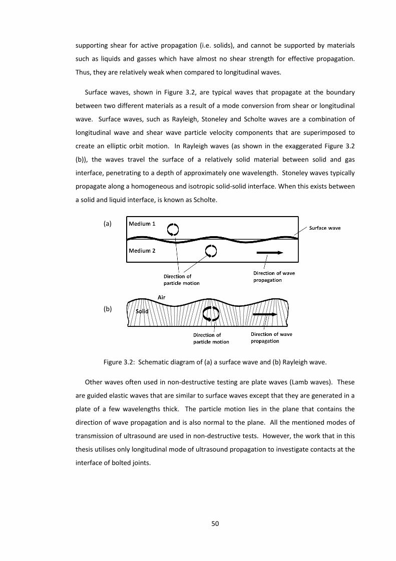
50

supporting shear for active propagation (i.e. solids), and cannot be supported by materials

such as liquids and gasses which have almost no shear strength for effective propagation.

Thus, they are relatively weak when compared to longitudinal waves.

Surface waves, shown in Figure 3.2, are typical waves that propagate at the boundary

between two different materials as a result of a mode conversion from shear or longitudinal

wave. Surface waves, such as Rayleigh, Stoneley and Scholte waves are a combination of

longitudinal wave and shear wave particle velocity components that are superimposed to

create an elliptic orbit motion. In Rayleigh waves (as shown in the exaggerated Figure 3.2

(b)), the waves travel the surface of a relatively solid material between solid and gas

interface, penetrating to a depth of approximately one wavelength. Stoneley waves typically

propagate along a homogeneous and isotropic solid-solid interface. When this exists between

a solid and liquid interface, is known as Scholte.

Figure 3.2: Schematic diagram of (a) a surface wave and (b) Rayleigh wave.

Other waves often used in non-destructive testing are plate waves (Lamb waves). These

are guided elastic waves that are similar to surface waves except that they are generated in a

plate of a few wavelengths thick. The particle motion lies in the plane that contains the

direction of wave propagation and is also normal to the plane. All the mentioned modes of

transmission of ultrasound are used in non-destructive tests. However, the work that in this

thesis utilises only longitudinal mode of ultrasound propagation to investigate contacts at the

interface of bolted joints.

(a)

(b)

51

3.3 Ultrasound and Material Properties

The behaviour of ultrasound in a given material depends on its physical properties. The

stiffness of the material which is a function of its elastic properties affects the speed of

ultrasound while its damping nature will affect the attenuation of sound. The following

subsections explain these characteristic behaviours of ultrasound as related to material

properties.

3.3.1 Speed of sound

The rate at which sound waves propagate in different materials varies. It depends on the

density of a material which is a function of the mass of particles, and also depends on the

relative stiffness of bonding between the particles of a material which is governed by the

elastic constants (bulk modulus, shear modulus or Young modulus) of the material. The

speed of sound in a given material is highest in its solid state and lowest in a gaseous form.

Furthermore, changes in temperature and pressure affect the speed of sound in a gaseous

medium due to their compressibility but this effect is negligible in solids. The speed of sound

is defined as a product of frequency and wavelength, as expressed in the relationship:

𝑐 = 𝑓 3.1

where c is the speed of sound (ms-1), f is the frequency of the sound wave which is equal to

that of the source (Hz) and, is the wavelength (m).

3.3.2 Acoustic impedance of materials

The acoustic impedance of a material is a measurement of its ability to transmit sound.

This is a very important characteristic in ultrasound. It is useful in assessing absorption of

sound in a material, to determine the transmission and reflection of acoustic energy at the

interface of two different materials with different acoustic impedances. It is also essential in

the design of transducers. The acoustic impedance of a given material is defined as a product

of wave speed and density of the material, as given by Equation 3.2.

𝑧 = 𝜌𝑐 3.2

Where z is the acoustic impedance and has a unit of Rayl (Pa.s.m-3), is the density of the

material (kg.m-3).

52

Different materials have a different acoustic impedance. Ultrasound pulse will move

through a material until it encounters a boundary. At the boundary between two perfectly

bonded materials of different acoustic impedance, some of the incident pulse is reflected

back into the first material, while the remainder crosses into the second material (as shown

in Figure 3.3). The amount of the incident pulse that is transmitted and reflected depends

upon the difference between the acoustic impedance of the materials on either side of the

boundary. The larger the impedance mismatch between two media, the smaller the amount

of the ultrasound that will cross the boundary, and the harder to transmit ultrasonic signals

between them.

Figure 3.3: Reflection of ultrasound at the boundary of a perfectly bonded material.

3.3.3 Attenuation

The term attenuation quantifies the reduction in intensity of sound wave energy as it

travels through a material. Attenuation is a function of material properties, frequency and

distance. It is useful in knowing the suitable distance in a material through which the

ultrasound can be transmitted before its energy is too small to be gainfully analysed.

Ultrasonic attenuation, therefore, is the decay rate at which ultrasound wave amplitude

reduces as it propagates through a material, and it is expressed as:

𝐴 = 𝐴0𝑒−𝛼𝑥 3.3

where A and A0 are the attenuated and initial amplitudes of the propagating ultrasound wave

at some distance, x (m) is the distance travelled and (Npm-1) is the attenuation coefficient.

Attenuation is expressed in decibels (dB). Absorption, scattering and radiation are known to

be the major cause of attenuation of ultrasound waves.

(i) Absorption

Ultrasound is said to be “absorbed” by a material if some of its energy is

converted to other forms of energy, thereby reducing its strength as it transmits

53

through the material. This is due to hysteretic losses in the bonding of the

particles of the material as they vibrate about mean positions. Absorption is

frequency dependent; the higher the frequency of the ultrasound wave, the more

the local velocity of vibration of particles of the material at the wavefront, and the

higher the absorption of the ultrasound energy.

(ii) Scattering

Scattering is the non-orderly reflection of sound in directions other than its

original direction of transmission. The change of direction of the sound wave

occurs as a result of discontinuities such as voids, inclusions and grain boundaries

due to the inhomogeneous nature of materials. Scattering occurs when ultrasound

encounters small particles compared to its wavelength, or discontinuities that are

comparably equal to or larger than its wavelength. Since the velocity of sound is a

material property, the higher the frequency of transmission of ultrasound in a

material the lesser the wavelength of the ultrasound and the more it is susceptible

to scattering at the voids and grain boundaries. This is a reason why it is difficult to

transmit ultrasound at a very high frequency in a material with ‘coarse’ grain

boundaries such as cast iron and wood.

(iii) Radiation

The intensity of bulk wave such as a longitudinal wave emitted from a point

source reduces according to the inverse square law as it propagates from the

source. The greater the distance of a point from a sound source in given material,

the lesser the intensity (amplitude) of the sound at the point.

3.4 Production of Ultrasound Waves

Generating ultrasound waves requires repeated mechanical displacement of material

particles about a mean position at a high frequency. To achieve this, a number of different

methods are available and one such method utilises a phenomenon called the piezoelectric

effect. The piezoelectric effect is a behaviour exhibited by some crystalline materials which

involves the reversible conversion of mechanical to electrical energies.

54

3.4.1 Piezoelectric effect

When the crystals of piezoelectric materials (such as quartz) are mechanically compressed

or stretched, they produce a polarised electrical charge at the surface of the material which

depends on the direction of the mechanical stress, and this is known as the piezoelectric

effect. Conversely, piezoelectric crystal responds to the application of potential difference

between its faces by either contracting or expanding, depending on the direction of the

electrical potential difference, and this is known as a reverse piezoelectric effect. Therefore,

the production of ultrasound relies on the reverse piezoelectric effect and the detection is

based on the piezoelectric effect. As a result of this reversibility phenomenon of the

piezoelectric effect, it is possible to use the same piezoelectric crystal to generate ultrasound

waves and also to detect echoes returning to the crystal from a reflector.

3.4.2 Piezoelectric ultrasonic transducers

An ultrasonic transducer is a device used to convert electrical energy into high frequency

sound waves in the ultrasonic range and verse versa. A piezoelectric ultrasonic transducer

contains a piezoelectric plate that vibrates and emits ultrasonic waves when electrical pulses

strike it. As earlier mentioned, the reversibility of the piezoelectric effect allows a

piezoelectric ultrasonic transducer to act as a generator and receiver of ultrasonic signals

separately or as both the generator and receiver in pulse-echo mode. When operating in

pulse-echo mode, the reflected signals from a reflective surface that strike the piezoelectric

plate is converted to electrical voltage and these can be measured and analyse by a data

processing device.

There are many available commercial piezoelectric transducers for various ultrasonic

applications. They are optimised for clarity of signal and specific uses for the different types

of sound wave modes generated. Figure 3.4 (a) shows images of typical commercial

ultrasonic transducers, while Figure 3.4 (b) shows a schematic diagram of a sectioned

longitudinal focused transducer. The piezoelectric element is encased in a sealed housing

with an externally connected wire through which the voltage is conveyed to its electrode.

Attenuative medium (damping material) is placed between the piezoelectric plate and the

housing at the back of the plate to prevent ringing of the housing due to the vibration of the

plate. It also to help suppress the natural resonant oscillation of the plate which will continue

to vibrate for a short period after pulsing.

55

Figure 3.4: (a) Examples of commercial ultrasonic transducers and (b) Schematic

diagram of longitudinal focused ultrasonic transducer.

The thickness of the piezoelectric plate determines the resonant frequency at which the

plate is excited and this dictates the set frequencies of the ultrasonic signal emitted from the

plate upon excitation. The wavelength of the emitted signal is usually twice the plate

thickness when the plate vibrates freely. When the plate is excited, elementary waves are

generated along the length of plate front, which interacts to form a series of propagating

wavefronts. The formation of ultrasound wavefronts from a piezoelectric plate can be

explained using the Huygens’ Principle. According to this principle, every point on a

wavefront may be considered a point source of secondary spherical wavelets that spread out

in the direction with a speed equal to the speed of propagation of the wavelets, and the new

wavefront is the tangential surface to all these secondary wavelets.

Figure 3.5: (a) Radiating spherical wavelets (b) Plane wavefront propagation from

spherical wavelets.

With many spherical wavelets radiating from a transducer as illustrated in Figure 3.5,

many regions of constructive and destructive interference are created in the medium of

propagation. The total pressure in a given region equals the sum of pressures contributed by

each wavelet. The regions are shown as intersections of lines representing compression

zones of individual wavelets. Therefore, the ultrasound wavefront can be viewed as a surface

where the ultrasonic wave has a constant phase due to the combined effect (i.e. total

pressure) created by a series of circular source wavelets.

56

The longitudinal ultrasonic pressure waves formed are then emitted only through the

wear plate (Figure 3.4 (b)) due to the attenuative nature of the material surrounding the

transducer. The piezoelectric plate can be manufactured in many different shapes and sizes.

The wear plate can be profiled so as to provide a focusing effect, thereby concentrating the

sound signal to a particular location similar to the effect of focused light produced by an

optical lens. A longitudinal focused transducer with a circular piezoelectric plate element is

used in the study of static bolted joint in chapter 4 of this thesis.

Commercial transducers, though optimised for signal clarity, have application limitations.

One of these limitations is that they are not easy to couple in a horizontal orientation to

moving specimen. Their usage may also be limited by space constraints, especially when

many transducers are to be used simultaneously within a small confined area. In such a case,

off-the-shelf bare piezoelectric elements (Figure 3.6) are available in a variety of forms that

can be utilised. This type of piezoelectric element was used in many of the experimental

works contained in this thesis to overcome the aforementioned limitations of the commercial

ultrasonic transducers.

Figure 3.6: Examples of off-the-shelf bare piezoelectric elements.

As shown in Figure 3.7, the piezoelectric element discs come in two configurations; the

standard electrode and the wrap-around electrode. The wrap around allows access to both

terminals of the piezoelectric element from one side. This is advantageous because it permits

a strong acoustic coupling and transmission in a situation where one of the surfaces covered

by electrode must be bonded to the test specimen. The piezoelectric elements used in

research works in this thesis have been polarised to provide a through-thickness vibrational

mode when electrically excited. They were also pre-sputtered with wrap around electrodes

of silver. The discs have a centre frequency of 10 MHz, a diameter of 7.1 mm and thickness of

0.2 mm. In some cases during the instrumentation of specimens for the studies, the

piezoelectric element is sometimes modified into a smaller size and different shapes

according to the specimen instrumentation space demands, and also to maximise the

57

resolution of the element. Modifications and operations of the piezoelectric element are

discussed in detail in chapter 6 of this thesis.

Figure 3.7: Schematic diagram of piezoelectric element with (a) standard electrode and

(b) wrap-around electrode configuration.

3.5 Ultrasonic Pulse

Ultrasonic pulse is the wave generated by an ultrasonic transducer in a particular

direction. When a piezoelectric plate in an ultrasonic transducer is excited by a voltage pulse,

it emits an ultrasonic signal containing a range of sound frequencies as it oscillates a number

of times before decaying to zero depending on the degree of coupling and the damping

properties of the transducer. As shown in an example of ultrasonic pulse in the time and

frequency domain in Figure 3.8, the pulse emitted contains a set of frequencies centred over

a dominant frequency (c) which contains the maximum energy, and is called the centre

frequency. As the distance from the centre frequency increases, the energy level of the

frequencies surrounding it decreases. Bandwidth is the term used to classify the useful

frequency range of the transducer. This is the useful frequency range over which information

can be determined about a contact by the transducer. The upper and lower limit of the

bandwidth contains frequencies with amplitude within -6dB of the maximum signal strength

at the centre frequency, and this corresponds to an energy level drop of 50% of the centre

frequency.

Figure 3.8: Example of ultrasonic pulse produced by a transducer shown in a (a) time

and (b) frequency domains.

(a) (b)

58

An undamped transducer produces a large frequency output very close to its centre

frequency, and the amplitude of its response decreases considerably away from the centre

frequency as depicted in Figure 3.9. The damped transducer produces a small output very

close to its centre frequency, but the amplitude of its response decreases slowly at the either

side of its centre frequency. Therefore, damped transducer operates on a broadband of

frequencies and can be driven at a range of frequencies on either side of the centre

frequency. Undamped transducer operates on a narrow broadband and thus, can be best

driven at its centre frequency and small frequency around the centre frequency. Although,

the piezoelectric elements used in some of the research works in this thesis are undamped,

but they are excited at their centre frequency. Therefore, useful information will be obtained

since the signals are generated and acquired at their centre frequency..

Figure 3.9: Frequency response of damped and undamped transducers.

3.6 Ultrasonic Couplant

Sound waves are mechanical vibrations that elastically propagated through a host

medium. For ultrasound to travel through a moving medium, its wavelength must be greater

than the scale of the medium. If a sound wave travels through a medium with fast moving

particles of scale equal to or greater than the sound wavelength, the sound signal is

interrupted by the moving particles, and hence the signal would be broken down, scattered

and lost. Also, when there is a large impedance mismatch between two media, it would be

hard to transmit ultrasonic signals between them (as explained in Section 3.2). Therefore, it is

very difficult to transmit high frequency ultrasonic signals through an air gap between a

transducer and solid as there exists a large impedance mismatch at the solid-air boundary. To

overcome this, ultrasonic couplant is used to transmit signals between the transducer and

specimen. The commonly used couplant are water, oil and gel. Figure 3.10 (a) and (b) show

transducers coupled to a specimen through a gel and water bath respectively. Ultrasonic

“water-immersion” or “water bath” systems are widely used in non-destructive testing. It

59

exhibits an insignificant absorption at low MHz frequencies and generally does not affect the

physical, chemical and mechanical properties of most industrially-important materials. In a

water bath system, the transducer can move over different parts of a scanned sample

without breaking the coupling, this is a significant advantage over gel. As a result of the

advantages, a water bath coupling system was used during the scanning of the static bolted

joint in this thesis.

Figure 3.10: Ultrasonic transducer coupling with (a) gel and (b) water bath.

3.7 Focusing of Transducer

Ultrasonic wave has properties that are similar to that of visible light waves due to the

closeness in the order of magnitude of their wavelengths. Ultrasonic waves can be focused,

reflected and refracted like light waves. When a transducer is excited, it emits a parallel beam

of ultrasound with a diameter equal to that of the piezoelectric plate of the transducer. In

order to increase the sensitivity of a transducer, a concave lens wear plate is sometimes

bonded to the front of the transducer to converge the ultrasonic waves to a focal point as

shown in Figure 3.11 (a). The focal length of a given transducer depends upon the angle of

the lens. The focal length of ultrasonic transducer is difficult to calculate as its focus in not

entirely depends on the lens; the wave interaction as the signal converges also influences the

position of the transducer focus [146]. Nevertheless, the focal point of a transducer can be

calculated in water, and consequently, manufacturers produce ultrasonic transducers of

known focal lengths in water.

In order to investigate an interface, the ultrasonic signal must be focused onto the

interface. Figure 3.11 shows an example of how an ultrasonic signal can be focused onto such

interface. As shown in Figure 3.11(a), a focused ultrasonic transducer converges the

ultrasonic waves to a focal point of a known focal length in water. But, when the transducer is

moved over the specimen, the ultrasound signal is refracted at the boundary as the signal

enters the specimen from the water (as shown in Figure 3.11(b)). Hence, the focal length of

60

the signal changes from that of the water. As ultrasonic signals propagate through two media

it refracted at the boundary of these media in accordance with Snell’s law:

𝑠𝑖𝑛𝜃𝑖

𝑠𝑖𝑛𝜃𝑟=

𝑐1

𝑐2 3.4

where θi and θr are the angles of incidence and refraction r, and c1 and c2 are speeds of

sound in the medium before and after the boundary respectively. Therefore, the water path,

and consequently the transducer position, necessary to focus the ultrasound waves at an

interface, can be calculated since the angles of incidence and refraction are known and also

the thickness of the upper specimen Figure 3.11(b & c).

Figure 3.11: (a) Focal length of converge ultrasonic signal in water (b) Refraction of ultrasonic

signal at H20 and solid boundary, and (c) Focusing of the signal at the solids interface.

3.8 Focused Spot Diameter

The diameter of the finite spot size of the ultrasonic signal when focused on the interface

is known as the focused spot diameter. It qualifies the resolution of the ultrasonic technique,

and is quantified in terms of the bandwidth:

Spot diameter (-6 dB) =1.025𝑙𝑤𝑐𝑤

𝑓𝑑𝑐 3.5

where f, dc, lw and cw is the frequency, the diameter of the piezo-crystal, the focal length and

the speed of sound of transducer respectively.

A very small, focused, ultrasonic spot is always desirable as it improves the resolution of

the technique. Equation 3.5 shows that the higher the centre frequency of the ultrasonic

transducer the smaller the spot diameter. Therefore, it is appropriate to maximise the centre

frequency of the focused transducer when investigating an interface at a set distance.

However, the higher the centre frequency of a transducer, the smaller the wavelength of the

ultrasound produced, the more susceptible is the ultrasonic signal to attenuation due to

absorption and scattering at the grain boundary (Section 3.2.3). Subsequently, applying

61

ultrasound with too high a frequency may lead to loss of the entire signal before reaching the

focused interface or when returning from the interface. Therefore, when selecting a

transducer for the purpose of investigating an interface ultrasonically, it is good to select a

transducer with a centre frequency that will maximise resolution of the technique whilst

ensuring that the signal is not lost as it travels to and from the interface in the material

specimen. The transducer used for the investigation of the contact pressure at the interface

of a bolted joint was purchased from NDT Systems Inc. Table 3.1 shows the specifications for

the transducer.

Table 3.1 Specification of ultrasonic transducer

Nominal frequency

(MHz)

Focal length in water (mm)

Centre frequency

(MHz)

Bandwidth (MHz)

Focused spot diameter

(mm)

10 76 8.8 4.5 0.9

3.9 Ultrasonic Reflection at Rough Surface Contacts and the

Spring Model

Contacts in engineering surfaces are non-conformal. They exhibit surface roughness,

which is manifested in the form of surface waviness and asperities, and this is evident when

observed under the microscope [147]. Therefore, when two engineering surfaces, especially

metals, are bolted together they mostly interact at the junctions of the surface

roughness/asperities, with air gaps at the void between the asperities. Figure 3.12 shows a

schematic diagram of loaded rough surfaces in contact.

Figure 3.12: Real surfaces in contact.

When an ultrasonic wave encounters an interface between materials of different acoustic

properties normal to its direction of travel, the energy within the acoustic wave is partially

62

transmitted into the second material while the remainder is reflected back in the opposite

direction of initial travel. Therefore, when normal ultrasound waves are incident on a

contacting interface, such as in bolted joints, the sound waves are partially reflected at the

interface (as shown in Figure 3.13). The reflection is at the metal-air interface due to the

trapped air pockets, with sound transmitted at the asperity junctions. How much sound is

transmitted depends on the wavelength of the sound wave relative to the air gap.

Figure 3.13: Ultrasonic reflection at rough surface interface.

The proportion of the ultrasound wave incident on the interface that is reflected from it is

known as reflection coefficient for displacement wave amplitude, R, and is given as:

𝑅 =𝑧1−𝑧2

𝑧1+𝑧2 3.6

where z is the acoustic impedance and, subscripts 1 and 2 refer to acoustic impedance for the

material on either side of the interface. The acoustic impedance is equal to product of wave

speed and density for a given material (according to equation 3.2).

In a study conducted by Kendall and Tabor [148] on rough surface contacts, the asperity

interactions of the interface were modelled as a series of parallel springs (Figure 3.14). This

was also followed up by Tattersall [149] on adhesive layers. They found out that the

reflection coefficient depends on the interfacial stiffness, K, and is given by:

𝑅 =𝑧1−𝑧2+𝑖𝜔(𝑧1𝑧2/𝐾)

𝑧1+𝑧2+𝑖𝜔(𝑧1𝑧2/𝐾) 3.7

The modulus of the reflection coefficient is given as:

|𝑅| = √(𝜔𝑧1𝑧2)2+𝐾2(𝑧1−𝑧2)2

(𝜔𝑧1𝑧2)2+𝐾2(𝑧1+𝑧2)2 3.8

For homogenous contact with two similar materials, the relationship between the

reflection coefficient and the interfacial stiffness is reduced and governed by:

|𝑅| =1

√1+(2𝐾 𝜔𝑧⁄ )2 3.9

63

where is the angular frequency which is equal to 2f.

Figure 3.14: Schematic representation of an interface using the spring model.

Experimental studies conducted by Drinkwater et al. [150] on the spring model showed

that the model can be applied to ultrasonic reflection data from rough surface contacts for

ultrasound frequencies up to a maximum of 50 MHz, depending on the materials and surface

roughness of the contact under investigation.

3.10 Interfacial Stiffness and Contact Pressure Measurement

The interfacial stiffness, which is expressed per unit area, is defined as the change in nominal

contact pressure, Pnom, required to cause unit approach of the mean lines of two surfaces.

𝐾 = −𝑑𝑃𝑛𝑜𝑚

𝑑𝑢 3.10

where u is the separation of the mean lines of roughness of the two surfaces.

Interfacial stiffness for a given pair of contacting surfaces varies from zero when the

surfaces are just touching (the asperities can easily be deformed and separation between

surfaces can be reduced) to infinity when surfaces are completely conformal (when

deformation of the asperities and reduction of separation between the surfaces is no longer

possible). The interfacial stiffness also depends on the distribution, size and number of

asperity junctions. Thus, its value is partially linear and depends on applied load, with no

single relation between it and contact pressure.

In investigating this problem, Dwyer-Joyce and Drinkwater [151] determined that a

relationship could to be established between the contact pressure and the interfacial

stiffness through a calibration experiment. Subsequently, this method provides the

opportunity to obtain a contact pressure distribution from a map of the ultrasonic reflection

from an interface. An experimental study conducted on the spring model by Drinkwater et al.

64

[150] showed that the model could be applied to reflection data from rough surface

interfaces for ultrasound frequencies up to a maximum of 50 MHz, depending on the

materials and surface roughness of the contact surfaces under investigation. Studies carried

out by Arakawa [152] and Hodgson et al. [153] showed that at low applied loads the relation

between the contact pressure and interfacial stiffness is linearly proportional.

3.11 Ultrasonic Apparatus

In order to carry out research works using ultrasonic techniques stated in this thesis,

appropriate electrical hardware were essential to generate, capture, display and record the

ultrasonic signal. To achieve all these, a self-contained ultrasonic pulsing hardware unit

(FMS100 PC System) that accommodates all the components that could accomplish the

mentioned requirements was used. Each component of the ultrasonic hardware unit could

be configured, thereby giving a very versatile system, which could be modified to suit the

requirement for each of the intended experimental works. Figure 3.15 shows a schematic

diagram of the ultrasonic pulsing apparatus.

Figure 3.15: Schematic diagram of ultrasonic pulsing apparatus.

The core unit of the ultrasonic pulsing apparatus is the ultrasonic pulser-receiver (UPR)

which comprises of the ultrasonic pulser and the ultrasonic receiver. The pulser component

generates a high-frequency voltage pulse that is used to excite the piezoelectric element. This

component contains a PCI card (built by Tribosonic/NDT Solutions Ltd) with 8 channels that

could be configured individually, enabling different transducers to be excited as required. It

has a total pulse rate that could be varied from 60 to 80,000 pulse/second, split across

channels that were active during operation. The pulse voltage could be varied from 5V to

approximately 300V while the centre frequency could be varied from 1 to 20 MHz.

The receiver component received the high-frequency voltage of the converted reflected

ultrasonic signal from the piezoelectric element. The receiver component was also a PCI from

65

the same manufacturer as the pulser. It has 8 channels that could equally be configured

individually to enhance the performance of the ultrasonic system. Each of the channels could

be configured to recognise the waveform of interest through a ‘Window’ containing an

individual reflection. A delay and range could be set to move the window in time to centre it

on the reflection of interest, limiting the volume of signal content which would be passed for

storage and processing.

As mentioned above, the UPR system has a capacity of running up to 8 channels at a time

with one transducer connected to each channel. If more than eight multiple transducers are

required, then a multiplexer unit of the ultrasonic pulsing apparatus is used as an automatic

‘changeover’ between the transducers with a maximum of eight transducers active at a time.

When in operation, as the 8 channels are continuously pulsed by the UPR, the signals from

these channels are transmitted to the multiplexer unit. Then, the multiplexer sequentially

distributes these signals to the transducers, and the reflected signals return to the UPR in the

reverse order. The multiplexer unit sends and receives signals from 8 transducers at a time

and can distribute the signals sequentially between 64 sensors at a switching frequency of up

to 10 Hz. The features and operation of the multiplexer unit are discussed in detail in Chapter

6.

The operation of the pulsing apparatus is built around the PC, upon which a commercially

available software package is installed to control all the units. The PC sends a controlled

signal that triggers the pulser unit to generate a high-frequency voltage pulse. The voltage

pulse is used to actuate the piezoelectric plate of the transducer, which converts the

electrical excitations to ultrasonic signals that are consequently emitted to the targeted

contact interface. The reflected ultrasonic signals from the interface strike the piezoelectric

plate. Since the plate is a reciprocal element, it converts the motion of the ultrasound wave

to a high-frequency voltage. The voltage was then passed to the receiver unit for onward

transfer to the digitizer where the reflections were sampled at a resolution of 12 bits and at a

rate of 100 million samples/second. The PC displays both the emitted and reflected signals.

3.12 Scanning Apparatus

The scanning apparatus (also known as the scanning tank equipment) along with the

ultrasonic pulsing unit used in the study of the contact pressure distribution in the interface

of bolted joints, in chapter 4, is shown in Figure 3.16. An immersion water tank was

constructed on the scanning tank bed of the apparatus. However, for the purpose of clarity,

the immersion water tank has been removed. The specimen under investigation is immersed

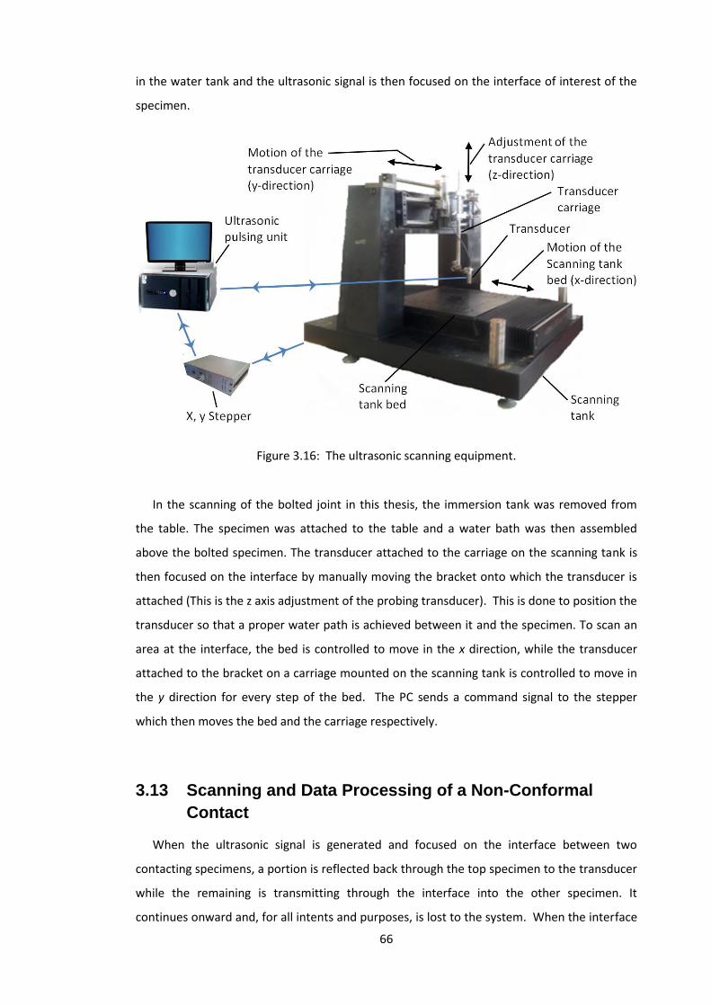
66

in the water tank and the ultrasonic signal is then focused on the interface of interest of the

specimen.

Figure 3.16: The ultrasonic scanning equipment.

In the scanning of the bolted joint in this thesis, the immersion tank was removed from

the table. The specimen was attached to the table and a water bath was then assembled

above the bolted specimen. The transducer attached to the carriage on the scanning tank is

then focused on the interface by manually moving the bracket onto which the transducer is

attached (This is the z axis adjustment of the probing transducer). This is done to position the

transducer so that a proper water path is achieved between it and the specimen. To scan an

area at the interface, the bed is controlled to move in the x direction, while the transducer

attached to the bracket on a carriage mounted on the scanning tank is controlled to move in

the y direction for every step of the bed. The PC sends a command signal to the stepper

which then moves the bed and the carriage respectively.

3.13 Scanning and Data Processing of a Non-Conformal

Contact

When the ultrasonic signal is generated and focused on the interface between two

contacting specimens, a portion is reflected back through the top specimen to the transducer

while the remaining is transmitting through the interface into the other specimen. It

continues onward and, for all intents and purposes, is lost to the system. When the interface

67

is separated and there exists a complete steel-air interface, the ultrasonic signal is completely

reflected back to the transducer because of a large impedance mismatch that occurs at the

steel-air boundary as discussed in Section 3.8. For example, Figure 3.17 shows a schematic

diagram of two specimens when loaded together and when the lower specimen has been

removed for reference measurement. The reference scanning is carried out in order to

create a metal-air interface so that the entire ultrasonic signal will be reflected. For example,

the transducer was focused at the loaded interface and scan was then performed over 5 mm

5 mm contact area. The amplitude of the reflected ultrasonic pulse was measured at every

0.25 mm 0.25 mm.

Figure 3.17: (a) Scanning of loaded interface; (b) A reference scan.

Figure 3.18 shows an example of a measured reflected pulse from the interface, isolated

in the time domain. The reflected signal in the figure represents the measured reflected pulse

for the loaded specimens, while the reference signal represents the reflected pulse for the

reference measurement. The reflected signal from the loaded interface has a lower value

because there was partial transmission of the signal at the interface, and also as a result

attenuation that occurred in the material bulk of the upper specimen. The reference

measurement was performed to quantify the attenuation of the ultrasonic signal as it travels

to and from the interface in the bulk material of the specimen, and this is required for the

calculation of the reflection coefficient.

Figure 3.18: Example of measured reflections from the scanned interfaces in time domain.

68

Since the peaks of both the reflected voltage and the reference voltage signals are at the

centre frequency of the applied transducer, the reflection coefficient is calculated by dividing

the amplitude of the reflected voltage by the amplitude of the reference voltage. By doing

this, attenuation is cancelled out in the material bulk, leaving only the fraction of the total

ultrasound incident on the interface that is reflected back.

The map of the reflection coefficient of the scanned interface is produced by dividing the

reflected voltage of the scan interface with the corresponding scan of the reference voltage.

Since the two scans are produced over the same area at the same resolution, it implies that

the reflected voltage at each point on the interface is divided by its corresponding reference.

The spring model (discussed in Section 3.8) is then applied to the map of reflection coefficient

to produce the map of interfacial stiffness according to equation 3.9.

The technique discussed so far is the time domain method. It is also possible to analyse

ultrasonic reflection data in the frequency domain [150]. In the time domain method, the

assumption is made that the peak amplitude of both the incident and reflected pulses occur

at the centre frequency of the transducer [150]. While in the frequency domain method,

reference and reflected signals for each given point in the scan are completely downloaded

to the PC, and then converted to the frequency domain using a Fast Fourier Transform (FFT).

As illustrated in Figure 3.19, the reflected FFT and reference FFT is then used to determine

the reflection coefficient and then the interfacial stiffness over the frequency range of the

transducer.

Figure 3.19: Example of a point measured ultrasonic reflections within the scanned area

in a frequency domain.

69

The spring model is applied to the reflection data over the bandwidth (which is the

frequency range over which useful information about the contact can be determined) of the

transducer to determine the interfacial stiffness. The interfacial stiffness is independent of

frequency and can be obtained from the calculated data [150]. If the frequency domain

method is, therefore, to be used, it implies that the process of downloading complete

waveforms for both reference and reflected signals must be repeated for every point in the

scan. In reality, this would be time consuming, especially where scans of large interfaces are

to be performed. However, the time domain method represents a substantial time saving

when repeatedly scanning a large contact when compared to the frequency domain method,

and this is the technique that would be applied in the scanning of the bolted joints.

3.14 Calibration Experiment for Contact Pressure

To find the relationship between interfacial stiffness and contact pressure at the interface

of a bolted joint specimen, a calibration experiment needs to be performed. The calibration

specimens are manufactured from the same material and given a similar surface treatment as

that of the bolted specimen. Figure 3.20 (a) shows a schematic diagram of the calibration

experiment set-up with the loaded specimens used in the calibration experiment. The

specimens are loaded together and single-point reflections of the contact interface are

recorded for a series of known loads. The reference measurement is also recorded with the

lower specimen absent (steel-air interface). The reflection coefficient and the Interfacial

stiffness are then calculated for the different loads applied as discussed in section 3.13. Since

the contact area of the specimens is known, the contact pressure at each load can be

calculated for the different loads. A plot of the calculated contact pressure against the

corresponding interfacial stiffness can then be produced. An example of this type of graph

produced by Marshall et al. [44] is shown in Figure 3.20 (b).

70

Figure 3.20: Example of (a) calibration experiment set-up and (b) graph of the interfacial

stiffness versus contact pressure [44].

3.15 Monitoring of the Relaxation of Contact Interface under

Dynamic Load

The technique described so far is for the scanning of the interface of static bolted joints. A

different ultrasonic technique was used for monitoring the relaxation of bolted joints in

Chapter 6, shear of an adhered interface in Chapter 7, and monitoring of relaxation of both

insulated block joints and a temporary rail joint in chapter 8. Although the theoretical

principle is the same as that of the scanning of the bolted joint, the technique involves

bonding of a piezoelectric sensor (element) directly to the specimens. When the sensor is

pulsed, it produces a slightly diverge longitudinal ultrasound wave approximately equal to the

size of the sensor. Therefore, the resolution of this technique depends on the size of the

piezoelectric sensor used.

Figure 3.21 (a) shows an example of bolted components subjected to dynamic shear

loading. When the piezoelectric sensor is pulsed, the longitudinal ultrasound signal incident

on the bolted interface is partially reflected at the material-air junctions and partially

transmitted across the interface at the asperity junctions of the contact interface. However,

as the surfaces of the components (plate A and plate B) that make up the bolted interface

separates, the number of the asperity junctions decreases and thus, the quantity of reflected

signal from the interface increases until there is complete separation of the surfaces leading

to total reflection of the signal at the interface.

71

Figure 3.21: Example of (a) monitoring of dynamic loaded interface and (b) graph of the

dynamic reflection of the interface.

If the reference signal is taken initially when the plates are separated before tightened,

the reflection coefficient can be calculated by dividing the reflected signal during the

separation of the bolted components with the reference signal. By doing this, the attenuation

of signals in the plate material is cancelled out leaving only the fraction of the total

ultrasound incident on the interface that is reflected back. Since the quantity of reflected

signal from the interface increases as the surfaces that make up the interface separate.

Therefore, the calculated value of the reflection coefficient of the interface changes with time

as separation occurs.

Figure 3.21 (b) shows an example of the dynamic reflection coefficient calculated from the

separating interface due to dynamic shear loading. When the value of dynamic reflection

coefficient is less than 1, it indicates that the bolted plates are in contact. As the value

increases towards 1, the contact between the interface of the plates decreases, which implies

that the plates are separating. A value of 1 indicates that the entire ultrasonic signal has

been reflected from the interface because the plates have separated and the contact at the

interface has become zero. However, if the reference signal is taken when the surfaces are

already clamped, (as obtained in the case of the adhesive bonded interface in chapters 7 and

8), the value of the dynamic reflection coefficient increases from a value of 1 to a maximum

value when the surfaces separate. Therefore, in all cases, an increase in the value of the

dynamic reflection coefficient signifies separation of contact surfaces.

3.16 Conclusions

Ultrasound is a general term used to describe mechanical pressure waves that propagate

at frequencies above the range of human hearing, and ultrasonic is the application of

72

ultrasound waves. The behaviour of ultrasound in a host material depends on the physical

properties of the material. Ultrasound can be generated in a variety of different methods,

and one such method utilises a controllable piezoelectric effect exhibited by some crystalline

materials. When a voltage is applied to a piezoelectric material it deforms and emits

ultrasound, and when subjected to mechanical strain from ultrasound, it generates a voltage.

Therefore, it can be used as both the emitter and receiver of ultrasound.

A longitudinal wave is one mode of transmission of ultrasonic waves, and can propagate in

both solids and liquids. Hence, it can be used in ultrasonic tests that involve most engineering

materials. However, a couplant is required between the ultrasonic transducer (source) and

mechanical component (target) to effectively transmit an ultrasound wave between them.

Water is a good couplant that can be used, especially when the transducer scans over the

component. Models exist to describe the behaviour of ultrasonic waves at medium

boundaries. When the ultrasonic wave is incident on an interface between two components,

the wave is partially transmitted and partially reflected.

Furthermore, the reflection of the ultrasonic wave can be acquired and processed to

obtain information about the nature of the contact at the interface. The reflection is used to

calculate the reflection coefficient of the incident wave at the interface. The calculated

reflection coefficient can then be processed using the spring model to obtain a map of the

interfacial stiffness of the contact interface. The relationship between the interfacial contact

and the contact pressure at a loaded interface can be obtained through a calibration

experiments. This relationship, along with the map of the interfacial stiffness, can then be

used to obtain the map of the contact pressure distribution of the loaded contact interface.

Ultrasound can be applied to monitor a separating interface, such as the loosening of a

bolted joint subjected to a shear loading. When ultrasound is used for this purpose, the

reflection coefficient obtained is dynamic, and the value of the dynamic reflection coefficient

will increase to signify the separation of contact surfaces.

73

Chapter 4 Ultrasonic Scanning of a Static Bolted Joint

Ultrasonic Scanning of a Static Bolted Joint

4. Bolted joints are known to associate with a number of advantages when correctly

selected. Their clamping performance and the stiffness depends on quantitative

representation of the contact pressure distribution at the interface during design.

Because of the difficulty in reaching and assessing clamped interfaces with traditional

experimental methods, presently bolted joint design and evaluation is based on

theoretical analysis, with assumptions to quantify pressure distribution at the

clamped interface, which may not represent their true operating conditions. In this

chapter, a non-intrusive ultrasonic technique was utilised to investigate and quantify

the pressure distribution in bolted joints. Firstly, the effect of variation in plate

thickness on the contact pressure distribution at bolted interfaces under varying axial

loads was investigated. While in the second part of this chapter, the effect of

variation in bolt head on the contact pressure distribution at the bolted interface

under varying axial loads was also examined. This was to verify the facts established

through theoretical and numerical models, and also provide additional information to

the body of knowledge regarding the contact pressure distribution in bolted joints

which will be beneficial to the design of bolted joints.

4.1 Introduction

Bolted joints are widely used in modern engineering structures and machine design due to

their high load-carrying capacity and reliability when correctly selected, ease of assembly and

disassembly of structures/machine components (especially for maintenance purposes), and

relatively low cost and efficient manufacturing process [154]. As a brief recap of the earlier

discussions under the literature review, many of the investigations carried out have been

focused on the integrity (i.e. the clamping performance and stiffness) of bolted joints as a

function of their stiffness and response to loading and, in some cases, ability to conduct

thermal energy at the joints. The geometry and the magnitude of the contact pressure

distribution at the clamped interface have been extensively discussed by most of these

studies [13, 29, 35, 37, 38, 40, 155]. The contact pressure distribution is important when

calculating the clamping performance of the bolt, and thus the joint stiffness. It is also

74

important when assessing the fatigue life of the joints [13] and also their ability to conduct

thermal energy at the joints [156, 157].

In order to assess the contact pressure distribution at the interface of bolted joints,

analytical models have been developed to predict the pressure distribution in bolted joints as

a function of the contact radius, plate thickness and the bolt head radius [29, 35]. Numerical

models from finite element method have also been used to investigate the pressure

distribution in both single plate and two plate models [37, 38]. Assumptions such as taking

the two plates of the bolted joint as a single plate of identical materials and thickness, which

is equal to the combined thicknesses, are critical issues with the analytical models.

Simplification of external load conditions, bolt geometry and coefficient of friction estimation

at the joint are issues that make determination of contact pressure distribution using the

finite element method very complicated.

Furthermore, in order to develop an experimental technique for determining the contact

pressure distribution at the bolted interface and also to verify the numerical models,

experimental techniques such as coating one of the contacting surfaces of the bolted joint

with radioactive material which were later exposed to radiographic film and developed after

the load had been applied to the joint [37], placing pressure sensitive films between the

loaded contacting surfaces and use of sensitive pin have been employed to determine the

contact stress at the interface of the bolted joints [40, 45]. While results from these

investigations show the contact pressure geometries in the bolted joints, the issue of contact

pressure modification due the insertions between the clamped components of the bolted

joints is of major concerns [40].

Non-intrusive ultrasonic techniques have also been used by different authors [40-44, 65]

to investigate features of bolted joints. More recently among them were the research works

by Pau and Baldi, and Baldi et al. [41, 43] that investigated the pressure distribution in bolted

joints using plates of different thickness. The results of the pressure map and contact

pressure distributions were compared with results from sensitive pressure films and finite

element methods. Although plates of different thickness were tested, the relationship

between plate thickness and interface pressure distribution is not discussed, due to the focus

of the work being the aforementioned comparison of different investigative techniques.

Marshall et al. [44, 65] in their investigation studied bolted surfaces with no washer, plain

and spring washers for a series of different bolt torques using two different interfaces. They

found out that surface profile and washers affect the pressure distribution. They also found

the peak contact pressure occurred at points away from the bolt hole.

75

The results from the ultrasonic techniques clearly showed that this is a good technique

that can be used to study the contact pressure distribution at the bolted joint interface

without intrusion into the contact interface. Therefore, the present study intends to advance

the works in this area by using the ultrasonic non-intrusive technique to study the effect of

variation in plate thickness and diameter of the bolt head on the contact pressure

distribution at the bolted interface under varying axial loads. This is to verify the facts

established through numerical models, and also provide additional information to the body of

knowledge regarding the contact pressure distribution in bolted joints which will be a

valuable tool for evaluating the integrity of bolted joints and also beneficial to the design of

bolted joints.

4.2 Experimental Procedures

Contacts in bolted joints like in other engineering surfaces are non-conformal. They exhibit

surface roughness, which is manifested in the form of surface waviness and asperities.

Therefore, when two surfaces of the bolted joint are loaded together they mostly interact at

the junctions of the surface roughness/asperities, with air gaps at the void between the

asperities. As mentioned earlier in this thesis, when normal ultrasound waves are incident at

the joint interface, the sound waves are transmitted at the asperity junctions, and reflected

at the metal-air interface due to the trapped air pockets. The reflection coefficient is the

fraction of the ultrasonic signal incident at the interface, and this is used to calculate and

produce the map of interfacial stiffness at the interface. The map of interfacial stiffness is

then used along with the result of a calibration experiment to produce the map of contact

pressure distribution at the clamped interface.

Therefore, ultrasonic study of bolted joints in this context is about mapping of contact

pressure distribution at the clamped interface as a function of the reflection coefficient of

ultrasound waves from the interface. Consequently, in order to carry out a qualitative

mapping of the contact pressure distribution at the interface of the bolted joint using

ultrasonic technique, the signal from a focused transducer must be coupled to the test bolted

specimen and transmitted to the interface of interest. This signal must be made to explore a

planned area at the interface. Hence, the specimen must be located properly, and the

focused transducer must be immersed in a couplant and positioned so that the signal only

travels to the interface of interest. The transducer also must be moved by a system so that

the signal travels to points of interest all over the planned area at the contact interface. The

following subsections explain how this was accomplished.

76

4.2.1 Scanning tank equipment

The ultrasonic equipment used consists of a 10 MHz longitudinal focused immersion

transducer which is pulse-echo type. It has a nominal focal length of 76.20 mm in water and

piezo-element diameter of 8.90 mm. It has a centre frequency of 8.8 MHz, bandwidth of 5.5

MHz. Other parts of the equipment include the x, y steppers and PC (FMS100 System).

Schematic diagram of the equipment set-up is shown in Figure 4.1.

Figure 4.1: Schematic Diagram of Ultrasonic Equipment.

The transducer is mounted on the scanning tank and moved over the scanned area by the

steppers. The movement of the steppers is controlled by the PC. The PC sends controlled

electrical excitations to the piezoelectric element in the transducer, which converts the

electrical excitations to ultrasonic signals that are consequently emitted to the targeted

contact interface. The reflected ultrasonic signals from the interface are received and

converted to electrical signals in the transducer, and then passed to the same PC. The PC

displays both the emitted and reflected signals. The reflected signals are stored in the PC for

further processing. The whole process of the scanning is controlled with a programme

written in LabVIEW.

4.3 Static Scanning of Bolted Joints with Varying Plate

Thickness

4.3.1 Test specimens

The bolted joints used in this study consist of steel plates made from EN24 steel and

clamped together with a steel bolt M16 (grade 8.8) bolt as shown in the Figure 4.2. The base

plate was 12 mm thick while the upper plates were 5, 10 and 20 mm in thickness. The plates

were of the same materials so that the contact would be homogenous and there would be no

acoustic mismatch of impedance at the asperity junctions in the contact zone. Clearance

77

holes were drilled through the upper plates to accommodate the bolt. The hole in the base

plate was blind tapped. The contact surfaces of the plates were ground to an average surface

roughness of about 0.5 m (Ra).

Figure 4.2: (a) Diagram of bolted joint specimens showing side and plan views and (b)

Photograph of the Bolted joint.

4.3.2 Scanning procedure

The scanning was performed on a square area of 40 mm 40 mm in the case of the 5 and

10 mm upper plates, and in order to capture a wider contact area a 55 mm 55 mm square

area was scanned in the case of the 20 mm upper plate thickness (as shown by the dotted

line on the bolted joint in Figures 4.3 (a)). The bolt hole was positioned to be at the centre of

the scan in all cases. In order to perform the scans on the loaded joint, the bolted joint

specimens were first assembled with the upper plate in position and torqued up to the

required load using a digital torque wrench with a calibrated accuracy of 2%. The assembled

specimens were mounted on a locating fixture attached to the bed of the scanning tank with

the lower plate facing upwards as shown in Figures 4.3 (b).

As shown in these figures, a water bath was assembled above the bolted specimens, and

the transducer attached to the scanning tank was mounted at appropriate height so as to

focus the ultrasonic signal on the interface of interest according to the explanation given in

Section 3.7 in Chapter 3. The transducer was coupled to the specimens via a deionised water

78

bath mounted on the specimen. Deionised water was used to remove air from the water,

which can scatter and weaken the ultrasonic signal. The water path (height of the transducer

from the top surface of the upper plate) is calculated using Equation 3.4. With the specimens

and transducer in place, the scanning was initiated. The bed is controlled to move in the x

direction with 0.25 mm steps, while the transducer attached to a bracket on a carriage

mounted on the scanning tank was controlled to move in the y direction with 0.125 mm steps

for every step of the bed. This implies that the amplitude of the reflected ultrasound pulse is

measured at every 0.25 0.125 mm. Figure 4.4 shows the experimental setup of the scanning

procedure.

Figure 4.3: (a) Bolted joint with mark to show the scan area at the bolted interface, (b)

Stages of experimental setup.

Figure 4.4: Experimental setup of the scanning process.

79

As earlier mentioned in chapter 3 of this thesis, it is possible to analyse ultrasonic

reflection data either in the time domain or in the frequency domain. The advantage of the

time domain method is that it represents a substantial time saving when repeatedly scanning

a large contact as compare to the frequency domain method. In the time domain method,

the assumption made is that the peak amplitude of both the incident and reflected pulses

occur at the centre frequency. The interfacial stiffness is independent of frequency, and can

be obtained by applying the spring model to the reflection coefficient over the bandwidth of

the probe to determine the interfacial stiffness in the frequency domain method. Hence, the

spring model can be applied to the reflection coefficient obtained from the time domain

method since reflections are assumed to be measured at the centre frequency.

An ultrasonic pulse is generated through a control voltage signal sent by the PC to the

transducer. The signal is focused on the contact surface and reflected voltage from this

surface is received and stored by the PC through the transducer. The voltage of the received

signal is usually smaller than that of the pulse signal, because of attenuation in the material

as the signal travels to and from the contact interface in both scanning procedures, and also

transmission at the asperities junctions in the case of the loaded joint scan. A reference scan

was also performed with the upper plate absent in order to create a metal-air interface so

that the entire ultrasonic signal was reflected. The reflection coefficient is obtained by

dividing the reflected voltage of the loaded joint with that of the reference. By doing this

effect of attenuation is removed, leaving only the map of reflection coefficient for the contact

interface, which represents the fraction of ultrasound incidence at the interface that is

reflected from it. The experimental setup for the scanning of both reference and loaded

bolted joints are shown in Figure 4.5.

Figure 4.5: Ultrasonic scanning of specimen. (a) Reference scan (b) Loaded joint scan.

80

Previously, a limit was highlighted with respect to using ultrasonic scanning on small

surfaces with rapid changes of contact pressure gradient [43, 44]. In this study a focusing

transducer was selected, keeping in mind the attenuation problem associated with higher

frequencies, and was applied on a large surface with gradual changes in pressure, limiting the

effect of smoothing within the ultrasonic focused spot. Although, in order to capture more

details at the bolted interface, the amplitude of the reflected ultrasound pulse was measured

at every 0.25 0.125 mm and a substantial area was recorded. Like other ultrasonic

techniques, it is also limited by the resolution and focused spot size of the transducer used.

4.4 Calibration

The calibration experiment follows the technique stated by Marshall et al. [44] to find the

linear relationship between the stiffness and contact pressure. Additional cylindrical

calibration specimens were made from the same material and subjected to the same surface

treatment as that of the experimental plates. The specimens were loaded as shown in Figure

4.6, and single-point reflections of the contact interface were recorded for a series of loads.

The reference measurement was also recorded with the lower specimen absent. This

reference measurement was used to divide the reflected signals to get the reflection

coefficient at each of the different loads applied.

Figure 4.6: Calibration experimental set-up.

Interfacial stiffness at each load was then calculated from the reflection coefficients.

Since the contact area of the specimens was known, the contact pressure at each load could

be calculated and plotted against the corresponding interfacial stiffness, as shown in Figure

4.7. The same specimens used in Marshall et al. [44] were used, and from the calibration

experiment, the value of m (which is the inverse of the gradient of the least square fit line

that relates contact pressure to the interfacial stiffness) was found to be 61.2. The units of m

are MPa/[GPa/m].

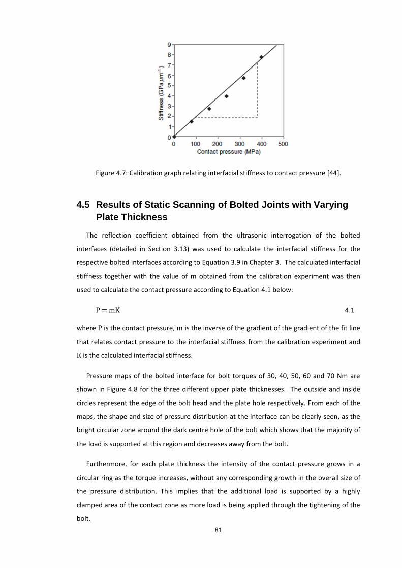
81

Figure 4.7: Calibration graph relating interfacial stiffness to contact pressure [44].

4.5 Results of Static Scanning of Bolted Joints with Varying

Plate Thickness

The reflection coefficient obtained from the ultrasonic interrogation of the bolted

interfaces (detailed in Section 3.13) was used to calculate the interfacial stiffness for the

respective bolted interfaces according to Equation 3.9 in Chapter 3. The calculated interfacial

stiffness together with the value of m obtained from the calibration experiment was then

used to calculate the contact pressure according to Equation 4.1 below:

P = mK 4.1

where P is the contact pressure, m is the inverse of the gradient of the gradient of the fit line

that relates contact pressure to the interfacial stiffness from the calibration experiment and

K is the calculated interfacial stiffness.

Pressure maps of the bolted interface for bolt torques of 30, 40, 50, 60 and 70 Nm are

shown in Figure 4.8 for the three different upper plate thicknesses. The outside and inside

circles represent the edge of the bolt head and the plate hole respectively. From each of the

maps, the shape and size of pressure distribution at the interface can be clearly seen, as the

bright circular zone around the dark centre hole of the bolt which shows that the majority of

the load is supported at this region and decreases away from the bolt.

Furthermore, for each plate thickness the intensity of the contact pressure grows in a

circular ring as the torque increases, without any corresponding growth in the overall size of

the pressure distribution. This implies that the additional load is supported by a highly

clamped area of the contact zone as more load is being applied through the tightening of the

bolt.

82

Figure 4.8: Contact pressure maps of bolted joint at different torques.

83

Figure 4.9: Contact pressure distribution of the plate 5 mm (a) 3D representation and (b) through the vertical section A-A..

Figure 4.10: Surface profiles of (a) section A-A and (b) section B-B.

The pressure distribution is not symmetrically uniform around the centre hole at the

interface. This is due to the effect of non-uniform clamp from the bolt head as a result of the

helix profile of the bolt thread and also from the plate profile irregularities of the contact

(a) (b)

84

surfaces. This effect is shown in Figure 4.9 for the contact pressure distribution of the 5 mm

thickness plate at a torque of 30 Nm. Furthermore, the maximum contact pressure is away

from the edge of the bolt hole, and this is in agreement with observations from earlier study

by Marshall et al. [44]. As shown in Figure 4.9, there are some observed spikes of pressure

recorded inside the bolt hole. This is unexpected as there was no contact of surfaces at the

bottom of the bolt hole, and the ultrasonic signal was not focused in this region. Thus the

observed effect is likely due to scattering from the rough surface of the blind tapped hole,

and since this is not a genuine measurement of contact, has been disregarded.

The patterns of irregularities of the contact surfaces (Figure 4.8) can be seen in the

background away from the circular region of the high contact pressure. Figure 4.10 shows

the Talysurf measured surface profiles, with the Ry (maximum peak-to-valley height) values,

of the 20 mm thick plate taken at section A-A and section B-B. As shown, the contact

pressure in the background region follows the trend of the surface profiles (waviness effect)

at these sections. The pattern is unique for each plate interface, and individual to each of the

plates.

Furthermore, it can be observed that there is a ring of high pressure intensity immediately

inside the minor diameter of the threaded bolt hole. This is evident in Figure 4.9, and also

highlighted in Figure 4.11. This is also unexpected as no reflection of ultrasonic signal is

expected because there is no normal line of sight to this area. This reflection and associated

pressure is attributable to blurring and attenuation of signals, due to scattering effects as the

threads undergo high stress and elastic deformations under loading, at the point where the

inside of the bolt thread comes in contact with the thread of the plate and also focused by

the ultrasonic signal (Point B in Figure 4.11(b)). Since this study is not concerned with the

area inside the bolt, this pressure will be neglected. In addition, the integral of the measured

pressure profiles was calculated and compared to the theoretically applied loads. This

analysis is performed subsequently when assessing the technique in the following sections.

Figure 4.11: (a) Contact pressure map (b) bolted joint.

85

4.6 Analysis of Bolted Joint with Varying Plate Thickness

4.6.1 Average pressure line of bolted Joint of varying torque and

plate thickness

Average contact pressure distributions for the different applied loads and plate

thicknesses have been calculated (Figure 4.12). As shown in the figure, results are presented

at distances equal to and greater than 8 mm (i.e., the edge of the clearance hole) from the

centre of the bolt hole. These are determined by taking the average circumferential contact

pressure at different radii from the centre of the hole for each scanned contact surface. This

eliminated the asymmetrical effects due to the thread, and plate profile irregularities. From

the figure, it can be seen that the peak of average contact pressure increases as the applied

load increases for each plate thickness. For different plate thicknesses, the peak of average

contact pressure distribution decreases with an increase in upper plate thickness from 5 mm

to 10 mm and then increases as the plate thickness is increased further to 20 mm.

Figure 4.12: Average contact pressure line scans of 5, 10 and 20 mm plates.

It can also be observed that the average contact pressure profile becomes increasingly

stretched out as the thickness of the plate increases. This indicates that the area of contact

86

at the interface increases with the thickness of the upper plate. The average contact

pressure at the interface for the different plate thicknesses reduced from the peak values

under the bolt head to stable values showing minimal variation, at approximate distances of

6, 9 and 11 mm from the edge of the bolt hole for the plates of thickness 5, 10 and 20 mm

respectively. Since the head of the bolt moves perpendicularly away from the contact surface

of the plate as the plate thickness increases, the effect of the edge of the bolt head on the

contact pressure reduces. This is a stress concentration factor, and the distribution is

stretched.

4.7 Discussions on Static Scanning of Bolted Joints with

Varying Plate Thickness

4.7.1 Joint loads

Table 4.1 shows the total joint load for the average contact pressure distribution from

the ultrasonic measurements, and also their percentage difference to theoretical joint load at

various applied torques. The total joint loads for the average contact pressure distribution

from the ultrasonic measurements for each of the torques were obtained by integrating the

area under the different curves to the points where their values are constant using a

Trapezoidal method. The theoretical load was also calculated using the empirical relation

proposed by Shigley and Mischike [13]. This empirical formula which relates the total joint

load and the bolt torque is given as:

T = 0.2Fd 4.2

where T is the bolt torque, F is the total joint load and d is the bolt diameter.

It can be observed from the table that the joint loads obtained for each of the torques

vary under the experimentally measured distributions from one joint to another. Also from

the table, the difference between the minimum and maximum calculated loads is similar for

each of the plates.

87

Table 4.1: Total joint load for the average contact pressure at various torques

Total load at the junctions (kN) Percentage difference (%)

Torque (Nm) 5 mm plate 10 mm plate 20 mm plate Theoretical Load

5 mm plate 10 mm plate 20 mm plate

30 12.8 10.9 11.0 9.4 37.9 16.8 17.4

40 14.6 13.6 12.0 12.5 16.9 8.5 4.1

50 16.4 17.0 15.7 15.6 4.8 8.9 0.2

60 18.8 17.8 16.8 18.8 0.3 4.8 10.4

70 19.8 19.7 18.6 21.9 9.7 9.9 14.8

Sum/Avg. 82.4 79.1 74.1 78.1 5. 5 1.2 5.2

Avg. = A normalized average of the percentage difference.

Furthermore, it can also be observed from the table that as the torque increases for each

of the plates the difference in values between the loads from experimental and theoretical

load reduces. The values of the total joint load for the measured contact pressure

distributions are higher at a low torque of 30 Nm when compared with the theoretical load,

and lower when at the torque of 70 Nm. The values are close for 40, 50 and 60 Nm torques.

The maximum deviation with respect to theoretical values which is observed at the lower end

of applied loads, and is likely due to the accuracy of the torque wrench used to tighten the

bolt and effects of surface roughness which are more pronounced at the low load (few

asperity contacts support the load as the elastic deformation of asperities are very small at

low load).

A normalized average of the percentage difference (value obtained after the positive and

negative values has cancelled out) of 5.5, 1.2 and 5.2 percent were observed between the

joint loads for experimental and theoretical loads. The overall average difference between

these loads is very small, and is attributable to the calibration procedure used, as well as the

empirical relationship identified to relate applied torque to joint load. In conclusion, overall

correlation is good between both the theoretical load and the experimental data. However,

considering the overall aim which is to study and model the effects on the pressure

distribution of plate thickness, this result is acceptable.

88

4.7.2 Mean normalised average contact pressure distribution

Normalised average contact pressure distributions were obtained by dividing each of the

average contact pressure distributions (P) in Figure 4.12 for each of the plates by the mean

stress (q) under the bolt head. The mean stress was calculated by dividing the measured

total load in Table 4.1 by the nominal bolt head contact area. The distance under the contact

pressure distributions was also normalised by dividing it by the bolt radius (a). Therefore, the

normalised contact pressure distributions are now expressed in term of a dimensionless ratio

of p/q and r/a. Figure 4.13 shows normalised average contact pressure distributions for all

the torques for the three plate thicknesses.

Figure 4.13: Normalised average contact pressure for the plate thicknesses.

Figure 4.13 shows that the contact pressure distribution profiles become approximately

constant at a point irrespective of the applied load. This implies that the contact zone does

not increase with an increase in the applied load, and is in agreement with the earlier

observations in the section 4.5 (Figure 4.8) that the intensity of the contact pressure grows in

a circular ring as the torque increases, without any corresponding growth in the overall size of

the pressure distribution. It shows that the additional load is supported by a highly clamped

89

area of the contact zone as more load is being applied through the tightening of the bolt.

Furthermore, it is also in agreement with the observations made by Ziada and Abd El Latif

[38] that the circular contact zone is independent of the tightening loads.

It was observed that there was a chamfer (countersunk-like feature that was produced

during de-burring of the holt hole edges) at the edge of the clearance hole in the 20 mm

plate, which is absent in the other two plates, is responsible for the observed outward shift in

the position of the peak values more than that of the 10 mm plate. Moreover, the chamfer

also accounts for the steeper gradient of the curves around the peak value. Therefore, this

observed phenomenon shows that the edge of the plate hole also acts as a stress raiser at the

contact interface because of sharp change of profile at this point.

Figure 4.14 shows the mean normalised average contact pressure distributions for all the

plate thicknesses. The mean of the normalised average contact pressure distributions was

calculated from the normalised average contact pressure distributions for each of the plate

thickness.

Figure 4.14: Mean normalised average contact pressure of the plate thicknesses.

The figure (Figure 4.14) shows the variation in the mean normalised average contact

pressure distributions for the plates. The variation implies that the contact pressure

distribution at the bolted joint interface depends on the plate thickness. The contact zone

increases with increasing plate thickness. The pressure distributions for the 5, 10 and 20 mm

plates become stable with minimal variation at distances of 1.8, 2.5 and 3 times the radius of

the bolt from the centre of the bolt hole respectively. This observed variation in the figure

suggests that the thinner the plates the more prominent is the effect of stress concentration

90

due to the edge of the bolt on the contact interface (as shown in the exaggerated schematic

diagrams in Figure 4.15). Hence, it is easy for a thin plate to deform elastically and become

concave towards the bolt head, and separate at a relatively short distance along the

interface.

Figure 4.15: Schematic diagrams of bolted joints.

Furthermore, it appears that the variation of peak contact pressure is not linearly

dependent on plate thickness (as can be observed in Figures 4.12 and 4.14). It would have

been expected to decrease with an increase in thickness, but the observed increase in values

for 20 mm over the 10 mm plate thickness suggests that the variation might depend on the

ratio of upper to lower plates and that an optimum ratio might exist. This trend was also

noted in the experimental results in the studies carried out by Pau and Baldi [41] and Baldi et

al. [43].

In summary, reflected ultrasonic signals from clamped interface plates of bolted joints

have been explored to study the effect of plate thickness on the interfacial contact pressure

in the bolted joints under varying loads. Further work will be focused on the effect of

variation in the bolt head size on the contact pressure distribution at the interface of the

bolted joint, while in the next chapter of thesis, an appropriate model will be fitted to the

contact pressure distribution data obtained in the present study.

4.8 Static Scanning of Bolted Joints with Varying Bolt Head

Diameter

The edge of the bearing surface of the bolt head in a bolted joint, being a stress

concentration factor, has been observed in this study as well as in the other studies [38, 44]

to have effects on the contact pressure distribution of bolted joints. In addition to the

magnitude of the interfacial pressure in bolted joint, the spread of the distribution at the

contact interface is equally important. The diameter of the bearing surface of the bolt head

on the clamped component along with the half apex angle (the pressure angle) is used in the

analytical approach to determine the spread of the contact pressure at the interface of the

91

bolted components [13]. Therefore, in this section, ultrasonic technique will also be used to

study the contact pressure at the interface of bolted joint when the diameter of the bearing

surface of the bolt head bolt head varies under different axial loads. Results obtained in this

work along with previous ones will be also be used in the modelling of the contact pressure

distribution of bolted joints which is the focus of the next chapter of this thesis.

4.8.1 Test specimens

The bolted joints used in this study consisted of steel plates made from EN24 steel, and

were similar to the material of the specimens used in the previous section. The base plate

was 12 mm thick with threaded blind tapped hole for M16 bolt. The upper plate was 10 mm

in thickness with clearance hole for M16 bolt drilled through it. This is the same plates that

were used during the scanning of bolted joints of varying plate thickness in Section 4.6 above.

As previously mentioned, both plates were of the same material to maintain contact

homogeneity so as to prevent acoustic mismatch of impedance at the asperity junctions in

the contact zone. The plates were clamped together with steel bolts (grade 8.8) of metric 16

mm threaded shank. The bolts, as shown in the Figure 4.16, were manufactured from M24

bolts with bearing surfaces of 24, 27, 30, 32, 34 and 36 mm in diameter using a CNC lathe in

order to increase geometric tolerances and uniformity.

Figure 4.16: Diagram of bolts specimen showing the different bearing surfaces.

92

4.8.2 Scanning procedure

The scanning procedure follows the same procedure used in Sections 4.3.2 above. Except

for the bolt with 24 mm diameter bearing surface (which has a scanned area of 40 mm by 40

mm), as in this case, the scanning was performed on a square area of 60 mm by 60 mm in

order to capture a larger area of the contact interface. With the upper plate in position, the

bolted joint specimens were torqued up from 30 Nm to 70 Nm in steps of 10 Nm using the

digital torque wrench, and then mounted on the locating fixture attached to the scanning

tank so that the bolt hole was always at the centre of the scan. The amplitude of the

reflected ultrasound pulse from the interface was also measured at every 0.25 by 0.125 mm

over the rectangular scanned area of the bolted joint specimen as was the case in the

previous studies.

The reference scan was also performed with the upper plate absent in order to create a

metal-air interface so that the entire ultrasonic signal was reflected. The map of reflection

coefficient from the bolted interface is obtained by dividing the reflected voltage of the

loaded joint with that of the reference.

4.9 Result of Static Scanning of Bolted Joints with Varying

Bolt Head Diameter

The reflection coefficient obtained from the scanned bolted joints was used to calculate

the interfacial stiffness for the respective joint specimen according to Equation 3.9. The

calculated interfacial stiffness together with the value of m was used to determine the

contact pressure for each bolted joint respectively according to Equation 4.1. As mentioned

earlier in this section, the bolted joint specimens used in both the previous and present

experiments are made of the same material, therefore the value of m (61.2 MPa/[GPa/m])

obtained from the earlier calibration experiment in Section 4.4 was equally used to calculate

the contact pressure in this present work.

The pressure maps of the bolted junction for bolt torques of 30, 40, 50, 60 and 70 Nm for

the six different diameters of the bearing surface of the bolt head are shown in Figures 4.17.

From the figure, each of the maps has all the features already observed and discussed in the

previous experiment under variation of plate thickness - the shape and size of pressure

distribution at the interface is the bright circular zone around the dark centre hole of the bolt,

the intensity of the contact pressure grows in a circular ring as the torque increases without

corresponding growth in the overall size of the pressure distribution, and the pressure

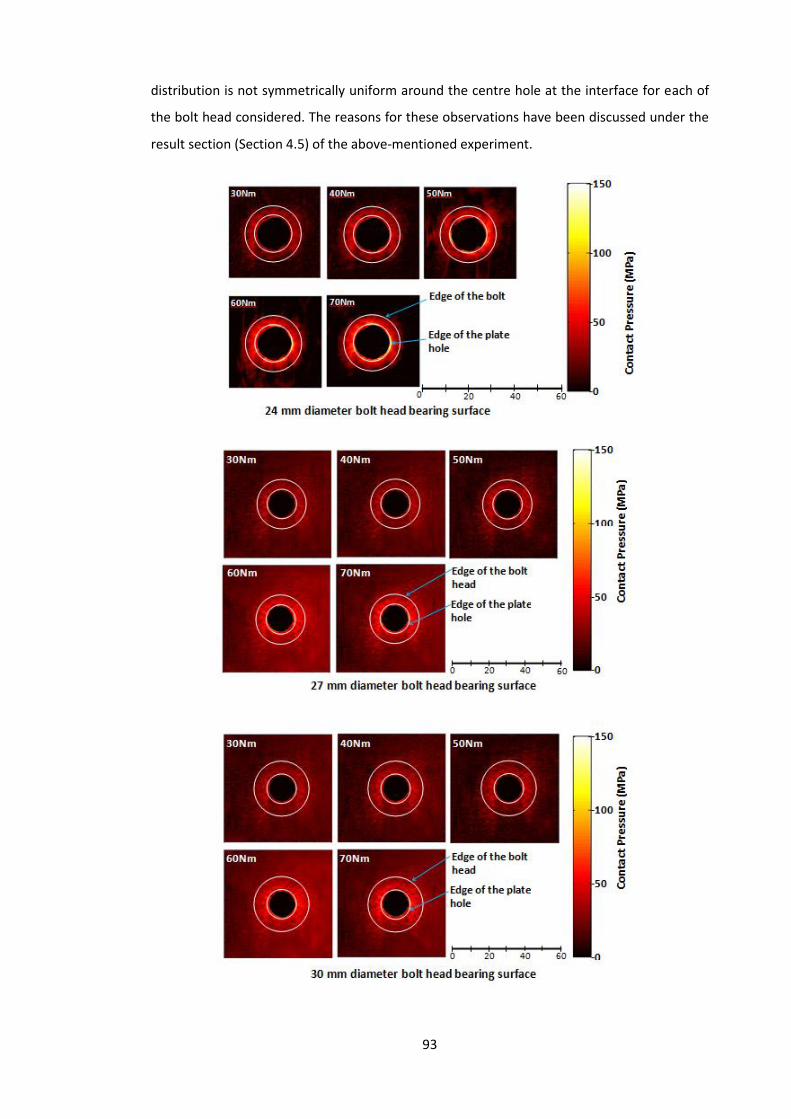
93

distribution is not symmetrically uniform around the centre hole at the interface for each of

the bolt head considered. The reasons for these observations have been discussed under the

result section (Section 4.5) of the above-mentioned experiment.

94

Figure 4.17: Contact pressure maps of bolted joints at different torques.

95

In addition to the above-mentioned features, the intensity of the bright circular zone

around the dark centre hole of the bolt is observed to reduce as the diameter of the bearing

surface of the bolt head increases. This is likely to be as a result of the pressure distribution

spreading out more, and thereby reducing the peak intensity of the contact pressure at the

interface as the bearing surface diameter increases.

Furthermore, it can be noted that the pressure spikes observed in the experimental

results under variation of plate thickness were reduced. This was due to an additional phase

introduced to processing of the experimental data. During the scanning of the bolted joints,

ultrasonic reflection was not expected from the blind tapped hole as ultrasonic pulse was not

focused in this region. Therefore, the reflected signal received from this region was likely due

to scattering from the rough surface of the blind tapped hole, and the value of this was

observed to be very small when compared with reflections from the focused regions. In

order to reduce the effect of this scattering noise, the reflected pulses at the centre of the

bolt hole (unfocused region) were averaged and any value of reflected signal that was less or

equal to this averaged value was then removed from both the reference and reflected signals

before the reflection coefficient was calculated. Though this produced a better visual of the

contact pressure maps of the bolted joints, but it has no effect on the magnitude of contact

pressure distribution as it could be noted in the result graphs (Figures 4.12 and 4.18) from the

bolt head with 24 mm bearing surface diameter.

4.10 Analysis of Bolted Joint with Varying Bolt Head

4.10.1 Average pressure line of bolted joint of varying torque and

bolt head diameter

The graphs of the calculated average contact pressure distributions are shown Figure 4.18

for the different applied bolt torques and bearing surface diameters. The figure shows results

at distances equal to and greater than the diameter of edge of the clearance hole from the

centre of the bolt hole (i.e., distance equal and greater than 8 mm from the centre of the bolt

hole). The average contact pressure distributions are average circumferential contact

pressure at different radii from the centre of the hole for each scanned contact surface as

explained in the previous analysis under bolted joints of varying plate thicknesses. This

eliminates the asymmetrical effects due to the thread, and plate profile irregularities.

96

Figure 4.18: Average contact pressure line scans of all diameters of bearing surface of

the bolt head.

From the figure, it can be seen that the peak of average contact pressure increases as the

applied load increases for each of the diameters of bearing surface of the bolt head.

However, for different diameter of the bearing surface of the bolt head, the peak of average

contact pressure distribution decreases as the diameter of bearing surface of the bolt head

increases from 24 mm to 36 mm. The peak of average contact pressure distribution decreases

from 62 MPa to 24 MPa as the diameter of bearing surface of the bolt head increases from 24

97

mm to 36 mm for the 70 Nm torque. Furthermore, it can be observed that the distance at

which the value of the average contact pressure distribution at the bolted interface tends to a

uniform value increases as the diameter of bearing surface of the bolt head increases.

These observations indicate that the pressure distribution spread out more thereby

reducing the peak intensity of the contact pressure at the interface as bearing surface of the

bolt head increases as also rightly observed in the result section above (section 4.9). These

observations were in agreement with earlier research work made by Marshall et al. [44]

where they observed that washers affect the interface pressure distribution of bolted joint

when inserted under the bolt head. The plain washer inserted under the bolt increases the

bearing surface of the bolt head, thus reducing the intensity of contact pressure at the

interface while at the same time increases the average contact pressure at the background

within the distribution. The plain washer produced a similar effect to what is observed in this

present study.

As shown in the Figure 4.18, the average contact pressure profile for each of the bearing

surfaces of the bolt head shows different degrees of smoothness. This observation is due to

the different degrees of profile irregularities of the bearing surface of the bolt heads. Figure

4.19 shows the profile graphs of 24 mm, 32 mm and 36 mm diameter surface bearing, taken

at equal 1 mm distance from the shank of the bolts. The values of 0.9 m and 5.2 m were

respectively recorded as Ra (average roughness) and Ry (maximum peak-to-valley height)

values for the standard forged M16 bolt having 24 mm diameter bearing surface, while 4.5

m and 5.7 m were recorded as values Ra, and 30.3 m and 51.7 m as Ry values for bolts

with 32 mm and 36 mm diameter surface bearing respectively. These values of profile

roughness along with the graphs show that the roughness of the bearing surface of bolt head

have a corresponding effect on the contact pressure at the bolted interface.

Figure 4.19: Surface profile of the bearing surface of the bolt heads with 24 mm, 32 mm

and 36 mm diameter.

98

4.11 Discussions on Static Scanning of Bolted Joints with

Varying Bolt Head Diameter

4.11.1 Joint loads

The total joint loads for the average contact pressure distribution for each of the torques

for ultrasonic measurement were obtained by integrating the area under curves using a

Trapezoidal method as explained under section 4.7.1. The theoretical load was also

calculated using the proposed empirical relation by Shigley and Mischike [13].

Table 4.2 shows the total joint load for the average contact pressure distribution at

various torques for all the bolt heads. From the table, it can be observed that the joint load

varies with the applied torque for all the junctions and also varies across all the junctions for

each of the torques. The difference between the minimum and maximum loads for each of

the junctions is fairly similar. The values of the joint load for the measured average contact

pressure distributions for 40, 50 and 60 Nm torques are fairly close, and at low torque of 30

Nm the values are higher and the percentage differences are equally higher when compared

to that from other applied torques. This is likely to be as a result of earlier reason (as

explained in section 4.7.1) which is the effects of surface roughness that is more pronounced

at the low load. Overall, the percentage difference between the sum of joint load of

measured contact pressure distributions and the sum of the theoretical loads are very low.

Values of 1.3, 0.2, 0.0, 0.3, 1.1 and 0.5 percent of normalised difference are calculated for 24,

27, 30, 32, 34 and 36 mm diameters of bearing surface of the bolt head respectively when

compared to the total calculated theoretical load.

99

Table 4.2: Total joint load for the average contact pressure at various torques for all the bolt heads

Total load at the junctions (kN) Percentage difference (%)

Torque (Nm)

24 mm Dia.

27 mm Dia.

30 mm Dia.

32 mm Dia.

34 mm Dia.

36 mm Dia.

Theoretical Load

24 mm Dia.

27 mm Dia.

30 mm Dia.

32 mm Dia.

34 mm Dia.

36 mm Dia.

0 10.9 10.6 10.6 10.8 10.9 9.2 9.4 16.7 12.7 12.8 15.4 15.7 5.2

40 13.6 13.0 12.3 13.2 12.3 12.5 12.5 8.5 3.8 1.6 5.3 1.3 1.5

50 17.0 14.5 15.0 14.5 14.7 15.1 15.6 8.9 7.1 4.0 7.1 6.1 1.0

60 17.8 18.4 18.5 19.0 18.8 19.0 18.8 4.8 2.1 1.5 1.2 0.0 1.0

70 19.7 21.8 21.7 20.8 20.6 21.5 21.9 9.9 0.6 0.8 4.9 6.1 1.9

Sum/avg. 79.1 77.2 78.1 78.4 77.2 78.5 78.1 1.3 0.2 0.0 0.3 1.1 0.5

Avg. = A normalized average of the percentage difference.

100

4.11.2 Mean normalised average contact pressure distribution

Figure 4.20 shows normalised average contact pressure distributions for all the torques for

all the six bolt heads. The normalised average contact pressure distributions were obtained

as explained in the section 4.7.2. The distance under the contact pressure distributions was

also normalised by dividing it the bolt radius (a).

It can be observed from the figure (Figure 4.20) that for each of the bolt heads the contact

pressure distribution profiles become approximately constant at a point irrespective of the

applied load. This observation has been explained in section 4.7.2 which is established that

the interface contact pressure only grows in intensity has applied load increases without

corresponding growth in the overall size of the pressure distribution. The distance at which

the normalised average contact pressure distributions become constant also increases as the

bolt head increases, and in the majority of the cases (except in 24 diameter bolt heads) falls

between 3 and 4 of the radius of the bolt from the edge of the bolt hole.

Furthermore, Figure 4.21 shows the variation in the means normalised average contact

pressure distributions of all the bolt head diameters. The means normalised average contact

pressure distributions were calculated from the normalised average contact pressure

distributions for each of the bolt head bearing diameter. The variation shown in the figure

implies that the contact pressure distribution at the interface of bolted joint depends on the

bolt head bearing diameter. The rate at which the contact pressure deteriorates is more

pronounced between 24 mm and 27 mm bolt heads, but this change in rate decreases as the

bolt head increases from 27 to 36 mm. This also supports the earlier observations (Section

4.10.1) that the increase in the bearing surface of the bolt head affects the interface pressure

distribution of bolted joints.

101

Figure 4.20: Normalised average contact pressure for bolt heads with varying

bearing diameter.

102

Figure 4.21: Mean normalised average contact pressure of bearing diameter of the bolt

heads.

The results of the scanning of the bolted joints show the effect the bolt geometry on the

contact pressure. The effect of non-uniform clamping from the bolt head as a result of the

helix profile of the bolt thread responsible for the non-symmetrical and non-uniformity of the

contact pressure distribution around the centre hole at the bolted interface.

From the results of the scanning of bolted joints, it is evident that the edge of the plate

hole and the bolt head significantly affect the profile of the contact pressure distribution at

the bolted interface as both acts as a stress raiser at the contact interface. A countersunk

edge of the clearance hole of the bolted plate is found to be responsible for the outward shift

in the position of the peak value of the pressure profile at the interface, and also accounts for

a steeper gradient the curves around the peak value of the pressure profile. Consequently,

this led to a higher percentage of the joint load being supported by a smaller area. This is a

clear reason for the observations noted in some research studies on bolted joints that

clearance of bolt hole has an effect on the stiffness of the bolted joints. Experimental studies

by Lawlor et al. [158] as well as analytical by Fan and Qiu [159] and also numerical studies by

McCarthy and McCarthy [160] respectively noted that an increase in clearance of the bolt

hole reduces the stiffness of bolted joints, while the ultimate strain in the joints increases.

The stiffness of a bolted joint is a combination of the stiffnesses of the bolt and the

clamped members. The accurate calculation of member stiffnesses of bolted joint is essential

103

for the determination of the preload and the resultant force in the bolt and members when

external load is applied to the joint. Since stiffness of the joint members is a function of the

contact pressure distribution at the interface, what they observed was as a result of changes

in the pressure distribution due to bolt hole clearance effect and this was similar to what is

observed in the present study. Thus, this study clearly shows the influence of the edge of the

bolt hole on the contact pressure distribution, and caution must be taken during the design

and manufacturing of bolted components not to introduce chamfer on the edge of the bole

hole during deburring.

Similar to what was observed by Marshall et al. [44] and Ziada and Abd El Latif [39], the

stress concentration effect from the edge of the bolt head influences the position of the

maximum contact pressure at the interface. The edge of the bolt head is a point of

discontinuity and acts as a stress raiser, and this increased the observed measured stress on

the interface. This stress concentration effect from the edge of the bolt head was noted to

decrease as the thickness of the bolted plate increase. Furthermore, the surface profile of

the bearing surface of the bolt head affects the contact pressure distribution at the interface.

This is because the peaks of the large asperities of the profile ridges on the surface of the bolt

head also acts as a stress concentration and consequently increased the stress at the

corresponding points on the bolted interface. Therefore, the rougher the bearing surface of

the bolt head the lesser the smoothness of the contact pressure distribution profile produced

at the interface. This result also shows that attention must be paid to the roughness of the

bearing surface of the bolt head during production of bolt so as not to introduce stress

concentrations at points on the interface of the bolted joint through rough bearing surface.

Finally, the results of ultrasonic scanning of bolted joints in this study show that the bolt

thread geometry, plate thickness, axial loads, edge of the bolt hole, edge of the bolt head,

surface profile of the bolt head and bearing surface diameter of the bolt head have effects on

the contact pressure distribution of bolted joints. The data obtained in this chapter will be

utilised in the next chapter of this thesis to model the contact pressure distribution of bolted

joints. Furthermore, the results obtained will also be explored to study bolted joints under

dynamic loads.

4.12 Conclusions

A non-intrusive method has been used to determine interface pressure in bolted

joints. This method uses reflected ultrasonic signal measurement to determine the

104

contact pressure between the bolted joint under different loads. Reflected ultrasonic

signals between samples with different upper plate thicknesses with fixed lower plate

thickness were measured to investigate the effect of plate thickness on the interfacial

contact pressure in the bolted joints. This method was also used to study the contact

pressure at the interface of bolted joint when the diameter of the bolt head varied.

It was observed from the experimental results that the edge of the bolt head played a

prominent role in the position of the peak value in the contact pressure distribution

at the interface, and the spread of the contact pressure distribution at the interface.

The experimental results show that the edge of the bolt hole has significant effects

on the profile of the contact pressure distribution at the bolted interface. The edge

of the bolt hole affects the rate at which the contact pressure decay at points very

close to the peak of the pressure distribution. The larger the edge of the bolt hole,

the higher the percentage of the joint load that would be supported by a small area

at the contact interface.

While it was observed that the contact pressure at the interface increases as the

applied load increases in all the plate thicknesses and also in all the bolt head

diameters, the distance from the edge of bolt hole at which the value of the

distribution becomes fairly constant is independent of the applied load in the plate

thicknesses and bolt head diameter.

Furthermore, the contact pressure distribution was observed to vary with the plate

thickness. The variation in the peak value of contact pressure distribution in bolted

joints was found not to depend on the plate thickness. However, the distance at

which the distribution becomes fairly constant was found to increase as the plate

thickness increases.

The experimental results show that while the peak value of the contact pressure

distribution decreases as the bolt head increases, the distance from the edge of bolt

hole at which the value of the distribution becomes constant increases as the bolt

head increases.

The distance at which the normalised average contact pressure distributions become

fairly constant also increases as the bolt head increases, and in the majority of the

cases falls between 3 and 4 of the bolt’s radius from the edge of the bolt hole.

105

Chapter 5 Weibull Modelling of Contact Pressure Distribution of Bolted Joints

Weibull Modelling of Contact Pressure Distribution of Bolted Joints

5. As a result of the advantages associated with bolted joints, numerical and

analytical models have been developed by authors to predict pressure distribution

of bolted joints. This chapter analyses the contact pressure distribution in bolted

joints. The experimental data from bolted joints with varying plate thickness and

bolted joints with varying diameter of bearing surface of the bolt head from the

Chapter four were used. A statistical model based on Weibull distribution was used

to fit the experimental data and a good correlation was observed between the

experimental and the theoretical values. Parameter (was introduced to the Weibull

distribution to adjust the amplitude of the contact pressure distribution curve from

the model to that of the experimental contact pressure distribution. The values of

both the shape and scale parameters of the Weibull distribution reflect the

experimental observations of the contact pressure distribution. Based on results

and observations, a model has been proposed to fit experimental data and this will

be of benefits to the design of bolted joints.

5.1 Introduction

Bolted joints constitute an important component used in machines and structures no

matter the degree of complexity. They are often used in large number in some of the

engineering structures such as in aircraft and rail joints. The stiffness and clamping

performance of bolted joint depends on the quantitative representation of the contact

pressure at the interface during design. As mentioned under the literature review in Chapter

2 and which will be briefly stated as a recap in this section, many research literatures have

presented numerical and analytical models to describe contact pressure distribution in bolted

joints. Some have compared their results with results from experimental tests and

reasonable agreements have been obtained. However, a limited number of authors have

attempted to fit the results of the data from experimental tests to appropriate models.

106

Mittelbach et al. [45] compared the experimental results with theoretical contact pressure

distribution models from Fernlund and Chandrashekhara. It was noted that while

Chandrashekhara model presents higher peak pressure, the contact radius presented by

Ferlund model is larger than Chandrashekhara model. They concluded that the models

presented by Fernlund and Chandrashekhara were the best to fit the experimental results.

However, Mantelli et al. [46] highlighted the Weibull distribution as an appropriate

distribution to fit to experimental data. But, as detailed in the published study, it was not

possible to explore the relationship between Weibull and bolted joint parameters in this

study. Notwithstanding, a good correlation was achieved between the fits of the

experimentally measured data and the predicted contact pressure. Their results showed that

the Weibull distribution fit the experimental data better than models from Fernlund and

Madhusudana et al.

In all research works mentioned above, the authors have presented, as appropriate,

models fit to experimental data of experiments obtained by placing pressure sensitive films

between the loaded contacting surfaces of bolted joints. But, there are issues with the

results from a modified bolted interface which can also affect the results of the models fits to

such an experimental data. Hence, there is a need to use an appropriate model to fit the

experimental contact pressure distribution data from non-intrusive experimental techniques.

The present work intends to fit a model based on Weibull distribution to bolted joint

experimental data (data obtained from non-modified bolted interface using non-intrusive

ultrasonic technique in Chapter four), and also investigate the relationship between the

parameters of Weibull distribution and that of the contact pressure distribution of bolted

joints. The intended results will not only be additional information to the body of knowledge

but also provide a method for the evaluation of contact pressure distribution in bolted joints,

and this will be beneficial to the design of bolted joints in general.

5.2 Weibull Distribution Model

The Weibull distribution is a versatile and widely used continuous probability distribution

in many fields for lifetime data and survival analysis, especially in engineering for reliability

and maintainability analysis [161]. It can be used to model a variety of life behaviours such as

human mortality, agricultural production, weather forecasting, failure of engineering

structures and components, etc.

The general three parameters Weibull density function is given by:

107

𝑓(𝑥) =𝛽

𝜂(

𝑥−𝛾

𝜂)

𝛽−1𝑒

−(𝑥−𝛾

𝜂)

𝛽

5.1

where f(x) ≥0, x ≥0 or , β > 0, η > 0, - < > +

where β is the shape parameter which established the curve shape the distribution, η is the

scale parameter, is the location parameter and x is the predictor of the parameter under

observation. The distribution can be a two parameters distribution if the value of ϒ is set to

zero. A single parameter Weibull distribution occurs when β is the only unknown parameter,

and η are set to zero and one respectively.

Weibull represents a continuous parametric distribution, and may be skewed depending

on whether there is an increasing, constant or decreasing rate of the response variable. This

particular form makes it convenient for modelling the average interface pressure distribution

in a bolted joint. The contact pressure at the interface of the bolted joint decreases from a

peak value under the bolt head, and very close to the bolt hole, to approximately zero at a

distance away from the bolt head where contact is minimal or surfaces are separated (i.e.

failure of the contract). The contact pressure distribution of the bolted joint is positively (or

right) skewed which will make the Weibull distribution a preferred choice to fit (model) the

data sets.

Since contact pressure distribution from the edge of the bolt hole to a point where there

is separation of contact surfaces is of interest, a Weibull distribution of two parameters was

applied to model the pressure distribution. The value of the location parameter, ϒ, was

obviously 8 mm in all cases; it was therefore taken as a constant. In order to fit the Weibull

distribution to the contact pressure data, a parameter was introduced. This is used to

adjust the peak of the distribution curve to that of the experimental pressure distribution in

relation to the applied load. Therefore, introducing this new parameter into the three

parameters Weibull probability distribution in equation 5.1 gives:

𝑓(𝑥) = 𝑘𝛽

𝜂(

𝑟1−𝑟0

𝜂)

𝛽−1𝑒

−(𝑟1−𝑟0

𝜂)

𝛽

5.2

where r0 (the location parameter) is the radii distance from the centre of the bolt hole to

edge of the bolt hole and r1 is the radii distance along the plate interface from the centre of

the bolt hole.

Since the location parameter is obviously constant, therefore, the applied model equation

based on the two parameters Weibull probability distribution is given as:

108

𝑓(𝑥) = 𝑘 (𝑟

𝜂)

𝛽−1𝑒

−(𝑟

𝜂)

𝛽

5.3

, β and η are the three parameters that will be investigated in order to model the contact

pressure of the bolted joint successfully.

5.3 Weibull Fitting of Contact Pressure Distribution of Bolted

Joint with Varying Plate Thickness

A Matlab loaded curve fitting tool was used to fit this Weibull distribution equation to the

contact pressure data. A non-linear least squares regression technique was applied to the

contact pressure data to estimate the β and 𝜂 parameters with 95% confidence bounds. The

optimum values of , β and 𝜂 for the contact pressure distribution of each applied torque of

the plates were obtained. As shown in Figure 5.1, the values of applied to each of the

applied torques for all of the plate thicknesses are approximately the same, and the same

value range of were used for all plate thicknesses. The average value of applied to the

distribution curve is presented in Table 5.1, and this is observed to vary linearly with the

applied load. This linear trend of can be represented by

𝑘 = 2.2𝑇 + 98 5.4

where T is the applied torque in Nm.

Figure 5.1: Plot of shape parameters against torque for the 5, 10 and 20 mm plates.

109

Table 5.1: Estimated values of , shape and scale parameters with the calculated R2 and root mean square error (RMSE) at various

torques for all the plate thicknesses

Torque

(Nm)

β Parameter η Parameter R2 RMSE

5 mm 10 mm 20 mm 5 mm 10 mm 20 mm 5 mm 10 mm 20 mm 5 mm 10 mm 20 mm

30 164 1.29 1.17 1.06 0.314 0.224 0.206 0.957 0.983 0.985 3.96 1.47 1.52

40 185 1.27 1.16 1.05 0.366 0.242 0.228 0.956 0.984 0.990 4.80 1.73 1.90

50 208 1.26 1.13 1.03 0.365 0.248 0.246 0.954 0.989 0.987 5.32 1.47 3.45

60 233 1.26 1.12 1.02 0.363 0.258 0.258 0.957 0.989 0.986 6.45 1.72 2.78

70 250 1.24 1.11 1.02 0.389 0.271 0.259 0.954 0.989 0.990 6.75 1.98 2.79

Average 1.27 1.14 1.03 0.359 0.249 0.239 0.956 0.987 0.987 4.75 1.67 2.24

110

Figure 5.2: Weibull distribution curve fits to average contact pressure line scans of 5, 10

and 20 mm plates.

111

The values of the Weibull fits (Figure 5.2) tend to a constant value at a distance of 9 mm,

13 mm and 14 mm from the bolt hole which is different by 4, 4 and 3 mm for the 5, 10 and

20 mm plates respectively when compared to the experimental data. When making this

comparison, it should also be noted that the Weibull data when tending to a limit does also

not have the inherent variation of the experimental results, due to the absence of surface

roughness effects in the model. It can also be observed that the peak amplitude of the

Weibull distribution curves fits well to experimental data for the 5 mm plate thickness, with

the accuracy decreasing as the plate thickness increases. The peak values are a little higher

in the Weibull fits than in the experimental case for the 10 mm plate, and a little lower in the

case the of the 20 mm plate. Variations in the average pressure profiles for the Weibull fits

with respect to joint geometry, as have been previously discussed in the ultrasonic results in

Section 4.7, can also be observed.

The value of shape parameter (β) obtained for each of the plates shows a near constant

trend as the applied torque increases (Table 5.1 and Figure 5.3), with average values of 1.27,

1.14 and 1.03 are recorded for 5, 10 and 20 mm plate thickness respectively, and shows a

decrease as the plate thickness increases. The small variation in shape parameter (a very

slow dropping in value as the applied torque increases, as observed in the figure), for a given

plate thickness, are in keeping with the observation in the results section that the contact

pressure distribution does not spread with an increase in applied torque, and instead

additional load is supported by a highly clamped area of the contact zone. This is also in

agreement with the assertion made by Mantelli et al. [46] that the value of β is almost

constant for a particular junction with plates of the same materials.

Figure 5.3: Plot of shape parameters against torque for the 5, 10 and 20 mm plates.

112

The value of scale parameter (Table 5.1 and Figure 5.4) increases with applied torque for

each of the plate junctions, and the same trend is also observed for all the plate thicknesses.

However, it decreases as the plate thickness increases, but with the difference in values very

small between 10 and 20 mm upper plate thicknesses.

Figure 5.4: Plot of scale parameters against torque for the 5, 10 and 20 mm plates.

5.4 Joint Loads for the Weibull Fit of Bolted Joint with

Varying Plate Thickness

The total joint loads for the Weibull fit was calculated for each of the torques

investigated. Table 5.2 shows the total joint load for the Weibull fit distributions, and also

their percentage difference to theoretical joint load at various applied torques. Integration

was performed on the results of fits in Figure 5.2 for the average contact pressure using

Simpson’s methods to get the total joint loads. The theoretical load was also calculated using

the empirical relation proposed by Shigley and Mischike [27] as stated in section 4.7.1.

113

Table 5.2: Total joint load for the Weibull fit to the average contact pressure at various

torques for all plate thicknesses

Total load at the junctions (kN) Percentage difference (%)

Torque (Nm)

5 mm plate

10 mm plate

20 mm plate

Theoretical Load

5 mm plate

10 mm plate

20 mm plate

30 12.2 12.2 12.3 9.4 30.0 30.6 30.9

40 13.8 13.8 13.9 12.5 10.6 10.7 8.5

50 15.3 15.4 15.5 15.6 2.0 1.5 1.3

60 17.8 17.3 17.3 18.8 5.3 7.9 7.6

70 18.7 18.8 18.8 21.9 14.6 14.1 13.9

Sum/Avg. 77.8 77.5 77.8 78.1 0.5 0.8 0.4

Avg. = A normalized average of the percentage difference.

Table 5.3: Comparison of total joint load for the measured and the Weibull fit at various torque for all plate thicknesses.

Torque (Nm)

Load at the 5 mm plate Junction (kN)

Load at the 10 mm plate Junction (kN)

Load at 20 mm plate Junction (kN)

Experiment Fit Experiment Fit Experiment Fit

30 12.8 14.1 13.5 12.6 13.1 12.8

40 14.6 16.0 13.6 14.7 10.9 12.9

50 16.4 17.6 11.2 16.3 16.7 16.8

60 18.8 19.4 22.5 18.6 17.3 19.0

70 19.8 20.9 19.9 20.0 24.1 20.6

Sum 82.4 88.1 80.7 82.2 82.0 82.1

As shown from the table (Table 5.2), overall correlation is good between the theoretical

load and the Weibull fit. The maximum deviation with respect to theoretical values occurs at

the lower end of applied loads, and is likely due to the accuracy of the torque wrench used to

tighten the bolt. However, overall due to the main aim of the section is to study and model

the effects on the pressure distribution of plate thickness, this result is acceptable.

Furthermore, the good correlation between the theoretical joint loads and the predicted

values from the model (Table 5.3), also indicate the appropriateness of the modelling

approach followed.

114

5.5 Weibull Fitting of Contact Pressure Distribution of Bolted

Joint with Varying Bolt Head Diameter

A non-linear least squares regression technique was applied to the contact pressure data

of bolted joint with varying bolt head to estimate the β and 𝜂 parameters with 95%

confidence bounds. The optimum values of , β and 𝜂 for the contact pressure distribution

of each applied torque of the bolt heads studied were also obtained. The Weibull fits are

presented in Figure 5.4 while the values of the Weibull fits parameters are presented in Table

5.3. Unlike in the case of variation in plate thickness of bolted joint where approximately the

same values of were applied to each of the applied torque, the values of applied to each

of the torques for all the bolt heads are not same, therefore different values of were used

for all bolt heads. As presented in Table 5.5, the values of applied to the distribution curve

for each of the bolt heads are observed to vary linearly with the applied load and at the same

time varied from one bolt head to another.

From the Weibull fits (Figure 5.5), it can be observed that the peak amplitude of the

Weibull distribution curves fits well to that of the experimental data. The values of the

distribution curve (Weibull fits) tend to a constant value at approximately distance of 13 mm,

20 mm, 21 mm, 21 mm, 23 mm and 24 mm from the bolt hole which is different by 4, 6, 7, 6,

9 and 9 mm for the 24, 27, 30, 32, 34 and 36 mm bolt heads respectively when compared to

the experimental data. As earlier said in section 5.3, the variation between the Weibull and

experimental profile convergence to a limit is due to the absence of surface roughness in the

model. This can also be said to responsible for the increase in differences between Weibull

fits data and experimental data at the point where they tend to a constant value as the

diameter of the bearing surface of the bolt head increases.

115

Figure 5.5: Weibull distribution curve fits to average contact pressure line scans for all

the bolt heads.

116

Table 5.4: Estimated values of, shape and scale parameters at various torques for all the bolt heads

Torque

(Nm)

β Parameter η Parameter

24 mm 27 mm 30 mm 32 mm 34 mm 36 mm 24 mm 27 mm 30 mm 32 mm 34 mm 36 mm

30 114 1.17 1.10 1.21 1.06 1.08 1.17 0.224 0.234 0.161 0.230 0.179 0.138

40 138 1.16 1.09 1.16 1.09 1.09 1.13 0.242 0.211 0.188 0.188 0.176 0.121

50 168 1.13 1.11 1.19 1.10 1.06 1.11 0.248 0.196 0.166 0.191 0.176 0.133

60 193 1.12 1.08 1.09 1.08 1.05 1.15 0.258 0.199 0.188 0.182 0.173 0.130

70 225 1.11 1.06 1.10 1.10 1.08 1.17 0.271 0.187 0.180 0.171 0.157 0.115

Average 1.14 1.09 1.15 1.09 1.07 1.15 0.249 0.205 0.176 0.192 0.172 0.127

Table 5.5: Calculated R2 and root mean square error (RMSE) for the estimated shape and scale parameters at various torques

for all the bolt heads

Torque (Nm)

R2 RMSE

24 mm 27 mm 30 mm 32 mm 34 mm 36 mm 24 mm 27 mm 30 mm 32 mm 34 mm 36 mm

30 0.983 0.988 0.995 0.994 0.993 0.960 1.47 0.67 0.39 0.48 0.41 0.67

40 0.984 0.988 0.992 0.991 0.995 0.980 1.73 0.82 0.60 0.64 0.42 0.62

50 0.989 0.993 0.990 0.992 0.995 0.987 1.47 0.75 0.77 0.72 0.54 0.67

60 0.989 0.991 0.995 0.993 0.996 0.987 1.72 0.95 0.69 0.72 0.55 0.72

70 0.989 0.990 0.993 0.993 0.993 0.988 1.98 1.08 0.86 0.81 0.77 0.83

Average 0.987 0.990 0.993 0.993 0.994 0.980 1.67 0.85 0.66 0.67 0.54 0.70

117

Table 5.6: Applied values of at various torques for all the bolt heads

Torque (Nm)

24 mm 27 mm 30 mm 32 mm 34 mm 36 mm Average

30 164 108 112 105 102 90 114

40 185 142 128 135 116 116 137

50 208 180 155 155 147 142 165

60 233 208 182 180 178 168 192

70 250 248 220 210 208 202 223

Different values of are applied to each of the torques to fit the model to the

experimental data for all the bolt heads (shown in Table 5.6 and Figure 5.6). This shows that

the diameter of the bolt head affect this parameter which is used to adjust the peak of the

distribution curve to that of the experimental pressure distribution in relation to the applied

load. However, for each of the bolt head diameter it is observed that the applied to vary

linearly with the applied load. This variation in value of as the bolt head increases, as

noted in Figure 5.6, is due to the fact that the peaks of contact pressure at the interface are

affected by the area of contact between the bolt head and the bolted plate as noted in the

work of Marshall et al. [44], and explained in section 4.11 of this thesis work. The variation of

to the bolt head diameter could be represented by the linear trend equation:

𝑘 = −4.6𝑑 + 306 5.5

where d is the diameter of the bolt head.

Figure 5.6: Plot of applied against torque for all the bolt heads.

118

Figure 5.7: Plot of applied against torque for all the bolt heads.

Figure 5.8: Plot of shape parameter against torque for all the bolt heads.

As shown in Table 5.4 and Figure 5.8, the value of the shape parameter (β) obtained for

each of the bolt heads does not show a linear trend as the diameter of the bolt head

increases, but the trend varies almost the same way for all the applied loads. Unlike the value

of the shape parameter for the joints with varying plate thickness where standard forged

M16 bolts with 24 mm diameter bearing surface with similar surface profiles were used, the

in-house manufactured bolts for the remaining diameters of the bearing surface have varying

surface profiles, especially at the edge of the bolt head. As shown in Figure 5.9, bolts with 30

mm and 36 mm bearing surface show a surface profile that decreases from a distance from

119

the edge without a fairly sharp edge observed in the 24 mm diameter bolt head bearing

surface. Their values increase than normal, and did not follow the expected trend as

observed in the shape parameter for the joints with varying plate thickness. Except for 27

mm bearing surface, the remaining profiles are close to the 24 mm diameter bearing surface

bolt head and their values follow a trend seen in joints with varying plate thickness. The 27

mm diameter bolt head bearing surface has a very sharper edge than the 24 mm diameter

bolt head bearing surface and that is responsible for its value decreasing so much. This effect

of the edge of the bolt profile is very pronounced at low loads, but decreases as deformation

of the bearing surface at the edge of the bolt head increases at the high loads.

Figure 5.9: Surface profile of the edge of the bolt heads with 24 mm, 32 mm and 36

mm diameter of the bearing surface.

In Figure 5.8, the average values of 1.14, 1.09, 1.15, 1.09, 1.07 and 1.15 are recorded for

24, 27, 30, 32, 34 and 36 mm bolt heads respectively, which shows that the trend varies

between 1.15 and 1.07 as the bolt head diameter increases. Furthermore, it can also be

observed that a small variation of less than 0.07 is recorded in the shape parameter for most

cases for all loads for a given bolt head. This is due to observations explained in Section 4.5

that the contact pressure distribution does not spread with an increase in applied torque.

From Table 5.4 and Figure 5.10, it can be observed that the value of scale parameter

decreases as the bolt head diameter increases, and the same trend is also observed for

almost all the applied loads. The average values of 0.249, 0.205, 0.176, 0.192, 0.172 and

0.127 are recorded for 24, 27, 30, 32, 34 and 36 mm diameter bolt heads respectively. These

values are affected by the unsteady values recorded at low torque of 30 Nm when the effect

of surface roughness is more pronounced. Overall, a decrease in trend is observed.

120

Figure 5.10: Plot of scale parameter against torque for all the bolt heads.

5.6 Joint Loads for the Weibull Fit of Bolted Joint with Varying

Diameter of Bolt Head

The total joint loads for the Weibull fit to the average contact pressure of bolted joint of

all the applied torques for the bolt head diameters considered and the theoretical loads were

calculated as outlined in Section 5.4 and presented in Table 5.7. As shown in the table,

maximum deviation with respect to theoretical values occurs at the lower end of applied

loads. As stated earlier in Section 5.4, this deviation is likely due to the accuracy of the

torque wrench used to tighten the bolt and also the inherent effect of the surface roughness

on the experimental data used for the Weibull fits. Furthermore, there exists an acceptable

low percentage difference between theoretical joint loads and the predicted values from the

Weibull fits. Therefore, going by the main aim of this section which is to study and model the

effects Bolt head diameter on the contact pressure distribution, this indicates that Weibull

distribution modelling can model the contact pressure diction of a bolted jointed.

121

Table 5.7: Total joint load for the Weibull fit to the average contact pressure at various torques for all the bolt heads

Torque

(Nm)

Total load at the junctions (kN) Percentage difference (%)

24 mm 27 mm 30 mm 32 mm 34 mm 36 mm Theoretical

Load 24 mm 27 mm 30 mm 32 mm 34 mm 36 mm

30 12.2 9.2 10.6 10.6 10.9 9.6 9.4 30.0 2.3 12.6 12.6 16.2 2.5

40 13.8 12.0 12.1 13.6 12.4 12.9 12.5 10.6 3.7 3.5 8.6 0.9 3.3

50 15.4 15.3 14.6 15.6 15.7 15.8 15.6 2.0 2.3 6.5 0.3 0.4 1.4

60 17.3 17.6 17.2 18.1 19.0 18.9 18.8 5.3 5.9 8.5 3.5 1.3 0.6

70 18.8 21.0 20.7 21.1 22.2 22.6 21.9 14.1 3.9 5.2 3.5 1.5 3.4

Sum/Avg. 77.5 75.1 75.1 78.9 80.2 79.8 78.1 0.8 3.8 3.9 1.0 2.6 2.2

Avg. = A normalized average of the percentage difference.

122

5.7 Discussion

The results from the fitting of the Weibull distribution to the experimental contact

pressure data of bolted joints with different plate thicknesses, and also that of varying bolt

head bearing diameters, present a good indication that the contact pressure in bolted joints

can be modelled appropriately with a Weibull curve. The constant profile of the contact

pressure distribution as seeing in Figure 4.13 further validate the use of single ‘’ factor in the

modelling, which adjust the amplitude of the distribution curve to that of the experimental

pressure distribution in relation to the applied load. The parameter increases with the axial

load as expected (Table 5.1, Table 5.4 and Figure 4.16 reinforce this), since it is responsible

for the increase in the amplitude of the curve and it is approximately constant in all plate

thickness for a particular axial load. This can also be observed for any particular bolted joint

junction for the entire bolt head diameters considered.

Figure 5.11: Plot of average values of the shape and scale parameters against the plate

thickness.

The average values of the shape (β) and the scale (η) parameters show almost the same

trend when plotted against the plate thickness (Figure 5.11). Between Plates 5 and 10 mm

thick there is a sharp decrease in the value of β while the amount of variation between plate

10 and 20 mm is quite small and this can be attributed to the effect of the amount of

difference in thickness as the plate thickness increases. It can be observed in Figure 5.11 that

the average value of β is greater than one in all the plate thicknesses. This indicates that the

contact pressure deteriorates with distance from the bolt hole, and this β value decreases

with an increase in plate thickness as it characterises a reduction in the rate of deterioration

with the distance from the bolt hole (as explained earlier with Figure 4.14 in Section 4.7.2).

123

In Table 5.1 and Figure 5.11, the scale parameter decreases in value as the plate thickness

increases indicating that the peak of the contact pressure distribution gets pushed towards

the left. This change in shape factor is likely to be the result of the dominance of the stress

concentration from the edge of the bolt head, which is less pronounced as the plate thickness

increases. This leaves the effect of discontinuity at the edge of the bolt hole to influence the

distribution, resulting in the described peak moving closer to the location.

Figure 5.12: Plot of average values of the shape and scale parameters against the plate

thickness.

The result from the Weibull modelling of bolted joints with a varying bearing surface

diameter of the bolt head (Figure 5.12) shows that the scale parameter decreases in value as

the diameter of the bolt head increases which means that the peak of the contact pressure

distribution gets pushed towards the left. This is an indication of the dominance of the stress

concentration from the edge of the bolt head is also less pronounced as the bearing diameter

of the bolt head increases. As seen in the Figure 5.12, the average value of shape parameter

is greater than one in the bolt heads considered. This indicates that the contact pressure

deteriorates with distance from the bolt hole. Also, the shape parameter does not show a

definite decrease in the average value as the bolt head increases, and with the overall

decrease trend in the average value of the shape parameter as the bolt head increases,

indicates that the distribution spread out at the background at the contact interface under

the bolt head as earlier observed and explained in Section 4.11.

Furthermore, the small changes (reduction) in average values of the shape parameter in

bolted joints with varying plate thickness and bolt head as the axial load increases means a

reduction in rate of depreciation in contact pressure distribution. This can be an indication

124

that more asperities within the contact region under the bolt head come into contact and

support the increasing load.

5.8 Conclusions

A model based on Weibull distribution function was used to fit the experimental data

and a good correlation was observed between them. Hence, it implies that Weibull

distribution can successfully describe the contact pressure distribution in bolted

joints. The Weibull parameters were obtained (with 95% confidence intervals) using

a least squares fit.

It was observed that parameter (the parameter introduced to adjust the amplitude

of the contact pressure distribution curve from the model to that of the experimental

average contact distribution) linearly depends on applied load. This parameter

suitably fits the amplitude of contact pressure curves in the model to that of the

experiment contact pressure profiles.

The values of both the shape and scale parameters were observed to decrease as the

thickness of the plate increases, and this was reflective of experimental observation

of the contact pressure distribution being stretched and skewed with an increase in

plate thickness.

Between plates 5 and 10 mm thick there is a sharp decrease in the value of β while

the amount of variation between plate 10 and 20 mm is quite small and this can be

attributed to the effect of the amount of difference in thickness as the plate thickness

increases.

There was a very small non-linear change in the average value of the shape

parameter while scale parameter was observed to decrease as the bolt head

increases. This also supported the experimental observation that the contact

pressure distribution spread out at the background at the contact interface under the

bolt head as the bolt head increases.

Furthermore, the value of shape parameter shows a near constant trend as the

applied load increase and is consistent with the lack of spread experimentally

observed in the contact pressure profiles with increasing load.

125

Chapter 6 Relaxation of Clamping Pressure of Dynamic Bolted Joints

Relaxation of Clamping Pressure of Dynamic Bolted Joints

6. Bolted joints are widely used in a variety of engineering applications such as in

transportation, structures and machinery, many of which are dynamically

loaded with frequencies of vibration spread over a wide spectrum with the

same general effects. When under dynamic loading, bolted joints can become

loose due to a loss in clamping pressure in the joints. This vibrational loosening

sometimes can cause serious problems, and in some cases can lead to fatal

consequences if it remains undetected. The contact pressure distribution at the

interface of bolted joints under static loads had been characterised and

modelled in chapters four and five of this thesis. The present chapter

investigates the loosening of bolted joints due to dynamic shear loading using a

novel non-invasive ultrasonic technique, with the objective to understand

mechanisms of joint relaxation and also, to establish a method of monitoring

bolted joints subjected to dynamic loading.

6.1 Introduction

One of the major advantages of threaded fasteners over other fastening methods is that the

joint components can easily be assembled and disassembled, and also re-used (especially for

maintenance purposes). The threaded fastener can be tightened and loosened, and this

remarkable feature often creates problems if the fastener turns loose, unintentionally, in

operation. Bolted joints provide a high clamp force, and this clamping force is also known as

pre-tension or bolt preload. Bolt preload is created as soon as tightening torque is applied,

even in the absence of external tensile load, which moves the bolt head against a clamped

component. The bolt head and the thread generate the preload in the bolted joint. The more

thread mating the more the preload is generated. When a bolted joint is tightened, a pitch

difference exists on the surface between the bolt and the thread. If the thread was not

damaged by the pitch difference, the bolt is stretched and the resulting preload is a function of

this axial elongation and joint stiffness.

As mentioned in the literature review in chapter 2, when a bolt is tightened, there exists a

moment due to a stored torsion in the bolt during tightening and helical geometry of the

thread that tends to produce a loosening moment of the bolt.However, this loosening moment

is resisted by the friction force between the bolt and nut threads caused by the stretching of

126

the bolt. Therefore, the bolted components will be compressed together by the action of the

tension in the bolt and the joint would be locked by the friction of the threads. These frictional

forces between the threads surfaces must be greater than any tangential surface forces that

might act to oppose them and this is to be maintained throughout the service life of the joint in

order to prevent relative movement, wear and fretting, etc. But when bolted joint is subjected

to dynamic loads in the form of impact, vibration, cyclic thermal loading it often fails due to

either fatigue or vibration induced loosening [24]. In some cases, these failures are of fatal

consequence, and hence, they are safety critical [6-8, 15, 16].

It is a common understanding that in some circumstances a joint that is well designed to

retain sufficient prevailing (residual) load after initial non-rotational relaxation losses will

overcome the service load without loosening even in the absence of any locking device [10, 11,

26]. However, bolted joints turn loose in service, and a detailed procedure for the design of

bolted joint of this nature requires full information of all forces on the joint and, most times,

such knowledge is not available. Hence, designers commonly specify the use of a fastener

locking device on the fastener in a joint during installation to prevent loosening. Studies

conducted to assess the performance of these locking devices have shown that the majority of

them do not totally lock the fastener, but tolerate some degree of self-loosening under

dynamic shear loading [27, 28]. Therefore, it is not only important to understand the

loosening mechanism in bolted joints and existing design parameters for optimised resistance

to loosening, but monitoring of such phenomenon in service is also important especially when

their operations are of safety concern.

As earlier mentioned in the literature review, the problem of unintentional loosening of

bolted joints has been identified since it came into prominence during the industrial revolution

in the nineteenth century, especially in the rail industry [47]. While a documented investigation

into the process that led to self-loosening was first conducted in 1945 when Goodier and

Sweeney [49] studied loosening of bolted joints subjected to axial dynamic loading, a key

theory of vibrating self-loosening of bolted joints under dynamic loads was explained by

Gerhard H. Junker in his influential paper on the self-loosening of threaded fastener in 1960. He

showed that self-loosening induced by transverse vibration perpendicular to the thread axis is a

major cause of failure in bolted joint subjected to dynamic shear loading. Several research

works in this area were based upon the principle of the Junker transverse vibration test

machine, and the preload decay curve produced from his vibration test results also becomes

the assessment method for measuring loosening resistance of a fastener. Since that time, self-

loosening of the bolted joints due to transverse vibration has been the subject of many

research studies.

127

In both the analytical and numerical studies of loosening of bolted joints, assumptions were

made about the contact conditions of the interfaces (for example, while an estimated constant

value of friction coefficient is usually applied in numerical investigations, it has been shown

that the value of the friction coefficient is not always constant as tribological properties of the

mating surfaces often change as they slip during loosening [54, 162]. These assumptions are

issues in the true representation of the operating conditions when bolted joints are subjected

to vibration induced self-loosening. In most of the experimental studies, the loosening of

bolted joints was decided by the amount of pre-torque in the joint. Some of the techniques

applied include torque control methods through a calibrated wrench and extension control

using ultrasonic methods to monitor the extension of the bolt which was then calibrated to

torque. Impedance based techniques using embedded piezo-electric elements were also

employed in some studies for damage detection in structural health monitoring of bolted joints

[85, 163, 164]. One of the disadvantages of some of these techniques was that they cannot be

used to gather information during test setup. Except in the studies conducted by Marshall et

al. [76] and the use of Lamb waves by Yang and Change [165], the measurements were only

restricted to the fasteners in the techniques that can be used during test setup. They failed to

gather information from the clamped interface, which is a critical element of the bolted joint.

While in service, bolted joints are subjected to additional shear loads in other directions to the

cyclic shear load and such loads were also previously ignore.

Although, the research studies of Marshall et al. [76] presented a proof of concept the

ultrasonic reflections from the clamped interface could be used to assess the progress of

relaxation in bolted joints, these studies were limited to the measurement of the relaxation of

contact pressure at a few discrete points of the bolted plate interface. Therefore, the present

study intends to rigorously explore this technique to study the response of the bolted interface

pressure as well as the reaction of the fastener to the vibration loosening induced by

transverse shear loading. A greater number of bonded contact transducers will be employed to

continuously monitor the loosening of bolted joints subjected to varying bolt torque, cyclic

shear load, frequency and additional transverse load in order to determine the effect of these

factors on the loosening of the joints. Furthermore, change in the tension in the bolt and

rotation of the bolt head, as well as the change in the contact pressure at the clamped

interface will be monitored during the of the joints relaxation with the intention to understand

the mechanisms of bolted joint loosening, and also to establish a practical condition

monitoring technique for bolted joints.

128

6.2 Experimental Procedure

6.2.1 Test specimens

The bolted joint specimen used in this study consisted of steel plates manufactured from

EN24 steel and clamped together with an M12 (grade 8.8) steel bolt. Figure 6.1 shows a not-

to-scale diagram of the specimens. The front plate of the specimen had a clearance hole

through it while the back plate had a threaded hole through. The contact surfaces of both

plates were ground to an average surface roughness of about 0.5 m (Ra). This was to

minimise the effect of wear during dynamic shear loading of the bolted joint. Both plates had

equal thickness of 10 mm and three holes of 8 mm diameter were drilled through each plate,

so that they can be bolted to the dynamic loading rig. The contact surface area between the

plates when bolted was approximately 2947 mm2. The back plate (Plate A) was to have the

transducers mounted on the under-side of it, while a transducer will equally be attached to

top of the bolt. A 5 mm diameter hole was also drilled through the Plate B parallel to the

centre of the clearance hole. This is to allow for the introduction of additional transverse side

loads to the dynamic shear load acting on the bolted joint during the experiments.

Figure 6.1: Test specimen (plates and bolt).

129

6.2.2 Instrumentation of the specimen

This ultrasonic technique uses piezoelectric elements bonded directly to the exterior

surface (i.e. underside) of the threaded plate (Plate A) of the bolted components to generate

an ultrasonic pulse when excited by a voltage signal. This ultrasound wave propagates

through the plate to the clamped interface. The energy of the wave is partially reflected back

to the element while the remaining is lost through the contact at the asperity junctions and

also to attenuation in the material as explained in Section 3 of Chapter 3. A pulse-echo

method of piezoelectric transducer configuration was used in this study, which involves the

use of the same transducer to act as both the transmitter (sending the pulse) and receiver

(sensing the reflection) of ultrasonic signals.

The transducer used for this study was made from low cost, off the shelf piezoelectric

discs formed from high sensitivity lead zirconate titanate (PZT), and it came pre-sputtered

with wrap around electrodes of silver (this is naturally the negative terminal of the sensor).

The discs have a centre frequency of 10 MHz, a nominal diameter of 7.1 mm and thickness of

0.2 mm. The spatial resolution of the measurements depends partially on the geometry of

the sensor. Hence, in order to maximise the resolution of the transducer to provide a narrow

sensing area, the disc elements were cut down to form 2 mm 1 mm active area transducers

(Figure 6.2). When these were excited, they emitted a gradually diverging ultrasonic sound

wave approximately equal to the dimension of the sensors’ active area.

Figure 6.2: Original and modified miniaturised PZT elements.

The transducers were permanently bonded directly to the back of the plate (Plate A with

the threaded hole) with adhesive. It is important that the sensors were well bonded to the

surface of the specimen to ensure good acoustic coupling that will allow sufficient ultrasonic

energy to pass into the specimen. M-bond 610 (Vishay) adhesive was used because of its

good gluing strength and low viscosity which allow it to form a thin adhesive layer down to 5

m. When the adhesive was applied and the sensors were placed into position, pressure was

then applied to the sensors through a sprung clamp coupled to the sensors with flexible

silicone rubber. This is to provide evenly distributed loading and also to prevent transducer

130

cracking during curing. The adhesive was then cured at elevated temperature of 150 0C for 1

hour 30 minutes while the pressure on the sensors was continuously maintained.

When the adhesive finally cured, a very thin layer of the adhesive was formed between

the sensor and the specimen, due to the low viscosity of the adhesive, and as the load

applied that squeezed out the excess adhesive from the contact gap between the sensor and

the specimen during the curing process. This allowed asperity contact between the two

surfaces which implies that the lower electrode of the sensors can be electrically coupled to

the surface of the specimen.

This asperity contact that permits electrical coupling between the sensors and the

specimen was beneficial in two ways. Firstly, as explained earlier in chapter 3, the

piezoelectric sensor used in this study was a through-thickness resonant elements which

must be electrically excited through connections to the electrodes at its two sides. Since a

very evenly bonded piezoelectric sensor is important for good acoustic coupling and

transmission, this means that the side that was well glued to the specimen which is the

‘lower’ electrode of the piezoelectric sensor is not exposed for wiring and only the ‘upper’

electrode is exposed for wiring and connections. But with the configuration of the

piezoelectric sensor used in this study (as shown in Figure 3.7), the wrap-around electrode is

an extension of the ‘lower’ electrode that was glued to the specimen. This configuration

permits electrical wiring of both electrodes to be connected from the top surface of the

sensor without disrupting the bond between the sensor and specimen interface. Therefore,

if the wrap-around electrode of a sensor failed at the curved perimeter of the sensor so that

connection to the lower electrode breaks and there is another bonded sensor with a good

wrap-around electrode, the coupling of the sensors’ surfaces, electrically, to the specimen

means that the specimen will serve as an electrical path between the two sensors and thus,

the sensor with the failed electrode will be electrically excited. This was helpful as once the

sensors are glued it becomes impossible to remove one sensor without damaging the

remaining ones.

Furthermore, the coupling of the surface of the sensors through asperity contacts to the

specimen is also useful if only the upper electrode is exposed without the wrap-around

electrode, the ‘lower’ electrode that is glued to the specimen can be connected by using the

specimen as the connection terminal. This advantage was particularly utilised in the course

of this research during the instrumentation of specimen for the tests due to space constrain.

Once the sensors have been bonded to the specimen, a coaxial cable was then wired to each

transducer through a short cooper ‘winding’ wire that terminated at the sensor end. The

131

bonded sensors along with soldered wires were then covered with epoxy resin at the points

where they were soldered. This was to partly suppress transducer ‘ringing’ (i.e. back echo)

and also to provide protection for the sensors from damage during handling and experiment.

Two sets of test specimens with identical configurations were produced. The first set has

an array of 8 transducers directly bonded to the back of the threaded plate, while the second

set of the test specimens has an array of 32 transducers also directly bonded to the back of

the threaded plate.

6.2.2.1 8 transducer array

The placement of the transducers in this array was determined by the pressure map from

static scanning as shown in Figure 6.3 (a). As it can be seen and discussed earlier in Chapter 4

under static scanning of bolted joints, the pressure distribution map has peak pressures

located very close to the edge of the bolt hole and this pressure diminishes as the distance

from the edge of the bolt hole increases. Figure 6.3(b) shows the positions at which the

sensors were bonded on the specimen to obtain measurements during the dynamic bolted

joint experiments with the 8 transducer array. This particular transducer array was designed

to clearly identify the peak of contact pressure and show the difference in the clamping

pressure away from the bolt hole, with the array spread out to cover a large portion of the

pressure distribution radially. As shown in the layout (Figure 6.3 (b)), four sensors were

equally placed at a radius of 7 mm from the centre of the bolt hole. This was aligned to

coincide with the peak in the contact pressure distribution at the interface. The remaining

four transducers were placed at 1 mm intervals in a line from one of the first four placed

sensors. The sensors were bonded directly to the back of the plate with a threaded hole.

Figure 6.3 (c) shows the bonded transducers with copper ‘winding’ wire soldered to them at

the their respective terminals, while Figure 6.4 (d) shows the finish instrumented plate with

coaxial cable and epoxy cover.

132

Figure 6.3: (a) Typical map of scan of static bolted joint, (b) Layout of 8 transducer array

with identifying numbers, (c) Specimen with bonded sensors and (d) Instrumented

specimen.

6.2.2.2 32 transducer array

In order to monitor and obtain measurements at more points in areas of high clamp

pressure during the dynamic bolted joint experiments, a 32 transducer array was designed,

positioned and bonded to the back of the plate with the threaded hole, as shown in the

layout figure (Figure 6.4 (a)). As shown in a detailed layout in figures 6.4 (b), the sensors

were grouped into four groups of eight sensors each, and sensors in each group were

numbered from 1 to 8. All transducers with identical number in all the groups were

positioned equally in radial distance from the edge of the bolt hole. In all the groups, sensors

numbered 1 and 5, 3 and 7, 2 and 6, and 4 and 8 were respectively positioned at radial

distance of 7 mm, 8 mm, 9 mm and 10 mm from the centre of the bolt. The sensors were

evenly distributed around the threaded hole with each sensor separated, circumferentially,

by an angle of 22.50 from adjacent transducers (as shown in the figure). Furthermore, for

133

each of the sensors, the longer dimension was placed in the circumferential direction as this

will maximise the resolution of the sensor in the radial direction.

Figure 6.4: (a) Layout of the 32 transducer array on plate at different radius from the

centre; (b) Layout of sensors with identifying numbers and groups; (c)

Transducer array and (d) Specimen with transducers.

From the layout geometry of the 32 transducer array, the 32 sensors were designed to

occupy a small annulus area of approximately 265 mm2, and this placed a limitation on the

size of sensors that could be used. As a result of this constraint, 2 mm 1 mm sensors (as

shown in Figure 6.4 (c)) were cut from the active area of original disc sensors without the

wrap around electrode. These were bonded directly to the back of the plate with threaded

hole, with only the upper electrodes of the sensors exposed for electrical connection. Due to

the low viscosity of the adhesive and the gluing technique used, as explained earlier, there

were asperity contacts between the surfaces of the sensors and plate, and this allowed the

134

lower electrode of the sensors to be electrically coupled to the surface of the specimen.

Thus, the lower electrodes of the sensors were connected by using the specimen as an

electrical terminal. Therefore, the negative terminal of the coaxial cable was soldered directly

to the specimen. Figure 6.4 (d) shows the picture of the instrumented specimen with the

transducer array.

6.2.2.3 Instrumentation of bolt head

Each of the bolts used in the dynamic tests was instrumented in order to monitor the

relaxation of tension in the bolt during vibration. A piezoelectric sensor of dimension 7.1 mm

2 mm cut down from the larger PZT disc was centrally positioned, bonded directly to the

bolt head with M-bond 610 (Vishay) adhesive. After co-axial data wire had been soldered to

the terminals of the sensor, the sensor along with the wire at the soldered point was then

covered with epoxy resin to protect it from damage during handling. Figure 6.5 shows the

layout and photo of the sensor on the bolt, and also the instrumented bolt.

Figure 6.5: (a) Layout of the transducer on the bolt, (b) Glued sensor on the bolt

head and (c) Complete instrumented bolt.

6.2.3 Ultrasonic Equipment for Dynamic Bolted Joint Experiments

The equipment used to generate and receive ultrasonic signals for the dynamic scanning

tests consists of a PC (FMS100 System) fitted with an ultrasonic pulser-receiver (UPR),

digitiser and multiplexer cards. The PC sends controlled electrical excitations to the

piezoelectric element in the transducers through the UPR and the multiplexer, and the

transducers convert the electrical excitations to ultrasonic signals that are consequently

emitted to the targeted contact interface. A schematic diagram of the ultrasonic equipment is

shown in Figure 6.6. The reflected ultrasonic signals from the interface are received and

135

converted to electrical signals in the transducers, and then passed to the same PC through

the multiplexer. The PC displays both the emitted and reflected signals.

Figure 6.6: Schematic diagram of ultrasonic equipment.

As mentioned earlier under the ultrasonic equipment in chapter 3, the UPR system had

the capacity of running up to 8 channels at a time with one sensor connected to each

channel. Sensors were connected to the channels by push-fit SMB connectors. When

multiple sensors were running simultaneously, they were pulsed continuously in a flowing

manner from the first to the last sensor (i.e., 0, 1, 2, 3, 4, 5, 6 and 7 nonstop). Since the

resources of the pulser were shared among the connected sensors, the implication of this

was that the pulse rate decreases as the number of sensors connected increases. For

example, if the pulse rate was set to 40 kPulse/s and all the ports were connected to sensors;

each sensor would be pulsed at a rate of 5 kPulse/s.

Moreover, since the maximum number of sensors that could be connected to the UPR

system on the PC was 8, it implied that a manual ‘changeover’ would be required to

physically disconnect one set of sensors and connect another set if the number of sensors of

interest was more than 8. For the present test with 33 sensors (including the sensor on the

bolt head), it would be improper to use this manual ‘changeover’ method because the bolted

joint will be continuously and simultaneously monitored by the sensors while the test runs,

and manual disconnection of one set of 8 sensors and connection of another set would not

only mean that the test will be constantly stopped to ‘changeover’ the sensors, but could also

be prone to operator error.

The solution chosen was to utilise the multiplexer switch card installed on the PC to

sequentially distribute signals and ‘changeover’ the sensors at a predetermined speed. A

multiplexer connector with 64 ports was designed and constructed. As shown in Figure 6.7, it

has a box with 64 channels of push-fit SMB connectors through which cables from the

sensors were connected, along with a male 200-way LFH PCI connector block (purchased

136

from Pickering Interfaces Ltd.) through which the 64 push-fit SMB connectors were

connected to the computer controlled multiplexer switch card on the PC. 8 push-fit SMB

connectors were used to connect the multiplexer switch card through the 200-way LFH PCI

connector block to the UPR on the PC.

Figure 6.7: (a) the multiplexer connector and (b) the multiplexer connector in operation.

When the multiplexer was in operation during the test, the 8 channels on the PC were

continuously pulsed by the UPR, and the signals from these channels were transmitted to the

multiplexer switch card via the cable connection on the multiplexer connector block. These

signals were sequentially distributed to the channels on the multiplexer connector, and the

reflected signals returned to the UPR in the reverse order. The multiplexer switch sent and

received signals from 8 sensors at a time and could distribute the signals sequentially

between 64 sensors at a switching frequency of up to 10 Hz for the maximum number of

channels. The routine operation of the multiplexer switch is configured and controlled by a

LabVIEW programme. In this study, each of the channels was repeatedly pulsed at a

frequency of 1 kHz, which means that all the channels/sensors in the composite arrangement

were pulsed at this frequency. A detailed description of the generation and acquisition of

signals will be discussed in section 6.3 under the dynamic loosening test.

(a) (b)

50mm

137

6.3 Determination of Angle of Rotation

In order to map the rotation of the bolt head during loosening, a number of techniques

such as the use of lasers, a protractor and image processing techniques were considered. To

use a laser to monitor the rotation of the bolt head, a source of laser, reflector and receiver

would be needed. Laser light could be directed at the side of a coated bolt head with

reflective material so that when the laser light hit the bolt head, a maximum fraction of it is

reflected. The reflected laser could be collected by an array of receivers mounted around the

source of the laser, and the angle of reflection could then be used to determine the angle of

rotation of the bolt. This technique would have given a highly accurate result, but the

complexity of the set up (precise calibration of the laser and the array of the receiver around

the source of the laser) and also the safety issue (it would be difficult to precisely predict

where the laser would reflected as a result of the accompanying lateral movement of the bolt

head during vibration) make the method impractical.

A protractor mounted on the top plate with a marker attached to the bolt head could be

used to monitor the rotation of bolt head during vibration. Images could be taken at

predetermined intervals and angle of rotation could then be determined by manually

processing the images. While this seems to be a simple method to determine the rotation of

the bolt head during loosening, the manual processing would be time consuming and the

inherent human error could introduce inaccuracies to the result.

Image processing is a versatile technique that could be used to determine the rotation of

the bolt during cyclic loading. Image processing methods such as statistical analysis, RGB data

manipulation and the use of wavelets could be used for this aim. Markers could be placed on

the bolt head and images of them captured at a set interval. The images could then be

processed during the test or post processed after the test to determine bolt rotation. The

result of this technique can be highly accurate even for a small rotation of the bolt during

testing. Moreover, since no alteration will be made to the bolted components, the method is

non-intrusive, and it will not affect the mechanics of the bolted joint during testing and also

the results obtained. It also has the advantage that it would permit observation of the whole

test specimen during the vibration loosening. Hence, after consideration of the pros and

cons of each technique, an image processing technique (RGB data manipulation method) was

considered as the most appropriate technique to map the rotation of the bolt during the

vibration test.

138

Under the image processing technique, two markers were placed at different points on

the bolt head and another one on the plate as shown in Figure 6.8. The locations of the

markers were used to map the rotation of the bolt during relaxation of the joint under

dynamic loading. This was done mathematically by calculating the angle A at a predetermined

interval during the test using the cosine rule since the sides of the triangle formed by the

locations of the three markers were known. The cosine rule states that angle A is:

𝐴 = cos−1 (𝑏2+𝑐2−𝑎2

2𝑏𝑐) 6.1

where a, b and c are the sides of the triangle formed by the markers as shown in Figure

6.8. The calculated change in angle A at any particular time during the loosening of the joint is

equal to the angle of rotation at that particular time.

Figure 6.8: Schematic diagram of the bolt head with markers and triangle form by the

makers.

6.3.1 Image acquisition

To determine the rotation of the bolt head during the vibration loosening experiment,

three markers (blue, red and green) of 3 mm diameters were used. The blue and red markers

were placed at the centre and the edge of the bolt head, respectively, while the green marker

was placed at a spot on the top plate. A webcam was positioned facing the bolt head as

shown in the Figure 6.9, and images of the makers were acquired each second throughout

the experiment using an in-house written Matlab programme. Due to the large number of

multiple images that were acquired within a short period at the set time interval, it was

difficult to process the images during the test. Therefore the images were streamed to, and

stored on the hard disc of the PC for post processing.

139

Figure 6.9: Schematic diagram of image acquiring equipment.

6.3.2 Image processing

After the images had been acquired and stored on the PC, the images were then

processed to determine the rotation of the bolt head that occurred during the vibration

loosening experiment using a written Matlab programme. In order to identify the colours and

determine the locations of the makers, a combination of RGB and L*a*b colour conversion

were employed. The RGB model is based on red, green and blue primary colours of light.

These three colours are added together to give a broad spectrum of available colours existing

with value ranges from 0 to 255 using an 8 bit data size. Using this 8 bit data size, pure red,

green and blue colours are theoretically assigned [255, 0, 0], [0, 255, 0] and [0, 0, 255]

respectively. Since no colour is pure, a range of values was used for the RGB data for each

marker colour to identify and locate its position. Figure 6.10 (b) shows the pixel locations of

the three colours.

Figure 6.10: (a) A cropped RGB image, (b) Pixel locations of the markers from original

image (c) Pixel locations of the markers when the range was very large.

Using this method produced a challenge in the sense that it is susceptible to a change in

light conditions which create noise. When the bolt rotates during the test, it affects the

brightness of the makers, especially the dynamic red colour and to identify them in all the

images the set RGB data used was too large and this caused the method to select pixels of

other colours. Figure 6.10 (c) shows an example of a spread of pixel for one image when the

(a) (b) (c)

140

range has been set for all images. The edge of the bolt head was identically highlighted like

the marker on it due to the effect of light variation.

To improve the effect of light conditions so as to reduce the quantity of the ambient light

noise experienced, Lab data colour transformation was used. Lab data colour space was an

image improvement technique with a considerably larger gamut (subset of colours) than RGB.

Lab data colour space is an abbreviation for the L*a*b International Commission on

Illumination colour space (CIE) 1976, where L* represents the lightness of the image from

black to white, a* stands for the colour span from green to magenta and b* is the colour

range from blue to yellow [166]. Therefore, the image colour range could be set for colour

waves a* and b* while the lightness, L*, of the image could be considered insignificant and

held constant. When this Lab data transformation technique was applied to the original RGB

image (though not entirely dependable) as shown in Figure 6.11, the noise experienced due

to the light effect was significantly removed. The figure shows the comparison between the

pixel locations for both the RGB and Lab Image transformation.

Figure 6.11: (a) L*a*b image (b) Pixel location of the markers from L*a*b image.

The midpoint of the processed image of each of the markers for every image acquired was

located by calculating the mid distance between the pixel located at the minimum and the

pixel located at the maximum edge of the image on both the horizontal and vertical axes.

The calculated coordinates of the midpoint of each of the images were subsequently used to

calculate the distances between the midpoints of the markers. Equation 6.1 was then applied

to calculate angle A shown in Figure 6.8 for every image acquired. The change in angle A

between two consecutive images represents the incremental rotational of the bolt head

while total rotation of the bolt head at any point in time is the difference between the

calculated angle of the first image and the calculated angle of the image at the point and time

of interest.

(a) (b)

141

Furthermore, when this was applied to 180 captured images of a rotating bolt head during

a stationary test, a shape difference between the images of only around 1 to 2 pixels could

only be seen in the selected images from the first to the last captured image. However, even

for a stationary test shown in Figure 6.12 (a) and (b), the incremental rotations due to the

shape difference were added up to substantial total rotation. Moreover, in the trial test

(stationary test), the error recorded between the total rotation obtained from the processed

using the L*a*b* method and the direct measurement of the total rotation of the bolt head is

less that 5%. The small error might be partially due to the resolution of the webcam used. In

summary, the flow chart in Figure 6.13 shows the main processing stages of the image using

the L*a*b method.

Figure 6.12: Rotation of the bolt head for a stationary test from L*a*b method.

(a)

(b)

142

Figure 6.13: Flow chart showing the stages of the post processing using L*a*b method.

6.4 Dynamic Loosening Test Rig

In order to monitor the loosening of the dynamically loaded bolted joint, the bolted joint

specimens were first assembled on a specially designed rig. The rig was designed in such a

way that the movement of the bolted joint plates was only possible in the direction of the

applied forces. As shown in the schematic diagram in Figure 6.14, the upper plate of the joint

was held in a fixed position while the lower plate was constrained to a sliding motion in the

horizontal direction, and vibration motion in the vertical direction. (i.e., the degrees of

freedom).

Figure 6.14: Schematic diagram of the bolted joint showing constraints and degrees of

freedom.

143

The bolted plates were attached to the rig’s plate holders with M8 bolt fasteners, and the

desired constraints and degrees of freedom of the plates were achieved through the rig. As

shown in Figure 6.15 (a), the lower arm of this rig was designed with a circular hole and also a

groove on it. The groove was to allow the bottom plate holder with a circular slotted hole in it

to slide sideways. A circular rod joined and aligned the holes on both the lower arm and the

bottom plate holder. Furthermore, two semi cylindrical supports were designed along with

the lower arm to support and provide smooth sliding movement of the plate holder, and also

to prevent side rotation of the plate holder so that only sliding movement was permitted.

This was achieved by adjusting the height of the cylindrical supports through M10 bolts on

the lower arm.

Figure 6.15: Diagram of (a) the Lower arm of the rig and (b) the upper arm of the rig.

As it can also be seen in the Figure 6.15 (b), the upper arm of the rig was designed with a 8

mm diameter circular slotted hole to provide for adjustment and alignment of specimen

plates during assembling so that only desired loads were applied to the joint without any

unwanted forces (bending) on the plate or bolt. Also, the bottom plate holder had a circular

hole designed in it through which a holder from the test machine (fatigue testing machine)

could be connected to hold the top plate holder and the upper arm rigidly in place. This was

to protect the load cell that controlled the cyclic vertical load of the test machine, so that no

side load would be transmitted to it. Figure 6.16 shows the bottom plate hold, the upper

plate hold and the assembled rig with specimens.

144

Figure 6.16: (a) Top plate holder and the upper arm of the rig (b) Bottom plate holder

and the upper arm of the rig and (c) Complete rig with the specimens.

6.5 Dynamic Loosening Test

The assembly of the specimens on the rig was done by securely attaching the plate

specimens to the rig’s plate holders with M8 bolt and nut fasteners. The mounting nuts have

nylon inserts and they did not loosen during the tests. As a precaution, their conditions were

always checked after each test. The top plate (Plate A) with threaded hole and mounted

transducers was attached to the top plate holder of the upper arm, while the bottom plate

(Plate B) was attached to the bottom plate holder of the lower arm. The upper and lower

arms of the rig were positioned and screwed on the fatigue testing machine as shown in the

picture of the experimental setup in Figure 6.17. The M12 bolt holes on both plate

specimens were aligned, and the test M12 instrumented bolt was then placed in position and

torqued up to the required load using a digital torque wrench with a calibrated accuracy of

2%. After the assembly had been completed, the coloured markers were placed in position

on the M12 bolt head and bottom plate. The webcam was then placed in position and all

connections between the sensors and the multiplexer connector, and also the PC were then

made. The webcam was also connected to a PC for recording.

145

Figure 6.17: Experimental set-up of the ultrasonic monitoring process.

During the test, cyclic loads were applied to the bolted joint by the hydraulic actuator

while the pneumatic actuator applied side loads to the joint when required. Loads from both

actuators were monitored and controlled with the help of the installed axial and side load

cells. When performing the dynamic tests, a thin layer of grease (Lithium base EP grease:

Lupus A1 from Century Oils Ltd) was applied to the joint contact surfaces to reduce the

interface friction, thus minimises the effects of fretting wear at the interface. The contact

surfaces of the plates were wiped with absorbent paper each time the grease was applied so

that approximately the same extremely thin layer was on the surfaces for all the tests. In

addition, a limit was placed on the test duration, also to reduce the effects of the fretting

wear on the specimen. The test was performed until the joint was loose or for 300 seconds,

and if the joint did not loosen after 300 seconds the test was stopped.

For all the tests, the bolted joints were subjected to cyclic (sinusoidal) shear loads.

Applying a cyclic shear load gives a response similar to real life situations such as dynamic

axle loads from trains on rail joints, dynamic loads from vehicles going over bridge, etc., in

which bolted joints are subject to cyclic loads rather than displacement that was as a

consequence of the applied load. Moreover, the introduction of additional transverse loads

to the joint during some of the vibration tests gives a situation where structures such as

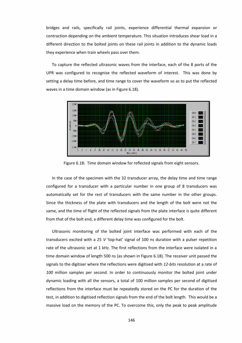
146

bridges and rails, specifically rail joints, experience differential thermal expansion or

contraction depending on the ambient temperature. This situation introduces shear load in a

different direction to the bolted joints on these rail joints in addition to the dynamic loads

they experience when train wheels pass over them.

To capture the reflected ultrasonic waves from the interface, each of the 8 ports of the

UPR was configured to recognise the reflected waveform of interest. This was done by

setting a delay time before, and time range to cover the waveform so as to put the reflected

waves in a time domain window (as in Figure 6.18).

Figure 6.18: Time domain window for reflected signals from eight sensors.

In the case of the specimen with the 32 transducer array, the delay time and time range

configured for a transducer with a particular number in one group of 8 transducers was

automatically set for the rest of transducers with the same number in the other groups.

Since the thickness of the plate with transducers and the length of the bolt were not the

same, and the time of flight of the reflected signals from the plate interface is quite different

from that of the bolt end, a different delay time was configured for the bolt.

Ultrasonic monitoring of the bolted joint interface was performed with each of the

transducers excited with a 25 V ‘top-hat’ signal of 100 ns duration with a pulser repetition

rate of the ultrasonic set at 1 kHz. The first reflections from the interface were isolated in a

time domain window of length 500 ns (as shown in Figure 6.18). The receiver unit passed the

signals to the digitiser where the reflections were digitised with 12-bits resolution at a rate of

100 million samples per second. In order to continuously monitor the bolted joint under

dynamic loading with all the sensors, a total of 100 million samples per second of digitised

reflections from the interface must be repeatedly stored on the PC for the duration of the

test, in addition to digitised reflection signals from the end of the bolt length. This would be a

massive load on the memory of the PC. To overcome this, only the peak to peak amplitude

147

values of each of the digitised reflection waves in the time domain window were selected and

stored on the PC. This amounts to 2.5 K samples per second, which is relatively small when

compared to 100 million samples per second. The digitised peak to peak amplitude values of

the reflected signals were recorded and streamed directly to the hard disk of the PC for post

processing. As explained in Chapter 3 of this thesis, the method described in this section and

applied in this study is a time domain approach.

Dynamic tests were carried out on the bolted joints with 8 transducer array and 32

transducer array. The bolted joint with 8 transducer array was designed to identify the peak

of contact pressure and show the difference in the clamping pressure away from the bolt

hole. Tests were only performed on the joint with a bolt torque of 50 Nm under an applied

cyclic shear load of 6 kN at a frequency 1 Hz. While for the specimens with array of 32

transducers, tests were performed on the bolted joint at a torque of 30, 40, 50 and 60 Nm

under an applied cyclic shear load of 6 kN at a frequency of 1 Hz. Furthermore, the joint was

subjected to varying cyclic shear loads of 5, 5.5, 6, 6.5, 7.0 and 7.5 kN at a frequency of 1 Hz

and bolt torque of 50 Nm. Tests were also performed on the bolted joint when it was

subjected to additional transverse side loads perpendicular to a constant cyclic shear load of

6 kN at a frequency of 1 Hz and bolt torque of 50 Nm. The value of the transverse side load

was held constant as the joint undergoes cyclic vibration during the test. Varying values of 1,

2, 3 and 4 kN of the transverse side loads were considered. For each of the tests, a washer

was placed under the bolt head and the length of the bolt was monitored ultrasonically to

determine the relaxation of tension in it during the test. The list of tests performed on the

dynamic bolted joints with the 32 transducer array is shown in Table 6.1

The transducer on the bolt head was similarly excited like other transducers and the

change in time of flight of the reflection echoed from the end of the bolt length was

monitored. To achieve this, the first reflection from the end of the bolt length was isolated in

a time domain window of length of 500 ns. The peaks of the reflection wave were located in a

time domain within the window, acquired and stored on the PC at a rate of 20 measured

samples per second during the test.

Prior to each test, a reference measurement of each of the sensors was recorded with the

bottom plate (i.e., plate B) absent. The reference measurement of the sensor on the bolt

head was also recorded when the bolt had not been tightened. The webcam was set to take

an image of the bolt head and top plate every second, and the images acquired were stored

on a PC. The stored ultrasonic data on the PC were later post-processed to determine the

148

dynamic reflection coefficient at the interface. The stored webcam images were also post-

processed to determine the angle of rotation during the test.

Table 6.1: Loosening tests performed on the dynamic bolted joints

Test number

Torque (Nm)

Cyclic Shear Load (kN)

Frequency (Hz)

Transverse Load (kN)

Torque

1 30 6.0 1 0

2 40 6.0 1 0

3 50 6.0 1 0

4 60 6.0 1 0

Cyclic shear load

1 50 5.5 1 0

2 50 6.0 1 0

3 50 6.5 1 0

4 50 7.0 1 0

5 50 7.5 1 0

6 50 8.0 1 0

Frequency

1 50 6.0 1 0

2 50 6.0 2 0

3 50 6.0 3 0

4 50 6.0 4 0

Transverse Load 1 50 6.0 1 0

2 50 6.0 1 1

3 50 6.0 1 2

4 50 6.0 1 3

5 50 6.0 1 4

6.6 Results

6.6.1 Loosening of joint with 8 transducer array

The dynamic reflection coefficient of the reflected ultrasonic signals from the interface for

each of the dynamic tests was calculated by dividing the reflected signal during the loosening

test by the reference signal. By doing this, the attenuation of signals in the plate material are

cancelled out. The dynamic reflection coefficient gives a measurement of relative contact

149

between the bolted plates and thus, the loosening of the joint during the cyclic loading.

According to equation 3.9, the relationship between the reflection coefficient and the

interfacial stiffness is inverse and the relationship between the interfacial stiffness and the

nominal contact pressure, for a low pressure, is linear (equation 3.10). Hence, an inverse

relationship exists between the reflection coefficient and nominal contact pressure.

Therefore, a value of dynamic reflection coefficients less than 1, indicates that the bolted

plates are in contact. As the value increases towards 1, the contact pressure between the

interfaces of the plates decreases, which implies that the plates are separating. A value of 1

indicates that the entire ultrasonic signal has been reflected from the interface because the

plates had separated and the contact pressure at the interface has become zero.

Figure 6.19: (a) Dynamic reflection coefficient measurement with oscillation effect, and

(b) Moving average of the dynamic reflection coefficient measurement.

Figure 6.19 shows the measured dynamic reflection coefficients from the 8 sensor array

when the test was performed on the joint with 50 Nm torque subjected to a cyclic load of 7

kN. Figure 6.19 (a) represents results of the raw data from the 8 sensor array that was

designed to identify the difference in the clamping pressure away from the bolt hole. The

figure shows changes in the measured reflection coefficient that are characterised by

oscillation in the measurement. The oscillation in the measurement of the dynamic reflection

coefficient is due to the relative movement between the ultrasonic sensors and the bolt head

(a)

(b)

150

as a result of the displacement cycles forced upon the joint as shown in Figure 6.20, and the

frequency of the oscillation of the signal corresponds to the frequency of the vibration of the

bolted joint. As observed earlier under the static scanning of bolted joints in chapter four,

the pressure distribution at the interface is dictated by the bolt head. It is clear that when

the joint is properly aligned before oscillation, as in the Figure 6.20 (a), the sensor receives

signal from the highest contact pressure point and consequently a low reflected signal. Once

the vibration started, as shown in Figures 6.20 (b) and (c) with a display of exaggerated

bending of the bolt, the joint undergoes dynamic displacement and the plates move relative

to each other. This caused the position of the sensor bonded to the back of the lower plate to

move relative to the bolt head, and also to the contact pressure distribution. As a result of

this, the sensor measured different points of the contact pressure distribution.

Figure 6.20: Relative position of the sensor and the contact pressure distribution (a) when

joint components are aligned (b) when the components moved due to a

tensile force of the joint (c) when the components moved due to a

compressive force of the joint.

As mentioned earlier, the oscillation on the dynamic reflection coefficient data is a

measurement effect that occurs at a frequency which corresponds to that of the vibration of

the bolted joint, and in order to remove the oscillation effect so as to permit meaningful

analysis of results, the data were processed using a simple moving average technique. Using

the simple moving average technique, a series of averages of different subsets of the full data

set were calculated to obtain the centre point of the measurements and this smoothed the

151

oscillation effect caused by the vibration of the joint. Figure 6.19 (b) shows changes in the

measured dynamic reflection coefficient without the oscillation effect in the measurement.

From the figure, the initial values of the dynamic reflection coefficient for sensors 1, 2, 3 and

4 located at a distance of 7 mm from the bolt hole on the plate specimen were 0.539, 0.589,

0.628 and 0.631 respectively, and the values of 0.685, 0.760, 0.781 and 0.826 were recorded

for sensors 5, 6, 7 and 8 that were located at a distance of 8 mm, 9 mm, 10 mm and 11 mm

from the centre of the bolt hole respectively. Sensors 1, 2, 3 and 4 that were close to bolt

hole show lower values, and hence higher contact pressure, when compared to the sensors

that were further from the bolt hole. This is an indication that the initial value of the

reflection coefficient increases as the relative distance between the sensors and the bolt hole

increases. Since the value of of the dynamic reflection coefficient shows the relative contact

between the bolted plates, this partly indicates that the sensors are working well and more

importantly, it confirms that the contact pressure decays from the edge of the bolt hole as

observed under the scanning of static bolted joints.

Furthermore, it can be seen that for all the sensors, the value of reflection coefficient

increases rapidly from its initial value, and then followed by a gradual increase in value to an

approximate value of 1 during the vibration cycle. This shows that high percentage of the

preload and thus, contact pressure was rapidly lost followed by gradual loss of the remaining

preload as the loosening of the joint took place during the test. It can also be observed that

no matter the initial value of the measured dynamic reflection coefficient, the time for each

of the dynamic reflection coefficients of the sensors to attain the approximately value of 1

are almost the same. This indicates that although the contact pressure distribution at the

interface may not be the same, that as the joint lose preload, the contact pressure

distribution over the entire interface also reduce in proportion until the interface separates

at almost the same time. Since the bolted joint with 8 transducer array was designed to

identify the difference in the clamping pressure away from the bolt hole, most of the

discussions on the dynamic bolted joint tests will come up under the results of the joint with

the 32 transducer array which gives more resolution.

As mentioned earlier, the relaxation of tension in the bolt was equally monitored by

observing the change in length of the bolt during the vibration tests using the time of flight of

the ultrasonic signal. Time of flight is the time taken for ultrasonic signal to travel from a

transducer to a targeted partially reflective surface and back again. Therefore, the change in

length of the bolt was determined by monitoring the time of flight for an ultrasonic signal to

travel to-and-fro between the bolt head and the end of the bolt length. A typical dynamic

152

time of flight measurement of the joint at a bolt torque of 50 Nm is shown in Figure 6.21. The

figure, like dynamic reflection measurement, shows changes in the measured dynamic time

of flight characterised by the oscillation in the measurement as the bolt length reduces. The

oscillation in the measurement was as a result of relative movement between the ultrasonic

sensor bonded to the head of the bolt and the end of the bolt length due to the displacement

cycle forced on the joint as shown in the exaggerated diagram in Figure 6.22. The frequency

of the oscillation in the measured time of flight also corresponds to the frequency of the

vibration of the bolted joint.

Figure 6.21: A typical dynamic time of flight measurements at 50 Nm bolt torque.

From the figure, it is clear that the sensor received signal from the mid of the centre of the

threaded length of the bolt when the joint was properly aligned. But once the vibration

started, the joint undergoes dynamic displacement and the bolt bent as the plates move

relative to each other (as shown in (b) and (c) of the Figure 6.22). This caused the position of

the sensor bonded to the head of the bolt to move relative to the centre of the threaded

length of the bolt and thus it received signals from the points of relatively different length

from the centre of the threaded length of the bolt due to the bending of the bolt.

Furthermore, as the joint relaxed the bending of the bolt will increase, the relative distance

between points from which sensor received signal also increase and this caused the increase

in the amplitude of the oscillation. As the tension in the bolt relaxes and the length of the bolt

reduce, these points at the end of the bolt also reduce accordingly, thus indicates an overall

relaxation of tension in the bolt. For the reason of meaningful presentation and analyses of

data, the aforementioned simple moving average technique was used to extract the centre

points of the measurement of the reduction in the dynamic time of flight. This represents the

reduction in length of the bolt during the test, will be presented from now on.

153

Figure 6.22: Relative position of the sensor and the end of the bolt end.

The results of the measured dynamic reflection coefficient of the 32 sensor array were

also characterised by the oscillation in the measurement which is similar to the observations

in Figure 6.19 (a), and this is due to relative movement between the ultrasonic sensors and

the bolt head as the joint undergoing displacement cycles forced on it during the cyclic

loading. Therefore, for the purpose of meaningful presentations and analyses of the results,

the experimental data were equally processed using a simple moving average technique to

obtain processed results similar to that of Figure 6.19 (b). Hence, from this point onward the

processed data from a moving average technique of the test results will be presented.

6.6.2 Loosening of joint with 32 transducer array

Figure 6.23 shows typical results of measured dynamic reflection coefficient from the

bolted joint with 32 sensor array. The joint was torqued up to 50 Nm and subjected to cyclic

loads of 6 kN at a frequency of 1 Hz. The figure shows the result of measured reflection

coefficient in four groups of eight sensors as indicated in the sensor layout in Figure 6.4. In

Figure 6.23, it can be observed that the values of dynamic reflection coefficient of sensors

with the same numerical identity in all the groups did not start at the same initial values (e.g.,

sensor 1 had initial values 0.44, 0.36, 0.50 and 0.32 in group A, B, C and D respectively). This

can be attributed to the effect of non-uniform clamp from the bolt head as a result of the

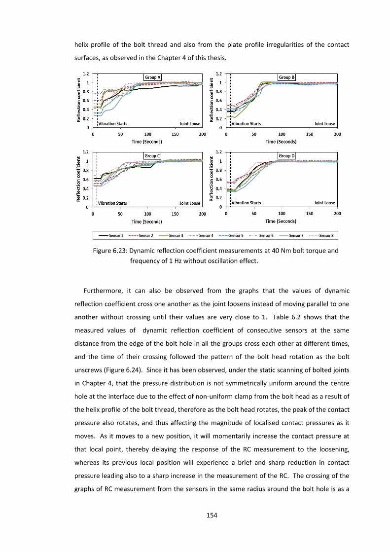
154

helix profile of the bolt thread and also from the plate profile irregularities of the contact

surfaces, as observed in the Chapter 4 of this thesis.

Figure 6.23: Dynamic reflection coefficient measurements at 40 Nm bolt torque and

frequency of 1 Hz without oscillation effect.

Furthermore, it can also be observed from the graphs that the values of dynamic

reflection coefficient cross one another as the joint loosens instead of moving parallel to one

another without crossing until their values are very close to 1. Table 6.2 shows that the

measured values of dynamic reflection coefficient of consecutive sensors at the same

distance from the edge of the bolt hole in all the groups cross each other at different times,

and the time of their crossing followed the pattern of the bolt head rotation as the bolt

unscrews (Figure 6.24). Since it has been observed, under the static scanning of bolted joints

in Chapter 4, that the pressure distribution is not symmetrically uniform around the centre

hole at the interface due to the effect of non-uniform clamp from the bolt head as a result of

the helix profile of the bolt thread, therefore as the bolt head rotates, the peak of the contact

pressure also rotates, and thus affecting the magnitude of localised contact pressures as it

moves. As it moves to a new position, it will momentarily increase the contact pressure at

that local point, thereby delaying the response of the RC measurement to the loosening,

whereas its previous local position will experience a brief and sharp reduction in contact

pressure leading also to a sharp increase in the measurement of the RC. The crossing of the

graphs of RC measurement from the sensors in the same radius around the bolt hole is as a

155

result of this momentarily variation in contact pressure at the interface as the peak of the

contact pressure moves over it, as the bolt head rotates during loosening.

Sensors Time Sensors Time

D5 & D1 25.3 D7 & D3 23.8

D1 & C5 44.0 D3 & C7 -

C5 & C1 48.8 C7 & C3 50.5

C1 & B5 49.0 C3 & B7 46.0

B5 & B1 50.4 B7 & B3 49.0

B1 & A5 51.0 B3 & A7 50.5

A5 & A1 56.9 A7 & A3 53.4

To eliminate the effects due to the thread profile and other plate irregularities, the

average of the measured dynamic reflection coefficient of the sensors in each ring and for all

the rings (i.e., from the inner ring to the outer ring) was calculated for each of the tests

performed, and the results of the tests on varying torques, cyclic shear loads, transverse

shear load and frequency are presented in the following sections.

6.6.3 Bolt torque and cyclic shear load

Figure 6.25 (a) shows the results of the tests performed on the bolted joint at a torque of

30, 40, 50 and 60 Nm under an applied cyclic shear load of 6 kN at a frequency of 1 Hz.

While the tests performed on the bolted joint of 50 Nm bolt torque at a varied cyclic shear

load of 5.5 kN, 6 kN, 6.5 kN, 7 kN, 7.5 kN and 8 kN at a frequency of 1 Hz is shown in Figure

6.25 (b). These results show the dynamic reflection coefficient, dynamic reduction in time of

flight and the rotation of the bolt head during the tests. Similar to the observation in the

results of 8 transducer array, it can be seen from the figure that as the bolted joints loosening

the value of the dynamic reflection coefficient increases rapidly from its initial value and then

followed by a gradual increase in value to approximately value of 1 during the vibration

cycles. The values of the reduction in dynamic time of flight, which represents the relaxation

of the tension in the bolt and the values of the rotation of the bolt head during the tests all

Table 6.2: Time when the measured dynamic

reflection coefficient cross

Figure 6.24: Direction of the bolt head rotation

during loosening relative to the sensors.

156

increase rapidly from their initial values of almost zero to approximately uniform values as

the bolted joints loosening.

Furthermore, it can be seen that different values of the initial value of the dynamic

reflection coefficient were recorded for the various bolt torques, and these measurements

decrease as the value of the bolt torque increases. This could be attributed to the fact that

more asperity contacts were made at the interface as additional load is being applied through

the tightening of the bolt. Therefore, as the load increases, more and more signals are

transmitted at these new asperity junctions thereby reducing the proportion of the signal

sent that was reflected.

157

Figure 6.25: (i) Dynamic reflection coefficient, (ii) reduction in time of flight and (iii)

rotation of the bolt head measurements at various (a) torques and (b)

cyclic shear loads.

(a)

(b)

(i)

(ii)

(iii)

(i)

(ii)

(iii)

158

It can also be seen from the figure that the measured reduction in the dynamic time of

flight attains an approximately uniform value at different values of 0.10 ns, 0.12 ns, 0.16 ns

and 0.21 ns for torque of 30, 40, 50 and 60 Nm. This indicates that the bolt experienced

more tension, and thus stretches more, as the bolt torque increases. While in the case of the

of cyclic shear loads (Figure 6.25 (b)), it can be seen that the initial values of dynamic

reflection coefficient are similar for all the cyclic shear loads measured, and also the dynamic

time of flight attains approximately the same value at the end of the loosening. This was

because the same value of bolt torque of 50 Nm was applied in all the loads considered. The

same fact also relates to the rotation of the bolt head where the values of the total rotation

are similar in the test of the cyclic shear loads as compared to that of the varying bolt torques

at the end of the joints loosening. This is because the angle turned by the bolt head during

tightening of the bolt of the joint was not the same for the different torques applied, which

was similar in the case of cyclic shear loads.

In Figure 6.25 (a), the calculated average dynamic reflection coefficient attained the value

of almost 1 at approximately 100.2 seconds, 158.3 seconds, 172.9 seconds and 183.4 seconds

at bolt torque of 30 Nm, 40 Nm, 50 Nm and 60 Nm respectively. This indicates that the time

for complete loosening of bolted joints to occur increases as the applied bolt torque

increases. The results of dynamic reduction in time of flight as well as the results of the

monitored rotation of the bolt head during the vibration tests also show that the time for a

complete relaxation of a given joint to occur decreases as the applied bolt torque increases.

As can be seen, the measured reduction in the dynamic time of flight reaches approximately

uniform value of 0.10 ns, 0.13 ns, 0.18 ns and 0.24 ns at 55.4 seconds, 64.8 seconds, 75.9

seconds and 110.1 seconds for the bolt torque of 30 Nm, 40 Nm, 50 Nm and 60 Nm

respectively, while a time value of 134.0 seconds, 154.0 seconds, 167.0 and 195.0 seconds

was recorded for bolt torque of 30 Nm, 40 Nm, 50 Nm and 60 Nm respectively at the

commencement of the approximately steady state of the rotation of the bolt head.

It can be seen in Figure 6.25 (b), which shows the results of varied cyclic shear load, that

the time at which the bolted joint attained complete relaxation decreases as the applied

cyclic shear load increases. The average dynamic reflection coefficient measurements

attained the value of 1 at approximately 143.7 seconds, 72.1 seconds and 54.6 seconds for

the cyclic shear loads of 6 kN, 7 kN and 8 kN respectively. Also, the time taken for the

measured dynamic reduction in dynamic time of flight and the bolt head rotation to attain

the approximately uniform value decreases as the dynamic shear load increases. A time

value of 107.2 seconds, 65.22 seconds and 41.3 seconds was recorded for the dynamic

159

reduction in dynamic time of flight, while a time of 170.0 seconds, 98.0 seconds and 68.0

seconds was recorded for the rotation of bolt head of the respective dynamic shear load of 6

kN, 7 kN and 8 kN as the time they approximately attained uniform values. These results

show that the rate at which complete relaxation occurs increases as the applied dynamic

shear load increases.

6.6.4 Transverse side load and frequency

Figure 6.26 (a) shows the result of tests performed on the bolted joint with a torque of 50

Nm and subjected to additional transverse side loads, perpendicular to a 6 kN cyclic shear

load at a frequency of 1 Hz, and Figure 6.26 (b) shows the results of the tests performed on

the bolted joint of 50 Nm bolt torque at four different frequencies of 1, 2, 3 and 4 Hz. The

figure shows the results of the dynamic reflection coefficient, the reduction in time of flight

and the rotation of the bolt head with features that characterised loosening of bolted joints

which have been observed in the results of the previous tests. In addition to these features,

as shown in Figure 6.26 (a), the measured dynamic reflection coefficient reaches a value of 1

at approximately 128.2 seconds, 97.7 seconds, 92.6 seconds, 88.7 seconds and 78.6 seconds

for transverse loads of 0 kN, 1 kN, 2 kN, 3 kN and 4 kN respectively. Since the time for the

value of the dynamic reflection coefficients to reach the value of 1 reduces as the value of

transverse side load increases, it indicates that additional transverse load acting in a

perpendicular (or other directions) to the direction of the cyclic shear load will increase the

rate at which relaxation occurs in a bolted joint, and an increase in the value of this additional

applied transverse load will also increase the rate of relaxation in a joint.

Furthermore, the results relaxation of tension in the bolt and the rotation of the bolt head

during the tests show that there was a steady reduction in the time of loosening as the

transverse load increases. A time value of 109.2 seconds, 95.6 seconds, 84.1, 72.8 and 64.7

seconds was recorded at the transverse side load of 0 kN, 1 kN, 2 kN, 3 kN and 4 kN

respectively at the end of the rapid increase in value of the measured dynamic reduction in

time of flight. While rotation of the bolt head during the tests attains an approximately

steady state at a time of 168.0 seconds, 122.0 seconds, 114.0, 106.0 and 86.0 for the

transverse shear load of 4 kN, 3 kN, 2 kN, 1 kN and 0 kN respectively. These are also an

indication that the rate at which complete loosening occurs increases as the applied

transverse shear load increases.

160

Figure 6.26: (i) Dynamic reflection coefficient, (ii) reduction in time of flight and (iii)

rotation of the bolt head measurements at various (a) transverse shear loads and

(b) frequencies.

(a)

(b)

(i)

(ii)

(iii)

(i)

(ii)

(iii)

161

Figure 6.26 (b) shows the effect of variation in loading frequency on the loosening of

bolted joints. It can be seen that the time for complete loosening of the bolted joint to occur

in the measured dynamic reflection coefficient, dynamic reduction in time of flight and

rotation of the bolt head during the tests decreases as the frequency of the applied dynamic

shear load increases. The dynamic reflection coefficient measurements reach a value of 1 at

approximately 114.7 seconds, 66.6 seconds, 42.0 seconds and 36.0 seconds for a frequency

of 1 Hz, 2 Hz, 3 Hz and 4 Hz respectively. This shows that the time taken for complete

loosening of the joints almost reduced to half as the frequency of vibration increases from 1

Hz to 2 Hz. Also, as the frequency double from 2 Hz to 4 Hz, the time taken to reach a value of

1 at a vibrating frequency of 3 Hz falls middle of the values of measured reflection coefficient

2 Hz and 3 Hz frequencies.

The time of flight increases rapidly from a value of 0 to approximately 0.15 ns at a time of

79.4 seconds, 62.8 seconds, 30.2 seconds and 17.7 seconds before giving way to a more

steady increase state for the frequency of 1 Hz, 2 Hz, 3 Hz and 4 Hz respectively. While the

time taken for the rotation of the bolt head to reach the end of the rapid increase reduced

from 178 seconds to 91 seconds, 85 seconds and 72 seconds as the frequency increase from

from 1 Hz to 2 Hz, 3 Hz and 4 Hz respectively. Certainly, these also imply that the time taken

for complete loosening of bolted joints increases as the frequency of the applied dynamic

shear load increases.

As the time taken from the joint to completely lose its preload reduces as the frequency

increases, the number of cycles for loosening of joint to occur also increases with the

increasing frequency. Therefore, since the number of cycles is doubled as the frequency

increases from 1 Hz to 2 Hz and the time taken for the joint to loosen reduces approximately

by half (as shown in the results), it implies that the loosening of bolted joints is a function of

the number of cycles of loading rather than frequency (provided there are no resonant

effects). This is in agreement with Pai and Hess [57] that loosening rate is independent of

frequency of the applied load.

6.7 Discussion

The results from the applied cyclic shear load can be related to real life situations like a

train going across a joint in the rail. As the speed of the passing train increases, the frequency

of the shear loading on the joint also increases as the wheels will pass the rail joint at a closer

interval. If the axle load due to the weight of the train increases the cyclic shear loading on

the joint also increases. The effect of thermal stress due to variation in temperature will be

an additional shear load on the joint which is perpendicular to the axle load from the train.

162

The effect of non-uniform clamping from the bolt head as a result of the helix profile of

the bolt thread and also from the plate profile irregularities of the contact surfaces can be

observed in the results of the 8 transducer array and also in the results of other tests from

the 32 transducer array. Sensor 1, 2, 3 and 4 were mounted equidistant from the edge of

the bolt hole, so as to enable the peak contact to be measured. It is expected that the

measured values of reflection coefficient would be the same, but there is variation in the

observed values and this can be majorly attributed to the unbalanced contact pressure at the

contact interface due to the above mentioned reasons. Furthermore, as shown in Table 6.2

and Figure 6.24, the position of the this imbalance, as the bolt unscrewed, was observed to

move with the rotation of the bolt head, especially before a high percentage of the joint

preload was expended. Since it has been observed that the position of the peak of the

contact pressure at the interface varies as the bolt head rotates during tightening [76], the

location of the peak, attributed to the imbalance in the contact pressure at the interface due

to the effect of the profile of thread on the bolt, will likewise move in the direction of the bolt

head rotation when the bolt unscrews during loosening.

6.7.1 Features of the results profile

In all the results from the monitoring of relaxation of contact pressure at the interface, the

graphs of the results show almost identical features. Taking the result of the dynamic shear

load of 5.5 kN at a frequency of 1 Hz as an example (shown in Figure 6.27), it can be seen that

the value of dynamic reflection coefficients which measures the relative contact between the

interface of bolted plates and thus, the loosening of the joint during the cyclic loading

increases from a value of less than 1 when the bolted plates were in contact to a value of 1

when they were separated. While during the same period the result shows that the

reduction in time of flight, which represents the change in length (reduction in length) as the

tension in the bolt relaxes during the loosening of the bolted joint increases from initial value

0 to almost 0.19 ns.

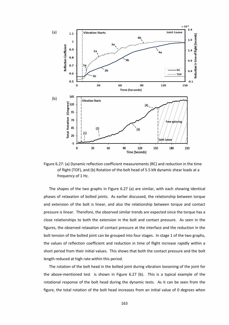
163

Figure 6.27: (a) Dynamic reflection coefficient measurements (RC) and reduction in the time

of flight (TOF), and (b) Rotation of the bolt head of 5.5 kN dynamic shear loads at a

frequency of 1 Hz.

The shapes of the two graphs in Figure 6.27 (a) are similar, with each showing identical

phases of relaxation of bolted joints. As earlier discussed, the relationship between torque

and extension of the bolt is linear, and also the relationship between torque and contact

pressure is linear. Therefore, the observed similar trends are expected since the torque has a

close relationships to both the extension in the bolt and contact pressure. As seen in the

figures, the observed relaxation of contact pressure at the interface and the reduction in the

bolt tension of the bolted joint can be grouped into four stages. In stage 1 of the two graphs,

the values of reflection coefficient and reduction in time of flight increase rapidly within a

short period from their initial values. This shows that both the contact pressure and the bolt

length reduced at high rate within this period.

The rotation of the bolt head in the bolted joint during vibration loosening of the joint for

the above-mentioned test is shown in Figure 6.27 (b). This is a typical example of the

rotational response of the bolt head during the dynamic tests. As it can be seen from the

figure, the total rotation of the bolt head increases from an initial value of 0 degrees when

(a)

(b)

164

the bolted joint components were still in contact to a fairly steady maximum value when the

joint as loosened. Similar to the measured relaxation of tension in the bolt and relaxation of

contact pressure at the plate interface, the stage of loosening can also be grouped into four

stages. However, no significant change in value was recorded in the stage 1 of the rotation of the bolt

head..

6.7.2 Phases of loosening

As shown in the discussion above, loosening of bolted joints exhibits phase changes that can be

grouped into four stages: an initial very rapid loosening (stage 1), followed by less rapid loosening

(stages 2 and and 3) and lastly, a gradual loosening Stage (stage 4). The loosening process could be

compared to the illustration by Bickford [24] of the sequence by which shear joint fails in response to

external loads (Figure 13(a)): the first stage involves elastic deformation of the bolted joint

components, followed by the clamped components slipping relatively to one another, leading to

greater interaction with the bolt after the friction at the interface has been overcome. Next additional

elastic and plastic deformation occur respectively, before eventual failure. In the case of loosening due

to dynamic shear load (Figure 13(b)), stage 1 involves a quick reduction of tension in the bolt and fast

separation of the clamped interface, and this could be attributed to a rapid slip between the threads of

the bolt and that of the mating component.

Figure 13: (a) Illustration of the sequence by which shear joint fails in response to external loads

[24] and (b) Four-stage self-loosening sequence of bolted joints in the present study.

The value of reflection coefficient and reduction in time of flight increases less rapidly in stage 2

and stage 3. The interactions between the clamped members and the bolt increased in this stage. This

introduced further bending of the bolt and the gross slip at the bolt head, and the consequent rotation

of the bolt head (as shown in Pai and Hess [57]). Once the friction at the interfaces have been

overcome due to a substantial relaxation of the bolt tension and contact pressure at the interface, the

effect of the dynamic shear force, assisted by the thread profile, is more concentrated on unscrewing

the bolt in the later part of this stage. This also corresponds to stage 2 and stage 3 under the rotation

of the bolted head (Figure 12(b)) where there is a gradual and later rapid increase in rotation. This

stage also is the same as stages 2 and 3 under the Bickford illustration. At the end of stage 3, the

165

results show that a high percentage of the joint preload has been lost. The last phase of the loosening

process (stage 4) exhibited a gradual increase in the measured values. This phase compensates for the

effect of the rundown of the bolt and alignment of the members during the tightening process of the

bolted joint.

.

.

The sequence of loosening of bolt joints as described above can also be seen, but in

reverse order, in the typical curve of general modelling of tightening process (Figure 6.29) of

fastener in bolted joint presented by Ralph et al. [167]. The zoned 4 corresponds to stage 1 in

the present work where no (insignificant) rotation of of bolt head was observed. Zone 3, 2

and 1 correspond to stage 2, 3 and 4 of the present study respectively.

Figure 6.28: Applied torque vs rotation of the nut or bolt [167].

6.7.3 Initiation of loosening and ratchetting

The measurements of the percentage of the total joint loosening of the three areas of the

bolted joint in the first 30 seconds of the vibration test show that the loosening of the joint

started at different times (Figure 6.30). According to the figure, at 5 seconds after the

commencement of the test, no loosening is indicated from the three areas. At 10 seconds,

the change in the monitored tension (TOF) in the bolt shows an appreciable 4 % loosening,

while the result of the change in the contact pressure (RC) indicates that 0.6% of the total

loosening has occurred, and no rotation of the bolt head is observed. A total loosening of

0.1% is noticed in the bolt head at 20 seconds after the start of the test, while an appreciable

loosening of 2% was recorded at 25 seconds at the time when TOF and RC indicated that half

and one fifth of the total loosening have been accomplished.

166

Figure 6.29: Dynamic reflection coefficient, reduction in time of flight and rotation of

the bolt head measurements in the first 30 seconds of vibration test.

This observation is in agreement with the earlier observations by some authors. Junker

[51], Izumi et al. [66] and Pai and Hess [56] had observed in the experimental studies of

loosening of fasteners in bolted joints under shear loading, that fastener threads generally

slip before complete slip of the bolt head. Yanyao Jiang et al. [63] revealed that the early

stage of self-loosening in bolted joint is characterised by a short and sharp clamping force

reduction with no relative rotation between the nut and the bolt. They believed that the early

stage of self-loosening is caused by localized cyclic plastic deformation (cyclic strain

ratcheting) of the bolt which caused a redistribution of stresses in the bolt and resulted in the

gradual loss of clamping force with loading cycles. The present experimental results show

that when bolted joint is subjected to cyclic shear loading, the fastener threads generally slip

first, followed by separation of the interface of the bolted components and lastly, by the

gross slip (rotation) of the bolt head. Since in the first 15 seconds, no rotation of the bolt

head was observed while changes in the bolt tension and interface contact pressure of the

bolted joints have indicated loosening in the bolted joint, it implies that the early stage of the

loosening of bolted joint is actually characterised by cyclic strain ratcheting. Moreover, the

observed cross of the values of the dynamic reflection coefficient (Figure 6.23 and Table 6.2)

which is due to movement of the peak of the contact pressure started after 23 seconds. This

also shows that the observed phenomenon is usual due to rotation of the head, and that

cyclic strain ratcheting actually occurred because no appreciable rotation of the bolt head

happened before that time.

6.7.4 Differential loosening rates across the interface

The loosening in the present context implies the change in value of the dynamic reflection

coefficient from the initial value at the start of a test when bolted plates are in contact and some

portion of the ultrasonic signal is transmitted through the contact interface (i.e. 0 % loosening) to

167

when the value is 1 which indicates that the entire ultrasonic signal has been reflected from the

interface because the plates had separated (i.e. 100 %loosening). Hence, mid value between the initial

value and the value of 1 of the dynamic reflection coefficient indicates 50% of loosening.

Therefore, the time for the joint to lose 50% and 90% of its contact pressure at different

radial distances on the bolted interface, and also at various torques, is shown in Figure 6.31.

1st, 2nd, 3rd and 4th represents the average of dynamic reflection coefficient measured by the

sensors at radial distance of 7 mm, 8 mm, 9 mm and 10 mm from the bolt centre respectively

(as shown in Figure 6.4).

Figure 6.31 shows that the rate at which loosening occurs over the bolted joint interface

vary. It can be observed that in all cases, sensors at a distance of 10 mm attained 50% and

90% of the loosening phases some seconds before sensors at distance 7 mm from the bolt

centre. This time lapse is greater at 90% than at 50% of the loosening. The reason for this is

due to the unequal clamping pressure at the interface as observed under the scanning of the

static bolted joint in the chapter 4 of this thesis. The decrease of the clamping pressure with

distance away from the bolt hole allows the areas with lower pressure to slip and loose

before the regions with higher contact pressure. This is supported by the theory of localised

slip submitted by Chesson and Munse [54] and Hemmye [55] which states that slip, at the

onset of loosening, always start at some distance away the bolt hole and migrate towards

bolt hole. The present study shows that the rate of loosening at the bolted joint interface are

also not the same, but increases away from the bolt hole.

Figure 6.30: Dynamic reflection coefficient measurements at different radial distances of

the bolted contact interface.

Figure 6.32 shows the time for the joint to lose 50% and 90% of its integrity as monitored

from the three parts of the bolted joints for the various torques, frequencies, axial loads and

168

side loads. In all the tests, the time for the bolt to attain these percentages of loosening as

measured by the change in time of flight (TOF) is fastest, followed by the time the interface

recorded these percentage loses in its contact pressure as measured by the dynamic

reflection coefficient. The figure shows that the time for the bolt head to attain these

percentages of loosening through rotation during the vibration loosening was more than the

other two. This indicates that the rate of loosening of these three major components of

bolted joint is not the same. As also observed and explained in the Section 6.5.3, this is partly

due to the early stage of the self-loosening caused by cyclic strain ratcheting of the bolt which

caused changes in the length of the fastener (bolt) and thus loosening without rotation of the

bolt.

6.7.5 Effect of bolt torque

As shown in the Figure 6.32 (a), the results of the change in time of flight, dynamic

reflection coefficient measurements and the rotation of the bolt head show that the rate of

loosening of bolted joint under cyclic loading decreases as the applied bolt torque increases.

Just like observations from most of the earlier studies [51, 53, 57, 76] on the loosening of

bolted joints, these results shows that the resistance of the bolted joints to vibration

loosening increases as the applied bolt torque increase. However, it can be observed that the

rate of increase in the dynamic reflection coefficient and change in time of flight at the early

stages, stage 1 and stage 2 of relaxation of contact pressure at the interface during loosening

reduces as the torque increases (Figure 6.25 (a), the slope of the results reduces with the

increase in the torque at the period). This shows that the longer it takes for the cyclic shear

load to overcome the stages 1 (which is mostly characterised by cyclic strain ratcheting) and

part of stage 2, the lower the loosening rate and the better is the resistance of the bolted

joint to vibration induced loosening. The higher tightening torque caused the joint preload

and the frictional force at the thread to increase, and thereby increased the resistance of the

fastener to slip (cyclic strain ratcheting) at the thread interface as a result of shear load.

Furthermore, the difference between the change in time of flight, dynamic reflection

coefficient measurements and the rotation of the bolt head at 50% and 90% loosening

follows the same trend as the torque increases. Hence, it shows that the rate of loosening of

bolted joint depends on tightening torque, but the process of loosening is independent of the

tightening torque. In addition, the initial value of the dynamic reflection coefficient

measurements decreases as the value of the applied bolt torque increases (Figure 6.25 (a)).

Since measurements are taken from discrete points at the interface, the decrease in the

169

initial value of the dynamic reflection coefficient measurements as the value of the applied

bolt torque increases shows that more asperity contacts are made at the discrete points of

the interface as additional load is being applied through the tightening of the bolt thereby

reducing the proportion of the signal sent that was reflected. This supported earlier

observation under the scanning of static bolted joints in chapter four that additional load is

supported by a highly clamped area of the contact zone as more load is being applied through

the tightening of the bolt.

170

Figure 6.31: Dynamic reflection coefficient, reduction in time of flight and rotation of the bolt

head measurements at 50% and 90% of loosening life for the various (a) torques

(b) frequencies (c) cyclic shear loads and (d) transverse shear loads.

50% TOF

50% RC

50% Rot

90% TOF

90% RC

90% Rot

(a)

(b)

(c)

(d)

171

6.7.6 Effects of frequency

When a joint is sufficiently preloaded at higher torque, the bolt tension and contact

pressure at the interface are equally high. Hence, the cyclic shear load needs to be applied

for a longer period to overcome friction and initialise slips at the interfaces. However, at a

higher frequency the bolt experienced more cycles of cyclic shear loading in the same time

interval, and consequently, the relaxation of the joint should be faster. Therefore, as shown

in the Figure 6.32 (b), the three methods used to monitor the relaxation of the bolted joints

show a proportional decrease in the time taken for relaxation to occur as the frequency

increases. This shows, like observations from Baubles et al. [168] and Pai and Hess [56], that

frequency may affect the time of loosening of bolted joints as a result of number of induced

vibration, but loosening rate is independent of frequency of the applied load.

However, apart from the observed general reduction in the time at which loosening is

accomplished as the frequency increases, the profile graphs (Figure 6.26 (b)) of the frequency

show that as the frequency increases the time to achieve all the stages of loosening equally

increases. As seen in the figure, the slope of the results of the dynamic reflection coefficient

and change in time of flight continues to increase (becomes steeper) as the value of the

frequency of the loading cycle increases, and the stage II of the loosening process becomes

increasingly indistinguishable as the stage is accomplished faster. The results profile of the

rotation of the bolt head also shows a continuous increase in the rate of loosening, especially

at the stage II (steeper slope of the profile), as the frequency of the loading cycle increases.

This corresponds to part of stage II and stage III of the dynamic reflection coefficient and

change in time of flight profiles. Once the preload in the fastener is reduced as a result of the

increasing cyclic strain ratcheting in stage I, the reduction or absence of the period for stage II

of the loosening process implies that the friction between the clamped components become

easier to overcome as the frequency increases. The slip and the rotation of the bolt head

correspondingly increases as the frequency of cyclic loading increases.

6.7.7 Effect of cyclic shear load

The rate of loosening of bolted joints increases as the applied cyclic shear load increases,

as shown in the results section and also Figure 6.32 (c). When a joint is preloaded, the

stiffness of the joint, the bolt tension and consequently the contact pressure at the interface

are maintained by the frictions at the interface. If sufficient cyclic shear load to overcome

these frictions at the contacts is applied, there will be slip at the thread, bolt head and plate

172

interfaces, and hence loosening will occur. The rate at which slip occurs in the early stages

and the consequent loosening depends on the magnitude of the shear load. As can be seen

in the results profile of the dynamic reflection coefficient and reduction in time of flight

(Figure 6.25 (b)), the rate of loosening increases at the early stages of relaxation of bolt

tension and contact pressure at the interface as the applied cyclic shear load increases. In the

figure, the profile graph of the measured dynamic reflection coefficient clearly shown that

the slope of the results increases with an increase in the dynamic shear load which implies

faster loosening of the bolted joints. Since this period corresponds to the period of non-

rotational loosening. This is an indication that the magnitude and the rate at which cyclic

strain ratcheting at occurred the threaded contribute to loosening depends on the amplitude

of the cyclic shear load. Most studies employed the amplitude of displacement of the cyclic

vibrating load, which is directly related to the magnitude of the vibrating load, to investigate

the vibrating induced loosening in bolted joints. Yanyao et al. [63] in their study showed that

an increase in the amplitude of displacement of the vibrating shear load increases the rate of

loosening in the early stage of self-loosening of bolted joints. Junker [51] and, Pai and Hess

[56] have also made the assertion that loosening depends on the amplitude of the applied

load. The present study also supported these statements, and shows that the higher the rate

of relaxation at the early stage of loosening due to increase in the magnitude of the vibrating

shear load, the lower is the resistance of the bolted joint to vibrating induced loosening in

bolted joints.

6.7.8 Effect of transverse side load

The most apparent cause of slip at the interface which is also responsible for loosening of

bolted joints is the shear load. When the resistance of the friction at the interface is

overcome by the shear load in one direction, any additional shear load in another direction

that is not opposing the direction of the first one will further reduce the remaining frictional

resistance at the interfaces. The results of the transverse side load show this to be true.

When an additional shear load is constantly applied to the joint in a perpendicular direction

to the dynamic shear load, it increases the rate of loosening of the joint. The results in Figure

6.32 (d) show that as the magnitude of the constant shear load increases, the rate of

loosening also increases even when the amplitude of applied cyclic shear load is constant.

In addition to the overall observed increase in the rate of loosening displayed by the

introduction of transverse shear load, Figure 3.26 (b) shows that the effect of introducing and

increasing the transverse shear load is more pronounced on the stage 2 than any other stages

173

of dynamic reflection coefficient and change in time of flight profiles. With the increase in the

shear load, there is almost absence of stage 2 as the stage is accomplished within a very short

duration; thereby making the start of stage 1 to the end of stage 3 appears continuous. This

shows that once the stage I is accomplished the side load help to free the clamped

components of frictional force at the interfaces very fast, and the rate at which the

movement (slip) at the clamped interface and bearing surface of the bolt head occurs

depends on the magnitude of the transverse shear load. Subsequently, the bearing of the

clamped component on the fastener introduced bending [56] and this helped in initiating

rotation of the bolt head and allow stage III to commence very early. The side load also assists

in the rotation of the bolt even after the separation of the clamped components has occurred

at the interface. This is also due to the additional bending effect on the bolt as a result of the

bearing of the clamped component on the bolt, which helps in the slip of the bolt head in

loosening direction.

Research studies have been conducted by several authors on the loosening of bolted

joints. In these studies, efforts have concentrated on only one area of the bolted joints at a

time. However, in the present study, investigation on the loosening of bolted joints has been

carried out using three critical areas of the joints simultaneously. The results from these

areas have been compared dynamically over a range of tests, and the effects of joint loading

variables on the loosening of the joints are clearer in this study than results from previous

studies that considered only one part. Useful information has been gathered in this study in

regards to the response of bolted joints to different loading conditions when subjected to

vibration-induced loosening. The next stage is to explore the information obtained to study

loosening process in the rail joints, with intention to establish a practical condition

monitoring technique for such joints.

6.8 Conclusions

Non-intrusive methods have been used to measure the loosening of bolted joints

subjected to cyclic shear loading. It employed non-intrusive ultrasonic technique that uses

dynamic ultrasonic signal reflections from the contact interface and from the end of the bolt

length for measuring the relaxation of the contact pressure at the interface of the bolted

components and the tension in the fastener of the bolted joints. While simultaneously, the

non-intrusive image processing technique is applied to measure the rotation of the bolt head

as the joints were undergoing vibration loosening. Piezoelectric sensors were bonded to the

174

specimens at predetermined points that were selected with the aid of the results of the scans

of static bolted joints. Thirty two piezoelectric sensors were bonded to the specimens radially

at different distances away from the bolt hole and measurements were taken while the joints

were undergoing vibration. Eight piezoelectric sensors were also bonded to a specimen in

order to identify the difference in the clamping pressure away from the bolt hole.

Measurements were also taken as the joints undergoing vibration from the bonded

piezoelectric sensors at the centre of the bolt head and also from the markers placed on the

bolt head.

Bolted joints subjected to a model of real life situations such as what is being experienced

by mechanical joints in the rail tracks were investigated. The joints were subjected to varying

bolt torque, cyclic shear load, frequency and an additional transverse load. The following are

the findings and the effects of these studied variables on the loosening of bolted joints:

It was observed that the contact pressure at bolted interface decay away from the

edge of the bolt hole. The effect of non-uniform clamps from the bolt head as a result

of the helix profile of the bolt thread was observed to produce localised peak contact

pressure at the bolted interface, and this localised peak contact pressure moves in

the direction of the bolt head rotation when bolt unscrews during loosening.

The measured reflected ultrasonic signals shows that the loosening of bolted joints

can be grouped into four stages. The joints were observed to undergo a rapid

relaxation in the first stage, followed by a period of less rapid loosening in the second

stage when the friction between the members is being overcome and gross slip

occurs into bearing between the clamped members and the bolt. Rapid loosening of

joints was also observed in stage 3 as the friction at the interfaces had been

overcome and there was free movement of members of the joints. The first three

stages accounted for a high percentage of the lost in the joint preload, while the

remaining preload was lost in last stage which involves a slow but gradual loosening

of the joints. Furthermore, the higher the rate of relaxation at the early stage (first

stage) of loosening the lower is the resistance of the bolted joint to vibrating induced

loosening in bolted joints. While all the studied variables affect the early stage of

loosening, cyclic shear load and transverse shear load have pronounced effect on the

stage 2 of the loosening process.

The experimental results show that, when bolted joint is subjected to cyclic shear

loading, the early stage of the loosening of bolted joints is characterised by cyclic

strain ratcheting- Loosening of the bolted joint during vibration without rotation of

175

the bolt head. The results of the present study also show that when bolted joint is

subjected to vibrating induced loosening the rate of loosening at the bolted joint

interface are not the same, but increases away from the bolt hole.

It was observed that increasing the bolt torque reduces the loosening time, and thus

increases the loosening resistance of the bolted joint.

The rate of loosening of bolted joints is largely depends on the amplitude and the

number of cycles of the applied dynamic shear load while it is independent of the

frequency of the applied load.

When joints are subjected to constant shear load in addition to the dynamic shear

load, the loosening rate increases. As the magnitude of the constant shear load

increases, the rate of loosening also increases even when the amplitude of applied

cyclic shear load is constant.

The dynamic technique was limited in resolution to the size and number of piezoelectric

elements employed and also to the resolution of the camera used. While the ultrasonic

technique shows a faster response to changes in contact pressure and bolt tension and hence

the loosening bolted joints than the monitoring of the rotation of the bolt head from the

image processing technique, the two measurement techniques offered viable methods for

measuring relaxation of bolted joints.

176

Chapter 7 Ultrasonic Study of Adhesive Insulated Joints

Ultrasonic Study of Adhesive Insulated Joints

7. Advantages of adhesive joints, such as uniform distribution of stress over the

entire bond area when compared to a mechanical fastening, and non-

requirement of heat in the joint during the joining process as obtained in

welding and brazing, have been responsible for their wide use in engineering for

the fabrication of load-bearing structural components. However, limited

understanding of adhesive properties, a lack of qualitative and reliable non-

destructive test during manufacturing of the joints, and the non-availability of a

monitoring technique for the joints while in service have been major reasons

limiting the use of adhesive joints in some safety critical applications.

Consequently, in the rail industry, adhesive is used in combination with bolts in

insulated block joints. Therefore, in the present chapter, studies will be

conducted on the shear of insulated adhesive lap joints and insulated block

joints with different insulating materials. Investigations into the interfacial

response of these joints to failure induced shear loading will be accomplished

using a non-invasive ultrasonic technique with the objective to understand the

debonding of adhesive at the interface of the joints, and also to establish an

alternative method of monitoring bolted adhesive insulated joints. This is in

preparatory to a final study on the full insulated block joints.

7.1 Introduction

Adhesive bonding is an attractive part of industrial joining technology due to its

advantages which include even distribution of load and reduction of corrosion at a bonded

joint, and also its lightness, ability to join formed complex shapes when compared to a

Mechanical fastening, welding and brazing techniques. Adhesive bonding of structural

components is commonplace in the aerospace and automotive industries, and substantial

experience has been built up in these areas. Consequently, most of the previous research

studies have been performed in the area of thin laminated metal sheets (mostly aluminium

and steel) commonly used in these industries.

As discussed in the literature review, many studies have been carried out to characterise

the adhesion and cohesion strength of adhesive joints. Qualitative evaluations of these

properties are very difficult, with no comprehensive and reliable technique available to

detect them, especially a poor adhesion after the joint is made [88]. Therefore, in most of the

177

engineering industries where structural manufacturing involves adhesive joints, a tightly

controlled production process is engaged which requires sophisticated and expensive surface

treatments.

A variety of methods are available aimed at the detection of disbonds and voids in

adhesive joints, and ultrasonic techniques have been used as a non-destructive testing

technique for this purpose [88, 169, 170]. The use of ultrasonic techniques in most cases

requires the application of couplant between the probe and the test component, and the

techniques are sometimes time consuming, especially if large areas are to be tested. In most

of the studies using ultrasonic techniques, tests have been conducted on unloaded thin plate

adhesive joints, and have been proven to be suitable as a quality control technique which can

be implemented in the production of such joints.

The application of ultrasonic techniques for the testing of insulated adhesive joints, and

condition monitoring of insulated block joints subjected to shear loading is uncommon in the

railway industry. Hence, the present study intends to investigate the change in contact

conditions at the glued interface of insulated block joints under a shear loading, using a non-

invasive ultrasonic technique with an aim to establish a practical condition monitoring

technique for full scale insulated block joints. A pulse-echo normal incidence ultrasonic

technique will be used to study the deterioration of the bonding at the interface of the

insulated adhesive bonded joints.

7.1.1 Experimental procedure

In order to monitor the response of ultrasonic signals to the change in contact condition of

the glued insulating surfaces of IBJs under shear loads, a tensile lap-shear test was first

conducted on glued insulated steel plate lap joints. This was followed by the experimental

shear test of insulated block joints with different insulating liners. This is a typical test

procedure in the rail industry. The ultrasonic pulsing equipment (FMS100 System) described

in Chapter 3, and used in the previous experiments, was also employed in this study. A

schematic diagram of the ultrasonic pulsing equipment and an adhesive bonded lap joint is

shown in Figure 7.1.

178

Figure 7.1: Schematic diagram of the ultrasonic equipment and an adhesive bonded joint.

7.2 Tensile Lap Shear Test on Adhesive Bonded Insulated

Joints

Both sides of the specimen can be accessed in this experimental work. Hence, the through

ultrasonic transmission technique could be used for the study. However, a pulse-echo

ultrasonic technique was employed to measure the reflections from the interface of the

adhesive joints, keeping in mind the objective of the study, which is to develop a technique

for monitoring of IBJs where only one of the sides of the adhesive joint can be accessed.

Moreover, this technique has the advantage of receiving back echoes from a multiple

interface using the same transducer. In operation, rail joints can be subjected to tension,

bending and torsion due to longitudinal forces, vertical forces and lateral forces respectively.

These forces are normally transferred from the rail to the fishplate by shear through the glue

layer. Therefore, to monitor the deterioration of the bond at the interface of the adhesive

bonded joints, the European standard tensile lap shear testing arrangement (BS EN 1465:

2009, Determination of tensile lap shear strength of bonded assemblies) for destructive tests

of adhesive joints was employed in this study to load the joints to failure.

7.2.1 Tensile lap shear test specimen

The specimens used in the test consist of identical steel plates with a dimension of 100

mm 25 mm 1.6 mm as shown in Figure 7.2. Prior to bonding of the specimens, surface

preparation was first carried out. This was done by roughening the surface of the plates in

the areas where the adhesive glue is to be applied using a file and P60 abrasive paper, and

the surfaces were then cleaned with acetone to remove contamination such as oil. Edilon

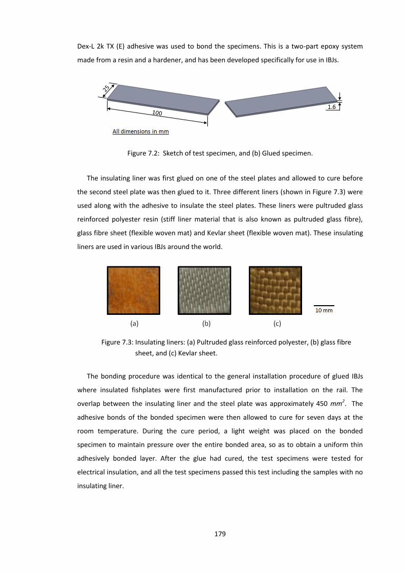
179

Dex-L 2k TX (E) adhesive was used to bond the specimens. This is a two-part epoxy system

made from a resin and a hardener, and has been developed specifically for use in IBJs.

Figure 7.2: Sketch of test specimen, and (b) Glued specimen.

The insulating liner was first glued on one of the steel plates and allowed to cure before

the second steel plate was then glued to it. Three different liners (shown in Figure 7.3) were

used along with the adhesive to insulate the steel plates. These liners were pultruded glass

reinforced polyester resin (stiff liner material that is also known as pultruded glass fibre),

glass fibre sheet (flexible woven mat) and Kevlar sheet (flexible woven mat). These insulating

liners are used in various IBJs around the world.

Figure 7.3: Insulating liners: (a) Pultruded glass reinforced polyester, (b) glass fibre

sheet, and (c) Kevlar sheet.

The bonding procedure was identical to the general installation procedure of glued IBJs

where insulated fishplates were first manufactured prior to installation on the rail. The

overlap between the insulating liner and the steel plate was approximately 450 mm2. The

adhesive bonds of the bonded specimen were then allowed to cure for seven days at the

room temperature. During the cure period, a light weight was placed on the bonded

specimen to maintain pressure over the entire bonded area, so as to obtain a uniform thin

adhesively bonded layer. After the glue had cured, the test specimens were tested for

electrical insulation, and all the test specimens passed this test including the samples with no

insulating liner.

180

7.2.2 Instrumentation of specimens

The transducer used in this study was the same as the one discussed and used in chapter

6. It was made from low cost, off the shelf piezoelectric discs formed from high sensitivity

lead zirconate titanate (PZT). As stated earlier in Chapter 6, the spatial resolution of the

measurements depends partly on the geometry of the sensor. Therefore, the disc elements

were cut down to form 6 mm 2 mm active area transducers in order to maximise the

resolution of the transducer to provide a narrow sensing area (Figure 7.4). When these were

excited, they emitted a gradually diverging ultrasonic sound wave approximately equal to the

dimensions of the sensor’s active area.

Figure 7.4: layout of sensor on a specimen.

Attenuation of ultrasonic signals in the adhesive layer is typically very high because of its

acoustic properties. Transmission of ultrasonic signal to and fro through the layer could

weaken the signal to extend that some important information might be lost. Therefore, in

order to obtain both qualitative and quantitative information from both the metal-adhesive

interfaces during the test, one piezoelectric sensor was permanently bonded directly to each

of the two surfaces of the epoxy adhesive glued specimen at the glued region using M-bond

200 (Vishay) adhesive. As shown in Figure 7.4, they were positioned on the opposite sides of

the centre line and 2 mm off the centre line of the specimen so that signals from one would

not interfere with the signals from another.

M-bond 200 (Vishay) adhesive was used because of its good adhesive strength and low

viscosity, and that it cures at room temperature. This was advantageous as the glued joint

cannot be placed in a high temperature oven to cure the adhesive. When the adhesive was

applied and the sensors were placed into position, sufficient pressure was then applied to the

sensors through a silicon rubber. The pressure on the sensors was continuously maintained

for 2 minutes while the adhesive sets. This is then left for 1 hour to allow for proper curing of

the adhesive. Once the sensors have been bonded to the specimen, coaxial cable was then

wired directly to the terminals of the transducer. The bonded sensors along with soldered

coaxial cable were then covered with epoxy resin at the points where they were soldered.

181

This helped to suppress transducer ‘ringing’ (back echo) and also to provide protection from

damage during handling. Figure 7.5 (a) shows the bonded transducers on the specimen, while

Figure 7.5 (b) shows a finish instrumented insulated adhesive joint specimen with coaxial

cable and epoxy cover.

Figure 7.5: (a) Bonded transducers on the specimen, and (b) Instrumented specimen.

7.2.3 Test Procedure for the tensile lap-shear test

Once the test samples had been produced and instrumented, shims were then attached to

the end of the steel sample as shown in Figure 7.6. This was to allow the load to act in line

with the bonded joint when the tensile load was applied and the joints were tested in pure

shear.

Figure 7.6: (a) Diagram of the of the test specimen.

The tensile lap-shear test was carried out on a Tinius Olsen Tensometer. A tensile force

was applied to shear the specimen at the glued joint while at the same time the change in the

contact condition of the joint was continuously monitored through the reading of the

ultrasonic reflection from the contact interfaces. The glued specimen was first assembled on

the tensometer as shown in Figure 7.7. The two transducers on the specimen were then

connected to the ultrasonic pulsing unit. Tensile force was introduced to the shear test

specimens by operating the tensometer under a constant displacement control, and the

specimens were gradually pulled apart (i.e., shear of the glued joints) at a constant rate of 1

mm/min.

(a)

(b)

10 mm

10 mm

182

Figure 7.7: Experimental setup on tensometer.

Ultrasonic monitoring was performed with each of the transducers excited with a 25 V

‘top-hat’ signal of 100 ns duration, with a pulser repetition rate of the ultrasonic set at 1 K

pulses per second. For each of the transducers, the delay time and range were configured to

cover the first four distinguished echoes of the ultrasonic reflection from the plate and the

glue interface in a time-domain window. The reflected signals were digitised by a digitizer on

the PC at a rate of 100 million samples per second, recorded and streamed directly to the

hard disk for storage. Prior to each test, a reference measurement of each of the sensors was

recorded while the insulated joint was still intact. The ultrasonic data of the test along with

that of the reference stored on the PC were post-processed to determine changes in the

ultrasonic reflection coefficient at the interface as the shear failure occurs.

7.2.4 Results

The dynamic reflection coefficient of the reflected ultrasonic signals from the interfaces

for each of the tests was calculated by dividing the reflected signal during the shear test by

the reference signal. The reflection coefficient gives a measurement of relative contact at the

interface as shearing of the insulated joint occurs. As mentioned in Chapter 3, an inverse

relationship exists between the reflection coefficient and nominal contact pressure. Thus, as

the value of reflection coefficient increases, the magnitude of contact pressure at the

interface decreases. The reference reading was taken when the bond was intact at the

beginning of the test. Therefore, when the value of reflection coefficient is 1, it indicates that

there is contact between the plate and the adhesive, and the bond between the adhesive and

the plate is still intact as per the initial state before the test. But as this value increases from

its initial value of 1, it implies that the contact between the interface of the plate and the

adhesive in decreasing and the plate is being separated from the adhesive as a failure (de-

bonding) occurs. This increment in the value of reflection coefficient continues until a

Test specimen Tensometer control system

183

constant value is reached when there is a separation of the surfaces. In the entire test, Sensor

1 measured the reflection coefficient of reflected signal at the interface between plate A and

the adhesive, while Sensor 2 measured the reflection coefficient of reflected signal at the

interface between plate B and the adhesive.

Figure 7.8: (a) A typical Ultrasonic reflection in time window with the gated waveform

used in calculation of RC marked using numeric labels (b) Measured reflection

coefficients from the reverberations of the reflected ultrasonic signal from the

adhesive-plate interface.

Figure 7.8 (b) shows a measurement of the dynamic reflection coefficient from a sensor in

a typical lap shear coupon test. As mentioned earlier, the delay time and range were set to

cover the first four reflected waveforms from the plate and the glue interface in a time-

domain window. The results of 1st WF to the 4th WF represent the calculated reflection

coefficient from each of the four reverberated waveforms of the reflected signal gated in a

time domain window as shown in Figure 7.8 (a). As can be seen, the same initial value of 1

was obtained from each of the waveforms, and this value increased sharply within a short

period to a maximum value as failure of the joint occurred at the interface. A constant

maximum value of 1.12, 1.42, 1.63 and 1.96 was obtained from each of the first four

waveforms respectively.

The reason for this observed increase in the value of the calculated reflection coefficient

from the waveforms can be explained by considering the schematic figure of the waveforms

of both the reflected and the reference signals shown in Figure 7.9. If the amplitude of the

first waveform of the reflected and the reference signals from the interface between the top

plate and the adhesive are respectively 0.9 and 0.8 of the pulse signals. And also, If successive

waveforms from a single point decayed by the same exponential factor of the amplitude of

the preceding waveforms, the amplitude of the 2nd, 3rd and 4th echoes of the reflected and

reference signals from the point will be 0.81, 0.73 and 0.66, and 0.60, 0.51 and 0.41

respectively. The calculated reflection coefficients for the four waveforms of the reflected

(a) (b)

1 2 3 4

(ns)

184

signal using the corresponding waveforms of the reference signal taken from a single point

will then be equal to 1.125, 1.266, 1.424 and 1.602 respectively.

Figure 7.9: (a) A typical Ultrasonic reflection in time window with the gated waveform

used.

In this present study, therefore, the reflection coefficient from the third reflected

waveform which gives a reasonably high value and can be clearly distinguished in all the tests

will be utilised in the presentation of the results of the monitored changes in the condition of

the contact interface during the tests.

The results of the tensile lap-shear tests are shown in Table 7.1. As it can be seen in all the

figures in the table, the load increases approximately at a constant rate from the value of

zero to a maximum value at which joint failed. The failure of the joints occurred rapidly

(ruptured) and after then, except in the case of Kevlar where there is a failure of the liner

material, the shear load decreases rapidly to zero and the failed joints supported no load.

This shows that the adhesive joints only performed elastically under shear load. In the case of

the failed joint with the Kelvar liner, the joint result shows that the joint sustained a fraction

of the peak shear load, and thus displayed a level of plastic behaviour after a majority of the

shear load has removed.

Adhesive

Top plate

Bottom plate

Time (s)

Reference Signal

Reflected Signal

0.90 0.80

0.81 0.64

0.73 0.51

0.66 0.41

185

Table 7.1: Results of the tensile lap-shear test of insulated adhesive joints.

B A

B A

B A

B A

B A

B A

B A

Dynamic reflection coefficient Failed joint specimen Liner type

Pultruded glass

fibre

Flexible glass fibre

Kevlar

(a)

(a)

(b)

(a)

(b)

(a)

(b)

Without Liner

(b)

A B

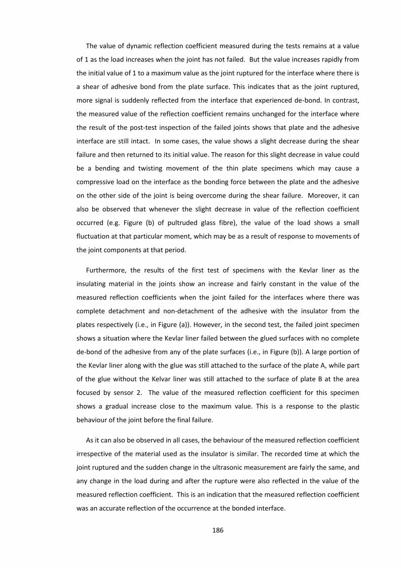
186

The value of dynamic reflection coefficient measured during the tests remains at a value

of 1 as the load increases when the joint has not failed. But the value increases rapidly from

the initial value of 1 to a maximum value as the joint ruptured for the interface where there is

a shear of adhesive bond from the plate surface. This indicates that as the joint ruptured,

more signal is suddenly reflected from the interface that experienced de-bond. In contrast,

the measured value of the reflection coefficient remains unchanged for the interface where

the result of the post-test inspection of the failed joints shows that plate and the adhesive

interface are still intact. In some cases, the value shows a slight decrease during the shear

failure and then returned to its initial value. The reason for this slight decrease in value could

be a bending and twisting movement of the thin plate specimens which may cause a

compressive load on the interface as the bonding force between the plate and the adhesive

on the other side of the joint is being overcome during the shear failure. Moreover, it can

also be observed that whenever the slight decrease in value of the reflection coefficient

occurred (e.g. Figure (b) of pultruded glass fibre), the value of the load shows a small

fluctuation at that particular moment, which may be as a result of response to movements of

the joint components at that period.

Furthermore, the results of the first test of specimens with the Kevlar liner as the

insulating material in the joints show an increase and fairly constant in the value of the

measured reflection coefficients when the joint failed for the interfaces where there was

complete detachment and non-detachment of the adhesive with the insulator from the

plates respectively (i.e., in Figure (a)). However, in the second test, the failed joint specimen

shows a situation where the Kevlar liner failed between the glued surfaces with no complete

de-bond of the adhesive from any of the plate surfaces (i.e., in Figure (b)). A large portion of

the Kevlar liner along with the glue was still attached to the surface of the plate A, while part

of the glue without the Kelvar liner was still attached to the surface of plate B at the area

focused by sensor 2. The value of the measured reflection coefficient for this specimen

shows a gradual increase close to the maximum value. This is a response to the plastic

behaviour of the joint before the final failure.

As it can also be observed in all cases, the behaviour of the measured reflection coefficient

irrespective of the material used as the insulator is similar. The recorded time at which the

joint ruptured and the sudden change in the ultrasonic measurement are fairly the same, and

any change in the load during and after the rupture were also reflected in the value of the

measured reflection coefficient. This is an indication that the measured reflection coefficient

was an accurate reflection of the occurrence at the bonded interface.

187

7.2.5 Discussion

In all the cases where it was observed that there was clear de-bond of the adhesive from

the surface of the plate during the failure of the joint, the value of the measured reflection

coefficient increases. This shows that as the failure of the joint occurs signal is increasingly

reflected from the interface of the plate as the epoxy adhesive shears away from the surface

of the plate. Whereas in case where the bond between the epoxy adhesive and the surface

of the plate remains intact after the failure of the joint, the value of the measured reflection

coefficient briefly showed a slight decrease during the period of the shear failure before

returning back to its original value of 1. In most cases, this change in value is negligibly small.

The reason for this can be attributed to changes in the stiffness of the adhesive layer as a

result of compression at the interface from the movement of the plates during the test. A

twisting movement of the plate would result in compression, and this was investigated by

carrying out a compression test on a metal-adhesive interface.

Figure 7.10: Schematic diagram of the experimental setup of compressive

loaded adhesive-steel plate interface.

Figure 7.10 shows a setup of a compression test on the steel-adhesive glued interface.

This involves loading of adhesive joint under a compressive load while single-point reflections

of the contact interface were recorded for a series of the loads. As shown in the diagram, a 4

mm layer of the Edilon Dex-L 2k tx (E) adhesive was cast and cured onto 15 mm diameter

upper steel specimen. A longitudinal wave ultrasound from a 10 MHz focused transducer

(this same transducer used in the static scanning of bolted joint in chapter 4) was coupled

and focused on the glued interface of the adhesive and the upper specimen using a water

bath assembly. The specimen was then loaded incrementally in compression using a hydraulic

loading jack. At each of the load increments, the reflected signal separated in a time domain

188

from the interface was recorded and store on the PC for analysis. A reference measurement

was also recorded prior to the loading of the specimen.

Figure 7.11: Measured reflection coefficient for a series of loads on the metal-adhesive

interface.

It can be seen from the results of the test shown in Figure 7.11 that as the contact

pressure increase from 0 MPa to an approximately value of 2 MPa, the value of the measured

reflection coefficient dropped substantially to a value of 0.904. A further increase in the

contact pressure only led to a very small change in the value of the reflection coefficient. An

approximately value of 0.82 was recorded at the contact pressure of 12 MPa, which is a

difference of 0.08. The drop in the reflection coefficient can be attributed to changes in the

stiffness of the adhesive caused by the compression of the layer, assuming a negligible

change occurs in the steel [108]. During the rupture process, a reasonable pressure is

expected to occur. Hence, increase in stress will cause the stiffness of the glue layer to

increase, which will result in an increase in the acoustic impedance of the layer.

189

7.3 Shear Test of Insulated Block Joint

In the previous sections of this chapter, an experimental shear test was conducted on lap

joints with different insulating materials commonly used in the construction of insulated block

joints in the rail industries, and the response of ultrasound at the interface of these joints to

shear load has been observed. The next phase of this study will be committed to experimental

shear test on insulated block joints with different insulating liners between the fish plate and

the rail. This is to gain an appreciable understanding of the performance of ultrasound on the

glued insulated block joints with different liner materials that constitute the interface

between the fishplates and the rail.

The insulated joint specimens used in this study consisted of rail, fishplates and insulated

liners. The joint was constructed with the glued insulated liners between the rail and the

fishplates, and then sectioned into 50 mm widths as shown in Figure 7.12. Three different

liners (pultruded glass fibre liner, glass fibre sheet and Kevlar sheet) were used as insulating

material in the rail joints. A slot was cut on the top of the rail head parallel to the upper

fishing surface where the fishplate comes in contact with the rail head. Another slot was cut

at the foot of the rail parallel to the lower fishing surface. A 10 mm 30 mm slotted hole was

drilled in the centre of the web of the rail to a depth of 25 mm. These slots were cut, as shown

in Figure 7.12, parallel to the contact interfaces between the surface of the rail head at the

top and the top of the fishplate, the rail web and the face of the fishplate and, the foot of the

rail and the bottom of the fishplate. This is to allow the respective interfaces to be monitored

by normal incidence longitudinal ultrasonic signals which will travel perpendicular to the

corresponding interfaces and the cut surfaces.

Figure 7.12: (a) Image of a rail showing terminology (b) IBJ with slots at the top of the

rail head, the bottom of the rail foot and the middle of the rail web.

190

The construction of the joint specimens (i.e. the gluing, the cutting of slots and the

sectioning of the insulated block joint specimens) were done at LBFoster Rail Technologies’

site in Sheffield, United Kingdom. Four IBJ specimens were produced, and were named:

LBFC1, LBFC2, LBFC3 and LBFC4 having pultruded glass reinforced polyester resin, Kevlar

sheet, Kevlar and flexible glass fibre sheet sheet as insulated liner material respectively.

7.3.1 Instrumentation of the insulated block joint specimens

The low cost, off the shelf piezoelectric discs formed from high sensitivity lead zirconate

titanate (PZT) were also used as the transducer sensor in this experimental study. In order to

cover and monitor a reasonable portion of the contact area in the areas of interest,

unmodified disc’s size was used. Six piezoelectric sensors were permanently bonded to each

of the test specimens. As shown in Figure 7.13, one sensor was bonded to the centre of each

of the cut surfaces, one sensor was bonded to each of the sides of the slotted rectangular

hole and one sensor was bonded to each side of the fishplates with M-bond 200 (Vishay)

adhesive. The surface of each of the fishplates was ground to reduce the surface roughness

so that the sensor can be well bonded to the surface. This is to ensure good acoustic coupling

that will allow sufficient ultrasonic energy to pass into the specimen.

The sensors were bonded to the specimen using the same procedure described in section

7.3.2. Once the sensors had been bonded to the specimen, a coaxial cable was then wired

directly to the terminals of the sensors. The bonded sensors along with soldered coaxial

cables were then covered with epoxy resin at the points where they were soldered. Figure

7.14 shows an instrumented IBJ specimen. As can be noted in the figure, the cuts on the top

and at the foot of the rail were done on one side of the specimen as it was expected that

identical responses to shear loading would be recorded from both sides. Therefore,

monitoring the response of the bonded fishing interfaces between the fishplate and the rail

from a one side will save time and cost of production of the specimens.

191

Figure 7.13: Bonded transducers on the specimen.

Figure 7.14: (a) Instrumented IBJ specimen (b) Schematic diagram of instrumented IBJ

showing the anticipated paths of ultrasonic signals.

7.3.2 Shear test of the IBJs

The instrumented IBJ was positioned, as shown in Figure 7.15, on a plate that has two

raised sections made from a fishplate that sat underneath the fishplate cross sections of the

sectioned IBJ. A section of rail was then placed on the sectioned IBJ such that the two rail

profiles align. The transducers on the IBJ specimen were then connected to the ultrasonic PC.

192

Figure 7.15: Experimental setup of the IBJ.

The shear test of the joint specimens was carried out on a hydraulic compression test rig

(as shown in a picture of the test setup in Figure 7.16). During the test, the IBJ specimen and

the setup were made parallel with each other to ensure both sides of the test sample are

loaded evenly. The joint specimen was loaded vertically, while sitting horizontally, at a

constant displacement rate through the rail section until the fishplates were sheared away

from the rail. Furthermore, the loads exerted on the joint were recorded with the

corresponding time and the displacement.

Figure 7.16: Experimental setup of the IBJ on the displacement controlled hydraulic machine.

193

During the test, ultrasonic monitoring of the contact interfaces of the joints was

performed with each of the transducers excited with a 25 V ‘top-hat’ signal of 100 ns duration

with a pulser repetition rate of the ultrasonic set at 1 kHz. For each of the six transducers, the

delay time was set to capture the reflected signals from the interface of interest, and the

reflected signal waves were isolated in a time domain window of 1200 ns. The reflected

signals from all the sensors were then digitised, recorded and streamed directly to the hard

disk of the PC. Prior to the test, a reference measurement for each of the sensors was

recorded while the insulated block joint was still intact. The stored ultrasonic data on the PC

were later post-processed to determine changes in the reflection of the ultrasonic signals

from the interfaces as shear occurs.

7.3.3 Results

The schematic diagram of the IBJ shown in Figure 7.17 indicates the points at the

interfaces where the reflection coefficients were measured. Fishplate 1 and Fishplate 2 are

the reflection coefficients measured at the interface between the insulator and the fishplates

by sensor 1 and sensor 2 respectively as specified in Figure 7.14 (b) in section 7.2.1, while

Web side 1 and Web side 2 are the reflection coefficients measured at the interface between

the insulator and the sides of the rail web by sensor 3 and sensor 4 respectively. In addition,

the Top is the reflection coefficient measured at the interface between the insulator and the

upper fishing surface of the rail head by sensor 5, and the Foot is the reflection coefficient

measured at the interface between the insulator and the lower fishing surface of the rail foot

by sensor 6.

Figure 7.17: Schematic diagram of instrumented IBJ with the represented names of the

interfaces.

194

It can be observed from Figure 7.17 that the top and bottom slots were made only on one

side of the rail. This was to allow simultaneous monitoring of the three interfaces between

the fishplate and the rail from the same side, and consequently, easy evaluation of their

response to loading from the same load point. The cut of the slots on only one side equally

reduces cost of production of the joint since similar responses are expected from both sides

of the rail as the features on both are the same.

Table 7.2: Visual observation of test specimens with pultruded glass fibre and flexible

glass fibre sheet as insulator after the shear test.

Point of Reflection

Visual Observation

LBFC1: Pultruded glass fibre

Top Clear de-bond of the glue with the insulator from the surface

Fishplate 1 No de-bond of glue with the liner from the surface

Fishplate 2 No de-bond of glue with the liner from the surface

Foot No clear de-bond of the glue with the insulator from the surface, but partial tear out of liner from the glue

Web side 1 De-bond of the glue with the insulator from the surface with a tiny residue of glue at some part where the sensor focused

Web side 2 Clean de-bond of the glue with the insulator from the surface

LBFC4: Flexible glass fibre sheet

Top No de-bond of glue from the surface, but the liner roughly

torn away in some place from the glue.

Fishplate 1 No de-bond of glue with the liner from the surface

Fishplate 2 No de-bond of glue with the liner from the surface

Foot Partial de-bond of the glue with the insulator from the surface

Web side 1 Clear de-bond of the glue with the insulator from the surface

Web side 2 Clear de-bond of the glue with the insulator from the surface

at the part where the sensor focused

The results of the post-test visual inspection of the test specimens were presented in

Tables 7.2 and 7.3, and the results of the shear test of the insulated block joints are shown in

195

the Figures 7.18 and 7.19. Each of the test figures show the measured applied shear load as

well as the measured reflection coefficients from the six above-mentioned interfaces during

the test. The value of the measured applied shear load increases from 0 at the

commencement of the test to a maximum as the machine exerts a displacement at a

constant rate on the joint until the fishplates were sheared away, and the value of the

applied shear load rapidly returned back to zero. During this period, the values of some of the

measured reflection coefficients of the reflected ultrasonic signals from the six interfaces,

calculated by dividing the respective reflected signal during the shearing test by their

reference signal, increases from the initial value of 1 to a maximum value as the joint

sheared. However, the value of the measured reflection coefficient of some of the interfaces

shows a slight decrease.

Figure 7.18: Measured reflection coefficients and shear load during the shearing test

of IBJs with pultruded glass fibre and flexible glass fibre sheet.

7.3.3.1 IBJ with pultruded glass fibre liner and IBJ with flexible glass

fibre liner

The results of the shear test of IBJ with pultruded glass fibre as the insulator between the

joint interfaces are shown in the LBFC1 of the Figure 7.18. As it can be seen in the figure, the

fairly linear increase in the value of the measured shear load to a maximum value and the

196

sudden decrease to a value of 0 shows that the joint only performed elastically and after the

failure, could not display any plastic behaviour. During this period of the elastic behaviour of

the joint, the value of the measured reflection coefficients remains constant at an

approximate value of 1 until 90% of the total applied load on the joint had been expended

before a small but gradual increase in value. This increment was for a short period until 97%

of the peak applied shear load on the joint was reached.

The value of the reflection coefficient experienced a sudden and fairly linear increase in

value to a constant maximum value during the remaining 3% of the peak applied shear load.

After the rupture of the joint, the value of the reflection coefficient remains constant which

indicates that there was no further interaction at the interface as the joint could not sustain

any plastic failure. Furthermore, the results also show that there was an increase in the value

of the measured reflection coefficients from only the sensors where there were clear de-

bonds after the rupture of the joint. Measured values from the remaining sensors where

there were no bonds remain approximately constant at 1.

The response of the IBJ with flexible glass fibre as the insulators (LBFC4) to shear load

shows a similar feature to that of IBJ with pultruded glass fibre (LBFC1), except that it

sustained insignificant amount shear load after the rupture of the joint when more than 95%

of the peak shear load had been removed. This might be due to the joint movement at the

instance and more importantly, the shearing of the liner material itself. The measured

reflection coefficients from the sensors that monitored the rail web during the test increase

to their maximum values shortly after the commencement of the loading. This was when the

applied shear load was only approximately 20 % of the peak load that ruptured the joints. In

contrast, the measured reflection coefficient from the foot reached the maximum value as

the joint ruptured. Furthermore, post-test inspection of the test specimen after the test

(Table 7.2) shows that there was partial de-bond of adhesive glue from the surface web side

1. This is likely the reason for the small change in the value of the measured reflection

coefficient compare to that of web side 2 where a complete de-bond of the glue was

observed.

7.3.3.2 IBJ with Kevlar liner

The results of the shear test on the IBJ with Kevlar liner as the insulator (LBFC3 and LBFC5)

are shown in Figure 7.19. The results of the post-test inspection of the failed joints are

presented in Table 7.3. The results in the figure show that the joint behaves elastically during

the loading to peak value before the sudden failure. The joint also shows some plastic

197

behaviour by supporting some loads after the peak applied load is reached, and the majority

(approximately 75%) of this peak shear load had been removed. Whenever there are clear

de-bonds, according to the results of the post-test inspection, the values of most of the

measured reflection coefficients experienced increment right from the onset of the increase

in the loading of the joints. While the maximum value of some of these reflection coefficients

was attained within a short period during the loading of the joint, the increment continues

until the failure of the joints. As it can also be observed in the figure, there is a period of small

but gradual increase in the value of the reflection coefficients just before the maximum

values is attained, and this represents the period at which the joint displayed plastic

behaviour before total failure.

Table 7.3: Visual observation of test specimens with Kevlar sheet as insulator after the

shear test

Point of Reflection

Visual Observation

LBFC2: Kevlar sheet

Top Clean de-bond of the glue with the insulator from the surface

Fishplate 1 No de-bond of glue with the liner from the surface

Fishplate 2 No de-bond of glue with the liner from the surface

Foot Clean de-bond of the glue with the insulator from the surface

Web side 1 Partial de-bond of the glue with the insulator from the surface

Web side 2 Clean de-bond of the glue with the insulator from the surface

LBFC3: Kevlar sheet

Top No de-bond of glue from the surface, but the liner detached

from the glue.

Fishplate 1 No de-bond of glue with the liner from the surface

Fishplate 2 No de-bond of glue with the liner from the surface

Foot Clean de-bond of the glue with the insulator from the surface

Web side 1 De-bond of the glue with the insulator from the surface, but a

residue of glue remains on the surface

Web side 2 Clean de-bond of the glue with the insulator from the surface

198

Figure 7.19: Measured reflection coefficients and shear load during the shearing test

of IBJs with Kevlar liner.

7.3.4 Discussion

The response of the joints to shear loading before the sudden failure are similar, as they

all exhibit elastic behaviour. Immediately after the failure (rupture), they were unable to

sustain any load and thereby displaying no plastic behaviour. Except the joint made with

Kevlar as the insulator that performed plastically after more than 75% of the peak shear load

had been removed. Joint made with flexible glass fibre also sustained an insignificant amount

of the shear load more than 90% of the peak shear load had been expended. Unlike the

smooth surface pultruded glass fibre, the other two insulating liners were made of woven

materials that allow the adhesive glue to impregnate the weave fabric. This gives a better

resistance to clean shear during the failure at the interfaces. Moreover, the woven material

of the flexible glass fibre has a smoother surface than the weave fabric of the Kevlar liner,

hence sustained less of the peak shear load after failure. Just as also seen in the test of the

lap joints, the partial de-bonding and failure of the Kevlar liner itself responsible for this

characteristic behaviour. This is advantageous in a safety critical situation where the failure

can be noticed and repaired before final failure.

It can be observed from the results of the shear tests of the IBJs that there is an

agreement between the measured reflection coefficients and the post-test inspection of the

199

sheared IBJs. The features shown in the results of the test of the lap joints can also be

identified in the results of the insulated block joints. The results indicate that wherever there

was de-bond of the glue from the surface of the rail during the failure of the joint, the value

of the measured reflection coefficient increases. As stated earlier in section 7.1.4, this was

due to more signals being reflected from the interface where the glue sheared away. It was

also observed that there was a negligible small decrease in the value of reflection coefficients

of some interfaces that remain intact during the test. This also has been attributed (as

explained in section 7.1.5) to compression load on the glue layer caused by the twisting of the

IBJ components as shear occurs. It led to a momentary increase in the stiffness of the

adhesive and resulted in an increase in the acoustic impedance of the glue layer. The values

usually returned to their initial value of approximately 1 after the shear failure of the joints.

The negligible small decrease in the value of reflection coefficients is more pronounced in

the results of the joints with Kevlar liner than in the joints with the other two insulating

materials. This is due to the same reasons given for the plastic behaviour of the joints after

failure. The joints with Kevlar liner sustained more plastic response than the other two

insulating materials due to better resistance to a clean shear at interface and hence, produce

more twisting movement of components during the failure of the joints. Furthermore, the

protruded insulating liner gives little resistance to a clear shear compared to Kevlar and

flexible glass fibre insulating liners. Therefore, the values of the reflection coefficient

experienced a sudden rise to a maximum value at the rupture of the joint. Whereas, the

results of the tests of the IBJs with the Kevlar as insulator (with more resistance to a clean

shear at the interface) show a gradual increase in the values of the reflection coefficient

before attaining the constant values. The increase in the value of the reflection coefficient

commenced earlier when compared to the joints with protruded insulating liner.

The results of the measured reflection coefficient from the fishplate 1 and fishplate 2

(interface between the fishplates and the adhesive glue with the insulators) revealed that, in

all cases, the values of the reflection coefficient remain approximately unchanged during the

test. The results of the post-test inspection carried out on the sheared IBJs also revealed that

these interfaces remain intact during the tests. However, the results of the measured

reflection coefficient and the post-test inspection show that, in all cases, de-bond occurred at

the interface of the head of the rail (upper fishing) and the insulator, and at the foot of the

rail (lower fishing) and the insulator. It also occurred at the interface adjacent to the web.

The de-bonding of adhesive/insulating layer on the web sites is observed to occur earlier

than at any other parts of joint in most of the tests. The results of the ultrasound monitoring

200

always indicate that de-bonding had taken place when the applied load was only some

fractions of the peak shear load. Whereas, the de-bonding at the top and foot of the rail

occurred almost at the peak of the shear load. These observations are in agreement with the

studies conducted by Peltier and Barkan [143] where it was observed that epoxy de-bonding

begins and remain extensive at the endpost. It then extends to the to the insulator layer

adjacent to the web where it widely propagates further.

Lastly, the observed agreement that exists between the results of the shear load, the post-

test inspection and the results of the ultrasonic monitoring of the insulated joints shows that

ultrasound can be a potential tool for the monitoring of IBJs in the rail industry.

7.4 Conclusions

A non-intrusive technique has been used to monitor de-bonding at the interface of

adhesive bonded insulated lap joints and insulated block joints, subjected to shear load

induced failure. The technique utilised the reflection of the normal incidence longitudinal

ultrasonic signals from the adhesive interface to monitor the contact condition at the

interface. The results of the tests show that whenever there is de-bond of the adhesive glue

at the interface during the failure of the joints, the value of the measured reflection

coefficient typically increases. It was also observed that there was a negligibly small decrease

in the value of reflection coefficients of some interfaces that remain intact during the test. It

was attributed to a compression load on the adhesive layer caused by the twisting of the joint

components as shear occurs. The small decrease in the value of reflection coefficients is more

pronounced in the results of the joints with Kevlar liner as an insulator.

Also, the results of the measured reflection coefficient show that all the joint exhibit

elastic behaviour before the failure of the joints. Only joints made with a Kevlar liner as the

insulator displayed a pronounced plastic behaviours after the rupture of the joints by

retaining a fraction of the shear load before final failure of the joint. This is advantageous for

a safety critical condition.

The results of the tests show that de-bond occurred at the interface of the head of the rail

(upper fishing) and the insulator, and the foot of the rail (upper fishing). Also, de-bond

occurred at the insulator and at the interface adjacent to the web. While the failure of the

adhesive bond on the web is observed to occur earlier than at any other parts of the IBJs

when the applied load was only some fractions of the peak shear load, the de-bonding at the

201

top and foot (upper and lower fishings) of the rail occurred almost at the peak of the shear

load. Furthermore, the values of the reflection coefficient experienced a sudden rise to a

maximum value at the rupture in the joint with protruded glass liner. Whereas, the results of

the tests of the IBJs with the Kevlar as an insulating liner (with more resistance to a clear

shear at the interface) show a gradual increase in the values of the reflection coefficient

before attaining the constant values during shear test.

Finally, adhesive bonding of structural components is commonplace in the aerospace and

automotive industries where substantial experience has been built up for the testing of

products during the manufacturing process. Moreover, previous studies have been focused

on adhesive joints where the adhesive is the only material between the bonded components.

However, the present study has applied an ultrasonic technique to investigate adhesive joints

that have insulating materials bonded between the bonded components and subjected to

shear induced failure. The results have shown a potential that the technique can be used as a

tool to monitor failure of IBJs in the railway industry. Therefore, the knowledge gained in this

chapter will be taken forward to conduct a conditioning monitoring test of full insulated block

joints in the next chapter.

202

Chapter 8 Application of Ultrasound for Condition Monitoring of Insulated block joints

Application of Ultrasound for Condition Monitoring of Insulated Block Joints

8. Despite a number of the known disadvantages associated with mechanical rail

joints, they are considered a necessary component on rail tracks. They are

installed at regular intervals in rail tracks to connect strings of continuous

welded rail together for engineering and economic reasons. The joints are

substantially weaker than the rail and are subjected to large stresses, causing

failure, which can be disruptive to railroad operations and may lead to the risk

of a train derailment that in some cases is of fatal consequences. In the previous

chapters, studies have been conducted on both static and dynamic bolted joints

under static and dynamic loads, and also on insulated adhesive lap joints and

sectioned insulated block joints under shear load. In the present chapter, studies

shall be carried out on a full scale insulated block joints under dynamic shear

load. Bring together all knowledge gained in the preceding works, investigations

will be conducted on the response of the insulated adhesive interface of IBJs to

failure induced loading. A non-invasive ultrasonic technique will be used with

the objective to understand and monitor the adhesive de-bonding in IBJs, and

also the relaxation of contact interface in these joints. This will assist to

establish a technique of monitoring rail joints in service.

8.1 Introduction

One of the essential components of the railway is the rail joints which are primarily bolted

joints that connect pieces of rails together. The mechanical connectors consist of fishplates

and fasteners (bolts and nuts) that mount the fishplates to the web sides of the rail, as shown

in Figure 8.1 of a glued insulated block joint. The mechanical rail joints, especially the IBJs, are

often required at every few kilometres along railway tracks, where they introduce weak

points in the track. Therefore, causing high maintenance schedules and service disruptions

that cost the railway industry vast amounts of money.

203

Figure 8.1: Glue insulated block joint [171].

Most of the research works on rail joints have been focused on improving their service

lives using finite element methods to investigate the stresses and strain development around

rail joints. Many of the experimental studies conducted on rail joints investigate the fatigue

life of joint bars, stress concentrations in the rails and fishplates caused by bolt holes, stresses

due to head contact and head-free joint bars. Many of the problems associated with IBJs

started with the deterioration in the adhesive interface that holds the joint together [5]. The

debonding of the adhesive in an IBJ is progressive in nature and, if unattended, will eventually

convert the IBJ to the regular conductive rail joint with poor integrity [143].

As mentioned in chapter two under the literature review, some authors have used Strain-

gauge-based technique [143] to measure changes in the tensile strain in IBJs in response to

longitudinal load over time, with the believe that the strain distribution within the joint

changes when there is loss of epoxy bonding in the IBJs. The laboratory reading of the

changes in the strain measured by smart strain gauges attached to the side of the fishplate of

a rail joint subjected to tensile load was correlated to the result from finite element methods

to measure longitudinal movement in the IBJ. This was used to evaluate de-bonding in the

joint. However, the assumption that the response of joints to dynamic loads from the rail

vehicle and impact factor which varies daily due to uncontrolled and unmeasured variables

such as modulus of the support of the railroad track will not affect the reading from the

device are issues. Also, the accuracy of such device is also at the mercy of average daily

variation in the environmental temperature.

As mentioned earlier, IBJs failure causes substantial disruption to railroad operation, and

maintenance of them in railway tracks cost huge amounts of money. Visual inspection

techniques, presently employed to detect defects in insulated block joints are labour

intensive and prone to human errors. Moreover, this method cannot reveal any de-bonding

of epoxy at the clamped interface between the fishplate and the web sides of the rail. Since

many of the problems in IBJs start with the deterioration in the epoxy that holds the joint

together, timely and reliable information, with a minimal human intervention, about the

conditions of the joints will be beneficial. This will not only allow for an enhanced

204

replacement plan before a complete failure occurs, but will improve the overall maintenance

regime of IBJs. Therefore, using the knowledge gained in the previous chapters, the present

study intends to investigate the change in contact conditions at the glued interface of a full-

scale IBJ under the dynamic shear loading. A non-invasive ultrasonic technique will be used in

this study, with an aim to establish a practical condition monitoring technique for insulated

block joints, which is independent of the loading situations and variable conditions at the

point of installation.

The author will like to state here that this particular study was carried out together with

Philip Beaty [127]. The aspect of the author was mainly focused on the ultrasonic monitoring

of the deterioration and failure of the bonded interface of the IBJs during the dynamic shear

loading, with the aim to establish a practical condition monitoring technique for such joints.

While Philip Beaty aim was to compare the performance of two IBJs designs whilst assessing

the life cycles of the joints using the loading technique employed in this chapter. Therefore,

aims and presentation of reports were different.

8.2 Experimental Procedure

Stresses in IBJ are quite complex, tensile stresses in an IBJ can result in the shear stress in

the epoxy layer, while bending of the rail and the joint can produce additional stresses in the

adhesive. In order to understand the response of ultrasonic signals to the change in contact

condition of the glued insulating surfaces of IBJ, a tensile lap-shear test was first conducted

on glued insulated lap joints, followed by the experimental shear test of insulated block joints

with different insulating liners in Chapter 7. The last phase of the study, which involves the

experimental shear test of full insulated block joints under dynamic loading, was done using

the same procedure highlighted in Chapter 7. The ultrasonic equipment (FMS100 System)

used in the previous experiments was also utilised. Figure 8.2 shows the schematic diagram

of the ultrasonic unit and a sectioned view of the instrumented IBJ specimen.

Figure 8.2: Schematic diagram of the ultrasonic equipment and a section of an IBJ.

205

8.2.1 Test specimen

The IBJ specimen used in this study is a 4-bolt adhesive glued insulated block joint. The IBJ

is used to join two 3 m EN13674-56E1 flat bottom rails together (Figure 8.3). The construction

of the insulated block joint specimens was done at LBFoster Rail Technologies’ site in

Sheffield, United Kingdom. Two full-scale IBJ specimens were produced and were named:

LBFR1 and LBFR2 having pultruded glass reinforced polyester resin and flexible glass fibre

sheet as the insulating material in the joints respectively. Apart from the material difference

in the insulating liner, the fishplates manufacturing process was different, as they were

created in different moulds. The LBFR1 fishplates were cast in a relatively loose mould, and

their shape is determined primarily by the fishplate and the insulating liner themselves. The

LBFR2 fishplates were made in a mould that is made from a piece of rail, and because the

liner is flexible the shape of the fishplate is determined by the mould. The LBFR2 is a new

design with improved accuracy and smaller manufacturing tolerance over the LBFR1 which is

a standard joint currently use in the UK. The LBFR2 has a greater stiffness at higher loading

than the LBFR1 [127]. The IBJs used for the testing were four bolt design as these are weaker

than 6-bolt joints and hence, the joint failure would be accelerated. Furthermore, the joints

were fastened using the UK standard fastening system of 1.1/8” swage fasteners which give a

260 kN clamping force.

Figure 8.3: 4 bolted adhesive glued insulated joint specimen.

8.2.2 Instrumentation of the IBJ specimens

Unmodified piezoelectric discs formed from high sensitivity lead zirconate titanate (PZT)

are used as the transducer sensor in this experimental study. Eight piezoelectric sensors

were permanently bonded to each of the test specimens; four to each of the two fishplates.

As shown in Figure 8.4, the sensors were bonded closely to the fasteners (bolt and nut). This

is because the results of the previous works have shown that the closer the distance to the

206

bolt hole, the higher the contact pressure at the bolted interface. Sensors were bonded at a

distance of 20 mm and 200 mm on the each side of the endpost which was at the centre of

the joint with M-bond 200 (Vishay) adhesive.

The structure of the rail joints was left as-received as any modification that introduced cut

on them might initiate and accelerate fatigue failure of the specimen during the dynamic

shear loading. Moreover, the objective of this study is to study the failure of unmodified IBJ

with an aim of developing a technique for monitoring such IBJ in the service. Hence, the rail

joints used were not tampered with and their integrity was left in as-manufactured and as-

received states. The surface of each of the fishplates was only cleaned with abrasive paper

and acetone to remove dirt at the areas where the sensors were to be glued. This was

important in order to ensure good acoustic coupling that will allow sufficient ultrasonic

energy to pass into the specimen and back to the bonded sensor at the surface of the

fishplate.

Figure 8.4: Bonded transducers on the specimen.

The sensors were bonded to the specimen using the same procedure described in Section

7.2.1 in Chapter 7. Once the sensors had been bonded to the specimen, coaxial cable was

then wired directly to the terminals of the sensors. The bonded sensors along with soldered

coaxial cables were then covered with epoxy resin at the points where they were soldered.

This helps to suppress ringing (back echo) and also protect the sensor from damage during

handling of the IBJ specimen. Figure 8.5 shows the instrumented IBJ specimen.

Figure 8.5: Instrumented full IBJ specimen.

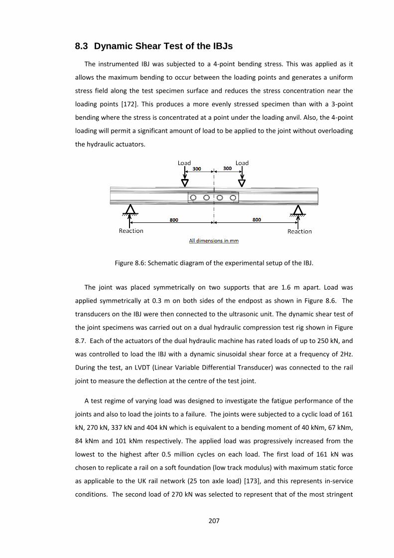
207

8.3 Dynamic Shear Test of the IBJs

The instrumented IBJ was subjected to a 4-point bending stress. This was applied as it

allows the maximum bending to occur between the loading points and generates a uniform

stress field along the test specimen surface and reduces the stress concentration near the

loading points [172]. This produces a more evenly stressed specimen than with a 3-point

bending where the stress is concentrated at a point under the loading anvil. Also, the 4-point

loading will permit a significant amount of load to be applied to the joint without overloading

the hydraulic actuators.

Figure 8.6: Schematic diagram of the experimental setup of the IBJ.

The joint was placed symmetrically on two supports that are 1.6 m apart. Load was

applied symmetrically at 0.3 m on both sides of the endpost as shown in Figure 8.6. The

transducers on the IBJ were then connected to the ultrasonic unit. The dynamic shear test of

the joint specimens was carried out on a dual hydraulic compression test rig shown in Figure

8.7. Each of the actuators of the dual hydraulic machine has rated loads of up to 250 kN, and

was controlled to load the IBJ with a dynamic sinusoidal shear force at a frequency of 2Hz.

During the test, an LVDT (Linear Variable Differential Transducer) was connected to the rail

joint to measure the deflection at the centre of the test joint.

A test regime of varying load was designed to investigate the fatigue performance of the

joints and also to load the joints to a failure. The joints were subjected to a cyclic load of 161

kN, 270 kN, 337 kN and 404 kN which is equivalent to a bending moment of 40 kNm, 67 kNm,

84 kNm and 101 kNm respectively. The applied load was progressively increased from the

lowest to the highest after 0.5 million cycles on each load. The first load of 161 kN was

chosen to replicate a rail on a soft foundation (low track modulus) with maximum static force

as applicable to the UK rail network (25 ton axle load) [173], and this represents in-service

conditions. The second load of 270 kN was selected to represent that of the most stringent

208

qualification test that could be found in a similar section of rail size [174]. The highest load

(404kN) represents a 2.5 factor of safety over the first load, and this was also close to the

operational limit of the test rig being used. The third bending moment was selected to be the

average of the second and the highest loads. The application of the third and the highest

loads was to accelerate the failure of the joint.

Furthermore, the ultrasound monitoring of the contact interfaces of the joints was

performed using a procedure similar to the shear of the IBJ in Chapter 7. The reflected signal

waves from the interface for each of the transducers on a rail joint were isolated in a time

domain window of 1200 ns. The reflected signals were then digitised, recorded and streamed

directly to the hard disk of the PC. Also, the reflected signals were recorded at two intervals

equally spaced daily, for the duration of the test. This was to reduce the amount of data

acquired and saved on the PC. The stored ultrasonic data were later post-processed to

determine changes in the reflection coefficient of signals from the interface during the test.

Prior to each test, a reference measurement of each of the sensors was recorded while the

insulated block joint was still intact. As the reference is not taken from unglued plane

fishplates, the reflection coefficient that will be measured is expected to start at 1 and rise.

This will be similar to the results of the shear test of the insulated adhesive joints in Chapter

7.

Figure 8.7: Experimental setup of the IBJ on the dual hydraulic loading rig.

209

8.4 Results

The dynamic loading test on the two IBJs resulted in fatigue failure of the joint specimen

with the pultruded glass reinforced polyester resin at the insulating layer (Figure 8.8) at

approximately 1.7 million loading cycles, and fatigue failure of the rail of the specimen with a

glass fibre sheet as the insulating material (Figure 8.13) at approximately 1.5 million loading

cycles. Table 8.1 shows the measured deflections at the centre of the joints with the

corresponding applied loads and calculated bending moments. Furthermore, the results of

the deflection and the corresponding measured reflection coefficient from the interface of

the IBJ during the test are shown in Figure 8.10. Sensor 4 on the LBFR1 IBJ got damaged

during the experimental set-up and, therefore, no measurement was recorded by this sensor.

Figure 8.8: Failed IBJ on the dual hydraulic loading rig and the failed LBFR1 IBJ.

As can be seen from the results of the LBFR1 IBJ (Table 8.1 and Figure 8.10), during the

first three consecutive applied loads (161 kN, 270 kN and 337 kN), the deflection remains

fairly constant throughout the loading cycles for each of the loads. This indicates that the

adhesive bond at the interface was still intact, and the stiffness of the joint was still elastic.

While a linear relation exists between the load and the average deflection at the centre of the

joint up to a load of 404 kN (Figure 8.9), and the calculated stiffness of the joint during this

period is 52.9 kNm-1. But at the load of 404 kN when the joint was cyclically loaded, the

deflection at the centre varies from being constant and started to show a plastic behaviour

until the joint failed by fatigue of the fishplates.

210

Table 8.1: Measured deflection at the centre of the IBJs

Cycles

(106)

LBFR1 IBJ LBFR2 IBJ

Load (kN) BM (kNm) Deflection (mm)

Deflection (mm)

161 40.0 0 2.23 2.60

0.1 2.31 2.31

0.2 2.25 2.31

0.3 2.26 2.30

0.4 2.29 2.33

0.5 2.31 2.35

270 67.4 0.5 3.94 4.37

0.6 3.83 4.13

0.7 3.85 4.15

0.8 3.87 4.16

0.9 3.93 4.17

1.0 3.86 4.23

337 84.2 1.0 4.98 5.38

1.1 5.18 5.36

1.2 5.21 5.36

1.3 5.23 5.40

1.4 5.24 5.37

1.5 5.24 5.38

404 101.0 1.5 6.32 7.05

1.6 7.74

1.7 7.92

Figure 8.9: Average deflection at the centre of IBJ and applied load.

211

Figure 8.10: Measured reflection coefficients and deflection at the centre of the IBJ

with protruded glass fibre.

The values of the measured reflection coefficient from all the sensors during the test show

a similar trend, and with changes occurred at the same time. This observation is as a result of

the fairly uniformly stress experienced by the joint situated between the points of the

application of load when subjected to four-point bending stress. Furthermore, during the

period of constant deflection of the joint (elastic behaviour), the values of the measured

reflection coefficient from the sensors show a fairly constant value except at the ½ million

cycles (onset of the 270 KN loading). While increase shows that more signals were reflected

due to separation of the interface, the sudden increase in value of the reflection coefficient is

a characteristic behaviour of adhesive bonded joints at failure as observed in Chapter 7 under

the shear test of adhesive joints. Therefore, the observed increase in value is an indication of

adhesive bond failure (rupture) at the interface of the fishplate and insulator. After this

point, the values return gradually to the initial values over a period of approximately 200,000

cycles. This shows that more signals were transmitted across the interface due to increase in

conformity at the interface. This can be attributed to the effect of the compressive force

from the bolted fasteners on the adhesive interface.

During the next 1 million cycles that witness the increase in applied load from 270 kN to

337 kN, the values reduced from the small change that occurred at ½ million cycles to their

initial values and maintained this for fairly 300,000 loading cycles. After this time, the value of

the reflection coefficient from sensors 2, 3, 5 and 6 show a further small decrease, while the

values from sensors 1, 7, and 8 remains almost the same values at the beginning of the test.

Notwithstanding that the change is very small and remains apparently insignificant, it is an

212

indication of changes in the insulated interface. At the loading cycles between 1 million and

1½ million cycles, powdery substance (wear debris, shown in Figure 8.11) were visibly seen to

be forming from the interface on the foot of the rail which is a sign of degradation of the

adhesive interface and the liner. Immediately after a cyclic load 404 kN was applied, the value

of the reflection coefficient decreases sharply within the first 70 loading cycles by a value

between 0.10 to 0.18. A sudden change in the value of the reflection coefficient, as observed

in Chapter 7, is an indication of sudden failure (rupture) of an interface. Moreover, this

corresponds to the beginning of the plastic behaviour displayed by the joint, and there was

no significant change in the values of the reflection coefficient after this period.

Figure 8.11: Condition of the LBFR1 IBJ after 1½ million loading cycles.

When an adhesive joint failed, the value of the reflection coefficient is expected to

increase as observed in the Chapter seven. The observed increase in the value around ½

million loading cycles is an indication of a failure of the adhesive interface. The increment

was not large, and the reason for this can be attributed to the effect of the compressive force

from the bolted fastener. However, the observed decrease in value of the reflection

coefficient in the present test after this period indicates a reduction in the reflection signals

as a result of increase in conformity at the interface. This can be explained by considering the

type of fastening mechanism that exist in IBJs, and the nature of the layers that form the

insulator between the fishplate and the rail of the joints as shown in the exaggerated sketch

of an insulated bolted joint in Figure 8.12.

213

Figure 8.12: Adhesive insulated bolted joint (a) joint before the degradation of the

insulating layer and (b) joint with a degraded insulating layer.

In this study, the bulk of the reflected signals obtained are from the top interface. The

separation at an interface, or degradation of a layer of the insulator supposed to result in an

increase in the reflected signal as observed close to ½ million loading cycles. But IBJ is a

combination of adhesive joint and bolted joint, therefore, with the fasteners under tension

(260 kN clamping force), it will continuously bring the surfaces close together. And the failure

of the adhesive bond of the joint will permit slip to occur at the interface under the dynamic

shear load. Consequently, fretting wear will set in as indicated by the observed brownish

yellow debris that accumulated at the rail foot of the joint. Therefore, if the layers that made

up the insulator degraded, the insulating layers will become thinner resulted in the metals

(fishplate and rail) moving closer as a result of the influence of the tension in the bolt. The

thinner the insulating layer of low acoustic impedance between the metals, the more the

quantity of the signal that will be transmitted through from the fishplate to the rail and lost

to the system, and therefore, the lesser the amount that will be reflected.

Therefore, the increase in the value of the reflection coefficient is as a result of the failure

of the adhesive bond at the web interface, while the observed reduction in the value of the

reflection coefficient is due to the degrade experience by the insulating layer as shown in the

Figure 8.12. The failure of the adhesive bond will occur on the webs first, and then followed

by the failure of the fishing surfaces (shown in Figure 7.12) as observed in Chapter 7 under

the shear test of adhesive joints. Therefore, the small decrease in value of the reflection

coefficient is due little wear permit by the restricted movement at the web interface as the

adhesive bond at the fishing surfaces are still intact. But the failure of the fishing surfaces will

214

permit more movement at the interface, wear and degradation of the insulating layer. The

total failure of the insulating layer led to the observed sudden decrease in the value of the

reflection coefficient at the loading cycles very close to the 1½ million load cycles.

Immediately after the failure of the insulating layer, the majority of the applied load is

transferred to the fishplates, as the load could no longer be supported by adhesive bond and

the bolted fastener, leading to the a plastic deformation of the fishplates as shown by the

result of the deflection measured at the centre of the IBJ.

Furthermore, the results of the test on the full fit IBJ with flexible glass fibre as the

insulator (LBFR2) are shown in Figure 8.14, while the image of the failed joint is shown in the

Figure 8.13. As it can be seen from the image, the joint looks visibly intact while one of the

rails at the joint failed by fatigue very close to the IBJ. The joint exhibits a linear relation

throughout the loading cycles without any sign of plastic behaviours at the centre of the joint

up to the time of the failure. As also shown in the results (Table 8.1 and Figure 8.14), the

deflection remains fairly constant throughout the loading cycles for each of the loads which is

an indication of good adhesive bond at the interface and that the stiffness of the joint was

still significantly sound.

Figure 8.13: The failed LBFR2 IBJ.

Figure 8.14: Measured reflection coefficients and deflection at the centre of the LBFR2 IBJ.

215

The values of the measured reflection coefficient from the sensors during the test show a

little reduction of around 0.05 average value from the initial approximate values of 1 during

the first 1 million cycles, but take a sudden increase to a value of nearly 1.08 after a load of

337 kN was applied. The sudden increase in value indicates failure of the adhesive bond at

the interface as previously observed and explained above. Except for sensor 1, the values of

the measured reflection coefficient show a slight decrease after the rise in values. This state

of a small but gradually decrease was maintained for another 200,000 cycles before a rapid

reduction of values for a value fairly below the values at the commencement of the test. A

gradual decrease was further observed before the rail failed.

The flexible glass fibre liner is a woven material that allows the adhesive to impregnate

the weave fabric, thereby resulting in a better resistance to clean bonding than the smooth

protruded glass fibre as observed in Chapter 7. The initial small decrease in values of

reflection coefficient is likely to be as a result to twisting of the specimen. This is more

pronounced on one side of the specimen (sensors 5, 6 and 7) and this is a characteristic of the

woven insulating liners observed in Chapter 7. The failure of the adhesive bond on the web

occurred around 1 million cycles as indicated by the sudden rise in the value of the reflection

coefficient. The gradual decrease in value is due to the degradation of the adhesive layer as a

result of fretting wear as explained in the results of LBFR1 above. The rapid reduction of

values can also be attributed to a twist of the specimen during the test as seen before in

Chapter 7. This is because a gradual decrease in the values of reflection coefficient was still

observed, and there was no sign of plastic behaviour of the joint after this period. The small

but gradual decrease in the overall value is an indication that there was a gradual

deterioration of the bonded insulating layer. However, the failure of the rail hindered the

deterioration from reaching a stage where complete failure (rapture) of the adhesive

interface will occur. Figure 8.15 shows the accumulation of whitish wear debris at the rail foot

observed after 1.4 million loading cycles.

Figure 8.15: Condition of the LBFR2 IBJ after 1½ million loading cycles.

216

8.5 Discussion

Insulated block joint is a combination of adhesive and bolted joints. The insulated block

joint is known to be stiffer than the conventional conductive rail joint due to the additional

contribution of the adhesive bond to the stiffness of the bolted joint. The failure of IBJ starts

with the deterioration of the adhesive at the adhesive interface, and continues until eventual

failure of the adhesive bond at the interface which then rendered the IBJ to a state of poor

stiffness and integrity. Consequently, the shear load from the passing wheel is increasingly

transferred to the other components of the joint, especially the fishplate which may result in

broken of the fishplate and complete failure of the IBJ joint.

As the adhesive layer of the bolted joint failures, movement is introduced at the interface

due to the dynamic effect of the applied load and this led to fretting wear of the

adhesive/insulator being the weaker of the materials that made up the interface (as evident

from the observed accumulated wear debris at the foot of the rail during the tests). But as a

result of continual compression of the interface due to the tension in the bolt of the bolted

rail joint, the interface is constrained to remain conformal as the adhesive/insulating and the

steel interface deteriorates. The deterioration of the interface reduces the layer of low

acoustic impedance between the fishplate and the rail, and consequently, led to more

acoustic energy being transferred between them. The effect is the reduction in the value of

the reflection coefficient as observed in the test results.

The results of the tests show that the IBJs performed elastically as the dynamic load

increases, and at any particular applied load, the deflection remains fairly constant during the

dynamic loading cycles for the applied load. This indicates that the joint was still able to

sustain the applied loads for the loading cycles. But during this period, the sudden increase in

the value of the measured reflection coefficient indicates the failure of adhesive bonding at

the web interface and the initiation of the failure of the bolted insulated joints. The gradual

decrease in the value of the measured reflection coefficient after the increment shows that

the adhesive bonding at the fishing interface was failing and that the whole joint interface

was undergoing gradual deterioration which eventually accumulates to sudden failure

(rapture) of the bonded insulating layer at the interface as observed in the first test.

Immediately after the failure of the adhesive layer, as indicate by the sudden decrease in the

value of the measured reflection coefficient, the dynamic load is no longer supported by the

adhesive bond at the bonded interface and a portion of the joint load supported initially by

the adhesive bond is then transferred to the fishplate and other component of the joint. The

217

effect of this was observed in the first test (LFCB1) as the joint displayed plastic behaviour

that resulted in the failure (broken) of the fishplate.

In contrast to the first test, the IBJ of the second test (LFCB2) displayed an elastic

behaviour throughout the test. Although, the overall value of the measured reflection

coefficient shows a little decreased from the initial value at the beginning of the test, which

implies that degrading of the bonded layer at the interface had been initiated but not

accumulated enough to cause the rapture before the fatigue failure of the rail very close to

the joint. Furthermore, the LBFR2 is an improved design that has a greater stiffness at higher

loading than the LBFR1. Therefore, it is expected to display more resistance to failure than

the LBFR1. The results of the test clearly show this expectation. The failure of the adhesive

bond on the web which indicates the initiation of the joint failure did not occur in LBFR2 until

after 1 million cycles as indicated by the sudden rise in value of the reflection coefficient,

unlike the joint with protruded glass fibre (LBFR1) that failed at ½ a million loading cycles.

A four-point loading of the test specimens introduced a uniform stress in the IBJs, and this

implies that the interface of the joints will experience fairly equal changes during the test.

This was likewise observed in the values of the measured reflection coefficient from all the

sensors during a test, as they showed a similar trend (increase and decrease at the same

time) during the test. Although, the measurement for all sensors show a similar trend, but is

can be observed that the sensors (2, 3, 6 and 7) close to the middle of the joints always

displayed a good changes during the two tests.

Finally, a sudden change in the value of reflection coefficient is an indication of failure of

the adhesive joint as observed in Chapter 7. In a bolted adhesive joint, such as IBJ, an

increase in value of the reflection is an evidence of initiation of failure of the adhesive joint at

the web while a complete failure of the adhesive joint is indicated by a sudden decrease in

value of the reflection coefficient from a value below the initial value. Therefore, in order to

use the ultrasonic technique to monitor the condition and failure of IBJs for a maintenance

purpose, such sudden increase above the initial value and rapid decrease within a short

period below the initial value during the installation of a joint will play important roles in the

alerts about the potential initiation of failure and complete failure of the adhesive interface.

In addition, the change in the length of the bolts can also be monitored directly, as shown in

the study of the loosening of bolted joints in Chapter 6. As a complete failure at the interface

of the bolted joints can be highlighted in the bolt tension before the failure of other

components of the joint and subsequent, the entire failure of the joint occurred.

218

The results of this study have shown that ultrasound can be used to monitor the condition

of IBJs. The present results can be built upon for a substantial field testing of the technique.

With further development, this technique can be incorporated into a design and production

of a small, smart sensor which can be easily be installed on IBJs, without tampering with the

structure and the operation of the joints, to monitor the change in the joints and report

problems through a local network to a rail track maintenance base for a timely interventions.

The operation of the device will be reliable as its accuracy will only depend on the prevailing

conditions at the interface in the joints and not on conditions such as changes in the response

of joints to wheel load of the rail vehicle and impact factor which varies daily due to

uncontrolled and unmeasured variables such as modulus of the support of the railroad track

at the point of installation of the IBJs.

8.6 Conclusions

A non-intrusive ultrasonic technique has been used to monitor the degradation and

eventual failure of IBJs subjected to cyclic shear loading. The technique utilised normal

incidence longitudinal ultrasonic signal reflections from the adhesive contact interface of the

IBJs. The results of the measured reflection coefficient show that the degradation of the

adhesive insulating layer had commenced, and in progress when the joint is virtually sound

and displayed elastic behaviours.

A sudden increase in the value of the measured reflection coefficient is an evidence of the

initiation of failure of the adhesive interface while the total failure at the adhesive interface is

indicated by a rapid decrease in the value of the measured reflection coefficient. After this,

the dynamic load is transferred to other components of the joint, especially the fishplates

and the subsequent failure of the joint is preceded by plastic behaviours of the joint. The

reflection coefficient showed no significant change during the plastic behaviours of the joint.

The results of this study have shown that ultrasound can be used to monitor the condition

of IBJs. A field testing and the incorporation of the technique into a design and production of

a small, smart sensor for monitoring the change in the joint and report problems through a

local network to a rail track maintenance base for a timely interventions is suggested. The

accuracy of such device will only depend on the prevailing conditions at the interface in the

joints and not on uncontrolled and unmeasured variables such as changes in the temperature

of the rail over time and the modulus of the support of the railroad track at the point of

installation of the IBJs.

219

Chapter 9 Conclusions and Recommendations

Conclusions and Recommendations

9. Experimental techniques to investigate a critical parameter of the design of

bolted joints, loosening of bolted joints under dynamic load and also the

condition monitoring of insulated block joints under cyclic load induced failure

have been conducted in Chapters 4, 6, 7, and 8. In Chapter 5, a model based

on Weibull distribution was proposed to fit the experimental data of the

contact pressure distribution in bolted joints, whilst the introduction and

individual discussions were performed in the first three chapters on the studies

already carried out in these areas of interest and also on the experimental

techniques used in this study. The summary of the findings and

recommendations for future work are now presented in this chapter.

9.1 Conclusions

Rail joints have been in existence for a long time of which their design has remained

primarily unchanged over this period. In service, rail joints are subjected to complex

operating stresses, and they demand high maintenance cost because they are safety critical

and has the lowest service life of the components on the rail tracks. In this study, non-

intrusive ultrasonic techniques have been employed to investigate experimentally the

parameters relevant to their design, operation and condition monitoring. The following are

the conclusions drawn from the experimental works:

9.1.1 Contact pressure distribution in bolted joints

Bolted joints are used in a variety of engineering applications as permanent or

temporary joints because of their associated advantages. Their structural integrity depends

on accurate representation of the magnitude and spread of the contact stress at the bolted

interface during their design. In this present study, a non-intrusive ultrasonic technique was

used to investigate and quantify the pressure distribution in bolted joints. The effect of

variation in plate thickness and diameter of the bearing surface of the bolt head on the

220

contact pressure distribution at bolted interfaces under varying axial loads was investigated.

While it was generally observed that the contact pressure at the interface increases as the

applied load increases, the distance from the edge of the bolt hole at which the distribution

becomes stable is independent of the applied load on the bolted joint. However, the contact

pressure distribution was observed to vary with the plate thickness and bolt head diameter.

Although the variation in the peak value of average contact pressure distribution in bolted

joints does not depend on the plate thickness, the distance from the edge of bolt hole at

which the value of the distribution becomes stable increases as the plate thickness increased.

In case of the bearing diameter of the bolt head, while the peak value of the contact

pressure distribution decreases as the bolt head increases, the distance at which the

normalised average contact pressure distributions become fairly constant also increases as

the bolt head increases. In the majority of the cases, the distance falls between 3 and 4 of the

bolt radius from the edge of the bolt hole. It was observed that the edge of the bolt head has

a pronounced effect on the position of the peak value of the contact pressure distribution at

the interface.

Furthermore, a model based on a Weibull distribution was used to fit the experimental

data and a good correlation was observed. It implies that Weibull distribution can successfully

describe the contact pressure distribution in bolted joints. A parameter, introduced to

adjust the amplitude of the contact pressure distribution curve from the model to that of the

experimental average contact pressure distribution, suitably fits the amplitude of contact

pressure curves in the model to that of the experiment contact pressure profiles, and its value

linearly depends on applied load.

The values of both the shape and scale parameters in the distribution decrease as the

thickness of the plate increases, and this was reflective of experimental observation of the

contact pressure distribution being stretched and skewed with increase in plate thickness.

While in the case of bearing diameter of the bolt head, there was a very small non-linear

change in the average value of the shape parameter while scale parameter decreases as the

bearing diameter of the bolt head increases. This also supported the experimental

observation that the contact pressure distribution spread out in the background at the

contact interface under the bolt head as the diameter of the bolt head increases.

Furthermore, the value of shape parameter shows a near constant trend as the applied load

increase and is consistent with the lack of spread experimentally observed in the contact

pressure profiles with increasing load.

221

9.1.2 Relaxation of contact pressure and loosening of bolted joints

One of the advantages of threaded fastener is that it can be tightened, loosened and re-

tightened especially for maintenance purposes. This remarkable feature often creates

problems if the fastener turns loose, unintentionally, in operation due to a loss in clamping

pressure in the joints. In this study, non-intrusive experimental methods were used to

investigate the relaxation of contact pressure and loosening of bolted joints subjected to

cyclic shear loading. It employed reflections from the contact interface and from the end of

the bolt length to measure the relaxation of contact pressure at the interface of the bolted

components and the tension in the fastener of the bolted joints. While simultaneously, the

non-intrusive image processing technique was applied to measure the rotation of the bolt

head as the joints undergo vibration.

The experimental results show that loosening of bolted joints can be grouped into four

stages: the joints undergo a rapid relaxation in the first stage, followed by a period of less

rapid loosening in the second stage when the friction between the members is being

overcome and gross slip occurs into more interaction between the clamped members and the

bolt. Rapid loosening of the joints was also observed in stage three as the friction at the

interfaces had been overcome and there was free movement of members of the joints. The

first three stages accounted for a high percentage of the lost in the joint preload, while the

remaining preload was lost in last stage which involves a slow but gradual loosening of the

joints. In addition, the higher the rate of relaxation at the early stage (first stage) of loosening

the lower is the resistance of the bolted joint to vibration induced loosening in bolted joints.

The investigation shows that when bolted joint is subjected to cyclic shear loading, the

early stage of the loosening of bolted joints is characterised by cyclic strain ratcheting-

Loosening of the bolted joint during vibration without rotation of the bolt head. It was also

found that when bolted joint is subjected to vibration induced loosening, the rate of

loosening at the bolted joint interface is not the same, but increases away from the bolt hole.

Also, the effect of non-uniform clamps from the bolt head as a result of the helix profile of

the bolt thread produces localised peak contact pressure at the bolted interface, and this

localised peak contact pressure moves in the direction of the bolt head rotation when bolt

unscrews during loosening. While the rate of loosening of bolted joints largely depends on

the amplitude and the number of cycles of the applied dynamic shear load, it is independent

of the frequency of the applied load.

Furthermore, increasing the bolt torque was found to increase the loosening time, and

thus increases the loosening resistance of the bolted joint. When joints are subjected to a

222

constant shear load in addition to the dynamic shear load, the loosening rate increases. As

the magnitude of the constant shear load increases, the rate of loosening also increases even

when the amplitude of applied cyclic shear load is constant. While the present study

revealed that the ultrasonic technique shows a faster response to the loosening bolted joints

than the monitoring of the rotation of the bolt head from the image processing technique,

the two measurement techniques offered viable methods for measuring relaxation/loosening

of bolted joints.

9.1.3 Shear failure of adhesive bonded insulated joints

A normal incidence pulse echo ultrasonic technique was used to monitor de-bonding at

the interface of adhesive bonded insulated lap joints and insulated block joints, subjected to

a shear load induced failure. The results show that whenever there is de-bond of the

adhesive glue at interface during the failure of the joints, the value of reflection coefficient

normally increases, and a compression load on the adhesive layer caused a negligible small

decrease in the value of reflection coefficients of some interfaces that remain intact during

the test.

In addition, the results of the shear test and measured reflection coefficient shows that

the insulated joint exhibit elastic behaviours before a sudden failure (rupture) of the joints

while only joints made with a Kelvar sheet as the insulator behaviours plastically after the

rupture of the joints by retaining a fraction of the shear load before final failure of the joints,

and this is advantageous for a safety critical condition.

The results of the ultrasound monitoring of shear failure of sectioned IBJs show that the

de-bonding of adhesive/insulating layer on the web sites occurs earlier than at any other

parts of the joint, this occurs when the applied load was only some fractions of the peak

shear load. Whereas, the de-bonding at the top and foot of the rail occurred almost at the

peak of the shear load. Hence, the webs will be the appropriate sites for the monitoring of

IBJs in service. Moreover, a good agreement that exists between the results of the shear load,

the post-test inspection and the results of the ultrasonic monitoring of the failure of the

insulated joints shows that ultrasound can be a potential tool for the monitoring of IBJs in the

rail industry.

223

9.1.4 Condition monitoring of insulated block joints under dynamic

load

A non-intrusive ultrasonic technique has been used to monitor the degradation of

interface, and eventual failure of IBJs subjected to cyclic shear loading. The technique utilised

normal incidence longitudinal ultrasonic signal reflections from the adhesive contact

interface of the IBJs. The results of the measured reflection coefficient show that the

degradation of the adhesive insulating layer has commenced, and in progress when the joint

is virtually intact and displayed elastic behaviours. The total failure at the adhesive interface

is indicated by a sudden decrease in the value of the measured reflection coefficient. After

this, the dynamic load is transferred to other components of the joint, especially the

fishplates and the subsequent failure of the joint is preceded by plastic behaviours of the

joint. The reflection coefficient showed no significant change during the plastic behaviours of

the joint.

Therefore, in order to use the ultrasonic technique to monitor the condition and failure of

IBJs for a maintenance purpose, such sudden decrease in the value of the reflection

coefficient within a short period below the initial value during the installation of joint will play

an important role for an alert about the failure of the adhesive insulated interface. In

addition, the change in the length of the bolts can also be monitored directly, as shown in the

study of the loosening of bolted joints, as a complete failure at the interface of the bolted

joints can be highlighted before the failure of other components of the joint and

subsequently, the entire failure of the joint occur. The results of this study have shown that,

with further development, ultrasound can be used to monitor the condition of IBJs.

9.2 Recommendations for Future Work

In the study of the contact pressure distribution in bolted joints, the variation in the peak

value of contact pressure distribution does not linearly depend on the plate thickness. It

would have been expected to decrease with an increase in thickness, but the observed values

and as it is also noted in the works of other references, suggest that the variation in the peak

value of contact pressure might depend on the ratio of upper to lower plates and that an

optimum ratio might exist. Therefore, it may be appropriate to consider more plate

thicknesses to verify this suggestion. Furthermore, numerical modelling of some of the

aforementioned experimental suggestions might be a profitable exercise. Finite element

modelling of the contact pressure distribution of bolted joints with variable plate thickness,

224

edge of bolt hole and edge of bolt head will help in the validation of the results and also

highlight the effect of these variables on the contact pressure distribution.

As noted in the Weibull modelling of bolted joints with a varying bearing diameter of the

bolt head, there is a nonlinear change in the value of the shape parameter, which is presently

attributed to the profile of the bearing surface edge of the bolt head. Therefore, more studies

should be considered in this area to know the changes that the edge of the bearing surface of

the bolt has on the shape parameter of the Weibull distribution.

During the study on the loosening of bolted joints, a thin layer of grease was applied to

the joint contact surfaces to reduce the interface friction, thus minimises fretting of the

interface. Work should be furthered to consider a complete dry interface, and to understand

and minimise the effect of the fretting particles on the reflected signals from the dry

interface. Furthermore, monitoring the movement of the localised contact pressure peak at

the bolted interface due to the effect of non-uniform clamps from the bolt head as a result of

the helix profile of the bolt thread could be used to monitor the rotational loosening of the

bolted joints. This may be an alternative to the image processing technique that was applied

to measure the rotation of the bolt head as the joints undergoing vibration loosening.

Therefore, further investigation should also be considered in this area.

Another recommendation comes from the multiple interfaces that make up adhesive

insulated block joints. The present study has been limited to the probing of the

fishplate/insulator adhesive interface by the sensors bonded to the outer surface of the

fishplate. Studies should be focused on identifying and isolating reflected signals from the

different interfaces made up the adhesive insulating layer between fishplate and the rail.

This will enhance the monitoring technique since the progress of changes or failure at each

interface will be monitored separately at the same time.

In addition to the monitoring of the adhesive interface of IBJs, the change in the length of

the bolts can also be monitored directly. This can highlight a complete failure at the interface

of the insulated bolted joints before the occurrence of the total failure of the joints. Also,

more laboratory tests should be implemented, and a field testing of the technique is also

recommended. With further development, this technique should be incorporated into a

design and production of a small, smart sensor which can be installed on IBJs without

tampering with the structure and the operation of the joints. The device can monitor the

change in the joints and report problems through a local network to a rail track maintenance

base for a timely intervention. Also, a numerical model of the interface of IBJs can also be

helpful to confirm the findings in the research study. Results from the numerical model

coupled with the ultrasonic technique can be a viable tool to monitor IBJs.

225

Publication Arising from this Work

Journal Paper

Stephen, J. T., M. B. Marshall, and R. Lewis, 2014, "An investigation into contact pressure

distribution in bolted joints", Proceedings of the Institution of Mechanical Engineers, Part C:

Journal of Mechanical Engineering Science, Vol. 228(18), pp 3405-3418.

226

References 1. Ferneyhough, F., The History of Railways in Britain. 1975: Osprey Publishing, Oxford,

UK. 2. Wolmar, C., Fire and Steam: A New History of the Railways in Britain. 2007: Atlantic

Books, London, UK. 3. Fishplate on the Blue Railway, Wikipedia, The Free Encyclopedia,

http://en.wikipedia.org/wiki/Fishplate (accessed June 15, 2011). 4. LB Foster, “L.B. Foster Insulated Tie Plates,” LB Foster, [Online]. Available:

http://www.lbfoster-railproducts.com/Insulated_Tie_Plates.asp#mstto=. [Accessed 05 May 2015].

5. Davis, D.D., M. Akhtar, E. Kohake, and K. Horizny. Effects of heavy axle loads on bonded insulated joint performance. in Proceedings of the AREMA 2005 Annual Conference. 2005.

6. Health and Safety Investigation Board Report-Train Derailment at Potters Bar, UK, 10 May 2002, SMIS Ref. No.: QNE/2002/02/71643, No. 04655675,2003. p. 1-24.

7. Rail Accident Investigation Branch, Department for Transport, Rail Accident Report – Derailment at Grayrigg 23 February 2007, Crown copyright 2009, No. 081023_R202008_Grayringg_v5, pp. 123-131.

8. "Tragedia sui binari" (in Italian). Il Sole 24 Ore. January 7, 2004. Retrieved July 1, 2009.

9. Network Rail, Identified failure modes of IBJs (based on Trust output), 2010. 10. Ingenieure, V.D., VDI 2230 Systematic calculation of high duty bolted joints. Joints

with one cylinderical bolt. 2003. 11. Ibrahim, R.A. and C.L. Pettit, Uncertainties and dynamic problems of bolted joints and

other fasteners. Journal of Sound and Vibration, 2005. 279(3-5): p. 857-936. 12. Direct Track Solution Ltd., Tenconi (Benkler) Insulated Fishplates, Available:

http://www.directtracksolutions.co.uk/updatemay/CEN56%20Rail%20Kits.pdf, Viewed June, 2015

13. Shigley, J.E. and C.R. Mischke, Mechanical Engineering Design. 6th ed. 2001: McGraw-Hill, Singapore.

14. Initial report of Société nationale des chemins de fer français: Loose rail connector 'may have caused' France crash". BBC News. 13 July 2013.

15. R.H. Plaut and F.M. Davis, Sudden Lateral Asymmetry and Torsional Oscillations of Section Models of Suspension Bridges. Journal of Sound and Vibration 307 (3-5) (2007), pp.894-905.

16. AAIB, Air Accident Investigation Branch Report into the Crash of a Light Aircraft due to the Loss of a Stiffnut, AAIB Bulletin No: 6/2003, Ref: EW/C2002/05/03, 2006.

17. Flight safety network, Accident description Tupolev 154M, Wednesday 24 February 1999, http://aviation-safety.net/database/record.php?id=19990224-0.

18. Becker, W. and B.E. Becker, Replacement of maxillary and mandibular molars with single endosseous implant restorations: a retrospective study. The Journal of prosthetic dentistry, 1995. 74(1): p. 51-55.

19. Aboyoussef, H., S. Weiner, and D. Ehrenberg, Effect of an antirotation resistance form on screw loosening for single implant-supported crowns. The Journal of prosthetic dentistry, 2000. 83(4): p. 450-455.

20. Khraisat, A., A. Hashimoto, S. Nomura, and O. Miyakawa, Effect of lateral cyclic loading on abutment screw loosening of an external hexagon implant system. The Journal of prosthetic dentistry, 2004. 91(4): p. 326-334.

21. Kaminskaya, V. and A. Lipov, Self Loosening of Bolted Joints in Machine Tools During Service. Metal Cut. Mach. Tools, 1990. 12: p. 81-85.

227

22. Holmes, H., Seeking the perfect locking method for thread fasteners. Automation: 4, 1988.

23. Fisher, J.W. and J.H.A. Struik, Guide to Design Criteria for Bolted and Riveted Joints. 1974, New York: Wiley.

24. Bickford, J.H., An introduction to the design and behaviour of bolted joints. 1990, New York: Marcel Dekker Inc.

25. Bickford, J.H. and S. Nassar, Handbook of Bolts and Bolted Joints. 1998, New York: Marcel Dekker.

26. Sawa, T., M. Ishimura, and H. Yamanaka, Experimental evaluation of screw thread loosening in bolted joint with some parts for preventing the loosening under transverse repeated loadings, in ASME 2006 Pressure Vessels and Piping/ICPVT- 11 Conference. 2006, American Society of Mechanical Engineers, New York, NY 10016-5900, United States: Vancouver, BC, Canada. p. 211-220.

27. Sase, N., K. Nishioka, S. Koga, and H. Fujii, An anti-loosening screw-fastener innovation and its evaluation. Journal of Materials Processing Technology, 1998. 77(1–3): p. 209-215.

28. Cheatham, C.A., C.F. Acosta, and D.P. Hess, Tests and analysis of secondary locking features in threaded inserts. Engineering Failure Analysis, 2009. 16(1): p. 39-57.

29. Fernlund, I., A Method to Calculate the Pressure between Bolted and Riveted Plates. Transaction of Chalmers University, No. 25, Gothenburg Sweden., 1961.

30. Lehnhoff, T.F., K.I. Ko, and M.L. McKay, Member Stiffness and Contact Pressure Distribution of Bolted Joints. Journal of Mechanical Design, 1994. 116(2): p. 550-557.

31. Fernlund, I., Druckverteilung zwischen dichtfla¨-chen an verscrabten flanschen. Konstuktion 22(6), 218–224. 1970.

32. Greenwood, J.A., The elastic stresses produced in the mid-plane of a slab by pressure applied symmetrically at its surface, Proceedings, Cambridge Philosophical Society, Cambridge, England. 1964. 60: p. 159-169.

33. Lardner, T.J., Thermal Joint Conductance: Midplane Stress Distributions, J.P.L. Space Programs Summary No. 37-19, Vol. IV.

34. Motosh, N., Determination of Joint Stiffness in Bolted Connections, Bulletin of Assiut University, Faculty of Engineering, Egypt, 1973.

35. Chandrashekhara, K. and S.K. Muthanna, Stresses in a Thick Plate with a Circular Hole Under Axisymmetric Loading. International Journal of Engineering Science, 1977. 15(2): p. 135-146.

36. Chandrashekhara, K. and S.K. Muthanna, Analysis of a thick plate with plate with a circular hole resting on a smooth rigid bed and subjected axisymmetric normal load. Acta Mechanica, 1979. 33: p. 33-44.

37. Gould, H.H. and B.B. Mikic, Areas of Contact and Pressure Distribution in Bolted Joints. Journal of Engineering for Industry, 1972. 94(3): p. 864-&.

38. Ziada, H.H. and A.K. Abd El Latif, Load, pressure distribution and contact area in bolted joints. Proc. Inst. of Eng. (India), J., Mech. Eng., 1980. 61(93-100).

39. Ziada, H.H. and A.K. Abd El Latif, Loading Conditions in Bolted and Riveted Joints Affected by Plate Thickness Ratio. Journal of Mechanical Design, 1980. 102(4): p. 851-857.

40. Sawa, T., H. Kumano, and T. Morohoshi, The contact stress in a bolted joint with a threaded bolt. Experimental Mechanics, 1996. 36(1): p. 17-23.

41. Pau, M. and A. Baldi, Application of an ultrasonic technique to assess contact performance of bolted joints. Journal of Pressure Vessel Technology-Transactions of the Asme, 2007. 129(1): p. 175-185.

42. Ito, Y., J. Toyoda, and S. Nagata, Interface Pressure Distrubution in a Bolt-Flange Assembly. Journal of Mechanical Design-Transactions of the Asme, 1979. 101(2): p. 330-337.

228

43. Baldi, A., M. Pau, and B. Leban. Experimental Assessment of Bolted Joints Efficiency. in 2005 Society for Experimental Mechanics Annual Conference & Exposition on Experimental and Applied Mechanics. 2007.

44. Marshall, M.B., R. Lewis, and R.S. Dwyer-Joyce, Characterisation of contact pressure distribution in bolted joints. Strain, 2006. 42(1): p. 31-43.

45. Mittelbach, M., C. Vogd, L.S. Fletcher, and G.P. Peterson, The Interfacial Pressure Distribution and Thermal Conductance of Bolted Joints. Journal of Heat Transfer-Transactions of the ASME, 1994. 116(4): p. 823-828.

46. Mantelli, M.B.H., F.H. Milanez, E.N. Pereira, and S. Fletcher, Statistical Model for Pressure Distribution of Bolted Joints. Journal of Thermophysics and Heat Transfer, 2010. 24(2): p. 432-437.

47. Ibbotson, A.B., Improvement in forming threads on screw bolts and nuts,1877. 48. White, H., Lock fob huts of eailboad-bolts. 1861, Google Patents. 49. Goodier, J.N. and R.J. Sweeney, Loosening by vibration of threaded fastenings.

Mechanical Engineering. 1945. 67: 798-802. 50. Sauer, J.A., D.C. Lemmon, and E.K. Lynn, How to prevent their loosening. Machine

Design, 1950. 22: p. 133-139. 51. Junker, G., New criteria for self-loosening of fasteners under vibration. SAE Paper

690055, 1969. 52. Fastener transverse vibration test machine, Junker vibration

test,http://www.boltscience.com/pages/junkerstest.htm, (accessed 15 March 2015). J. Intell. Mater. Syst. Struct. 1(1): p. 4.

53. Finkelston, R.J., How much shake can bolted joints take. Machine Design, 1972(44): p. 122-125.

54. Chesson Jr, E. and W.H. Munse, Studies of the behavior of high-strength bolts and bolted joints, Bulletin 469,University of Illinois, Experimental Station. 1964.

55. Hemmye, J. Partial slip damping in high strength friction grip bolted joints, Proceedings of the Fourth International Conference of Mathematical Modeling, Pergamon Press, New York. 1983.

56. Pai, N.G. and D.P. Hess, Three-dimensional finite element analysis of threaded fastener loosening due to dynamic shear load. Engineering Failure Analysis, 2002. 9(4): p. 383-402.

57. Pai, N.G. and D.P. Hess, Experimental study of loosening of threaded fasteners due to shear loads. Journal of Sound and Vibration, 2002. 253(3): p. 585-602.

58. Yamamoto, A. and S. Kasei, A solution for self-loosening mechanism of threaded fasteners under transverse vibration. Bull. Jpn Soc. Precision Eng., 1984. 18: p. 261-266.

59. Jiang, Y., M. Zhang, and C.-H. Lee, A Study of Early Stage Self-Loosening of Bolted Joints. Journal of Mechanical Design, 2003. 125(3): p. 518.

60. Zhang, M., Y. Jiang, and C.-H. Lee, Finite Element Modeling of Self-Loosening of Bolted Joints. Journal of Mechanical Design, 2006. 129(2): p. 218-226.

61. Kasei, S., M. Ishimura, and N. Ohashi, On Self-loosening of Threaded Joints in the Case of Absence of Macroscopic Bearing-surface Sliding Loosening Mechanism under Transversely Repeated Force. Journal of the Japan Society for Precision Engineering, 1988. 54(7): p. 1381-1386.

62. Kasei, S., A Study of Self-Loosening of Bolted Joints Due to Repetition of Small Amount of Slippage at Bearing Surface. Journal of Advanced Mechanical Design, Systems, and Manufacturing, 2007. 1(3): p. 358-367.

63. Jiang, Y., M. Zhang, T.-W. Park, and C.-H. Lee, An Experimental Study of Self-Loosening of Bolted Joints. Journal of Mechanical Design, 2004. 126(5): p. 925-931.

64. Zhang, M., Y. Jiang, and C.-H. Lee. An Experimental Investigation of the Effects of Clamped Length and Loading Direction on Self-Loosening of Bolted Joints. in

229

ASME/JSME 2004 Pressure Vessels and Piping Conference. 2004: American Society of Mechanical Engineers.

65. Marshall, M.B., I. Zainal, and R. Lewis, Influence of the Interfacial Pressure Distribution on Loosening of Bolted Joints. Strain, 2011. 47: p. 65-78.

66. Izumi, S., T. Yokoyama, A. Iwasaki, and S. Sakai, Three-dimensional finite element analysis of tightening and loosening mechanism of threaded fastener. Engineering Failure Analysis, 2005. 12(4): p. 604-615.

67. Haviland, G., Unraveling the Myths of the Fastener World, SAE Technical Paper 810509 1981.

68. Kerley, J.J., An application of retroduction to analyzing and testing the backing off of nuts and bolts during dynamic loading. NASA Technical Memorandum 4001, 1987.

69. Dong, Y. and D.P. Hess, The Effect of Thread Dimensional Conformance on Vibration-Induced Loosening. Journal of Vibration and Acoustics, 1999. 121(2): p. 209-213.

70. Pai, N.G. and D.P. Hess, Influence of fastener placement on vibration-induced loosening. Journal of Sound and Vibration, 2003. 268(3): p. 617-626.

71. Koga, K., Loosening by Repeated Impact of Threaded Fastenings. Bulletin of JSME, 1970. 13(55): p. 140-149.

72. Koga, K. and H. Isono, Study on Self-loosening of Bolted Joints Taking Account of Characteristics of Impulsive Friction. Bulletin of JSME, 1986. 29(249): p. 1004-1012.

73. Zadoks, R.I. and X. Yu, An investigation of the self-loosening behavior of bolts under transverse vibration. Journal of Sound and Vibration, 1997. 208(2): p. 189-209.

74. Dong, Y. and D.P. Hess, Shock-induced loosening of dimensionally non-conforming threaded fasteners. Journal of Sound and Vibration, 2000. 231(2): p. 451-459.

75. Satoh, Y., T. Nagatomo, H. Machida, S. Endoh, and T. Enari, An evaluation test for influences of the paint-film on self-loosening of fasteners, in Railway Technical Research Institute, Quarterly Reports. 1997. p. 61-65.

76. Marshall, M.B., R. Lewis, T. Howard, and H. Brunskill, Ultrasonic measurement of self-loosening in bolted joints. Proceedings of the Institution of Mechanical Engineers, Part C: Journal of Mechanical Engineering Science, 2011.

77. Screw Locking and Retaining Methods, http://www.roymech.co.uk/Useful_Tables/Screws/Locking.html, (Accessed 05 May 2015).

78. High Strength / Heat Resistant Thread Locker, https://nylok.com/products/precote-80ndex_en.html, (Accessed 05 May 2015).

79. Pearce, M., A study of vibration-resistant fasteners. SAE Technical Paper 730825, 1973.

80. Sase, N., K. Nishioka, S. Koga, and H. Fujii, Analysis of Screw Fastener Loosening and Development of Evaluation Method. Transactions of the Japan Society of Mechanical Engineers Series C, 1996. 62(596): p. 1527-1532.

81. Eccles, W., I. Sherrington, and R.D. Arnell, Towards an understanding of the loosening characteristics of prevailing torque nuts. Proceedings of the Institution of Mechanical Engineers, Part C: Journal of Mechanical Engineering Science, 2010. 224(2): p. 483-495.

82. Tanner, N.A., J.R. Wait, C.R. Farrar, and H. Sohn, Structural Health Monitoring Using Modular Wireless Sensors. Journal of Intelligent Material Systems and Structures, 2003. 14(1): p. 43-56.

83. Yang, J., F.-K. Chang, and M.M. Derriso, Design of a Hierarchical Health Monitoring System for Detection of Multilevel Damage in Bolted Thermal Protection Panels: A Preliminary Study. Structural Health Monitoring, 2003. 2(2): p. 115-122.

84. Park, G., D. Muntges, and D. Inman, Self-repairing joints employing shape-memory alloy actuators. JOM, 2003. 55(12): p. 33-37.

230

85. Mascarenas, D.L., K.M. Farinholt, M.D. Todd, and C.R. Farrar, A low-power wireless sensing device for remote inspection of bolted joints. Proceedings of The Institution of Mechanical Engineers Part G-journal of Aerospace Engineering, 2009. 223(5): p. 565-575.

86. Kinloch, A.J., Adhesion and Adhesives: Science and Technology. 1987: Chapman and Hall, London and New York.

87. Adams, R.D. and W.C. Wake, Structural Adhesive Joints in Engineering. 1984: Elsevier Applied Science Publishers, London and New York.

88. Guyott, C.C.H. and P. Cawley, Evaluation of the cohesive properties of adhesive joints using ultrasonic spectroscopy. NDT International, 1988. 21(4): p. 233-240.

89. Adams, R.D. and B.W. Drinkwater, Nondestructive testing of adhesively-bonded joints. NDT & E International, 1997. 30(2): p. 93-98.

90. Adams, R.D. and P. Cawley, A review of defect types and nondestructive testing techniques for composites and bonded joints. NDT International, 1988. 21(4): p. 208-222.

91. Light, G.M. and H. Kwun, Nondestructive evaluation. Of adhesive bond quality. State-of-the-Art Review. SwRI Project 17-7958. 1989.

92. Doyum, A.B. and M. Dürer, Defect characterization of composite honeycomb panels by non-destructive inspection methods. Proceedings of DGZfP Jahrestagung, ZfP in Anwendung, Entwicklung und Forschung Weimar, 2002.

93. Reynolds, W.N., Inspection of laminates and adhesive bonds by pulse-video thermography. NDT International, 1988. 21(4): p. 229-232.

94. Løkberg, O.J. and J.T. Malmo, Detection of defects in composite materials by TV holography. NDT International, 1988. 21(4): p. 223-228.

95. Cawley, P. and R.D. Adams, The mechanics of the coin-tap method of non-destructive testing. Journal of Sound and Vibration, 1988. 122(2): p. 299-316.

96. Freemantle, R. and R. Challis. Ultrasonic compression wave NDT of adhesively bonded automotive structures. in UTonline Appl Workshop. 1997.

97. Challis, R.E., F.R. J., W.J.D. H., and W.G. P., Ultrasonic compression wave NDT of adhered metal lap joints of uncertain dimensions. Insight, 1995. 37(1212): p. 954-963.

98. Vine, K., Degradation mechanisms in adhesive joints and the implications for NDE. 2000. 509: p. 1301-1308.

99. Goglio, L. and M. Rossetto, Ultrasonic testing of adhesive bonds of thin metal sheets. NDT & E International, 1999. 32(6): p. 323-331.

100. Munns, I.J. and G. A.Georgiou, Non-destructive testing methods for adhesively bonded joint inspection : a review. Insight, 1995. 37(1212): p. 941-952.

101. Maeva, E.Y., I. Severina, A. Bugaev, M. Severin, and R.G. Maev. Acoustical imaging evaluation of thin metal-metal adhesive bonds. in Ultrasonics, 2003 IEEE Symposium on. 2003: IEEE.

102. Pilarski, A. and J.L. Rose, A transverse‐wave ultrasonic oblique‐incidence technique for interfacial weakness detection in adhesive bonds. Journal of Applied Physics, 1988. 63(2): p. 300-307.

103. Rokhlin, S. and D. Marom, Study of adhesive bonds using low‐frequency obliquely incident ultrasonic waves. The Journal of the Acoustical Society of America, 1986. 80(2): p. 585-590.

104. Wang, W. and S. Rokhlin, Evaluation of interfacial properties in adhesive joints of aluminum alloys using angle-beam ultrasonic spectroscopy. Journal of Adhesion Science and Technology, 1991. 5(8): p. 647-666.

105. Cawley, P. and M.J. Hodson, The NDT of adhesive joints using ultrasonic spectroscopy, in Review of Progress in Quantitative Nondestructive Evaluation. 1989, Springer. p. 1377-1384.

231

106. Segal, E., P. Dickstein, Y. Segal, S. Kenig, and H. Dodiuk, A novel method of processing pulse echo data in adhesive bond inspection. Journal of Nondestructive Evaluation, 1990. 9(1): p. 1-17.

107. Allin, J.M., P. Cawley, and M.J.S. Lowe, Adhesive disbond detection of automotive components using first mode ultrasonic resonance. NDT & E International, 2003. 36(7): p. 503-514.

108. Brotherhood, C.J., B.W. Drinkwater, and S. Dixon, The detectability of kissing bonds in adhesive joints using ultrasonic techniques. Ultrasonics, 2003. 41(7): p. 521-529.

109. Nagy, P., Ultrasonic classification of imperfect interfaces. Journal of Nondestructive Evaluation, 1992. 11(3-4): p. 127-139.

110. Hutchins, D., L. Bresse, and D. Billson, Resonance studies of bonded aluminium joints. Nondestructive Testing And Evaluation, 1992. 10(3): p. 149-165.

111. Bar-Cohen, Y., A. Mal, and C.-C. Yin, Ultrasonic evaluation of adhesive bonding. The Journal of Adhesion, 1989. 29(1-4): p. 257-274.

112. Cawley, P. Ultrasonic measurements for the quantitative NDE of adhesive joints-potential and challenges. in Ultrasonics Symposium, 1992. Proceedings., IEEE 1992. 1992: IEEE.

113. Lowe, M., R. Challis, and C. Chan, The transmission of Lamb waves across adhesively bonded lap joints. The Journal of the Acoustical Society of America, 2000. 107(3): p. 1333-1345.

114. Challis, R.E., U. Bork, and P.C.D. Todd, Ultrasonic NDE of adhered T-joints using Lamb waves and intelligent signal processing. Ultrasonics, 1996. 34(2–5): p. 455-459.

115. Lawley, E., The automotive challenge of the 1990s. International Journal of Adhesion and Adhesives, 1990. 10(3): p. 221-224.

116. Dalton, R.P., P. Cawley, and M.J.S. Lowe, The Potential of Guided Waves for Monitoring Large Areas of Metallic Aircraft Fuselage Structure. Journal of Nondestructive Evaluation, 2001. 20(1): p. 29-46.

117. Schliekelmann, R.J., Non-destructive testing of adhesive bonded metal-to-metal joints 1. Non-Destructive Testing, 1972. 5(2): p. 79-86.

118. Guyott, C., P. Cawley, and R. Adams, Use of the Fokker Bond Tester on joints with varying adhesive thickness. Proceedings of the Institution of Mechanical Engineers, Part B: Journal of Engineering Manufacture, 1987. 201(1): p. 41-49.

119. Charlton, Z.I., Innovative Design Concepts for Insulated Joints, Master of Science Thesis. 2007.

120. Voestalpine BVG GmbH, “Insulated Rail Joint IVG30,” Voestalpine, [Online]. Available: http://www.voestalpine.com/bwg/en/products/sondersysteme/ivg30. [Accessed 05 May 2015].

121. Martinus Rail, “Hercules L4,” 2012. *Online+. Available: http://www.martinusrail.com.au/products-and-services-app/hercules-l4. [Accessed 25 April 2015].

122. Mandal, N.K. and B. Peach, An engineering analysis of insulated rail joints : A general perspective. International Journal of Engineering Science and Technology, 2010. 2(8): p. 3964-3988.

123. Plaut, R.H. and F.M. Davis, Sudden Lateral Asymmetry and Torsional Oscillations of Section Models of Suspension Bridges. Journal of Sound and Vibration, 2007. 307(3-5): p. 894-905.

124. Akhtar, M., D. Davis, and T. O'Connor, Revenue Service Evaluation of Advanced Design Insulated Joints. Transportation Technology Centre Inc. (TTCI) Pueblo, 2008.

125. Himebaugh, A.K., R.H. Plaut, and D.A. Dillard, Finite element analysis of bonded insulated rail joints. International Journal of Adhesion and Adhesives, 2008. 28(3): p. 142-150.

232

126. Nishihara, T. Development of TPC railroad ties for rail joint use in World Congress on Railway Research in Sydney. 2013.

127. Beaty, P., Experimental testing procedures to investigate and improve insulated rail joint design and life cycle, MPhil Thesis. 2014.

128. Zong, N. and M. Dhanasekar, Experimental studies on the performance of rail joints with modified wheel/railhead contact. Proceedings of the Institution of Mechanical Engineers, Part F: Journal of Rail and Rapid Transit, 2013: p. 0954409713496764.

129. Beaty, P., R. Lewis, B. Temple, and M. Marshall, Experimental Modelling of Rail End Lipping in Insulated Joints. 2013: in Proceedings of WCRR, Sydney, Australia.

130. Ringsberg, J.W., F.J. Franklin, B.L. Josefson, A. Kapoor, and J.C. Nielsen, Fatigue evaluation of surface coated railway rails using shakedown theory, finite element calculations, and lab and field trials. International journal of fatigue, 2005. 27(6): p. 680-694.

131. Ringsberg, J.W., A. Skyttebol, and B.L. Josefson, Investigation of the rolling contact fatigue resistance of laser cladded twin-disc specimens: FE simulation of laser cladding, grinding and a twin-disc test. International journal of fatigue, 2005. 27(6): p. 702-714.

132. Lewis, S.R., R. Lewis, and D.I. Fletcher. Assessment of Laser Cladding as an Option for Repair of Rails. in CM2012 9th International Conference on Contact Mechanics and Wear of Rail/Wheel Systems. 2012. Chengdu.

133. Kerr, A.D. and J.E. Cox, Analysis and tests of boned insulted rail joints subjected to vertical wheel loads. International Journal of Mechanical Sciences, 1999. 41(10): p. 1253-1272.

134. Zimmermann, H., Die Berechnung des Eisenbahnoberbaues. 1888: Berlin: Wilhelm Ernst & Sohn

135. Wen, Z., X. Jin, and W. Zhang, Contact-impact stress analysis of rail joint region using the dynamic finite element method. Wear, 2005. 258(7): p. 1301-1309.

136. Chen, Y.-C. and L.-W. Chen, Effects of insulated rail joint on the wheel/rail contact stresses under the condition of partial slip. Wear, 2006. 260(11): p. 1267-1273.

137. Mayville, R.A. and P.D. Hilton, Fracture mechanics analysis of a rail-end bolt hole crack. Theoretical and Applied Fracture Mechanics, 1984. 1(1): p. 51-60.

138. Mayville, R.A. and R.G. Stringfellow, Numerical analysis of a railroad bolt hole fracture problem. Theoretical and Applied Fracture Mechanics, 1995. 24(1): p. 1-12.

139. Sih, G.C. and D.Y. Tzou, Rail-end bolt hole fatigue crack in three dimensions. Theoretical and Applied Fracture Mechanics, 1985. 3(2): p. 97-111.

140. Ekberg, A. and J. Sandström, Numerical study of the mechanical deterioration of insulated rail joints. Proceedings of the Institution of Mechanical Engineers, Part F: Journal of Rail and Rapid Transit, 2009. 223(3): p. 265-273.

141. Dhanasekar, M. and W. Bayissa, Performance of square and inclined insulated rail joints based on field strain measurements. Proceedings of the Institution of Mechanical Engineers, Part F: Journal of Rail and Rapid Transit, 2012. 226(2): p. 140-154.

142. Askarinejad, H., M. Dhanasekar, P. Boyd, and R. Taylor, Field measurement of wheel–rail impact force at insulated rail joint. Experimental Techniques, 2012.

143. Peltier, D.C. and C.P.L. Barkan, Modeling the effects of epoxy debonding on bonded insulated rail joints subjected to longitudianl loads, in Transportation Research Board 87th Annual Meeting. 2008: Washington DC.

144. Davis, D.D. and M. Akhtar, Improving the performance of bonded insulated joints. Railway track and structures, 2005. 101(1).

145. Curie, J. and P. Curie, Development, via compression, of electric polarization in hemihedral crystals with inclined faces. Bulletin de la Societe de Minerologique de France, 1880. 3: p. 90-93.

233

146. Krautkrämer, J. and H. Krautkrämer, Ultrasonic testing of materials. 1983: Springer-Verlag, Berlin Heidelberg.

147. William, J.A., Engineering Tribology. 2005, New York: Cambridge University Press. 148. Kendall, K. and D. Tabor, Ultrasonic Study of Area of Contact between Stationary and

Sliding Surfaces. Proceedings of the Royal Society of London Series a-Mathematical and Physical Sciences, 1971. 323(1554): p. 321-340.

149. Tattersall, A.G., Ultrasonic Pulse-Echo Technique as Applied to Adhesion Testing. Journal of Physics D-Applied Physics, 1973. 6(7): p. 819-832.

150. Drinkwater, B.W., R.S. DwyerJoyce, and P. Cawley, A study of the interaction between ultrasound and a partially contacting solid-solid interface. Proceedings of the Royal Society of London Series a-Mathematical Physical and Engineering Sciences, 1996. 452(1955): p. 2613-2628.

151. Dwyer-Joyce, R.S. and B.W. Drinkwater, In Situ Measurement of Contact Area and Pressure Distribution in Machine Elements. Tribology Letters, 2003. 14(1): p. 41-52.

152. Arakawa, T., A Study of the Transmission of Elastic Waves by Periodic Array of Cracks. Material Evaluation, 1983. 44: p. 714-719.

153. Hodgson, K., R.S. Dwyer-Joyce, and B.W. Drinkwater. Ultrasound as an experimental tool for investigating engineering contacts. in Proceedings of the 9th Nordic Symposium on Tribology. 2000. Nordic 2000.

154. Khurmi, R.S. and J.K. Gupta, A Textbook of Machine Design. 14th ed. 2005: Chand & Co. Ltd., New Delhi, India.

155. Haidar, N., S. Obeed, and M. Jawad, Mathematical representation of bolted-joint stiffness: A new suggested model. Journal of Mechanical Science and Technology, 2011. 25(11): p. 2827-2834.

156. Deutsche Norm, DIN 946 - Determination of coeficient of friction of bolt nut assemblies under specified conditions, Deutsche Norm. Experimental Thermal and Fluid Science, 1991. 25(6): p. 349-357.

157. Lee, S., Song, S., Moran, K. P. and Yoovanvovich, M. M., Analytical Modelling of Thermal Resistance in Bolted Joints, in Proc. ASME Conf. Enhanced Cooling Tech. Electronics Appl. 1993, ASME. p. 115-122.

158. Lawlor, V.P., M.A. McCarthy, and W.F. Stanley, An experimental study of bolt–hole clearance effects in double-lap, multi-bolt composite joints. Composite Structures, 2005. 71(2): p. 176-190.

159. Wei-Xun, F. and Q. Chun-Tu, Load distribution of multi-fastener laminated composite joints. International Journal of Solids and Structures, 1993. 30(21): p. 3013-3023.

160. McCarthy, M.A. and C.T. McCarthy, Finite element analysis of effects of clearance on single shear composite bolted joints. Plastics, Rubber and Composites, 2003. 32(2): p. 65-70.

161. Gonzalez, R.C., R.E. Woods, and S.L. Eddins, Digital Image Processing Using Matlab. 1st ed. 2006, India: Dorling Kindersley Pvt Ltd.

162. Sakai, T., The friction coefficient of fasteners. Bulletin of the JSME, 1978. 21: p. 333-340.

163. Bhalla, S., P.A. Vittal, and M. Veljkovic, Piezo-impedance transducers for residual fatigue life assessment of bolted steel joints. Structural Health Monitoring, 2012. 11(6): p. 733-750.

164. Thrassos Panidis, P., I. Pavelko, V. Pavelko, S. Kuznetsov, and I. Ozolinsh, Bolt-joint structural health monitoring by the method of electromechanical impedance. Aircraft Engineering and Aerospace Technology, 2014. 86(3): p. 207-214.

165. Yang, J., F.K. Change, and M.M. Derriso, Design of a Hierarchical Health Monitoring System for Detection of Multilevel Damage in Bolted Thermal Protection Panels: A Preminary Study. International Journal of Structural Health Monitoring, 2003(2): p. 115-122.

234

166. Baldevbhai, P.J. and R. Anand, Color image segmentation for medical images using L* a* b* color space. Journal of Electronics and Communication Engineering, 2012. 1(2).

167. Ralph, S.S. Tightening Strategies for Bolted Joints - Methods for Controlling and Analyzing Tightening. in 11th Annual Technical Conference on Fastening Technology 1999. Clemson University Radisson Hotel, Cleveland, Ohio, September 9, 1999.

168. Baubles, R.C., G.J. McCormick, and C.C. Faromi, Loosening of fasteners by vibration. ESNA Report No. ER272-2177, Elastic Stop Nut Corporation of America, 1966.

169. Weight, J.P., New transducers for high-resolution ultrasonic testing. NDT International, 1984. 17(1): p. 3-8.

170. Titov, S.A., R.G. Maev, and A.N. Bogachenkov, Pulse-echo NDT of adhesively bonded joints in automotive assemblies. Ultrasonics, 2008. 48(6-7): p. 537-546.

171. Portec Rail Group Sheffield, UK, www.portecrail.co.uk 172. Hammant, B., The use of 4-point loading tests to determine mechanical properties.

Composites, 1971. 2(4): p. 246-249. 173. The Permanent Way Institution, The railway track as a structure, in British Railway

Track, Great Britain, The Permanent Way Institution,. 2007. p. 471-486. 174. Standards Austalia, AS1085:12 Railway Track Material Part 12: Insulated Joint

Assemblies, Sydney: Standards Australia International Ltd., 2013.