CONDITION NUMBER REGULARIZED COVARIANCE ESTIMATION

By

Joong-Ho Won Johan Lim

Seung-Jean Kim Bala Rajaratnam

Technical Report No. 2012-10 September 2012

Department of Statistics STANFORD UNIVERSITY

Stanford, California 94305-4065

CONDITION NUMBER REGULARIZED COVARIANCE ESTIMATION

By

Joong-Ho Won Korea University

Johan Lim

Seoul National University

Seung-Jean Kim Citi Capital Advisors

Bala Rajaratnam

Stanford University

Technical Report No. 2012-10 September 2012

This research was supported in part by National Science Foundation grants DMS 0906392, DMS 1106642, CMG 1025465, and AGS 1003823.

Department of Statistics STANFORD UNIVERSITY

Stanford, California 94305-4065

http://statistics.stanford.edu

Condition Number Regularized Covariance Estimation ∗

Joong-Ho Won School of Industrial Management Engineering, Korea University, Seoul, Korea

Johan Lim Department of Statistics, Seoul National University, Seoul, Korea

Seung-Jean Kim Citi Capital Advisors, New York, NY, USA

Bala Rajaratnam Department of Statistics, Stanford University, Stanford, CA, USA

Abstract

Estimation of high-dimensional covariance matrices is known to be a difficult problem,

has many applications, and is of current interest to the larger statistics community.

In many applications including so-called the “large p small n” setting, the estimate of

the covariance matrix is required to be not only invertible, but also well-conditioned.

Although many regularization schemes attempt to do this, none of them address the

ill-conditioning problem directly. In this paper, we propose a maximum likelihood

approach, with the direct goal of obtaining a well-conditioned estimator. No sparsity

assumption on either the covariance matrix or its inverse are are imposed, thus making

our procedure more widely applicable. We demonstrate that the proposed regulariza-

tion scheme is computationally efficient, yields a type of Steinian shrinkage estimator,

and has a natural Bayesian interpretation. We investigate the theoretical properties

of the regularized covariance estimator comprehensively, including its regularization

path, and proceed to develop an approach that adaptively determines the level of regu-

larization that is required. Finally, we demonstrate the performance of the regularized

estimator in decision-theoretic comparisons and in the financial portfolio optimization

setting. The proposed approach has desirable properties, and can serve as a competi-

tive procedure, especially when the sample size is small and when a well-conditioned

estimator is required.

Keywords: covariance estimation, regularization, convex optimization, condition num-

ber, eigenvalue, shrinkage, cross-validation, risk comparisons, portfolio optimization

∗A preliminary version of the paper has appeared in an unrefereed conference proceedings previously.

1

1 Introduction

We consider the problem of regularized covariance estimation in the Gaussian setting. It is

well known that, given n independent samples x1, . . . , xn ∈ Rp from a zero-mean p-variate

Gaussian distribution, the sample covariance matrix

S =1

n

n∑

i=1

xixTi ,

maximizes the log-likelihood as given by

l(Σ) = logn∏

i=1

1

(2π)p(detΣ)1

2

exp

(−1

2xTi Σ

−1xi

)

= −(np/2) log(2π)− (n/2)(tr(Σ−1S)− log detΣ−1), (1)

where detA and tr(A) denote the determinant and trace of a square matrix A respectively.

In recent years, the availability of high-throughput data from various applications has pushed

this problem to an extreme where in many situations, the number of samples, n, is often much

smaller than the dimension of the estimand, p. When n < p the sample covariance matrix S is

singular, not positive definite, and hence cannot be inverted to compute the precision matrix

(the inverse of the covariance matrix), which is also needed in many applications. Even when

n > p, the eigenstructure tends to be systematically distorted unless p/n is extremely small,

resulting in numerically ill-conditioned estimators for Σ; see Dempster (1972) and Stein

(1975). For example, in mean-variance portfolio optimization (Markowitz, 1952), an ill-

conditioned covariance matrix may amplify estimation error because the optimal portfolio

involves matrix inversion (Ledoit and Wolf, 2003; Michaud, 1989). A common approach to

mitigate the problem of numerical stability is regularization.

In this paper, we propose regularizing the sample covariance matrix by explicitly imposing

a constraint on the condition number.1 Instead of using the standard estimator S, we propose

to solve the following constrained maximum likelihood (ML) estimation problem

maximize l(Σ)

subject to cond(Σ) ≤ κmax,(2)

1This procedure was first considered by two of the authors of this paper in a previous conference paperand is further elaborated in this paper (see Won and Kim (2006)).

2

where cond(M) stands for the condition number, a measure of numerical stability, of a matrix

M (see Section 1.1 for details). The matrixM is invertible if cond(M) is finite, ill-conditioned

if cond(M) is finite but high (say, greater than 103 as a rule of thumb), and well-conditioned if

cond(M) is moderate. By bounding the condition number of the estimate by a regularization

parameter κmax, we directly address the problem of invertibility or ill-conditioning. This

direct control is appealing because the true covariance matrix is in most situations unlikely

to be ill-conditioned whereas its sample counterpart is often ill-conditioned. It turns out

that the resulting regularized matrix falls into a broad family of Steinian-type shrinkage

estimators that shrink the eigenvalues of the sample covariance matrix towards a given

structure (James and Stein, 1961; Stein, 1956). Moreover, the regularization parameter κmax

is adaptively selected from the data using cross validation.

Numerous authors have explored alternative estimators for Σ (or Σ−1) that perform

better than the sample covariance matrix S from a decision-theoretic point of view. Many

of these estimators give substantial risk reductions compared to S in small sample sizes, and

often involve modifying the spectrum of the sample covariance matrix. A simple example

is the family of linear shrinkage estimators which take a convex combination of the sample

covariance matrix and a suitably chosen target or regularization matrix. Notable in the

area is the seminal work of Ledoit and Wolf (2004) who study a linear shrinkage estimator

toward a specified target covariance matrix, and choose the optimal shrinkage to minimize

the Frobenius risk. Bayesian approaches often directly yield estimators which shrink toward

a structure associated with a pre-specified prior. Standard Bayesian covariance estimators

yield a posterior mean Σ that is a linear combination of S and the prior mean. It is easy

to show that the eigenvalues of such estimators are also linear shrinkage estimators of Σ;

see, e.g., Haff (1991). Other nonlinear Steinian-type estimators have also been proposed

in the literature. James and Stein (1961) study a constant risk minimax estimator and

its modification in a class of orthogonally invariant estimators. Dey and Srinivasan (1985)

provide another minimax estimator which dominates the James-Stein estimator. Yang and

Berger (1994) and Daniels and Kass (2001) consider a reference prior and hierarchical priors,

that respectively yield posterior shrinkage.

Likelihood-based approaches using multivariate Gaussian models have provided different

perspectives on the regularization problem. Warton (2008) derives a novel family of linear

shrinkage estimators from a penalized maximum likelihood framework. This formulation

enables cross-validation of the regularization parameter, which we discuss in Section 3 for the

proposed method. Related work in the area include Sheena and Gupta (2003), Pourahmadi

3

et al. (2007), and Ledoit and Wolf (2012). An extensive literature review is not undertaken

here, but we note that the approaches mentioned above (and the one proposed in this paper)

fall in the class of covariance estimation and related problems which do not assume or impose

sparsity, on either the covariance matrix, or its inverse (for such approaches either in the

frequentist, Bayesian, or testing frameworks, the reader is referred to Banerjee et al. (2008);

Friedman et al. (2008); Hero and Rajaratnam (2011, 2012); Khare and Rajaratnam (2011);

Letac and Massam (2007); Peng et al. (2009); Rajaratnam et al. (2008)).

1.1 Regularization by shrinking sample eigenvalues

We briefly review Steinian-type eigenvalue shrinkage estimators in this subsection. Dempster

(1972) and Stein (1975) noted that the eigenstructure of the sample covariance matrix S

tends to be systematically distorted unless p/n is extremely small. They observed that the

larger eigenvalues of S are overestimated whereas the smaller ones are underestimated. This

observation led to estimators which directly modify the spectrum of the sample covariance

matrix and are designed to “shrink” the eigenvalues together. Let li, i = 1, . . . , p, denote

the eigenvalues of the sample covariance matrix (sample eigenvalues) in nonincreasing order

(l1 ≥ . . . ≥ lp ≥ 0). The spectral decomposition of the sample covariance matrix is given by

S = Q diag(l1, . . . , lp) QT , (3)

where diag(l1, . . . , lp) is the diagonal matrix with diagonal entries li and Q ∈ Rp×p is the

orthogonal matrix whose i-th column is the eigenvector that corresponds to the eigenvalue

li. As discussed above, a large number of covariance estimators regularizes S by modifying

its eigenvalues with the explicit goal of better estimating the eigenspectrum. In this light

Stein (1975) proposed the class of orthogonally invariant estimators of the following form:

Σ = Qdiag(λ1, . . . , λp)QT . (4)

Typically, these estimators shrink the sample eigenvalues so that the modified eigenspectrum

is less spread than that of the sample covariance matrix. In many estimators, the shrunk

eigenvalues are required to maintain the original order as those of S: λ1 ≥ · · · ≥ λp.

One well-known example of Steinian-type shrinkage estimators is the linear shrinkage

estimator as given by

ΣLS = (1− δ)S + δF, 0 ≤ δ ≤ 1 (5)

4

where the target matrix F = cI for some c > 0 (Ledoit and Wolf, 2004; Warton, 2008).

For the linear estimator the relationship between the sample eigenvalues li and the modified

eigenvalues λi is affine:

λi = (1− δ)li + δc

Another example, Stein’s estimator (Stein, 1975, 1986), denoted by ΣStein, is given by

λi = li/di, i = 1, . . . , p, with di =(n− p + 1 + 2li

∑j 6=i(li − lj)

−1)/n. The original order in

the estimator is preserved by applying isotonic regression (Lin and Perlman, 1985).

1.2 Regularization by imposing a condition number constraint

Now we proceed to introduce the condition number-regularized covariance estimator pro-

posed in this paper. Recall that the condition number of a positive definite matrix Σ is

defined as

cond(Σ) = λmax(Σ)/λmin(Σ)

where λmax(Σ) and λmin(Σ) are the maximum and the minimum eigenvalues of Σ, respec-

tively. (Understand that cond(Σ) = ∞ if λmin(Σ) = 0. ) The condition number-regularized

covariance estimation problem (2) can therefore be formulated as

maximize l(Σ)

subject to λmax(Σ)/λmin(Σ) ≤ κmax.(6)

An implicit condition is that Σ be symmetric and positive definite2.

The estimation problem (6) can be reformulated as a convex optimization problem in

the matrix variable Σ−1 (see Section 2). Standard methods such as interior-point methods

can solve the convex problem when the number of variables (i.e., entries in the matrix) is

modest, say, under 1000. Since the number of variables is about p(p + 1)/2, the limit is

around p = 45. Such a naive approach is not adequate for moderate to high dimensional

problems. One of the main contributions of this paper is a significant improvement on the

solution method for (6) so that it scales well to much larger sizes. In particular, we show that

(6) reduces to an unconstrained univariate optimization problem.Furthermore, the solution

to (6), denoted by Σcond, has a Steinian-type shrinkage of the form as in (4) with eigenvalues

2This problem can be considered a generalization of the problem studied by Sheena and Gupta (2003), whoconsider imposing either a fixed lower bound or a fixed upper bound on the eigenvalues. Their approach ishowever different from ours in a fundamental sense in that it is not designed to control the condition number.Hence such a solution does not correct for the overestimation of the largest eigenvalues and underestimationof the small eigenvalues simultaneously.

5

given by

λi = min(max(τ ⋆, li), κmaxτ

⋆)=

τ ⋆, li ≤ τ ⋆

li, τ ⋆ < li < κmaxτ⋆

κmaxτ⋆, li ≥ κmaxτ

⋆,

(7)

for some τ ⋆ > 0. Note that the modified eigenvalues are nonlinear functions of the sample

eigenvalues, meet the order constraint of Section 1.1, and even when n < p, the nonlinear

shrinkage estimator Σcond is well-conditioned. The quantity τ ⋆ is determined adaptively

from the data and the choice of the regularization parameter κmax. This solution method

was first considered by two of the authors of this paper in a previous conference proceeding

(Won and Kim, 2006). In this paper, we give a formal proof of the assertion that the matrix

optimization problem (6) reduces to an equivalent unconstrained univariate minimization

problem. We further elaborate on the proposed method by showing rigorously that τ ⋆ can

be found exactly and easily with computational effort of order O(p) (Section 2.1).

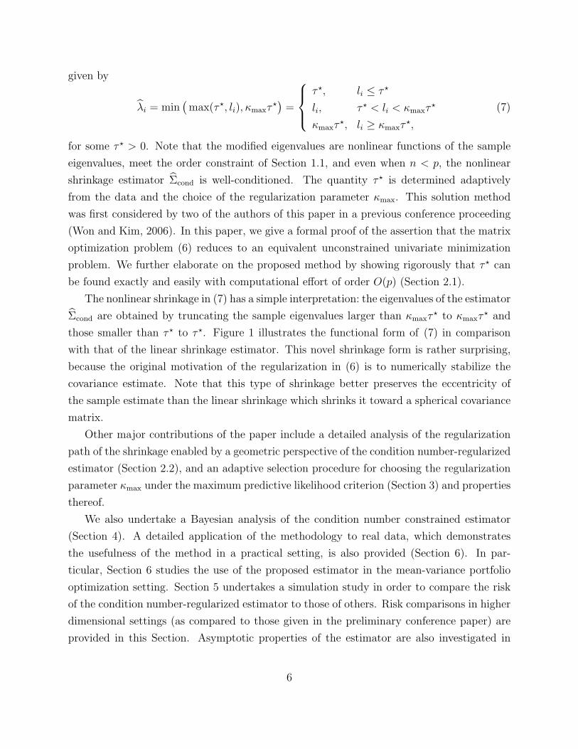
The nonlinear shrinkage in (7) has a simple interpretation: the eigenvalues of the estimator

Σcond are obtained by truncating the sample eigenvalues larger than κmaxτ⋆ to κmaxτ

⋆ and

those smaller than τ ⋆ to τ ⋆. Figure 1 illustrates the functional form of (7) in comparison

with that of the linear shrinkage estimator. This novel shrinkage form is rather surprising,

because the original motivation of the regularization in (6) is to numerically stabilize the

covariance estimate. Note that this type of shrinkage better preserves the eccentricity of

the sample estimate than the linear shrinkage which shrinks it toward a spherical covariance

matrix.

Other major contributions of the paper include a detailed analysis of the regularization

path of the shrinkage enabled by a geometric perspective of the condition number-regularized

estimator (Section 2.2), and an adaptive selection procedure for choosing the regularization

parameter κmax under the maximum predictive likelihood criterion (Section 3) and properties

thereof.

We also undertake a Bayesian analysis of the condition number constrained estimator

(Section 4). A detailed application of the methodology to real data, which demonstrates

the usefulness of the method in a practical setting, is also provided (Section 6). In par-

ticular, Section 6 studies the use of the proposed estimator in the mean-variance portfolio

optimization setting. Section 5 undertakes a simulation study in order to compare the risk

of the condition number-regularized estimator to those of others. Risk comparisons in higher

dimensional settings (as compared to those given in the preliminary conference paper) are

provided in this Section. Asymptotic properties of the estimator are also investigated in

6

mo

difie

de

ige

nlinear shrinkage

sample eigenvalues (li)

c

c

mo

difie

de

ige

n

condition number regularization

sample eigenvalues (li)

τ⋆

τ⋆

κmaxτ⋆

κmaxτ⋆

Figure 1: Comparison of eigenvalue shrinkage of the linear shrinkage estimator (left)and the condition number-constrained estimator (right).

Section 5.

2 Condition number-regularized covariance estimation

2.1 Derivation and characterization of solution

This section gives the derivation of the solution (7) of the condition number-regularized

covariance estimation problem as given in (6) and shows how to compute τ ⋆ given κmax.

Note that it suffices to consider the case κmax < l1/lp = cond(S), since otherwise, the

condition number constraint is already satisfied and the solution to (6) simply reduces to

the sample covariance matrix S.

It is well known that the log-likelihood (1) of a multivariate Gaussian covariance matrix

is a convex function of Ω = Σ−1. Note that Ω is the canonical parameter for the (Wishart)

natural exponential family associated with the likelihood in (1). Since cond(Σ) = cond(Ω),

it can be shown that the condition number constraint on Ω is equivalent to the existence of

u > 0 such that uI Ω κmaxuI, where A B denotes that B−A is positive semidefinite

(Boyd and Vandenberghe, 2004, Chap. 7). Therefore the covariance estimation problem (6)

is equivalent to

minimize tr(ΩS)− log detΩ

subject to uI Ω κmaxuI,(8)

7

where the variables are a symmetric positive definite p×p matrix Ω and a scalar u > 0. The

above problem in (8) is a convex optimization problem with p(p + 1)/2 + 1 variables, i.e.,

O(p2).

The following lemma shows that by exploiting structure of the problem it can be reduced

to a univariate convex problem, i.e., the dimension of the system is only of O(1) as compared

to O(p2).

Lemma 1. The optimization problem (8) is equivalent to the unconstrained univariate convex

optimization problem

minimize

p∑

i=1

J (i)κmax

(u), (9)

where

J (i)κmax

(u) = liµ⋆i (u)− log µ⋆

i (u) =

li(κmaxu)− log(κmaxu), u < 1/(κmaxli)

1 + log li, 1/(κmaxli) ≤ u ≤ 1/li

liu− log u, u > 1/li,

and

µ⋆i (u) = min

maxu, 1/li, κmaxu

, (10)

in the sense that the solution to (8) is a function of the solution u⋆ to (9), as follows.

Ω⋆ = Qdiag(µ⋆1(u

⋆), . . . , µ⋆p(u

⋆))QT ,

with Q defined as in (3).

Proof. The proof is given in the Appendix.

Characterization of the solution to (9) is given by the following theorem.

Theorem 1. Given κmax ≤ cond(S), the optimization problem (9) has a unique solution

given by

u⋆ =α⋆ + p− β⋆ + 1∑α⋆

i=1 li +∑p

i=β⋆ κmaxli, (11)

where α⋆ ∈ 1, . . . , p is the largest index such that 1/lα⋆ < u⋆ and β⋆ ∈ 1, . . . , p is the

smallest index such that 1/lβ⋆ > κmaxu⋆. The quantities α⋆ and β⋆ are not determined a

priori but can be found in O(p) operations on the sample eigenvalues l1 ≥ . . . ≥ lp. If

κmax > cond(S), the maximizer u⋆ is not unique but Σcond = S for all the maximizing values

of u.

8

Proof. The proof is given in the Appendix.

Comparing (10) to (7), it is immediately seen that

τ ⋆ = 1/(κmaxu⋆) =

∑α⋆

i=1 li/κmax +∑p

i=β⋆ li

α⋆ + p− β⋆ + 1. (12)

Note that the lower cutoff level τ ⋆ is an average of the (scaled and) truncated eigenvalues, in

which the eigenvalues above the upper cutoff level κmaxτ⋆ are shrunk by a factor of 1/κmax.

We highlight the fact that a reformulation of the original minimization into a univariate

optimization problem makes the proposed methodology very attractive in high dimensional

settings. The method is only limited by the complexity of spectral decomposition of the

sample covariance matrix (or the singular value decomposition of the data matrix). The

approach proposed here is therefore much faster than using interior point methods. We also

note that the condition number-regularized covariance estimator is orthogonally invariant:

if Σcond is the estimator of the true covariance matrix Σ, then UΣcondUT is the estimator of

the true covariance matrix UΣUT , for U orthogonal.

2.2 A geometric perspective on the regularization path

In this section, we shall show that a simple relaxation of the optimization problem (8)

provides an intuitive geometric perspective on the condition number-regularized estimator.

Consider the function

J(u, v) = minuIΩvI

(tr(ΩS)− log detΩ) (13)

defined as the minimum of the objective of (8) over a range uI Ω vI, where 0 < u ≤ v.

Note that the relaxation in (13) above differs from the original problem in the sense that the

optimization is no longer with respect to the variable u. In particular, u and v are fixed in

(13). By fixing u, the problem has now been significantly simplified. Paralleling Lemma 1,

it is easily shown that

J(u, v) =

p∑

i=1

minu≤µi≤v

(liµi − log µi).

Recall that the truncation range of the sample eigenvalues is therefore given by (1/v, 1/u).

Now for given u, let α ∈ 1, . . . , p be the largest index such that lα > 1/u and β ∈ 1, . . . , pbe the smallest index such that lβ < 1/v, i.e., the set of indexes where truncation at either

end of the spectrum first starts to become a binding constraint. With this convention it is

9

easily shown that J(u, v) can now be expressed in simpler form:

J(u, v) =

p∑

i=1

(liµ∗i (u, v)− log µ∗

i (u, v)) (14)

=α∑

i=1

(liu− log u) +

β−1∑

i=α+1

(1 + log li) +

p∑

i=β

(liv − log v), (15)

where

µ∗i (u, v) = min

maxu, 1/li, v

=

u, 1 ≤ i ≤ α

1/li, α < i < β

v, β ≤ i ≤ p.

(16)

Comparing (16) to (10), we observe that (Ω∗)−1, the covariance estimate whose inverse

achieves the minimum in (13), is obtained by truncating the eigenvalues of S greater than

1/u to 1/u, and less than 1/v to 1/v.

Furthermore, note that the function J(u, v) has the following properties:

1. J does not increase as u decreases and v increases simultaneously. This follows from

noting that simultaneously decreasing u and increasing v expands the domain of the

minimization in (13).

2. J(u, v) = J(1/l1, l/lp) for u ≤ 1/l1 and v ≥ 1/lp. Hence J(u, v) is constant on this part

of the domain. For these values of u and v, (Ω⋆)−1 = S.

3. J(u, v) is almost everywhere differentiable in the interior of the domain (u, v) : 0 <

u ≤ v, except for on the lines u = 1/l1, . . . , 1/lp and v = 1/l1, . . . , 1/lp. This follows

from noting the the indexes α and β changes their values only on these lines. Hence

the contribution to the three summands in (14) changes at these values.

We can now see the following obvious relation between the function J(u, v) and the

original problem (8): the solution to (8) as given by u⋆ is the minimizer of J(u, v) on the line

v = κmaxu, i.e., the original univariate optimization problem (9) is equivalent to minimizing

J(u, κmaxu). We denote this minimizer by u⋆(κmax) and investigate how u⋆(κmax) behaves

as κmax varies. The following proposition proves that u⋆(κmax) is monotone in κmax. This

result sheds light on the regularization path, i.e., the solution path of u⋆ as κmax varies.

Proposition 1. u⋆(κmax) is nonincreasing in κmax and v⋆(κmax) , κmaxu⋆(κmax) is nonde-

creasing, both almost surely.

10

Proof. The proof is given in the Appendix.

Remark The above proposition has a very natural and intuitive interpretation: when

the constraint on the condition number is relaxed to allow higher value of κmax, the gap

between u⋆ and v⋆ widens so that the ratio of v⋆ to u⋆ remains at κmax. This implies

that as κmax is increased, the lower truncation value u⋆ decreases and the higher truncation

value v⋆ increases. Proposition 1 can be equivalently interpreted by noting that the optimal

truncation range(τ ⋆(κmax), κmaxτ

⋆(κmax))of the sample eigenvalues is nested.

In light of the solution to the condition number-regularized covariance estimation prob-

lems in (7), Proposition 1 also implies that once an eigenvalue li is truncated for κmax = ν0,

then it remains truncated for all κmax < ν0. Hence the regularized eigenvalue estimates are

not only continuous, but they are also monotonic in the sense that they approach either

end of the truncation spectrum as the regularization parameter κmax is decreased to 1. This

monotonicity of the condition number-regularized estimates gives a desirable property that

is not always enjoyed by other regularized estimators, such as the lasso for instance (Personal

communications: Jerome Friedman, Department of Statistics, Stanford University).

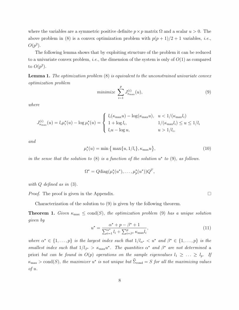
With the above theoretical knowledge on the regularization path of the sample eigenval-

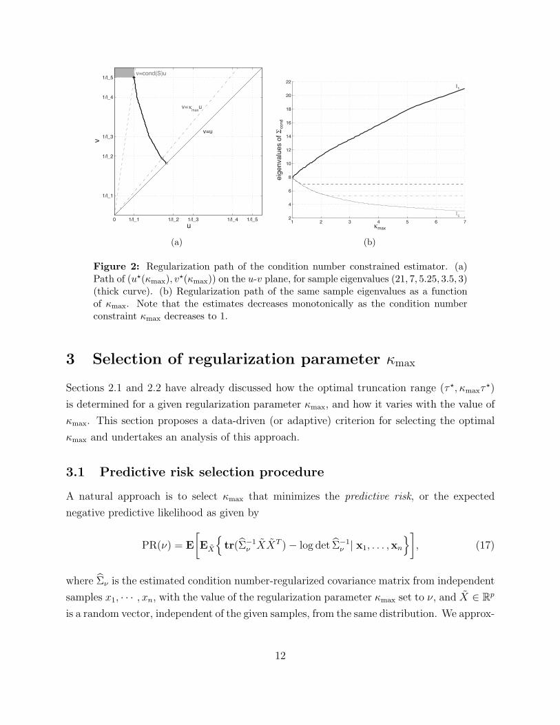
ues, we now provide an illustration of the regularization path; see Figure 2. More specif-

ically, consider the plot of the path of the optimal point (u⋆(κmax), v⋆(κmax)) on the u-v

plane from (u⋆(1), u⋆(1)) to (1/l1, 1/lp) when varying κmax from 1 to cond(S). The left

panel shows the path of (u⋆(κmax), v⋆(κmax)) on the u-v plane for the case where the sample

eigenvalues are (21, 7, 5.25, 3.5, 3). Here a point on the path represents the minimizer of

J(u, v) on a line v = κmaxu (hollow circle). The path starts from a point on the solid line

v = u (κmax = 1, square) and ends at (1/l1, 1/lp), where the dashed line v = cond(S) · upasses (κmax = cond(S), solid circle). Note that the starting point (κmax = 1) corresponds

to Σcond = γI for some data-dependent γ > 0 and the end point (κmax = cond(S)) to

Σcond = S. When κmax > cond(S), multiple values of u⋆ are achieved in the shaded region

above the dashed line, yielding nevertheless the same estimator S. The right panel of Figure

2 shows how the eigenvalues of the estimated covariance vary as a function of κmax. Here we

see that as the constraint is made stricter the eigenvalue estimates decrease monotonically.

Furthermore, the truncation range of the eigenvalues simultaneously decreases and remains

nested.

11

v=u

v=κmax

u

v=cond(S)u

u

v

0 1/l_1 1/l_2 1/l_3 1/l_4 1/l_5

1/l_1

1/l_2

1/l_3

1/l_4

1/l_5

(a)

1 2 3 4 5 6 72

4

6

8

10

12

14

16

18

20

22

κmax

eig

en

va

lue

s o

f Σ

co

nd

l1

l5

(b)

Figure 2: Regularization path of the condition number constrained estimator. (a)Path of (u⋆(κmax), v

⋆(κmax)) on the u-v plane, for sample eigenvalues (21, 7, 5.25, 3.5, 3)(thick curve). (b) Regularization path of the same sample eigenvalues as a functionof κmax. Note that the estimates decreases monotonically as the condition numberconstraint κmax decreases to 1.

3 Selection of regularization parameter κmax

Sections 2.1 and 2.2 have already discussed how the optimal truncation range (τ ⋆, κmaxτ⋆)

is determined for a given regularization parameter κmax, and how it varies with the value of

κmax. This section proposes a data-driven (or adaptive) criterion for selecting the optimal

κmax and undertakes an analysis of this approach.

3.1 Predictive risk selection procedure

A natural approach is to select κmax that minimizes the predictive risk, or the expected

negative predictive likelihood as given by

PR(ν) = E

[EX

tr(Σ−1

ν XXT )− log det Σ−1ν | x1, . . . ,xn

], (17)

where Σν is the estimated condition number-regularized covariance matrix from independent

samples x1, · · · , xn, with the value of the regularization parameter κmax set to ν, and X ∈ Rp

is a random vector, independent of the given samples, from the same distribution. We approx-

12

imate the predictive risk using K-fold cross validation. The K-fold cross validation approach

divides the data matrix X = (xT1 , · · · , xT

n ) into K groups so that XT =(XT

1 , . . . , XTK

)with

nk observations in the k-th group, k = 1, . . . , K. For the k-th iteration, each observation in

the k-th group Xk plays the role of X in (17), and the remaining K − 1 groups are used

together to estimate the covariance matrix, denoted by Σ[−k]ν . The approximation of the

predictive risk using the k-th group reduces to the predictive log-likelihood

lk(Σ[−k]

ν , Xk

)= −(nk/2)

[tr(

Σ[−k]ν

)−1XkX

Tk /nk

− log det

(Σ[−k]

ν

)−1].

The estimate of the predictive risk is then defined as

PR(ν) = − 1

n

K∑

k=1

lk(Σ[−k]

ν , Xk

). (18)

The optimal value for the regularization parameter κmax is selected as ν that minimizes

(18), i.e.,

κmax = inf(arg infν≥1

PR(ν)).

Note that the outer infimum is taken since lk(Σ

[−k]ν , Xk

)is constant for ν ≥ cond(S[−k]),

where S[−k] is the k-th fold sample covariance matrix based on the remaining K − 1 groups.

3.2 Properties of the optimal regularization parameter

We proceed to investigate the behavior of the selected regularization parameter κmax, both

theoretically and in simulations. We first note that κmax is a consistent estimator for the

true condition number κ . This fact is expressed below as one of the several properties of

κmax:

(P1) For a fixed p, as n increases, κmax approaches κ in probability, where κ is the condition

number of the true covariance matrix Σ.

This statement is stated formally below:

Theorem 2. For a given p,

limn→∞

pr(κmax = κ

)= 1.

Proof. The proof is given in Supplemental Section A.

13

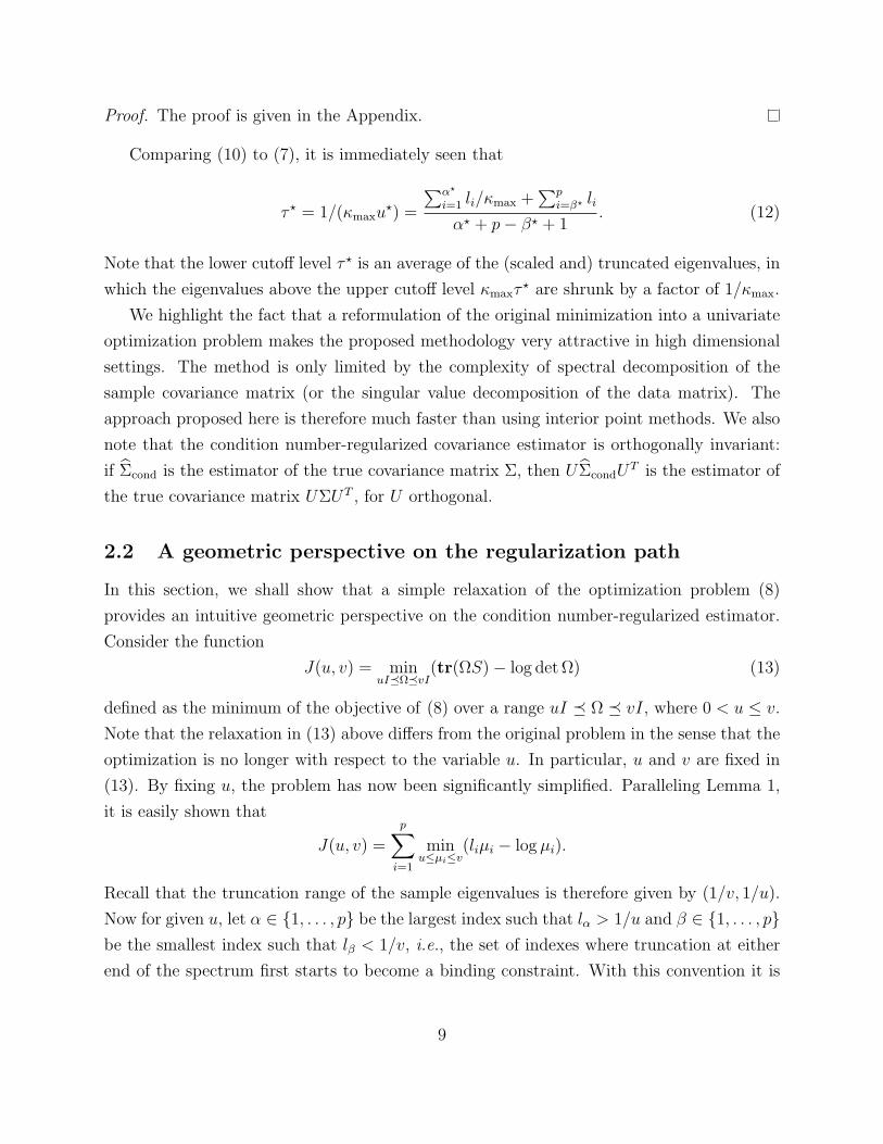
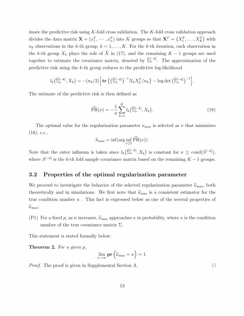
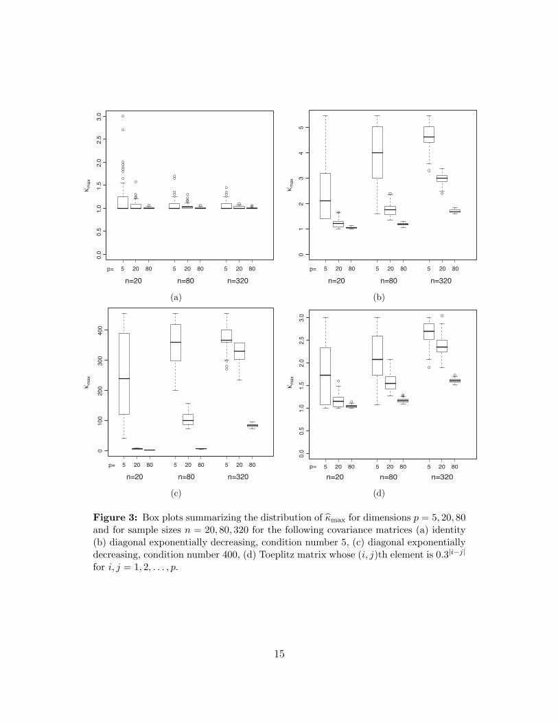
We further investigate the behavior of κmax in simulations. To this end, consider iid

samples from a zero-mean p-variate Gaussian distribution with the following covariance

matrices:

(i) Identity matrix in Rp.

(ii) diag(1, r, r2, . . . , rp), with condition number 1/rp = 5.

(iii) diag(1, r, r2, . . . , rp), with condition number 1/rp = 400.

(iv) Toeplitz matrix whose (i, j)th element is 0.3|i−j| for i, j = 1, . . . , p.

We consider different combinations of sample sizes and dimensions of the problem as given

by n = 20, 80, 320 and p = 5, 20, 80. For each of these cases 100 replicates are generated

and κmax computed with 5-fold cross validation. The behavior of κmax is plotted in Figure

3 and leads to insightful observations. A summary of the properties of the κmax is given in

(P2)–(P4) below:

(P2) If the condition number of the true covariance matrix remains finite as p increases,

then for a fixed n, κmax decreases.

(P3) If the condition number of the true covariance matrix remains finite as p increases,

then for a fixed n, κmax converges to 1.

(P4) The variance of κmax decreases as either n or p increases.

These properties are analogous to those of the optimal regularization parameter δ for the

linear shrinkage estimator (5), found using a similar predictive risk criterion (Warton, 2008).

4 Bayesian interpretation

In the same spirit as the Bayesian posterior mode interpretation of the LASSO (Tibshirani,

1996), we can draw parallels for the condition number regularized covariance estimator. The

condition number constraint given by λ1(Σ)/λp(Σ) ≤ κmax is similar to adding a penalty

term gmax(λ1(Σ)/λp(Σ)) to the likelihood equation for the eigenvalues:

maximize exp(−(n/2)

∑pi=1 li/λi

)(∏pi=1 λi

)−n/2exp(−gmax λ1/λp)

subject to λ1 ≥ · · · ≥ λp > 0

14

20 20 2080 80 80

0.0

0.5

1.0

1.5

2.0

2.5

3.0

p=

n=20 n=80 n=320

κm

ax

5 5 5

(a)5

20 20 2080 80 80p=

n=20 n=80 n=320κ

ma

x

43

21

0

55 5

(b)

20 20 2080 80 80

01

00

20

03

00

40

0

p=

n=20 n=80 n=320

κm

ax

55 5

(c)

520 20 2080 80 80

0.0

0.5

1.0

1.5

2.0

2.5

3.0

p=

n=20 n=80 n=320

κm

ax

5 5

(d)

Figure 3: Box plots summarizing the distribution of κmax for dimensions p = 5, 20, 80and for sample sizes n = 20, 80, 320 for the following covariance matrices (a) identity(b) diagonal exponentially decreasing, condition number 5, (c) diagonal exponentiallydecreasing, condition number 400, (d) Toeplitz matrix whose (i, j)th element is 0.3|i−j|

for i, j = 1, 2, . . . , p.

15

The above expression allows us to qualitatively interpret the condition number-regularized

estimator as the Bayes posterior mode under the following prior

π(λ1, . . . , λp) = exp(−gmax λ1/λp), λ1 ≥ · · · ≥ λp > 0 (19)

for the eigenvalues, and an independent Haar measure on the Stiefel manifold, as the prior

for the eigenvectors. The aforementioned prior on the eigenvalues has useful interesting

properties which help to explain the type of eigenvalue truncation described in previous

sections. We note that the prior is improper but the posterior is always proper.

Proposition 2. The prior on the eigenvalues in (19) is improper, whereas the posterior

yields a proper distribution. More formally,

∫

C

π(λ)dλ =

∫

C

exp(−gmax λ1/λp )dλ = ∞,

and

∫

C

π(λ)f(λ, l)dλ ∝∫

C

exp(−(n/2)

p∑

i=1

li/λi

)( p∏

i=1

λi

)−n/2exp(−gmax λ1/λp)dλ < ∞,

where λ = (λ1, . . . , λp) and C = λ : λ1 ≥ · · · ≥ λp > 0 .

Proof. The proof is given in Supplemental Section A.

The prior above puts the greatest mass around the region λ ∈ Rp : λ1 = · · · = λp which

consequently encourages “shrinking” or “pulling” the eigenvalues closer together. Note that

the support of both the prior and the posterior is the entire space of ordered eigenvalues.

Hence the prior simply by itself does not immediately yield a hard constraint on the condition

number. Evaluating the posterior mode yields an estimator that satisfies the condition

number constraint.

A clear picture of the regularization achieved by the prior above and its potential for

“eigenvalue shrinkage” emerges when compared to the other types of priors suggested in the

literature and the corresponding Bayes estimators. The standard MLE implies of course

a completely flat prior on the constrained space C. A commonly used inverse Wishart

conjugate prior Σ−1 ∼ Wishart(m, cI) yields a posterior mode which is a linear shrinkage

estimator (5) with δ = m/(n+m). Note however that the coefficients of the combination do

not depend of the data X, and are a function only of the sample size n and the degrees of

16

freedom or shape parameter from the prior, m. A useful prior for covariance matrices that

yields a data-dependent posterior mode is the reference prior proposed by Yang and Berger

(1994). For this prior, the eigenvalues are inversely proportional to the determinant of the

the covariance matrix, as given by∏p

i=1 λi, and also encourages shrinkage of the eigenvalues.

The posterior mode using this reference prior can be formulated similarly to that of condition

number regularization:

argmaxλ1≥...≥λp>0 exp(−(n/2)

p∑

i=1

li/λi

)( p∏

i=1

λi

)−n/2( p∏

i=1

λi

)−1

= argminλ1≥...≥λp>0 (n/2)

p∑

i=1

li/λi + ((n+ 2)/2)

p∑

i=1

log λi.

An examination of the penalty implied by the reference prior suggests that there is no direct

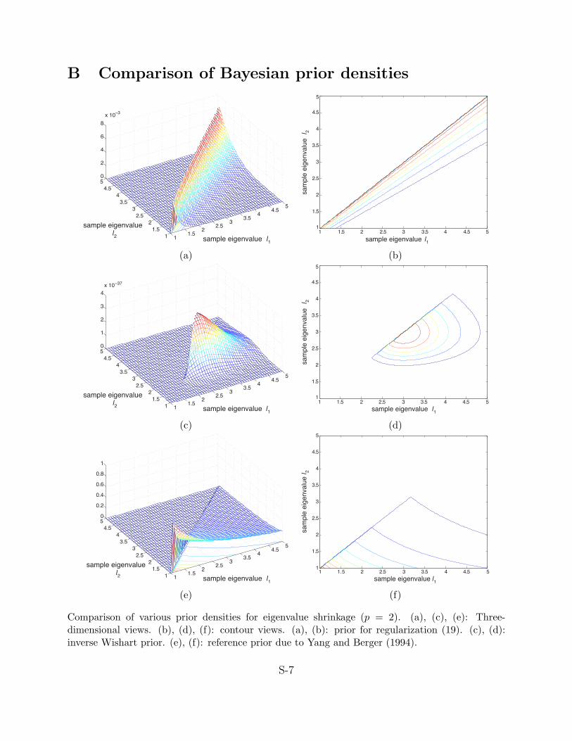
penalty on the condition number. In Supplemental Section B we illustrate the density of the

priors discussed above in the two-dimensional case. In particular, the density of the condition

number regularization prior places more emphasis on the line λ1 = λ2 thus “squeezing” the

eigenvalues together. This is in direct contrast with the inverse Wishart or reference priors

where this shrinkage effect is not as pronounced.

5 Decision-theoretic risk properties

5.1 Asymptotic properties

We now show that the condition number-regularized estimator Σcond has asymptotically

lower risk than the sample covariance matrix S with respect to entropy loss. Recall that the

entropy loss, also known as Stein’s loss, is defined as follows:

Lent(Σ,Σ) = tr(Σ−1Σ)− log det(Σ−1Σ)− p. (20)

Let λ1, . . . , λp, with λ1 ≥ · · · ≥ λp, denote the eigenvalues of the true covariance matrix Σ

and Λ = diag(λ1, . . . , λp

). Define λ =

(λ1, . . . , λp

), λ−1 =

(λ−11 , . . . , λ−1

p

), and κ = λ1

/λp.

First consider the trivial case when p > n. In this case, the sample covariance matrix

S is singular regardless of the singularity of Σ, and Lent(S,Σ) = ∞, whereas the loss and

therefore the risk of Σcond are always finite. Thus, Σcond has smaller entropy risk than S.

For p ≤ n, if the true covariance matrix has a finite condition number, it can be shown

17

that for a properly chosen κmax, the condition number-regularized estimator asymptotically

dominates the sample covariance matrix. This assertion is formalized below.

Theorem 3. Consider a class of covariance matrices D(κ, ω), whose condition numbers are

bounded above by κ and with minimum eigenvalue bounded below by ω > 0, i.e.,

D(κ, ω) =Σ = RΛRT : R orthogonal, Λ = diag(λ1, . . . , λp), ω ≤ λp ≤ . . . ≤ λ1 ≤ κω

.

Then, the following results hold.

(i) Consider the quantity Σ(κmax, ω) = Qdiag(λ1, . . . , λp)QT , where

λi =

ω, if li ≤ ω

li, if ω ≤ li < κmaxω

κmaxω, if li ≥ κmaxω,

and the sample covariance matrix given as S = Qdiag(l1, . . . , lp)QT , Q orthogonal,

l1 ≥ . . . ≥ lp. If the true covariance matrix Σ ∈ D(κmax, ω), then ∀ n, Σ(κmax, ω) has

a smaller entropy risk than S.

(ii) Consider a true covariance matrix Σ whose condition number is bounded above by κ,

i.e., Σ ∈ ⋃ω>0 D(κ, ω). If κmax ≥ κ(1−√

γ)−2

, then as p/n → γ ∈ (0, 1),

pr

(Σ ∈ D

(κmax, τ

⋆)

eventually

)= 1,

where τ ⋆ = τ ⋆(κmax) is given in (12).

Proof. The proof is given in Supplemental Section A.

Combining the two results above, we conclude that the estimator Σcond = Σ(κmax, τ⋆(κmax))

asymptotically has a lower entropy risk than the sample covariance matrix.

5.2 Finite sample performance

This section undertakes a simulation study in order to compare the finite-sample risks of the

condition number-regularized estimator Σcond with those of the sample covariance matrix

(S) and the linear shrinkage estimator (ΣLS) in the “large p, small n” setting. The regular-

ization parameter δ for ΣLS is chosen as prescribed in Warton (2008). The optimal Σcond is

18

calculated using the adaptive parameter selection method outlined in Section 3. Since Σcond

and ΣLS both select the regularization parameters similarly, i.e., by minimizing the empiri-

cal predictive risk (18), a meaningful comparison between two estimators can be made. We

consider two loss functions traditionally used in covariance estimation risk comparisons: (a)

entropy loss as given in (20) and (b) quadratic loss LQ(Σ,Σ) =∥∥ΣΣ−1 − I

∥∥2F.

Condition number regularization applies shrinkage to both ends of the sample eigenvalue

spectrum and does not affect the middle part, whereas linear shrinkage does this to the

entire spectrum uniformly. Therefore, it is expected that Σcond works well when a small

proportion of eigenvalues are found at the extremes. Such situations rise very naturally

when only a few eigenvalues explain most of the variation in data. To understand the

performance of the estimators in this context the following scenarios were investigated. We

consider diagonal matrices of dimensions p = 120, 250, 500 as true covariance matrices. The

eigenvalues (diagonal elements) are dichotomous, where the “high” values are (1−ρ)+ρp and

the “low” values are 1−ρ. For each p, we vary the composition of the diagonal elements such

that the high values take only one (singleton), 10%, 20%, 30%, and 40% of the total number

of p eigenvalues. The sample size n is chosen so that γ = p/n is approximately 1.25, 2, or 4.

Note that for a given p, the condition number of the true covariance matrices is held fixed

at 1 + pρ/(1 − ρ) regardless of the composition of eigenvalues. For each of the simulation

scenarios, we generate 1000 data sets and compute 1000 estimates of the true covariance

matrix. The risks are calculated by averaging the losses over these 1000 estimates.

Figure 4 presents the results for ρ = 0.1, and represents a large condition number. It is

observed that in general Σcond has less risk than ΣLS, which in turn has less risk than the

sample covariance matrix (entropy loss is not defined for the sample covariance matrix). This

phenomenon is most clear when the eigenvalue spectrum has a singleton in the extreme. In

this case, Σcond gives a risk reduction between 27 % and 67 % for entropy loss, and between

67 % and 91 % for quadratic loss. The risk reduction tends to be more pronounced in high

dimensional scenarios, i.e., for p large and n small. The performance of Σcond over ΣLS is

maintained until the “high” eigenvalues compose up to 30 % of the eigenvalue spectrum.

Comparing the two loss functions, risk reduction of Σcond is more distinct in quadratic loss.

We note that for quadratic loss with large p and large proportion of “high” eigenvalues, there

are cases that the sample covariance matrix can perform well.

As an example of a moderate condition number, results for the ρ = 0.5 case is given in

Supplemental Section C. General trends are the same as with the ρ = 0.1 case.

In summary, the risk comparison study provides a numerical evidence that condition

19

number regularization has merit when the true covariance matrix has a bimodal eigenvalue

distribution and/or the true condition number is large.

6 Application to portfolio selection

This section illustrates the merits of the condition number regularization in the context of

financial portfolio optimization, where a well-conditioned covariance estimator is necessary.

A portfolio refers to a collection of risky assets held by an institution or an individual.

Over the holding period, the return on the portfolio is the weighted average of the returns

on the individual assets that constitutes the portfolio, in which the weight associated with

each asset corresponds to its proportion in monetary terms. The objective of portfolio

optimization is to determine the weights that maximize the return on the portfolio. Since

the asset returns are stochastic, a portfolio always carries a risk of loss. Hence the objective

is to maximize the overall return subject to a given level of risk, or equivalently to minimize

risk for a given level of return. Mean-variance portfolio (MVP) theory (Markowitz, 1952)

uses the standard deviation of portfolio returns to quantify the risk. Estimation of the

covariance matrix of asset returns thus becomes critical in the MVP setting. An important

and difficult component of MVP theory is to estimate the expected return on the portfolio

(Luenberger, 1998; Merton, 1980). Since the focus of this paper lies in estimating covariance

matrices and not expected returns, we shall focus on determining the minimum variance

portfolio which only requires an estimate of the covariance matrix; see, e.g., Chan et al.

(1999). For this we shall use the condition number regularization, linear shrinkage and the

sample covariance matrix, in constructing a minimum variance portfolio. We compare their

respective performance over a period of more than 14 years.

6.1 Minimum variance portfolio rebalancing

We begin with a formal description of the minimum variance portfolio selection problem. The

universe of assets consists of p risky assets, denoted 1, . . . , p. We use ri to denote the return

of asset i over one period; that is, its change in price over one time period divided by its price

at the beginning of the period. Let Σ denote the covariance matrix of r = (r1, . . . , rp). We

employ wi to denote the weight of asset i in the portfolio held throughout the period. A long

position in asset i corresponds to wi > 0, and a short position corresponds to wi < 0. The

portfolio is therefore unambiguously represented by the vector of weights w = (w1, . . . , wp).

Without loss of generality, the budget constraint can be written as 1Tw = 1, where 1 is the

20

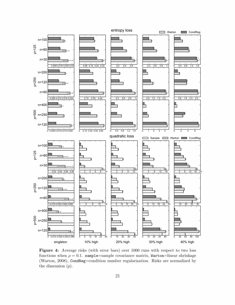
singleton 10% high 20% high 30% high 40% high

Figure 4: Average risks (with error bars) over 1000 runs with respect to two lossfunctions when ρ = 0.1. sample=sample covariance matrix, Warton=linear shrinkage(Warton, 2008), CondReg=condition number regularization. Risks are normalized bythe dimension (p).

21

vector of all ones. The risk of a portfolio is measured by the standard deviation (wTΣw)1/2

of its return.

Now the minimum variance portfolio selection problem can be formulated as

minimize wTΣw

subject to 1Tw = 1.(21)

This is a simple quadratic program that has an analytic solution w⋆ = (1TΣ−11)−1Σ−11. In

practice, the parameter Σ has to be estimated.

The standard portfolio selection problem described above assumes that the returns are

stationary, which is of course not realistic. As a way of dealing with the nonstationarity of

returns, we employ a minimum variance portfolio rebalancing (MVR) strategy as follows.

Let r(t) = (r(t)1 , . . . , r

(t)p ) ∈ R

p, t = 1, . . . , Ntot, denote the realized returns of assets at time

t (the time unit under consideration can be a day, a week, or a month). The periodic

minimum variance rebalancing strategy is implemented by updating the portfolio weights

every L time units, i.e., the entire trading horizon is subdivided into blocks each consisting

of L time units. At the start of each block, we determine the minimum variance portfolio

weights based on the past Nestim observations of returns. We shall refer to Nestim as the

estimation horizon size. The portfolio weights are then held constant for L time units during

these “holding” periods, i.e., during each of these blocks, and subsequently updated at the

beginning of the following one. For simplicity, we shall assume the entire trading horizon

consists of Ntot = Nestim + KL time units, for some positive integer K, i.e., there will be

K updates. (The last rebalancing is done at the end of the entire period, and so the out-

of-sample performance of the rebalanced portfolio for this holding period is not taken into

account.) We therefore have a series of portfolios w(j) = (1T (Σ(j))−11)−1(Σ(j))−11 over the

holding periods of [Nestim+1+(j−1)L,Nestim+jL], j = 1, . . . , K. Here Σ(j) is the covariance

matrix of the asset returns estimated from those over the jth holding period.

6.2 Empirical out-of-sample performance

In this empirical study, we use the 30 stocks that constituted the Dow Jones Industrial

Average as of July 2008 (Supplemental Section D.1 lists these 30 stocks). We used the

closing prices adjusted daily for all applicable splits and dividend distributions downloaded

from Yahoo! Finance (http://finance.yahoo.com/). The whole period considered in our

numerical study is from the trading date of December 14, 1992 to June 6, 2008 (this period

22

consists of 4100 trading days). We consider weekly returns: the time unit is 5 consecutive

trading days. We take

Ntot = 820, L = 15, Nestim = 15, 30, 45, 60.

To estimate the covariance matrices, we use the last Nestim weekly returns of the constituents

of the Dow Jones Industrial Average.3 The entire trading horizon corresponds to K = 48

holding periods, which span the dates from February 18, 1994 to June 6, 2008. In what

follows, we compare the MVR strategy where the covariance matrices are estimated using

the condition number regularization with those that use either the sample covariance matrix

or linear shrinkage. We employ two linear shrinkage schemes: that of Warton (2008) of

Section 5.2 and that of Ledoit and Wolf (2004). The latter is widely accepted as a well-

conditioned estimator in the financial literature.

Performance metrics

We use the following quantities in assessing the performance of the MVR strategies. For

precise formulae of these metrics, refer to Supplemental Section D.3.

• Realized return. The realized return of the portfolio over the trading period.

• Realized risk. The realized risk (return standard deviation) of the portfolio over the

trading period.

• Realized Sharpe ratio. The realized excess return, with respect to the risk-free rate,

per unit risk of the portfolio.

• Turnover. Amount of new portfolio assets purchased or sold over the trading period.

• Normalized wealth growth. Accumulated wealth yielded by the portfolio over the trad-

ing period when the initial budget is normalized to one, taking the transaction cost

into account.

• Size of the short side. The proportion of the short side (negative) weights to the sum

of the absolute weights of the portfolio.

We assume that the transaction costs are the same for the 30 stocks and set them to 30 basis

points. The risk-free rate is set at 5% per annum.

3Supplemental Section D.2 shows the periods determined by the choice of the parameters.

23

Comparison results

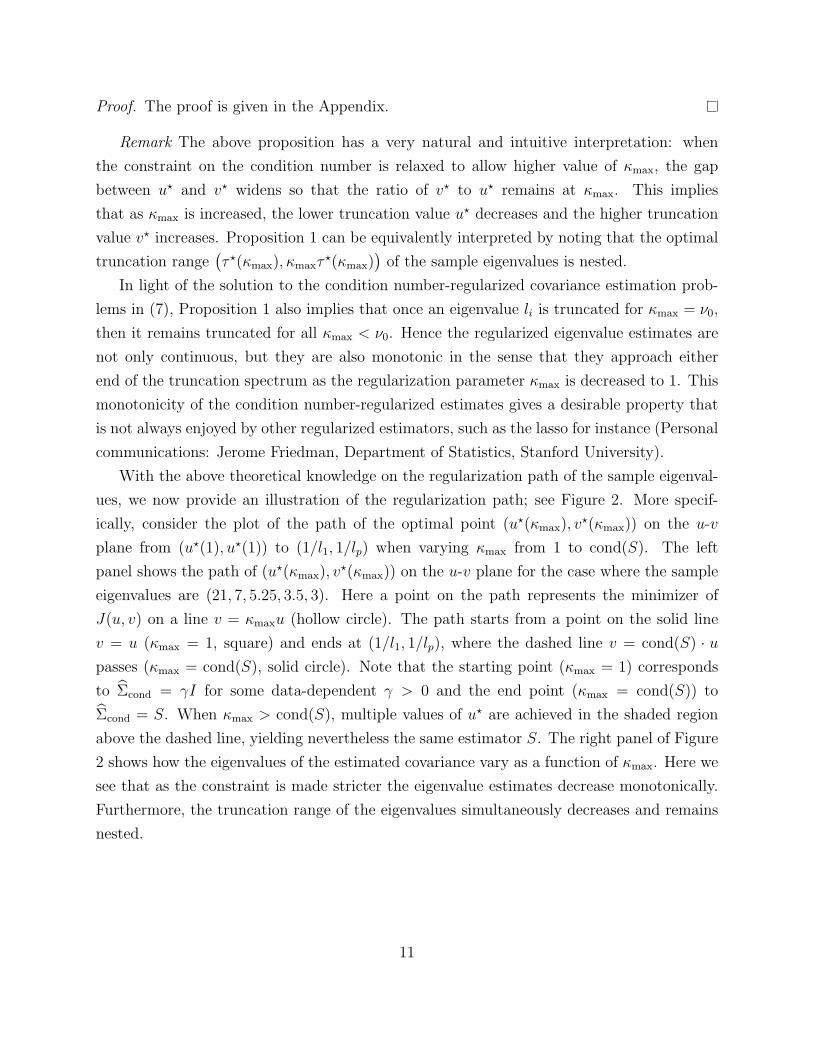
Figure 5 shows the normalized wealth growth over the trading horizon for four different

values of Nestim. The sample covariance matrix failed in solving (21) for Nestim = 15 because

of its singularity and hence is omitted in this figure. The MVR strategy using the condition

number-regularized covariance matrix delivers higher growth as compared to using the sam-

ple covariance matrix, linear shrinkage or index tracking in this performance metric. The

higher growth is realized consistently across the 14 year trading period and is regardless of

the estimation horizon. A trading strategy based on the condition number-regularized co-

variance matrix consistently performs better than the S&P 500 index and can lead to profits

as much as 175% more than its closest competitor.

A useful result appears after further analysis. There is no significant difference between

the condition number regularization approach and the two linear shrinkage schemes in terms

of the realized return, risk, and Sharpe ratio. Supplemental Section D.4 summarizes these

metrics for each estimator respectively averaged over the trading period. For all values of

Nestim, the average differences of the metrics between the two regularization schemes are

within two standard errors of those. Hence the condition number regularized estimator de-

livers better normalized wealth growth than the other estimators but without compromising

on other measures such as volatility.

The turnover of the portfolio seems to be one of the major driving factors of the difference

in wealth growth. In particular, the MVR strategy using the condition number-regularized

covariance matrix gives far lower turnover and thus more stable weights than when using the

linear shrinkage estimator or the sample covariance matrix. (See Supplemental Section D.5

for plots.) A lower turnover also implies less transaction costs, thereby also partially con-

tributing to the higher wealth growth. Note that there is no explicit limit on turnover.

The stability of the MVR portfolio using the condition number regularization appears to be

related to its small size of the short side (reported in Supplemental Section D.6). Because

stock borrowing is expensive, the condition number regularization based strategy can be

advantageous in practice.

Appendix

Proof of Lemma 1. Recall the spectral decomposition of the sample covariance matrix S =

QLQT , with L = diag(l1, . . . , lp) and l1 ≥ . . . ≥ lp ≥ 0. From the objective function in

(8), suppose the variable Ω has the spectral decomposition RMRT , with R orthogonal and

24

1/1996 1/1998 1/2000 1/2002 1/2004 1/2006 1/2008−1

0

1

2

3

4

5

6

7

time

normalized wealth growth

LW

Warton

condreg

S&P500

(a) Nestim = 15

1/1996 1/1998 1/2000 1/2002 1/2004 1/2006 1/2008−1

0

1

2

3

4

5

6

7

time

normalized wealth growth

sample

LW

Warton

condreg

S&P500

(b) Nestim = 30

1/1996 1/1998 1/2000 1/2002 1/2004 1/2006 1/2008−1

0

1

2

3

4

5

6

7

time

normalized wealth growth

sample

LW

Warton

condreg

S&P500

(c) Nestim = 45

1/1996 1/1998 1/2000 1/2002 1/2004 1/2006 1/2008−1

0

1

2

3

4

5

6

7

time

normalized wealth growth

sample

LW

Warton

condreg

S&P500

(d) Nestim = 60

Figure 5: Normalized wealth growth results of the minimum variance rebalancingstrategy for various estimation horizon sizes over the trading period from February 18,1994 through June 6, 2008. sample=sample covariance matrix, LW=linear shrinkage(Ledoit and Wolf, 2004), Warton=linear shrinkage (Warton, 2008), condreg=conditionnumber regularization. For comparison, the S&P 500 index for the same period (i.e.,index tracking), with the initial price normalized to 1, is also plotted.

25

M = diag(µ1, . . . , µp), µ1 ≤ . . . ≤ µp. Then the objective function in (8) can be written as

tr(ΩS)− log det(Ω) = tr(RMRTQLQT )− log det(RMRT )

= l(R,M)

≥ tr(ML)− log detM = l(Q,M),

with equality in the last line when R = Q (Farrell, 1985, Ch. 14). Hence (8) amounts to

minimize∑p

i=1(liµi − log µi)

subject to u ≤ µ1 ≤ · · · ≤ µp ≤ κmaxu, i = 1, . . . , p,(22)

with the optimization variables µ1, . . . , µp and u.

For the moment we shall ignore the order constraints among the eigenvalues. Then

problem (22) becomes separable in µ1, . . . , µp. Call this related problem (22*). For a fixed u,

the minimizer of each summand of the objective function in (22) without the order constraints

is given as

µ⋆i (u) = argmin

u≤µi≤κmaxu(liµi − log µi) = min

maxu, 1/li, κmaxu

. (23)

Note that (23) however satisfies the order constraints. In other words, µ⋆1(u) ≤ . . . ≤ µ⋆

p(u)

for all u. Therefore (22*) is equivalent to (22). Plugging (23) in (22) removes the constraints

and the objective function reduces to a univariate one:

Jκmax(u) ,

p∑

i=1

J (i)κmax

(u), (24)

where

J (i)κmax

(u) = liµ⋆i (u)− log µ⋆

i (u) =

li(κmaxu)− log(κmaxu), u < 1/(κmaxli)

1 + log li, 1/(κmaxli) ≤ u ≤ 1/li

liu− log u, u > 1/li.

The function (24) is convex, since each J(i)κmax

is convex in u.

Proof of Theorem 1. The function J(i)κmax

(u) is convex and is constant on the interval [1/(κmaxli), 1/li].

Thus, the function Jκmax(u) ,

∑pi=1 J

(i)κmax

(u) has a region on which it is a constant if and

26

only if [1/(κmaxl1), 1/l1

]⋂[1/(κmaxlp), 1/lp

]6= ∅,

or equivalently, κmax > cond(S). Therefore, provided that κmax ≤ cond(S), the convex

function Jκmax(u) does not have a region on which it is constant. Since Jκmax

(u) is strictly

decreasing for 0 < u < 1/(κmaxl1) and strictly increasing for u > 1/lp, it has a unique

minimizer u⋆. If κmax > cond(S), the maximizer u⋆ may not be unique because Jκmax(u) has

a plateau. However, since the condition number constraint becomes inactive, Σcond = S for

all the maximizers.

Now assume that κmax ≤ cond(S). For α ∈ 1, . . . , p− 1 and β ∈ 2, . . . , p, define the

following two quantities.

uα,β =α + p− β + 1∑α

i=1 li +∑p

i=β κmaxliand vα,β = κmaxuα,β.

By construction, uα,β coincides with u⋆ if and only if

1/lα < uα,β ≤ 1/lα+1 and 1/lβ−1 ≤ κmaxuα,β < 1/lβ. (25)

Consider a set of rectangles Rα,β in the uv-plane such that

Rα,β = (u, v) : 1/lα < u ≤ 1/lα+1 and 1/lβ−1 ≤ v < 1/lβ.

Then condition (25) is equivalent to

(uα,β, vα,β) ∈ Rα,β (26)

in the uv-plane. Since Rα,β partitions (u, v) : 1/l1 < u ≤ 1/lp and 1/l1 ≤ v < 1/lpand (uα,β, vα,β) is on the line v = κmaxu, an obvious algorithm to find the pair (α, β) that

satisfies the condition (26) is to keep track of the rectangles Rα,β that intersect this line.

To understand that algorithm takes O(p) operations, start from the origin of the uv-plane,

increase u and v along the line v = κmaxu. Since κmax > 1, if the line intersects Rα,β, then

the next intersection occurs in one of the three rectangles: Rα+1,β, Rα,β+1, and Rα+1,β+1.

Therefore after finding the first intersection (which is on the line u = 1/l1), the search

requires at most 2p tests to satisfy condition (26). Finding the first intersection takes at

most p tests.

27

Proof of Proposition 1. Recall that, for κmax = ν0,

u⋆(ν0) =α + p− β + 1∑αi=1 li + ν0

∑pi=β li

and

v⋆(ν0) = ν0u⋆(ν0) =

α + p− β + 11ν0

∑αi=1 li +

∑pi=β li

,

where α = α(ν0) ∈ 1, . . . , p is the largest index such that 1/lα < u⋆(ν0) and β = β(ν0) ∈1, . . . , p is the smallest index such that 1/lβ > ν0u

⋆(ν0). Then

1/lα < u⋆(ν0) ≤ 1/lα+1

and

1/lβ−1 ≤ v⋆(ν0) < 1/lβ.

The lower and upper bounds u⋆(ν0) and v⋆(ν0) of the reciprocal sample eigenvalues can be

divided into four cases:

1. 1/lα < u⋆(ν0) < 1/lα+1 and 1/lβ−1 < v⋆(ν0) < 1/lβ.

We can find ν > ν0 such that

1/lα < u⋆(ν) ≤ 1/lα+1

and

1/lβ−1 ≤ v⋆(ν) < 1/lβ.

Therefore,

u⋆(ν) =α + p− β + 1∑αi=1 li + ν

∑pi=β li

<α + p− β + 1∑αi=1 li + ν0

∑pi=β li

= u⋆(ν0)

and

v⋆(ν) =α + p− β + 1

1ν0

∑αi=1 li +

∑pi=β li

>α + p− β + 1

1ν

∑αi=1 li +

∑pi=β li

= v⋆(ν0).

2. u⋆(ν0) = 1/lα+1 and 1/lβ−1 < v⋆(ν0) < 1/lβ.

Suppose u⋆(ν) > u⋆(ν0). Then we can find ν > ν0 such that α(ν) = α(ν0) + 1 = α+ 1

28

and β(ν) = β(ν0) = β. Then,

u⋆(ν) =α + 1 + p− β + 1∑α+1

i=1 li + ν∑p

i=β li.

Therefore,

1

u⋆(ν0)− 1

u⋆(ν)= 1/lα+1 −

∑α+1i=1 li + ν

∑pi=β li

α + 1 + p− β + 1

=(α + p− β + 1)lα+1 − (

∑α+1i=1 li + ν

∑pi=β li)

α + 1 + p− β + 1> 0,

or

lα+1 >

∑α+1i=1 li + ν

∑pi=β li

α + p− β + 1>

∑α+1i=1 li + ν0

∑pi=β li

α + p− β + 1= lα+1,

which is a contradiction. Therefore, u⋆(ν) ≤ u⋆(ν0).

Now, we can find ν > ν0 such that α(ν) = α(ν0) = α and β(ν) = β(ν0) = β. This

reduces to case 1.

3. 1/lα < u⋆(ν0) < 1/lα+1 and v⋆(ν0) = 1/lβ−1.

Suppose v⋆(ν) < v⋆(ν0). Then we can find ν > ν0 such that α(ν) = α(ν0) = α and

β(ν) = β(ν0)− 1 = β − 1. Then,

v⋆(ν) =α + p− β + 2

1ν

∑αi=1 li +

∑pi=β−1 li

.

Therefore,

1

v⋆(ν0)− 1

v⋆(ν)= 1/lβ−1 −

∑αi=1 li + ν

∑pi=β−1 li

α + p− β + 2

=(α + p− β + 1)lβ−1 − (

∑αi=1 li + ν

∑pi=β li)

α + p− β + 2< 0,

or

lβ−1 <

∑αi=1

1νli +

∑pi=β−1 li

α + p− β + 1<

∑α+1i=1

1ν0li +

∑pi=β li

α + p− β + 1= lβ−1,

which is a contradiction. Therefore, v⋆(ν) ≥ v⋆(ν0).

Now, we can find ν > ν0 such that α(ν) = α(ν0) = α and β(ν) = β(ν0) = β. This

reduces to case 1.

29

4. u⋆(ν0) = 1/lα+1 and v⋆(ν0) = 1/lβ−1. 1/lα+1 = u⋆(ν0) = v⋆(ν0)/ν0 = 1/(ν0lβ−1). This

is a measure zero event and does not affect the conclusion.

Supplemental materials Accompanying supplemental materials contain additional proofs

of Theorems 2 and 3, and Proposition 2; additional figures illustrating Bayesian prior densi-

ties; additional figure illustrating risk simulations; details of the empirical minimum variance

rebalancing study.

Acknowledgments We thank the editor and the associate editor for useful comments

that improved the presentation of the paper. J. Won was partially supported by the US

National Institutes of Health (NIH) (MERIT Award R37EB02784) and by the US National

Science Foundation (NSF) grant CCR 0309701. J. Lim’s research was supported by the

Basic Science Research Program through the National Research Foundation of Korea (NRF)

funded by the Ministry of Education, Science and Technology (grant number: 2010-0011448).

B. Rajaratnam was supported in part by NSF under grant nos. DMS-09-06392, DMS-CMG

1025465, AGS-1003823, DMS-1106642 and grants NSA H98230-11-1-0194, DARPA-YFA

N66001-11-1-4131, and SUWIEVP10-SUFSC10-SMSCVISG0906.

References

Banerjee, O., L. El Ghaoui, and A. D’Aspremont (2008). Model Selection Through SparseMaximum Likelihood Estimation for Multivariate Gaussian or Binary Data. Journal ofMachine Learning Research 9, 485–516.

Boyd, S. and L. Vandenberghe (2004). Convex Optimization. Cambridge University Press.

Chan, N., N. Karceski, and J. Lakonishok (1999). On portfolio optimization: Forecastingcovariances and choosing the risk model. Review of Financial Studies 12 (5), 937–974.

Daniels, M. and R. Kass (2001). Shrinkage estimators for covariance matrices. Biometrics 57,1173–1184.

Dempster, A. P. (1972). Covariance Selection. Biometrics 28 (1), 157–175.

Dey, D. K. and C. Srinivasan (1985). Estimation of a covariance matrix under Stein’s loss.The Annals of Statistics 13 (4), 1581–1591.

Farrell, R. H. (1985). Multivariate calculation. Springer-Verlag New York.

30

Friedman, J., T. Hastie, and R. Tibshirani (2008). Sparse inverse covariance estimation withthe graphical lasso. Biostatistics 9 (3), 432–441.

Haff, L. R. (1991). The variational form of certain Bayes estimators. The Annals of Statis-tics 19 (3), 1163–1190.

Hero, A. and B. Rajaratnam (2011). Large-scale correlation screening. Journal of theAmerican Statistical Association 106 (496), 1540–1552.

Hero, A. and B. Rajaratnam (2012). Hub discovery in partial correlation graphs. InformationTheory, IEEE Transactions on 58 (9), 6064–6078.

James, W. and C. Stein (1961). Estimation with quadratic loss. In Proceedings of theFourth Berkeley Symposium on Mathematical Statistics and Probability, Stanford, Califor-nia, United States, pp. 361–379.

Khare, K. and B. Rajaratnam (2011). Wishart distributions for decomposable covariancegraph models. The Annals of Statistics 39 (1), 514–555.

Ledoit, O. and M. Wolf (2003, December). Improved estimation of the covariance ma-trix of stock returns with an application to portfolio selection. Journal of EmpiricalFinance 10 (5), 603–621.

Ledoit, O. and M. Wolf (2004). A well-conditioned estimator for large-dimensional covariancematrices. Journal of Multivariate Analysis 88, 365–411.

Ledoit, O. and M. Wolf (2012, July). Nonlinear shrinkage estimation of large-dimensionalcovariance matrices. The Annals of Statistics 40 (2), 1024–1060.

Letac, G. and H. Massam (2007). Wishart distributions for decomposable graphs. TheAnnals of Statistics 35 (3), 1278–1323.

Lin, S. and M. Perlman (1985). A Monte-Carlo comparison of four estimators of a covariancematrix. Multivariate Analysis 6, 411–429.

Luenberger, D. G. (1998). Investment science. Oxford University Press New York.

Markowitz, H. (1952). Portfolio selection. Journal of Finance 7 (1), 77–91.

Merton, R. (1980). On estimating expected returns on the market: An exploratory investi-gation. Journal of Financial Economics 8, 323–361.

Michaud, R. O. (1989). The Markowitz Optimization Enigma: Is Optimized Optimal. Fi-nancial Analysts Journal 45 (1), 31–42.

Peng, J., P. Wang, N. Zhou, and J. Zhu (2009). Partial correlation estimation by joint sparseregression models. Journal of the American Statistical Association 104 (486), 735–746.

31

Pourahmadi, M., M. J. Daniels, and T. Park (2007, March). Simultaneous modelling ofthe cholesky decomposition of several covariance matrices. Journal of Multivariate Anal-ysis 98 (3), 568–587.

Rajaratnam, B., H. Massam, and C. Carvalho (2008). Flexible covariance estimation ingraphical Gaussian models. The Annals of Statistics 36 (6), 2818–2849.

Sheena, Y. and A. Gupta (2003). Estimation of the multivariate normal covariance matrixunder some restrictions. Statistics & Decisions 21, 327–342.

Stein, C. (1956). Some problems in multivariate analysis Part I. Technical Report 6, Dept.of Statistics, Stanford University.

Stein, C. (1975). Estimation of a covariance matrix. Reitz Lecture, IMS-ASA Annual Meet-ing .

Stein, C. (1986). Lectures on the theory of estimation of many parameters (English transla-tion). Journal of Mathematical Sciences 34 (1), 1373–1403.

Tibshirani, R. (1996). Regression shrinkage and selection via the lasso. Journal of the RoyalStatistical Society. Series B (Methodological) 58 (1), 267–288.

Warton, D. I. (2008). Penalized Normal Likelihood and Ridge Regularization of Correlationand Covariance Matrices. Journal of the American Statistical Association 103 (481), 340–349.

Won, J. H. and S.-J. Kim (2006). Maximum Likelihood Covariance Estimation with aCondition Number Constraint. In Proceedings of the Fortieth Asilomar Conference onSignals, Systems and Computers, pp. 1445–1449.

Yang, R. and J. O. Berger (1994). Estimation of a covariance matrix using the referenceprior. The Annals of Statistics 22 (3), 1195–1211.

32

A Additional proofs

Proof of Theorem 2. Suppose the spectral decomposition of the k-th fold covariance matrix esti-

mate Σ[−k]ν , with κmax = ν, is given by

Σ[−k]ν = Q[−k]diag

(λ[−k]1 , . . . , λ[−k]

p

)(Q[−k]

)T

with

λ[−k]i =

v[−k]∗ if l[−k]i < v[−k]∗

l[−k]i if v[−k]∗ ≤ l

[−k]i < νv[−k]∗

νv[−k]∗ if l[−k]i ≥ νv[−k]∗,

where l[−k]i is the i-th largest eigenvalue of the k-th fold sample covariance matrix S[−k], and v[−k]∗ is

obtained by the method described in Section 2. Since Σ[−k]ν = S[−k] if ν ≥ l

[−k]1 /l

[−k]p = cond(S[−k]),

κmax ≤ maxk=1,...,K

cond(S[−k]). (27)

The right hand side of (27) converges in probability to the condition number κ of the true covariancematrix, as n increases while p is fixed. Hence,

limn→∞

P(κmax ≤ κ

)= 1.

We now show thatlimn→∞

P(κmax ≥ κ

)= 1.

by showing that PR(ν)is an asymptotically decreasing function in ν.

Recall that

PR(ν)= − 1

n

K∑

k=1

lk(Σ[−k]ν , Xk

),

where

lk(Σ[−k]ν , Xk

)= −(nk/2)

[tr(

Σ[−k]ν

)−1XkX

Tk /nk

− log det

(Σ[−k]ν

)−1],

which, by the definition of Σ[−k]ν , is everywhere differentiable but at a finite number of points.

S-1

To see the asymptotic monotonicity of PR(ν), consider the derivative −∂lk(Σ[−k]ν , Xk

)/∂ν:

−∂lk(Σ[−k]ν , Xk

)

∂ν=nk2

[tr

((Σ[−k]ν

)−1∂Σ[−k]ν

∂ν

)+ tr

∂(Σ[−k]ν

)−1

∂ν

(XkX

Tk

/nk

)]

=nk2

[tr

((Σ[−k]ν

)−1∂Σ[−k]ν

∂ν

)+ tr

∂(Σ[−k]ν

)−1

∂νΣ[−k]ν

+ tr

∂(Σ[−k]ν

)−1

∂ν

(XkX

Tk

/nk − Σ[−k]

ν

)]

=nk2

[∂

∂νtr((

Σ[−k]ν

)−1Σ[−k]ν

)+ tr

∂(Σ[−k]ν

)−1

∂ν

(XkX

Tk

/nk − Σ[−k]

ν

)]

=nk2

tr

∂Σ−1

ν

∂ν

(XkX

Tk

/nk − Σ[−k]

ν

).

As n (hence nk) increases, Σ[−k]ν converges almost surely to the inverse of the solution to the

following optimization problem

minimize tr(ΩΣ)− log detΩsubject to cond(Ω) ≤ ν,

with Σ and ν replacing S and κmax in (8). We denote the limit of Σ[−k]ν by Σν . For the spectral

decomposition of ΣΣ = R diag

(λ1, . . . , λp

)RT , (28)

Σν is given asΣν = R diag

(ψ1(ν), . . . , ψp(ν)

)RT , (29)

where, for some τ(ν) > 0,

ψi(ν) =

τ(ν) if λi ≤ τ(ν)λi if τ(ν) < λi ≤ ντ(ν)ντ(ν), if ντ(ν) < λi.

Recall from Proposition 1 that τ(ν) is decreasing in ν and ντ(ν) is increasing.Let ck be the limit of nk

/(2n) when both n and nk increases. Then, XkX

Tk

/nk converges almost

surely to Σ. Thus,

− 1

n

∂lk(Σ[−k]ν , Xk

)

∂ν→ ck tr

∂Σ−1

ν

∂ν

(Σ− Σν

), almost surely. (30)

If ν ≥ κ, then Σν = Σ, and the RHS of (30) degenerates to 0. Now consider the case thatν < κ. From (29),

∂Σ−1ν

∂ν= R

∂Ψ−1

∂νRT = R diag

(∂ψ−1

1

∂ν, . . . ,

∂ψ−1p

∂ν

)RT ,

S-2

where

∂ψ−1i

∂ν=

− 1τ(ν)2

∂τ(ν)∂ν (≥ 0) if λi ≤ τ(ν)

0 if τ(ν) < λi ≤ ντ(ν)

− 1ν2τ(ν)2

∂(ντ(ν))∂ν (≤ 0) if ντ(ν) < λi.

From (28) and (29),Σ− Σν = Rdiag

(λ1 − ψ1, . . . , λp − ψp

)RT ,

where

λi − ψi =

λi − τ(ν) (≤ 0) if λi ≤ τ(ν)0 if λi ≤ ντ(ν)λi − ντ(ν) (≥ 0) if ντ(ν) < λi.

Therefore,

tr

∂Σ−1

ν

∂ν

(Σ− Σν

)=∑

i

∂ψ−1i

∂ν· (λi − ψi) ≤ 0.

In other words, the RHS of (30) is less than 0 and the almost sure limit of PR(ν) is decreasing inν.

By definition, PR(κmax) ≤ PR(κ). From this and the asymptotic monotonicity of PR(ν), weconclude that

limn→∞

pr(κmax ≥ κ

)= 1.

Proof of Proposition 2. We are given that

π(λ1, . . . , λp) = exp

(−gmax

λ1λp

)λ1 ≥ · · · ≥ λp > 0.

Now ∫

Cπ(λ1, . . . , λp)dλ =

∫

Cexp

(−gmax

λ1λp

)dλ,

where C = λ1 ≥ · · · ≥ λp > 0.Let us now make the following change of variables: xi = λi − λi+1 for i = 1, 2, .., p − 1, and

xp = λp. The inverse transformation yields λi =∑p

j=i xj for i = 1, 2, .., p. It is straightforward toverify that the Jacobian of this transformation is given by |J | = 1.

S-3

Now we can therefore rewrite the integral above as

∫

Cexp

(−gmax

λ1λp

)dλ =

∫

Rp

1

exp

(−gmax

x1 + · · ·+ xpxp

)dx1 · · · dxp

= e−gmax

∫ [p−1∏

i=1

∫exp

(−gmax

xixp

)dxi

]dxp

= e−gmax

∫ ∞

0

(xpgmax

)p−1

dxp

=e−gmax

gp−1max

∫ ∞

0xp−1p dxp

= ∞.

To prove that the posterior yields a proper distribution we proceed as follows:

∫

Cπ(λ)f(λ, l)dλ

∝∫

Cexp

(−n2

p∑

i=1

liλi

)(p∏

i=1

λi

)−n2

exp

(−gmax

λ1λp

)dλ

≤∫

Cexp

(−n2

p∑

i=1

lpλi

)(p∏

i=1

λi

)−n2

exp

(−gmax

λ1λp

)dλ as lp ≤ li ∀i = 1, . . . , p

≤∫

Cexp

(−n2

p∑

i=1

lpλi

)(p∏

i=1

λi

)−n2

e−gmaxdλ asλ1λp

≥ 1

≤ e−gmax

p∏

i=1

(∫ ∞

0exp

(−n2

lpλi

)λ−n

2

i dλi

).

The above integrand is the density of the inverse gamma distribution and therefore the correspond-ing integral above has a finite normalizing constant and thus yielding a proper posterior.

Proof of Theorem 3. (i) The conditional risk of Σ(κmax, ω), given the sample eigenvalues l =(l1, . . . , lp), is

E(Lent(Σ(κmax, ω),Σ)

∣∣l)

=

p∑

i=1

λiE

(aii(Q)

∣∣l)− log λi

+ log detΣ− p,

where aii(Q) =∑p

j=1 q2jiλ

−1j and qji is the (j, i)-th element of the orthogonal matrix Q. This is

because

Lent

(Σ(κmax, ω),Σ

)= tr

(ΛA(Q)

)− log det Λ + log detΣ− p

=

p∑

i=1

λiaii(Q)− log λi

+ log detΣ− p, (31)

S-4

where A(Q) = QTΣ−1Q.In (31), the summand has the form

xE(aii(Q)

∣∣l)− log x

whose minimum is achieved at x = 1/E(aii(Q)

∣∣l). Since

∑pj=1 q

2ji = 1 and Σ−1 ∈ D

(κmax, 1/(κmaxω)

)

if and only if Σ ∈ D(κmax, ω

), we have 1/(κmaxω) ≤ aii(Q) ≤ 1/ω. Hence 1/E

(aii(Q)

∣∣l)lies be-

tween ω and κmaxω almost surely. Therefore,

1. If li ≤ ω, then λi = ω and

λiE(aii(Q)

∣∣l)− log λi ≤ liE

(aii(Q)

∣∣l)− log li.

2. If ω ≤ li < κmaxω, then λi = li and

λiE(aii(Q)

∣∣l)− log λi = liE

(aii(Q)

∣∣l)− log li.

3. If li ≥ κmaxω, then λi = κmaxω and

λiE(aii(Q)

∣∣l)− log λi ≤ liE

(aii(Q)

∣∣l)− log li.

Thus,p∑

i=1

λiE

(aii(Q)

∣∣l)− log λi

≤

p∑

i=1

liE

(aii(Q)

∣∣l)− log li

and the risk with respect to the entropy loss is

Rent

(Σ(κmax, ω)

)= E

[ p∑

i=1

λiE

(aii(Q)

∣∣l)− log λi

]

≤ E

[ p∑

i=1

liE

(aii(Q)

∣∣l)− log li

]

= Rent

(S).

In other words, Σ(κmax, ω) has a smaller risk than S, provided λ−1 ∈ D(κmax, ω).(ii) Suppose the true covariance matrix Σ has the spectral decomposition Σ = RΛRT with R

orthogonal and Λ = diag(λ1, . . . , λp

). Let A = RΛ1/2, then S0 , ATSA has the same distribution

as the sample covariance matrix observed from a p-variate Gaussian distribution with the identitycovariance matrix. From the variational definition of the largest eigenvalue l1 of S, we obtain

l1 = maxv 6=0

vTSv

vT v= max

w 6=0

wTS0w

wTΛ−1w,

where w = AT v. Furthermore, since for any w 6= 0,

λ−11 = min

w 6=0

wTΛ−1w

wTw≤ wTΛ−1w

wTw,

S-5

we have

l1 ≤ λ1maxw 6=0

wTS0w

wTw= λ1e1, (32)

where e1 is the largest eigenvalue of S0. Using essentially the same argument, we can show that

lp ≥ λpep, (33)

where ep is the smallest eigenvalue of S0. Then, from the results by Geman (1980) and Silverstein(1985), we see that

pr

(e1 ≤

(1 +

√γ)2, ep ≥

(1−√

γ)2

eventually

)= 1. (34)

The combination of (32)–(34) leads to

pr

(l1 ≤ λ1

(1 +

√γ)2, lp ≥ λp

(1−√

γ)2

eventually

)= 1.

On the other hand, if κmax ≥ κ(1−√

γ)−2

, then

l1 ≤ λ1

(1 +

√γ)2, lp ≥ λp

(1−√

γ)2

⊂max

( l1λp,λ1lp

)≤ κmax

.

Also, if max(l1/λp, λ1/lp

)≤ κmax, then

λ1/κmax ≤ lp ≤ l1/κmax ≤ λp.

From (12), τ⋆ lies between lp and l1/κmax. Therefore,

τ⋆ ≤ λp and λ1 ≤ κmaxτ⋆.

In other words max

( l1λp,λ1lp

)≤ κmax

⊂Σ ∈ D

(κmax, u

⋆),

which concludes the proof.

S-6

B Comparison of Bayesian prior densities

11.5

22.5

33.5

44.5

5

1

1.5

2

2.5

3

3.5

4

4.5

50

2

4

6

8

x 10−3

sample eigenvalue l1

sample eigenvalue l2

sample eigenvalue l1

sa

mp

le e

ige

nva

lue

l 2

1 1.5 2 2.5 3 3.5 4 4.5 51

1.5

2

2.5

3

3.5

4

4.5

5

(a) (b)

11.5

22.5

33.5

44.5

5

1

1.5

2

2.5

3

3.5

4

4.5

50

1

2

3

4

x 10−37

sample eigenvalue l1

sample eigenvalue l2

sample eigenvalue l1

sa

mp

le e

ige

nva

lue

l 2

1 1.5 2 2.5 3 3.5 4 4.5 51

1.5

2

2.5

3

3.5

4

4.5

5

(c) (d)

11.5

22.5

33.5

44.5

5

1

1.5

2

2.5

3

3.5

4

4.5

50

0.2

0.4

0.6

0.8

1

sample eigenvalue l1

sample eigenvalue l2

sample eigenvalue l1

sa

mp

le e

ige

nva

lue

l2

1 1.5 2 2.5 3 3.5 4 4.5 51

1.5

2

2.5

3

3.5

4

4.5

5

(e) (f)

Comparison of various prior densities for eigenvalue shrinkage (p = 2). (a), (c), (e): Three-dimensional views. (b), (d), (f): contour views. (a), (b): prior for regularization (19). (c), (d):inverse Wishart prior. (e), (f): reference prior due to Yang and Berger (1994).

S-7

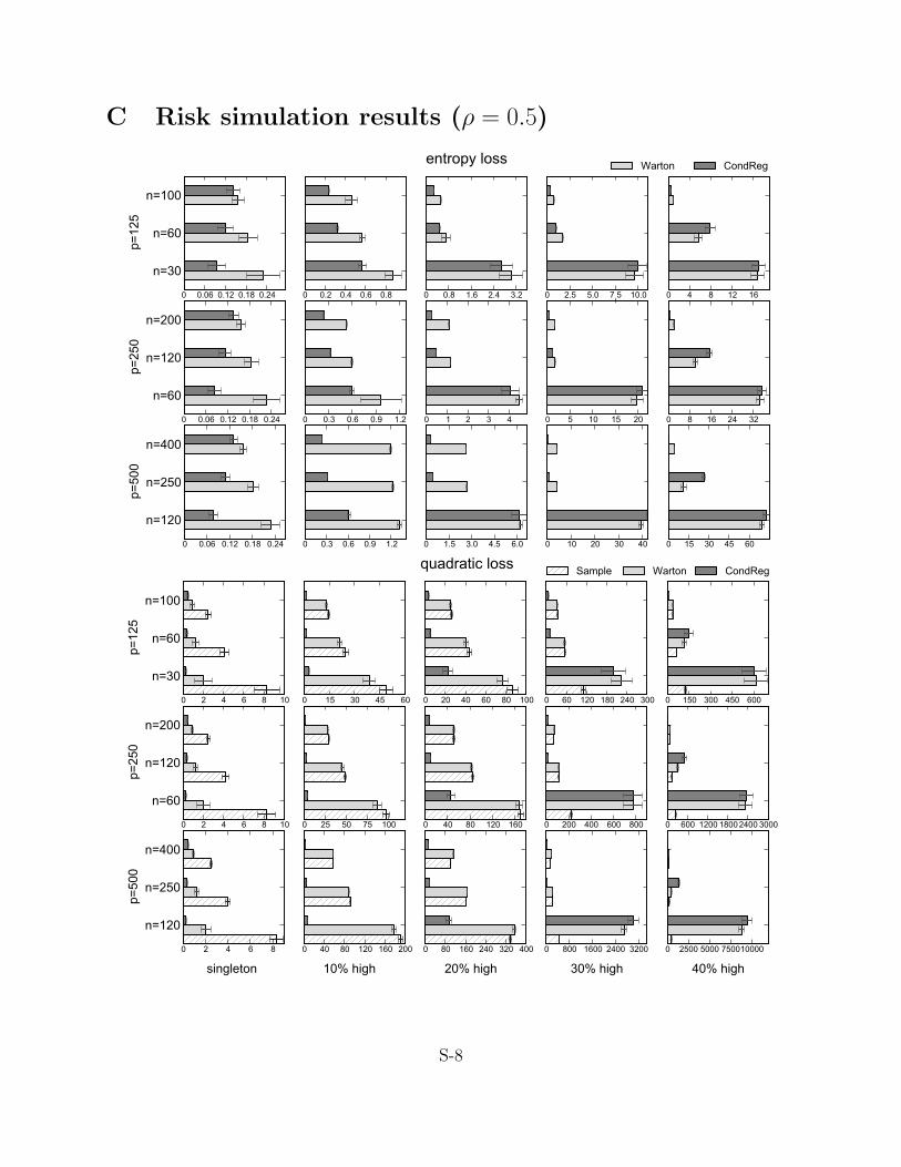
C Risk simulation results (ρ = 0.5)

singleton 10% high 20% high 30% high 40% high

S-8

Average risks (with error bars) over 1000 runs with respect to two loss functions ρ = 0.5. sample=samplecovariance matrix, Warton=linear shrinkage (Warton, 2008), CondReg=condition number regular-ization. Risks are normalized by the dimension (p).

D Empirical minimum variance rebalancing study (Sec-

tion 6.2)

D.1 List of the Dow Jones constituents

The Dow Jones stocks used in our numerical study and their market performance over the periodfrom February 18, 1994 to June 6, 2008. The return, risk and the Sharpe ratio (SR) are annualized.

index company ticker return [%] risk [%] SR1 3M Company MMM 12.04 10.74 0.252 Alcoa, Inc. AA 16.50 15.47 0.303 American Express AXP 17.52 14.61 0.354 American International Group, Inc. AIG 7.96 12.93 0.075 AT&T Inc. T 11.57 12.95 0.196 Bank of America BAC 11.57 13.14 0.197 The Boeing Company BA 13.03 13.81 0.238 Caterpillar Inc. CAT 18.53 14.26 0.399 Chevron Corporation CVX 15.86 10.53 0.42

10 Citigroup Inc. C 14.44 15.27 0.2511 The Coca-Cola Company KO 10.74 10.77 0.2012 E.I. du Pont de Nemours & Company DD 9.58 12.43 0.1313 Exxon Mobil Corporation XOM 16.58 10.46 0.4514 General Electric Company GE 13.47 12.04 0.2815 General Motors Corporation GM -1.24 15.85 -0.2016 The Hewlett-Packard Company HPQ 20.22 18.24 0.3517 The Home Depot HD 12.96 15.28 0.2018 Intel Corporation INTC 20.84 19.13 0.3519 International Business Machines Corp. IBM 20.99 13.86 0.4820 Johnson & Johnson JNJ 17.13 10.10 0.4921 JPMorgan Chase & Co. JPM 15.84 15.44 0.2922 McDonald’s Corporation MCD 14.05 12.05 0.3023 Merck & Co., Inc. MRK 12.86 12.87 0.2424 Microsoft Corporation MSFT 22.91 15.13 0.5025 Pfizer Inc. PFE 15.34 12.92 0.3226 The Procter & Gamble Company PG 15.25 11.06 0.3727 United Technologies Corporation UTX 18.93 12.37 0.4728 Verizon Communications Inc. VZ 9.93 12.38 0.1429 Wal-Mart Stores, Inc. WMT 14.86 13.16 0.3030 The Walt Disney Company DIS 10.08 14.05 0.13

S-9

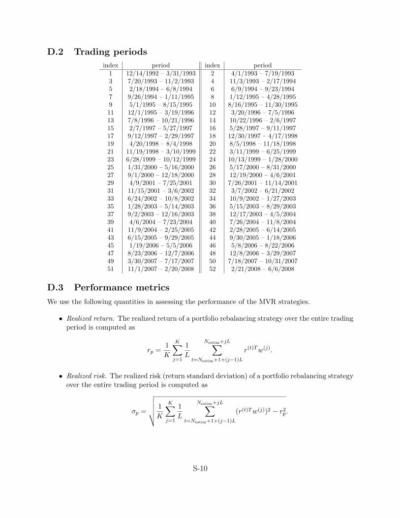
D.2 Trading periods

index period index period1 12/14/1992 – 3/31/1993 2 4/1/1993 – 7/19/19933 7/20/1993 – 11/2/1993 4 11/3/1993 – 2/17/19945 2/18/1994 – 6/8/1994 6 6/9/1994 – 9/23/19947 9/26/1994 – 1/11/1995 8 1/12/1995 – 4/28/19959 5/1/1995 – 8/15/1995 10 8/16/1995 – 11/30/199511 12/1/1995 – 3/19/1996 12 3/20/1996 – 7/5/199613 7/8/1996 – 10/21/1996 14 10/22/1996 – 2/6/199715 2/7/1997 – 5/27/1997 16 5/28/1997 – 9/11/199717 9/12/1997 – 2/29/1997 18 12/30/1997 – 4/17/199819 4/20/1998 – 8/4/1998 20 8/5/1998 – 11/18/199821 11/19/1998 – 3/10/1999 22 3/11/1999 – 6/25/199923 6/28/1999 – 10/12/1999 24 10/13/1999 – 1/28/200025 1/31/2000 – 5/16/2000 26 5/17/2000 – 8/31/200027 9/1/2000 – 12/18/2000 28 12/19/2000 – 4/6/200129 4/9/2001 – 7/25/2001 30 7/26/2001 – 11/14/200131 11/15/2001 – 3/6/2002 32 3/7/2002 – 6/21/200233 6/24/2002 – 10/8/2002 34 10/9/2002 – 1/27/200335 1/28/2003 – 5/14/2003 36 5/15/2003 – 8/29/200337 9/2/2003 – 12/16/2003 38 12/17/2003 – 4/5/200439 4/6/2004 – 7/23/2004 40 7/26/2004 – 11/8/200441 11/9/2004 – 2/25/2005 42 2/28/2005 – 6/14/200543 6/15/2005 – 9/29/2005 44 9/30/2005 – 1/18/200645 1/19/2006 – 5/5/2006 46 5/8/2006 – 8/22/200647 8/23/2006 – 12/7/2006 48 12/8/2006 – 3/29/200749 3/30/2007 – 7/17/2007 50 7/18/2007 – 10/31/200751 11/1/2007 – 2/20/2008 52 2/21/2008 – 6/6/2008

D.3 Performance metrics

We use the following quantities in assessing the performance of the MVR strategies.

• Realized return. The realized return of a portfolio rebalancing strategy over the entire tradingperiod is computed as

rp =1

K

K∑

j=1

1

L

Nestim+jL∑

t=Nestim+1+(j−1)L

r(t)Tw(j).

• Realized risk. The realized risk (return standard deviation) of a portfolio rebalancing strategyover the entire trading period is computed as

σp =

√√√√√ 1

K

K∑

j=1

1

L

Nestim+jL∑

t=Nestim+1+(j−1)L

(r(t)Tw(j))2 − r2p.

S-10

• Realized Sharpe ratio (SR). The realized Sharpe ratio, i.e., the ratio of the excess expectedreturn of a portfolio rebalancing strategy relative to the risk-free return rf is given by

SR =rp − rfσp

.

• Turnover. The turnover from the portfolio w(j) held at the start date of the jth holdingperiod [Nestim +1+ (j − 1)L,Nestim + jL] to the portfolio w(j−1) held at the previous periodis computed as

TO(j) =

p∑

i=1

∣∣∣∣∣∣w

(j)i −

Nestim+jL∏

t=Nestim+1+(j−1)L

r(t)i

w

(j−1)i

∣∣∣∣∣∣.

For the first period, we take w(0) = 0, i.e., the initial holdings of the assets are zero.

• Normalized wealth growth. Let w(j) = (w(j)1 , . . . , w

(j)n ) be the portfolio constructed by a

rebalancing strategy held over the jth holding period [Nestim + 1 + (j − 1)L,Nestim + jL].When the initial budget is normalized to one, the normalized wealth grows according to therecursion

W (t) =

W (t− 1)(1 +

∑pi=1witr

(t)i ), t 6∈ Nestim + jL | j = 1, . . . ,K,

W (t− 1)(1 +∑p

i=1witr(t)i )− TC(j), t = Nestim + jL,

for t = Nestim, . . . , Nestim +KL, with the initial wealth W (Nestim) = 1. Here

wit =

w(1)i , t = Nestim + 1, . . . , Nestim + L,...

w(K)i , t = Nestim + 1 + (K − 1)L, . . . , Nestim +KL.

and

TC(j) =

p∑

i=1

ηi

∣∣∣∣∣∣w

(j)i −

Nestim+jL∏

t=Nestim+1+(j−1)L

r(t)i

w

(j−1)i

∣∣∣∣∣∣

is the transaction cost due to the rebalancing if the cost to buy or sell one share of stock i isηi.

• Size of the short side. The size of the short side of a portfolio rebalancing strategy over theentire trading period is computed as

rp =1

K

K∑

j=1

(p∑

i=1

|min(w(j)i , 0)|/

p∑

i=1

|w(j)i |).

D.4 Minimum variance portfolio theoretic performance metrics

Realized utility, realized return, and realized risk based on different regularization schemes for co-variance matrices are reported. sample=sample covariance matrix, LW=linear shrinkage (Ledoit and

S-11

Wolf, 2004), Warton=linear shrinkage (Warton, 2008), condreg=condition number regularization.Each entry is the mean (standard deviation) of the corresponding metric over the trading period

(48 holding periods) from February 1994 through June 2008. The standard deviations are computedin a heteroskedasticity-and-autocorrelation consistent manner discussed by Ledoit and Wolf (2008,Sec. 3.1.). For comparison, the performance metrics of the S&P 500 index for the same period arereported at the end of the table. All values are annualized.

covarianceregularization scheme

return [%] risk [%] SR

Nestim = 15sample – – –

LW 12.12 (3.69) 14.38 (0.69) 0.50 (0.26)Warton 12.21 (3.71) 14.28 (0.68) 0.50 (0.26)condreg 14.49 (4.01) 16.07 (0.94) 0.59 (0.25)

condreg - LW 2.37 (5.45) 1.69 (1.17) 0.10 (0.36)condreg - Warton 2.28 (5.47) 1.79 (1.16) 0.09 (0.37)

Nestim = 30sample 145.91 (114.74) 851.07 (257.28) 0.17 (0.14)

LW 11.82 (3.72) 14.27 (0.65) 0.48 (0.26)Warton 12.1 (3.68) 14.06 (0.69) 0.51 (0.27)condreg 14.32 (4.00) 15.92 (0.91) 0.59 (0.26)

condreg - LW 2.51 (5.46) 1.65 (1.12) 0.11 (0.37)condreg - Warton 2.16 (5.43) 1.85 (1.14) 0.08 (0.37)

Nestim = 45sample 9.52 (5.62) 21.15 (0.74) 0.21 (0.26)

LW 12.21 (3.65) 14.04 (0.72) 0.51 (0.26)Warton 12.62 (3.60) 13.85 (0.76) 0.55 (0.26)condreg 14.53 (3.93) 15.63 (0.87) 0.61 (0.26)

condreg - LW 2.33 (5.36) 1.60 (1.13) 0.10 (0.37)condreg - Warton 1.91 (5.33) 1.79 (1.16) 0.06 (0.37)

Nestim = 60sample 9.32 (4.29) 17.52 (0.70) 0.25 (0.25)

LW 11.55 (3.55) 13.94 (0.74) 0.47 (0.26)Warton 12.15 (3.55) 13.78 (0.77) 0.52 (0.26)condreg 14.13 (3.91) 15.65 (0.90) 0.58 (0.25)

condreg - LW 2.58 (5.28) 1.71 (1.17) 0.11 (0.36)condreg - Warton 1.98 (5.28) 1.87 (1.18) 0.06 (0.37)

S&P500– 8.71 (3.84) 16.04 (0.94) 0.23 (0.24)

D.5 Turnover

Turnover for various estimation horizon sizes over the trading period from February 18, 1994through June 6, 2008. sample=sample covariance matrix, LW=linear shrinkage (Ledoit and Wolf,2004), Warton=linear shrinkage (Warton, 2008), condreg=condition number regularization.

S-12

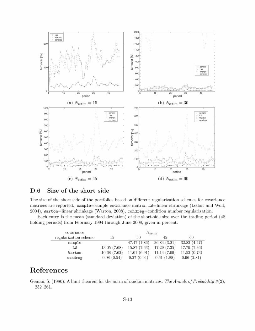
5 15 25 35 450

100

200

period

turn

ove

r [%

]

LWWartoncondreg

5 15 25 35 450

200

400

600

800

1000

1200

1400

1600

1800

2000

period

turn

ove

r [%

]

sample

LW

Wartoncondreg

(a) Nestim = 15 (b) Nestim = 30

5 15 25 35 450

100

200

300

400

500

600

700

800

900

1000

period

turn

ove

r [%

]

sample

LWWarton

condreg

5 15 25 35 450

100

200

300

400

500

600

700

period

turn

ove

r [%

]

sample

LWWartoncondreg

(c) Nestim = 45 (d) Nestim = 60

D.6 Size of the short side

The size of the short side of the portfolios based on different regularization schemes for covariancematrices are reported. sample=sample covariance matrix, LW=linear shrinkage (Ledoit and Wolf,2004), Warton=linear shrinkage (Warton, 2008), condreg=condition number regularization.

Each entry is the mean (standard deviation) of the short-side size over the trading period (48holding periods) from February 1994 through June 2008, given in percent.

covarianceregularization scheme

Nestim

15 30 45 60sample – 47.47 (1.86) 36.84 (3.21) 32.83 (4.47)

LW 13.05 (7.68) 15.87 (7.63) 17.29 (7.35) 17.79 (7.36)Warton 10.68 (7.62) 11.01 (6.91) 11.14 (7.09) 11.53 (0.73)condreg 0.08 (0.54) 0.27 (0.94) 0.61 (1.88) 0.96 (2.81)

References

Geman, S. (1980). A limit theorem for the norm of random matrices. The Annals of Probability 8 (2),252–261.

S-13

Ledoit, O. and M. Wolf (2004). A well-conditioned estimator for large-dimensional covariancematrices. Journal of Multivariate Analysis 88, 365–411.

Ledoit, O. and M. Wolf (2008, December). Robust performance hypothesis testing with the sharperatio. Journal of Empirical Finance 15 (5), 850–859.

Silverstein, J. W. (1985). The smallest eigenvalue of a large dimensional wishart matrix. TheAnnals of Probability 13 (4), 1364–1368.

Warton, D. I. (2008). Penalized Normal Likelihood and Ridge Regularization of Correlation andCovariance Matrices. Journal of the American Statistical Association 103 (481), 340–349.

Yang, R. and J. O. Berger (1994). Estimation of a covariance matrix using the reference prior. TheAnnals of Statistics 22 (3), 1195–1211.

S-14