cone-based electrical resistivity tomographyhaber/pubs/pidlisecky_knight_haber_2006.pdf ·...

C

A

cStlbosenhrcbe

p

m

GEOPHYSICS, VOL. 71, NO. 4 �JULY-AUGUST 2006�; P. G157–G167, 13 FIGS., 2 TABLES.10.1190/1.2213205

one-based electrical resistivity tomography

dam Pidlisecky1, Rosemary Knight1, and Eldad Haber2

ABSTRACT

Determining the 3D spatial distribution of subsurface proper-ties is a challenging, but critical, part of managing the cleanup ofcontaminated sites. We have developed a minimally invasivetechnology that can provide information about the 3D distribu-tion of electrical conductivity. The technique, cone-based elec-trical resistivity tomography �C-bert�, integrates resistivity to-mography with cone-penetration testing. Permanent currentelectrodes are emplaced in the subsurface and used to inject cur-rent into the subsurface region of interest. The resultant potentialfields are measured using a surface reference electrode and anelectrode mounted on a cone penetrometer. The standard suite ofcone penetration measurements, including high-resolution resis-tivity logs, are also obtained and are an integral part of the C-bertmethod. C-bert data are inverted using an inexact Gauss-Newtonalgorithm to produce a 3D electrical conductivity map. A major

challenge with the inversion is the large local perturbationaround the measurement location, due to the highly conductivecone. As the cone is small with respect to the total model space,explicit modeling of the cone is cost prohibitive. We have devel-oped a rapid method for solving the forward model which uses it-eratively determined boundary conditions �IDBC�. This allowsus to generate a computationally feasible, preinversion correc-tion for the cone perturbation. We assessed C-bert by performinga field test to image the conductivity structure of the Kidd 2 sitenear Vancouver, British Columbia.Atotal of nine permanent cur-rent electrodes were emplaced and five C-bert data sets were ob-tained, resulting in 6516 data points. These data were inverted toobtain a 3D conductivity image of the subsurface. Furthermore,we demonstrated, using a synthetic experiment, that C-bert canyield high quality electrical conductivity images in challengingfield situations. We conclude that C-bert is a promising new im-aging technique.

r2ta2

qtcawhtnem

ved Novding, S

Mathem

INTRODUCTION

One of the main challenges in the cleanup and management of aontaminated site is developing an accurate model of the subsurface.uch a model ideally contains information about the location of con-

aminants, and information about the subsurface properties control-ing the long-term fate and transport of the contaminants. Borehole-ased electrical resistivity tomography �ERT� is a geophysical meth-d that increasingly is being used to assist in the development of sub-urface models. ERT involves injecting current through a pair oflectrodes in one borehole, and measuring the resulting potentials atumerous �tens to hundreds of� electrodes located in the same bore-ole, and in different boreholes. The measurements yield values ofesistance that can be inverted to determine the subsurface electricalonductivity structure. The electrical conductivity structure haseen used, for example, to infer the presence of a contaminant, withlectrical conductivity different from that of the background envi-

Manuscript received by the Editor June 29, 2005; revised manuscript recei1Stanford University, Department of Geophysics, 2215 Mitchell Buil

angea.stanford.edu.2Emory University, Department of Mathematics and Computer Science,

athcs.emory.edu.© 2006 Society of Exploration Geophysicists.All rights reserved.

G157

onment, �e.g., Daily and Ramirez, 1995; LaBrecque and Yang,001� and to obtain information about potential flow paths of con-aminants by imaging the movement of conductive tracers �Slater etl., 2000; Versteeg et al., 2000; Kemna et al., 2002; Slater et al.,002; Singha and Gorelick, 2005�.

A critical problem with the use of borehole-based ERT is the re-uirement of boreholes. Boreholes are not desirable at many con-aminated sites due to the fact that installation is expensive, timeonsuming, and risks the exposure of workers to contaminants. Inddition, there is potential for mobilizing contaminants by creating,ith the boreholes, new pathways in the subsurface. These issuesave motivated us to develop an ERT system that does not requirehe use of boreholes, but uses a cone penetrometer to position a smallumber of subsurface current electrodes around the region of inter-st and to make potential field measurements between an electrodeounted on the cone and a surface reference electrode.

ember 30, 2005; published online July 31, 2006.tanford, California 94305. E-mail: [email protected]; rknight@

atics and Science Building E414, Atlanta, Georgia 30322. E-mail: haber@

tcamitn1scmcnrav�ba

itsotctfb

i�ems�ta

mtmmaRd

covEs�osfdt

tpidt

smtathlsJ2

dFsaF

Fr

Fba

G158 Pidlisecky et al.

The cone penetrometer is a testing tool that was developed by geo-echnical engineers for obtaining high-resolution depth logs of me-hanical soil properties. A cone penetrometer, commonly referred tos a cone, is a 36-mm diameter steel rod, �1 m long, with sensorsounted close to a cone-shaped tip. Cone penetration testing �CPT�,

.e., using the cone for subsurface characterization, is a techniquehat is now widely used in the environmental and geotechnical engi-eering community �Campanella and Weemees, 1990; Daniel et al.,999�. The technique is classified as minimally invasive, because in-tead of drilling a borehole to make subsurface measurements, aone is pushed into unconsolidated materials using hydraulic ramsounted on a large truck, referred to as the cone truck. While the

one is being pushed, measurements are made with the sensors in aear-continuous fashion, with typical sampling every 2.5 cm. Toeach the measurement depth of interest, 1-m sections of steel rod aredded to the end of the cone. The maximum depth of investigationaries with the geologic environment, but is generally limited to100 m. CPT is an efficient, relatively inexpensive alternative to

orehole installation and works extremely well in areas of alluvialnd deltaic deposits consisting of clays, silts, or sands.

The standard cone penetrometer, as most commonly configured,s shown schematically in Figure 1a. This standard cone measureshree separate ground properties: tip penetration resistance, frictionleeve resistance, and induced pore pressure, all of which are used tobtain information about subsurface stratigraphy. The accelerome-ers can be calibrated to function as deviation sensors so that the conean be accurately located. However, in standard cone penetrationesting the accelerometers are rarely used for this purpose, and there-ore, the uncertainties associated with these measurements have noteen well established.

Of use for identifying zones of anomalous electrical conductivitys the method referred to as resistivity cone penetrometer testingRCPT�, which uses a resistivity module containing two pairs of ringlectrodes. What is referred to as the resistivity cone is shown sche-atically in Figure 1b and includes the resistivity module and the

tandard cone. To make a measurement, a high-frequency�1000 Hz� AC current is injected into one pair of electrodes, andhe voltage is measured across the same pair of electrodes �Lunne etl., 1997�. Figure 1b shows the two electrode pairs; the measure-

igure 1. Schematics of �a� a standard cone penetrometer and �b� aesistivity cone.

ents are made using each electrode pair. The separation distance ofhe electrodes, along with the resistivity of the surrounding sedi-

ents, determines the volume sampled by the measurement. Theodule is 36.6 mm in diameter, which is slightly larger than the di-

meter of the standard cone to ensure good soil-electrode coupling.CPT yields a high-resolution resistivity log in addition to the stan-ard suite of cone data.

Recent work has highlighted the advantage of coupling geophysi-al imaging techniques with CPT. Narbutovskih et al. �1997� dem-nstrated the benefit of using CPT technology to emplace permanentertical electrode arrays to monitor infiltration experiments usingRT. Their design proved successful, and showed the advantages inpeed, cost, and safety over borehole-based ERT. Jarvis and Knight2000, 2002� used a vertical seismic profile, obtained using acceler-meters mounted on a cone, to constrain the inversion of 2D seismichear-wave reflection data, thus improving the quality of the subsur-ace velocity model. Motivated by these previous studies, we haveeveloped an acquisition system that combines ERT and CPT so aso gain the benefits realized by these studies.

In this paper, we present our new cone-based ERT �C-bert� sys-em. We describe in detail a successful field test of this new ap-roach, covering both the field procedures and the data processing/nterpretation algorithms. We conclude with a synthetic example toemonstrate the potential of C-bert as a new way to obtain conduc-ivity images of the subsurface.

DESCRIPTION OF FIELD SITE

The field experiment was conducted at the BC Hydro Kidd 2 re-earch site in Richmond, British Columbia, Canada. The site is im-ediately adjacent to the Fraser River and has a zone of saltwater in-

rusion, extending well into the site �Neilson-Welch 1999�. Kidd 2 isvery well-documented site, having been the focus of several geo-

echnical, geophysical, and hydrogeologic studies. Work on the siteas included multiple cone penetrometer tests, multiple hydrogeo-ogic well installations, various geophysical surveys, and the analy-is of numerous core samples �Hofmann, 1997; Hunter et al., 1998;arvis et al., 1999; Neilson-Welch, 1999; Neilson-Welch and Smith,001; Jarvis and Knight, 2000, 2002�.

The Kidd 2 site is composed of Holocene sediments depositeduring the progradation of the Fraser River �Clague et al., 1983�.igure 2 is a cross section through the area around the Kidd 2 site,howing the five hydrostratigraphic units defined by Neilson-Welchnd Smith �2001�; these units are described in Table 1.Also shown inigure 2 is the approximate extent of the saltwater intrusion. Imag-

igure 2. A cross section of the Kidd 2 site, with the approximateoundary of the saltwater intrusion overlaid �after Neilson-Welchnd Smith, 2001�.

io

C�lcwtRm�mosemcetc

D

aac

mgt�pwwr

D

atrtTdw�safssfm

tatuiot

qsp

D

top

TW

d

FTtp

Cone-based electrical resistivity tomography G159

ng the conductivity structure to a depth of 30 m was defined as thebjective of our C-bert field test.

KIDD 2 C-BERT EXPERIMENT

Figure 3 is a schematic that illustrates the basic components of the-bert system used at the field site. The survey area was 35 � 30 m

in the north-south and east-west directions, respectively�. At nineocations on the grid, we used a cone truck to emplace permanenturrent electrodes in the subsurface. Once the current electrodesere in place, we pushed a resistivity cone into the ground and began

he process referred to as C-bert. We acquired data in the standardCPT mode, using the outer pair of electrodes on the resistivityodule to obtain a 1D resistivity profile. At regular depth intervals

every 1–2 m�, the cone was stopped and resistivity tomographyeasurements were made. To do this, current was injected into a pair

f the permanent current electrodes. The potential drop was mea-ured between a surface reference potential electrode, and the innerlectrodes on the resistivity module �i.e., on the cone�. This form ofeasurement was repeated for all independent current pairs. The

one was then pushed to the next interval, and the procedure repeat-d. This continued until the cone reached approximately 30 m. Theruck was then moved, and the experiment repeated at a different lo-ation. Below, we describe in detail this field experiment.

escription of cone truck

We used the cone truck from the Department of Civil Engineeringt the University of British Columbia �UBC�. The UBC cone truck isself-contained laboratory with all of the equipment needed for thealibration and deployment of the resistivity cone.

In an effort to reduce sources of electrical noise during C-berteasurements, the cone truck was electrically isolated from the

round and the cone rods. The hydraulic jack pads, which allow theruck to be lifted and leveled, are large steel plates, approximately 1

2 � 0.5 m. In order to isolate the truck from the ground, welaced 2 mm thick PVC mats under the jack pads. Another concernas the two metal guides that keep the cone rod centered and alignedith the hydraulic rams. In order to isolate the truck from the cone

ods plastic guides were used.

able 1. Kidd 2 Hydrostratigraphic units (after Neilson-elch and Smith, 2001).

Unitesignation

Approximatedepth �m� Description

1 1–3.5 Clayey silt: clayey silt with tracefine sand laminations

2 3.5–9 Silty sand: fine- and medium-grainedsand with interbeds of clayey silt,sandy silt, and fine sand

3 9–12 Fine and medium sand: includesinterbeds of silt and finesand

4 12–22 Medium sand: uniform medium sandwith trace interbedsof silts

5 �22 Silty clay: includes thin laminationsof silt

escription of the resistivity cone

The resistivity cone used in our study contained a standard conend a resistivity module built by UBC. There are four brass ring elec-rodes on the module, arranged as two electrode pairs, one pair sepa-ated by �10 mm, the other by �150 mm. We used only the elec-rode pair separated by 150 mm to make the RCPT measurements.his electrode pair was calibrated using a technique similar to thatescribed in Campanella and Weemees �1990�. The resistivity coneas immersed in a 2 � 2 � 1.5 m water tank. Sodium chloride

NaCl� was added to the tank; the resistivity of the water was mea-ured with a conductivity probe; and the voltage was measuredcross the cone electrodes. This procedure was repeated �20 timesor different concentrations of NaCl. We observed a linear relation-hip between the cone voltage measurements and the probe-mea-ured resistivity of the water, allowing us to define the calibrationactor needed to obtain resistivity values from our cone measure-ents.Making subsurface ERT measurements requires a potential elec-

rode below the surface.Akey part of the C-bert concept is the use ofn electrode, pushed into the subsurface on the resistivity cone, ashe subsurface potential electrode. We modified the resistivity mod-le on the cone so that the inner electrode pair functioned as a single,solated electrode. The C-bert system thus included the use of theuter electrodes on the resistivity module for resistivity logging, andhe use of the inner electrodes for ERT measurements.

In addition to the two forms of resistance measurements, we ac-uired the standard suite of cone measurements. Once at the fieldite, the sensors in the standard cone were calibrated and the poreressure sensor saturated as described in Lunne et al. �1997�.

esign and emplacement of permanent electrodes

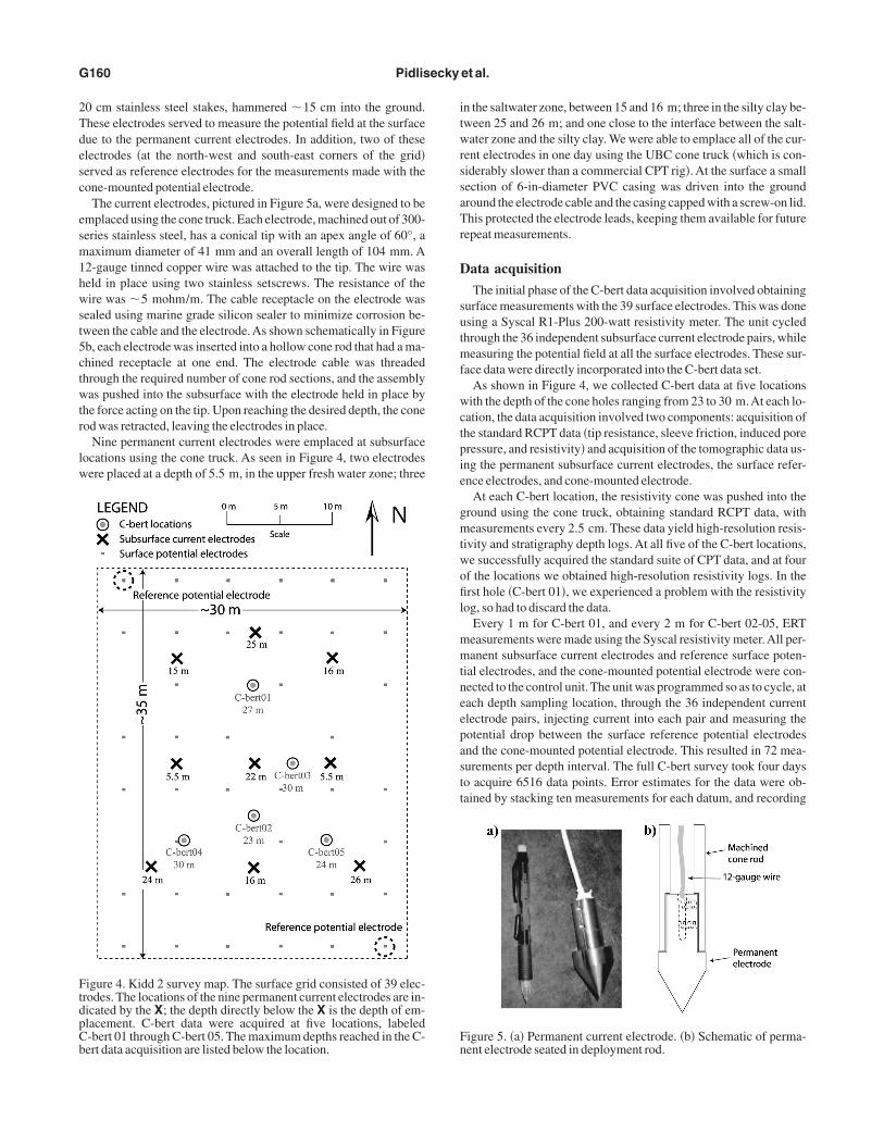
Figure 4 shows the plan of the survey grid, 35 � 30 m, coveringhe Kidd 2 site. On this plan view are shown the locations and depthsf all the permanent electrodes. Also shown are the locations of 39otential electrodes placed at the surface. These electrodes were

igure 3. Schematic of a cone-based resistivity tomography system.he current electrodes are permanently emplaced prior to C-bert

esting. Potential measurements are made using the cone-mountedotential electrode and can thus be made anywhere in the volume.

2Tdesc

esm1hwst5ctwtr

lw

itwrssaTr

D

sutmf

wctpie

gmtwofil

mmtneepastt

FtdpCb

Fn


0 cm stainless steel stakes, hammered �15 cm into the ground.hese electrodes served to measure the potential field at the surfaceue to the permanent current electrodes. In addition, two of theselectrodes �at the north-west and south-east corners of the grid�erved as reference electrodes for the measurements made with theone-mounted potential electrode.

The current electrodes, pictured in Figure 5a, were designed to bemplaced using the cone truck. Each electrode, machined out of 300-eries stainless steel, has a conical tip with an apex angle of 60°, aaximum diameter of 41 mm and an overall length of 104 mm. A

2-gauge tinned copper wire was attached to the tip. The wire waseld in place using two stainless setscrews. The resistance of theire was �5 mohm/m. The cable receptacle on the electrode was

ealed using marine grade silicon sealer to minimize corrosion be-ween the cable and the electrode. As shown schematically in Figureb, each electrode was inserted into a hollow cone rod that had a ma-hined receptacle at one end. The electrode cable was threadedhrough the required number of cone rod sections, and the assemblyas pushed into the subsurface with the electrode held in place by

he force acting on the tip. Upon reaching the desired depth, the coneod was retracted, leaving the electrodes in place.

Nine permanent current electrodes were emplaced at subsurfaceocations using the cone truck. As seen in Figure 4, two electrodesere placed at a depth of 5.5 m, in the upper fresh water zone; three

igure 4. Kidd 2 survey map. The surface grid consisted of 39 elec-rodes. The locations of the nine permanent current electrodes are in-icated by the X; the depth directly below the X is the depth of em-lacement. C-bert data were acquired at five locations, labeled-bert 01 through C-bert 05. The maximum depths reached in the C-ert data acquisition are listed below the location.

n the saltwater zone, between 15 and 16 m; three in the silty clay be-ween 25 and 26 m; and one close to the interface between the salt-ater zone and the silty clay. We were able to emplace all of the cur-

ent electrodes in one day using the UBC cone truck �which is con-iderably slower than a commercial CPT rig�. At the surface a smallection of 6-in-diameter PVC casing was driven into the groundround the electrode cable and the casing capped with a screw-on lid.his protected the electrode leads, keeping them available for future

epeat measurements.

ata acquisition

The initial phase of the C-bert data acquisition involved obtainingurface measurements with the 39 surface electrodes. This was donesing a Syscal R1-Plus 200-watt resistivity meter. The unit cycledhrough the 36 independent subsurface current electrode pairs, while

easuring the potential field at all the surface electrodes. These sur-ace data were directly incorporated into the C-bert data set.

As shown in Figure 4, we collected C-bert data at five locationsith the depth of the cone holes ranging from 23 to 30 m.At each lo-

ation, the data acquisition involved two components: acquisition ofhe standard RCPT data �tip resistance, sleeve friction, induced poreressure, and resistivity� and acquisition of the tomographic data us-ng the permanent subsurface current electrodes, the surface refer-nce electrodes, and cone-mounted electrode.

At each C-bert location, the resistivity cone was pushed into theround using the cone truck, obtaining standard RCPT data, witheasurements every 2.5 cm. These data yield high-resolution resis-

ivity and stratigraphy depth logs. At all five of the C-bert locations,e successfully acquired the standard suite of CPT data, and at fourf the locations we obtained high-resolution resistivity logs. In therst hole �C-bert 01�, we experienced a problem with the resistivity

og, so had to discard the data.Every 1 m for C-bert 01, and every 2 m for C-bert 02-05, ERTeasurements were made using the Syscal resistivity meter.All per-anent subsurface current electrodes and reference surface poten-

ial electrodes, and the cone-mounted potential electrode were con-ected to the control unit. The unit was programmed so as to cycle, atach depth sampling location, through the 36 independent currentlectrode pairs, injecting current into each pair and measuring theotential drop between the surface reference potential electrodesnd the cone-mounted potential electrode. This resulted in 72 mea-urements per depth interval. The full C-bert survey took four dayso acquire 6516 data points. Error estimates for the data were ob-ained by stacking ten measurements for each datum, and recording

igure 5. �a� Permanent current electrode. �b� Schematic of perma-ent electrode seated in deployment rod.

tttrcpttawi

R

sbmorpttv

tfaslsMmtBwsFsthtom

E

sttwd

Ettt�cacay

Hfettdtdfawaoaufi

Tt

C

C

C

C

C Fa


he standard deviation of these measurements. Typically, in resistivi-y experiments reciprocal measurements are used for determininghe noise level. Reciprocal measurements involve switching the cur-ent and potential measurement pairs for each location. The recipro-al measurements should yield identical results, and any variationrovides quantification of error �Binley et al., 2002�. However, withhe C-bert acquisition system, we are unable to inject currenthrough the cone mounted electrode, because the wiring and circuitsre not designed to accommodate large amounts of current, and thus,e could not obtain reciprocals. Table 2 is a compilation of the start-

ng depths, depth intervals, and finishing depths of the survey.

FIELD RESULTS AND INTERPRETATION

esistivity cone data

Inversion of ERT is a highly nonlinear optimization problem. Asuch, an accurate starting model greatly increases the rate and proba-ility of convergence of the inversion. Furthermore, this startingodel is often used as the reference model in the regularization term

f the inversion, and thus it will greatly affect the appearance of theesulting inversion. The suite of RCPT data, which is acquired asart of the C-bert experiment, provides valuable information abouthe subsurface, that can be used to build a good starting model. Fur-hermore, the resistivity data can be used as constraints within the in-ersion.

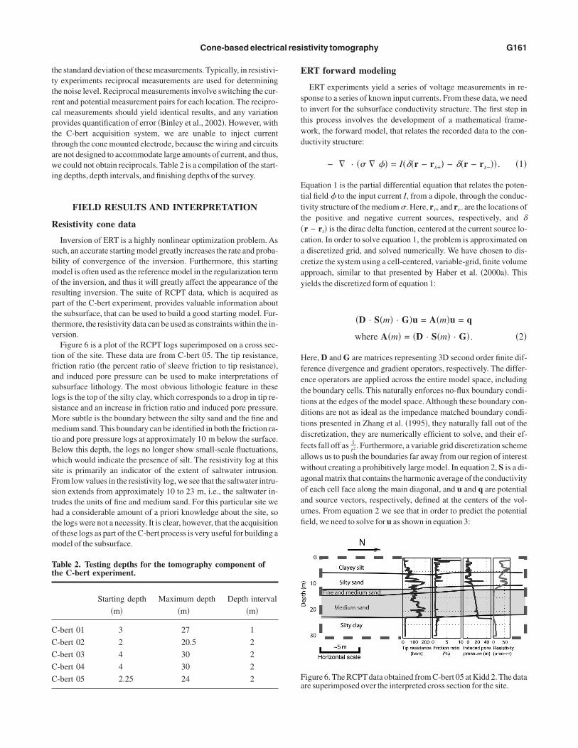
Figure 6 is a plot of the RCPT logs superimposed on a cross sec-ion of the site. These data are from C-bert 05. The tip resistance,riction ratio �the percent ratio of sleeve friction to tip resistance�,nd induced pore pressure can be used to make interpretations ofubsurface lithology. The most obvious lithologic feature in theseogs is the top of the silty clay, which corresponds to a drop in tip re-istance and an increase in friction ratio and induced pore pressure.

ore subtle is the boundary between the silty sand and the fine andedium sand. This boundary can be identified in both the friction ra-

io and pore pressure logs at approximately 10 m below the surface.elow this depth, the logs no longer show small-scale fluctuations,hich would indicate the presence of silt. The resistivity log at this

ite is primarily an indicator of the extent of saltwater intrusion.rom low values in the resistivity log, we see that the saltwater intru-ion extends from approximately 10 to 23 m, i.e., the saltwater in-rudes the units of fine and medium sand. For this particular site wead a considerable amount of a priori knowledge about the site, sohe logs were not a necessity. It is clear, however, that the acquisitionf these logs as part of the C-bert process is very useful for building aodel of the subsurface.

able 2. Testing depths for the tomography component ofhe C-bert experiment.

Starting depth Maximum depth Depth interval

�m� �m� �m�

-bert 01 3 27 1

-bert 02 2 20.5 2

-bert 03 4 30 2

-bert 04 4 30 2

-bert 05 2.25 24 2

RT forward modeling

ERT experiments yield a series of voltage measurements in re-ponse to a series of known input currents. From these data, we needo invert for the subsurface conductivity structure. The first step inhis process involves the development of a mathematical frame-ork, the forward model, that relates the recorded data to the con-uctivity structure:

− � · �� = I��r − rs+� − ��r − rs−�� . �1�

quation 1 is the partial differential equation that relates the poten-ial field � to the input current I, from a dipole, through the conduc-ivity structure of the medium �. Here, rs+ and rs− are the locations ofhe positive and negative current sources, respectively, and �r − rs� is the dirac delta function, centered at the current source lo-ation. In order to solve equation 1, the problem is approximated ondiscretized grid, and solved numerically. We have chosen to dis-

retize the system using a cell-centered, variable-grid, finite volumepproach, similar to that presented by Haber et al. �2000a�. Thisields the discretized form of equation 1:

�D · S�m� · G�u = A�m�u = q

where A�m� = �D · S�m� · G� . �2�

ere, D and G are matrices representing 3D second order finite dif-erence divergence and gradient operators, respectively. The differ-nce operators are applied across the entire model space, includinghe boundary cells. This naturally enforces no-flux boundary condi-ions at the edges of the model space. Although these boundary con-itions are not as ideal as the impedance matched boundary condi-ions presented in Zhang et al. �1995�, they naturally fall out of theiscretization, they are numerically efficient to solve, and their ef-ects fall off as 1

r2 . Furthermore, a variable grid discretization schemellows us to push the boundaries far away from our region of interestithout creating a prohibitively large model. In equation 2, S is a di-

gonal matrix that contains the harmonic average of the conductivityf each cell face along the main diagonal, and u and q are potentialnd source vectors, respectively, defined at the centers of the vol-mes. From equation 2 we see that in order to predict the potentialeld, we need to solve for u as shown in equation 3:

igure 6. The RCPT data obtained from C-bert 05 at Kidd 2. The datare superimposed over the interpreted cross section for the site.

Tc

cettg

E

sj

wetttmmas

e

wtmpdtnpba

moetf

wf

waftft

wcs�mpp

123

Wpttwt

Cctptt

acas

weltAgpdtohtscTi


u = A�m�−1q . �3�

he operator matrix A is sparse and banded; therefore, equation 3an be rapidly solved using preconditioned iterative methods.

For this work we used an incomplete LU decomposition for pre-onditioning. This is an expensive preconditioner to calculate; how-ver, as A remains the same for all our source terms, we can amortizehe cost over all the source vectors. The solution of equation 3 washen iteratively determined, for each source vector, using a biconju-ate stabilized gradient �Bicgstab� algorithm �Saad 1996�.

RT inversion

For this work, we chose to use an inexact Gauss-Newton inver-ion routine, similar to that described in Haber et al. �2000b�. The ob-ective function that we wish to minimize is the following:

minm�1

2�Wd�Qu − dobs��2 +

�

2�Wm�m − mref��2� , �4�

here Wd is the data weighting matrix; Q is a linear interpolation op-rator that projects the potentials u determined using equation 3 tohe corresponding locations where data were acquired; dobs is a vec-or containing the observed data;, Wm is a model regularization ma-rix; � is the regularization parameter that balances the effect of data

isfit and model regularization during the minimization; m is ourodel at a given iteration, where the model parameters are ln��;

nd mref our reference model, and in the case of the Kidd 2 data, ourtarting model, defined from our resistivity logs.

For the field data described here Wd is a matrix that contains thestimate of the absolute error along the main diagonal as follows:

diag�Wd� =1

�dobs� · SD�dobs�, �5�

here SD�dobs� is the standard deviation of the observed data, ob-ained from stacking measurements in the field. The regularization

atrix Wm is an anisotropic first derivative operator. This operatorromotes various levels of flatness in the x, y, and z directions. Theiagonal of Wm contains the relative weights of each model parame-er, in particular it contains weights that penalize model structureear our current electrode locations. For our work, the regularizationarameter � was set to at an initial value and progressively decreasedy a factor of 10 whenever the objective function was not reduced byt least 10% between iterations.

Using the inexact Gauss-Newton method we define a startingodel, mi �in this case mref�, that we hope is near the local minimum

f equation 4. The expressions under the norms in equation 4 are lin-arized about this model, and we calculate a small model update �mo obtain our new solution. The update is applied to the new model asollows:

mi+1 = mi + ��m , �6�

here mi+1 is the new model, and � is a line search parameter. Theorm of the Gauss-Newton update is as follows:

�7�

here J is the Jacobian or sensitivity matrix � �d�m�. The matrix H is an

pproximation to the Hessian, while g is the gradient of our objectiveunction. It should be noted that J is a very large, dense matrix, andhus, from a computational point of view, we want to avoid explicitlyorming the matrix. However, it was shown in Haber et al. �2000b�hat J has the form

J = QA−1B , �8�

here B =��A�m�u�

�m . The matrices B and Q are sparse matrices. Wean see from equation 8 that we can calculate the product of the sen-itivity matrix and a vector �or its adjoint� by solving the forwarddescribed by equation 3� or adjoint problems along with two matrixultiplications. Because of this, we do not compute the Hessian ex-

licitly but instead perform a series of matrix-vector products. Therocedure for calculating J is as follows:

� Calculate w = B · v� Solve x = A�m�−1y using Bicgstab.� Calculate J · v = Q · x

ith this in mind, a natural way to solve equation 7 is by using thereconditioned conjugate gradient method �PCG�, where only ma-rix-vector products need to be computed. Note that each PCG itera-ion involves one forward solve and one adjoint solve. In addition,e have to perform one forward solve and one adjoint solve in order

o evaluate the gradient g �Haber et al., 2000b�.The data from the RCPT logs, obtained coincidently with the

-bert data, were included as constraints in the inversion. These dataan be added to the inversion by either setting the values of the cellso their known value or as softer information by using them in theenalty function Wm. For our work, we chose to include these data inhe penalty function; this is done by applying a large model weight athe RCPT locations and applying no model update at these locations.

After each model update, the objective function is reevaluated,nd the line search parameter � is determined to ensure sufficient de-rease of the objective function. The line search parameter � starts atfixed value �usually one� and is reduced until the objective functionatisfies theArmijo inequality:

��mi+1� = ��mi + ��m� ��mi� + c1� � ��mi�T�m ,

�9�

here c1 is a constant, that in practice takes a very small value, forxample 10−4 and � is the value of the objective function. After theine search, if equation 4 has been minimized to the desired tolerancehe inversion is terminated, otherwise another iteration is performed.dditionally, we use the gradient term g in equation 7 as a conver-ence indicator; once the gradient g becomes small, no further im-rovements can be obtained with additional iterations. For our fieldata, we had an excellent starting model from the RCPT logs, andhus convergence was usually obtained within three to five iterationsf equation 7. This highlights another advantage of C-bert: we haveigh-resolution logs to construct a good starting model. We note thathese inversions results are nonunique. By combining an informedtarting model, an informed reference model and resistivity logs asonstraints, we substantially reduce the pool of plausible solutions.his yields better results than using any of this a priori information

ndependently.

T

clsfrtwdftwc1gptfrstv

dlattddsavpsccoasagsawrzefitrpfmts

1

maghtshto

smeesto

trnd

Ftdttgucggg�s


he cone effect

One of the major challenges in working with C-bert data is that theone, and the cone push rods are highly conductive and represent aarge conductivity perturbation to the potential field near the mea-urement location. Unfortunately, explicitly modeling the cone-ef-ect during inversions is computationally cost prohibitive for threeeasons. First, the forward problem involves a solution at many spa-ial scales. Boundary effects, the survey scale �i.e., the scale at whiche wish to obtain results�, and the cone effect need to be modeled atifferent length scales. These scales range from hundreds of metersor boundary effects, to subcentimeters for the cone effect. The mul-iscale nature of the problem results in forward problems that, evenith a variable grid mesh, can lead to models that have millions of

ells. Second, the cone has a conductivity of approximately06 S/m. Consequently, including it in the forward operator canreatly increase the condition number of the matrix, making theroblem difficult to solve. Third, at each new measurement location,he conductivity structure of the model space is slightly differentrom the previous location, and thus, there is a new forward modelequired for each cone location. The first two issues make running aingle, realistic forward model a challenging task. The third issue,hat of being faced with thousands of these forward models in the in-ersion, makes explicitly modeling the cone infeasible.

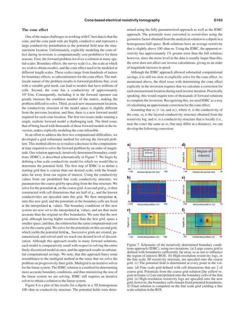
In an effort to address the first two computational difficulties, weeveloped a grid refinement method for solving the forward prob-em. This method allows us to realize a decrease in the computation-l time required to solve the forward problem by an order of magni-ude. Our solution approach, iteratively determined boundary condi-ions �IDBC�, is described schematically in Figure 7. We begin byefining a fine scale conductivity model for which we would like toetermine the potential field. The first step of IDBC is to define atarting grid that is coarser than our desired scale, with the bound-ries far away from our region of interest. Using the conductivityalues from our predefined fine scale conductivity structure, wearamaterize the coarse grid by upscaling from the fine structure. Weolve for the potentials uc on the coarse grid.Asecond grid gm is thenonstructed with cell dimensions that are half of gc, and the knownonductivities are upscaled onto this grid. We then interpolate uc

nto this new grid, and the potentials in the boundary cells are fixedt the interpolated uc values. The boundary conditions of this newystem are now set to the interpolated uc values, and are thus moreccurate than the original no-flux boundaries. We note that the newrid, although having higher resolution than the first grid, spans amaller space, and thus, the solution has the same computational costs for the coarse grid. We solve for the potentials on this second grid,hich yields the potential field um. Successive grids are created, pa-

ameterized, and solved until we reach our desired level of discreti-ation. Although this approach results in many forward solutions,ach model is comparatively small with respect to solving the entirenely discretized model at once, and the approach results in substan-

ial computational savings. We note, that this approach bares someesemblance to the multigrid method in the sense that we solve theroblem on progressively finer grids. Multigrid is an iterative solveror the linear system. The IDBC solution is a method for determiningore accurate boundary conditions, and thus minimizing the size of

he linear system we are solving. IDBC still requires an iterativeolver to obtain a solution to the linear system.

Figure 8 is a plot of the results for a dipole in a 3D homogenous00 ohm-m conductivity structure. The potential fields were deter-

ined using the fully parameterized approach as well as the IDBCpproach. The potentials were converted to resistivities using theeometric factor obtained from the analytical solution to a dipole in aomogenous half-space. Both solutions have an average resistivityhat is slightly above 100 ohm-m. Using the IDBC, the apparent re-istivity has approximately 1% greater error than the full solution;owever, since the noise level in the data is usually larger than this,he error does not affect our inverse calculations, giving us an orderf magnitude increase in speed.

Although the IDBC approach allowed substantial computationalavings, it is still too slow to explicitly solve for the cone effect. Asentioned above, the third issue with determining the cone effect

xplicitly in the inversion requires that we calculate a correction forach measurement location during each inverse iteration. Practicallypeaking, this would require tens of thousands of forward solutionso complete the inversion. Recognizing this, we used IDBC as a wayf calculating an approximate correction for the cone effect.

Assuming that �C� ��0 and �1�, where �c is the conductivity ofhe cone, �0 is the layered conductivity structure obtained from theesistivity log, and �1 is a conductivity structure that is locally �i.e.,ear the cone� the same as �0 �but may differ at a distance�, we canevelop the following correction:

igure 7. Schematic of the iteratively determined boundary condi-ions approach �IDBC�, using two iterations. �a� Large coarse grid isefined with boundaries sufficiently far away so as not to influencehe region of interest �ROI�. �b� High-resolution resistivity logs, orhe fine scale 3D resistivity structure, are upscaled onto the coarserid. �c� The potential field is determined at every point in the vol-me. �d� Fine scale grid defined with cell dimensions that are 1

2 ofoarse grid. Potentials from the coarse grid solution �the yellow re-ion in frame �c�� are interpolated onto the boundary cells of the finerid. �e� High-resolution resistivity logs are upscaled onto the newrid; however, the boundary cells remain fixed potential boundaries.f� Final solution is computed on the fine scale grid yielding a finecale solution in the ROI.

we

Ict

w

tcawcttcstsc

ctfmllst

lldeaatoev

tscccmtUtettwttrcc�imew

K

23mepises

Dft

Fi1tsm�c


ui��1 + �C� − ui��1� = ui��0 + �C� − ui��0� , �10�

here ui is the potential for at a given model point. Following fromquation 10, we obtain

ui��1 + �c� = 1 +ui��0 + �c� − ui��0�

ui��1�. �11�

f we assume that near the cone �1 � �0, which is reasonable be-ause �0 was derived from the resistivity logs, we can approximatehe cone effect with the following equation:

�12�

here Ci is the cone correction factor.From equation 12 we see that by comparing the potential field ob-

ained from a forward model ui��0 + �C� that explicitly includes theonductivity structure of the cone, with the potentials obtained frommodel that does not include the cone conductivity structure ui��0�,e can determine the modeling error associated with neglecting the

one in our model. For a new conductivity structure �1, that is a per-urbation about �0, we can use equation 12 to approximate the poten-ial field including the cone effect ui��1 + �C� without explicitly cal-ulating the cone effect for the new conductivity structure �1. As de-cribed above, the inversion algorithm is based on a linearization ofhe nonlinear problem, and therefore, we implicitly assume that ourtarting conductivity structure, for example �0, is close to the trueonductivity. In the case of C-bert, this a reasonable assumption be-

igure 8. Comparison of IDBC solution versus the fully parameter-zed solution; the solutions are for a dipole in a homogenous00 ohm-m media. The geometric factor has been applied to the po-ential fields, and thus, the entire image should be 100 ohm-m. �a� 2dlice thought the center of the 3D solution using the full solutionethod. �b� The same slice as in �a� solved using the IDBC approach.

c� The vertically averaged resistivities from �a� and �b�. �d� A per-ent difference map between �a� and �b�.

ause our starting model �0 is derived from the resistivity logs. Withhis in mind, we recognize that calculating the correction factor be-ore the inversion is a reasonable approach, because the startingodel for our inversion is close to the final model. Thus, if we calcu-

ate a correction factor for the starting model, it will be approximate-y correct for our final model. Moreover, forward modeling demon-trated that the magnitude of the cone effect was largely a function ofhe conductivity structure immediately adjacent to the cone.

To practically implement this correction, we created a high-reso-ution layered model, based on the RCPT log, for each C-bert surveyocation. This model can be considered locally correct because it iserived from the RCPT logs. Using IDBC, we calculated the coneffect at all measurement locations for each cone profile, solving onfinal grid that has cells around the cone location that are 10 mm onside. We then calculated the correction factor Ci, as shown in equa-

ion 12. The correction factor was incorporated into the interpolationperator Q, described in equation 4, thereby approximating the coneffect when the potentials are mapped to the data locations in the in-ersion.

Figure 9a is an example of a resistivity structure that we would ob-ain from an RCPT log. If we assume that the log represents a layeredystem, as depicted in Figure 9a, we can use the IDBC approach toalculate the C-bert data that we would obtain, while pushing theone into the subsurface, with and without explicitly including theone and cone rods. Figure 9b shows the results from such an experi-ent for a single current pair.As can be seen in Figure 9b, neglecting

he presence of the cone significantly changes our calculated data.sing the data presented in Figure 9b, we can generate a cone correc-

ion factor, as described above, and apply this correction to a differ-nt data set. Figure 9c shows a resistivity structure that is identical tohe one presented in Figure 9a, except for the presence of a conduc-ivity body a small distance from the cone location. As in Figure 9b,e present modeled data that consider the cone, and modeled data

hat ignore the cone; in addition, we include the results of applyinghe cone correction to the data that do not include the cone. The cor-ected data set is a good approximation to the data that explicitly in-lude the cone. Although this approximation works well for thisase, we stress that in the absence of a good local resistivity estimatee.g., the resistivity logs� this approach will not work. The corrections a linearization about the calibration model �e.g., the resistivity

odel in Figure 9a�. If the true model is far from the calibration mod-l, the linearization is not a good approximation and the correctionill fail.

idd 2 inversion results

For the Kidd 2 data set, we parameterized the inversions on a40 000 cell grid. The region of interest, a volume approximately0 � 35 � 30 m, contained approximately 74 000 cells with di-ensions of 0.75 m on a side. The remainder of the cells served to

nsure that we encountered minimal boundary effects. We ran multi-le inversions of the C-bert data that used slightly different regular-zation operators, as well as different initial guesses, and differenttarting values for the regularization parameter. The inversions tend-d to produce very similar results, and so we only show one of the re-ults here.

The starting model we used was based on the four resistivity logs.ue to a problem with the RCPT logging system, the resistivity log

rom C-bert 01 was discarded. The model was generated by first ver-ically upscaling each of the logs to 0.75-m grid cells, using geomet-

riit

tstafle

1btwdasawtstissetleobt

C

cttmt

tlfpsdhtsaul

hs

s5tcbep


ic averaging. The four upscaled logs were arithmetically averagedn the horizontal direction to create a layered starting model. Follow-ng this, the model values at the four resistivity log locations were seto the values from the corresponding upscaled logs.

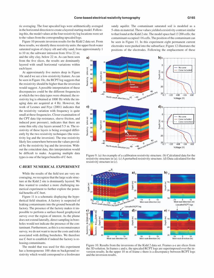
Figure 10 presents inversion results for the Kidd 2 data set. Fromhese results, we identify three resistivity units: the upper fresh wateraturated region of clayey silt and silty sand, from approximately 1o 10 m; the saltwater intrusion from 10 to 22 m;nd the silty clay, below 22 m. As can been seenrom the five slices, the results are dominantlyayered with small horizontal variations withinach layer.

At approximately five meters deep in Figure0c and d we see a low-resistivity feature. As cane seen in Figure 10c, the RCPT log suggests thathe resistivity should be higher than the inversionould suggest. A possible interpretation of theseiscrepancies could be the different frequenciest which the two data types were obtained; the re-istivity log is obtained at 1000 Hz while the im-ging data are acquired at 4 Hz. However, theork of Lesmes and Frye �2001� indicates that

he resistivity variation with frequency is quitemall at these frequencies. Closer examination ofhe CPT data �tip resistance, sleeve friction, andnduced pore pressure�, indicates that there areome thin silty clay layers around 5.5 m. The re-istivity of these layers is being averaged differ-ntly by the two resistivity techniques �the resis-ivity log and the inversion�. The true resistivityikely lies somewhere between the values provid-d by the resistivity log and the inversion. With-ut the coincident data, this interpretation woulde difficult to make. Acquiring multiple dataypes is one of the largest benefits of C-bert.

-BERT NUMERICAL EXPERIMENT

While the results of the field test are very en-ouraging, we recognize that the large scale struc-ure at the Kidd 2 site is dominantly layered. Wehus wanted to conduct a more challenging nu-

erical experiment to further explore the poten-ial benefits of C-bert.

Figure 11 is a schematic displaying the hypo-hetical field situation. A factory is suspected ofeaking contaminants into the ground beneath theactory. The presence of the factory makes it im-ossible to perform a surface-based geophysicalurvey over the region of interest. As the plumeoes not extend laterally, direct sampling in bore-oles would not indicate the presence of the con-aminant. Furthermore, as this is a reconnaissanceurvey, we do not want to incur the costs and risksssociated with drilling boreholes. We thereforese C-bert to establish if indeed the factory is re-easing contaminants.

The model that was used for this experimentas a homogeneous 100 ohm-m background re-istivity which would correspond to a freshwater

Figure 9. �a� Aresistivity struresistivity stru

Figure 10. Rethe 3D solutioversion resultand the invers

andy aquifer. The contaminant saturated soil is modeled as a-ohm-m material. These values yielded a resistivity contrast similaro that found at the Kidd 2 site. The model space had 13 200 cells; theontaminant occupied 116 cells. The position of the contaminant cane seen in Figure 11. In this experiment eight permanent currentlectrodes were pushed into the subsurface; Figure 12 illustrates theositions of the electrodes. Following the emplacement of these

ple of a calibration resistivity structure. �b� Calculated data for then �a�. �c�A perturbed resistivity structure. �d� Data calculated for then �c�.

om the inversions of the Kidd 2 data set. Frames a-e are slices fromames c and e, the upscaled RCPT logs are superimposed over the in-e upper 10 m of frame c there is a discrepancy between RCPT logsults.

n examcture icture i

sults frn. In frs. In thion res

ep1iiuGmewnr

tlmsdltmteCsctt

ibmc

Fleak directly beneath the factory.

Ftptdepth of 20 m.

Fsa


lectrodes, we obtained a series of eight C-bert data sets around theerimeter of the building. The C-bert locations can be seen in Figure2.Atotal of 4704 synthetic data points, 168 points for each of the 28ndependent current pairs, were calculated using the forward model-ng algorithm described above; these data were corrupted with 3%,niformly distributed, random noise. Data were inverted using theauss-Newton algorithm, described earlier.As with the field experi-ent, we used the RCPT logs to construct our starting model. How-

ver, as the cone never directly encounters the contaminant, the logsould suggest that the starting model for the inversion be a homoge-eous 100 ohm-m model. We used an isotropic flatness filter in theegularization.

Figure 13 illustrates the results of the inversion. As can be seen inhe figure, we clearly identified the presence of the contaminant be-ow the factory. This reconnaissance type of experiment highlights a

ajor potential benefit of C-bert, that is real-time experimental de-ign. All the RCPT data can be plotted in real time, so based on theseata, one can adapt the field sampling plan as more data come toight. Furthermore, as computational speed increases, we will even-ually be able to invert the C-bert data in the field, giving us 3D infor-

ation that can be used to guide and adapt our survey design. Forhis example, if it were found that the contaminant was migrating lat-rally, we could quickly adapt our sampling strategy, and acquire-bert data sets that would allow us to image the migration. The re-

ults of a survey such as this may help to rapidly design a plan forlean-up at the site. In addition, these results could be used to guidehe emplacement of a more expensive, permanent ERT array for longerm monitoring.

SUMMARY AND CONCLUSIONS

The focus of this work was an assessment of a cone-based imag-ng system for obtaining 3D images of electrical conductivity. Cone-ased imaging is advantageous for several reasons. First, it is a mini-ally invasive way to obtain information about the subsurface 3D

onductivity structure. Second, using a small number of sourceterms �e.g., for the Kidd 2 study there were a totalof only 36 current pairs�, while measuring multi-ple data points, can potentially result in faster in-versions. Third, we obtain multiple colocateddata, which better constrains inverse results andassists in interpretation. Finally, field acquisitionof C-bert data lends itself well to real time experi-mental design allowing one to chose new test lo-cations as more information comes to light.

The Kidd 2 field study has successfully demon-strated that C-bert data can be used to image thenear subsurface. We have outlined the requiredfield equipment and testing procedures necessaryfor acquiring these data. The equipment used forthis survey required minor modifications of exist-ing RCPT systems. Interpretation of the data,however, required the development of a cone-ef-fect correction, which in turn required a computa-tionally efficient solution to the forward problem.The iteratively determined boundary conditionsapproach, IDBC, was developed to facilitate thiscorrection, by allowing us to solve the forwardproblem considerably faster than with a fully pa-rameterized approach. The use of IDBC extends

are west-eastmes b and b�respectively.

igure 11. Schematic of the synthetic problem. There is a suspected

igure 12. Eight permanent electrodes are placed around the perime-er of the factor. Four are situated at depths of 4 m and four arelaced at 8 m. Eight C-bert profiles are acquired around the perime-er, as indicated by the figure. C-bert profiles were acquired to a

igure 13. Inversion results for the synthetic experiment. Frames a and a�lices through the synthetic model and the inverse result, respectively. Frare depth slices, at 6 m, through the synthetic model and the inverse results,

bt

cToufiksmdwat

2sbClfs

St0mpsUrcttp

B

C

C

D

D

H

H

H

H

J

—

J

K

L

L

L

N

N

N

S

S

S

S

V

Z


eyond simply solving for the cone effect; it can be used as an effec-ive solver for the general Poisson’s equation.

While in this pilot study we collected only five C-bert data sets, weould easily obtain tens of C-bert data sets in a full-scale field survey.he RCPT logs associated with each of these C-bert data sets are notnly valuable for building an accurate starting model, but also gives the potential to generate more informed regularization operatorsor our inversions. In over-parameterized inverse problems we mustnject some a priori knowledge in order to solve them. A priorinowledge, based on in-situ, site specific measurements, is more de-irable than derivative type filters, but in general, these measure-ents are difficult to obtain. The colocated data that are acquired

uring the C-bert process serve this purpose. As shown with ourork, they can be used as constraints within our regularization oper-

tors, and to construct an informed reference model that is used inhe regularization.

We were very encouraged by the results of the field test at the Kiddsite. We recognized, however, that the relatively simple layered

tructure at the site did not allow us to fully demonstrate the potentialenefits of C-bert. Our synthetic example illustrates the ability of-bert to determine conductivity values in regions that are not readi-

y accessible to other forms of measurement. We believe that, withurther refinement, C-bert will become a useful tool for acquiringubsurface conductivity images.

ACKNOWLEDGMENTS

Partial funding for this project came from a McGee grant, from thechool of Earth Sciences at Stanford University and a DOE Grant

hrough Emory University �DOE CAREER Grant DE FG025ER25696�. We thank John Howie for the use of the UBC Depart-ent of Civil Engineering cone truck, and for his input on the inter-

retation of the RCPT data. The field work would not have been pos-ible without the assistance of Ali Amini and Scott Jackson from theBC Department of Civil Engineering. We extend thanks to three

eviewers for providing such excellent reviews of this paper; theirontributions greatly enhanced this manuscript. In particular wehank Partha Routh, who completed a detailed review and providedhe derivation for the cone correction that has been included in thisaper.

REFERENCES

inley, A., G. Cassiani, R. Middleton, and P. Winship, 2002, Vadose zoneflow model parameterisation using cross-borehole radar and resistivityimaging: Journal of Hydrology, 267, 147–159.

ampanella, R. G., and I. Weemees, 1990, Development and use of an elec-trical resistivity cone for groundwater contamination studies: CanadianGeotechnical Journal, 27, 557–567.

lague, J. J., J. L. Luternauer, and R. J. Hebda, 1983, Sedimentary environ-ments and postglacial history of the Fraser Delta and lower Fraser Valley,
British Columbia: Canadian Journal of Earth Sciences, 20, 1314–1326.
aily, W., and A. Ramirez, 1995, Electrical-resistance tomography duringin-situ trichloroethylene remediation at the Savanna river site: Journal ofApplied Geophysics, 33, 239–249.

aniel, C. R., H. L. Giacheti, J. A. Howie, and R. G. Campanella, 1999, Re-sistivity piezocone �RCPTU� data interpretation and potential applica-tions: Proceedings of the XI Panamerican Conference on Soil Mechanicsand Geotechnical Engineering, 361–368.

aber, E., U. M. Ascher, D. A. Aruliah, and D. W. Oldenburg, 2000a, Fastsimulation of 3D electromagnetic problems using potentials: Journal ofComputational Physics, 163, 150–171.

aber, E., U. M. Ascher, and D. Oldenburg, 2000b, On optimization tech-niques for solving nonlinear inverse problems: Inverse Problems, 16,1263–1280.

ofmann, B. A., 1997, In situ ground freezing to obtain undisturbed samplesof loose sand for liquefaction assessment: Ph.D. thesis, University of Al-berta.

unter, J. A., S. E. Pullman, R. A. Burns, R. L. Good, J. B. Harris, A. Pugin,A. Skvortsov, and N. N. Goriainov, 1998, Downhole seismic logging forhigh-resolution reflection surveying in unconsolidated overburden: Geo-physics, 63, 1371–1384.

arvis, K. D., and R. Knight, 2000, Near-surface VSP surveys using the seis-mic cone penetrometer: Geophysics, 65, 1048–1056.—–, 2002, Aquifer heterogeneity from SH-wave seismic impedance inver-sion: Geophysics, 67, 1548–1557.

arvis, K., R. J. Knight, and J. A. Howie, 1999, Geotechnical applications ofVSP surveys using the seismic cone penetrometer: Proceedings of theSymposium on the Application of Geophysics to Engineering and Envi-ronmental Problems, 11–20.

emna, A., J. Vanderborght, B. Kulessa, and H. Vereecken, 2002, Imagingand characterisation of subsurface solute transport using electrical resis-tivity tomography �ERT� and equivalent transport models: Journal of Hy-drology, 267, 125–146.

aBrecque, D. J., and X. Yang, 2001, Difference inversion of ERT data; Afast inversion method for 3-D in situ monitoring: Journal of Environmen-tal & Engineering Geophysics, 6, 83–89.

esmes, D. P., and K. M. Frye, 2001, Influence of pore fluid chemistry on thecomplex conductivity and induced polarization responses of Berea sand-stone: Journal of Geophysical Research, 106, 4079–4090.

unne, T., P. K. Robertson, and J. J. M. Powell, 1997, Cone penetration test-ing in geotechnical practice: BlackieAcademic & Professional.

arbutovskih, S. M., W. D. Daily, R. M. Morey, and R. S. Bell, 1997, Test re-sults of CPT-deployed vertical electrode arrays at the DOE Hanford Site:Proceedings of the Symposium on the Application of Geophysics to Engi-neering and Environmental Problems, 21–31.

eilson-Welch, L., 1999, Saline water intrusion from Fraser River estuary:Ahydrogeological investigation using field chemical data and a density-de-pendent groundwater flow model: M.S. thesis, University of British Co-lumbia.

eilson-Welch, L. and L., Smith, 2001, Saline water intrusion adjacent to theFraser River, Richmond, British Columbia: Canadian Geotechnical Jour-nal, 38, 67–82.

aad, Y., 1996, Iterative methods for sparse linear systems: PWS PublishingCompany.

ingha, K., and S. M. Gorelick, 2005, Saline tracer visualized with electricalresistivity tomography: Field scale spatial moment analysis: Water Re-sources Research, 41, W05023.

later, L., A. M. Binley, W. Daily, and R. Johnson, 2000, Cross-hole electri-cal imaging of a controlled saline tracer injection: Journal ofApplied Geo-physics, 44, 85–102.

later, L., A. Binley, R. Versteeg, R. G. Cassiani, R. Birken, and S. Sandberg,2002, A 3D ERT study of solute transport in a large experimental tank:Journal ofApplied Geophysics, 49, 211–229.

ersteeg, R., R. Birken, S. K. Sandberg, and L. Slater, 2000, Controlled im-aging of fluid flow and a saline tracer using time lapse GPR and electricalresistivity tomography: Proceedings of the Symposium on theApplicationof Geophysics to Engineering and Environmental Problems, 283–292.

hang, J., R. L. Mackie, and T. R. Madden, 1995, 3-D resistivity forwardmodeling and inversion using conjugate gradients: Geophysics, 60,
1313–1325.

cone-based electrical resistivity tomographyhaber/pubs/pidlisecky_knight_haber_2006.pdf ·...

Documents