CONE BEAM COMPUTED TOMOGRAPHY THREE-DIMENSIONAL

RECONSTRUCTION FOR EVALUATION OF THE

MANDIBULAR CONDYLE

Brian Albert Schlueter, D.M.D.

An Abstract Presented to the Faculty of the Graduate School

of Saint Louis University in Partial Fulfillment of the Requirements for the Degree of

Master of Science in Dentistry

2007

1

Abstract

Cone beam computed tomography (CBCT) has proven to

be a valuable imaging modality for examination of the

temporomandibular joint (TMJ). CBCT three-dimensional (3D)

reconstructions potentially provide the clinician with

efficient and effective means for evaluation of the

mandibular condyle. The purpose of the present study is to

investigate what the ideal Hounsfield unit values are for

the examination of the condyle; and if an ideal window

width and level can be identified, can one reliably

evaluate the mandibular condyle using the CBCT 3D

reconstruction?

Linear dimensions between six anatomical sights

were measured with a digital caliper to assess the anatomic

truth for 50 dry human mandibular condyles. Condyles were

scanned with the i-CAT (Imaging Sciences International,

Hatfield, PA) CBCT; and image reconstruction and assessment

was accomplished using V-works™4.0 (Cybermed Inc, Seoul,

Korea). Three linear three-dimensional measurements were

made on each of the 50 condyles at eight different

Hounsfield unit (HU) windows. These measurements were

compared with the anatomic truth. Volumetric measurements

were also completed on all 50 condyles, at 23 different

2

window levels, in order to define the volumetric

distribution of bone mineral density (BMD) within the

condyle. Significance testing for 3D linear measurement

and volumetric differences was accomplished using

independent t-tests with a 95% confidence interval.

Significant differences were found in two of the

three linear measurement groups at and below the

recommended viewing window for osseous structures. The

most accurate measurements were made within the soft tissue

range for HU window levels. Volumetric distribution

measurements revealed that the condyles were mostly

comprised of low density bone; and that condyles exhibiting

significant changes in linear measurements were shown to

have higher percentages of low density bone than those

condyles with little change from the anatomic truth.

Assessment of the mandibular condyle, using the 3D

reconstruction, is most accurate when accomplished at

density levels below that recommended for osseous

examination. Utilizing lower window levels, extending into

the soft tissue range, may compromise one’s capacity to

view the bony topography. This would suggest that CBCT 3D

reconstructed images, by themselves, may not be a reliable

means for the diagnosis condylar pathology, and or changes

in condylar morphology.

3

CONE BEAM COMPUTED TOMOGRAPHY THREE-DIMENSIONAL

RECONSTRUCTION FOR EVALUATION OF THE

MANDIBULAR CONDYLE

Brian Albert Schlueter, D.M.D.

A Thesis Presented to the Faculty of the Graduate School

of Saint Louis University in Partial Fulfillment of the Requirements for the Degree of

Master of Science in Dentistry

2007

i

COMMITTEE IN CHARGE OF CANDIDACY: Assistant Professor Ki Beom Kim, Chairperson and Advisor Assistant Professor Donald R. Oliver, Professor Gus G. Sotiropoulos

ii

DEDICATION

I dedicate this thesis project to my wife Hollie and our sons Noah and Parker.

iii

ACKNOWLEDGEMENTS

In acknowledgement of the people who have helped on

this thesis project. I would like to thank Dr. Ki Beom Kim

for his constant support and dedication through the entire

process. I would also like to thank Drs. Donald Oliver and

Gus Sotiropoulos for devoting their time, knowledge, and

encouragement along the way. Also, this project would not

have been possible without the help of Dr. Cyrus Alizadeh,

Dr. Becky Schreiner and the Alizadeh Orthodontics staff.

Thank you for your gracious hospitality and selfless

contribution to help make this project a success. Finally,

thanks to Drs. Heidi Israel and Binh Tran for their help

with the statistical analysis of the data.

iv

TABLE OF CONTENTS

List of Tables............................................vi List of Figures..........................................vii CHAPTER 1: INTRODUCTION....................................1 CHAPTER 2: REVIEW OF THE LITERATURE Development of Dental Radiographic Imaging......5 X-Ray .........................................5 Cephalometry ..................................6 Panoramic Radiography .........................7 Tomography ....................................9 Computed Tomography ..........................12 Cone Beam Computed Tomography ................17 Conventional CT vs. CBCT.......................19 Imaging Performance ..........................21 Radiation Dosimetry ..........................25 Size and Cost ................................28 CBCT Orthodontic Applications..................30 Accuracy .....................................30 Impacted Teeth and Oral Abnormalities ........34 Airway Analysis ..............................38 Orthognathic Surgery .........................40 Temporomandibular Joint Evaluation: Imaging...41 2D Imaging ...................................43 3D Imaging ...................................47

Hounsfield Units as a Measure of Bone Density Distribution .................................50

References.....................................62 CHAPTER 3: JOURNAL ARTICLE................................70 Abstract.......................................70 Introduction...................................72 Materials and Methods..........................76 Selecting the Sample .........................76 Imaging ......................................77 Isolating and Measuring the Condyle ..........79 Volume Measurements at Varying Window Widths .86 Data analysis ................................89 Results........................................91 Discussion.....................................95 Conclusions...................................102 Acknowledgements..............................104 Literature Cited..............................105

v

Vita Auctoris............................................109

vi

List of Tables

Table 2.1: Window widths for density values and Hounsfield numbers in the body............61

Table 3.1: Hounsfield Unit window widths (w) used to

create 3D renderings of the condyles. 3D linear measurements were accomplished on each of these renderings................................80

Table 3.2: Definitions of condylar linear

measurements..............................82 Table 3.3: Definitions of anatomic landmarks.........82 Table 3.4: Hounsfield Unit window widths (WW) used to

create 3D condyle renderings for volumetric evaluation. Window 24 is equal to the sum of window widths 1-23.....................89

Table 3.5: Hounsfield Unit window widths (WW) used to

create 3D condyle renderings for volumetric measurements (see Table 3.4). CL1 represents the average % volume of the condyles that showed the greatest change in condylar length measurement at 176 HU–2476 HU. CL0 was the least change in condylar length measurement. CW1 was the greatest change in condylar width, and CW0 the least.....................................91

Table 3.6: Hounsfield Unit window widths (W) used to

create 3D condyle renderings for linear measurements (see Table 3.1 for W ranges). Average condylar length (CL), condylar Width (CW), and condylar height (CH) are compared with the gold standard (GS)...............93

Table 3.7: Comparison (Independent t-tests) of

volumetric measurements: CL0 vs. CL1, and CW0 vs. CW1 at twenty-three window levels....................................94

Table 3.8: Window widths for density values and

Hounsfield numbers in the body............99

vii

List of Figures Figure 1.1: A multiplanar reconstruction (MPR) with

axial, coronal, and sagittal crossectional views, as well as 3D reconstruction view...3

Figure 2.1: Early laboratory CT machine, with x-ray

tube, designed by Godfrey N. Hounsfield (image adopted and modified from Godfrey N. Hounsfield’s Nobel lecture, 8 December, 1979).....................................14

Figure 2.2: First clinical CT scanner prototype

installed at Atkinson Morley Hospital in London, 1971 (image adopted and modified from Godfrey N. Hounsfield’s Nobel lecture, 8 December, 1979).........................14

Figure 2.3: Graphic representation of the image acquisition technique the conventional CT fan shaped beam and the CBCT cone shaped beam......................................19

Figure 2.4: Images adopted and modified from 3D

Diagnostix Inc. and IMTEC Imaging.........20 Figure 2.5: Scale used by Hounsfield to demonstrate the

accuracy to which absorption values can be ascertained on the CT picture.............52

Figure 2.6: Hounsfield Scale of CT Numbers (image taken

from Jackson).............................53 Figure 2.7: 3D reconstruction (197 HU to 2476 HU).....58 Figure 2.8: 3D reconstruction (-100 HU to 2476 HU)....58 Figure 2.9: 3D reconstruction (-200 HU to 2476 HU)....58 Figure 2.10: 3D reconstruction (-400 HU to 2476 HU)....59 Figure 2.11: 3D reconstruction (-600 HU to 2476 HU)....59

viii

Figure 2.12: These photographs of the mandible shown in the previous reconstruction images demonstrate the true appearance of the articular surfaces of the right condyle. a) lateral pole, b) posterior surface, c) right mandible, d) posterior/lingual view right half of the mandible......................60

Figure 3.1: A multiplanar reconstruction (MPR) with

axial, coronal, and sagittal crossectional views, and 3D reconstruction..............74

Figure 3.2: Anatomical landmarks: a) anterior view of

condyle showing medial mandibular condyle (MCo) and lateral mandibular condyle (LCo), b) lateral view of condyle showing posterior mandibular condyle (PCo), anterior mandibular condyle (ACo), and superior mandibular condyle (SCo), c) lingual view of the ramus showing lingula (L).............77

Figure 3.3: 3D Reconstruction isolation: a) Initial

lateral view 3D reconstruction, b) Frankfort Horizontal initial sculpting cut, c) Vertical sculpting cuts, d) Completed isolation for condylar measurements.......81

Figure 3.4: Point-to-point linear measurements on the 3D

reconstruction in V-works™4.0 SSD mode; a) Condylar width (CW), b) Condylar length (CL), and c) Condylar height..............83

Figure 3.5: Lateral view of plane construction........84 Figure 3.6: Superior view of plane construction.......85 Figure 3.7: Anterior view of plane construction with

(CW) measurement..........................85 Figure 3.8: 3D reconstruction isolation for volumetric

measurements of the mandibular condyle: a) initial cut parallel to Frankfort Horizontal, b) second cut parallel to the first cut at the level of the most inferior point in the sigmoid notch, c & d) lateral and oblique views of the final isolated reconstruction............................87

ix

Figure 3.9: Anterior and lateral volumetric renderings of the right condyle at four different window widths: a) 176-2476 HU, b) 376-475 HU, c) 1476-1575 HU, d) 1976-2075 HU......88

Figure 3.10: Distribution of % Differences between 3D

linear measurements and gold standards (GS); a) CW measurement % differences in W8 (176-2476 HU) with mean group (yellow) between the red lines, b) CL measurement differences in W8 with mean group (yellow) between the red lines.................................92

Figure 3.11: Distributions of condylar volume in twenty-

three window widths for the condyles of groups CL1 and CL0, Window 1 represents the lowest density bone, and window 23 being the highest density bone observed.............96

Figure 3.12: Distributions of condylar volume in twenty-

three window widths for the condyles of groups CW1 and CW0, Window 1 represents the lowest density bone, and window 23 being the highest density bone observed.............97

1

CHAPTER 1: INTRODUCTION

Temporomandibular joint (TMJ) standard radiographic

studies such as the plain film radiography and panoramic

radiography have little capacity to reveal anything more

than gross osseous changes1 within the joint; and therefore,

in some cases a more comprehensive radiographic study is

indicated. Radiographic analysis of the TMJ is a broad

field and is considered by some to be a separate subset of

oral and maxillofacial radiology,2 consisting of both two

and three-dimensional imaging modalities. Two-dimensional

(2D) imaging of the TMJ employs conventional radiology to

produce a variety of projections. The submental-vertex,

lateral transcranial, transpharyneal, transmaxillary (AP),

as well as conventional tomography are a few examples of

the 2D studies used in TMJ evaluation. Three-dimensional

evaluations, such as computed tomography (CT) and magnetic

resonance imaging (MRI), have been utilized to some degree;

however, historically, high cost,3,4 large radiation

dosage,5,6 large space requirements,3,4 and the high level of

skill required for interpretation have kept its use to a

minimum. With the introduction of limited cone-beam

technology, such deterrents of CT imaging have been greatly

2

diminished. With five different cone-beam computed

tomography (CBCT) scanners now available on the world

market, lower radiation dosages,7-10 and lower costs,3 3D

radiography is likely to become more commonplace in the

dental profession. Demonstrating a broad spectrum of

applications and vastly improved accuracy over 2D

radiography,4,11,12 CBCT proves to be an invaluable diagnostic

tool for the evaluation of the osseous structures of the

TMJ.

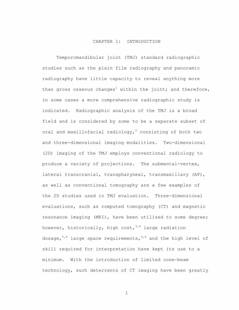
Three-dimensional imaging facilitates comprehensive

examination of the subarticular osseous surfaces of the TMJ

through two different viewing modalities. One allows for

the tissue of interest to be examined through progressive

crossectional slices in a chosen plane of orientation;

while the other produces 3D reconstructions capable of

being manipulated in any given direction, thereby

facilitating and expediting the examination procedure.

Often, these two viewing methods are combined into what is

referred to as the multiplanar reconstruction (MPR). MPR

viewing mode enables the examiner to simultaneously assess

crossectional and three-dimensionally reconstructed images

(see Figure 1.1).

Within the condyle there is variation in bone

density and composition. Cortical bone, trabeculae, and

3

Figure 1.1. A multiplanar reconstruction (MPR) with axial, coronal, and sagittal crossectional views, as well as 3D reconstruction view.

intertrabecular tissues have varying densities and

mechanical properties.13-17 These differences present a

challenge when examining the bony subarticular surfaces of

the condyle with 3D CT imaging. For computed tomography

density is often expressed in the form of CT Numbers or

Hounsfield Units. From radiation intensity readings

acquired in the scanning process, the density or

attenuation values of tissues of interest can be

calculated. The attenuation coefficients are normalized

with respect to water as the reference material, and a

magnifying constant is then applied to produce a CT

number.18 Hounsfield19 originally described the Hounsfield

4

Unit (HU) as an absorption value; and he constructed a

scale to demonstrate the accuracy to which the absorption

values could be ascertained on a visual image. For the

machine he described,19 the scale ranged from air (-1000) at

the bottom of the scale, to bone (1000) at the top of the

scale. Each number represents a different shade of gray

within the spectrum. The range of tones between black and

white seen in an image can be limited to a large or small

window within the scale. This window can then be raised or

lowered depending upon the absorption value of the material

of interest19. The examiner must be able to decide what

window level and width will most accurately represent the

anatomical truth of a tissue under examination. It is

important for the clinician to be able to reliably detect

osseous abnormalities such as cortical erosion,

osteophytosis, osteoarthritis, and sclerosis. The purpose

of the present study is to investigate what the ideal

Hounsfield unit values are for the examination of the

condyle; and if an ideal window width and level can be

identified, can one reliably evaluate the subarticular

anatomy of the mandibular condyle using the CBCT 3D

reconstruction?

5

CHAPTER 2: REVIEW OF THE LITERATURE

Development of Dental Radiographic Imaging

X-Ray

X-rays were an accidental discovery made by Wilhelm

Conrad Roentgen on November 8, 1885.20 The discovery was

made while he was studying cathode rays in a high-voltage,

gaseous-discharge tube (Crookes tube). He discovered that

a nearby barium-platinocyanide screen began to fluoresce

when the tube was in operation. From this he decided that

the fluorescence was the result of an invisible form of

radiation with greater penetrating capacity than

ultraviolet rays.21 To identify this invisible form of

radiation Roentgen, coined the term “X-ray”. “X”, being

the unknown variable in mathematic equations, was an

appropriate name for these rays with an unknown nature.22

The X-ray was first introduced to the world when Roentgen

published his first paper: “On a New Kind of Ray, A

Preliminary Communication” (1895). Soon after, in 1901, he

was awarded the Nobel Prize for his revolutionary work with

X-rays.20

The discovery of X-rays had a profound effect on a

myriad of industries including, but not limited to, the

6

medical and dental professions. The year following

Roentgen’s first publication, C. Edmund Kells became the

first American dentist to take dental radiographs of a

living subject. He was also the first to exhibit the

dental X-ray apparatus at a dental meeting; thereby

introducing this new diagnostic capability to the dental

profession.22,23

Cephalometry

Radiographic cephalometry was introduced by Pacini

in 1922 for anthropometric purposes.24 He made the process

somewhat reproducible by immobilizing the head and using

set source to object and object to film distances. This

provided a means for visualizing the anatomy; however, it

gave no measurability, and the reproducibility was

questionable. Just four years later an orthodontist named

B. Holly Broadbent adapted the roentgenographic craniometer

as a means to stabilize the heads of living subjects in a

fixed position for imaging. Previously, the craniometer or

craniostat, developed by Dr. T. Wingate Todd, was used

solely for holding skulls in a fixed position while precise

lateral and posteroanterior radiographs were made.25

Broadbent introduced his head holder for roentgenographic

studies of the living head26 in his 1931 paper: “A New X-Ray

7

Technique and Its Application to Orthodontia” The nuance

of Broadbent’s roentgenographic cephalometry revolutionized

orthodontics; making it possible for the clinician to

obtain standardized and accurate measurements from lateral

and posteroanterior radiographs. These two-dimensional (2D)

images have been used to study craniofacial growth, facial

types, and relationships of the jaws; teeth, and soft

tissues, and the positioning and morphology of various

other bony structures. They also aid in treatment

planning, forecasting future relationships, and evaluating

the results of growth and treatment. Cephalometry is the

only practical imaging technique that allows the

investigator to quantitatively evaluate of the spatial

relationships between cranial and dental structures.2 For

this reason cephalometry has remained relatively unchanged

today.

Panoramic Radiography

Prior to the development of the panoramic

radiograph there was no practical way to image the jaws and

teeth in one film. Panoramic radiography originated from

the need to accurately image the jaws in their entirety on

a single film. Attempts made to accomplish this began in

1922 when A. F. Zulauf (USA) described and patented a

8

method whereby a narrow beam scanned the upper or lower jaw

to create a panoramic image. He named this device “the

panoramic x-ray apparatus”. Shortly after, in 1933, H.

Numata (Japan) constructed a device suitable for clinical

examinations and labeled his method “parabolic

radiography”. These earlier forms of panoramic radiography

utilized intraoral film which resulted in various practical

problems.27 However, in 1949, Y. V. Paatero (Finland)

published papers describing the basic principles of

panoramic radiography using extraoral film. Paatero worked

closely with an engineer by the name of T. Niemien, to

further develop the technique; and their close

collaboration continued until Paatero’s death in 1963.

Production of the first commercial equipment began in 1960

with the introduction of the Orthopantomograph. Niemien

was the driving force behind its development and marketing;

and the manufacturer was established under the name Palomex

(Panoramic Layer Observing Machine for Export).

Development and technological advancement of the equipment

and technique continued, and in 1988 the Scanora device

(Orion Corporation/Soredex, Finland) was introduced. It

was the first machine to combine panoramic radiography and

multidirectional tomography; thereby, providing the

clinician with the ability to acquire cross-sectional

9

images of the jaws.27 Panoramic radiography, however, has

many shortcomings related to the reliability and accuracy

of size, location, and form of the images created. The

origin of these shortcomings lies in the design of the

technique. The panoramic image is made by creating a focal

trough or region of focus within a generic jaw form and

size. The most reliable images are obtained when the

subjects jaw form and size most closely approximate the

generic jaw form and size. Anything outside this will

introduce error in the image produced.2

Tomography

Film based tomography (analog tomography) was

designed for the purpose of creating clearer images of

objects lying within a particular plane of interest.28 The

technique to produce a tomogram is very similar to that of

the panograph in that the X-ray tube moves in the opposite

direction of the film cassette on the other side of the

patient. During the rotation only one section of tissue

remains in focus, while tissues above or below the section

are blurred by the motion of the tube and cassette.29

Though, the concept of tomography had been

described as early as 1914 by a Polish radiologist named

Mayer, the first true analog tomograms were not constructed

10

until the early 1930s. In Vallebona’s 1930 paper he

described a tomographic x-ray unit in which the tube and

cassette remained stationary and the patient rotated

between them. Three years later he constructed a unit in

which the patient remained stationary and the tube and

cassette rotated around. This device produced images of

little diagnostic capability in that only the structures

along the axis of rotation remained in focus. Around the

same time as Vallebona, the Dutch physician Ziedses des

Plantes, recognized today as the founder of modern analog

tomography, introduced linear, pluridirectional and

multisection tomography.

Pluridirectional tomographic motion yielded fewer

image artifacts than did the linear motion utilized in

earlier machines. The sectional images produced with this

technique were recognized with many names including:

planigraphy, stratigraphy, laminagraphy, body select

radiography, and zonography.29 Tomography evolved as a

method to overcome undesirable superimpositions that are

difficult to eliminate in plane film radiography. One

example of this is presented with the complex angulations

required in the transmaxillary technique to avoid

superimposition of the mastoid process on the joint image.30

11

The first American tomographic unit was developed

by Andrews of the Cleveland Clinic in 1936. Shortly after,

Keiffer and Moore constructed the tomographic laminagraph

at the Mallinckrodt Institute in St. Louis, MO. It wasn’t

until 1949 that a tomographic machine was made commercially

available; and was reproduced under the name “Polytome” by

Masslot. Soon after, hypocycloidal motion was added to

this unit, and through marketing by Phillips, it became the

gold standard of analog tomography.29 This and other

complex movements such as circular and ellipsoid, found on

newer computer controlled machines, helped to minimize the

problems presented in earlier machines that used linear or

straight line movement patterns. These more simplistic

movements tended to degrade the overall image sharpness.1,30

These images often appear streaked. Streaks appear when

the long axis of a structure lying outside the focal plane

is oriented parallel to the movement of the tube.28,30

Modern, complex-motion tomographic units can be optimized

to image any selected region of the facial skeleton.2 They

provide sharper images, greater density uniformity,

consistent magnification, and increased dimensional

stability.28 Though quite versatile in their applications,

images produced with analog tomography are limited to one

plane or slice of the anatomy under study. They have no

12

capability of combining slices to create an appearance of

three-dimensional (3D) form as in computed tomography.

Computed Tomography

Computed Tomography (CT) is essentially an advanced

form of tomography that utilizes computerized storage of

data from a series of thin tomographic sections taken from

multiple directions. The exposures are recorded by an

array of sensors positioned on the opposite side of a

rotating gantry from the radiation source.30 The principle

of CT evolved from the work of an Austrian mathematician,

Radon, who demonstrated in 1917 that a 3D image of an

object could be reconstructed from an infinite number of

two-dimensional (2D) projections. His work focused on

equations that described gravitational fields, and had

nothing to do with medical imaging.29

In the late 1960s and early 1970s several groups

were investigating tomographic imaging from projections as

a possible diagnostic tool, or potential aid in treatment

planning and radiation therapy. Godfrey Hounsfield, an

engineer at the Central Research Laboratories of Electro-

Musical Instruments (EMI) Ltd. in England, brought this

technology to a clinical reality in the early 1970s. His

first experimental apparatus yielded reasonable images of a

13

symmetrical object; however, the time required for a scan

was excessive, taking up to 9 days for data acquisition and

another 2.5 hours for data processing. Much of this was a

result of the low intensity of the radiation provided by

the Am-241 x-ray source used in this early apparatus. Soon

after, Hounsfield replaced the Am-241 source with an x-ray

tube and reduced the data acquisition time from 9 days to 9

hours29 (Figure 2.1). This was still too long to make

diagnostically adequate images of the abdomen due to the

constant motility that occurs in the gastrointestinal

track. Instead, the first CT scanner Hounsfield developed

for humans focused on the brain as the target organ (Figure

2.2). In October 1971 the first image was obtained at the

Atkinson Morley Hospital in London. The scan, with a data

acquisition of 4.5 minutes, clearly revealed a frontal lobe

tumor in a 41 years old woman.29

There are two CT scanner configurations: one where

both the x-ray tube and the detector array revolve around

the patient, and the other where only the x-ray tube

rotates; and radiation detection is accomplished by the use

of a fixed circular array of detectors.28,30,31 The later

configuration often utilizes greater than one thousand

detectors; and newer generations often incorporate multiple

rows of detector rings; making it possible to acquire

14

Figure 2.1. Early laboratory CT machine, with x-ray tube, designed by Godfrey N. Hounsfield (image adopted and modified from Godfrey N. Hounsfield’s Nobel lecture, 8 December, 1979)19

Figure 2.2. First clinical CT scanner prototype installed at Atkinson Morley Hospital in London, 197119 (image adopted and modified from Godfrey N. Hounsfield’s Nobel lecture, 8 December, 1979).19

15

multiple slices per tube rotation.31 This type of CT

scanner incorporates slip ring technology which enables the

x-ray tube to rotate continuously around the subject in one

direction. The path the tube makes around the subject is a

spiral or helical pattern; hence the name spiral or helical

CT. This allows larger anatomical regions of the body to

be imaged during a single breath hold, thereby reducing the

possibility of movement artifacts.31 Since the introduction

of Hounsfield’s first prototype, there has been a gradual

evolution to five generations of such systems. Each system

is classified on the organization of the individual parts

of the device and the physical motion of the beam in data

acquisition.7

CT offers several distinct advantages over

conventional film tomography. The first of these is its

ability to produce images completely devoid of

superimpositions from structures superficial or deep to the

area of interest. Second, due to the high contrast

capabilities of CT images, differentiation between tissues

with density differences of less than 1% can be

distinguished. Conversely, conventional film radiography

requires a 10% physical density difference for the examiner

to be able to distinguish between tissues. The third of

these advantages is demonstrated through its ability to

16

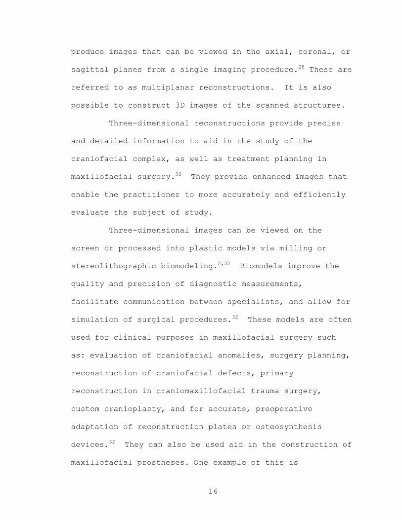
produce images that can be viewed in the axial, coronal, or

sagittal planes from a single imaging procedure.28 These are

referred to as multiplanar reconstructions. It is also

possible to construct 3D images of the scanned structures.

Three-dimensional reconstructions provide precise

and detailed information to aid in the study of the

craniofacial complex, as well as treatment planning in

maxillofacial surgery.32 They provide enhanced images that

enable the practitioner to more accurately and efficiently

evaluate the subject of study.

Three-dimensional images can be viewed on the

screen or processed into plastic models via milling or

stereolithographic biomodeling.2,32 Biomodels improve the

quality and precision of diagnostic measurements,

facilitate communication between specialists, and allow for

simulation of surgical procedures.32 These models are often

used for clinical purposes in maxillofacial surgery such

as: evaluation of craniofacial anomalies, surgery planning,

reconstruction of craniofacial defects, primary

reconstruction in craniomaxillofacial trauma surgery,

custom cranioplasty, and for accurate, preoperative

adaptation of reconstruction plates or osteosynthesis

devices.32 They can also be used aid in the construction of

maxillofacial prostheses. One example of this is

17

temporomandibular joint replacement prosthetics; which

often involves replacement of the condyle and in some cases

the glenoid fossa.

Cone Beam Computed Tomography

Computed tomography has proven to be quite helpful

for dental diagnosis, however, conventional helical-CT

units were not originally developed for this purpose. The

problems in adapting helical-CT scans for dental use

include: high cost, large space requirement, long scanning

time, high radiation exposure, and low resolution in the

longitudinal direction compared with it’s relatively high

resolution in the axial direction.33-35 The last of these is

a result of the method by which longitudinal images are

produced, through summation of axial CT images.35 Each

axial slice is produced by one revolution of the fan shaped

beam of x-rays. Then, the axial slices are stacked in

order to create a complete image of the object under study.

In 1997, the Department of Radiology in the Nihon

University School of Dentistry set out to resolve some of

shortcomings of conventional CT when they developed a

radiological unit using a new technology known as limited

cone beam computed tomography. This new machine, the

Ortho-CT,36 was refined and improved; and in 2000 the

18

technology was transferred to the Morita Corporation as the

3DX multi-image micro-CT (3DX).33 The original prototype

was based on existing technology in which film was replaced

by an image intensifier;33 and radiation source was a cone-

shaped x-ray beam that rotated around the subject being

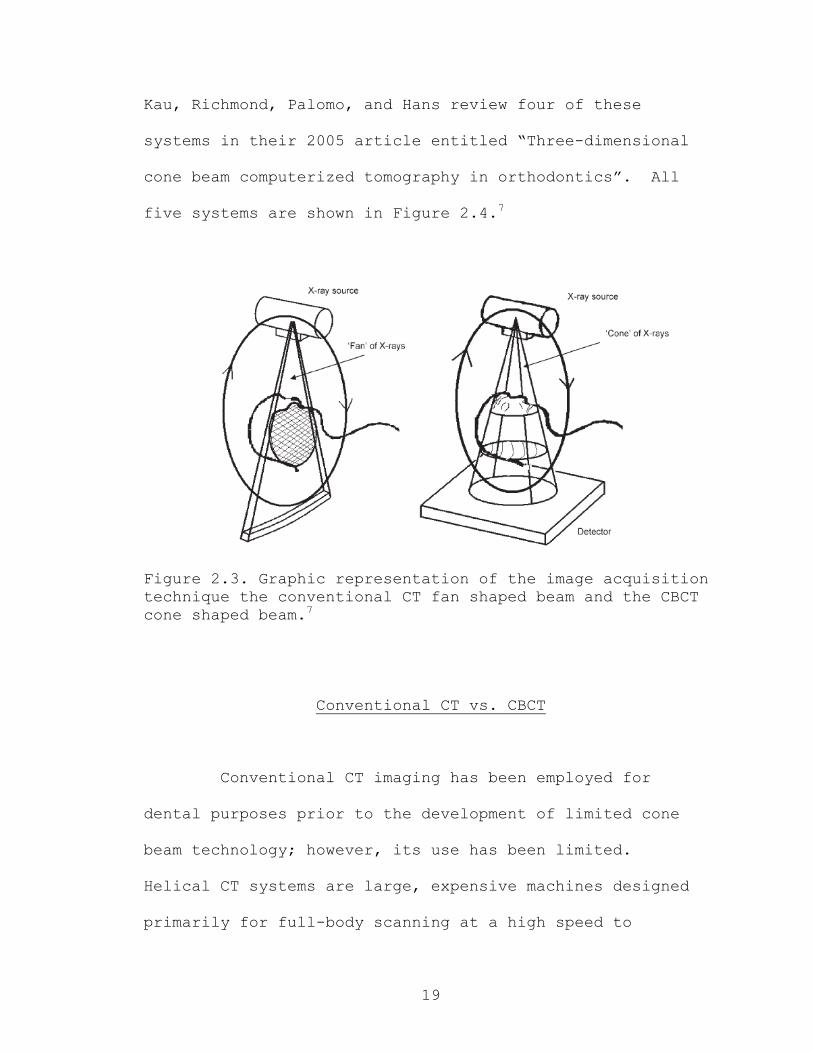
examined (see Figure 2.3).35 The 3DX machine, marketed by

Morita Corporation, has an exposure time of 17 seconds,

close to that of a panoramic exposure, and the radiation

dose is about 1/100 of the helical-CT.35 Many other

machines have been produced and marketed since the

introduction of the 3DX. Generally, most use the same

technology which involves a cone-shaped x-ray beam and an

image intensifying sensor that rotate around the subject

under observation. The i-CAT (Imaging Sciences

International, Hatfield, PA) and the Iluma (IMTEC imaging,

Ardmore, OK) CBCT systems, however, use amorphous silicon

flat panel image detectors capable of producing less image

noise than image intensifier tube/charge-coupled device

systems.37

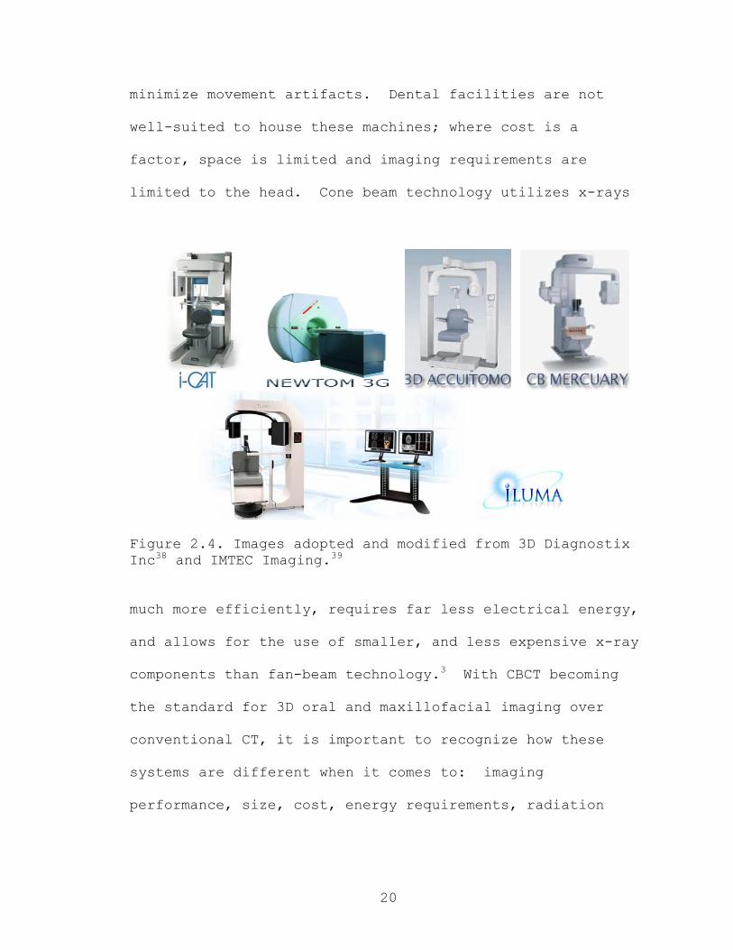
Some of the CBCT acquisition systems now available

on the world market7 include: the NewTom 3G by Quantitative

Radiology, the i-CAT by Imaging Sciences, the CB MercuRay

by Hitachi Medical, the 3D Accuitomo by J Morita

Manufacturing Corporation, and the Iluma by IMTEC imaging.

19

Kau, Richmond, Palomo, and Hans review four of these

systems in their 2005 article entitled “Three-dimensional

cone beam computerized tomography in orthodontics”. All

five systems are shown in Figure 2.4.7

Figure 2.3. Graphic representation of the image acquisition technique the conventional CT fan shaped beam and the CBCT cone shaped beam.7

Conventional CT vs. CBCT

Conventional CT imaging has been employed for

dental purposes prior to the development of limited cone

beam technology; however, its use has been limited.

Helical CT systems are large, expensive machines designed

primarily for full-body scanning at a high speed to

20

minimize movement artifacts. Dental facilities are not

well-suited to house these machines; where cost is a

factor, space is limited and imaging requirements are

limited to the head. Cone beam technology utilizes x-rays

Figure 2.4. Images adopted and modified from 3D Diagnostix Inc38 and IMTEC Imaging.39

much more efficiently, requires far less electrical energy,

and allows for the use of smaller, and less expensive x-ray

components than fan-beam technology.3 With CBCT becoming

the standard for 3D oral and maxillofacial imaging over

conventional CT, it is important to recognize how these

systems are different when it comes to: imaging

performance, size, cost, energy requirements, radiation

21

dosimetry, and the level of skill needed to operate the

systems.

Imaging Performance

A 2005 study by Holberg, Steinhäuser, Geis, and

Janson40 compared the image quality of fine dental

structures using both CBCT and conventional dental CT. The

CBCT imaging was carried out using the DVT-9000 (an earlier

version of the New Tom 3G), and conventional CT imaging was

accomplished using the Light Speed Ultra manufactured by

General Electric Company. Over 200 teeth were examined

with both systems; and image quality assessment was carried

out by three radiologically-experienced clinicians with a

minimum of five years experience in analyzing tomographic

slices of the craniofacial complex. The image quality of

the axial slices through the periodontal ligament space in

the root area was examined. The comparison between the two

systems was limited to axial slices which allows for the

production of high resolution images in conventional CT.33-35

The authors concluded that in contrast to dental CT, there

were little or no metal artifacts around fillings or

implants when CBCT was employed. A single metal filling

can render an entire axial slice with conventional CT

useless. They also found CBCT to be superior when it came

22

to the examination of major dental and skeletal structures

such as relation of teeth and visualization of skeletal

structures. However, when it came to examining fine

structures like the periodontal ligament space, enamel-

dentin interface, and the boundary of the pulp cavity, the

dental CT was superior.

Much of the difference in image quality of the axial

slices can be explained by the difference in acquisition

times. There was a difference of 77.9 seconds between CBCT

and the dental CT. With the longer acquisition time, CBCT

had a much greater chance of producing movement artifacts

that can affect the clarity of entire scan. With dental

CT, only the individual 1.1 second slice, in which the

movement occurred, will be affected. Many of the newer

CBCT machines have much shorter acquisition times ranging

from 10-40 seconds,7 therefore, likely to produce much fewer

movement artifacts than earlier machines.

Hashimoto et al. in 200636 also studied the imaging

performance of CBCT in comparison with helical CT. For the

study they employed the Asteion Super 4 edition (Toshiba,

Tokyo, Japan), a medical four-row multidetector CT (MDCT);

and the 3DX CBCT. In the United States and Europe the 3DX

is marketed as the 3D Accuitomo by Morita Company. The

purpose of this study was to evaluate the image quality of

23

3DX. To accomplish this they compared 3DX images with MDCT

images in order to determine how well bone and tooth

conditions could be reproduced. The subject of the study

was a dried right maxillary bone cut into eight slices 2 mm

thick toward the zygomatico-plate in parallel with the

midline plane. The slices were embedded in dental acrylic

resin at the level of the maxillary crowns; and returned to

their pre-cutting position prior to imaging. Slices were

imaged directly parallel to the median sagittal plane

corresponding to the direction in which the maxillary bone

had been cut. Acquisition time was 17 seconds for the 3DX,

and 0.75 seconds per slice for a total of 5.5 seconds for

the Asterion.

The examiners found image quality and bone slice

reproducibility to be far superior with the CBCT in

comparison to the MDCT. Reproducibility of the slices was

determined through visualization of bone trabeculae,

enamel, dentin, pulp cavity, periodontal ligament space,

and lamina dura. These structures were evaluated from

printed images produced from both machines, and compared

with the actual slices. Hashimoto et al. in 2003 showed

similar results in an earlier study when they compared

images of a maxillary central incisor and mandibular first

molar made with the same imaging systems. This evaluation

24

also focused on fine structures such as: cortical bone,

cancellous bone, enamel, dentin, pulp cavity, periodontal

ligament space, and lamina dura. The images made with the

3DX were evaluated as significantly higher in quality than

the corresponding MDCT images.34

It is important, in the interest of the current

study, to review the reliability of CBCT in the examination

of the TMJ bony anatomy. With helical CT being the

standard for evaluation of the TMJ bony components, it is

intuitive that it be used in a comparison to determine the

diagnostic reliability of CBCT. Honda, Larheim, Maruhashi,

Matsumoto, and Iwai did just this in their 2006 article:

“Osseous abnormalities of the mandibular condyle:

diagnostic reliability of cone beam computed tomography

compared with helical computed tomography based on autopsy

material”.6 The purpose of this study was to compare the

reliability of the 3DX with helical CT in detecting osseous

abnormalities of the mandibular condyle; using macroscopic

observation as the gold standard. The helical CT scanner

used was a Lemage SXE (GEYMS, Tokyo, Japan). Twenty-one

autopsy specimens were mounted in acrylic holders and

oriented according to clinical positioning for exposures

with the 3DX and helical CT. The 21 condyles were

independently assessed by two oral and maxillofacial

25

radiologists with 20 to 25 years experience. The condyles

were assessed for osseous abnormalities such as: cortical

erosion or osteophytosis and sclerosis.

Overall, the examiners found that the CBCT and

helical CT were both highly reliable for the evaluation of

the mandibular condyle. However, side-by-side, the CBCT

images were consistently of superior quality. None-the-

less, the experienced radiologists were able to accurately

diagnose abnormalities using either system. The authors

conclude that CBCT being much cheaper and with considerably

lower radiation dose in patients examinations, it is both a

cost effective and a dose effective way to examine the bony

components of the TMJ.

With respect to the literature reviewed, one could

conclude that CBCT is at least as if not more reliable than

helical CT in its imaging capabilities within the oral

maxillofacial complex.

Radiation Dosimetry

One of the greatest of advantages of the CBCT

scanner is its ability to produce high resolution

volumetric images with only a fraction of the radiation

required with helical CT scanners. This is accomplished

through the use of a cone shaped beam large enough to

26

capture the region of interest in one rotation. The beam

uses the x-ray emissions very efficiently,8 with less

scatter radiation than conventional CT,7 thereby reducing

the effective dose to the patient.8 Hashimoto et al. found

the exposure dose for the Asterion MDCT to be 400 times

greater than that for the 3DX. The measured skin dose per

examination was 1.19 mSv for 3DX and 458 mSv for MDCT.6

Mah, Danforth, Bumann, and Hatcher reported that the total

radiation absorbed for a CBCT scan is approximately 20%

that of a conventional CT scan.5

Ludlow, Davies-Ludlow, Brooks, and Howerton

evaluated the dosimetry of 3 CBCT devices: CB Mercuray,

NewTom 3G, and i-CAT.9 These devices were selected for

their capacity to perform 12 inch full field of view (FOV)

examinations. The 12 inch FOV permits imaging of the full

anatomic region used in craniometric calculations for

orthodontic diagnosis and treatment planning.

Termoluminescent dosemeters (TLDs) were placed in 24 sites

throughout the layers of a tissue-equivalent human skull

RANDO phantom. The locations of the sensors reflected

critical organs known to be sensitive to radiation.

Ludlow et al.9 found that the dose varied

substantially depending on the device. Effective doses

were derived from calculations in accordance with both

27

International Commission on Radiological Protection (ICRP)

1990 tissue weights and proposed 2005 tissue weights. The

effective doses in mSv were: NewTom 3G (45, 59), i-CAT

(135, 193), and CB Mercuray (477, 558). For the i-CAT

examination doses were 3 to 3.3 times greater than the

NewTom 3G; and the CB Mercuray was 10.7 to 9.5 greater than

the NewTom 3G. The FOV and various other factors play a

role in determining the radiation dosimetry. Some of these

include exposure settings such as kV, mA, and exposure

time. For the i-CAT these settings are fixed. The NewTom

3G, on the other hand, is capable of adjusting its mA

according to the size of the patient. The machine is able

to determine proper settings by taking a scout scan prior

to the main exposure. Lastly, the Mercuray is adjustable

at the discretion of the operator. The three systems

produced effective doses 4 to 42 times greater than

comparable panoramic examination doses (6.3 mSv, 13.3 mSv).9

Though the full FOV doses from the CBCT units used in this

study were 2-23% of comparable conventional CT examinations

reported in the literature,9 it is still important for the

clinician to recognize the fact that the radiation doses

are much greater than that of conventional radiography.

There is no question that CBCT imaging provides far

more undistorted, accurate information than conventional

28

radiography. However, unless the clinician is taking full

advantage of the added diagnostic capabilities in CBCT

examinations, they should consider using techniques that

expose the patient to less radiation in accordance with the

ALARA principle (As Low As Reasonably Achievable). Farman

and Scarfe41 suggest an imaging method which utilizes the

CBCT scout radiograph as 2D lateral cephalogram for

cephalometric analysis; and then using this information in

determining more specific regions requiring full 3D

renditions. A more focused FOV would minimize radiation

exposure to the patient. Chidiac, Shofer, Al-Kutoubi,

Laster and Ghafari42 also examined the possibility of

conventional CT scout radiographs being used for

cephalometric analysis. They found that CT scouts and

conventional cephalograms were close in angular

measurements, but differed in accuracy of imaging linear

measurements. They concluded that logistic and economic

considerations favor the use of conventional cephalograms.

It is important to take into account that these

considerations may not be as applicable with CBCT. As CBCT

technology progresses, exposure time and radiation dosages

are becoming less, and image quality is increasing.

29

Size and Cost

CBCT scanners are substantially lighter and smaller

than conventional CT scanners. They have no special

electrical requirements, no floor strengthening is

required, a there is no need for room cooling during

operation.38 Unlike CBCT, the conventional CT scanners do

not lend themselves to miniaturization because of the space

required for the fan shaped beam to spiral around the

entire body.3 The CBCT scanners are built specifically for

oral and maxillofacial imaging; and the FOV of the cone

beam allows the entire complex to be scanned in one

revolution. Thereby, allowing the CBCT to be more compact,

and therefore resulting in a smaller footprint requirement.

Because the head and neck can be adequately stabilized,

speed of the beam revolution is not as critical for CBCT as

it is for conventional CT. The conventional CT fan beam

must move at very high speeds in order to avoid artifacts

produced by movement of the heart, lungs, and bowels.3 The

mechanisms required to move the beam at high speeds while

at the same time moving the patient through the scanner,

can add significant cost to the design of the conventional

CT machine.3 Another factor that may cause a price

differential is that the use of a cone beam over a fan

beam, significantly increases x-ray utilization, thereby

30

reducing the x-ray tube heat capacity required for

volumetric scanning.3

CBCT Orthodontic Applications

Since the introduction of CBCT in the late 1990s,

it has become well established as an effective radiographic

tool for oral and maxillofacial diagnosis. CBCT is being

utilized for many of the same applications CT has been used

for in the past. However, with its improved

characteristics, such as lower radiation and improved

accessibility and affordability, it is being employed to a

much greater degree in orthodontic diagnosis and treatment

planning.

Accuracy

Cephalometric radiography has been the standard for

the assessment of skeletal, dental, and soft tissue

relationships since its development in the early 1900s.

Cephalometrics is used to describe craniofacial morphology,

evaluate growth, treatment plan, and evaluate treatment

results. One of the great shortcomings of the lateral

cephalogram is that it is a 2D representation of a 3D

structure. Two-dimensional images are not a good

31

representation of the patient’s 3D anatomic truth. No

individual’s face is completely symmetric; and the lack of

accurate superimposition of these asymmetric halves creates

error in landmark identification43 and skews cephalometric

measurements. Measurement error also results from the

magnification produced in conventional cephalometry. CT

and CBCT technology makes it possible to create

anatomically true (1:1 in size) images devoid of

magnification and superimposition. Apart from the error

that results from operator landmark identification,43 this

significantly reduces the error in linear and geometric

measurements.11,12 Enlow, in 2000, says this about the

future of cephalometric imaging: “The near-future will be

based on the actual biology of an individual’s own

craniofacial growth and development, and it will be

determined by a three-dimensional evaluation based on that

person’s actual morphogenic characteristics, not simply

developmentally irrelevant radiographic landmarks.”44 Both

the CT and CBCT are able to create accurate 3D

representations of the craniofacial complex, however; CT

has had little representation in orthodontic diagnosis and

treatment planning due to: high cost, elevated radiation,

and difficulty in image interpretation.

32

The accuracy of linear, geometric, and volumetric

measurements has been addressed by a number of

investigators. A 2004 study by Lascala, Panella, and

Marques evaluated the accuracy of the linear measurements

obtained in CBCT images with the NewTom 9000.11 Thirteen

internal and external measurements were made on eight dry

skulls with a digital caliper. These same measurements

were repeated in CBCT examinations and compared with the

real measurements. They found that all CBCT measurements

were slightly underestimated relative to the real

measurements, but only statistically significant at the

base of the skull. A possible explanation for the

measurement variability is that most of the measurements

were taken outside of the dentomaxillary area, which is the

region CBCT scanners are designed to image. Therefore, the

authors concluded that CBCT is reliable for linear

evaluation measurements of structures closely associated

with dental and maxillofacial imaging.11

Kobayashi, Shimoda, Nakagawa, and Yamamoto,45 also

investigated the accuracy of linear measurements with CBCT,

focusing on dentomaxillary structures alone. Both CBCT and

CT measurements were compared with actual digital caliper

measurements made on sliced cadaver mandibles. They found

that CBCT could be used to measure the distance between two

33

points in the mandible more accurately than with CT. The

measurement error was found to range from 0.01 to

0.65 mm on the CBCT and 0 to 1.11 mm for images produced by

the CT. The increased measurement error in the CT images

may be due to the loss of resolution of the system in the

direction of reformatting.45 Overall, it was concluded

that, CBCT proved to be a reliable tool for preoperative

evaluation before dental implant surgery due to its high

resolution, low cost, and low radiation.

It is also important to study the accuracy of CBCT

from a geometric point of view. Marmulla, Wörtche,

Mühling, and Hassfeld12 did just that in their 2005 article:

Geometric accuracy of the NewTom 9000 Cone Beam CT. They

found that the NewTom CBCT scanner could produce volume

tomograms whose geometric distortion was below the

resolution power of the volume tomograph. A maximum

deviation of 0.3 mm was determined from the 216

measurements performed on a polymethylmethacrylate block of

known dimensions.

The measurement accuracy of CBCT has been

investigated on an even smaller scale through the

evaluation of periodontal defects. Misch, Yi, and Sarment46

found that CBCT measurement were as equally useful for the

evaluation of interproximal defects as traditional methods:

34

periodontal probing and periapical radiographs. However,

CBCT has a distinct advantage over conventional periapical

radiographs in that it allows the clinician to accurately

evaluate the buccal and lingual bony defects as well.

With respect to the current study, it is important

to consider the capabilities of the CBCT to accurately

represent the TMJ in volumetric reconstructions. A recent

study by Hilgers, Scarfe, Scheetz, and Farman4 set out to

investigate the accuracy of CBCT TMJ measurements. The

purpose of the study was to develop CBCT MPR projections

that depict TMJ morphology and select mandibular

relationships, and then compare the reliability and

accuracy of CBCT measurements with conventional

cephalograms in three planes (lateral, posteroanterior, and

submentovertex). TMJ articulations of twenty-five dry

skulls were inspected using digital calipers for direct

measurements, and the imaging modalities mentioned above

for radiographic examination. They found that the i-CAT

CBCT accurately depicted the TMJ in all dimensions; and was

significantly more accurate than the conventional

cephalograms in all three orthogonal planes.

35

Impacted Teeth and Oral Abnormalities

Ectopic cuspids are a relatively common occurrence

the orthodontist must address. The ectopic or impacted

incidences of maxillary cuspids is only second to that of

the third molar; and has been reported by various authors

in ranges that fall between 0.92% and 3%.10,47 Impactions

are twice as common in females as in males.47 Maxillary

impactions are most often located palatally (85%);10 and of

the patients with maxillary impactions, approximately 8%

are bilateral.47 The prevalence of mandibular impactions

(0.35%)47 is much lower than that of maxillary impactions.

The first challenge in treating impacted or ectopic

cuspids is determining their location. The most common way

of identifying buccal-lingual position of an object has

been through the use of the buccal object rule; also known

as the tube shift technique or Clark’s rule. This is

accomplished by taking two or more radiographs at different

projection angles. The objects position is then identified

by the relative positions of two separate objects changing

as the projection angle changes. This method has proven to

be 92% accurate in identifying the location of impacted or

ectopically erupting maxillary cuspids.48 Another method is

to use two radiographs taken at right angles to each other

such as a periapical and occlusal film.

36

Not only do ectopically erupting cuspids lead to

impaction, but they can also lead to resorption of the

neighboring permanent teeth. In 1987 Ericson and Kurol48

reported a 0.7% prevalence of resorbed permanent incisors

due to ectopic eruption of maxillary cuspids. Most

reported numbers of resorptions are relatively low,

however, it has been suggested that they occur more often

than is generally assumed.49 This may be due to the method

of radiographic analysis used in these studies. Often, 2D

images are incapable of revealing adequate detail needed to

make these diagnoses. Much of this is due to the overlap

of the incisors by the ectopic canine.50

With the use of 3D imaging, Ericson and Kurol, in

2000,50 discovered that 93% of ectopically positioned

canines were in direct contact with the root of the

adjacent lateral incisor and 12% with the central incisor.

CT scanning substantially increased the detection of

incisor root resorptions. In fact, 48% of the subjects in

their study had resorption of maxillary incisors due to the

ectopic eruption of maxillary canines. In this same study

intraoral films and CT scans were compared for their

diagnostic abilities in revealing maxillary incisor

resorptions. The number of root resorptions on lateral

incisors increased by 53% with the use of the CT imaging

37

over intraoral radiographs.50 With this in mind, it becomes

important to consider the diagnostic advantages CT scanning

can afford the clinician in management of ectopic canines.

Though this technology has been available for some time, it

is seldom used due to issues related to cost, risk/benefit,

access, and expertise in reading the CT.10

The introduction of CBCT has made 3D imaging more

amenable for the evaluation of ectopic erupting and/or

impacted canines. A more recent study by Walker, Enciso,

and Mah10 supports the claims of incisor resorption

prevalence made in the previous study.50 For this study

CBCT was used instead of conventional CT; and it proved to

be equally effective in: locating maxillary ectopic

cuspids, defining their proximity to adjacent teeth, and

identifying and quantifying the extent of root resorption

caused by ectopic erupting canines.

CBCT can also be quite useful in the detection of

other oral abnormalities. Some clinicians across the USA

have begun to use CBCT in routine dental examination

procedures. Initial reports from these clinicians have

revealed a higher incidence of oral abnormalities than

previously suspected (i.e. oral cysts, ectopic/buried teeth

and supernumeraries).7 Kau et al. recommend that:

38

The value of these findings must be taken with caution, as the number of elective treatments that may be carried out may be limited. This leads to the question of whether to intervene in every abnormality located on these three-dimensional images and the extent to which the patient needs to be informed. In the event that these abnormalities were to lead to pathological episodes, what responsibilities would the clinician hold in the decision making process? This could lead to a host of future medico-legal problems on how clinicians and patients manage information.7

With the increasing availability and ever improving

technological capabilities, CBCT is becoming more and more

prevalent in the orthodontic office. With respect to the

above statement, the practicing clinician will have to make

the decision as to when it is appropriate to utilize this

technology; and when abnormalities are revealed in so

doing, what actions will they take, or will they be

expected to take in their management?

Airway Analysis

Evaluation of the upper airway can be accomplished

with a variety of different imaging modalities.

Historically, the most conventional means for the

orthodontist has been through the use of lateral

cephalograms. However, its diagnostic capabilities are

limited due to its inability to accurately represent the 3D

anatomy of the skeletal and soft tissue structures that

39

comprise the oral and nasopharyngeal airways. Proper

functionality of the airway relies on adequate volumes of

air to be allowed to pass through (airflow). One of the

main goals in airway evaluation is to define the volumetric

capabilities of the airway under observation. Lateral

cephalometric radiographs have no volumetric capabilities

to assist in this task. Conventional CT scans do have this

capacity; however, they typically demonstrate poor

resolution for upper airway adipose tissue when compared to

magnetic resonance imaging (MRI).

CBCT volumetric imaging abilities may also be

useful in the evaluation of the airway. With this being a

newer technology, few studies have been accomplished to

examine its capabilities in this aspect. Aboudara,

Hatcher, Nielsen, and Miller51 conducted a retrospective

cross-sectional chart review pilot study that evaluated the

2D airway from lateral cephalograms and 3D airway structure

from CBCT scans. They found that there was intra-subject

variation in the airway CT volume to lateral Cephalogram

area; and the variation was greater in airway volume than

airway area. They concluded that there may be airway

information that is not accurately depicted with the

lateral cephalogram and that more analysis with a greater

sample size is needed. In a more recent study CBCT was used

40

to evaluate volumetric changes that occur in the airway

following mandibular advancement or setback surgery.52

Contrary to what earlier studies using lateral cephalograms

have shown, CBCT examination did not reveal a significant

change in airway volume with advancement or setback

procedures.52 This difference in findings is likely due to

the inability of the lateral cephalogram to measure the

changes that occur in all directions as is possible with

CBCT.52

Orthognathic Surgery

Many of the applications of CBCT in conventional

orthodontics also apply in combined orthodontic-

orthognathic surgery treatments. In fact, 3D CT has

already been applied to a much greater extent in

maxillofacial surgery than in orthodontics. Conventional

CT has been widely used in surgical planning for

craniofacial malformations, acquired defects, skull base

abnormalities, head and neck cancer; it has also found its

place in the measurement of the volume of oral tumors,

analysis of primary nasal deformity in cleft lip and palate

infants, assessment of naso-orbitoethmoidal fractures, and

for the evaluation of airway changes as well as for in

vitro experimental validation of 3D landmark measurement in

41

craniofacial surgery planning.32 Conventional CT and CBCT

provide the surgeon with the ability to create Biomodels

through stereolithography or milling process. Biomodels

provide the surgeon with invaluable information to assist

in presurgical planning for orthognathic cases, traumatic

injury cases, as well as a variety of other applications.

Temporomandibular Joint Evaluation: Imaging

The summer of 1987 a Michigan jury awarded $850,000

in an orthodontic case.53 The plaintiff, a teenage female,

received routine orthodontic treatment to correct a Class

II Division 1 malocclusion with a 7 mm anterior open bite.

The patient was treated with two upper bicuspid extractions

and the use of headgear. The patient experienced no signs

or symptoms of temporomandibular disorder (TMD) prior to

treatment, but developed symptoms shortly after completion

of treatment. The expert witnesses for the plaintiff

agreed that the patient’s predilection for TMD should have

been identified prior to initiating orthodontic care, that

the extraction of bicuspids was contraindicated and was a

departure from the standard of acceptable orthodontic

practice.

42

Publicity of the court decision sparked great

interest in the relationship between orthodontic treatment

and TMD in the dental research community. Studies

conducted since and have demonstrated limited evidence of a

relationship between TMD and orthodontic treatment.54-56

Kim, Graber and Viana54 performed a meta-analysis of the

literature, using the evidence from 31 primary studies to

analyze and evaluate the relationship between orthodontic

treatment and TMD. The data from their meta-analysis

showed no indication that traditional orthodontic treatment

increased the prevalence of TMD. In another review of the

literature, Luther55 found that orthodontic treatment has

little role to play in worsening or precipitating TMD when

treated patients are compared with untreated individuals.

Studies suggest that orthodontic treatment is at worst, TMD

neutral.55

Despite the lack of evidence to establish a link

between orthodontic treatment and the incidence of TMD;

orthodontists must continue to be vigilant in their

pretreatment evaluations, make accurate TMJ diagnoses, and

be quick to respond when unanticipated joint problems

arise. A proper screening for TMJ health status requires a

thorough history, as well as comprehensive clinical and

43

radiographic examinations. TMJ radiographic examination

will be the focus for the purposes of the current study.

According to Okeson57 there are three limiting

conditions that must be considered prior interpretation of

TMJ radiographs: 1) Absence of articular surfaces, 2)

Superimposition of subarticular surfaces, and 3) Variations

in normal. 1) Absence of articular surfaces: The

articular surfaces of the condyle, disk, and fossa are made

of dense fibrous connective tissue standard radiographs

have no capacity to capture. Therefore, the surfaces of

the condyle and fossa viewed in standard radiographs are

actually subarticular bone. 2) Superimpositions of

subarticular surfaces: Apart from corrected tomograms and

CT scans, routine radiographic images of the TMJ preset

with superimpositions of subarticular surfaces, limiting

the application of these images. 3) Variations in normal:

Variation from what one considers normal TMJ morphology is

not always an indication of pathosis. The examiner must

take into account the great variation that exists from one

subject to another. One must also consider other factors

that may contribute such as radiographic technique and

patient positioning. Okeson57 recommends that radiographs

should not be used to diagnose TMJ disorder, but instead,

44

serve as additional information to support or negate an

already established clinical diagnosis.

2D Imaging

Various forms of imaging techniques can be used to

evaluate temporomandibular joint (TMJ) form and function.

Okeson57 suggests four basic radiographic techniques that

can be used in most general dental practices: the

panoramic, lateral transcranial, transpharyneal, and

transmaxillary anteroposterior (AP) views. Generally, in

orthodontic diagnosis and treatment planning, the panoramic

radiograph serves as an initial screening tool for TMJ

evaluation. Dixon30 suggests that in consideration of other

imaging techniques for detecting osseous abnormalities, the

panoramic radiograph is an excellent choice for a screening

view of the TMJ due to its cost effectiveness, high

availability, and relatively low radiation dose. However,

the diagnostic capability of panoramic radiographs is

limited to gross osseous changes.1 Only obvious erosions,

sclerosis, and osteophytes of the condyle can be

identified.1 It has limited use for the identification of

early lesions, and no capability to provide information on

joint soft tissue status.30

45

Conventional tomography may give the practitioner

more insight into the exact morphology of the osseous

structures of the TMJ. Generally it is accepted as being

superior to plane film radiography in the assessment of

joint spaces and the detection of osseous lesions of the

joint complex.30 Also, tomography has been shown to reveal

a greater number of structural changes, and represent

anatomic structures more accurately than transcranial

radiography.58-60 However, like the panoramic radiograph, it

has limited utility in the detection of early arthritic

changes; and even more advanced changes in the fossa tend

to go undetected.30 Dixon30 suggests that “this may explain

why radiographic findings often correlate poorly with

clinical signs and symptoms, which often peak early in the

disease”. Brookes et al.1 makes these final remarks about

conventional tomography:

Because conventional tomography has been used so often for years, it is relatively well studied. It is clear that there are few if any correlations between clinical and radiographic findings. Thus patients with radiographically normal joints may have pain, just as those with clear signs of bone abnormalities may be pain free. The value of radiographic evaluation lies in the ability of radiographs to help clinicians better understand the condition of the joint. Indeed, some studies have indicated that tomography can provide unanticipated information that may lead to a change in treatment plan. In contrast, however, other investigations have concluded that the presence or extent of radiographic signs of osseous pathoses are of little

46

prognostic value in the outcome of treatment and that tomography has little effect on the diagnosis or treatment plan of patients with TMJ disorders.

Similar to plane film radiography, conventional

tomography has little or no capacity to image soft tissue

structures within the joint space; nor can it reliably

predict articular disk position.1 Arthrography and

arthrotomography, contrast-enhanced plain or tomographic

radiography, augment the soft tissue imaging potential of

plane and tomographic radiography by introducing a

radiopaque contrast medium into the lower, upper, or both

joint space compartments. Often, the radiopaque medium is

injected under fluoroscopic guidance. Once contrast medium

injection is accomplished, plane films or tomograms can

then be obtained in the usual manner. The articular disk

appears as a radiolucent mass against a background of

contrast medium; thereby, providing information on disk

location, shape, and even movement with the use of video

fluoroscopy. Disk perforations, attachments, and or disk

adhesions and capsular tears may also be determined by flow

of contrast medium from one joint space compartment to

another.1

Arthrography is an excellent, mildly invasive

modality for radiographic evaluation of joint soft tissue

47

dynamics and internal joint derangements.30 However, there

are a number of disadvantages to Arthrography which include

but are not limited to: patient discomfort associated with

injection of contrast medium;30 true joint dynamics may be

disturbed by the presence of contrast medium;30 extensive

experience is required for such a technique sensitive

procedure;30 possible allergic reactions to the contrast

medium;1 and radiation exposure to the patient can be

significant, particularly with the use of fluoroscopy.1

Arthrography itself yields little information about the

osseous structures of the TMJ due to the presence of

radiopaque contrast medium.1 Therefore, another form of

imaging must be used in conjunction with arthrography in

order to evaluate the osseous and soft tissue structures.

3D Imaging

With CT and CBCT it is possible to image both hard

and soft tissues without the introduction of contrast

medium. Thereby, allowing the practitioner to assess the

disk-condyle relationship without disturbing the existing

anatomic relationship, or causing physical trauma to the

local tissues.57 Honda et al.61 recommend that air contrast

arthrography using CBCT is effective for diagnosis of disk

location, configuration, presence of adhesions and

48

perforations; and should be considered for cases of TMJ

disorder in the presence of contrast medium

contraindication or MRI contraindications. “Though some

early studies showed promise for CT in the detection of

internal derangement, magnetic resonance imaging (MRI) has

proven to demonstrate disk position and morphologic

condition better than CT and has almost completely

supplanted CT for this diagnostic purpose.”1 Today, MRI is

the preferred examination for TMJ soft tissue pathology.61

Dixon30 reports that several studies have assessed the

validity of MRI in diagnosing disk displacements and found

that the sensitivity in all studies was at least 0.86. One

study reported an accuracy that may reach as high as 95%.62

MRI has also been shown to be useful in the evaluation of

osseous lesions, and joint effusion; and shows potential as

a diagnostic aid for avascular necrosis of the condyle.30

One of the chief advantages of MRI over

radiographic techniques lies in the substitution of

superconducting magnets and radio wave energy for the well

know hazards of ionizing radiation.30 However, MRI is not

safe for everyone. The powerful magnetic fields produced

in the imaging process can have highly detrimental effects

on patients that have metal artifacts within their body,

49

such as: pace makers, intracranial vascular clips, and

metal particles in the eye or other vital structures.1

CT and CBCT are best suited for the evaluation of

osseous morphology.1 They serve well for the diagnosis of

bony abnormalities including fractures, dislocations,

arthritis, ankylosis, and neoplasia.1 They can also provide

accurate information on the position of the condyle within

the fossa in open and closed mouth conditions.63 The 1997

position paper of the American Academy of Oral and

Maxillofacial Radiology1 suggests that, because of its high

cost and radiation dose, CT of the TMJ be reserved for the

evaluation of foreign body giant cell reaction to silicon

or polytetrafluoroethylene sheet implants, suspected

tumors, ankylosis, and complex facial fractures. However,

since the introduction of cone-beam technology in 2000,

these contraindications have been greatly diminished. For

this reason one might consider using CBCT to evaluate

conditions of lesser severity. Some orthodontists have

already begun to use CBCT as a comprehensive radiographic

examination for diagnosis and treatment planning. In a

feature article from the American Association of Dental

Maxillofacial Radiographic Technicians, Way64 shares his

CBCT imaging protocols and viewing sequences for the

orthodontist. He also describes patient flow and

50

integration of CBCT into the orthodontic initial

examination process. CBCT viewing involves screening for

pathology, airway analysis, ectopically erupting as well as

impacted teeth, asymmetries, cephalometric analysis and TMJ

studies.64

A 2004 report by Tsiklakis, Syriopoulos and

Stamatakis63 describes a reconstruction technique for

radiographic examination of the TMJ using CBCT. The

technique results in obtaining lateral and coronal CBCT

images as well as 3D reconstructions of the TMJ. To assess

range and type of condylar movement a second scan was made

with the patient’s mouth open. This procedure was employed

for four case studies presented in the report. Tsiklakis

et al. concluded that the technique provided a complete

radiographic investigation of the bony components of the

TMJ, reconstructed images were of high diagnostic quality,

the scanning time and radiation dose were smaller than that

of conventional CT, and therefore, should be considered the

imaging modality of choice for the examination of bony

changes in the TMJ.

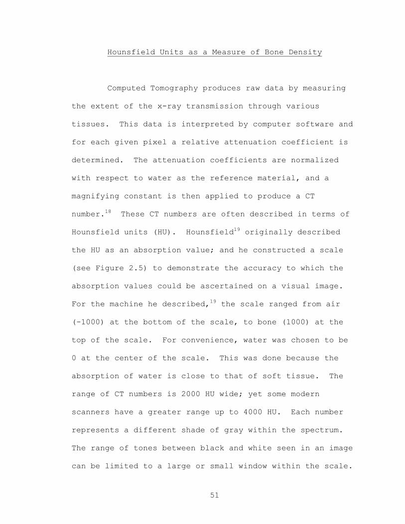
51

Hounsfield Units as a Measure of Bone Density

Computed Tomography produces raw data by measuring

the extent of the x-ray transmission through various

tissues. This data is interpreted by computer software and

for each given pixel a relative attenuation coefficient is

determined. The attenuation coefficients are normalized

with respect to water as the reference material, and a

magnifying constant is then applied to produce a CT

number.18 These CT numbers are often described in terms of

Hounsfield units (HU). Hounsfield19 originally described

the HU as an absorption value; and he constructed a scale

(see Figure 2.5) to demonstrate the accuracy to which the

absorption values could be ascertained on a visual image.

For the machine he described,19 the scale ranged from air

(-1000) at the bottom of the scale, to bone (1000) at the

top of the scale. For convenience, water was chosen to be

0 at the center of the scale. This was done because the

absorption of water is close to that of soft tissue. The

range of CT numbers is 2000 HU wide; yet some modern

scanners have a greater range up to 4000 HU. Each number

represents a different shade of gray within the spectrum.

The range of tones between black and white seen in an image

can be limited to a large or small window within the scale.

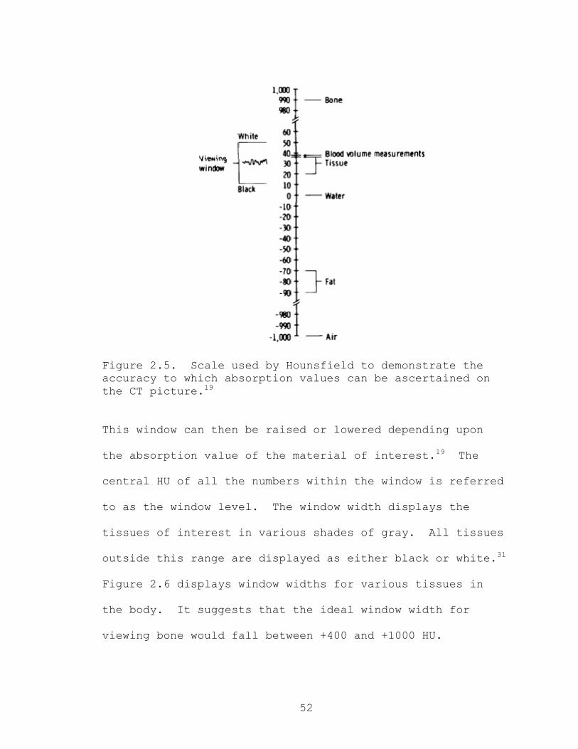
52

Figure 2.5. Scale used by Hounsfield to demonstrate the accuracy to which absorption values can be ascertained on the CT picture.19

This window can then be raised or lowered depending upon

the absorption value of the material of interest.19 The

central HU of all the numbers within the window is referred

to as the window level. The window width displays the

tissues of interest in various shades of gray. All tissues

outside this range are displayed as either black or white.31

Figure 2.6 displays window widths for various tissues in

the body. It suggests that the ideal window width for

viewing bone would fall between +400 and +1000 HU.

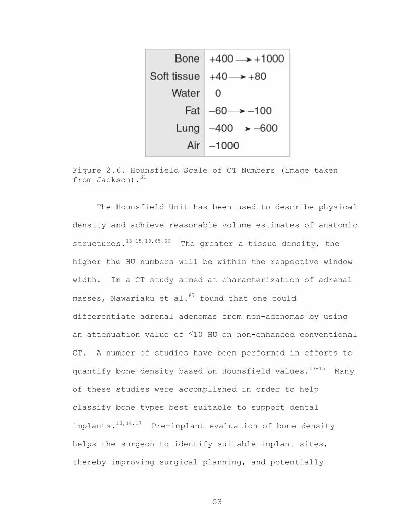
53

Figure 2.6. Hounsfield Scale of CT Numbers (image taken from Jackson).31

The Hounsfield Unit has been used to describe physical

density and achieve reasonable volume estimates of anatomic

structures.13-15,18,65,66 The greater a tissue density, the

higher the HU numbers will be within the respective window

width. In a CT study aimed at characterization of adrenal

masses, Nawariaku et al.67 found that one could

differentiate adrenal adenomas from non-adenomas by using

an attenuation value of ≤10 HU on non-enhanced conventional

CT. A number of studies have been performed in efforts to

quantify bone density based on Hounsfield values.13-15 Many

of these studies were accomplished in order to help

classify bone types best suitable to support dental

implants.13,14,17 Pre-implant evaluation of bone density

helps the surgeon to identify suitable implant sites,

thereby improving surgical planning, and potentially

54

improving implant success rates.13 Aranyarachkul et al.13

examined variations in bone density in designated implant

recipient sites using both CBCT and conventional CT. They

found both modalities to be consistent in their

measurements of bone density value; however, the values

were generally higher for CBCT. Whether CBCT or

conventional CT values are closer to corresponding

histological bone densities has yet to be investigated.

Yet, other studies have focused on relating CT

numbers not only to the density, but also the mechanical

properties of bone.15,16 Stoppie et al.15 and Rho et al.16

found that CT predictions of the mechanical properties in

bone were most accurate for specimens of full trabecular

bone, with little or no cortical bone present. For these,

a good correlation was found between the HU value and bone

mineral density (BMD). For jaws with a thicker cortical

layer the HU values were less reliable as predictors of

mechanical properties. Bone tissue density is a function

of both porosity and mineralization.16 Rho et al.16 suggest

that because such a poor correlation exists between CT

numbers and cortical bone density; and a much higher

correlation between CT numbers and cancellous bone density

is evident, it might be reasonable to consider CT numbers

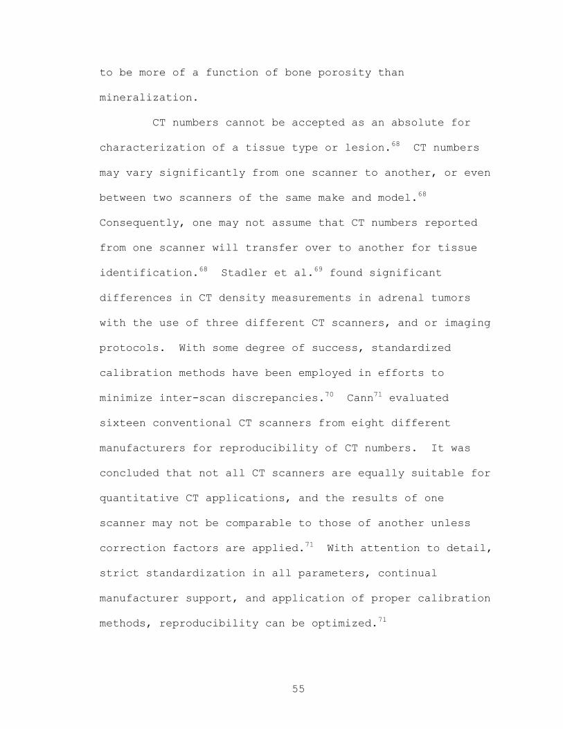
55

to be more of a function of bone porosity than

mineralization.

CT numbers cannot be accepted as an absolute for

characterization of a tissue type or lesion.68 CT numbers

may vary significantly from one scanner to another, or even

between two scanners of the same make and model.68

Consequently, one may not assume that CT numbers reported

from one scanner will transfer over to another for tissue

identification.68 Stadler et al.69 found significant

differences in CT density measurements in adrenal tumors

with the use of three different CT scanners, and or imaging

protocols. With some degree of success, standardized

calibration methods have been employed in efforts to

minimize inter-scan discrepancies.70 Cann71 evaluated

sixteen conventional CT scanners from eight different

manufacturers for reproducibility of CT numbers. It was

concluded that not all CT scanners are equally suitable for

quantitative CT applications, and the results of one

scanner may not be comparable to those of another unless

correction factors are applied.71 With attention to detail,

strict standardization in all parameters, continual

manufacturer support, and application of proper calibration

methods, reproducibility can be optimized.71

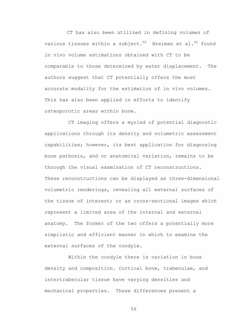
56

CT has also been utilized in defining volumes of

various tissues within a subject.66 Breiman et al.66 found

in vivo volume estimations obtained with CT to be

comparable to those determined by water displacement. The

authors suggest that CT potentially offers the most

accurate modality for the estimation of in vivo volumes.

This has also been applied in efforts to identify

osteoporotic areas within bone.

CT imaging offers a myriad of potential diagnostic

applications through its density and volumetric assessment

capabilities; however, its best application for diagnosing

bone pathosis, and or anatomical variation, remains to be

through the visual examination of CT reconstructions.

These reconstructions can be displayed as three-dimensional

volumetric renderings, revealing all external surfaces of

the tissue of interest; or as cross-sectional images which

represent a limited area of the internal and external

anatomy. The former of the two offers a potentially more

simplistic and efficient manner in which to examine the

external surfaces of the condyle.

Within the condyle there is variation in bone

density and composition. Cortical bone, trabeculae, and

intertrabecular tissue have varying densities and

mechanical properties. These differences present a

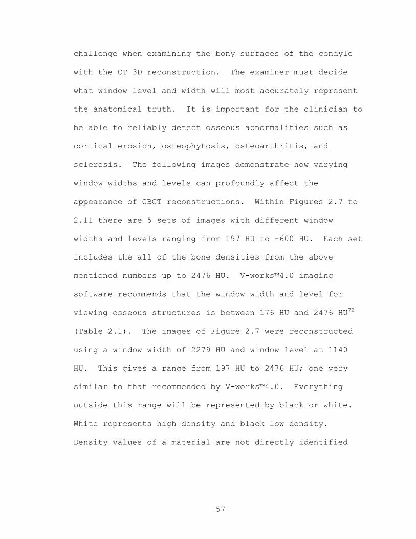
57

challenge when examining the bony surfaces of the condyle

with the CT 3D reconstruction. The examiner must decide

what window level and width will most accurately represent

the anatomical truth. It is important for the clinician to

be able to reliably detect osseous abnormalities such as

cortical erosion, osteophytosis, osteoarthritis, and

sclerosis. The following images demonstrate how varying

window widths and levels can profoundly affect the

appearance of CBCT reconstructions. Within Figures 2.7 to

2.11 there are 5 sets of images with different window

widths and levels ranging from 197 HU to -600 HU. Each set

includes the all of the bone densities from the above

mentioned numbers up to 2476 HU. V-works™4.0 imaging

software recommends that the window width and level for

viewing osseous structures is between 176 HU and 2476 HU72

(Table 2.1). The images of Figure 2.7 were reconstructed

using a window width of 2279 HU and window level at 1140

HU. This gives a range from 197 HU to 2476 HU; one very

similar to that recommended by V-works™4.0. Everything

outside this range will be represented by black or white.

White represents high density and black low density.

Density values of a material are not directly identified

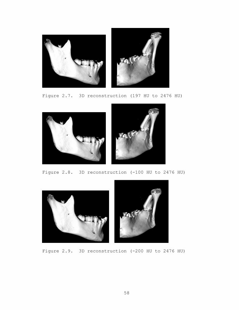
58

Figure 2.7. 3D reconstruction (197 HU to 2476 HU)

Figure 2.8. 3D reconstruction (-100 HU to 2476 HU)

Figure 2.9. 3D reconstruction (-200 HU to 2476 HU)

59

Figure 2.10. 3D reconstruction (-400 HU to 2476 HU)

Figure 2.11. 3D reconstruction (-600 HU to 2476 HU)

with Hounsfield units. For the V-works™ 4.0 imaging

software the density values start with the low density

value of air being at 0 and peak with a high density value

of 4095 for metal. In order to convert density values to

HU, one must simply subtract 1024 from the density value.72

Figure 2.12 reveals the photographic appearance of the

right condyle shown in the CBCT reconstructions of

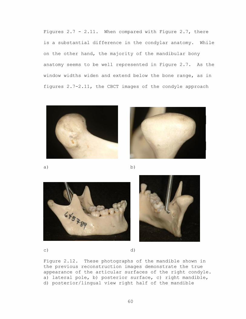
60

Figures 2.7 - 2.11. When compared with Figure 2.7, there

is a substantial difference in the condylar anatomy. While

on the other hand, the majority of the mandibular bony

anatomy seems to be well represented in Figure 2.7. As the

window widths widen and extend below the bone range, as in

figures 2.7-2.11, the CBCT images of the condyle approach

a) b)

c) d)

Figure 2.12. These photographs of the mandible shown in the previous reconstruction images demonstrate the true appearance of the articular surfaces of the right condyle. a) lateral pole, b) posterior surface, c) right mandible, d) posterior/lingual view right half of the mandible

61

Table 2.1. Window widths for density values and Hounsfield numbers in the body.72

a visual level closer to that of the photographic images.

Of the five reconstructions the -600 to 2476 gives the most

accurate representation of the bony articular anatomy. It

is likely that there is a greater range of densities within

the condyle when compared to the rest of the mandible, and

that it is heavily weighted on the low density end of the

scale. This presents a problem when examining the condyle

in vivo. These density ranges extend into the soft tissue

range; and the presence soft tissues begins to occlude

one’s capacity to view the osseous anatomy with the 3D

reconstruction. The purpose of the present study is to

investigate what the ideal Hounsfield unit values are for

the examination of the condyle; and if an ideal window

width and level can be identified, can one reliably

evaluate the mandibular condyle using the CBCT 3D

reconstruction?

62

References

1. Brooks SL, Brand JW, Gibbs SJ, Hollender L, Lurie AG, Omnell KA et al. Imaging of the temporomandibular joint: a position paper of the American Academy of Oral and Maxillofacial Radiology. Oral Surg Oral Med Oral Pathol Oral Radiol Endod 1997;83:609-618.

2. Quintero JC, Trosien A, Hatcher D, Kapila S. Craniofacial imaging in orthodontics: historical perspective, current status, and future developments. Angle Orthod 1999;69:491-506.

3. Sukovic P. Cone beam computed tomography in craniofacial imaging. Orthod Craniofac Res 2003;6 Suppl 1:31-36; discussion 179-182.

4. Hilgers ML, Scarfe WC, Scheetz JP, Farman AG. Accuracy of linear temporomandibular joint measurements with cone beam computed tomography and digital cephalometric radiography. Am J Orthod Dentofacial Orthop 2005;128:803-811.

5. Mah JK, Danforth RA, Bumann A, Hatcher D. Radiation absorbed in maxillofacial imaging with a new dental computed tomography device. Oral Surg Oral Med Oral Pathol Oral Radiol Endod 2003;96:508-513.

6. Honda K, Larheim TA, Maruhashi K, Matsumoto K, Iwai K. Osseous abnormalities of the mandibular condyle: diagnostic reliability of cone beam computed tomography compared with helical computed tomography based on an autopsy material. Dentomaxillofac Radiol 2006;35:152-157.

7. Kau CH, Richmond S, Palomo JM, Hans MG. Three-dimensional cone beam computerized tomography in orthodontics. J Orthod 2005;32:282-293.

8. Hatcher DC, Aboudara CL. Diagnosis goes digital. Am J Orthod Dentofacial Orthop 2004;125:512-515.

63

9. Ludlow JB, Davies-Ludlow LE, Brooks SL, Howerton WB. Dosimetry of 3 CBCT devices for oral and maxillofacial radiology: CB Mercuray, NewTom 3G and i-CAT. Dentomaxillofac Radiol 2006;35:219-226.

10. Walker L, Enciso R, Mah J. Three-dimensional localization of maxillary canines with cone-beam computed tomography. Am J Orthod Dentofacial Orthop 2005;128:418-423.

11. Lascala CA, Panella J, Marques MM. Analysis of the accuracy of linear measurements obtained by cone beam computed tomography (CBCT-NewTom). Dentomaxillofac Radiol 2004;33:291-294.

12. Marmulla R, Wortche R, Muhling J, Hassfeld S. Geometric accuracy of the NewTom 9000 Cone Beam CT. Dentomaxillofac Radiol 2005;34:28-31.

13. Aranyarachkul P, Caruso J, Gantes B, Schulz E, Riggs M, Dus I et al. Bone density assessments of dental implant sites: 2. Quantitative cone-beam computerized tomography. Int J Oral Maxillofac Implants 2005;20:416-424.

14. Shapurian T, Damoulis PD, Reiser GM, Griffin TJ, Rand WM. Quantitative evaluation of bone density using the Hounsfield index. Int J Oral Maxillofac Implants 2006;21:290-297.

15. Stoppie N, Pattijn V, Van Cleynenbreugel T, Wevers M, Vander Sloten J, Ignace N. Structural and radiological parameters for the characterization of jawbone. Clin Oral Implants Res 2006;17:124-133.

16. Rho JY, Hobatho MC, Ashman RB. Relations of mechanical properties to density and CT numbers in human bone. Med Eng Phys 1995;17:347-355.

17. Hatcher DC, Dial C, Mayorga C. Cone beam CT for pre-surgical assessment of implant sites. J Calif Dent Assoc 2003;31:825-833.

64

18. Mull RT. Mass estimates by computed tomography: physical density from CT numbers. AJR Am J Roentgenol 1984;143:1101-1104.

19. Hounsfield GN. Nobel Award address. Computed medical imaging. Med Phys 1980;7:283-290.

20. Crawford PR. 100 years of radiology: those early years. J Can Dent Assoc 1995;61:951-954.

21. Microsoft® Encarta® Online Encyclopedia, X Ray. http://encarta.msn.com/encyclopedia_761579196/X_Ray.html; 2006. Cited on August 30, 2006.

22. Jacobson PH, Fedran RJ. Making darkness visible: the discovery of X-ray and its introduction to dentistry. J Am Dent Assoc 1995;126:1359-1367.

23. Langland OE, Langlais RP. Early pioneers of oral and maxillofacial radiology. Oral Surg Oral Med Oral Pathol Oral Radiol Endod 1995;80:496-511.

24. Mupparapu M, Vuppalapati A. Detection of an early ossification of thyroid cartilage in an adolescent on a lateral cephalometric radiograph. Angle Orthod 2002;72:576-578.

25. Behrents R, Broadbent B, Jr. A Chronological Account of the Bolton-Brush Growth Studies; 1984.

26. Broadbent B, Jr. A New X-Ray Technique and Its Application to Orthodontia. The Angle Orthodontist 1931;1:2-24.

27. Hallikainen D. History of panoramic radiography. Acta Radiol 1996;37:441-445.

28. White S. Pharoah M. Oral Radiology Principles and Interpretation. St. Louis: Mosby; 2000.

65

29. Hendee WR. Cross sectional medical imaging: a history. Radiographics 1989;9:1155-1180.

30. Dixon DC. Radiographic diagnosis of temporomandibular disorders. Semin Orthod 1995;1:207-221.

31. Jackson ST, R. Cross-Sectional Imaging Made Easy. Edinburgh: Churchill Livingstone; 2004.

32. Papadopoulos MA, Christou PK, Christou PK, Athanasiou AE, Boettcher P, Zeilhofer HF et al. Three-dimensional craniofacial reconstruction imaging. Oral Surg Oral Med Oral Pathol Oral Radiol Endod 2002;93:382-393.

33. Nakajima A, Sameshima GT, Arai Y, Homme Y, Shimizu N, Dougherty H, Sr. Two- and three-dimensional orthodontic imaging using limited cone beam-computed tomography. Angle Orthod 2005;75:895-903.

34. Hashimoto K, Arai Y, Iwai K, Araki M, Kawashima S, Terakado M. A comparison of a new limited cone beam computed tomography machine for dental use with a multidetector row helical CT machine. Oral Surg Oral Med Oral Pathol Oral Radiol Endod 2003;95:371-377.

35. Araki K, Maki K, Seki K, Sakamaki K, Harata Y, Sakaino R et al. Characteristics of a newly developed dentomaxillofacial X-ray cone beam CT scanner (CB MercuRay): system configuration and physical properties. Dentomaxillofac Radiol 2004;33:51-59.

36. Hashimoto K, Kawashima S, Araki M, Iwai K, Sawada K, Akiyama Y. Comparison of image performance between cone-beam computed tomography for dental use and four-row multidetector helical CT. J Oral Sci 2006;48:27-34.

37. Baba R, Ueda K, Okabe M. Using a flat-panel detector in high resolution cone beam CT for dental imaging. Dentomaxillofac Radiol 2004;33:285-290.

66

38. 3D Diagnostix inc., Machine comparison chart. http://www.conebeam.com/cbct-clinician/manufacturers.php; 2006. Cited on March 12, 2006.

39. IMTEC Imaging, Product overview. http://www.ilumact.com/products.php; 2006. Cited on October 13.

40. Holberg C, Steinhauser S, Geis P, Rudzki-Janson I. Cone-beam computed tomography in orthodontics: benefits and limitations. J Orofac Orthop 2005;66:434-444.

41. Farman AG, Scarfe WC. Development of imaging selection criteria and procedures should precede cephalometric assessment with cone-beam computed tomography. Am J Orthod Dentofacial Orthop 2006;130:257-265.

42. Chidiac JJ, Shofer FS, Al-Kutoub A, Laster LL, Ghafari J. Comparison of CT scanograms and cephalometric radiographs in craniofacial imaging. Orthod Craniofac Res 2002;5:104-113.

43. Baumrind S, Frantz RC. The reliability of head film measurements. 1. Landmark identification. Am J Orthod 1971;60:111-127.

44. Enlow D. Discussion. Am J Orthod Dentofacial Orthop 2000;117:147.

45. Kobayashi K, Shimoda S, Nakagawa Y, Yamamoto A. Accuracy in measurement of distance using limited cone-beam computerized tomography. Int J Oral Maxillofac Implants 2004;19:228-231.

46. Misch KA, Yi ES, Sarment DP. Accuracy of cone beam computed tomography for periodontal defect measurements. J Periodontol 2006;77:1261-1266.

47. Bishara SE. Impacted maxillary canines: a review. Am J Orthod Dentofacial Orthop 1992;101:159-171.

67

48. Ericson S, Kurol J. Radiographic examination of ectopically erupting maxillary canines. Am J Orthod Dentofacial Orthop 1987;91:483-492.

49. Ericson S, Kurol J. Incisor resorption caused by maxillary cuspids. A radiographic study. Angle Orthod 1987;57:332-346.

50. Ericson S, Kurol PJ. Resorption of incisors after ectopic eruption of maxillary canines: a CT study. Angle Orthod 2000;70:415-423.

51. Aboudara CA, Hatcher D, Nielsen IL, Miller A. A three-dimensional evaluation of the upper airway in adolescents. Orthod Craniofac Res 2003;6 Suppl 1:173-175.

52. Stigall M. Oropharyngeal Airway Volume Changes: A Three-Dimensional Evaluation using Cone-Beam CT in Combined Orthodontic-Orthognathic Surgery Patients Orthodontics. St. Louis: Saint Louis University; 2006: p. 76.

53. Pollack B. Cases of note: Michigan jury awards $850,000 in ortho case: a tempest in a teapot. Am J Orthod Dentofacial Orthop 1988;94:358-360.

54. Kim MR, Graber TM, Viana MA. Orthodontics and temporomandibular disorder: a meta-analysis. Am J Orthod Dentofacial Orthop 2002;121:438-446.

55. Luther F. Orthodontics and the temporomandibular joint: where are we now? Part 1. Orthodontic treatment and temporomandibular disorders. Angle Orthod 1998;68:295-304.

56. Carlton KL, Nanda RS. Prospective study of posttreatment changes in the temporomandibular joint. Am J Orthod Dentofacial Orthop 2002;122:486-490.

57. Okeson J. Management of Temporomandibular Disorders and Occlusion. St. Louis: Mosby-Year Book, Inc.; 1993.

68

58. Eckerdal O, Lundberg M. The structural situation in temporomandibular joints. A comparison between conventional oblique transcranial radiographs, tomograms and histologic sections. Dentomaxillofac Radiol 1979;8:42-49.

59. Lindvall AM, Helkimo E, Hollender L, Carlsson GE. Radiographic examination of the temporomandibular joint. A comparison between radiographic findings and gross and microscopic morphologic observations. Dentomaxillofac Radiol 1976;5:24-32.

60. Bean LR, Omnell KA, Oberg T. Comparison between radiologic observations and macroscopic tissue changes in temporomandibular joints. Dentomaxillofac Radiol 1977;6:90-106.

61. Honda K, Matumoto K, Kashima M, Takano Y, Kawashima S, Arai Y. Single air contrast arthrography for temporomandibular joint disorder using limited cone beam computed tomography for dental use. Dentomaxillofac Radiol 2004;33:271-273.

62. Tasaki MM, Westesson PL. Temporomandibular joint: diagnostic accuracy with sagittal and coronal MR imaging. Radiology 1993;186:723-729.

63. Tsiklakis K, Syriopoulos K, Stamatakis HC. Radiographic examination of the temporomandibular joint using cone beam computed tomography. Dentomaxillofac Radiol 2004;33:196-201.

64. Way D. Utilization of CBCT in an Orthodontic Practice: AADMRT; 2006.

65. Kobayashi F, Ito J, Hayashi T, Maeda T. A study of volumetric visualization and quantitative evaluation of bone trabeculae in helical CT. Dentomaxillofac Radiol 2003;32:181-185.

69

66. Breiman RS, Beck JW, Korobkin M, Glenny R, Akwari OE, Heaston DK et al. Volume determinations using computed tomography. AJR Am J Roentgenol 1982;138:329-333.

67. Nwariaku FE, Champine J, Kim LT, Burkey S, O'Keefe G, Snyder WH, 3rd. Radiologic characterization of adrenal masses: the role of computed tomography--derived attenuation values. Surgery 2001;130:1068-1071.

68. Levi C, Gray JE, McCullough EC, Hattery RR. The unreliability of CT numbers as absolute values. AJR Am J Roentgenol 1982;139:443-447.

69. Stadler A, Schima W, Prager G, Homolka P, Heinz G, Saini S et al. CT density measurements for characterization of adrenal tumors ex vivo: variability among three CT scanners. AJR Am J Roentgenol 2004;182:671-675.

70. Cann CE. Quantitative CT for determination of bone mineral density: a review. Radiology 1988;166:509-522.

71. Cann CE. Quantitative CT applications: comparison of current scanners. Radiology 1987;162:257-261.

72. Cybermed. V-works™4.0. Seoul, Korea: Cybermed, co, Ltd; 2006: p. Imaging software for real time 3D visualization.

70

CHAPTER 3: JOURNAL ARTICLE

Abstract

Cone beam computed tomography (CBCT) has proven to

be a valuable imaging modality for examination of the

temporomandibular joint (TMJ). CBCT three-dimensional (3D)

reconstructions potentially provide the clinician with

efficient and effective means for evaluation of the

mandibular condyle. The purpose of the present study is to

investigate what the ideal Hounsfield unit values are for

the examination of the condyle; and if an ideal window

width and level can be identified, can one reliably

evaluate the mandibular condyle using the CBCT 3D

reconstruction?

Linear dimensions between six anatomical sights were

measured with a digital caliper to assess the anatomic

truth for 50 dry human mandibular condyles. Condyles were

scanned with the i-CAT (Imaging Sciences International,

Hatfield, PA) CBCT; and image reconstruction and assessment

was accomplished using V-works™4.0 (Cybermed Inc, Seoul,

Korea). Three linear three-dimensional measurements were

made on each of the 50 condyles at eight different

Hounsfield unit (HU) windows. These measurements were

71

compared with the anatomic truth. Volumetric measurements

were also completed on all 50 condyles, at 23 different

window levels, in order to define the volumetric

distribution of bone mineral density (BMD) within the

condyle. Significance testing for 3D linear measurement

and volumetric differences was accomplished using

independent t-tests with a 95% confidence interval.

Significant differences were found in two of the

three linear measurement groups at and below the

recommended viewing window for osseous structures. The

most accurate measurements were made within the soft tissue

range for HU window levels. Volumetric distribution

measurements revealed that the condyles were mostly

comprised of low density bone; and that condyles exhibiting

significant changes in linear measurements were shown to

have higher percentages of low density bone than those

condyles with little change from the anatomic truth.

Assessment of the mandibular condyle, using the 3D

reconstruction, is most accurate when accomplished at

density levels below that recommended for osseous

examination. Utilizing lower window levels, extending into

the soft tissue range, may compromise one’s capacity to

view the bony topography. This would suggest that CBCT 3D

reconstructed images, by themselves, may not be a reliable

72

means for the diagnosis condylar pathology, and or changes

in condylar morphology.

Introduction

Temporomandibular joint (TMJ) standard radiographic

studies such as the plain film radiography and panoramic

radiography have little capacity to reveal anything more

than gross osseous changes1 within the joint; and therefore,

in some cases a more comprehensive radiographic study is

indicated. Radiographic analysis of the TMJ is a broad

field and is considered by some to be a separate subset of

oral and maxillofacial radiology,2 consisting of both two

and three-dimensional imaging modalities. Two-dimensional

(2D) imaging of the TMJ employs conventional radiology to

produce a variety of projections. The submental-vertex,

lateral transcranial, transpharyneal, transmaxillary (AP),

as well as conventional tomography are a few examples of

the 2D studies used in TMJ evaluation. Three-dimensional

evaluations, such as computed tomography (CT) and magnetic

resonance imaging (MRI), have been utilized to some degree;

however, historically, high cost,3,4 large radiation

dosage,5,6 large space requirements,3,4 and the high level of

skill required for interpretation have kept its use to a

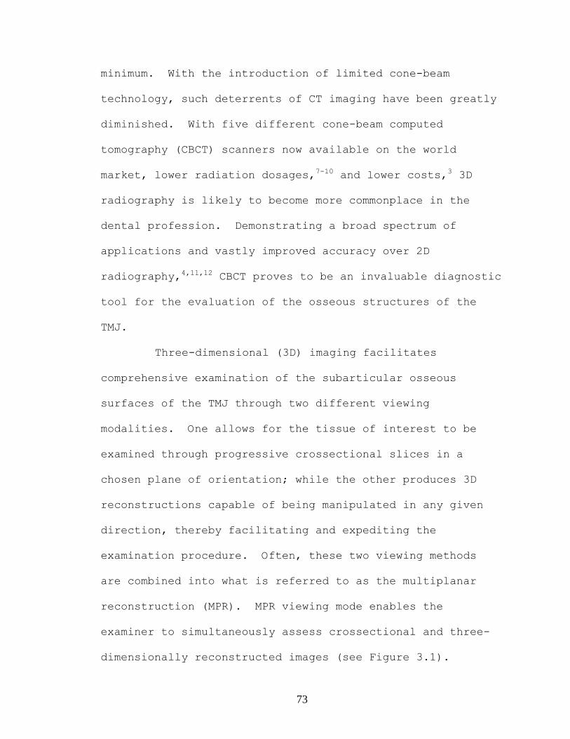
73

minimum. With the introduction of limited cone-beam

technology, such deterrents of CT imaging have been greatly

diminished. With five different cone-beam computed

tomography (CBCT) scanners now available on the world

market, lower radiation dosages,7-10 and lower costs,3 3D

radiography is likely to become more commonplace in the

dental profession. Demonstrating a broad spectrum of

applications and vastly improved accuracy over 2D

radiography,4,11,12 CBCT proves to be an invaluable diagnostic

tool for the evaluation of the osseous structures of the

TMJ.

Three-dimensional (3D) imaging facilitates

comprehensive examination of the subarticular osseous

surfaces of the TMJ through two different viewing

modalities. One allows for the tissue of interest to be

examined through progressive crossectional slices in a

chosen plane of orientation; while the other produces 3D

reconstructions capable of being manipulated in any given

direction, thereby facilitating and expediting the

examination procedure. Often, these two viewing methods

are combined into what is referred to as the multiplanar

reconstruction (MPR). MPR viewing mode enables the

examiner to simultaneously assess crossectional and three-

dimensionally reconstructed images (see Figure 3.1).

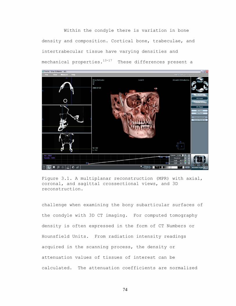
74

Within the condyle there is variation in bone

density and composition. Cortical bone, trabeculae, and

intertrabecular tissue have varying densities and

mechanical properties.13-17 These differences present a

Figure 3.1. A multiplanar reconstruction (MPR) with axial, coronal, and sagittal crossectional views, and 3D reconstruction.

challenge when examining the bony subarticular surfaces of

the condyle with 3D CT imaging. For computed tomography

density is often expressed in the form of CT Numbers or

Hounsfield Units. From radiation intensity readings

acquired in the scanning process, the density or

attenuation values of tissues of interest can be

calculated. The attenuation coefficients are normalized

75

with respect to water as the reference material, and a

magnifying constant is then applied to produce a CT

number.18 Hounsfield19 originally described the HU as an

absorption value; and he constructed a scale to demonstrate

the accuracy to which the absorption values could be

ascertained on a visual image. For the machine he

described,19 the scale ranged from air (-1000) at the bottom

of the scale, to bone (1000) at the top of the scale. Each

number represents a different shade of gray within the

spectrum. The range of tones between black and white seen

in an image can be limited to a large or small window

within the scale. This window can then be raised or

lowered depending upon the absorption value of the material

of interest.19 The examiner must be able to decide what

window level and width will most accurately represent the

anatomical truth of a tissue under examination. It is

important for the clinician to be able to reliably detect

osseous abnormalities such as cortical erosion,

osteophytosis, osteoarthritis, and sclerosis. The purpose

of the present study is to investigate what the ideal

Hounsfield unit values are for the examination of the

condyle; and if an ideal window width and level can be

identified, can one reliably evaluate the mandibular

condyle using the CBCT 3D reconstruction?

76

Materials and Methods

Selecting the Sample

The 25 dry human skulls in this study were used

with the permission of The Department of Anatomical

Science, Southern Illinois University at Edwardsville,

School of Dental Medicine. No demographic data were

available on the skulls such as age, gender, or ethnicity.

Each of the 50 condyles was inspected for any signs of wear

or abrasion and documented photographically. For each

condyle, six anatomic landmarks were identified, marked,

and photographed (see Figure 3.2).

Three linear measurements were made on the condyle

including: height, width, and length (see Table 3.2). All

direct measurements were made by one operator using an

electronic digital caliper (P.N. 50001, Chicago Brand,

Fremont, CA) with orthodontic tips. These measurements are

considered the “gold standard” (GS) for the purposes of

this study. Reproduction of the original landmark

locations on the 3D renderings was assisted through the use

of photographs and markings on the condyles themselves.

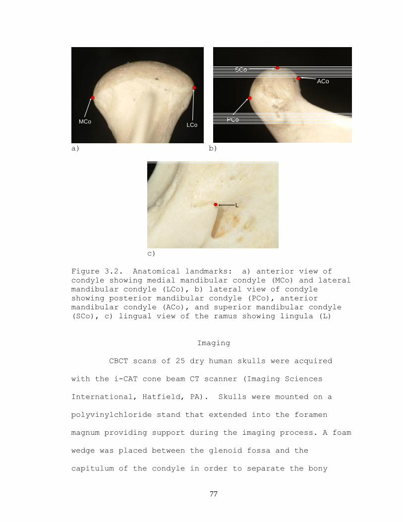
77

MCo LCo

PCo

ACo

SCo

a) b)

L

c) Figure 3.2. Anatomical landmarks: a) anterior view of condyle showing medial mandibular condyle (MCo) and lateral mandibular condyle (LCo), b) lateral view of condyle showing posterior mandibular condyle (PCo), anterior mandibular condyle (ACo), and superior mandibular condyle (SCo), c) lingual view of the ramus showing lingula (L)

Imaging

CBCT scans of 25 dry human skulls were acquired

with the i-CAT cone beam CT scanner (Imaging Sciences

International, Hatfield, PA). Skulls were mounted on a

polyvinylchloride stand that extended into the foramen

magnum providing support during the imaging process. A foam

wedge was placed between the glenoid fossa and the

capitulum of the condyle in order to separate the bony

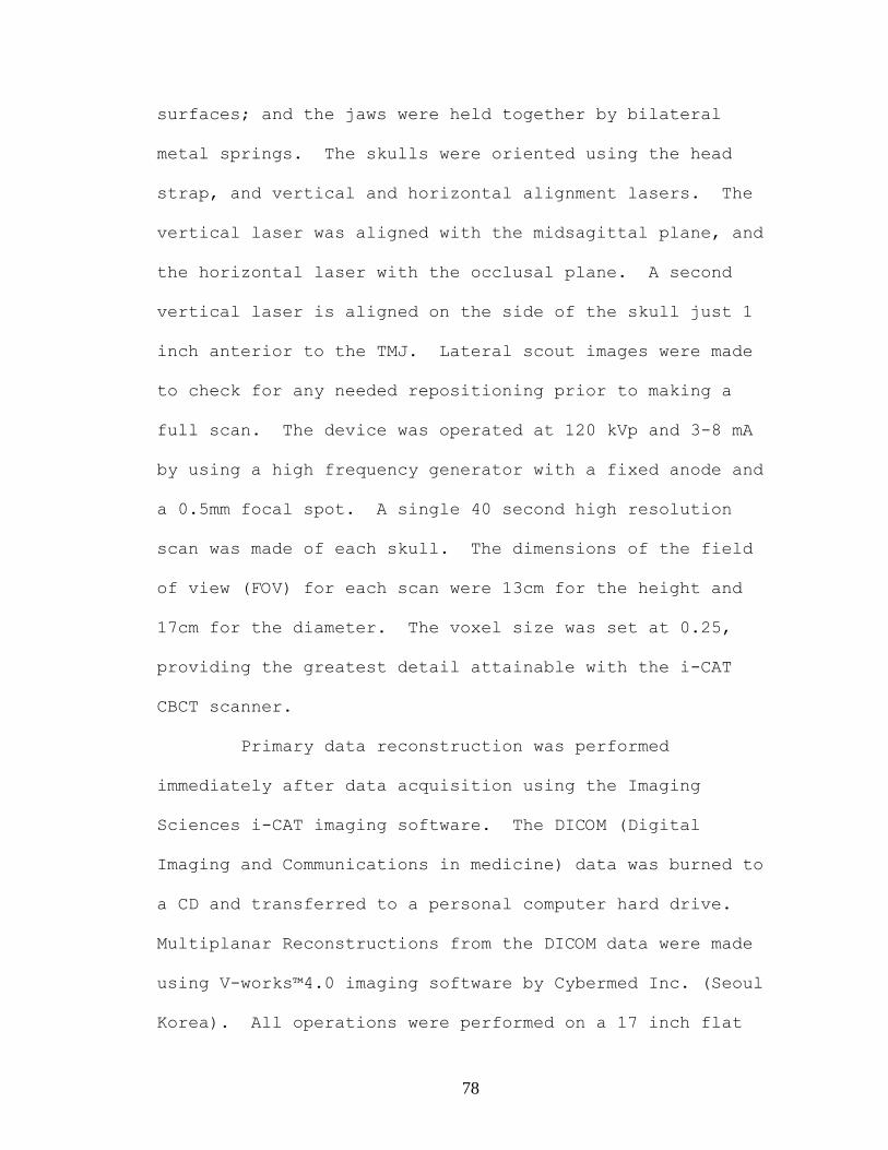
78

surfaces; and the jaws were held together by bilateral

metal springs. The skulls were oriented using the head

strap, and vertical and horizontal alignment lasers. The

vertical laser was aligned with the midsagittal plane, and

the horizontal laser with the occlusal plane. A second

vertical laser is aligned on the side of the skull just 1

inch anterior to the TMJ. Lateral scout images were made

to check for any needed repositioning prior to making a

full scan. The device was operated at 120 kVp and 3-8 mA

by using a high frequency generator with a fixed anode and

a 0.5mm focal spot. A single 40 second high resolution

scan was made of each skull. The dimensions of the field

of view (FOV) for each scan were 13cm for the height and

17cm for the diameter. The voxel size was set at 0.25,

providing the greatest detail attainable with the i-CAT

CBCT scanner.

Primary data reconstruction was performed

immediately after data acquisition using the Imaging

Sciences i-CAT imaging software. The DICOM (Digital

Imaging and Communications in medicine) data was burned to

a CD and transferred to a personal computer hard drive.

Multiplanar Reconstructions from the DICOM data were made

using V-works™4.0 imaging software by Cybermed Inc. (Seoul

Korea). All operations were performed on a 17 inch flat

79

panel WXGA TFT active matrix display (Toshiba USA) with a

screen resolution of 1440 X 900, and operated at 32 bit.

After importing the DICOM data into V-works™4.0, proper

steps were taken to create images needed for the study. To

do so, preset selection image options for the ‘head’ images

was selected, and the V-works™4.0 VR (Volume Rendering)

Preset ‘bone VR1’ was selected for the reconstruction.

Isolating and Measuring the Condyle

Each of the 50 condyles was isolated prior to

making the three-dimensional (3D) and volumetric

measurements. Frankfort Horizontal was constructed by

creating a line from the inferior orbital rim to the

superior boarder of the external auditory meatus. Using V-

works™4.0 volume operations and sculpting functions, an

initial cut was made parallel to Frankfort Horizontal just

above the superior aspect of the condyle, thereby removing

the majority of the surrounding bone. The remaining

surroundings were progressively removed using various V-

works™4.0 sculpting tools (see Figure 3.3).

Three-dimensional multiplanar reconstructions were

produced for each of the 8 window widths defined in Table

3.1. Reconstruction window width was set in the Volume

80

Table 3.1. Hounsfield Unit window widths (W) used to create 3D renderings of the condyles. 3D linear measurements were accomplished on each of these renderings.

Window Widths (W) for 3D Linear Measurements W1 -524 to 2476 HUW2 -424 to 2476 HUW3 -324 to 2476 HUW4 -224 to 2476 HUW5 -124 to 2476 HUW6 -24 to 2476 HUW7 76 to 2476 HUW8 176 to 2476 HU

mode using the histogram function. Once this was

accomplished, it was exported as a SOD (Selection on

Demand); and a 3D model was created in the MPR mode.

All 3D reconstruction linear measurements were made

using the point-to-point measuring function in the SSD

(shaded surface display) mode. The measurements include:

condylar width (CW), Condylar length (CL) and condylar

height (CH). CW is defined as the linear distance between

the most lateral aspect of the lateral pole to the most

medial point on the medial pole. CL is assessed by

measuring from the most posterior aspect of the condyle to

the most anterior point on the condylar head, and CH is

defined as the distance between the most superior point on

the condyle to the tip of the lingula. These landmarks and

the measurements made using them are defined in Tables 3.2

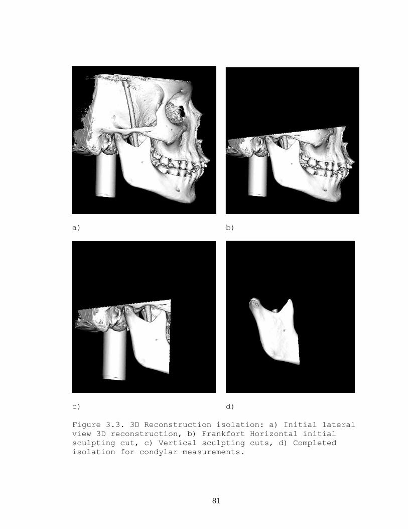
81

a) b)

c) d)

Figure 3.3. 3D Reconstruction isolation: a) Initial lateral view 3D reconstruction, b) Frankfort Horizontal initial sculpting cut, c) Vertical sculpting cuts, d) Completed isolation for condylar measurements.

82

and 3.3. The 3D measurements made are shown in Figure 3.4.

In the event of elimination of portions of condylar

anatomy due to variation in window widths virtual planes

are constructed in the SSD mode.

Table 3.2. Definitions of condylar linear measurements

Measurement Linear distance Definition

Condylar length (CL) ACo – PCo

Linear distance between anterior mandibular condyle and posterior mandibular condyle

Condylar width (CW) MCo – LCo

Linear distance between lateral mandibular condyle and medial mandibular condyle

Condylar height (CH) SCo - L Linear distance between superior

mandibular condyle and lingula

Table 3.3. Definitions of anatomic landmarks Landmark Definition

Anterior mandibular condyle (ACo)

Most anterior extent of the mandibular condyle viewed from the anterior, medial, lateral, and superior planes of view.

Posterior mandibular condyle (PCo)

Most posterior extent of the mandibular condyle viewed from the posterior, medial, lateral, and superior planes of view.

Lateral mandibular condyle (LCo)

Most lateral extent of the mandibular condyle viewed from the anterior, posterior, lateral, and superior planes of view.

Medial mandibular condyle (MCo)

Most medial extent of the mandibular condyle viewed from the anterior, posterior, medial, and superior planes of view.

Superior mandibular condyle (SCo)

Most superior aspect of the mandibular condyle viewed from the anterior, posterior, medial, lateral, and superior planes of view.

Lingula (L) Apex of the lingula

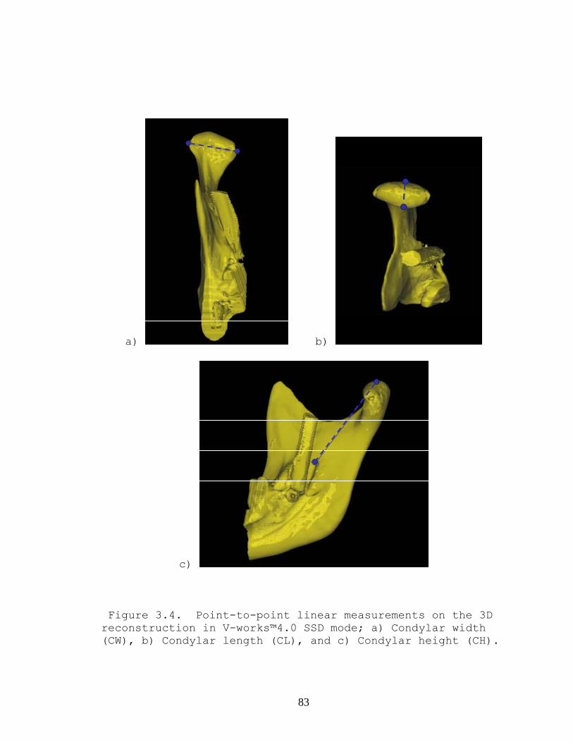
83

a) b)

c)

Figure 3.4. Point-to-point linear measurements on the 3D reconstruction in V-works™4.0 SSD mode; a) Condylar width (CW), b) Condylar length (CL), and c) Condylar height (CH).

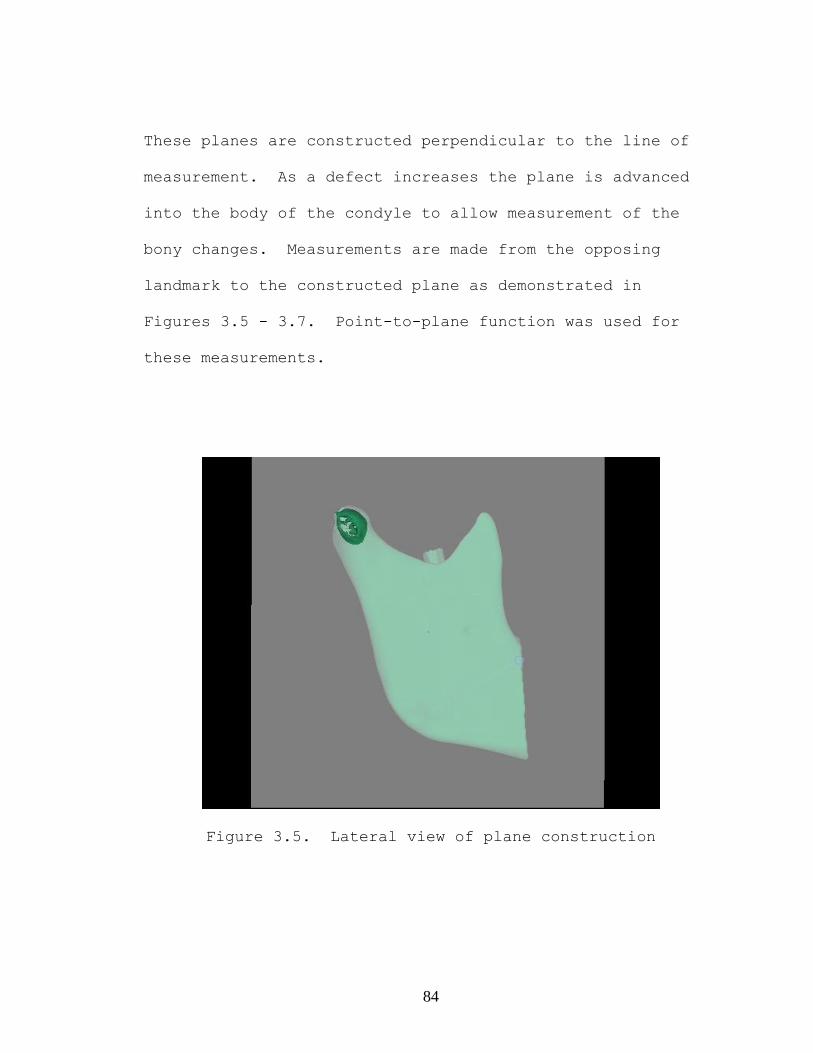
84

These planes are constructed perpendicular to the line of

measurement. As a defect increases the plane is advanced

into the body of the condyle to allow measurement of the

bony changes. Measurements are made from the opposing

landmark to the constructed plane as demonstrated in

Figures 3.5 - 3.7. Point-to-plane function was used for

these measurements.

Figure 3.5. Lateral view of plane construction

85

Figure 3.6. Superior view of plane construction

Figure 3.7. Anterior view of plane construction with (CW) measurement

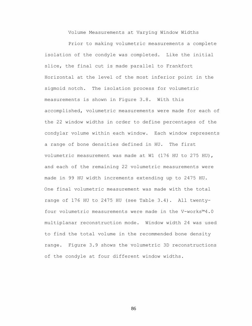
86

Volume Measurements at Varying Window Widths

Prior to making volumetric measurements a complete

isolation of the condyle was completed. Like the initial

slice, the final cut is made parallel to Frankfort

Horizontal at the level of the most inferior point in the

sigmoid notch. The isolation process for volumetric

measurements is shown in Figure 3.8. With this

accomplished, volumetric measurements were made for each of

the 22 window widths in order to define percentages of the

condylar volume within each window. Each window represents

a range of bone densities defined in HU. The first

volumetric measurement was made at W1 (176 HU to 275 HU),

and each of the remaining 22 volumetric measurements were

made in 99 HU width increments extending up to 2475 HU.

One final volumetric measurement was made with the total

range of 176 HU to 2475 HU (see Table 3.4). All twenty-

four volumetric measurements were made in the V-works™4.0

multiplanar reconstruction mode. Window width 24 was used

to find the total volume in the recommended bone density

range. Figure 3.9 shows the volumetric 3D reconstructions

of the condyle at four different window widths.

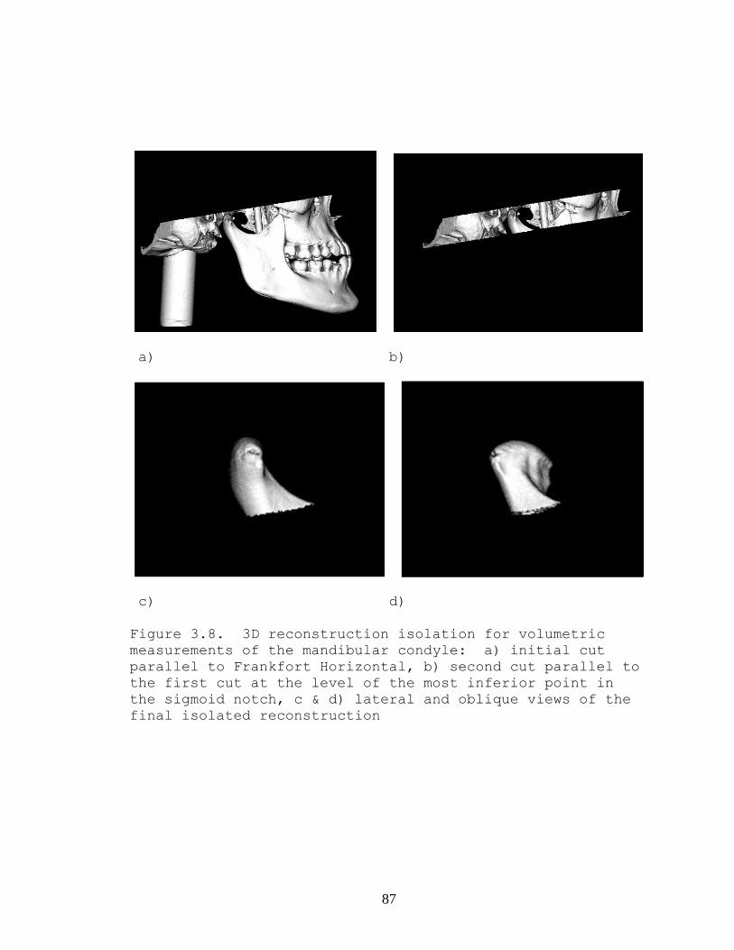
87

a) b)

c) d)

Figure 3.8. 3D reconstruction isolation for volumetric measurements of the mandibular condyle: a) initial cut parallel to Frankfort Horizontal, b) second cut parallel to the first cut at the level of the most inferior point in the sigmoid notch, c & d) lateral and oblique views of the final isolated reconstruction

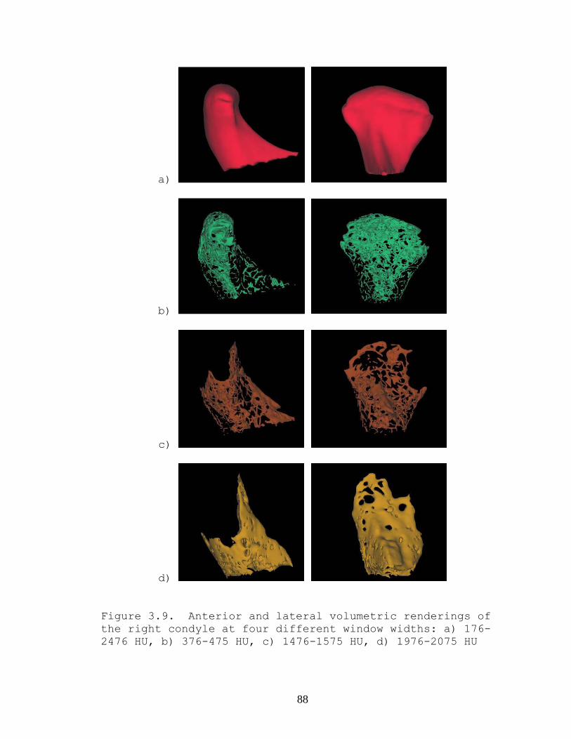
88

a)

b)

c)

d)

Figure 3.9. Anterior and lateral volumetric renderings of the right condyle at four different window widths: a) 176-2476 HU, b) 376-475 HU, c) 1476-1575 HU, d) 1976-2075 HU

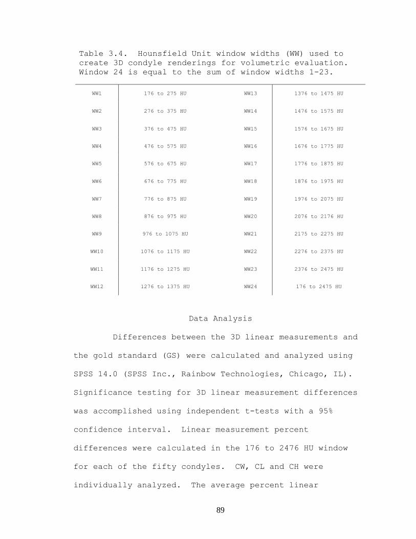
89

Table 3.4. Hounsfield Unit window widths (WW) used to create 3D condyle renderings for volumetric evaluation. Window 24 is equal to the sum of window widths 1-23.

WW1 176 to 275 HU WW13 1376 to 1475 HU

WW2 276 to 375 HU WW14 1476 to 1575 HU

WW3 376 to 475 HU WW15 1576 to 1675 HU

WW4 476 to 575 HU WW16 1676 to 1775 HU

WW5 576 to 675 HU WW17 1776 to 1875 HU

WW6 676 to 775 HU WW18 1876 to 1975 HU

WW7 776 to 875 HU WW19 1976 to 2075 HU

WW8 876 to 975 HU WW20 2076 to 2176 HU

WW9 976 to 1075 HU WW21 2175 to 2275 HU

WW10 1076 to 1175 HU WW22 2276 to 2375 HU

WW11 1176 to 1275 HU WW23 2376 to 2475 HU

WW12 1276 to 1375 HU WW24 176 to 2475 HU

Data Analysis

Differences between the 3D linear measurements and

the gold standard (GS) were calculated and analyzed using

SPSS 14.0 (SPSS Inc., Rainbow Technologies, Chicago, IL).

Significance testing for 3D linear measurement differences

was accomplished using independent t-tests with a 95%

confidence interval. Linear measurement percent

differences were calculated in the 176 to 2476 HU window

for each of the fifty condyles. CW, CL and CH were

individually analyzed. The average percent linear

90

measurement change was calculated for the fifty condyles in

each measurement group. All percent changes were plotted

on a distribution curve above and below the calculated

means for CW and CL. The mean percent change was 18.38 for

CL and 15.93 for CW. The distribution of numbers was

segmented into the following groups: 1) numbers < 10% fall

into groups CW0 and CL0; 2) the mean group included numbers

in the 10-24% range; and 3) numbers >24% in groups CW1 and

CL1. The mean group range of condyles was excluded from

the remainder of data analysis. The distribution of

condyles in their perspective ranges are shown in Figure

3.10. The percent volumes of the condyles in the outlying

groups were compared using independent t-tests at each of

the twenty-three volumetric window widths (WW) (see Table

3.5). The CL0 and CL1 groups were plotted on a

distribution curve to compare the distribution of bone

volume in the two groups (see Figure 3.11). The same was

done for the CW0 and CW1 groups on a separate graph (see

Figure 3.12). Linear measurement error was calculated by

using the interclass correlation coefficient on the 12

repeat measurements for CL, CW, and CH.

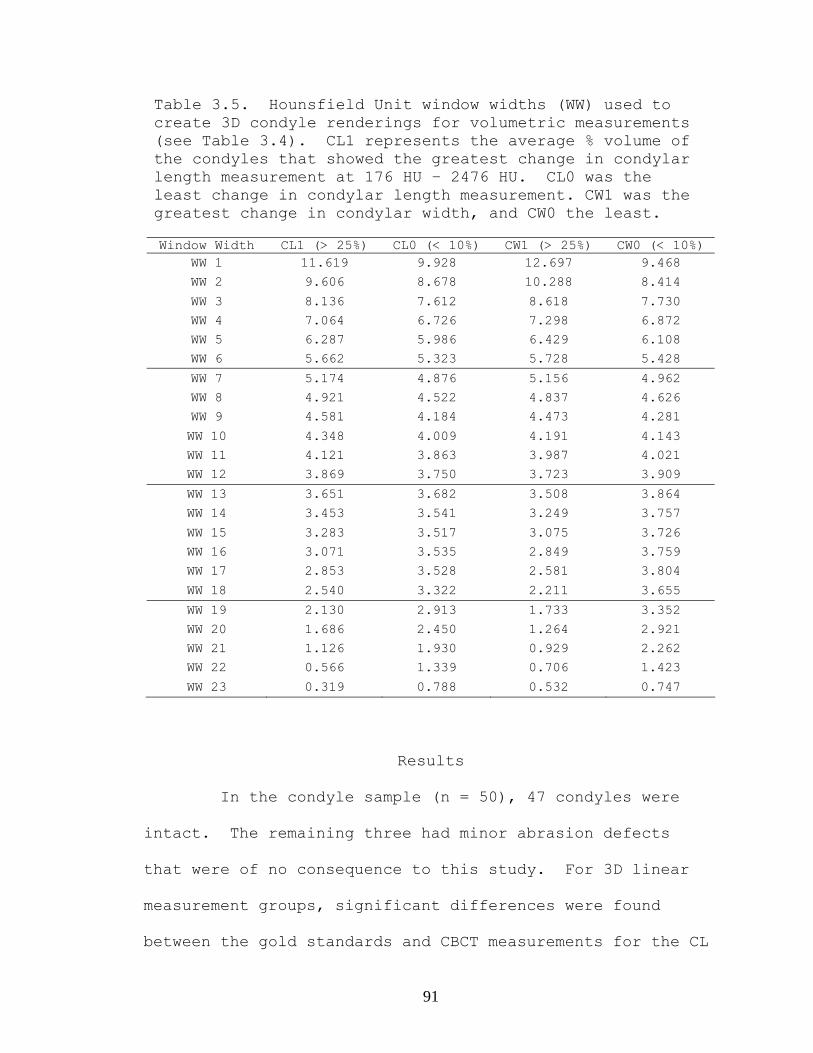
91

Table 3.5. Hounsfield Unit window widths (WW) used to create 3D condyle renderings for volumetric measurements (see Table 3.4). CL1 represents the average % volume of the condyles that showed the greatest change in condylar length measurement at 176 HU – 2476 HU. CL0 was the least change in condylar length measurement. CW1 was the greatest change in condylar width, and CW0 the least. Window Width CL1 (> 25%) CL0 (< 10%) CW1 (> 25%) CW0 (< 10%)

WW 1 11.619 9.928 12.697 9.468 WW 2 9.606 8.678 10.288 8.414

WW 3 8.136 7.612 8.618 7.730 WW 4 7.064 6.726 7.298 6.872 WW 5 6.287 5.986 6.429 6.108 WW 6 5.662 5.323 5.728 5.428

WW 7 5.174 4.876 5.156 4.962 WW 8 4.921 4.522 4.837 4.626 WW 9 4.581 4.184 4.473 4.281

WW 10 4.348 4.009 4.191 4.143 WW 11 4.121 3.863 3.987 4.021 WW 12 3.869 3.750 3.723 3.909

WW 13 3.651 3.682 3.508 3.864 WW 14 3.453 3.541 3.249 3.757

WW 15 3.283 3.517 3.075 3.726 WW 16 3.071 3.535 2.849 3.759 WW 17 2.853 3.528 2.581 3.804

WW 18 2.540 3.322 2.211 3.655

WW 19 2.130 2.913 1.733 3.352 WW 20 1.686 2.450 1.264 2.921 WW 21 1.126 1.930 0.929 2.262 WW 22 0.566 1.339 0.706 1.423

WW 23 0.319 0.788 0.532 0.747

Results

In the condyle sample (n = 50), 47 condyles were

intact. The remaining three had minor abrasion defects

that were of no consequence to this study. For 3D linear

measurement groups, significant differences were found

between the gold standards and CBCT measurements for the CL

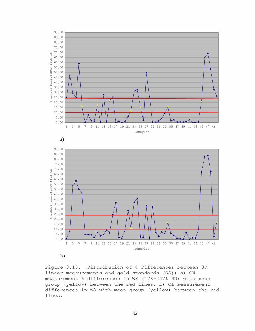
92

0.00

5.00

10.00

15.00

20.00

25.00

30.00

35.00

40.00

45.00

50.00

55.00

60.00

65.00

70.00

75.00

80.00

85.00

90.00

1 3 5 7 9 11 13 15 17 19 21 23 25 27 29 31 33 35 37 39 41 43 45 47 49

Condyles

% Linear Difference from GS

a)

0.00

5.00

10.00

15.00

20.00

25.00

30.00

35.00

40.00

45.00

50.00

55.00

60.00

65.00

70.00

75.00

80.00

85.00

90.00

1 3 5 7 9 11 13 15 17 19 21 23 25 27 29 31 33 35 37 39 41 43 45 47 49

Condyles

% Linear Difference From GS

b) Figure 3.10. Distribution of % Differences between 3D linear measurements and gold standards (GS); a) CW measurement % differences in W8 (176-2476 HU) with mean group (yellow) between the red lines, b) CL measurement differences in W8 with mean group (yellow) between the red lines.

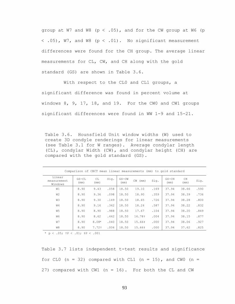
93

group at W7 and W8 (p < .05), and for the CW group at W6 (p

< .05), W7, and W8 (p < .01). No significant measurement

differences were found for the CH group. The average linear

measurements for CL, CW, and CH along with the gold

standard (GS) are shown in Table 3.6.

With respect to the CL0 and CL1 groups, a

significant difference was found in percent volume at

windows 8, 9, 17, 18, and 19. For the CW0 and CW1 groups

significant differences were found in WW 1-9 and 15-21.

Table 3.6. Hounsfield Unit window widths (W) used to create 3D condyle renderings for linear measurements (see Table 3.1 for W ranges). Average condylar length (CL), condylar Width (CW), and condylar height (CH) are compared with the gold standard (GS).

Comparison of CBCT mean linear measurements (mm) to gold standard

Linear measurement

Windows

GS-CL (mm)

CL (mm)

Sig.

GS-CW (mm) CW (mm) Sig. GS-CH

(mm) CH

(mm) Sig.

W1 8.90 9.43 .058 18.50 19.10 .169 37.94 38.66 .590

W2 8.90 9.36 .098 18.50 18.90 .359 37.94 38.39 .736

W3 8.90 9.30 .149 18.50 18.65 .726 37.94 38.28 .800

W4 8.90 9.16 .342 18.50 18.24 .587 37.94 38.22 .832

W5 8.90 8.90 .988 18.50 17.67 .104 37.94 38.20 .849

W6 8.90 8.62 .442 18.50 16.78† .004 37.94 38.15 .877

W7 8.90 8.08* .040 18.50 15.66‡ .000 37.94 38.06 .927

W8 8.90 7.72† .006 18.50 15.66‡ .000 37.94 37.62 .825

* p < .05; †P < .01; ‡P < .001

Table 3.7 lists independent t-test results and significance

for CL0 (n = 32) compared with CL1 (n = 15), and CW0 (n =

27) compared with CW1 (n = 16). For both the CL and CW

94

groups, the mean bone percent volume distribution was

greatest in the low density windows and lowest in the high

density windows (see Figures 3.11 and 3.12). CL0 and CW0

groups demonstrated greater percent volumes in the higher

density windows than the corresponding CL1 and CW1 groups.

Table 3.7. Comparison (Independent t-tests) of volumetric measurements: CL0 vs. CL1, and CW0 vs. CW1 at twenty-three window levels.

CL0 vs. CL1 CW0 vs. CW1

Volumetric Window t Sig. t Sig.

WW 1 -1.682 .100 3.417 .001† WW 2 -1.386 .173 2.925 .006† WW 3 -1.152 .255 2.637 .012* WW 4 -1.072 .289 2.165 .036* WW 5 -1.309 .197 2.489 .017* WW 6 -1.707 .095 2.697 .010* WW 7 -1.626 .111 2.265 .029* WW 8 -2.247 .030* 2.296 .027* WW 9 -2.358 .023* 2.211 .033* WW 10 -1.972 .055 1.197 .238 WW 11 -1.597 .117 .690 .494 WW 12 -.742 .462 -.246 .807 WW 13 .174 .863 -1.154 .255 WW 14 .435 .665 -1.819 .076 WW 15 1.044 .302 -2.350 .024* WW 16 1.812 .077 -3.287 .002† WW 17 2.323 .025* -4.210 .000‡ WW 18 2.323 .025* -4.333 .000‡ WW 19 2.091 .042* -4.403 .000‡ WW 20 1.861 .069 -4.133 .000‡ WW 21 2.038 .047* -3.292 .002† WW 22 2.288 .027* -1.909 .063

WW 23 1.543 .130 -.586 .561

* p < .05; †P < .01; ‡P < .001

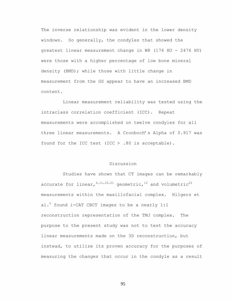
95

The inverse relationship was evident in the lower density

windows. So generally, the condyles that showed the

greatest linear measurement change in W8 (176 HU - 2476 HU)

were those with a higher percentage of low bone mineral

density (BMD); while those with little change in

measurement from the GS appear to have an increased BMD

content.

Linear measurement reliability was tested using the

intraclass correlation coefficient (ICC). Repeat

measurements were accomplished on twelve condyles for all

three linear measurements. A Cronboch’s Alpha of 0.917 was

found for the ICC test (ICC > .80 is acceptable).

Discussion

Studies have shown that CT images can be remarkably

accurate for linear,4,11,20,21 geometric,12 and volumetric22

measurements within the maxillofacial complex. Hilgers et

al.4 found i-CAT CBCT images to be a nearly 1:1

reconstruction representation of the TMJ complex. The

purpose to the present study was not to test the accuracy

linear measurements made on the 3D reconstruction, but

instead, to utilize its proven accuracy for the purposes of

measuring the changes that occur in the condyle as a result

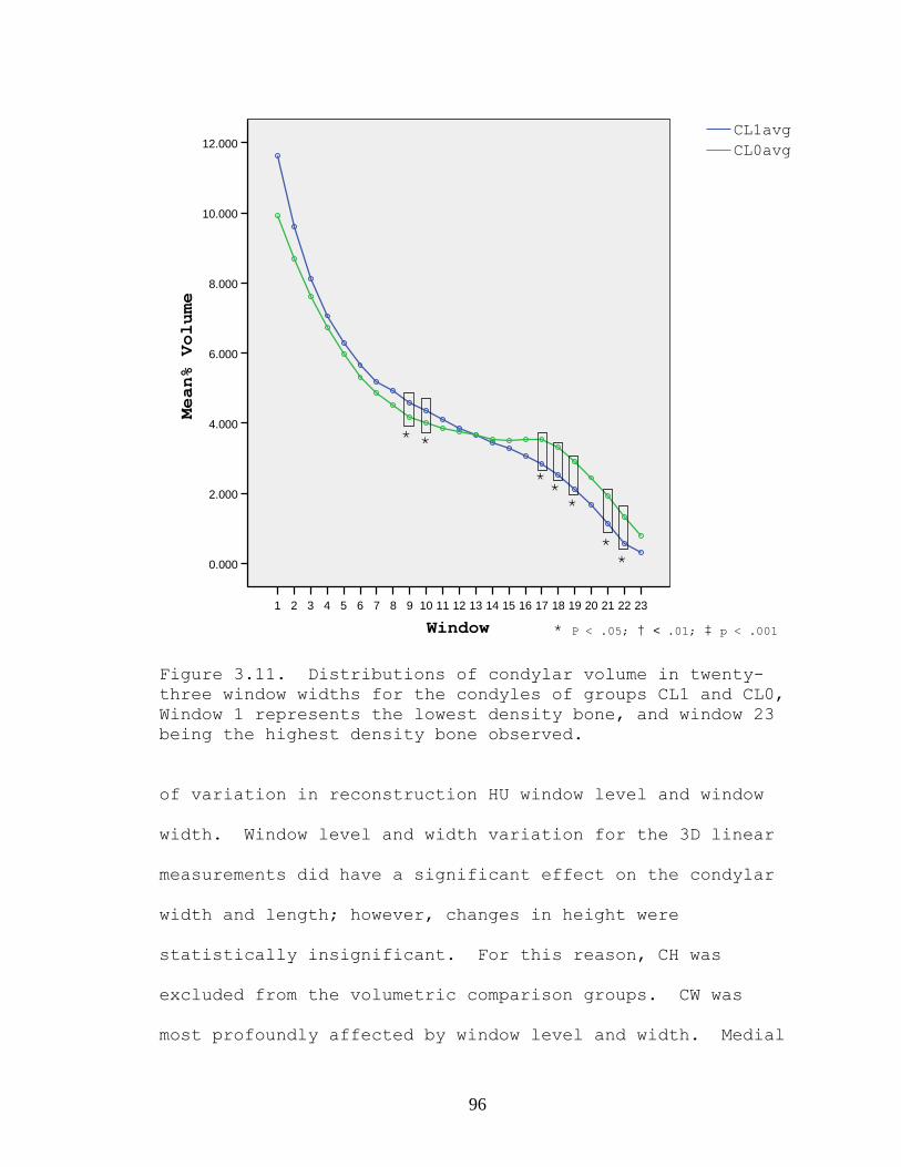
96

2322212019181716151413121110987654321

Window

12.000

10.000

8.000

6.000

4.000

2.000

0.000

Mean% Volume

CL0avgCL1avg

* *

***

**

* P < .05; † < .01; ‡ p < .001

Figure 3.11. Distributions of condylar volume in twenty-three window widths for the condyles of groups CL1 and CL0, Window 1 represents the lowest density bone, and window 23 being the highest density bone observed.

of variation in reconstruction HU window level and window

width. Window level and width variation for the 3D linear

measurements did have a significant effect on the condylar

width and length; however, changes in height were

statistically insignificant. For this reason, CH was

excluded from the volumetric comparison groups. CW was

most profoundly affected by window level and width. Medial

97

2322212019181716151413121110987654321

Window

12.500

10.000

7.500

5.000

2.500

0.000

Mean % Volume

CW0avgCW1avg

* P < .05; † < .01; ‡ p < .001

†

*

†

†

******

*‡‡‡‡†

Figure 3.12. Distributions of condylar volume in twenty-three window widths for the condyles of groups CW1 and CW0, Window 1 represents the lowest density bone, and window 23 being the highest density bone observed. and lateral poles of the 3D condylar reconstructions were

often the first to exhibit areas of erosion, and thereby

producing reduced CW measurements. Significance was found

in the following ranges: -24 to 2476 HU, 76 to 2476 HU, and

176 to 2476 HU. The highest density window level, 176 to

2476 HU, is the recommended window width for viewing bone

98

with V-works™4.0. CL proved to be a challenging dimension

to measure. ICC reliability testing showed measurement

reproducibility to be acceptable; however, the extent of

erosions was difficult to measure with point to point, and

or point to plane measurements. This likely resulted in

fewer windows with significant measurement differences. So

the CL was possibly more profoundly affected by changes in

window level and width than what the results present.

The Hounsfield Unit has been used to describe

physical density and achieve reasonable volume estimates of

anatomic structures.13-15,18,22,23 The greater a tissue

density, the higher the HU numbers will be within the

respective window width. A number of studies have been

performed in efforts to quantify bone density based on

Hounsfield values.13-15 Many of these studies were

accomplished in order to help classify bone types best

suitable to support dental implants.13,14,17 For the present

study, HU window widths and levels are manipulated in order

to create 3D reconstructions most representative of the

anatomic truth. For CW and CL the most accurate windows

were below the recommended window for bone, and extended

into the soft tissue range as defined in Table 3.8. In a

dry skull, extending into the soft tissue range will

enhance visualization. However, in vivo the soft tissue

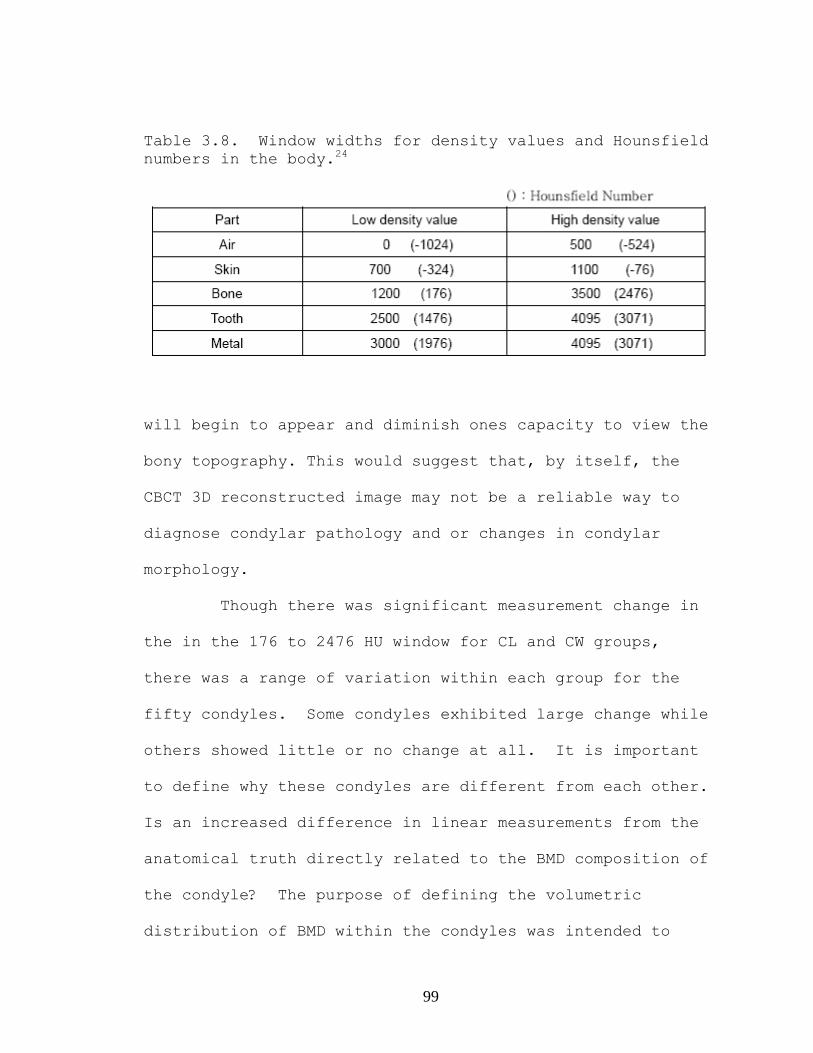
99

Table 3.8. Window widths for density values and Hounsfield numbers in the body.24

will begin to appear and diminish ones capacity to view the

bony topography. This would suggest that, by itself, the

CBCT 3D reconstructed image may not be a reliable way to

diagnose condylar pathology and or changes in condylar

morphology.

Though there was significant measurement change in

the in the 176 to 2476 HU window for CL and CW groups,

there was a range of variation within each group for the

fifty condyles. Some condyles exhibited large change while

others showed little or no change at all. It is important

to define why these condyles are different from each other.

Is an increased difference in linear measurements from the

anatomical truth directly related to the BMD composition of

the condyle? The purpose of defining the volumetric

distribution of BMD within the condyles was intended to

100

answer this very question. The two groups compared

graphically in Figures 3.11 and 3.12 show the volumetric

distribution over 23 density ranges. Significant

differences in bone density distribution were found for

both the CL and CW groups. Windows of significant

difference were in the high and low density ranges. No

significant differences were found in the midrange windows

(WW 10 to WW 14). The number of significant windows was

greater for the CW0/CW1 group than the CL0/CL1 group. One

would expect the CW and CL density distributions to be

alike. They do follow the same pattern; however, the CL

demonstrated fewer windows of significance between the CL0

and CL1 groups. This could relate to the difficulty

presented in measuring morphologic defects in this

dimension. Incapacity to accurately record the anatomic

changes occurring across the range of HU windows could

produce error in condyle selection for the CL0 and CL1

groups; thereby, producing a volumetric comparison between

two groups of condyles with very little variation between

them.

It was not the goal of this study to define the

range of bone mineral densities that constitute the

condyle. A study of this nature would require a sample of

untreated cadaver condyles. Even then, research has shown

101

that, HU are only reliable as BMD predictors in full

trabecular bone, or in the presence of minimal cortical

bone. HU readings from CT scans with thicker cortical bone

become less reliable.15,16 Also, CT numbers can not be

accepted as an absolute for characterization of a tissue

type or lesion.25 CT numbers may vary significantly from

one scanner to another, or even between two scanners of the

same make and model.25,26 However, with some degree of

success, standardized calibration methods have been

employed in efforts to minimize inter-scan discrepancies.27

With attention to detail, strict standardization in all

parameters, continual manufacturer support, and application

of proper calibration methods, reproducibility can be

optimized.28 Studies focused on CT numbers as an accurate

representation of tissue density have, for the most part,

been confined to conventional CT scanners. Recently,

Aranyarachkul et al.13 examined variations in bone density

in designated implant recipient sites using both CBCT and

conventional CT. They found both modalities to be

consistent in their measurements of bone density value;

however, the values were generally higher for CBCT.

Whether CBCT or conventional CT values are closer to

corresponding histological bone densities has yet to be

investigated.

102

Further research on the application of CBCT imaging

in the examination of the TMJ is warranted. One such study

would be to investigate the accuracy and reliability of

CBCT in producing density values that correspond with

histological bone densities. Defining the range and

distribution of expected bone densities within the condyle

may assist the clinician in diagnosis morphologic changes

and pathologic processes within the TMJ. On the medical

side, CT values have already been applied, with some degree

of success, in the differentiation of adrenal masses.29

Nwariaku et al.29 found that a threshold attenuation value

of ≤ 10 HU accurately characterized adrenal cortical

adenomas. This concept could also be applied to the

maxillofacial complex in the evaluation of both hard and

soft tissues.

Conclusions

Due to the relatively high composition of low

density bone within the mandibular condyle, radiographic

assessment, using the 3D reconstruction, is most accurate

when accomplished at density levels below that recommended

for osseous examination. However, utilization of lower

window levels, extending into the soft tissue range, may

compromise ones capacity to view bony topography.

103

Depending on the distribution of bone density within the

condyle, CBCT 3D reconstructed images, by themselves, may

not be a reliable means for diagnosis of condylar pathology

and or changes in condylar morphology. One might, instead,

employ the 3D reconstruction simply as a screening tool,

and perform comprehensive condylar examinations using

progressive crossectional imaging. Using the multiplanar

reconstruction viewing mode is an excellent way to

accomplish this.

104

Acknowledgements

In acknowledgement of the people who have helped on

this thesis project. I would like to thank Dr. Ki Beom Kim

for his constant support and dedication through the entire

process. I would also like to thank Drs. Donald Oliver and

Gus Sotiropoulos for devoting their time, knowledge, and

encouragement along the way. Also, this project would not

have been possible without the help of Dr. Cyrus Alizadeh,

Dr. Becky Schreiner and the Alizadeh Orthodontics staff.

Thank you for your gracious hospitality and selfless

contribution to help make this project a success. Finally,

thanks to Drs. Heidi Israel and Binh Tran for their help

with the statistical analysis of the data.

105

Literature Cited

1. Brooks SL, Brand JW, Gibbs SJ, Hollender L, Lurie AG, Omnell KA et al. Imaging of the temporomandibular joint: a position paper of the American Academy of Oral and Maxillofacial Radiology. Oral Surg Oral Med Oral Pathol Oral Radiol Endod 1997;83:609-618.

2. Quintero JC, Trosien A, Hatcher D, Kapila S. Craniofacial imaging in orthodontics: historical perspective, current status, and future developments. Angle Orthod 1999;69:491-506.

3. Sukovic P. Cone beam computed tomography in craniofacial imaging. Orthod Craniofac Res 2003;6 Suppl 1:31-36; discussion 179-182.

4. Hilgers ML, Scarfe WC, Scheetz JP, Farman AG. Accuracy of linear temporomandibular joint measurements with cone beam computed tomography and digital cephalometric radiography. Am J Orthod Dentofacial Orthop 2005;128:803-811.

5. Mah JK, Danforth RA, Bumann A, Hatcher D. Radiation absorbed in maxillofacial imaging with a new dental computed tomography device. Oral Surg Oral Med Oral Pathol Oral Radiol Endod 2003;96:508-513.

6. Honda K, Larheim TA, Maruhashi K, Matsumoto K, Iwai K. Osseous abnormalities of the mandibular condyle: diagnostic reliability of cone beam computed tomography compared with helical computed tomography based on an autopsy material. Dentomaxillofac Radiol 2006;35:152-157.

7. Kau CH, Richmond S, Palomo JM, Hans MG. Three-dimensional cone beam computerized tomography in orthodontics. J Orthod 2005;32:282-293.

8. Hatcher DC, Aboudara CL. Diagnosis goes digital. Am J Orthod Dentofacial Orthop 2004;125:512-515.

106

9. Ludlow JB, Davies-Ludlow LE, Brooks SL, Howerton WB. Dosimetry of 3 CBCT devices for oral and maxillofacial radiology: CB Mercuray, NewTom 3G and i-CAT. Dentomaxillofac Radiol 2006;35:219-226.

10. Walker L, Enciso R, Mah J. Three-dimensional localization of maxillary canines with cone-beam computed tomography. Am J Orthod Dentofacial Orthop 2005;128:418-423.

11. Lascala CA, Panella J, Marques MM. Analysis of the accuracy of linear measurements obtained by cone beam computed tomography (CBCT-NewTom). Dentomaxillofac Radiol 2004;33:291-294.

12. Marmulla R, Wortche R, Muhling J, Hassfeld S. Geometric accuracy of the NewTom 9000 Cone Beam CT. Dentomaxillofac Radiol 2005;34:28-31.

13. Aranyarachkul P, Caruso J, Gantes B, Schulz E, Riggs M, Dus I et al. Bone density assessments of dental implant sites: 2. Quantitative cone-beam computerized tomography. Int J Oral Maxillofac Implants 2005;20:416-424.

14. Shapurian T, Damoulis PD, Reiser GM, Griffin TJ, Rand WM. Quantitative evaluation of bone density using the Hounsfield index. Int J Oral Maxillofac Implants 2006;21:290-297.

15. Stoppie N, Pattijn V, Van Cleynenbreugel T, Wevers M, Vander Sloten J, Ignace N. Structural and radiological parameters for the characterization of jawbone. Clin Oral Implants Res 2006;17:124-133.

16. Rho JY, Hobatho MC, Ashman RB. Relations of mechanical properties to density and CT numbers in human bone. Med Eng Phys 1995;17:347-355.

17. Hatcher DC, Dial C, Mayorga C. Cone beam CT for pre-surgical assessment of implant sites. J Calif Dent Assoc 2003;31:825-833.

107

18. Mull RT. Mass estimates by computed tomography: physical density from CT numbers. AJR Am J Roentgenol 1984;143:1101-1104.

19. Hounsfield GN. Nobel Award address. Computed medical imaging. Med Phys 1980;7:283-290.

20. Kobayashi K, Shimoda S, Nakagawa Y, Yamamoto A. Accuracy in measurement of distance using limited cone-beam computerized tomography. Int J Oral Maxillofac Implants 2004;19:228-231.

21. Misch KA, Yi ES, Sarment DP. Accuracy of cone beam computed tomography for periodontal defect measurements. J Periodontol 2006;77:1261-1266.

22. Breiman RS, Beck JW, Korobkin M, Glenny R, Akwari OE, Heaston DK et al. Volume determinations using computed tomography. AJR Am J Roentgenol 1982;138:329-333.

23. Kobayashi F, Ito J, Hayashi T, Maeda T. A study of volumetric visualization and quantitative evaluation of bone trabeculae in helical CT. Dentomaxillofac Radiol 2003;32:181-185.

24. Cybermed. V-works™4.0. Seoul, Korea: Cybermed, co, Ltd; 2006: p. Imaging software for real time 3D visualization.

25. Levi C, Gray JE, McCullough EC, Hattery RR. The unreliability of CT numbers as absolute values. AJR Am J Roentgenol 1982;139:443-447.

26. Stadler A, Schima W, Prager G, Homolka P, Heinz G, Saini S et al. CT density measurements for characterization of adrenal tumors ex vivo: variability among three CT scanners. AJR Am J Roentgenol 2004;182:671-675.

27. Cann CE. Quantitative CT for determination of bone mineral density: a review. Radiology 1988;166:509-522.

108

28. Cann CE. Quantitative CT applications: comparison of current scanners. Radiology 1987;162:257-261.

29. Nwariaku FE, Champine J, Kim LT, Burkey S, O'Keefe G, Snyder WH, 3rd. Radiologic characterization of adrenal masses: the role of computed tomography--derived attenuation values. Surgery 2001;130:1068-1071.

109

Vita Auctoris

Brian Albert Schlueter was born on July 12, 1974 to

Robert R. and Marsha A. Schlueter at Wiesbaden Air Force

Base in Wiesbaden, Germany. Shortly after, the Schlueter

family moved back to the states, and Brian and his two

siblings Scott and Amanda were raised in St. Louis,

Missouri.

He attended high school at Westminster Christian

Academy from 1989-1993. Following graduation, Brian

attended Texas Christian University in Fort Worth, TX where

he studied biology and chemistry.

Upon graduation from TCU, Brian was married to

Hollie Marie Anderson; and began his education in dentistry

at SIUE School of Dental Medicine in Alton, IL. After

graduating from SIUE and receiving his degree (DMD), they

moved to Travis Air Force Base, CA where Brian began his

active duty service in the USAF, and attended an advanced

general dentistry residency. While in California, Brian

and Hollie had their first son Noah Grant. Upon completion

of his active duty commitment to the USAF in 2004 at

Whiteman AFB, MO, Brian and his family moved home to St.

Louis, MO to began his orthodontic residency training at

Saint Louis University. On July 19th 2006 they became a

110

family of four with the birth of their second son Parker

Gabriel.

After finishing his orthodontic residency, Brian,

Hollie, Noah and Parker plan to remain in the St. Louis

area, where the rest of their family resides.