configuration and performance of a beowulf

Beowulf clusters in virtually every pricerange are readily available today forpurchase in fully integrated form froma large variety of vendors. At the Uni-

versity of Maryland, Baltimore County (UMBC),my colleagues and I bought a medium-sized 64-processor cluster with high-performance inter-connect and extended disk storage from IBM.The cluster has several critical components, andI demonstrate their roles using a prototype prob-lem from the numerical solution of time-dependent partial differential equations (PDEs).I selected this problem to show how judiciouslycombining a numerical algorithm and its efficientimplementation with the right hardware (in thiscase, the Beowulf cluster) can achieve parallelcomputing’s two fundamental goals: to solveproblems faster and to solve larger problems thanwe can on a serial computer.

System ConfigurationOur cluster—called Kali after the multiarmed In-dian mother goddess—is an IBM 1350 xSeries clus-

ter with 32 dual-processor nodes, a high-performance Myrinet interconnect for parallelcomputations, and a 0.5-Tbyte central disk array(www.ibm.com/servers/eserver/clusters/). We runit with a version of the Linux operating system. Weuse only one possible commodity cluster configu-ration and describe its use in one type of applica-tion area; however, much more powerful systemsshare the same conceptual setup. You can find moreinformation about Kali at www.math.umbc.edu/~gobbert/kali/.

All CPUs are Intel Xeon 2.0-GHz processors.Beowulf clusters became affordable in recent yearsbecause these CPUs are commodity products, mass-produced for the PC market. To obtain the best per-formance from their integration into a parallel com-puter, though, many other vital components must bespecialized and are by no means “commodity” com-ponents (they’re not cheap, either).

One example of vital specialized hardware is theMyrinet interconnect from Myricom (www.myricom.com). Its key features are much-reducedlatency (time delay for a communication to start)compared to conventional Ethernet and a high vol-ume of throughput, rated at 2 Gbits per second(Gbps). Our system includes a 32-port Myrinetswitch composed of four blades with eight portseach. The ports on each blade and the four bladesthemselves are connected via crossbar links.

We use the Myrinet interconnect for communi-

14 COMPUTING IN SCIENCE & ENGINEERING

CONFIGURATION AND PERFORMANCEOF A BEOWULF CLUSTER FOR LARGE-SCALE SCIENTIFIC SIMULATIONS

C L U S T E RC O M P U T I N G

To achieve optimal performance on a Beowulf cluster for large-scale scientific simulations,it’s necessary to combine the right numerical method with its efficient implementation toexploit the cluster’s critical high-performance components. This process is demonstratedusing a simple but prototypical problem of solving a time-dependent partial differentialequation.

MATTHIAS K. GOBBERT

University of Maryland, Baltimore County

1521-9615/05/$20.00 © 2005 IEEE

Copublished by the IEEE CS and the AIP

MARCH/APRIL 2005 15

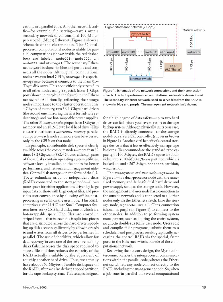
cations in a parallel code. All other network traf-fic—for example, file serving—travels over asecondary network of conventional 100-Mbits-per-second (Mbps) Ethernet. Figure 1 shows aschematic of the cluster nodes. The 32 dual-processor computational nodes available for par-allel computations (shown inside the red dashedbox) are labeled node001, node002, …,node031, and storage1. The secondary Ether-net network is shown in blue and purple and con-nects all the nodes. Although all computationalnodes have two Intel CPUs, storage1 is a specialstorage node because it connects to the main 0.5-Tbyte disk array. This node efficiently serves filesto all other nodes using a special, faster 1-Gbpsport (shown in purple in the figure) in the Ether-net switch. Additionally, reflecting the storagenode’s importance to the cluster operation, it has4 Gbytes of memory, two 36.4-Gbyte hard drives(the second one mirroring the first for fail-safe re-dundancy), and two hot-swappable power supplies.The other 31 compute nodes proper have 1 Gbyte ofmemory and an 18.2-Gbyte local hard drive. Thiscluster constitutes a distributed-memory parallelcomputer—each node’s memory can be accessedonly by the CPUs on that node.

In principle, considerable disk space is clearlyavailable across the compute nodes—more than 32times 18.2 Gbytes, or 582.4 Gbytes, although partsof those disks contain operating system utilities,software locally installed on the nodes for betterperformance, and network and management utili-ties. Central disk storage—in the form of the 0.5-Tbyte redundant array of independent disks(RAID) connected to the storage node—allowsmore space for either applications driven by largeinput data or those with large output files, and pro-vides user convenience by allowing offline post-processing in serial on the user node. This RAIDcomprises eight 73.4-Gbyte Small Computer Sys-tem Interface (SCSI) hard disks, one of which is ahot-swappable spare. The files are stored instriped form—that is, each file is split into piecesthat are distributed across the hard drives, speed-ing up disk access significantly by allowing readsto and writes from all drives to be performed inparallel. The use of checkbits, which allow fordata recovery in case one of the seven remainingdisks fails, increases the disk space required tostore a file and thus reduces the capacity of theRAID actually available by the equivalent ofroughly another hard drive. Thus, we actuallyhave about 367 Gbytes of usable disk space onthe RAID, after we also deduct a spool partitionfor the tape backup system. This setup is designed

for a high degree of data safety—up to two harddrives can fail before you have to resort to the tapebackup system. Although physically in its own case,the RAID is directly connected to the storagenode’s bus via a SCSI controller (shown in brownin Figure 1). Another vital benefit of a central stor-age device is that it lets us effectively manage tapebackups. To accommodate the standard tape ca-pacity of 100 Mbytes, the RAID’s space is subdi-vided into a 100-Mbyte /home partition, which isbacked up, and a 267-Mbyte /scratch partition,which is not.

The management and user node—mgtnode inFigure 1—is a dual-processor node with the same-sized memory and fail-safe dual hard drive andpower supply setup as the storage node. However,the management and user node has a connection tothe outside network and is connected to all othernodes only via the Ethernet switch. Like the stor-age node, mgtnode uses a 1-Gbps connection(shown in purple in Figure 1) to connect to theother nodes. In addition to performing systemmanagement, such as booting the entire system,mgtnode doubles as Kali’s user node. Users editand compile their programs, submit them to ascheduler, and postprocess results graphically, ac-cessing the control RAID via the special, fasterports in the Ethernet switch, outside of the com-putational network.

Reviewing the network design, the Myrinet in-terconnect carries the interprocessor communica-tions within the parallel code, whereas the Ether-net switch lets any node connect directly to theRAID, including the management node. So, whena job runs in parallel on several computational

node001 node031node002 mgtnode

Myrinet switch

Ethernet switch

High-performance network (2 Gbps)

100

Mbp

s

100

Mbp

s

100

Mbp

s

100

Mbp

s

1 G

bps

1 G

bps

(0.5 Tbytes)RAID

Outside network

storage1

Figure 1. Schematic of the network connections and their connectionspeeds. The high-performance computational network is shown in red.The secondary Ethernet network, used to serve files from the RAID, isshown in blue and purple. The management network isn’t shown.


nodes, including, potentially, the storage node, thecode’s internal communications occur via theMyrinet, whereas the code accesses input and out-put files on the RAID via the Ethernet. After com-pleting the job, the user performs the postprocess-ing in serial on the user node, outside thecomputational network. For alternative choicesfor the configuration of the cluster, see the “Al-ternative Setups” sidebar.

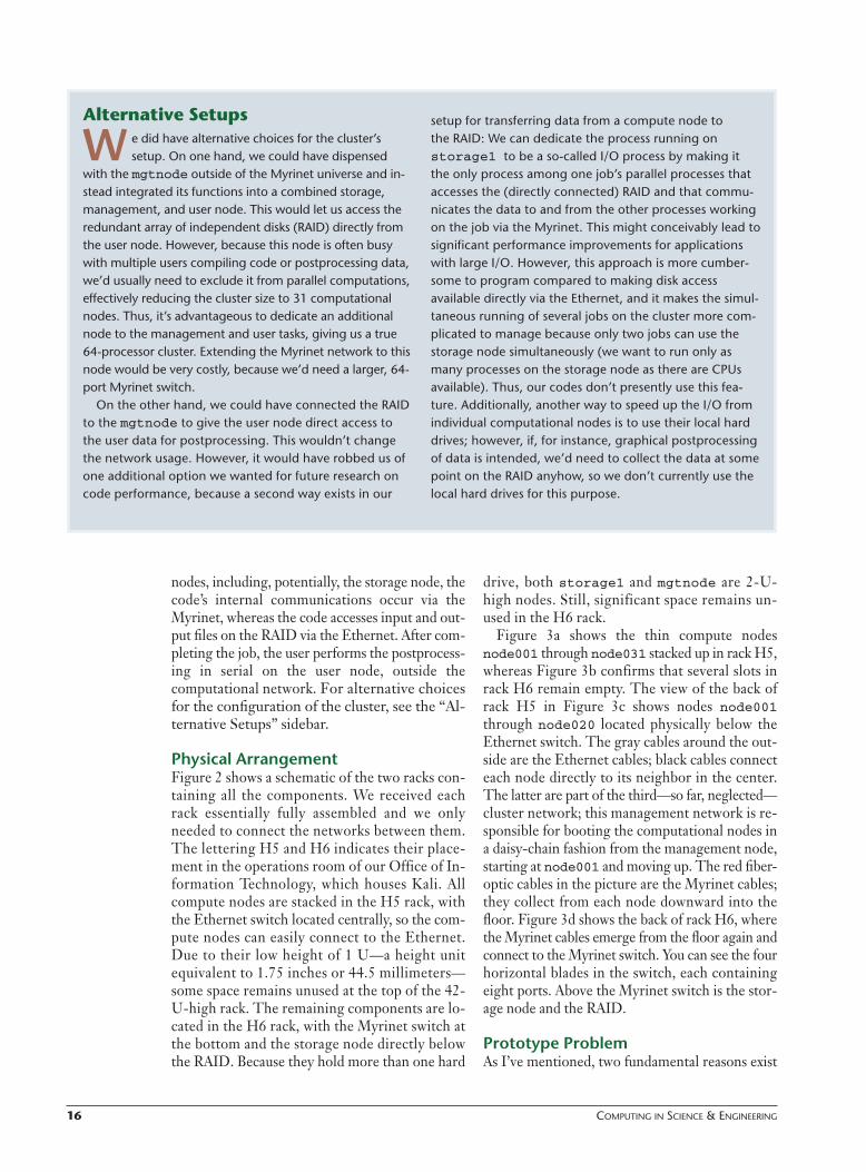
Physical ArrangementFigure 2 shows a schematic of the two racks con-taining all the components. We received eachrack essentially fully assembled and we onlyneeded to connect the networks between them.The lettering H5 and H6 indicates their place-ment in the operations room of our Office of In-formation Technology, which houses Kali. Allcompute nodes are stacked in the H5 rack, withthe Ethernet switch located centrally, so the com-pute nodes can easily connect to the Ethernet.Due to their low height of 1 U—a height unitequivalent to 1.75 inches or 44.5 millimeters—some space remains unused at the top of the 42-U-high rack. The remaining components are lo-cated in the H6 rack, with the Myrinet switch atthe bottom and the storage node directly belowthe RAID. Because they hold more than one hard

drive, both storage1 and mgtnode are 2-U-high nodes. Still, significant space remains un-used in the H6 rack.

Figure 3a shows the thin compute nodesnode001 through node031 stacked up in rack H5,whereas Figure 3b confirms that several slots inrack H6 remain empty. The view of the back ofrack H5 in Figure 3c shows nodes node001through node020 located physically below theEthernet switch. The gray cables around the out-side are the Ethernet cables; black cables connecteach node directly to its neighbor in the center.The latter are part of the third—so far, neglected—cluster network; this management network is re-sponsible for booting the computational nodes ina daisy-chain fashion from the management node,starting at node001 and moving up. The red fiber-optic cables in the picture are the Myrinet cables;they collect from each node downward into thefloor. Figure 3d shows the back of rack H6, wherethe Myrinet cables emerge from the floor again andconnect to the Myrinet switch. You can see the fourhorizontal blades in the switch, each containingeight ports. Above the Myrinet switch is the stor-age node and the RAID.

Prototype ProblemAs I’ve mentioned, two fundamental reasons exist

Alternative Setups

W e did have alternative choices for the cluster’ssetup. On one hand, we could have dispensed

with the mgtnode outside of the Myrinet universe and in-stead integrated its functions into a combined storage,management, and user node. This would let us access theredundant array of independent disks (RAID) directly fromthe user node. However, because this node is often busywith multiple users compiling code or postprocessing data,we’d usually need to exclude it from parallel computations,effectively reducing the cluster size to 31 computationalnodes. Thus, it’s advantageous to dedicate an additionalnode to the management and user tasks, giving us a true64-processor cluster. Extending the Myrinet network to thisnode would be very costly, because we’d need a larger, 64-port Myrinet switch.

On the other hand, we could have connected the RAIDto the mgtnode to give the user node direct access tothe user data for postprocessing. This wouldn’t changethe network usage. However, it would have robbed us ofone additional option we wanted for future research oncode performance, because a second way exists in our

setup for transferring data from a compute node to the RAID: We can dedicate the process running onstorage1 to be a so-called I/O process by making itthe only process among one job’s parallel processes thataccesses the (directly connected) RAID and that commu-nicates the data to and from the other processes workingon the job via the Myrinet. This might conceivably lead tosignificant performance improvements for applicationswith large I/O. However, this approach is more cumber-some to program compared to making disk accessavailable directly via the Ethernet, and it makes the simul-taneous running of several jobs on the cluster more com-plicated to manage because only two jobs can use thestorage node simultaneously (we want to run only asmany processes on the storage node as there are CPUsavailable). Thus, our codes don’t presently use this fea-ture. Additionally, another way to speed up the I/O fromindividual computational nodes is to use their local harddrives; however, if, for instance, graphical postprocessingof data is intended, we’d need to collect the data at somepoint on the RAID anyhow, so we don’t currently use thelocal hard drives for this purpose.

MARCH/APRIL 2005 17

for using parallel computing: First, using severalprocessors in parallel to attack a problem shouldhelp obtain the solution more quickly. Second, andmore fundamentally, distributing a problem ontoseveral processors can help solve a problem that’stoo large for a serial machine. The following pro-totype problem will demonstrate both these ad-vantages. The application concerns the flow of cal-cium ions in a single human heart cell.1,2 Themodel consists of a system of reaction-diffusionequations with nonlinear reaction terms and ahighly nonsmooth source term with a probabilisticcomponent in the calcium equation. The simula-tion domain � represents one heart cell, which wecan acceptably model as a brick � := (–X, X ) � (–Y,Y ) � (–Z, Z ) � �3 with one longer dimension Z >X = Y. Realistic numbers are X = Y = 6.4 and Z =32.0, measured in micrometers.

To focus on parallel computing, let’s consider asimpler prototype problem that neglects the reac-tions between the species and the calcium source butretains the realistic diffusive transport of the calciumions. Whenever choices are required in the follow-ing, we’ll let the application problem guide us. In ef-fect, the study reported here is a thorough test of ourmethod’s core and its implementation.

Find u(x, y, z, t) for all (x, y, z) � � and 0 � t � Tsuch that

in � for 0 < t � T, (1a)

n • (D∇u) � 0 on �� for 0 < t � T, (1b)

u = uini(x, y, z) in � at t = 0, (1c)

where n = n(x, y, z) denotes the unit outward nor-mal vector at surface point (x, y, z) of the domainboundary ��. Here, T denotes the final time forthe simulations, and the diagonal matrix D =diag(Dx, Dy , Dz) consists of the diffusion coeffi-cients in the three coordinate directions. To modelthe diffusion behavior realistically, we pick thesame values as in the application example Dx = Dy= 0.15 and Dz = 0.30 in micrometers squared overmilliseconds. As the initial distribution, we pick thesmooth function

uini(x, y, z) = .

To get an intuitive feel for the solution behavior,observe that the PDE in Equation 1a has no

source term and that we prescribe no-flowboundary conditions on the entire boundary inEquation 1b. Hence, the chemical will diffusethrough the domain without escaping from it,starting from the nonuniform initial distribution(Equation 1c), until the chemical reaches a steadystate, constant throughout the cell. Because thesystem conserves mass, we can analytically com-pute the constant steady-state solution as uSS �1/8 for future reference.

We can obtain the true solution for this linearconstant-coefficient problem on a rectangular do-main analytically, for instance, by separation ofvariables and Fourier analysis. We give this as

(2)

where �x = �/X, �y = �/Y, and �z = �/Z. Now, wecan use this true solution to gauge a priori whatvalue of the final time T is suitable for approachingthe steady-state solution. We reach this steady statewhen all exponential function terms in Equation 2become vanishingly small. Given the realistic val-

u x y z tx D tx x x

y

( , , , )cos( )exp( )

cos(

=+ −

×+

12

1

2λ λ

λ yy D t

z D t

y y

z z z

)exp( )

cos( )exp( ),

−

×+ −

λ

λ λ

2

22

12

cos cos cos2 2 22 2 2π π πxX

yY

zZ

∂∂

− ∇ ⋅ ∇ =ut

D u( ) 0

node001

node002

node003

node031

node030

node020

node021

Rack H6

mgtnode

Screen and keyboard

RAID (0.5 Tbytes)

Ethernet switch

Myrinet switch

storage1

Rack H5

Figure 2. A schematic of the Kali components’physical arrangement in their two racks. H5 holds allthe compute nodes and the Ethernet switch,whereas H6 holds the remaining components,including the Myrinet switch, the storage node, andthe user node.


ues chosen already for the diffusion coefficients andthe domain size, the choice T = 1,000.0 millisec-onds is the smallest suitable value because then thelargest exponential term is exp(–Dz�z

2t) 0.055.Although the application problem doesn’t tend toa steady state, this time scale is still interesting tostudy because it reveals the underlying time scaleassociated with the diffusion in the system withoutsource and reaction times.

Numerical MethodWe’ve demonstrated in previous work that amethod-of-lines approach using finite elements forthe spatial discretization converges for the applica-tion problem,3 and we continue using it here. Gen-

eral background on finite-element methods fortime-dependent PDEs is available.4,5 To use as lit-tle memory as possible, we restrict ourselves tonodal basis functions that are linear in each coor-dinate direction. Because the domain � is itself abrick, it makes sense to discretize it uniformly intosmaller brick elements of volume (x)(y)(z),where x, y, and z denote the mesh spacings inthe three coordinate directions.

One challenge for numerically solving this ap-plication problem with the required accuracy re-sults from the need for an extremely high gridresolution for the domain. Calcium ions enter thecell through calcium channels, modeled on thislength scale as point sources at calcium releaseunits. These CRUs are distributed throughoutthe cell at distances of xCRU = yCRU = 0.8 andzCRU = 2.0, measured in micrometers.2 Thisgives a CRU lattice that’s 16 � 16 � 32 in our celldomain �. Using the rule of thumb that we wishto place at least eight mesh points betweenCRUs, we want to use at least 128 elements in thex and y directions and 256 in the z direction.However, to further guarantee that the meshspacing z := 2Z/Nz is approximately equal to x= y, we increase the resolution in the z directionand consider a mesh with 128 � 128 � 512 ele-ments for the application problem.

To understand this resolution’s complexity, let’scompute the number of degrees of freedom N,finite-element terminology for the number of un-knowns the code must determine. In the method-of-lines approach, we’re referring to the spatial dis-cretization here because we must determine theseunknowns at every time step. Denote by Nx = Ny =129 and Nz = 513 the number of points on whichthe solution is based for a mesh with 128 � 128 �512 elements. This gives N = (Nx)(Ny)(Nz) =8,536,833, or more thn 8.5 million unknowns. Ifthe code stores each unknown as one double-precision number using 8 bytes of memory pernumber, it takes roughly 65 Mbytes to store the so-lution in memory. Table 1 shows these and otherpredictions for four possible mesh resolutions. Wecan see already that for the finest resolution of 256� 256 � 1,024, storing its solution with over 67.7million unknowns requires roughly 517 Mbytes, aformidable number even on a workstation with, say,1 Gbyte of memory.

A method-of-lines discretization of a PDE suchas ours results in a stiff system of ordinary differ-ential equations (ODEs).6 To avoid the severe re-striction on the time step t that would result fromusing an explicit time-stepping method in thiscase, we use the implicit Euler method, which—

(a)

(c)

(b)

(d)

Figure 3. Photographs of the cluster. The (a) compute nodes in rack H5and the (b) remaining components in rack H6 are connected bynetwork cables in (c) the back of rack H5 (lower half pictured) and (d)the back of rack H6 (bottom part pictured). (Photographs courtesy ofRandy Philipp, UMBC Office of Information Technology.)

MARCH/APRIL 2005 19

although only first-order accurate—will requirethe least memory among implicit methods. An im-plicit time-stepping method for our linear PDEinvolves the solution of a linear system of di-mension N in every time step. Using a conven-tional direct solver, such as Gaussian elimina-tion, requires us to store the system matrix ofsize N � N. Even in sparse storage (meaning onlynonzero entries are stored), this would be prohib-itively expensive for our desired N values because27 essentially nonzero diagonals in the system ma-trix exist from the finite-element discretization inthree dimensions.3 We’ve avoided this storage costentirely by switching to an iterative solver for thislinear system—the conjugate-gradient (CG)method is appropriate for this symmetric prob-lem—and by using a matrix-free implementationof the matrix-vector product in the iterativemethod. Thus, our only memory requirements areapproximately 10 auxiliary vectors of dimension Nin addition to the solution at the current time step.(This isn’t necessarily the smallest number of aux-iliary vectors possible, but because the applicationproblem will require a couple of extra vectors, wearen’t yet optimizing the code in this respect.)With the number of all significantly sized variablesestablished, we can compute the predicted mem-ory needed for the entire code on a serial machine(see Table 1). We see immediately that 128 � 128� 512, requiring 716 Mbytes of memory, is thefinest resolution that fits on a machine with 1Gbyte of memory. We can see already that paral-lel computing will yield a benefit if we can com-pute the solution with a finer resolution than pos-sible on a serial machine.

Using the implicit Euler method, the time stept isn’t restricted due to stability, so we can use any(positive) value. We exploit this by implementingautomatic time-stepping, which controls t suchthat the estimator for the local truncation error sat-isfies a chosen tolerance.6 The automatic step-sizecontrol is the key to saving time for simulations oftransient problems with large final times such as T= 1,000.0. We’re also using the study in this article

to test this part of the code’s functionality.

Output ConsiderationsTo look at the solution at numerous time steps, wesolve the transient problem, first saving solutiondata for several chosen time steps to disk, thenpostprocessing the data. To realistically determinehow often to save the solution to disk, consider thatthe application model2 lets the CRUs open andclose with frequency tCRU = 1.0 milliseconds.Thus, we want to save the solution to disk with thesame frequency; for 0 � t � T = 1,000.0, we need tosave 1,001 frames. Currently, we use output inASCII format at present for best compatibility withall versions of our postprocessing software, Matlab(www.mathworks.com). To accurately capture thedouble-precision variables, we use 26 bytes for eachnumber. The final column of Table 1 shows howmuch estimated disk space is required to save thismany frames. For a parabolic problem such asEquation 1, known to have a very smooth solution,we could save significant disk space by outputtingthe solution at, say, every other point. In the appli-cation problem however, the probabilistic compo-nent in the nonsmooth source term can create con-centration increases in any part of the domain atany time, so we need to be prepared to save the en-tire solution for postprocessing.

For the resolution 128 � 128 � 512, for exam-ple, we need roughly 207 Gbytes of disk space tosave the results of one complete simulation. Al-though possible in principle in the /scratch par-tition of our RAID, it could cause problems inpractice if other users already have data stored.But for the finest resolution 256 � 256 � 1,024, wewould need 1,641 Gbytes to save all 1,001 framesof the solution simultaneously to disk; this muchdisk space isn’t available. To work around this, weneed to postprocess the solution at every time stepon the fly, meaning that the solution is post-processed in all desired ways immediately after it’scomputed, and then it’s deleted. This also impliesthat using ASCII storage isn’t a seriously limitingfactor at present because switching to binary stor-

Resolution Degrees of Predicted memory Predicted memory Predicted disk freedom N need for solution need for serial space for 1,001

(Mbytes) code (Mbytes) frames (Gbytes)32 � 32 � 128 140,481 1 12 364 � 64 � 256 1,085,825 8 91 26128 � 128 � 512 8,536,833 65 716 207256 � 256 � 1,024 67,700,225 517 5,682 1,641

Table 1. Predicted memory and disk space usage (results are rounded).


age using 8 bytes per double-precision numberwould decrease the disk space requirement by afactor of only 3.25. Although significant, the sav-ings associated with postprocessing on the fly aremuch greater. This shows that output considera-tions are an issue for the solution of time-dependent PDEs, and having significant centraldisk space is necessary to facilitate the convenientpostprocessing of combined data from all proces-sors on the user node.

Parallel ImplementationOn a distributed-memory cluster, the choice ofdata structure is crucial because it can make thedifference between a method that scales well tomany parallel processes and one that doesn’t. Weopted for the simplest one-dimensional decom-position of the data to get the cleanest code pos-sible with clear communication patterns. Thedomain � is divided into P nonoverlapping sub-domains, one on each of the P parallel processes,numbered 0 � p < P. We divide � in the long, orz, direction. This means that each process con-tains approximately Nz/P x-y planes of (Nx)(Ny)points. Using a column-oriented data structure—such as the one Matlab uses—makes each x-yplane’s nodal values contiguous. This and theresulting simplicity of Matlab’s postprocessing in-terface drove our choice, at the expense of nu-merical efficiency, which might improve by, say, ared-black ordering of the points. To fully controlthe memory usage, we program in C, using theIntel compiler icc. We use the message-passinginterface MPI,7 currently the most popular libraryfor parallel communications, because of its porta-bility; specifically, we use the Myricom imple-mentation of MPI based on MPI’s popularMPICH implementation.7

The most significant amount of communicationis required inside the iterative solver as part of thematrix-free matrix-vector product, where allprocesses 1 � p < P – 1 must receive the values onthe last x-y plane of process p – 1 and on the first x-y plane of process p + 1 at every iteration; processesp = 0 and p = P – 1 each require only one of these.Correspondingly, processes 1 � p < P – 1 need tosend their first x-y plane to process p – 1 and theirlast x-y plane to process p + 1. These communica-tions between neighboring processes are imple-mented by nonblocking MPI_Isend/MPI_Irecvcommands,8,9 meaning that during the communi-cation phase, the processes can simultaneously per-form other calculations that don’t depend on anyof the values being received. The only other typeof communication that occurs in the iterative

method is that of scalar products between vectors.Because the results of the scalar products areneeded on all processes, MPI_Allreduce com-mands are used.8,9 Every iteration of the iterativesolver has exactly two such communications, andour memory-optimal implementation of the CGmethod has been shown to scale very well for atleast 32 processes.10

Aside from calling the iterative solver at everytime step, the (not yet fully optimized) ODEmethod itself uses three matrix-vectormultiplications per time step as well as a fewMPI_Allreduce communications per timestep—one each for the solution’s norm and the es-timator of the local truncation error and additionalones for computing diagnostic output such asmin(u) and max(u), which we choose to calculateat every time step. There are an order of magni-tude fewer ODE steps than CG iterations, whichis why communications in the iterative solver arethe most costly.

One adage of successful parallel programmingregarding communication is “don’t.” That is, it’sbest to design algorithms that communicate asrarely as possible. In MPI, the programmer explic-itly requests all communications using calls to MPIfunctions. Thus, one of MPI’s best features is thatit keeps the programmer aware of all communica-tions, which often leads to a reflection on thechoice of algorithm or to improvements in thecode’s communication structure.

Simulation Results and Numerical PerformanceWe can solve Equation 1 on meshes with the fourresolutions that Table 1 lists. Figure 4 shows sliceplots of the solution for the resolution 32 � 32 �128 at different times; the domain’s long dimensionis oriented from left to right in the plots. Besidesslices at the bottom and the back of the domain,which act as visual guides to the domain shape, weselect slices at x = 0, y = 0, and z = 0 through thecenter of the domain and two additional ones at z= –16 and z = +16 in the long dimension. The firstplot shows the initial solution’s symmetry and cov-ers the full color range from dark blue for u = 0 onthe domain boundary to red for u = 1 in the center.Throughout the subsequent plots, the solution dif-fuses rapidly through the domain. By t = 100, thesolution starts approaching its steady-state value ofuSS � 1/8—visible in light blue in the central partof the domain up to and including the boundariesin x and y on the slice z = 0. We can see this processcontinue by t = 200 and note that the solution atthe boundaries of z = ± Z also starts reaching the

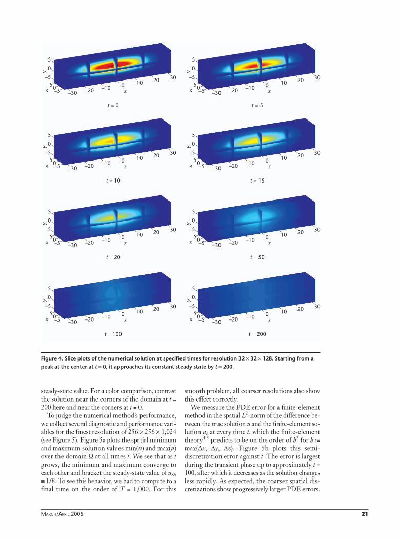
MARCH/APRIL 2005 21

steady-state value. For a color comparison, contrastthe solution near the corners of the domain at t =200 here and near the corners at t = 0.

To judge the numerical method’s performance,we collect several diagnostic and performance vari-ables for the finest resolution of 256 � 256 � 1,024(see Figure 5). Figure 5a plots the spatial minimumand maximum solution values min(u) and max(u)over the domain � at all times t. We see that as tgrows, the minimum and maximum converge toeach other and bracket the steady-state value of uSS� 1/8. To see this behavior, we had to compute to afinal time on the order of T = 1,000. For this

smooth problem, all coarser resolutions also showthis effect correctly.

We measure the PDE error for a finite-elementmethod in the spatial L2-norm of the difference be-tween the true solution u and the finite-element so-lution uh at every time t, which the finite-elementtheory4,5 predicts to be on the order of h2 for h :=max{x, y, z}. Figure 5b plots this semi-discretization error against t. The error is largestduring the transient phase up to approximately t =100, after which it decreases as the solution changesless rapidly. As expected, the coarser spatial dis-cretizations show progressively larger PDE errors.

x

5

0

–550–5 –30 –20 –10 0 10 20 30

t = 0

z

y

x

5

0

–550–5 –30 –20 –10 0 10 20 30

t = 10

z

y

x

5

0

–550–5 –30 –20 –10 0 10 20 30

t = 20

z

y

x

5

0

–550–5 –30 –20 –10 0 10 20 30

t = 5

z

y

x

5

0

–550–5 –30 –20 –10 0 10 20 30

t = 15

z

y

x

5

0

–550–5 –30 –20 –10 0 10 20 30

t = 50

z

y

x

5

0

–550–5 –30 –20 –10 0 10 20 30

t = 100

z

y

x

5

0

–550–5 –30 –20 –10 0 10 20 30

t = 200

z

y

Figure 4. Slice plots of the numerical solution at specified times for resolution 32 � 32 � 128. Starting from apeak at the center at t = 0, it approaches its constant steady state by t = 200.


Figure 5c plots the local time step t used tocompute the numerical solution at every time t; re-call that the code uses variable time-stepping withautomatic control of the estimated local truncationerror, hence t isn’t constant. We used a toleranceof 10–6 for this ODE error. The time step startsout as t = 0.03125, after which it doubles pro-gressively to the maximum permitted value of t =0.5. Using automatic step-size control gives us amajor gain in efficiency without a loss of accuracy.This is why we use an implicit method for thisproblem, despite the more complicated codingcompared to an explicit method; t is not re-stricted in magnitude, and the automatic step-sizecontrol can pick a large value for it. A total of3,085 time steps are taken, over one-third of thoseincurred by t = 100. Somewhat surprisingly, thenumber of time steps is practically the same whenusing the coarser resolutions.

Recall that at every time step, we use the CGmethod to solve a linear system of equations. Weuse a tolerance of 10–3; tighter tolerances didn’timprove the PDE error in Figure 5b appreciably.Figure 5d reports the number of iterations thismethod took at every time t. It uses fewer itera-tions initially when the time step t is small andmore around t = 100, where the solution is stillchanging somewhat but t has already increased.Then, the iteration numbers settle down toroughly 14 for the remaining time steps. Nearlyhalf of the total 41,817 iterations are incurred by t= 100; for the coarser resolutions, fewer CG iter-ations are needed at each time step. The numberof CG iterations remains reasonably small, evenfor the finest resolution 256 � 256 � 1,024, whichjustifies using an unpreconditioned iterativemethod. This is good because it’s difficult to devisea preconditioner that doesn’t require additional

0 200 400 600 800 1,0000.000

0.125

0.250

0.375

0.500

0.625

0.750

0.875

1.000

0 200 400 600 800 1,0000

0.5

1.0

1.5

2.0

2.5

3.0

3.5

4 0

4.5×10–3

(a) (b)

0 200 400 600 800 1,0000.0000

0.0625

0.1250

0.1875

0.2500

0.3125

0.3750

0.4375

0.5000

3,085 steps

0 200 400 600 800 1,0000

5

10

15

20

25

30

35

41,817 steps

(c) (d)

Figure 5. The diagnostic and performance output plotted versus time t for the finest resolution 256 � 256 �1,024. They demonstrate that the code computes the solution accurately and that the numerical method isefficient: (a) minimum and maximum of the solution u over domain �; (b) L2-norm of the true error u – uh; (c)variable time step t used; and (d) number of conjugate-gradient (CG) iterations required.

MARCH/APRIL 2005 23

communications (which would make the precon-ditioning as costly as additional CG iterationsthemselves) and that can be implemented in ma-trix-free form (because we can’t afford any addi-tional storage).

Parallel PerformanceBefore discussing Kali’s performance, I must firstpresent some details regarding the parallel runs.We ran our code for the four different resolutionslisted in Table 1 and with P = 1, 2, 4, 8, 16, and 32parallel processes. The code run with 1 process isactually the parallel code run on 1 process, but, be-cause all communication commands are condi-tional on P > 1, this code is equivalent to a serialcode of the same algorithm. In all cases, a run withP processes uses only one CPU on each of P nodesused. Thus, each process has each node’s entire 1Gbyte of memory available.

Memory PerformanceIn Table 1, we analytically predicted the memoryrequired for serial code. Using the Unix com-mand top, we observe now how much memorythe code actually uses per process. We understandthat this might not be the most accurate way tomake these observations, but, if they confirm ouranalytic predictions, we feel confident about theirvalidity, whereas a significant disagreement canpoint to bugs (for example, memory leaks, if theobserved memory usage keeps increasing overtime). Table 2 collects these observations for allstudies performed. For P = 1, we see that the ob-served values in Table 2 are just slightly higherthan the analytic predictions in Table 1. Thisconfirms that our predictions are reasonable andthat the code doesn’t use any surprising addi-tional memory. Jumping from the 1-process casesto the cases of the finest resolution 256 � 256 �1,024, we notice, as expected, that the finest res-olution can’t run on one node. In fact, we need touse at least P = 8 nodes to accommodate theproblem. Recall that only one parallel processruns on each dual-processor node—otherwise,this amount of memory per process couldn’t evenbe accommodated for P = 8 because both CPUs

on a node share the same 1 Gbyte of memory.The value of 731 Mbytes itself appears so far toagree with the predicted memory requirement of5,682 Mbytes divided by P = 8. Comparing thememory usage per process from one P value tothe next for the resolution 256 � 256 � 1,024, wenotice that memory per process is not halved ex-actly, which requires an explanation.

Also surprising is the observed memory usage forthe resolution 32 � 32 � 128 for more than oneprocess—because the solution and all auxiliary vec-tors are now split across two processes, we’d expectthe code to use less memory per process, but weobserve the opposite. I believe the explanation isthat the MPI libraries are actually only loaded atruntime for P > 1 and that they take up a majorchunk of memory for such a coarse resolution.Looking at the P = 2 case, we hypothesize that thischunk should be 28 Mbytes minus half of the pre-dicted serial memory of 12 Mbytes—that is, 22Mbytes. I can now in turn try to predict the mem-ory per process required for the P = 2 run of theresolution 64 � 64 � 256. To the baseline 22Mbytes, add half of the predicted serial memory of91 Mbytes from Table 1 to get a prediction of 67Mbytes, which is close to the observed 70 Mbytes.This formula—a baseline of 22 Mbytes plus thepredicted serial memory from Table 1 divided byP—allows surprisingly accurate predictions for allother resolutions and cases of P. It also explains thebehavior observed in Table 2 for the finest resolu-tion 256 � 256 � 1,024.

Although appearing rather pedantic, this exer-cise demonstrates that we can make sense of thememory usage that the operating system commandtop reports. It also shows the benefit of finding away to compare predicted and observed memoryusage carefully as a tool to debug and to optimizememory usage in a parallel code.

Speed PerformanceFinally, after we’ve confirmed that the solution iscorrect (we wouldn’t want a code that gives in-correct results, no matter how fast it is), that thenumerical method behaves as desired (we don’twant a bad numerical method), and that we can

Table 2. Observed memory usage per process (in Mbytes).

Resolution P = 1 P = 2 P = 4 P = 8 P = 16 P = 32 32 � 32 � 128 14 28 28 28 28 22 64 � 64 � 256 97 70 46 34 28 26128 � 128 � 512 721 379 200 111 68 45256 � 256 � 1,024 n/a n/a n/a 731 377 202


indeed solve problems of significant size, we’reready to enjoy the final benefit of parallel perfor-mance: the speedup. We time the method by ob-taining the wall-clock time from MPI_Wtimebefore the start and after the end of the ODEmethod and computing their difference. Wemust use a measure such as wall-clock time forparallel code—as opposed to CPU time, for ex-ample—because communications are inherent toparallel computing and thus must be taken intoaccount. Recall that the idea of parallel comput-ing was to distribute the calculation work into Pparallel processes and to obtain the result P timesas fast. However, although dividing the calcula-tions into P processes means that the calculationcost gets better as P increases, a truly parallel coderequires communications among those Pprocesses, whose cost gets worse as P increases.This increasing communication cost in the face ofdecreasing calculation cost per process quickly be-comes a challenge, an effect compounded by thefact that calculations on today’s workstations areseveral orders of magnitude faster than commu-nications. Because of these issues, the only honestway to measure timing for a parallel code is to in-clude both calculations and communications,which we can do by recording wall-clock time, forinstance. This is a tough but realistic measure ofperformance because it also includes various un-avoidable operating system and network slow-downs associated with real-life system operation(for an alternative measure of speedup, see the“Scaled Speedup” sidebar).

Table 3 reports the wall-clock times observed forthe code in hours:minutes:seconds. Comparing theresults for the P = 1 times for the different resolu-tions shows how rapidly the problem’s complexity

and resulting times increase when refining the nu-merical mesh. By using more processes, however,we can reduce the times dramatically. To put thetimes for the finest resolution in perspective, wecan solve a problem with no fewer than 67.7 mil-lion degrees of freedom from t = 0 to T = 1,000.0in less than an overnight run when using 32 nodes.

The times in Table 3 are approximately halved innearly all cases when we double the number of par-allel processes. This property begins to break downfor the largest number of processes, P = 32. We canvisualize the effect of decreasing times with increas-ing P by plotting observed speedup SP against P. Here,we define SP := T1/TP for a fixed problem size as thefraction of observed time T1 on 1 process over ob-served time TP on P processes. In the optimal case,in which TP = T1/P, the speedup will then be SP = P.

Figure 6a shows the observed speedup for all fourresolutions used. The dashed line is the optimalspeedup SP = P. By definition, speedup plots startat the value SP = 1 for P = 1. As the communica-tion time increases relative to the calculation time,the speedup curves eventually fall below the opti-mal value. To get the comparable visual effect forthe finest resolution 256 � 256 � 1,024, we mod-ify its definition of speedup to SP := 8T8/TP; thus,it starts at the optimal value for P = 8, the small-est P available. The four lines are remarkablyclose to the optimal value. At P = 16, we have SP 15 for all resolutions, which is still very close tothe optimal value of 16. By P = 32, the differentresolutions start showing a range of values fromSP 28 for the coarsest to SP 31 for the finestresolution. Typically, speedup is better the largerthe problem’s complexity. This phenomenon re-sults from the fact that, in this case, the calcula-tion time remains a larger percentage of the com-

Scaled Speedup

O ur computational experiments solve problems offixed size to observe speedup of the parallel code.

An alternative is the observed scaled speedup, a concept inwhich the problem size increases (for example, doubles)with each increase (doubling) of the number of processesP. This measure keeps the calculation time and memoryusage per process as high as possible on each process,which blunts the effect of the communication cost in-creasing with increasing P. This measure, therefore, nicelycombines a demonstration of solving larger problemsfaster with increasing P. For our algorithm, though, thisconcept is difficult to apply. We could keep the memory

usage per process constant as P is doubled by doublingNz, which would have resulted in the degrees of freedomN doubling for fixed Nx and Ny. However, the complexityof a transient run of our algorithm also involves the num-ber of conjugate-gradient (CG) iterations, which wouldhave increased with N. Thus, the algorithm’s complexityper process more than doubles with doubling P, which isinconsistent with the definition of scaled speedup. Thus,we restricted ourselves to the conventional definition ofspeedup; in this sense, our speedup is a tougher measureof performance because the decreasing calculation com-plexity per process works against us as P increases alongwith the increasing communication cost.

MARCH/APRIL 2005 25

bined calculation and communication time. Oneway to gauge the complexity per process of aCPU-intensive job is to look at the memory usageper process. As Table 2 indicates, the memory us-age per process falls quite dramatically for thelarger P values, letting us conclude that not muchcalculation work is left to do per process, at leastfor the coarser resolutions.

Figure 6b shows another quantity whose valuecan characterize the scalability of parallel code. Theobserved efficiency EP is the ratio of speedup SP overP. Hence, a value of EP = 1 or 100 percent is opti-mal. The efficiency plot is often useful in bringingout certain features that are easily overlooked in thespeedup plot. For instance, we see in Figure 6b thatefficiency drops off by P = 4 for several cases, morerapidly than is visible in the speedup plot. But itdoesn’t drop off any further for larger values of Pand is still roughly 95 percent for most resolutionsat P = 16. At P = 32, we see again a range of valuesfor the different resolutions, from approximately87 percent for the coarsest to about 97 percent forthe finest resolution. These speedup and efficiencyresults are excellent for a tightly coupled algorithmon a distributed-memory cluster such as this one,and illustrates the power of Kali’s high-performance interconnect.

You might think at this point that we chose touse only one CPU per node in the parallel studyfor memory reasons alone. This isn’t the case.Rather, the weak point on clusters using today’scommodity CPUs is the small cache size (512Kbytes for our Intel Xeon chips) that can quicklyoverload the local bus of a node for algorithmssuch as ours, particularly if both CPUs are beingused simultaneously. The issue often manifests it-self for the first time when a 2-process parallelrun, using both of a node’s CPUs, takes muchmore than half the time as a 1-process run in aparallel performance study. In reality, the problemisn’t trouble with the parallel code or the hard-ware special to a cluster. Rather, the problemcomes from the fact that algorithms such as oursincur a significant number of cache misses, andthe local 32-bit bus can’t serve the data fastenough from memory.

A software solution would be to redesign the al-gorithm to use a different ordering of the pointsthat makes the accessed data more contiguous inmemory.11 One hardware solution would be to goto single-processor nodes, but this isn’t cost-effective due to the steep cost increase that resultsfrom doubling the size of the network switches andthe number of other expensive components. An-

(a) (b)5 10 15 20 25 30

5

10

15

20

25

30

Number of processes

Obs

erve

d sp

eedu

p

32 × 32 × 128 64 × 64 × 256128 × 128 × 512256 × 256 × 1024Optimal value

5 10 15 20 25 300.0

0.2

0.4

0.6

0.8

1.0

Number of processes

Obs

erve

d ef

ficie

ncy

32 × 32 × 128 64 × 64 × 256128 × 128 × 512256 × 256 × 1024Optimal value

Figure 6. Speedup and efficiency. We can graphically represent our implementation’s parallel performancewith two measures: (a) observed speedup and (b) observed efficiency.

Resolution P = 1 P = 2 P = 4 P = 8 P = 16 P = 3232 � 32 � 128 00:16:38 00:08:26 00:04:13 00:02:08 00:01:04 00:00:3664 � 64 � 256 02:19:23 01:10:40 00:36:24 00:18:08 00:09:33 00:05:04128 � 128 � 512 23:39:26 11:56:59 06:04:43 02:58:58 01:32:11 00:48:57256 � 256 � 1,024 n/a n/a n/a 35:31:26 18:08:23 09:11:23

Table 3. Observed wall-clock time (in hours:minutes:seconds).


other hardware solution, by contrast, would be touse computer chips with significantly larger cachesize—available these days in several Mbytes—pos-sibly in combination with a faster and wider 64-bitbus. But using such specialized chips would negatethe fundamental cost advantage of using commod-ity 32-bit chips mass produced for the PC market.Moreover, for other types of algorithms that useless memory and have a less tightly coupled datastructure (for example, those using explicit time-stepping for hyperbolic transport equations),12 thistype of slowdown hasn’t prevented good perfor-mance results in practice. Thus, most users con-tinue to buy Beowulf clusters such as ours withdual-processor nodes using commodity CPUs be-cause this approach gives the best return on in-vestment in a production environment, wherethroughput of as many jobs from multiple users isthe ultimate goal.

Building on the present results, my col-leagues and I are in the process of ex-tending the method to the applicationproblem. This involves solving several

coupled reaction-diffusion equations similar tothose in Equation 1, with additional nonlinearreaction and source terms. We’re presentlyconsidering leveraging available software, for in-stance, by using a more general parallel com-puting library such as PETSc (www.mcs.anl.gov/petsc/) that in turn would call our matrix-freeroutines to affect the memory savings. In thelong run, our goal is to simulate high-resolutionPDEs, such as those used for this applicationproblem, on commodity clusters that are afford-able to typical researchers or research groups inscience and engineering fields.

The present code, designed for controllingmemory usage, demonstrates that the desired fineresolutions are attainable on a medium-size Be-owulf cluster both within the available memory andwithin reasonable time frames. For the practitioner,the relevant observation is that we achieved the re-sults using a commodity cluster that we purchasedin fully integrated form. Thus, excellent parallelperformance is now accessible to the application-and software-oriented researcher.

AcknowledgmentsThe US National Science Foundation’s SCREMS grantDMS–0215373; principal investigators Jonathan Bell,Florian Potra, Madhu Nayakkankuppam, and myself;and additional support from the University ofMaryland, Baltimore County, partially supported the

purchase of the Beowulf cluster Kali. I thank the UMBCOffice of Information Technology for Kali’s setup andadministration. I also thank the Institute forMathematics and its Applications (IMA) at theUniversity of Minnesota for its hospitality during Fall2004. The IMA is supported by NSF funds. Finally, Ithank Madhu Nayakkankuppam and Robin Blasbergfor their invaluable feedback on a draft of this article.

References1. L.T. Izu et al., “Large Currents Generate Cardiac Ca2+ Sparks,”

Biophysical J., vol. 80, Jan. 2001, pp. 88–102.

2. L.T. Izu, W.G. Wier, and C.W. Balke, “Evolution of Cardiac Cal-cium Waves from Stochastic Calcium Sparks,” Biophysical J., vol.80, Jan. 2001, pp. 103–120.

3. A.L. Hanhart, M.K. Gobbert, and L.T. Izu, “A Memory-EfficientFinite Element Method for Systems of Reaction-Diffusion Equa-tions with Non-Smooth Forcing,” J. Computational and AppliedMathematics, vol. 169, no. 2, 2004, pp. 431–458.

4. A. Quarteroni and A. Valli, “Numerical Approximation of PartialDifferential Equations,” Springer Series Computational Mathe-matics, vol. 23, Springer-Verlag, 1994.

5. V. Thomée, “Galerkin Finite Element Methods for Parabolic Prob-lems,” Springer Series Computational Mathematics, vol. 25,Springer-Verlag, 1997.

6. L.F. Shampine and M.W. Reichelt, “The Matlab ODE Suite,” SIAMJ. Scientific Computing, vol. 18, no. 1, 1997, pp. 1–22.

7. Message Passing Interface Forum, “MPI: A Message-Passing In-terface Standard,” Argonne Nat’l Laboratory; www.mcs.anl.gov/mpi.

8. P.S. Pacheco, Parallel Programming with MPI, Morgan Kaufmann,1997.

9. W. Gropp, E. Lusk, and A. Skjellum, Using MPI: Portable ParallelProgramming with the Message-Passing Interface, 2nd ed., MITPress, 1999.

10. K.P. Allen and M.K. Gobbert, “Coarse-Grained Parallel Matrix-Free Solution of a Three-Dimensional Elliptic Prototype Problem,”Proc. Int’l Conf. Computational Science and Its Applications (ICCSA03), LNCS 2668, V. Kumar et al., eds., Springer-Verlag, 2003, pp.290–299.

11. Y. Saad, Iterative Methods for Sparse Linear Systems, 2nd ed.,SIAM, 2003.

12. S.G. Webster, “Stability and Convergence of a Spectral GalerkinMethod for the Linear Boltzmann Equation,” doctoral thesis,Dept. of Mathematics and Statistics, Univ. of Maryland, BaltimoreCounty, 2004.

Matthias K. Gobbert is an associate professor of math-ematics at the University of Maryland, BaltimoreCounty (UMBC). His research interests revolve aroundthe numerical solution of time-dependent partial dif-ferential equations, and he enjoys working with re-searchers in science and engineering whose computa-tionally significant problems often involve systems ofdifferential equations, high-dimensional domains, thenecessity for fine resolution, and other challenges.Gobbert received a PhD in mathematics from ArizonaState University. He is a member of SIAM, the Ameri-can Mathematical Society, and the Electrochemical So-ciety. Contact him at [email protected];www.math.umbc.edu/~gobbert/.

configuration and performance of a beowulf

Documents