Connected Substructure Similarity Search

Haichuan ShangThe University of New South Wales & NICTA, Australia

Joint Work:Xuemin Lin (The University of New South Wales & NICTA, Australia)Ying Zhang (The University of New South Wales, Australia) Jeffrey Xu Yu (Chinese University of Hong Kong, China)Wei Wang(The University of New South Wales & NICTA, Australia)

Outline1. Motivation

2. Similarity Measure

3. Techniques

4. Experimental Study

5. Conclusion

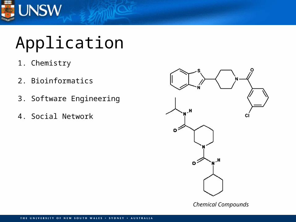
Application1. Chemistry

2. Bioinformatics

3. Software Engineering

4. Social Network

Chemical Compounds

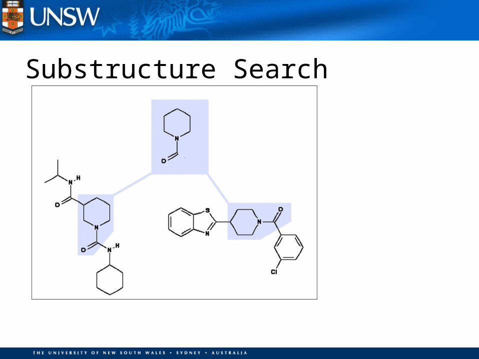
Substructure Search

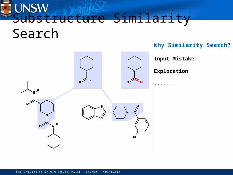
Substructure Similarity Search

Why Similarity Search?

Input Mistake

Exploration

......

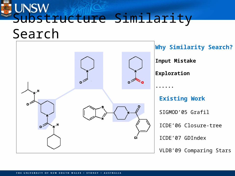
Substructure Similarity Search

Why Similarity Search?

Input Mistake

Exploration

......

Existing Work

SIGMOD’05 Grafil

ICDE’06 Closure-tree

ICDE’07 GDIndex

VLDB’09 Comparing Stars

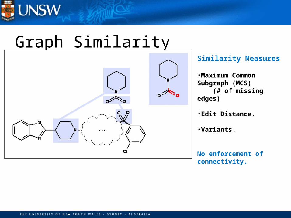
Graph SimilaritySubgraph Similarity Similarity Measures

•Maximum Common Subgraph (MCS) (# of missing edges)

•Edit Distance.

•Variants.

No enforcement ofconnectivity.

Graph Similarity

A New Similarity Measure.

Maximum Connected Common Subgraph – MCCS(counting missing edges while retaining the connectivity)

Graph SimilarityMaximum Connected Common Subgraph – MCCS: Given two graphs g1 and g2, the maximum connected common subgraph of g1 and g2 is the largest connected subgraph of g1 which is subgraph isomorphic to g2, denoted as mccs(g1, g2)

Graph SimilarityMaximum Connected Common Subgraph – MCCS: Given two graphs g1 and g2, the maximum connected common subgraph of g1 and g2 is the largest connected subgraph of g1 which is subgraph isomorphic to g2, denoted as mccs(g1, g2)

Subgraph Distance: Given a query graph q and a data graph g, the Subgraph Distance is defined as,

dist(q, g) = |q| − |mccs(q, g)|The graph size is defined as the number of edges. (# of missing edges from the query)

Graph SimilarityMaximum Connected Common Subgraph – MCCS: Given two graphs g1 and g2, the maximum connected common subgraph of g1 and g2 is the largest connected subgraph of g1 which is subgraph isomorphic to g2, denoted as mccs(g1, g2)

Substructure Similarity Search: Given a graph database D = {g1, g2, ..., gn}, a query graph q, and a subgraph distance threshold , the substructure similarity search is to retrieve all the graphs gi ∈ D with dist(q, gi) ≤ .

Subgraph Distance: Given a query graph q and a data graph g, the Subgraph Distance is defined as,

dist(q, g) = |q| − |mccs(q, g)|The graph size is defined as the number of edges. (# of missing edges from the query)

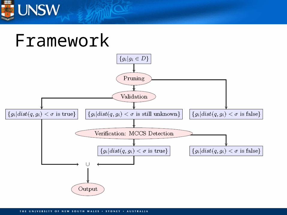
Framework

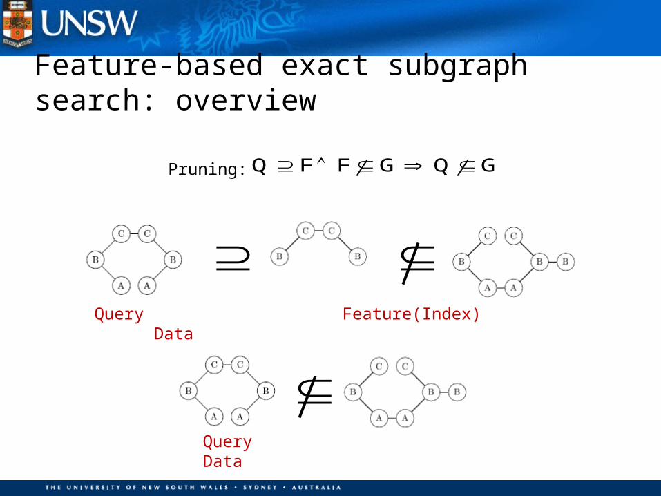
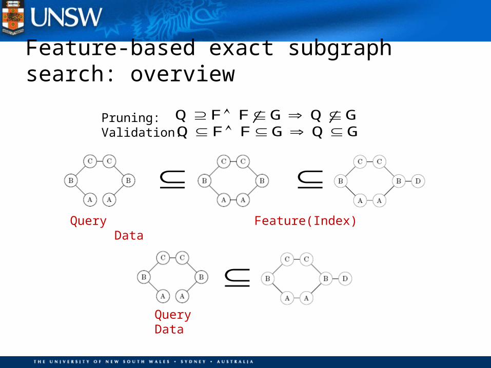
Feature-based exact subgraph search: overview

Query Data

Query Feature(Index) Data

Q F F G Q G Pruning:

Query Data

Query Feature(Index) Data

Q F F G Q G Q F F G Q G

Feature-based exact subgraph search: overview

Pruning:Validation:

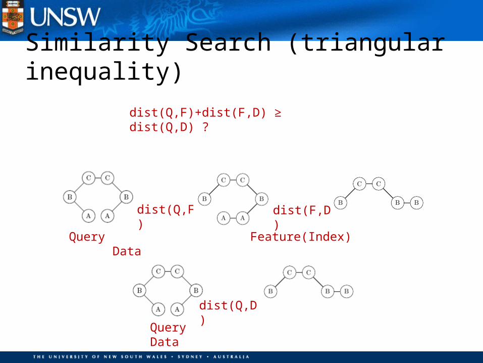
Similarity Search (triangular inequality)

dist(Q,F)+dist(F,D) ≥ dist(Q,D) ?

Query Data

dist(Q,D)

dist(Q,F)

dist(F,D)

Query Feature(Index) Data

Query Data

dist(Q,D)

dist(Q,F)

dist(F,D)

Query Feature(Index) Data

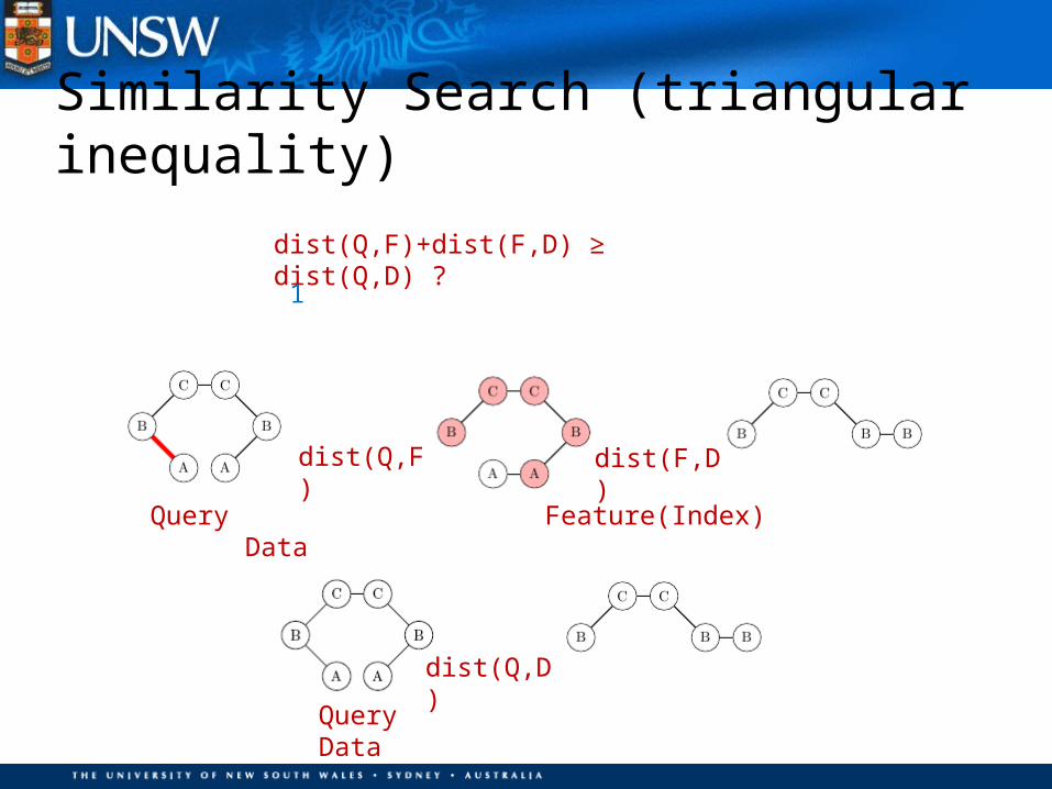
dist(Q,F)+dist(F,D) ≥ dist(Q,D) ?1

Similarity Search (triangular inequality)

Query Data

dist(Q,D)

dist(Q,F)

dist(F,D)

Query Feature(Index) Data

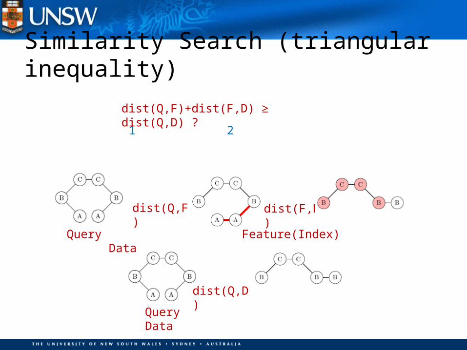
1 2

dist(Q,F)+dist(F,D) ≥ dist(Q,D) ?

Similarity Search (triangular inequality)

Query Data

dist(Q,D)

dist(Q,F)

dist(F,D)

Query Feature(Index) Data

1 2 2

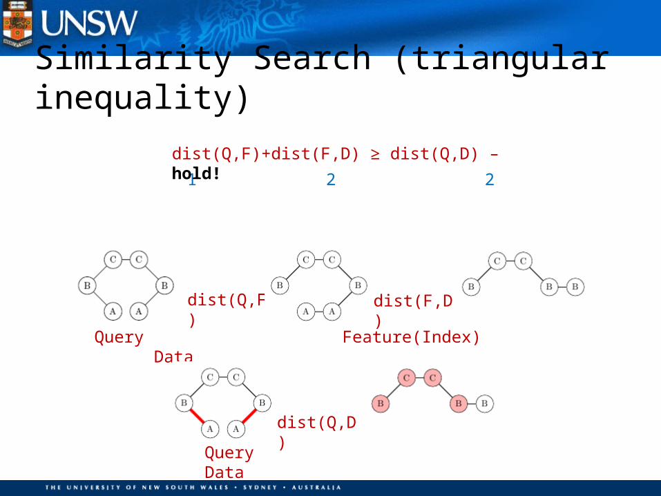
dist(Q,F)+dist(F,D) ≥ dist(Q,D) – hold!

Similarity Search (triangular inequality)

dist(Q,F)

dist(F,D)

0 1 3

Query Feature(Index) Data

Query Data

dist(Q,D)

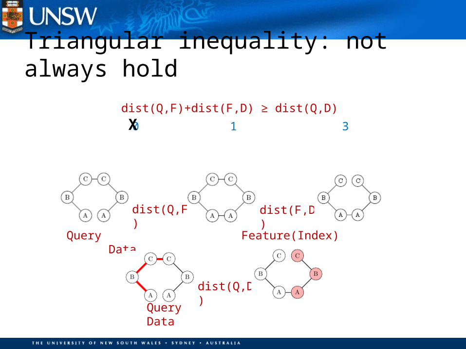
dist(Q,F)+dist(F,D) ≥ dist(Q,D)

X

Triangular inequality: not always hold

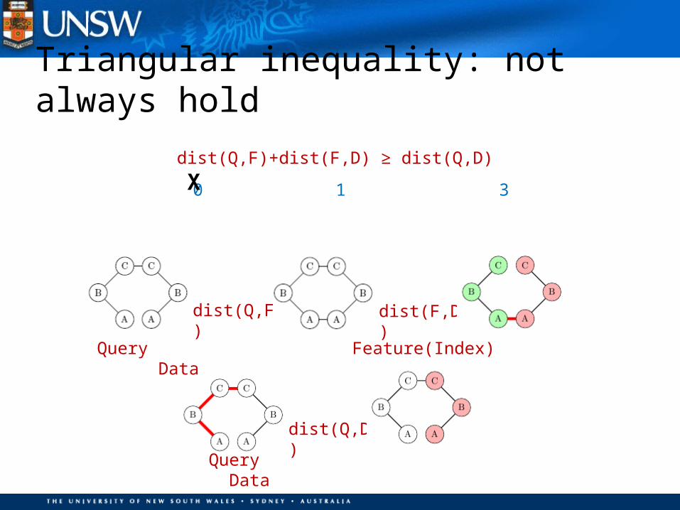
dist(Q,F)

dist(F,D)

0 1 3

Query Feature(Index) Data

Query Data

dist(Q,D)

Triangular inequality: not always hold

dist(Q,F)+dist(F,D) ≥ dist(Q,D)

X

Connectivity DominanceConnectivity Dominance: The connectivity of mccs(g1, g2) dominates the connectivity of g2 if there is a subgraph isomorphic mapping from mccs(g1, g2) to g2 such that if removing all the edges from this mapping, then all the vertices in the embedding mapping are disconnected. (i.e. The removing fully disconnected g2 .)

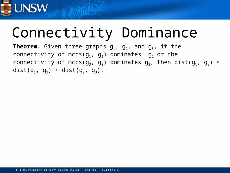
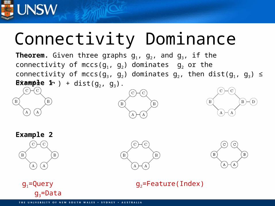
Theorem. Given three graphs g1, g2, and g3, if the connectivity of mccs(g1, g2) dominates g2 or the connectivity of mccs(g3, g2) dominates g2, then dist(g1, g3) ≤ dist(g1, g2) + dist(g2, g3).

Connectivity Dominance

Theorem. Given three graphs g1, g2, and g3, if the connectivity of mccs(g1, g2) dominates g2 or the connectivity of mccs(g3, g2) dominates g2, then dist(g1, g3) ≤ dist(g1, g2) + dist(g2, g3).

Connectivity Dominance

g1=Query g2=Feature(Index) g3=Data

Example 1

Example 2

Theorem. Given three graphs g1, g2, and g3, if the connectivity of mccs(g1, g2) dominates g2 or the connectivity of mccs(g3, g2) dominates g2, then dist(g1, g3) ≤ dist(g1, g2) + dist(g2, g3).

Connectivity Dominance

g1=Query g2=Feature(Index) g3=Data

Example 1

Example 2

mccs(g2,g3) dominates g2

mccs(g1,g2) not dominate g2

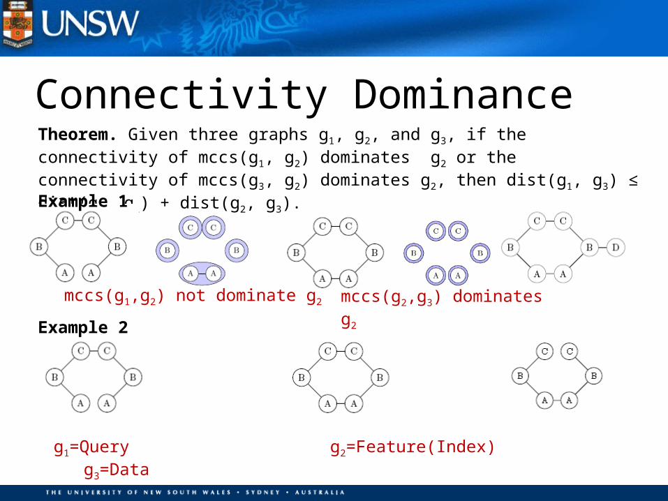
Theorem. Given three graphs g1, g2, and g3, if the connectivity of mccs(g1, g2) dominates g2 or the connectivity of mccs(g3, g2) dominates g2, then dist(g1, g3) ≤ dist(g1, g2) + dist(g2, g3).

Connectivity Dominance

g1=Query g2=Feature(Index) g3=Data

Example 1

Example 2

mccs(g2,g3) dominates g2

mccs(g1,g2) not dominate g2

mccs(g1,g2) not dominate g2 mccs(g2,g3) not dominate g2

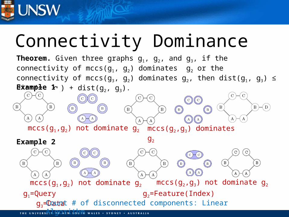
Theorem. Given three graphs g1, g2, and g3, if the connectivity of mccs(g1, g2) dominates g2 or the connectivity of mccs(g3, g2) dominates g2, then dist(g1, g3) ≤ dist(g1, g2) + dist(g2, g3).

Connectivity Dominance

g1=Query g2=Feature(Index) g3=Data

Example 1

Example 2

mccs(g2,g3) dominates g2

Count # of disconnected components: Linear Algorithm

mccs(g1,g2) not dominate g2

mccs(g1,g2) not dominate g2 mccs(g2,g3) not dominate g2

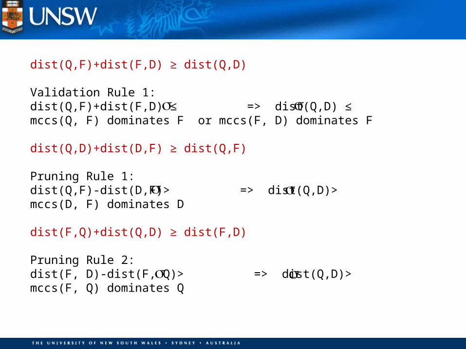
dist(Q,F)+dist(F,D) ≥ dist(Q,D)

Validation Rule 1:dist(Q,F)+dist(F,D) ≤ => dist(Q,D) ≤mccs(Q, F) dominates F or mccs(F, D) dominates F

dist(Q,D)+dist(D,F) ≥ dist(Q,F)

Pruning Rule 1:dist(Q,F)-dist(D,F)> => dist(Q,D)>mccs(D, F) dominates D

dist(F,Q)+dist(Q,D) ≥ dist(F,D)

Pruning Rule 2:dist(F, D)-dist(F, Q)> => dist(Q,D)>mccs(F, Q) dominates Q

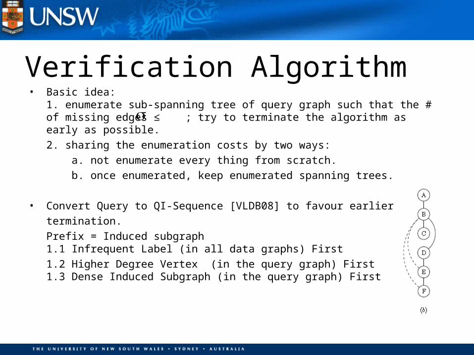
• Basic idea:1. enumerate sub-spanning tree of query graph such that the # of missing edges ≤ ; try to terminate the algorithm as early as possible.2. sharing the enumeration costs by two ways: a. not enumerate every thing from scratch. b. once enumerated, keep enumerated spanning trees.

• Convert Query to QI-Sequence [VLDB08] to favour earlier termination.Prefix = Induced subgraph1.1 Infrequent Label (in all data graphs) First1.2 Higher Degree Vertex  (in the query graph) First1.3 Dense Induced Subgraph (in the query graph) First   

Verification Algorithm

Verification Algorithm

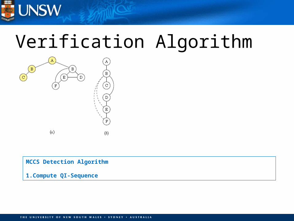
MCCS Detection Algorithm

1.Compute QI-Sequence

Verification Algorithm

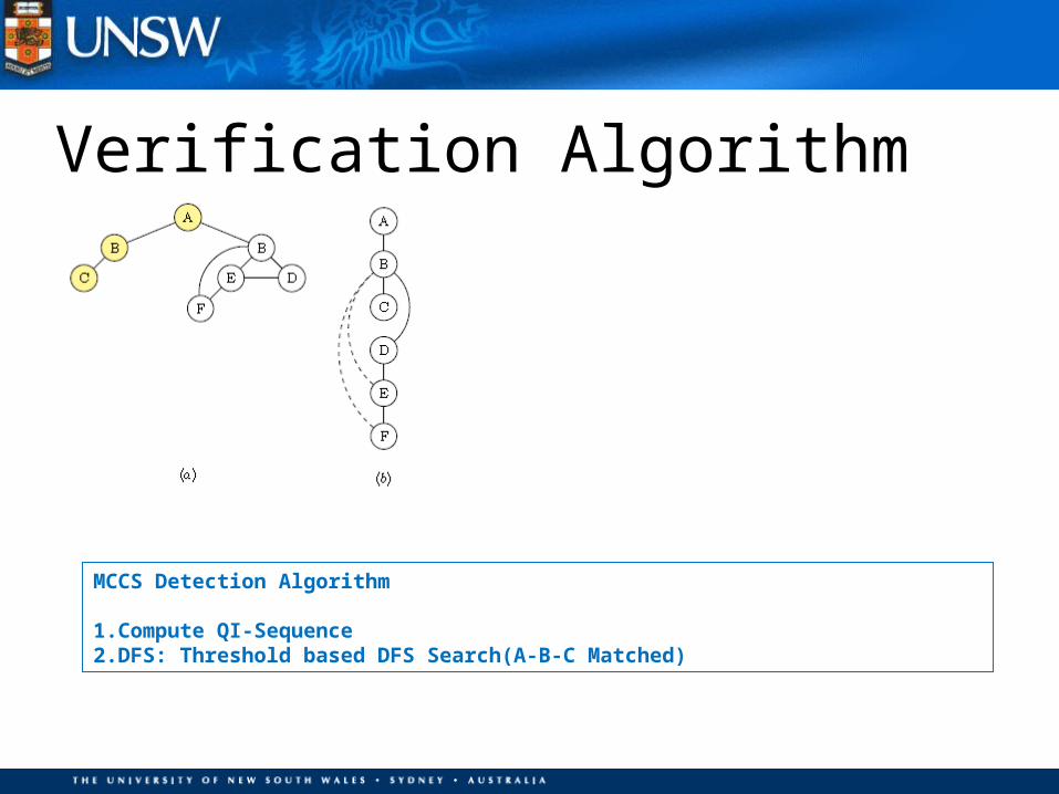
MCCS Detection Algorithm

1.Compute QI-Sequence2.DFS: Threshold based DFS Search(A-B-C Matched)

Verification Algorithm

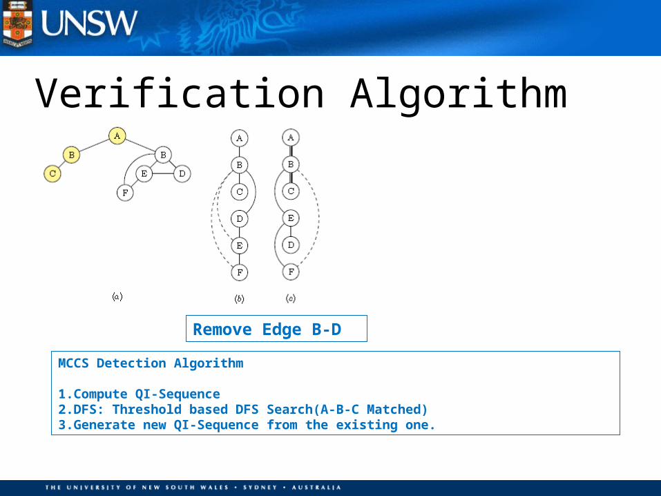
Remove Edge B-D

MCCS Detection Algorithm

1.Compute QI-Sequence2.DFS: Threshold based DFS Search(A-B-C Matched)3.Generate new QI-Sequence from the existing one.

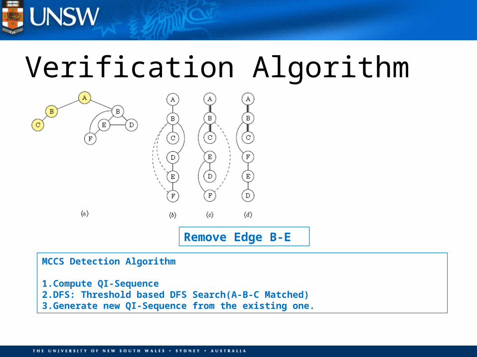
Verification Algorithm

Remove Edge B-E

MCCS Detection Algorithm

1.Compute QI-Sequence2.DFS: Threshold based DFS Search(A-B-C Matched)3.Generate new QI-Sequence from the existing one.

Verification Algorithm

Remove Edge B-F

MCCS Detection Algorithm

1.Compute QI-Sequence2.DFS: Threshold based DFS Search(A-B-C Matched)3.Generate new QI-Sequence from the existing one.

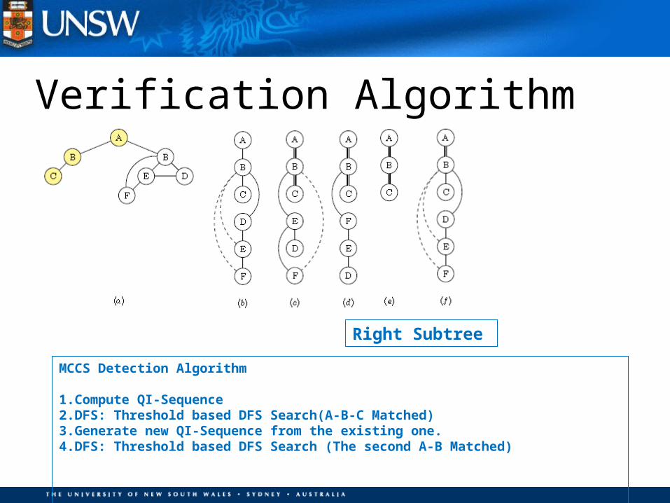
Verification Algorithm

Right Subtree

MCCS Detection Algorithm

1.Compute QI-Sequence2.DFS: Threshold based DFS Search(A-B-C Matched)3.Generate new QI-Sequence from the existing one.4.DFS: Threshold based DFS Search (The second A-B Matched)

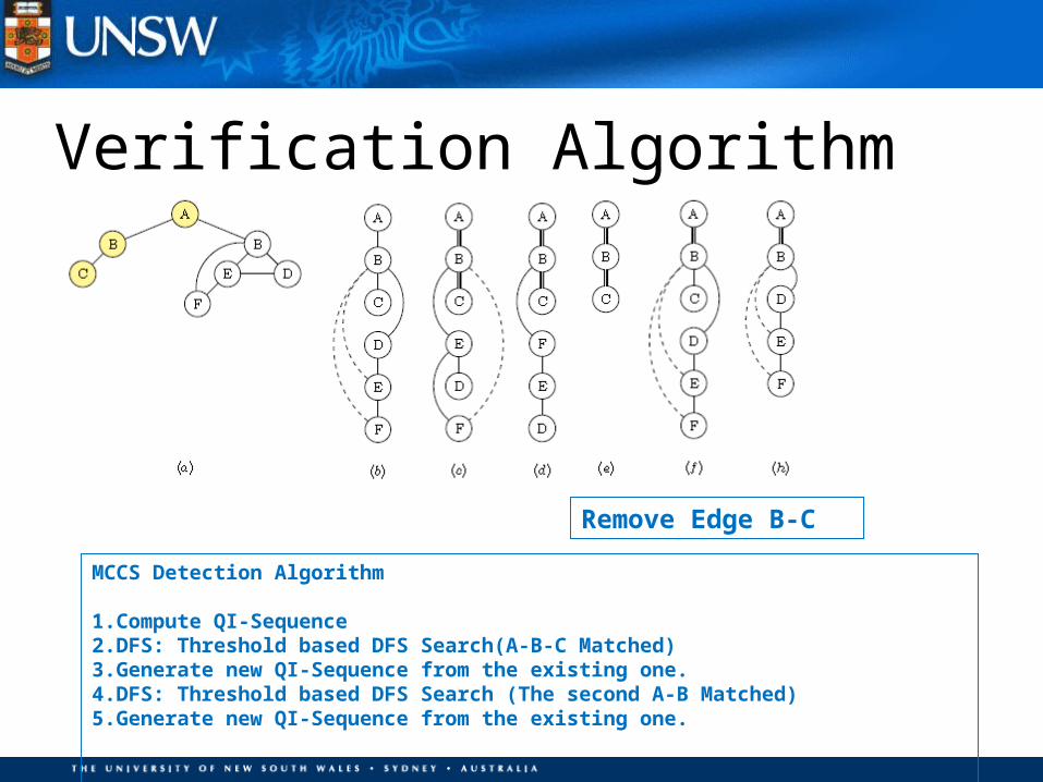
Verification Algorithm

Remove Edge B-C

MCCS Detection Algorithm

1.Compute QI-Sequence2.DFS: Threshold based DFS Search(A-B-C Matched)3.Generate new QI-Sequence from the existing one.4.DFS: Threshold based DFS Search (The second A-B Matched)5.Generate new QI-Sequence from the existing one.

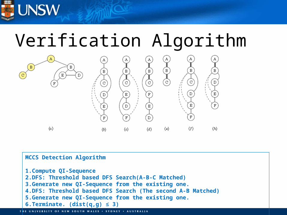
Verification Algorithm

MCCS Detection Algorithm

1.Compute QI-Sequence2.DFS: Threshold based DFS Search(A-B-C Matched)3.Generate new QI-Sequence from the existing one.4.DFS: Threshold based DFS Search (The second A-B Matched)5.Generate new QI-Sequence from the existing one.6.Terminate. (dist(q,g) ≤ 3)

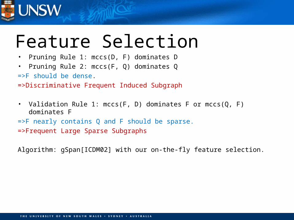
Feature Selection• Pruning Rule 1: mccs(D, F) dominates D• Pruning Rule 2: mccs(F, Q) dominates Q=>F should be dense.=>Discriminative Frequent Induced Subgraph

• Validation Rule 1: mccs(F, D) dominates F or mccs(Q, F) dominates F

=>F nearly contains Q and F should be sparse.=>Frequent Large Sparse Subgraphs

Algorithm: gSpan[ICDM02] with our on-the-fly feature selection.

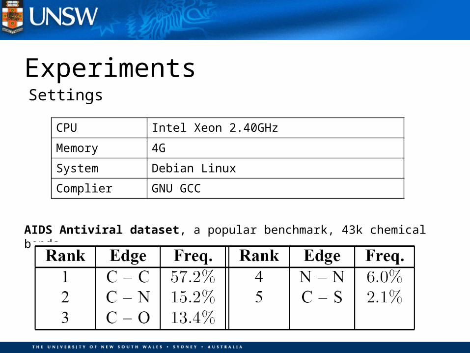
ExperimentsSettings

CPU Intel Xeon 2.40GHz

Memory 4G

System Debian Linux

Complier GNU GCC

AIDS Antiviral dataset, a popular benchmark, 43k chemical bonds

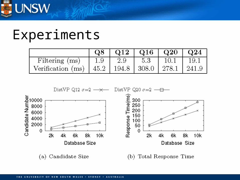
Experiments

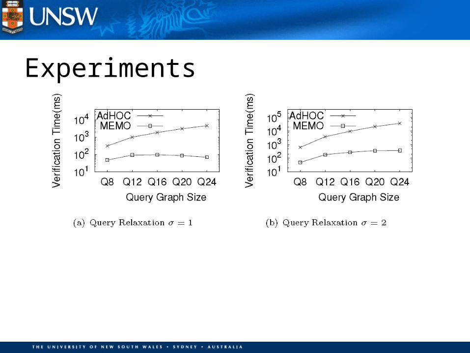
Experiments

Conclusion

Thanks

Connected Substructure Similarity Search

1.Measure: Maximum Connected Common Subgraph – MCCS

2.Connectivity Dominance => Triangular inequality

3.MCCS Detection Algorithm

(Index, Filtering & Validation, Verification Techniques)

Future Work:

Large Graphs? New Measures?