connecting rod shape optimization tutorial (autodesign)...connecting rod shape optimization this...
TRANSCRIPT

Connecting Rod Shape
Optimization Tutorial
(AutoDesign)
Copyright © 2019 FunctionBay, Inc. All rights reserved.
User and training documentation from FunctionBay, Inc. is subjected to the copyright laws of
the Republic of Korea and other countries and is provided under a license agreement that
restricts copying, disclosure, and use of such documentation. FunctionBay, Inc. hereby grants
to the licensed user the right to make copies in printed form of this documentation if provided
on software media, but only for internal/personal use and in accordance with the license
agreement under which the applicable software is licensed. Any copy made shall include the
FunctionBay, Inc. copyright notice and any other proprietary notice provided by FunctionBay,
Inc. This documentation may not be disclosed, transferred, modified, or reduced to any form,
including electronic media, or transmitted or made publicly available by any means without
the prior written consent of FunctionBay, Inc. and no authorization is granted to make copies
for such purpose.
Information described herein is furnished for general information only, is subjected to change
without notice, and should not be construed as a warranty or commitment by FunctionBay,
Inc. FunctionBay, Inc. assumes no responsibility or liability for any errors or inaccuracies that
may appear in this document.
The software described in this document is provided under written license agreement,
contains valuable trade secrets and proprietary information, and is protected by the copyright
laws of the Republic of Korea and other countries. UNAUTHORIZED USE OF SOFTWARE OR
ITS DOCUMENTATION CAN RESULT IN CIVIL DAMAGES AND CRIMINAL PROSECUTION.
Registered Trademarks of FunctionBay, Inc. or Subsidiary
RecurDyn is a registered trademark of FunctionBay, Inc.
RecurDyn/Professional, RecurDyn/ProcessNet, RecurDyn/Acoustics, RecurDyn/AutoDesign,
RecurDyn/Bearing, RecurDyn/Belt, RecurDyn/Chain, RecurDyn/CoLink, RecurDyn/Control,
RecurDyn/Crank, RecurDyn/Durability, RecurDyn/EHD, RecurDyn/Engine,
RecurDyn/eTemplate, RecurDyn/FFlex, RecurDyn/Gear, RecurDyn/DriveTrain,
RecurDyn/HAT, RecurDyn/Linear, RecurDyn/Mesher, RecurDyn/MTT2D, RecurDyn/MTT3D,
RecurDyn/Particleworks I/F, RecurDyn/Piston, RecurDyn/R2R2D, RecurDyn/RFlex,
RecurDyn/RFlexGen, RecurDyn/SPI, RecurDyn/Spring, RecurDyn/TimingChain,
RecurDyn/Tire, RecurDyn/Track_HM, RecurDyn/Track_LM, RecurDyn/TSG, RecurDyn/Valve
are trademarks of FunctionBay, Inc.
Edition Note
This document describes the release information of RecurDyn V9R3.

Table of Contents
Connecting Rod Shape Optimization ........................................... 1
Loading and simulation the model ............................................. 2
Defining the design variables and setting .................................... 4
Defining the analysis responses ................................................ 12
Running a design optimization .................................................. 13
Comparison of analysis results ................................................. 16

C O N N E C T I N G R O D S H A P E O P T I M I Z A T I O N T U T O R I A L ( A U T O D E S I G N )
1
Connecting Rod Shape
Optimization
This tutorials deal with the shape optimization design problem. Design target is a connecting
rod in engine. Connecting rod function is a transferred reciprocating movement of the piston
to crankshaft rotational movement. Therefore, design goal is a minimize mass for energy
efficiency and reduce inertial force. Also a design constraint is strength to withstand
compressive forces of piston. Design variable select the shape on connecting rod.
Note: If you change the file path at discretion, it can be located in any folder that you specify.
Sample
G
Open files related in Sample-G
Sample <Install Dir>
\Help\Tutorial\AutoDesign\AutoDesign_G\Examples\Sample_G.rdyn
Solution <Install Dir>
\Help\Tutorial\AutoDesign\AutoDesign_G\Solutions\Sample_G.rdyn

C O N N E C T I N G R O D S H A P E O P T I M I Z A T I O N T U T O R I A L ( A U T O D E S I G N )
2
Loading and simulation the
model
1. On your Desktop, double-click the RecurDyn icon.
RecurDyn starts and the Start RecurDyn dialog box appears.
2. Close Start RecurDyn dialog box. You will
use an existing model.
3. In the Quick Access toolbar, click the Open
tool and select ‘Sample_G.rdyn’ from the
same directory where this tutorial is located.
The system appears on the screen.
Chapter
1
C O N N E C T I N G R O D S H A P E O P T I M I Z A T I O N T U T O R I A L ( A U T O D E S I G N )
3
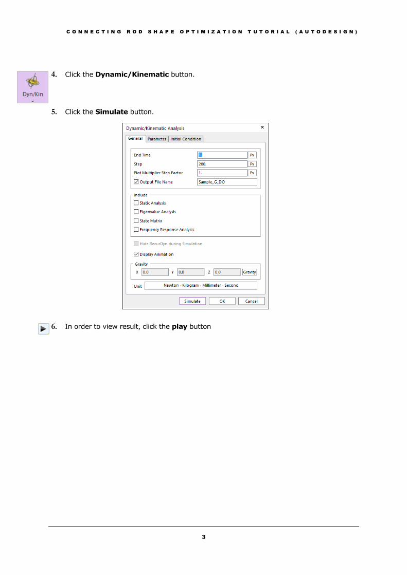
4. Click the Dynamic/Kinematic button.
5. Click the Simulate button.
6. In order to view result, click the play button

C O N N E C T I N G R O D S H A P E O P T I M I Z A T I O N T U T O R I A L ( A U T O D E S I G N )
4
Defining the design variables
and setting
In the figure, design variable selects connecting road shape. Design variables divide into 4
design variable zones. And, DV1 is a radius in zone C and DV2 is radius in zone A. DV3 and 4
is a width in zone B. DV 5 and 6 is a height in zone D.
Chapter
2
Zone A Zone B Zone C
DV 2
DV 4
DV 1
To
p v
iew
Sid
e v
iew
Zone D
DV 3
DV 5
DV 6
C O N N E C T I N G R O D S H A P E O P T I M I Z A T I O N T U T O R I A L ( A U T O D E S I G N )
5
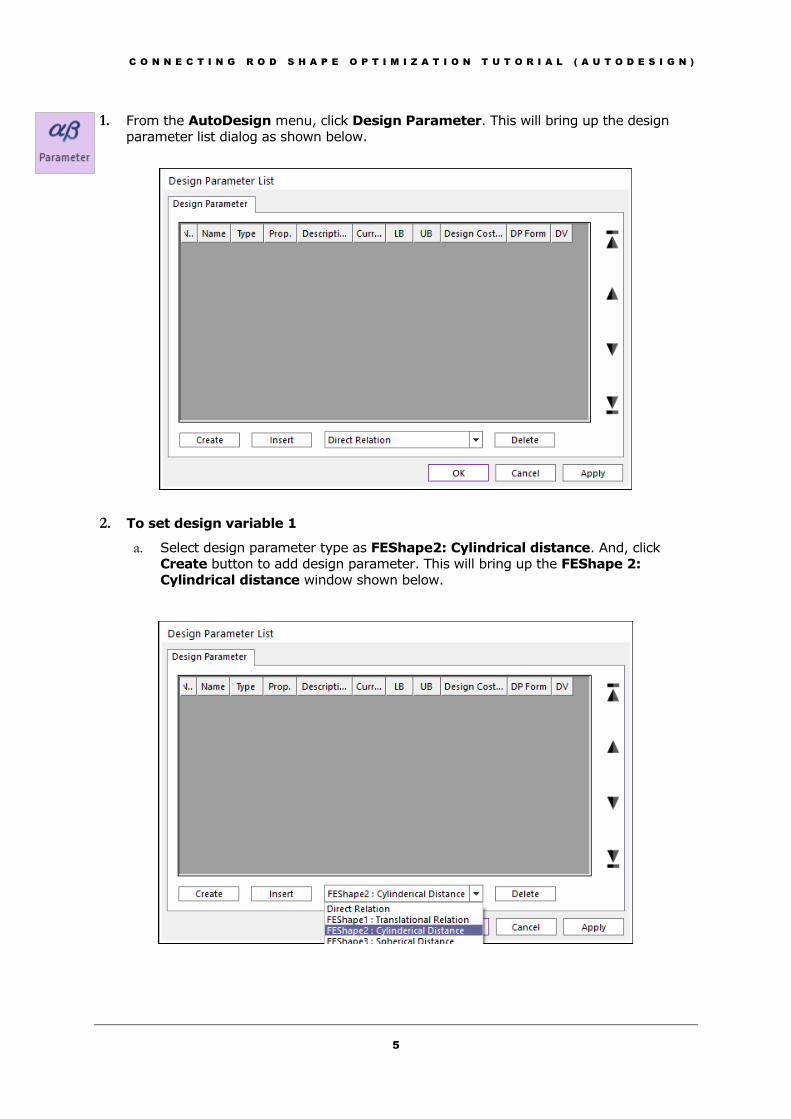
1. From the AutoDesign menu, click Design Parameter. This will bring up the design
parameter list dialog as shown below.
2. To set design variable 1
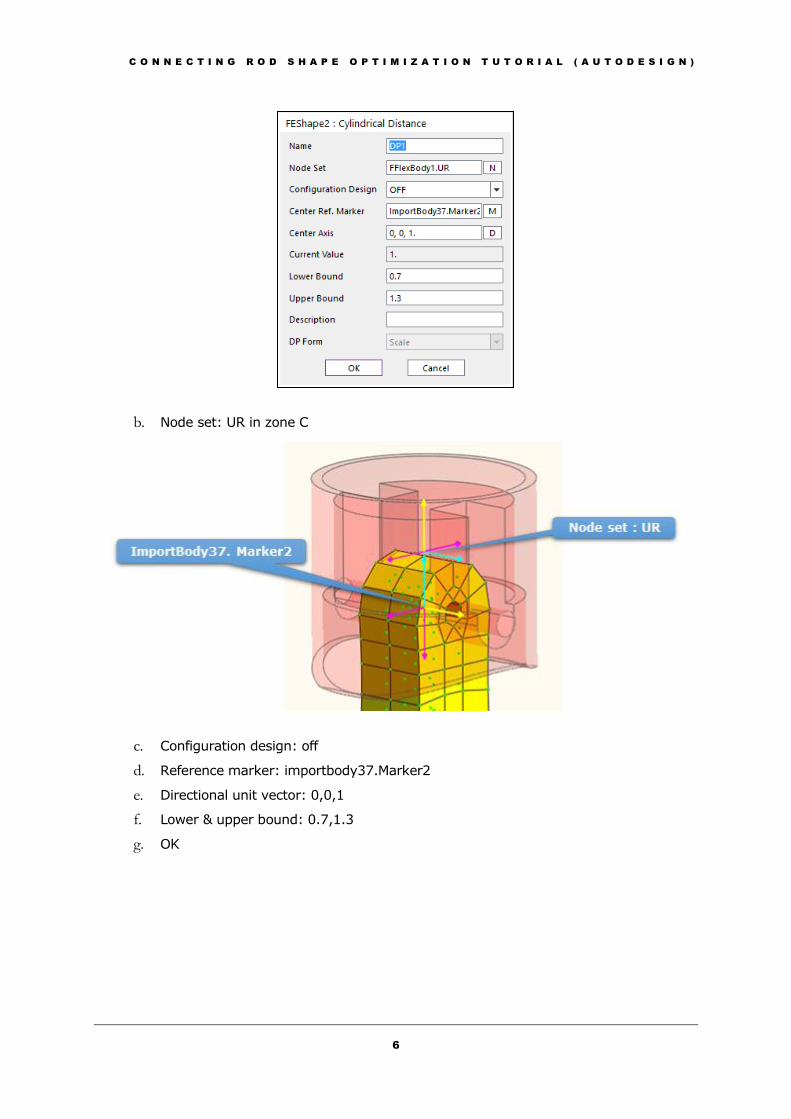
a. Select design parameter type as FEShape2: Cylindrical distance. And, click
Create button to add design parameter. This will bring up the FEShape 2:
Cylindrical distance window shown below.
C O N N E C T I N G R O D S H A P E O P T I M I Z A T I O N T U T O R I A L ( A U T O D E S I G N )
6
b. Node set: UR in zone C
c. Configuration design: off
d. Reference marker: importbody37.Marker2
e. Directional unit vector: 0,0,1
f. Lower & upper bound: 0.7,1.3
g. OK

C O N N E C T I N G R O D S H A P E O P T I M I Z A T I O N T U T O R I A L ( A U T O D E S I G N )
7
3. To set design variable 2
a. Select design parameter type as FEShape 2: Cylindrical distance. And, click
Create button to add design parameter.
b. Node set: BR in zone A
c. Configuration design: off
d. Reference marker: importbody3.Marker2
e. Directional unit vector: 0,0,1
f. Lower & upper bound: 0.8,1.2
g. OK
C O N N E C T I N G R O D S H A P E O P T I M I Z A T I O N T U T O R I A L ( A U T O D E S I G N )
8
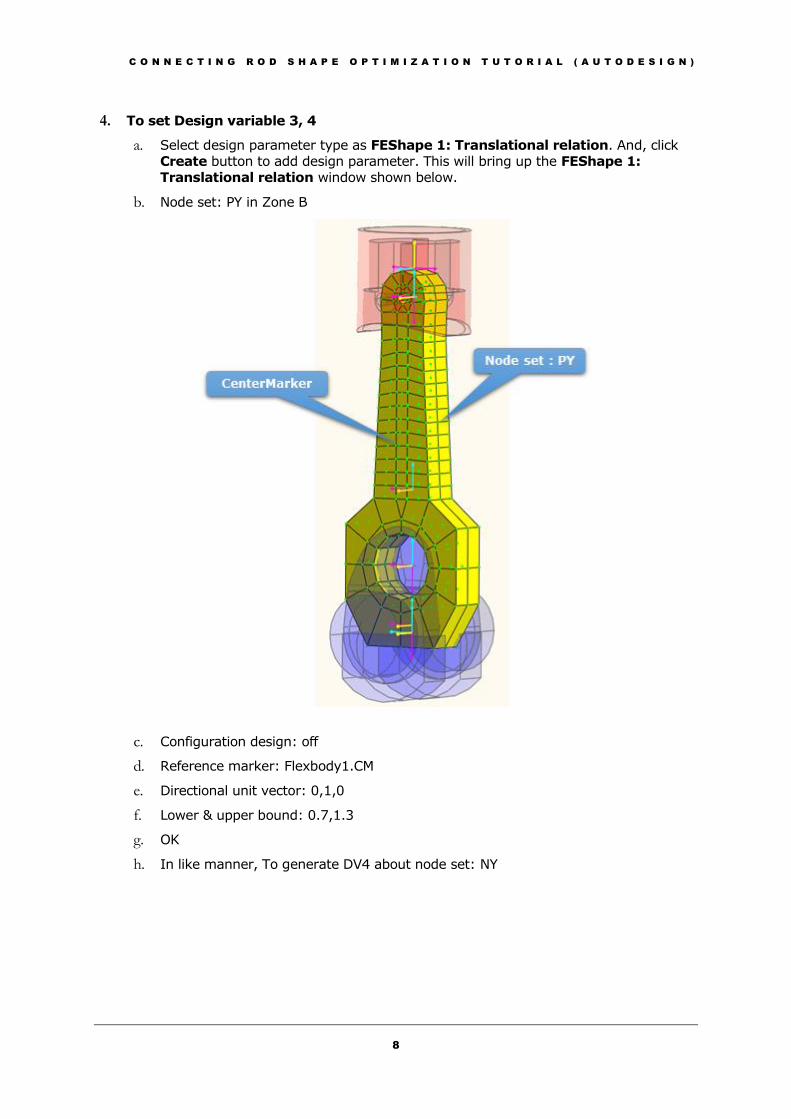
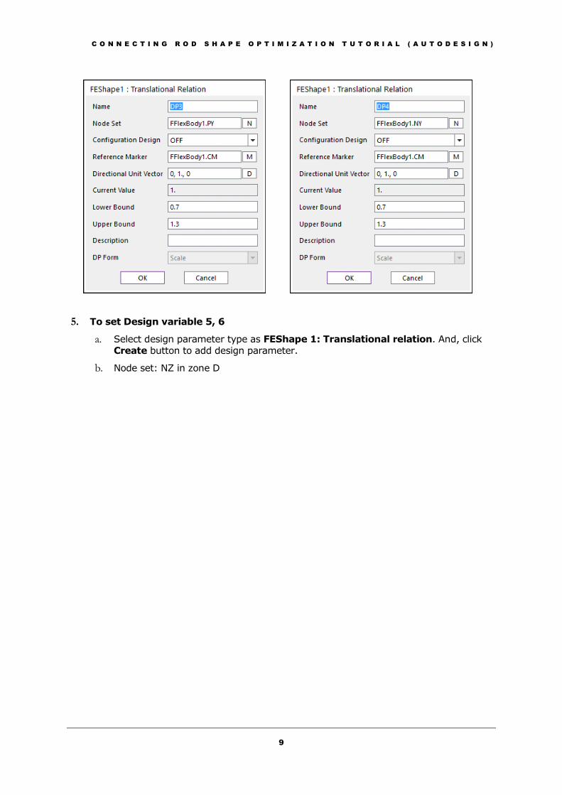
4. To set Design variable 3, 4
a. Select design parameter type as FEShape 1: Translational relation. And, click
Create button to add design parameter. This will bring up the FEShape 1:
Translational relation window shown below.
b. Node set: PY in Zone B
c. Configuration design: off
d. Reference marker: Flexbody1.CM
e. Directional unit vector: 0,1,0
f. Lower & upper bound: 0.7,1.3
g. OK
h. In like manner, To generate DV4 about node set: NY
C O N N E C T I N G R O D S H A P E O P T I M I Z A T I O N T U T O R I A L ( A U T O D E S I G N )
9
5. To set Design variable 5, 6
a. Select design parameter type as FEShape 1: Translational relation. And, click
Create button to add design parameter.
b. Node set: NZ in zone D

C O N N E C T I N G R O D S H A P E O P T I M I Z A T I O N T U T O R I A L ( A U T O D E S I G N )
10
c. Configuration design: off
d. Reference marker: Flexbody.CM
e. Directional unit vector: 0,0,1
f. Lower & upper bound: 0.6,1.4
g. OK
h. In like manner, To generate DV6 about node set: PZ

C O N N E C T I N G R O D S H A P E O P T I M I Z A T I O N T U T O R I A L ( A U T O D E S I G N )
11
C O N N E C T I N G R O D S H A P E O P T I M I Z A T I O N T U T O R I A L ( A U T O D E S I G N )
12
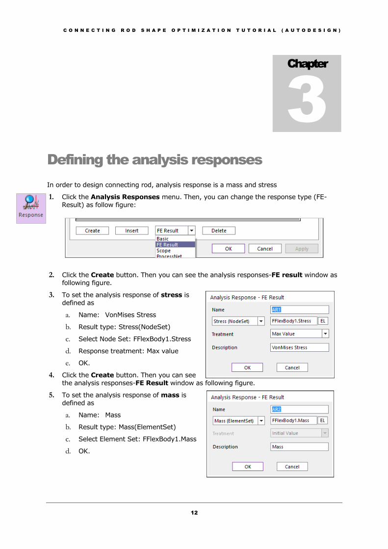
Defining the analysis responses
In order to design connecting rod, analysis response is a mass and stress
1. Click the Analysis Responses menu. Then, you can change the response type (FE-
Result) as follow figure:
2. Click the Create button. Then you can see the analysis responses-FE result window as
following figure.
3. To set the analysis response of stress is
defined as
a. Name: VonMises Stress
b. Result type: Stress(NodeSet)
c. Select Node Set: FFlexBody1.Stress
d. Response treatment: Max value
e. OK.
4. Click the Create button. Then you can see
the analysis responses-FE Result window as following figure.
5. To set the analysis response of mass is
defined as
a. Name: Mass
b. Result type: Mass(ElementSet)
c. Select Element Set: FFlexBody1.Mass
d. OK.
Chapter
3

C O N N E C T I N G R O D S H A P E O P T I M I Z A T I O N T U T O R I A L ( A U T O D E S I G N )
13
Running a design optimization
The optimization problem is defined as:
Minimize the mass of the connecting rod
Subject to
▪ The stress =< Limit value
1. Click the Design Optimization menu. Then, you can see the design variable list as
following figure:
2. Click the Performance Index tab. Then, you can see the following list. If this window is
empty, then you create the following Pls.
Chapter
4
C O N N E C T I N G R O D S H A P E O P T I M I Z A T I O N T U T O R I A L ( A U T O D E S I G N )
14
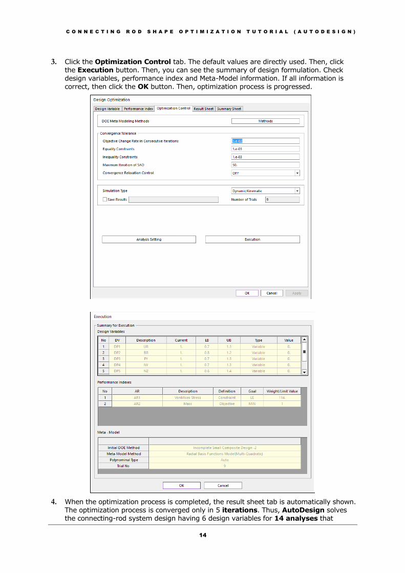
3. Click the Optimization Control tab. The default values are directly used. Then, click
the Execution button. Then, you can see the summary of design formulation. Check
design variables, performance index and Meta-Model information. If all information is
correct, then click the OK button. Then, optimization process is progressed.
4. When the optimization process is completed, the result sheet tab is automatically shown.
The optimization process is converged only in 5 iterations. Thus, AutoDesign solves
the connecting-rod system design having 6 design variables for 14 analyses that
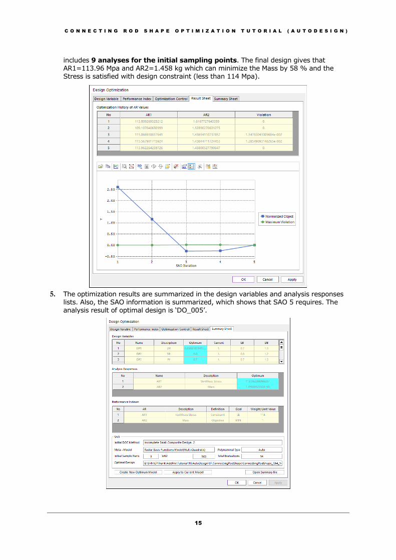
C O N N E C T I N G R O D S H A P E O P T I M I Z A T I O N T U T O R I A L ( A U T O D E S I G N )
15
includes 9 analyses for the initial sampling points. The final design gives that
AR1=113.96 Mpa and AR2=1.458 kg which can minimize the Mass by 58 % and the
Stress is satisfied with design constraint (less than 114 Mpa).
5. The optimization results are summarized in the design variables and analysis responses
lists. Also, the SAO information is summarized, which shows that SAO 5 requires. The
analysis result of optimal design is ‘DO_005’.
C O N N E C T I N G R O D S H A P E O P T I M I Z A T I O N T U T O R I A L ( A U T O D E S I G N )
16
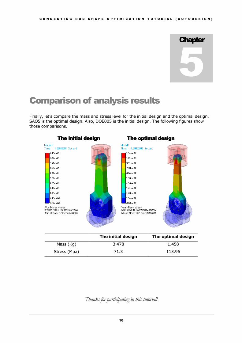
Comparison of analysis results
Finally, let’s compare the mass and stress level for the initial design and the optimal design.
SAO5 is the optimal design. Also, DOE005 is the initial design. The following figures show
those comparisons.
The initial design The optimal design
Mass (Kg) 3.478 1.458
Stress (Mpa) 71.3 113.96
Thanks for participating in this tutorial!
Chapter
5
The initial design The optimal design