Connection Between Alignment and HMMs

A state model for alignment

-AGGCTATCACCTGACCTCCAGGCCGA--TGCCC---TAG-CTATCAC--GACCGC-GGTCGATTTGCCCGACCIMMJMMMMMMMJJMMMMMMJMMMMMMMIIMMMMMIII

M(+1,+1)

I(+1, 0)

J(0, +1)

Alignments correspond 1-to-1 with sequences of states M, I, J

Let’s score the transitions

-AGGCTATCACCTGACCTCCAGGCCGA--TGCCC---TAG-CTATCAC--GACCGC-GGTCGATTTGCCCGACCIMMJMMMMMMMJJMMMMMMJMMMMMMMIIMMMMMIII

M(+1,+1)

I(+1, 0)

J(0, +1)

Alignments correspond 1-to-1 with sequences of states M, I, J

s(xi, yj)

s(xi, yj) s(xi, yj)

-d -d

-e -e

-e

-e

How do we find optimal alignment according to this model?

Dynamic Programming:

M(i, j): Optimal alignment of x1…xi to y1…yj ending in M

I(i, j): Optimal alignment of x1…xi to y1…yj ending in I

J(i, j): Optimal alignment of x1…xi to y1…yj ending in J

The score is additive, therefore we can apply DP recurrence formulas

Needleman Wunsch with affine gaps – state version

Initialization:M(0,0) = 0; M(i,0) = M(0,j) = -, for i, j > 0I(i,0) = d + ie; J(0,j) = d + je

Iteration:

M(i – 1, j – 1)M(i, j) = s(xi, yj) + max I(i – 1, j – 1)

J(i – 1, j – 1)

e + I(i – 1, j)I(i, j) = max e + J(i, j – 1)

d + M(i – 1, j – 1)

e + I(i – 1, j)J(i, j) = max e + J(i, j – 1)

d + M(i – 1, j – 1)

Termination:Optimal alignment given by max { M(m, n), I(m, n), J(m, n) }

Probabilistic interpretation of an alignment

An alignment is a hypothesis that the two sequences are related by evolution

Goal:

Produce the most likely alignment

Assert the likelihood that the sequences are indeed related

A Pair HMM for alignments

MP(xi, yj)

IP(xi)

JP(yj)

1 – 2 –

1 – 2 –

1 – 2 –

BEGIN

END

M JI

1 – 2 –

A Pair HMM for not aligned sequences

BEGIN IP(xi)

ENDBEGIN

JP(yj)

END1 -

1 -

1 -

1 -

P(x, y | R) = (1 – )m P(x1)…P(xm) (1 – )n P(y1)…P(yn)

= 2(1 – )m+n i P(xi) j P(yj)

Model R

To compare ALIGNMENT vs. RANDOM hypothesis

Every pair of letters contributes:

• (1 – 2 – ) P(xi, yj) when matched

P(xi) P(yj) when gapped

• (1 – )2 P(xi) P(yj) in random model

Focus on comparison of

P(xi, yj) vs. P(xi) P(yj)

BEGINI

P(xi)END

BEGINJ

P(yj)END

1 -

1 -

1 -

1 -

MP(xi, yj)

IP(xi)

JP(yj)

1 – 2 –

1 – 2 –

1 – 2 –

To compare ALIGNMENT vs. RANDOM hypothesis

Idea:We will divide alignment score by the random score, and take logarithms

Let P(xi, yj) (1 – 2 – )

s(xi, yj) = log ––––––––––– + log ––––––––––– P(xi) P(yj) (1 – )2

(1 – 2 – ) P(xi) d = – log ––––––––––––––––––––

(1 – ) (1 – 2 – ) P(xi)

P(xi) e = – log –––––––––––

(1 – ) P(xi)

Every letter b in random model contributes (1 – ) P(b)

The meaning of alignment scores

Because , , are small, and , are very small,

P(xi, yj) (1 – 2 – ) P(xi, yj)

s(xi, yj) = log ––––––––– + log –––––––––– log –––––––– + log(1 – 2)

P(xi) P(yj) (1 – )2 P(xi) P(yj)

(1 – – ) 1 – d = – log –––––––––––––––––– – log ––––––

(1 – ) (1 – 2 – ) 1 – 2

e = – log ––––––– – log

(1 – )

The meaning of alignment scores

• The Viterbi algorithm for Pair HMMs corresponds exactly to the Needleman-Wunsch algorithm with affine gaps

• However, now we need to score alignment with parameters that add up to probability distributions

1/mean arrival time of next gap 1/mean length of next gap

affine gaps decouple arrival time with length

1/mean length of conserved segments (set to ~0) 1/mean length of sequences of interest (set to ~0)

The meaning of alignment scores

Match/mismatch scores: P(xi, yj)

s(a, b) log ––––––––––– (let’s ignore log(1 – 2) for the moment – assume no gaps)

P(xi) P(yj)

Example:Say DNA regions between human and mouse have average conservation of 50%

Then P(A,A) = P(C,C) = P(G,G) = P(T,T) = 1/8 (so they sum to ½) P(A,C) = P(A,G) =……= P(T,G) = 1/24 (24 mismatches, sum to ½)

Say P(A) = P(C) = P(G) = P(T) = ¼

log [ (1/8) / (1/4 * 1/4) ] = log 2 = 1, for matchThen, s(a, b) = log [ (1/24) / (1/4 * 1/4) ] = log 16/24 = -0.585

Note: 0.585 / 1.585 = 37.5

According to this model, a 37.5%-conserved sequence with no gaps would score on average 0.375 * 1 – 0.725 * 0.585 = 0

Why? 37.5% is between the 50% conservation model, and the random 25% conservation model !

Substitution matrices

A more meaningful way to assign match/mismatch scores

For protein sequences, different substitutions have dramatically different frequencies!

BLOSUM matrices:

1. Start from BLOCKS database (curated, gap-free alignments)

2. Cluster sequences according to > X% identity

3. Calculate Aab: # of aligned a-b in distinct clusters, correcting by 1/mn, where m, n are the two cluster sizes

4. Estimate

P(a) = (b Aab)/(c≤d Acd); P(a, b) = Aab/(c≤d Acd)

BLOSUM matrices

BLOSUM 50 BLOSUM 62

(The two are scaled differently)

DNA Sequencing

Next few topics

• DNA Sequencing Sequencing strategies

• Hierarchical• Online (Walking)• Whole Genome Shotgun

Sequencing Assembly

• Gene Recognition The GENSCAN hidden Markov model Comparative Gene Recognition – Twinscan, SLAM

• Large-scale and multiple sequence alignment

• Microarrays, Regulation, and Motif-finding

• Evolution and Phylogeny

• RNA Structure and Modeling

New topic: DNA sequencing

How we obtain the sequence of nucleotides of a species

…ACGTGACTGAGGACCGTGCGACTGAGACTGACTGGGTCTAGCTAGACTACGTTTTATATATATATACGTCGTCGTACTGATGACTAGATTACAGACTGATTTAGATACCTGACTGATTTTAAAAAAATATT…

Which representative of the species?

Which human?

Answer one:

Answer two: it doesn’t matter

Polymorphism rate: number of letter changes between two different members of a species

Humans: ~1/1,000

Other organisms have much higher polymorphism rates

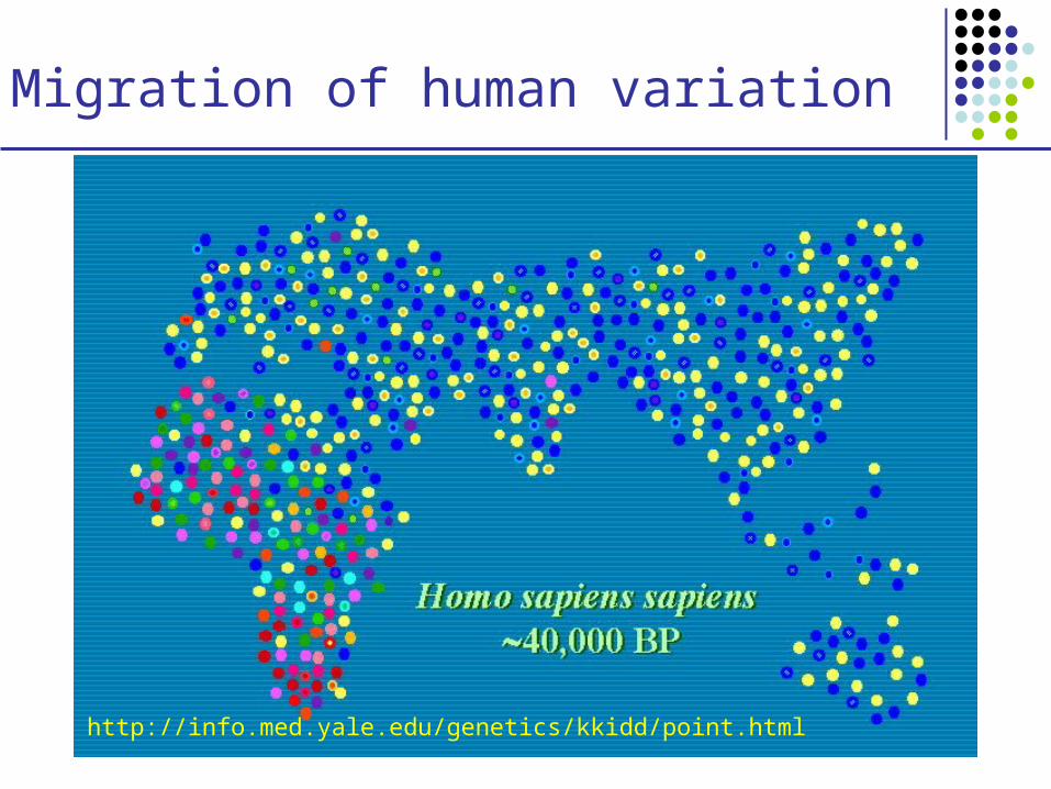
Why humans are so similar

A small population that interbred reduced the genetic variation

Out of Africa ~ 100,000 years ago

Out of Africa

Migration of human variation

http://info.med.yale.edu/genetics/kkidd/point.html

Migration of human variation

http://info.med.yale.edu/genetics/kkidd/point.html

Migration of human variation

http://info.med.yale.edu/genetics/kkidd/point.html

DNA Sequencing

Goal:

Find the complete sequence of A, C, G, T’s in DNA

Challenge:

There is no machine that takes long DNA as an input, and gives the complete sequence as output

Can only sequence ~500 letters at a time

DNA sequencing – vectors

+ =

DNA

Shake

DNA fragments

VectorCircular genome(bacterium, plasmid)

Knownlocation

(restrictionsite)

Different types of vectors

VECTOR Size of insert

Plasmid2,000-10,000

Can control the size

Cosmid 40,000

BAC (Bacterial Artificial Chromosome)

70,000-300,000

YAC (Yeast Artificial Chromosome)

> 300,000

Not used much recently

DNA sequencing – gel electrophoresis

1. Start at primer(restriction site)

2. Grow DNA chain

3. Include dideoxynucleoside (modified a, c, g, t)

4. Stops reaction at all possible points

5. Separate products with length, using gel electrophoresis

Electrophoresis diagrams

Challenging to read answer

Challenging to read answer

Challenging to read answer

Reading an electropherogram

1. Filtering

2. Smoothening

3. Correction for length compressions

4. A method for calling the letters – PHRED

PHRED – PHil’s Read EDitor (by Phil Green)Based on dynamic programming

Several better methods exist, but labs are reluctant to change

Output of PHRAP: a read

A read: 500-700 nucleotides

A C G A A T C A G …A

16 18 21 23 25 15 28 30 32 …21

Quality scores: -10log10Prob(Error)

Reads can be obtained from leftmost, rightmost ends of the insert

Double-barreled sequencing:

Both leftmost & rightmost ends are sequenced

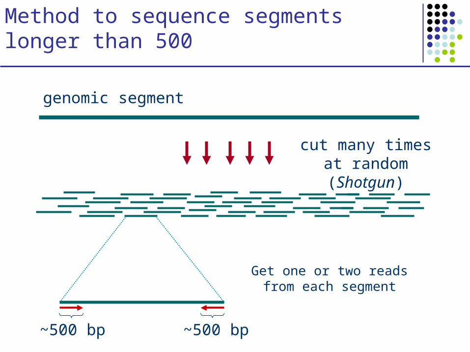
Method to sequence segments longer than 500

cut many times at random (Shotgun)

genomic segment

Get one or two reads from each segment

~500 bp ~500 bp

Reconstructing the Sequence (Fragment Assembly)

Cover region with ~7-fold redundancy (7X)

Overlap reads and extend to reconstruct the original genomic region

reads

Definition of Coverage

Length of genomic segment: LNumber of reads: nLength of each read: l

Definition: Coverage C = n l / L

How much coverage is enough?

Lander-Waterman model:Assuming uniform distribution of reads, C=10 results in 1 gapped region /1,000,000 nucleotides

C

Challenges with Fragment Assembly

• Sequencing errors

~1-2% of bases are wrong

• Repeats

• Computation: ~ O( N2 ) where N = # reads

false overlap due to repeat

Repeats

Bacterial genomes: 5%Mammals: 50%

Repeat types:

• Low-Complexity DNA (e.g. ATATATATACATA…)

• Microsatellite repeats (a1…ak)N where k ~ 3-6(e.g. CAGCAGTAGCAGCACCAG)

• Transposons SINE (Short Interspersed Nuclear Elements)

e.g., ALU: ~300-long, 106 copies LINE (Long Interspersed Nuclear Elements)

~500-5,000-long, 200,000 copies LTR retroposons (Long Terminal Repeats (~700 bp) at each end)

cousins of HIV

• Gene Families genes duplicate & then diverge (paralogs)

• Recent duplications ~100,000-long, very similar copies

Strategies for whole-genome sequencing

1. Hierarchical – Clone-by-clone yeast, worm, humani. Break genome into many long fragmentsii. Map each long fragment onto the genomeiii. Sequence each fragment with shotgun

2. Online version of (1) – Walking rice genomei. Break genome into many long fragmentsii. Start sequencing each fragment with shotguniii. Construct map as you go

3. Whole Genome Shotgun fly, human, mouse, rat, fugu

One large shotgun pass on the whole genome

Hierarchical Sequencing

Hierarchical Sequencing Strategy

1. Obtain a large collection of BAC clones2. Map them onto the genome (Physical Mapping)3. Select a minimum tiling path4. Sequence each clone in the path with shotgun5. Assemble6. Put everything together

a BAC clone

mapgenome

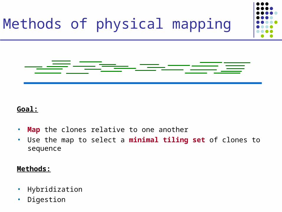
Methods of physical mapping

Goal:

• Map the clones relative to one another • Use the map to select a minimal tiling set of clones to sequence

Methods:

• Hybridization• Digestion

1. Hybridization

Short words, the probes, attach to complementary words

1. Construct many probes p1, p2, …, pn

2. Treat each clone Ci with all probes

3. Record all attachments (Ci, pj)

4. Same words attaching to clones X, Y overlap

p1 pn

Hybridization – Computational Challenge

Matrix:m probes n clones

(i, j): 1, if pi hybridizes to Cj

0, otherwise

Definition: Consecutive ones matrix1s are consecutive in each row & col

Computational problem:Reorder the probes so that matrix is in consecutive-ones form

Can be solved in O(m3) time (m > n)

p1 p2 …………………….pm

C1

C2 …

……

……

….C

n

1 0 1…………………...01 1 0 …………………..0

0 0 1 …………………..1

pi1pi2…………………….pim

Cj1C

j2 …

……

……

….C

jn

1 1 1 0 0 0……………..00 1 1 1 1 1……………..00 0 1 1 1 0……………..0

0 0 0 0 0 0………1 1 1 00 0 0 0 0 0………0 1 1 1

Hybridization – Computational Challenge

If we put the matrix in consecutive-ones form,

then we can deduce the order of the clones

& which pairs of clones overlap

pi1pi2…………………….pim

Cj1C

j2 …

……

……

….C

jn

1 1 1 0 0 0……………..00 1 1 1 1 1……………..00 0 1 1 1 0……………..0

0 0 0 0 0 0………1 1 1 00 0 0 0 0 0………0 1 1 1 C

j1C

j2 …

……

……

….C

jn

pi1pi2………………………………….pim

Hybridization – Computational Challenge

Additional challenge:

A probe (short word) can hybridize in many places in the genome

Computational Problem:

Find the order of probes that implies the minimal probe repetition

Equivalent: find the shortest string of probes such that each clone appears as a substring

APX-hard

Solutions:Greedy, Probabilistic, Lots of manual curation

p1 p2 …………………….pm

C1

C2 …

……

……

….C

n

1 0 1…………………...01 1 0 …………………..0

0 0 1 …………………..1

2. Digestion

Restriction enzymes cut DNA where specific words appear

1. Cut each clone separately with an enzyme2. Run fragments on a gel and measure length3. Clones Ca, Cb have fragments of length { li, lj, lk } overlap

Double digestion:Cut with enzyme A, enzyme B, then enzymes A + B

Online Clone-by-cloneThe Walking Method

The Walking Method

1. Build a very redundant library of BACs with sequenced clone-ends (cheap to build)

2. Sequence some seed clones

3. Walk from seeds using clone-ends to pick library clones that extend left & right

Walking: An Example

Advantages & Disadvantages of Hierarchical Sequencing

• Hierarchical Sequencing ADV. Easy assembly DIS. Build library & physical map; redundant sequencing

• Whole Genome Shotgun (WGS) ADV. No mapping, no redundant sequencing DIS. Difficult to assemble and resolve repeats

The Walking method – motivation

Sequence the genome clone-by-clone without a physical mapThe only costs involved are:

Library of end-sequenced clones (CHEAP) Sequencing

Walking off a Single Seed

• ADV: Low redundant sequencing

• DIS: Too many sequential steps

Walking off Several Seeds in Parallel

• Few sequential steps

• Additional redundant sequencing

In general, can sequence a genome in ~5 walking steps, with <20% redundant sequencing

Efficient Inefficient