conrob programming assignments manual coursera sp14 (1)

8/13/2019 Conrob Programming Assignments Manual Coursera Sp14 (1)

http://slidepdf.com/reader/full/conrob-programming-assignments-manual-coursera-sp14-1 1/9

Sim.I.am: A Robot SimulatorCoursera: Control of Mobile Robots

Jean-Pierre de la Croix

Last Updated: January 23, 2014

Contents

1 Introduction 21.1 Installation . . . . . . . . . . . . . . . . . . . . . . . . . . . . . . . . . . . . . . . . . . . . 21.2 Requirements . . . . . . . . . . . . . . . . . . . . . . . . . . . . . . . . . . . . . . . . . . . 21.3 Bug Reporting . . . . . . . . . . . . . . . . . . . . . . . . . . . . . . . . . . . . . . . . . . 2

2 Mobile Robot 32.1 IR Range Sensors . . . . . . . . . . . . . . . . . . . . . . . . . . . . . . . . . . . . . . . . . 32.2 Differential Wheel Drive . . . . . . . . . . . . . . . . . . . . . . . . . . . . . . . . . . . . . 42.3 Wheel Encoders . . . . . . . . . . . . . . . . . . . . . . . . . . . . . . . . . . . . . . . . . . 5

3 Simulator 6

4 Programming Assignments 74.1 Week 1 . . . . . . . . . . . . . . . . . . . . . . . . . . . . . . . . . . . . . . . . . . . . . . . 74.2 Week 2 . . . . . . . . . . . . . . . . . . . . . . . . . . . . . . . . . . . . . . . . . . . . . . . 7

1



1 Introduction

This manual is going to be your resource for using the simulator with the programming assignmentsfeatured in the Coursera course, Control of Mobile Robots (and included at the end of this manual). Itwill be updated from time to time whenever new features are added to the simulator or any correctionsto the course material are made.

1.1 Installation

Download simiam-coursera-week-X.zip (where X is the corresponding week number for the assignment)from the course page on Coursera under Programming Assignments . Make sure to download a new copyof the simulator before you start a new week’s programming assignment, or whenever an announcementis made that a new version is available. It is important to stay up-to-date, since new versions may containimportant bug xes or features required for the programming assignment.

Unzip the .zip le to any directory.

1.2 Requirements

You will need a reasonably modern computer to run the robot simulator. While the simulator will runon hardware older than a Pentium 4, it will probably be a very slow experience. You will also need acopy of MATLAB.

Thanks to support from MathWorks, a license for MATLAB and all required toolboxes is availableto all students for the duration of the course. Check the Getting Started with MATLAB section underProgramming Assignments on the course page for detailed instructions on how to download and installMATLAB on your computer.

1.3 Bug Reporting

If you run into a bug (issue) with the simulator, please create a post on the discussion forums in theProgramming Assignments section. Make sure to leave a detailed description of the bug. Any questionsor issues with MATLAB itself should be posted on the discussion forums in the MATLAB section.

2

https://class.coursera.org/conrob-002/wiki/ProgrammingAssignments



https://class.coursera.org/conrob-002/forum/list?forum_id=3








(a) Simulated QuickBot (b) Actual QuickBot

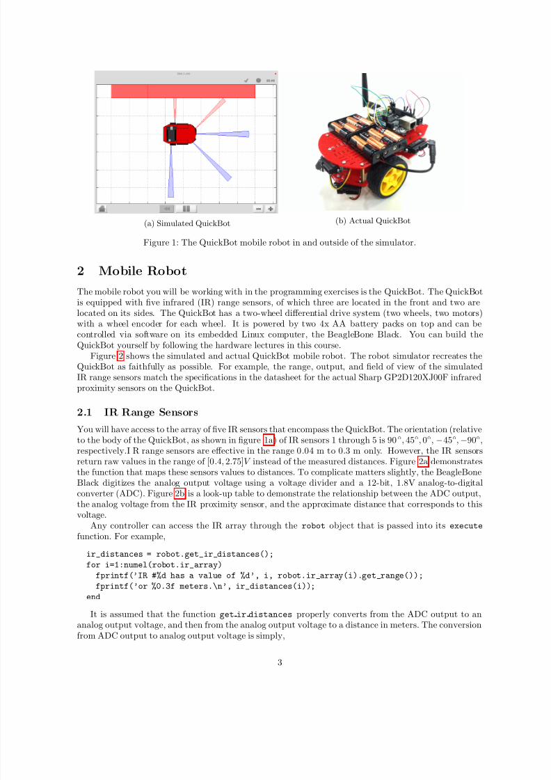
Figure 1: The QuickBot mobile robot in and outside of the simulator.

2 Mobile RobotThe mobile robot you will be working with in the programming exercises is the QuickBot. The QuickBotis equipped with ve infrared (IR) range sensors, of which three are located in the front and two arelocated on its sides. The QuickBot has a two-wheel differential drive system (two wheels, two motors)with a wheel encoder for each wheel. It is powered by two 4x AA battery packs on top and can becontrolled via software on its embedded Linux computer, the BeagleBone Black. You can build theQuickBot yourself by following the hardware lectures in this course.

Figure 2 shows the simulated and actual QuickBot mobile robot. The robot simulator recreates theQuickBot as faithfully as possible. For example, the range, output, and eld of view of the simulatedIR range sensors match the specications in the datasheet for the actual Sharp GP2D120XJ00F infraredproximity sensors on the QuickBot.

2.1 IR Range SensorsYou will have access to the array of ve IR sensors that encompass the QuickBot. The orientation (relativeto the body of the QuickBot, as shown in gure 1a) of IR sensors 1 through 5 is 90 ◦ , 45◦ , 0◦ , − 45◦ , − 90◦ ,respectively.I R range sensors are effective in the range 0 .04 m to 0.3 m only. However, the IR sensorsreturn raw values in the range of [0 .4, 2.75]V instead of the measured distances. Figure 2a demonstratesthe function that maps these sensors values to distances. To complicate matters slightly, the BeagleBoneBlack digitizes the analog output voltage using a voltage divider and a 12-bit, 1.8V analog-to-digitalconverter (ADC). Figure 2b is a look-up table to demonstrate the relationship between the ADC output,the analog voltage from the IR proximity sensor, and the approximate distance that corresponds to thisvoltage.

Any controller can access the IR array through the robot object that is passed into its executefunction. For example,

ir_distances = robot.get_ir_distances();for i=1:numel(robot.ir_array)

fprintf(’IR #%d has a value of %d’, i, robot.ir_array(i).get_range());fprintf(’or %0.3f meters.\n’, ir_distances(i));

end

It is assumed that the function get ir distances properly converts from the ADC output to ananalog output voltage, and then from the analog output voltage to a distance in meters. The conversionfrom ADC output to analog output voltage is simply,

3



0 0.05 0.1 0.15 0.2 0.25 0.3 0.350

0.5

1

1.5

2

2.5

3

Distance (m)

V o

l t a g e

( V )

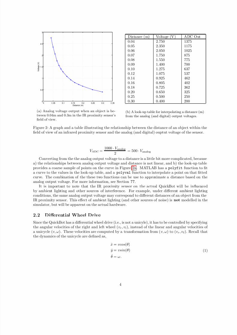
(a) Analog voltage output when an object is be-tween 0.04m and 0.3m in the IR proximity sensor’seld of view.

Distance (m) Voltage (V) ADC Out0.04 2.750 13750.05 2.350 11750.06 2.050 10250.07 1.750 8750.08 1.550 7750.09 1.400 7000.10 1.275 6370.12 1.075 5370.14 0.925 4620.16 0.805 4020.18 0.725 3620.20 0.650 3250.25 0.500 2500.30 0.400 200

(b) A look-up table for interpolating a distance (m)

from the analog (and digital) output voltages.

Figure 2: A graph and a table illustrating the relationship between the distance of an object within theeld of view of an infrared proximity sensor and the analog (and digital) ouptut voltage of the sensor.

V ADC = 1000 · V analog

2 = 500 · V analog

Converting from the the analog output voltage to a distance is a little bit more complicated, becausea) the relationships between analog output voltage and distance is not linear, and b) the look-up tableprovides a coarse sample of points on the curve in Figure 2a. MATLAB has a polyfit function to ta curve to the values in the look-up table, and a polyval function to interpolate a point on that ttedcurve. The combination of the these two functions can be use to approximate a distance based on theanalog output voltage. For more information, see Section ?? .

It is important to note that the IR proximity sensor on the actual QuickBot will be inuencedby ambient lighting and other sources of interference. For example, under different ambient lightingconditions, the same analog output voltage may correspond to different distances of an object from theIR proximity sensor. This effect of ambient lighting (and other sources of noise) is not modelled in thesimulator, but will be apparent on the actual hardware.

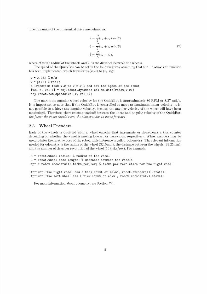
2.2 Differential Wheel Drive

Since the QuickBot has a differential wheel drive (i.e., is not a unicyle), it has to be controlled by specifyingthe angular velocities of the right and left wheel ( vr , v l ), instead of the linear and angular velocities of a unicycle ( v, ω ). These velocities are computed by a transformation from ( v, ω ) to ( vr , v ). Recall thatthe dynamics of the unicycle are dened as,

x = vcos (θ)y = vsin (θ)

θ = ω.

(1)

4



3 Simulator

Start the simulator with the launch command in MATLAB from the command window. It is importantthat this command is executed inside the unzipped folder (but not inside any of its subdirectories).

(a) Simulator (b) Submission screen

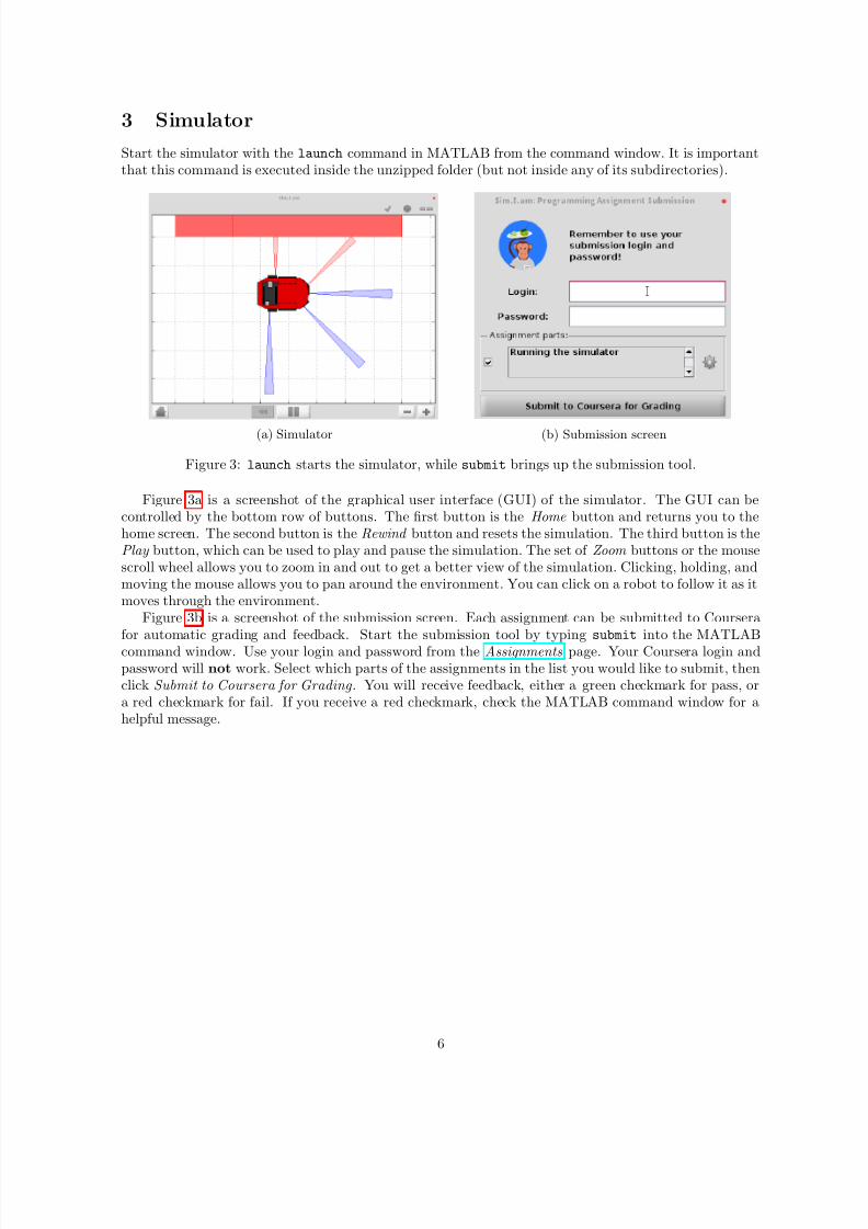
Figure 3: launch starts the simulator, while submit brings up the submission tool.

Figure 3a is a screenshot of the graphical user interface (GUI) of the simulator. The GUI can becontrolled by the bottom row of buttons. The rst button is the Home button and returns you to thehome screen. The second button is the Rewind button and resets the simulation. The third button is thePlay button, which can be used to play and pause the simulation. The set of Zoom buttons or the mousescroll wheel allows you to zoom in and out to get a better view of the simulation. Clicking, holding, andmoving the mouse allows you to pan around the environment. You can click on a robot to follow it as itmoves through the environment.

Figure 3b is a screenshot of the submission screen. Each assignment can be submitted to Courserafor automatic grading and feedback. Start the submission tool by typing submit into the MATLABcommand window. Use your login and password from the Assignments page. Your Coursera login andpassword will not work. Select which parts of the assignments in the list you would like to submit, thenclick Submit to Coursera for Grading . You will receive feedback, either a green checkmark for pass, ora red checkmark for fail. If you receive a red checkmark, check the MATLAB command window for ahelpful message.

6

https://class.coursera.org/conrob-002/assignment/list

https://class.coursera.org/conrob-002/assignment/list



4 Programming Assignments

The following sections serve as a tutorial for getting through the simulator portions of the programmingexercises. Places where you need to either edit or add code is marked off by a set of comments. Forexample,

%% START CODE BLOCK %%[edit or add code here]

%% END CODE BLOCK %%

To start the simulator with the launch command from the command window, it is important thatthis command is executed inside the unzipped folder (but not inside any of its subdirectories).

4.1 Week 1

This week’s exercises will help you learn about MATLAB and robot simulator:

1. Since the assignments in this course involve programming in MATLAB, you should familiarizeyourself with MATLAB (both the environment and the language). Review the resources posted in

the ”Getting Started with MATLAB” section on the Programming Assignments page.2. Familiarize yourself with the simulator by reading this manual and downloading the robot simulator

posted on the Programming Assignments section on the Coursera page.

4.2 Week 2

Start by downloading the robot simulator for this week from the Week 2 programming assignment. Beforeyou can design and test controllers in the simulator, you will need to implement three components of thesimulator:

1. Implement the transformation from unicycle dynamics to differential drive dynamics, i.e. convertfrom (v, ω ) to the right and left angular wheel speeds (vr , v l ).

In the simulator, ( v, ω ) corresponds to the variables v and w, while (vr , v l ) correspond to thevariables vel r and vel l . The function used by the controllers to convert from unicycle dynamicsto differential drive dynamics is located in +simiam/+robot/+dynamics/DifferentialDrive.m .The function is named uni to diff , and inside of this function you will need to dene vel r (vr )and vel l (vl ) in terms of v, w, R, and L. R is the radius of a wheel, and L is the distance separatingthe two wheels. Make sure to refer to Section 2.2 on “Differential Wheel Drive” for the dynamics.

2. Implement odometry for the robot, such that as the robot moves around, its pose ( x,y,θ ) is esti-mated based on how far each of the wheels have turned. Assume that the robot starts at (0,0,0).The tutorial located at www.orcboard.org/wiki/images/1/1c/OdometryTutorial.pdf covers howodometry is computed. The general idea behind odometry is to use wheel encoders to measure thedistance the wheels have turned over a small period of time, and use this information to approximatethe change in pose of the robot.The pose of the robot is composed of its position ( x, y ) and its orientation θ on a 2 dimensionalplane ( note : the video lecture may refer to robot’s orientation as φ). The currently estimatedpose is stored in the variable state estimate , which bundles x (x ), y (y), and theta (θ). Therobot updates the estimate of its pose by calling the update odometry function, which is locatedin +simiam/+controller/+quickbot/QBSupervisor.m . This function is called every dt seconds,where dt is 0.033s (or a little more if the simulation is running slower).

7



https://github.com/jdelacroix/simiam/tags

http://www.orcboard.org/wiki/images/1/1c/OdometryTutorial.pdf

http://www.orcboard.org/wiki/images/1/1c/OdometryTutorial.pdf

https://github.com/jdelacroix/simiam/tags





% Get wheel encoder ticks from the robotright_ticks = obj.robot.encoders(1).ticks;left_ticks = obj.robot.encoders(2).ticks;

% Recall the wheel encoder ticks from the last estimateprev_right_ticks = obj.prev_ticks.right;prev_left_ticks = obj.prev_ticks.left;

% Previous estimate[x, y, theta] = obj.state_estimate.unpack();

% Compute odometry hereR = obj.robot.wheel_radius;L = obj.robot.wheel_base_length; m_per_tick = (2*pi*R)/obj.robot.encoders(1).ticks_per_rev;

The above code is already provided so that you have all of the information needed to estimate thechange in pose of the robot. right ticks and left ticks are the accumulated wheel encoder ticks

of the right and left wheel. prev right ticks and prev left ticks are the wheel encoder ticksof the right and left wheel saved during the last call to update odometry . R is the radius of eachwheel, and L is the distance separating the two wheels. m per tick is a constant that tells youhow many meters a wheel covers with each tick of the wheel encoder. So, if you were to multiply m per tick by (right ticks -prev right ticks ), you would get the distance travelled by the rightwheel since the last estimate.Once you have computed the change in ( x,y,θ ) (let us denote the changes as x dt , y dt , andtheta dt ) , you need to update the estimate of the pose:

theta_new = theta + theta_d;x_new = x + x_dt;y_new = y + y_dt;

3. Read the ”IR Range Sensors” section in the manual and take note of the table in Figure 2b, whichmaps distances (in meters) to raw IR values. Implement code that converts raw IR values todistances (in meters).To retrieve the distances (in meters) measured by the IR proximity sensor, you will need to imple-ment a conversion from the raw IR values to distances in the get ir distances function locatedin +simiam/+robot/Quickbot.m .

function ir_distances = get_ir_distances(obj)ir_array_values = obj.ir_array.get_range();ir_voltages = ir_array_values;coeff = [];ir_distances = polyval(coeff, ir_voltages);

end

The variable ir array values is an array of the IR raw values. Divide this array by 500 to computethe ir voltages array. The coeff should be the coefficients returned by

coeff = polyfit(ir_voltages_from_table, ir_distances_from_table, 5);

where the rst input argument is an array of IR voltages from the table in Figure 2b and the secondargument is an array of the corresponding distances from the table in Figure 2b. The third argumentspecies that we will use a fth-order polynomial to t to the data. Instead of running this t every

8



time, execute the polyt once in the MATLAB command line, and enter them manually on thethird line, i.e. coeff = [ ... ]; . If the coefficients are properly computed, then the last linewill use polyval to convert from IR voltages to distances using a fth-order polynomial using thecoefficients in coeff .

How to test it allTo test your code, the simulator will is set to run a single P-regulator that will steer the robot to a partic-ular angle (denoted θd or, in code, theta d ). This P-regulator is implemented in +simiam/+controller/GoToAngle.m . If you want to change the linear velocity of the robot, or the angle to which it steers, editthe following two lines in +simiam/+controller/+quickbot/QBSupervisor.m

obj.theta_d = pi/4;obj.v = 0.1; %m/s

1. To test the transformation from unicycle to differential drive, rst set obj.theta d=0 . The robotshould drive straight forward. Now, set obj.theta d to positive or negative π

4 . If positive, the robotshould start off by turning to its left, if negative it should start off by turning to its right. Note :If you haven’t implemented odometry yet, the robot will just keep on turning in that direction.

2. To test the odometry, rst make sure that the transformation from unicycle to differential driveworks correctly. If so, set obj.theta d to some value, for example π

4 , and the robot’s P-regulatorshould steer the robot to that angle. You may also want to uncomment the fprintf statement inthe update odometry function to print out the current estimate position to see if it make sense.Remember, the robot starts at ( x,y,θ ) = (0 , 0, 0).

3. To test the IR raw to distances conversion, edit +simiam/+controller/GoToAngle.m and uncom-ment the following section:

% for i=1:numel(ir_distances)% fprintf(’IR %d: %0.3fm\n’, i, ir_distances(i));% end

This for loop will print out the IR distances. If there are no obstacles (for example, walls) aroundthe robot, these values should be close (if not equal to) 0 .3m. Once the robot gets within range of a wall, these values should decrease for some of the IR sensors (depending on which ones can sensethe obstacle). Note: The robot will eventually collide with the wall, because we have not designedan obstacle avoidance controller yet!

9

conrob programming assignments manual coursera sp14 (1)

Documents