consequences of loan-to-value ratio policies for business
TRANSCRIPT

Consequences of Loan-to-Value Ratio Policies forBusiness and Credit Cycles
Tim Robinson Fang Yao1
University of Melbourne RBNZ
Sept 2016
1The views expressed here are those of the authors and do not necessarily re�ect the positionof the Reserve Bank of New Zealand.
Motivation I
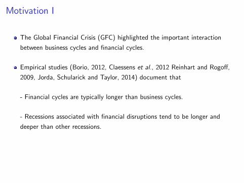
The Global Financial Crisis (GFC) highlighted the important interaction
between business cycles and �nancial cycles.
Empirical studies (Borio, 2012, Claessens et al., 2012 Reinhart and Rogo¤,
2009, Jorda, Schularick and Taylor, 2014) document that
- Financial cycles are typically longer than business cycles.
- Recessions associated with �nancial disruptions tend to be longer and
deeper than other recessions.
There has been increased usage of macroprudential policies in many
countries, with the aim of promoting �nancial stability.
Motivation I
The Global Financial Crisis (GFC) highlighted the important interaction
between business cycles and �nancial cycles.
Empirical studies (Borio, 2012, Claessens et al., 2012 Reinhart and Rogo¤,
2009, Jorda, Schularick and Taylor, 2014) document that
- Financial cycles are typically longer than business cycles.
- Recessions associated with �nancial disruptions tend to be longer and
deeper than other recessions.
There has been increased usage of macroprudential policies in many
countries, with the aim of promoting �nancial stability.
Question
What are the consequences of macroprudential policy in terms ofcyclical behaviors of business and credit cycles?

Literature
A large volume of DSGE literature are being developed to evaluate
macroprudential policies in terms of social welfare.
e.g. Monecelli (2006), Rubio (2009), Quint and Rabanal (2013), Lambertini
et al. (2013), Alpanda and Zubairy (2014)...
An emerging literature uses business-cycle dating methods (Bry and Boschan,
1971) to examine economic cycles and studies the e¤ects of macro policies
on those cycles.
- Albuquerue et al. (2015), Blanchard et al. (2015), Pagan and Robinson
(2014)
This approach allows researchers to examine cyclical consequences of
macroprudential policy in the lights of empirical evidence that motivated
those policies.
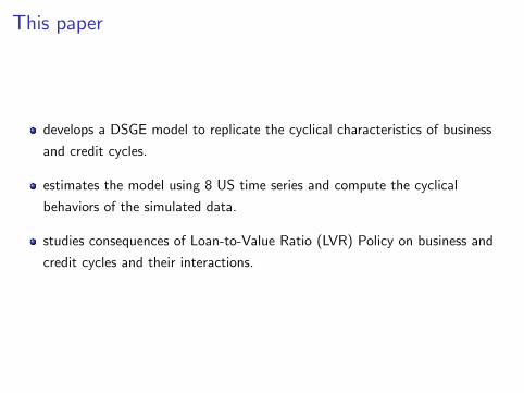
This paper
develops a DSGE model to replicate the cyclical characteristics of business
and credit cycles.
estimates the model using 8 US time series and compute the cyclical
behaviors of the simulated data.
studies consequences of Loan-to-Value Ratio (LVR) Policy on business and
credit cycles and their interactions.

Preview of results
The LVR policy rules face the trade-o¤ between the ampli�cation and
frequency of recessions.
We �nd that a LVR rule responding to house prices generates the best
trade-o¤ among rules investigated.
Credit-to-GDP ratio is not a good indicator of LVR policy, because credit is a
slow-moving variable relative to GDP.

Cyclical Characteristics
Empirical Approach
By the cycle we mean the classical cycle - �uctuations in the level of
economic activity.
Harding and Pagan (2002) develop an algorithm, drawing on Bry and
Boschan (1971), that identi�es turning points in the level of GDP.
By focusing on turning points it is not necessary to extract the low frequency
components (such as HP �lter).

US Cycles
Year1960 1970 1980 1990 2000 2010
Log
leve
l
3.8
3.6
3.4
3.2
3
2.8
2.6Real GDP
Year1960 1970 1980 1990 2000 2010
11
10.5
10
9.5
9
8.5
8
7.5
7Real Mortgage Debt
Data source: Federal Reserve of St Louis database

Cyclical Characteristics
Recession Our Data Claessens et al. (2012)*Output Credit Output Credit**
Duration 6.28 9.66 3.88 5.39Amplitude -3.59% -5.62% -2.17% -4.38%
Note: * Claessens�s data: 21 OECD countries, 23 EM countries from 1960:1 - 2010:4.
** Credit: aggregate claims on the private sector by deposit money banks.

US Cycles
Year1960 1970 1980 1990 2000 2010
Log
leve
l
3.8
3.6
3.4
3.2
3
2.8
2.6Real GDP
Year1960 1970 1980 1990 2000 2010
11
10.5
10
9.5
9
8.5
8
7.5
7Real Mortgage Debt

Conditional Cyclical Characteristics
Recessionswith credit downturn without credit downturn
Duration 8.5 3.33Amplitude -4.96% -1.77%

The Model

The Model
Medium scale DSGE model with a housing collateral constraint, drawing on
Iacoviello and Neri (2010).
Two groups of household:I Patient - saversI Impatient - borrowers, subject to a collateral constraint.
Mortgage loansI Long-term mortgage loan (Garriga, Kydland and Sustek, 2013)
I Fixed mortgage rates (Alpanda and Zubairy, 2014)
Labour augmenting technology follows a unit root with drift.
Monetary policy is set via a Taylor rule.
Permanent LVR changes and countercyclical rules
Parameterization

Parameterization
We use 8 observed series from 1984:Q1 �2007:Q4.
- output growth - business investment growth- consumption growth - residential investment growth- federal Funds rate - in�ation- real wage growth - mortgage loan growth
Calibrated parameters
Parameter Value Ratio Data Modelβ, β0 0.993, 0.985 D
Y 1.40 1.58ξh , ξ
0h 0.14, 0.14 C
Y 0.637 0.622δh,δk 0.01, 0.013 I
Y 0.125 0.123ηk , ηl 0.17, 0.4 X
Y 0.047 0.063ηh , ηw 7.6, 7.6 K
Y 7.06 6.95m 0.9 H
Y 4.28 4.33Notes: Average over 1984:Q1 - 2007:4.
Parameterization
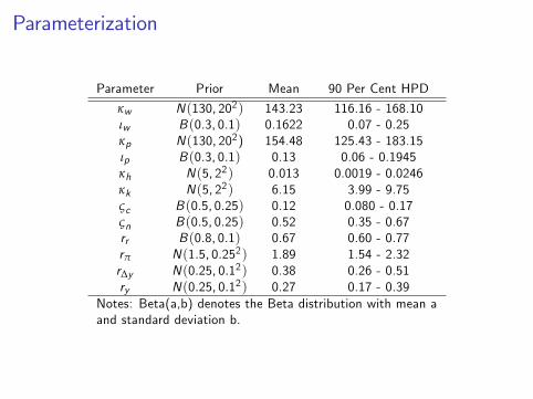
Parameter Prior Mean 90 Per Cent HPD
κw N(130, 202) 143.23 116.16 - 168.10ιw B(0.3, 0.1) 0.1622 0.07 - 0.25κp N(130, 202) 154.48 125.43 - 183.15ιp B(0.3, 0.1) 0.13 0.06 - 0.1945κh N(5, 22) 0.013 0.0019 - 0.0246κk N(5, 22) 6.15 3.99 - 9.75ςc B(0.5, 0.25) 0.12 0.080 - 0.17ςn B(0.5, 0.25) 0.52 0.35 - 0.67rr B(0.8, 0.1) 0.67 0.60 - 0.77rπ N(1.5, 0.252) 1.89 1.54 - 2.32r∆y N(0.25, 0.12) 0.38 0.26 - 0.51ry N(0.25, 0.12) 0.27 0.17 - 0.39
Notes: Beta(a,b) denotes the Beta distribution with mean aand standard deviation b.

Parameterization
Parameter Description Prior Mean 90 per cent HPD
ρm Monetary B (0.5, 0.15) 0.64 0.50 - 0.78ρp Prices Cost-push B (0.5, 0.15) 0.65 0.42 - 0.83ρc Preferences B (0.5, 0.15) 0.88 0.85 - 0.92ρhd Housing Demand B (0.5, 0.15) 0.13 0.04 - 0.23ρah Housing Technology B (0.5, 0.15) 0.89 0.84 - 0.94ρak Investment Technology B (0.5, 0.15) 0.75 0.66 - 0.85ρg Fiscal B (0.5, 0.15) 0.98 0.97 - 0.99ρw Wages cost-push B (0.5, 0.15) 0.19 0.09 - 0.29ρz Technology B (0.5, 0.15) 0.79 0.75 - 0.83σm Monetary IG(0.1,0.5) 0.16 0.13 - 0.20σp Cost-push IG(1,1.5) 2.80 1.62 - 3.94σc Preferences IG(1,1.5) 2.43 2.0 - 2.8σhd Housing Demand IG(1,1.5) 28.19 20.6 - 37.19σah Housing Technology IG(1,1.5) 2.8 1.95 - 3.46σak Investment Technology IG(1,1.5) 33.1 19.6 - 48.7σg Fiscal IG(1,1.5) 1.6 1.45 - 1.96σz Technology IG(1,1.5) 0.18 0.15 - 0.21σw Wages Cost-push IG(1,1.5) 15.9 12.06 - 19.37
Notes: IG the Inverse Gamma distribution. The arguments arethe mean andstandard deviation.

Applying BBQ to the DSGE model
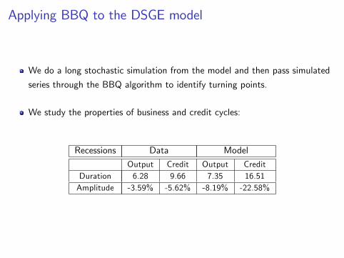
We do a long stochastic simulation from the model and then pass simulated
series through the BBQ algorithm to identify turning points.
We study the properties of business and credit cycles:
Applying BBQ to the DSGE model
We do a long stochastic simulation from the model and then pass simulated
series through the BBQ algorithm to identify turning points.
We study the properties of business and credit cycles:
Recessions Data ModelOutput Credit Output Credit
Duration 6.28 9.66 7.35 16.51Amplitude -3.59% -5.62% -8.19% -22.58%
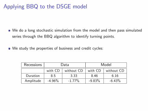
Applying BBQ to the DSGE model
We do a long stochastic simulation from the model and then pass simulated
series through the BBQ algorithm to identify turning points.
We study the properties of business and credit cycles:
Recessions Data Modelwith CD without CD with CD without CD
Duration 8.5 3.33 8.46 6.16Amplitude -4.96% -1.77% -9.83% -6.43%

E¤ects of LVR on Cycles
Policy Analysis
We consider both permanent changes in LVR and countercyclical LVR
response rules.
The permanent LVR rule is a one-o¤ change in the steady state level of LVR
in the economy.
For the countercyclical LVR rule, we model the absolute deviation of the LTV
from its steady-state, m̂t , as:
m̂t = ηLVR f̃t ,
where ηLVR is a negative coe¢ cient governing the reaction to the variable f̃t :
I house price
I credit-to-GDP ratio

Permanent LVR Changes
Normal v.s. Financial-downturn recessions
Loantovalue Ratio0.4 0.5 0.6 0.7 0.8
Qua
rter
5.5
6
6.5
7
7.5
8
8.5
9Duration
Loantovalue Ratio0.4 0.5 0.6 0.7 0.8
%
6
7
8
9
10
11
12Amplitude
With credit downturn Without credit downturn
Loantovalue Ratio0.4 0.5 0.6 0.7 0.8
%
17
17.5
18
18.5
19
19.5
20Frequency

Countercyclical LVR rule - Credit-to-GDP ratioNormal v.s. Financial-downturn recessions
LVR
5 4 3 2 1 0
Qua
rter
5
5.5
6
6.5
7
7.5
8
8.5
9Duration
LVR
5 4 3 2 1 0
%
6
8
10
12
14
16
18
20Amplitude
With credit downturn Without credit downturn
LVR
5 4 3 2 1 0%
17
17.5
18
18.5
19
19.5
20
20.5
21
21.5
22Frequency
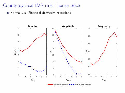
Countercyclical LVR rule - house priceNormal v.s. Financial-downturn recessions
LVR
5 4 3 2 1 0
Qua
rter
5.5
6
6.5
7
7.5
8
8.5
9Duration
LVR
5 4 3 2 1 0
%
6
8
10
12
14
16
18
20Amplitude
With credit downturn Without credit downturn
LVR
5 4 3 2 1 0
%
14
15
16
17
18
19
20Frequency

LVR Policy Trade-o¤s
Normal recessions Financial-downturn recessionsDuration Amplitude Duration Amplitude Frequency
Permanent LVR no no no up downLVR_Credit-GDP down up no up upLVR_House price no up down up down
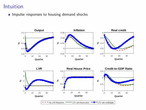
IntuitionImpulse responses to housing demand shocks
Quarter0 10 20 30
%
0.6
0.4
0.2
0
0.2Output
No LVR Response LTV rulehouse price LTV rulecredit2gdp
Quarter0 10 20 30%
0.02
0
0.02
0.04
0.06Inflation
Quarter0 10 20 30
%
0.8
0.6
0.4
0.2
0Real credit
Quarter0 10 20 30
%
1
0
1
2
3LVR
Quarter0 10 20 30
%
1
0.5
0
0.5Real House Price
Quarter0 10 20 30
%
1
0.5
0
0.5CredittoGDP Ratio
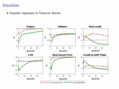
Intuition
Impulse responses to �nancial shocks
Quarter0 10 20 30
%
3
2
1
0Output
LTV rulehouse price LTV rulecredit2gdp
Quarter0 10 20 30
%1
0.5
0
0.5Inflation
Quarter0 10 20 30
%
2
0
2
4Real credit
Quarter0 10 20 30
%
30
20
10
0
10LVR
Quarter0 10 20 30
%
3
2
1
0Real House Price
Quarter0 10 20 30
%
5
0
5
10CredittoGDP Ratio

Conclusion
We use business cycle dating methods to examine what are the
macroeconomic e¤ects of LVR policies.
The LVR policy rules face the trade-o¤ between the ampli�cation and
frequency of recessions.
LVR rule responding to house prices generates the best trade-o¤ among
indicator variables investigated.
Credit-to-GDP ratio is not a good indicator of LVR policy, because credit is a
slow-moving variable relative to GDP.
Figure Appendix
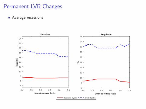
Permanent LVR Changes
Average recessions
Loantovalue Ratio0.4 0.5 0.6 0.7 0.8 0.9
Qua
rter
4
6
8
10
12
14
16
18
20
22
24
Duration
Business Cycles Credit Cycles
Loantovalue Ratio0.4 0.5 0.6 0.7 0.8 0.9
%
6
8
10
12
14
16
18
20
22
24
26Amplitude

Countercyclical LVR rule - credit-to-GDPAverage recessions
LVR
5 4 3 2 1 0
Qua
rter
4
6
8
10
12
14
16
18
20
22
24Duration
LVR
5 4 3 2 1 0
%
6
8
10
12
14
16
18
20
22
24
26Amplitude
Business Cycles Credit Cycles
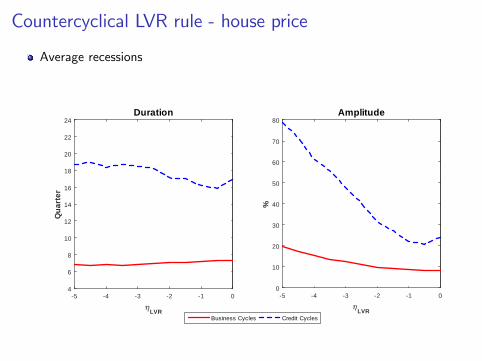
Countercyclical LVR rule - house price
Average recessions
LVR
5 4 3 2 1 0
Qua
rter
4
6
8
10
12
14
16
18
20
22
24Duration
LVR
5 4 3 2 1 0
%
0
10
20
30
40
50
60
70
80Amplitude
Business Cycles Credit Cycles