conservation laws. the method of and solution element
TRANSCRIPT

NASA Technical Memorandum 104495
A New Numerical Framework for SolvingConservation_Laws. The Method of__
..........................
Space-Time ConservationE!ementand Solution Element
Sin-Chung Chang
National Aeronautics and Space AdministrationLewis _Research Center .......
Cleveland, Ohio
and
Wai-Ming To
Sverdrup Technology, Inc. :- _: _ : " : _ : :L
Lewis Research Center GroupBrook Park, Ohio
August 1991
(_ASA-T_-1044QS) A NFW NUIq[RICAL FRAMEWORK Nqi-3086/
FOR _nLVING Cn,WSERVATIi]N LAW3,: THE METHOD OF
SPACE-TIM_ CCJNSf-RVATION _!LEMENT AND SOLUTION ,.-i_ -
....ELEMENT (NASA) ]15 p CSCL 12A Unc|as :-G3/_4_ 0037'_5
NASA

T|!
SUMMARY
A new numerical framework for solving conservation laws is being developed. This new
approach differs substantially from the well established methods, i.e., finite difference, finite
volume, finite element, and spectral methods, in both concept and methodology. It employs:
a. a nontraditional formulation of the conservation laws in which space and time am unified
and treated on the same footing; and
b. a nontraditional use of discrete variables such that numerical marching can be carded out
by using a set of relations that represents both local and global flux conservation.
To be specific, we consider a conservation law that governs the convection and diffusion of a
physical variable in a 1-D space. Let (i) x be the spatial coordinate, (ii) Co > 0 be a conversion
constant with the dimension of velocity, and (iii) t be the product of Co and the temporal
coordinate. By definition, x and t have the same dimension. As a result, xl = x and Xz = t may be
considered as the coordinates of a two-dimensional Euclidean space E2 (also referred to as a
space-time). Let u(x,t) be a scalar function ofx and t. Let a be a dimensionless constant and Ix
(> 0) be a constant with the dimension of length. Then the conservation law may be expressed
as
scv = o (o.1)
where (i) S(V) is the boundary of an arbitrary volume V in E2, (ii)
_u-_ d_e_f( au _ lX.__x , U ) (0.2)
is a current density vector in E 2, and (iii) _ = do, with dc_ and _, respectively, being the area
and the outward unit normal of a surface element on S (V). By applying the divergence theorem
in E2, Eq. (0.1) implies the unsteady convection-diffusion equation, i.e.,
_u _u _2u
3---T+ a _ - IX_ = 0 (0.3)
Let E z be divided into nonoverlapping regions referred to as conservation elements (see Figs.
2.1(a) and 2.1(b)). A conservation element and its interior, respectively, may be denoted by
CE(j,n) and CE"(j,n) where j and n, respectively, are the spatial and temporal indices. For
(x,t) _ CE"(j',n), u(x,t) will be approximated by
u(x,t) d_J _'_(x-x]) + _](t-t") + 7_ (0.4)
where ot_, _ and _ are constants in CE"(j,n), and (x_,t") are the coordinates of the center of
-1-

CE(j,n). For(x,t)e CE"(j,n),h (x,t) will be approximated by
3u (x, t)h(x,t) _ (au(x,t)- _t bx , _(x,t)) (0.5)
Furthermore, the conservation law Eq. (0. I) will be approximated by
0 (0.6)
where V is the union of any combination of conservation elements. Since _is not defined on
S (V), the above surface integration, by definition, is to be carried out over a surface which is in
the interior of V and immediately adjacent to S (V).
Because _ (x,t) and _(x,t) are continuous in the interior of a conservation element but may be
discontinuous across an interface separating two neighboring conservation elements, a
conservation element is also a solution element in the current scheme. As will be shown,
generally a conservation element is not necessarily a solution element and vice versa.
Let V = CE(j,n). Then Eqs. (0.4) - (0.6) and the divergence theorem imply that _7 = -a ct_.
As a result, Eq. (0.4) can be simplified as
u_.(x,t) = ctT[(x-xT)-a(t-tn)] + y_ , (x,t) _ CE"(j,n) (0.7)
Thus, for (x,t) e CE"(j,n), u (x,t) is determined by the parameters y_ and o_7. As will be shown,
by repeatedly applying Eq. (0.6) with V being the union of two neighboring conservation
elements, any pair of _ and o_)' can be determined in terms of _ and o_°, j = 0, +1, _-t:2, .-.. The
values of_j and tx°, in turn, can be determined by the initial condition.
Because
u__(x_,t") = y_ (0.8)
and
Ox - txj (x,t) _ CE (j,n) (0.9)
and etT, respectively, may be considered as the numerical counterparts of u(xT,t _) and
ux(x_,tn). In other words, both u and its spatial derivative at (xT,t n) are computed by the currentscheme.
In the current paper, we also
a° explore the concept of a dynamic space-time mesh (the conservation elements are
embedded in this mesh) and the need for a unified treatment of physical variables and mesh
parameters;
-2-
HII I-

b°
Co
study the stability, dissipation and dispersion of the current scheme by using a rigorous
Fourier analysis;
develop a new error analysis technique that enables us to predict and interpret the
numerical errors of the current and other classical schemes;
d. study the consistency and truncation error of the current scheme; and
e. compare the errors of the numerical solutions generated by the current scheme and other
classical schemes.
The key results obtained from the above study are:
a. It is demonstrated that (i) stability and accuracy can be improved, and (ii) dissipation and
dispersion can be reduced, if the space-time mesh is allowed to evolve with the physical
variable such that the local convective motion of physical variables relative to the moving
mesh is kept to a minimum. Because the appearance of wiggles near a discontinuity is a
result of numerical dispersion, these wiggles can also be reduced by reducing this relative
convective motion.
bo
C.
It is shown that there is a remarkable similarity between the forms of the amplification
factors of the Leapfrog/DuFort-Frankel and the current schemes. As a result of this
similarity, the stability condition of the current scheme, as in the case of the
Leapfrog/DuFort-Frankel scheme, is essentially the CFL condition and thus independent of
the viscosity _t. Therefore, the current scheme is unconditionally stable in the case of pure
diffusion. Also, as in the case of the Leapfrog/DuFort-Frankel scheme, the current scheme
has no numerical diffusion in the absence of viscosity. Note that the stability condition of a
classical explicit scheme for solving Eq. (0.3), e.g., the MacCormack scheme, generally is
more restrictive than the CFL condition. In the case where the mesh Reynolds number ,_
1, the stability bound for the time-step size At is more or less proportional to (Ax) 2. In
contrast, the same bound will still he determined by the CFL condition and therefore is
proportional to Ax if the current scheme is used. The advantage of the current scheme in
the allowable time-step size grows as Ax -_ O. This advantage becomes particularly
important when the current scheme is used in a steady-state calculation.
It is shown theoretically that the current scheme is more accurate than the
Leapfrog/DuFort-Frankel scheme by one order (in a sense to be defined in the paper) in
both initial-value specification and the marching scheme. It is also shown theoretically that
the current scheme is substantially more accurate than the MacCormack scheme in spite of
their almost identical operation counts. Its advantage ranges from a factor of four for the
case of pure convection to several orders of magnitude if diffusion is dominant and a
theoretically-determined optimal At is used.
-3-
d°
e_
It is shown that the consistency of the current scheme, as in the case of the
Leapfrog/DuFort-Frankel scheme, requires that At /Ax _ 0 as At, Ax _ O. This fact
contrasts sharply with most other explicit schemes, e.g., the MacCormack scheme, that
have no such requirement for consistency. However, by using Lax's equivalence theorem
and a necessary condition for convergence, it is shown that, for these explicit schemes, this
requirement must manifest itself as a part of stability conditions. As a matter of fact, it is
shown that the truncation errors of the Leapfrog/DuFort-Frankel, the MacCormack, and
the current schemes are all second order in Ax if stability is taken into consideration.
It is shown numerically that the current scheme is far superior to the Leapfrog/DuFort-
Frankel scheme in accuracy, and has a substantial advantage over the MacCormack scheme
in both accuracy and stability.
-4-

1. INTRODUCTION
This paper is the first of a series of papers that describe a new framework for solving
conservation laws. This new approach differs substantially from the well established methods,
.... i.e., finite difference, finite volume, finite element, and spectral methods, in both concept and
methodology. The focus of the current numerical simulation is entirely on the integral forms of
the conservation laws. Little or no attempt is made to simulate the differential forms which are
valid only when the dynamical variables are well behaved. As a result, this new framework has
the potential to provide more accurate simulation of the physical phenomena in which the
dynamical variables may not vary smoothly.
Specifically, the explicit scheme to be presented in this paper employs:
a. a nontraditional formulation of the conservation laws in which space and time are unified
and treated on the same footing; and
b. a nontraditional use of discrete variables such that numerical marching can be carried out
by using a set of relations that represents both local and global flux conservation.
As a preliminary, this paper will begin with a discussion on the conservation laws. For
-simplicity, we consider the conservation law that governs the convection of a physical variable in
a 1-D space. Let (i) x be the spatial coordinate, (ii) Co > 0 be a conversion constant with the
dimension of velocity, and (iii) t be the product of Co and the temporal coordinate. By definition,
x and t have the same dimension. As a result, xl =x and x2=t may be considered as the
coordinates of a two-dimensional Euclidean space E2 [p.161, 1]. Note that the scalar product of
any two vectors in E2 is defined in [1] as a part of the definition of E2. Let u(x,t) be a scalar
Let a be a dimensionless constant. Then the conservation law can befunction of x and t.
expressed as
-- o (1.1)
where (i) S (V) is the boundary of an arbitrary volume V in E2, (ii)
_ (au, u) (1.2)
is a current density vector in E2, and (iff) _s = do-ffwith do and _ respectively, being the area
and the outward unit normal of a surface element on S (V). Note that an n-dimensional Euclidean
space En (n > 2) may be referred to as a space-time if one of its coordinates is temporal in nature
while others are spatial in nature. Also _. _ may be referred to as the flux of ff leaving the
volume V through the surface element a_s. With the aid of the divergence theorem and the fact
that _. _= O(au)/Ox + 3u/_t, one may obtain the differential form of Eq. (1.1), i.e.,
-5-

_U _tt
+ a -b -x= o 0.3)
The current unified and equal treatment of space and time is in sharp contrast to the
traditional approach in which space and time are divided and treated separately. The following
comments are made to clarify the differences between these two approaches:
a. Geometric figures referred to in the traditional approach, such as rectangles and triangles,
usually are objects in space (Note: By definition, "space" is the coordinate hyperplane with
time = 0. See p.263 in [2]). Contrarily, geometric figures referred to in the current paper,
unless specified otherwise, are objects in space-time. Note that, in this paper, a geometric
figure, such as a rectangle, implies both its boundary and interior.
b. In a space-time Ez, the volume V in Eq. (1.1) is traditionally taken to be a rectangle with
its edges being aligned with either the x- axis or the t- axis. With this choice, the integral
on the left side of Eq. (1.1) can be divided into four parts, each of which involves only
integration in time or space. Contrarily, in the current approach, the volume V can be a
geometric figure of any shape and thus the surface integration over the boundary of V may
involve both space and time simultaneously.
c. In a space-time En with n > 3, we also can consider a conservation law with the form of Eq.
(1.1). For example, the mass conservation law in a space-time E 3 can be expressed in the
form of Eq. (1.1) with the coordinates Xl, x2 and x3, and the vectorffdefined by
x! de_]"X , x2 d_e_fY , X3 d_e_ft (1.4)
and
vx vy= ( --_-op, --_-0p, p) (1.5)
Here (i) y is a spatial coordinate, (ii) p is the mass density, and (iii) vx and vy are the
velocity components in the x- and y- directions, respectively. In the traditional approach,
the volume V in Eq. (1.1) is taken to be a cylinder in E 3 like that depicted in Fig. 1.1.
Assuming that (i) each of the two ends of this cylinder has a constant value of t, and (ii) the
generators of its side surface point in the t-direction, then Eq. (1.1) implies that
t+At
[ _v±p dv±] (,+at>- [_v± p dv±] + 1--LI dt' Is±w±)p'" _s.i. = 0 (1.6)t C0 t
where (i) V± is the projection of the cylinder on the x-y plane, (ii) dv.t. is a volume
element in V±, (iii) S±(V±) is the boundary of V±, (iv) _± is a surface element on
Sx(V.z), and (v)_ a_e_f( vx, vy, 0 ) is a vector lying on the x-y plane. Traditionally, V_. is
-6-
17111

referredto asthe"controlvolume"and Eq. (1.6) is known as the integral form of the two-
dimensional time-dependent mass conservation law. Note that, by definition, t/Co is the
ordinary temporal coordinate. Since the control volume V± is an object in space, the first
two integrals in the above equation involve only integration in space while the last integral
represents a combined operation in which a surface integration in space is followed by an
integration in time. This is another example in which space and time are divided and
treated separately. With the division, the above equation has a simple interpretation, i.e.,
the increase of the mass in the control volume V± during a time interval At�co is equal to
the total mass entering V± through its boundary S±(V±) during the same time interval.
However, the division of space and time is achieved at the expense of limiting the choice of
the volume V to a cylinder in space-time like that depicted in Fig. 1.1. Note that p_,, a
vector in space, is commonly known as the mass current density vector. Also p-#. d-_s±is
referred to as the flux of p-i# leaving the control volume V± through the surface element
2±. These definitions involve only vectors in space. On the contrary, the current density
vector _is a vector in space-time while the flux _. _ss is the inner product of two vectors in
space-time.
The above remarks make it clear that a greater flexibility in choosing the volume V is allowed
in the current formulation of conservation laws than that allowed in the traditional approach. As
will be shown, the use of this flexibility is an integral part of the current numerical framework.
Next the classical Lax-Wendroff scheme will be discussed using the uniform mesh depicted
in Fig. 1.2(a). This discussion is presented such that readers may understand the stream of
thoughts that leads to the development of the current framework.
The Lax-Wendroff scheme for solving Eqs. (1.1) and (1.2) consists of two distinctly different
marching steps. In the first step, the variables "+"_uj+,,_ at the time level (n+l/2) are evaluated in/'1
terms of the variables uj at the time level n, i.e.,
where
n+, 'I ]uj+,A = _- (l+v)uj + (I--v)uT+ 1(1.7)
v _ aAt/Ax (1.8)
is the Courant number. The derivation of Eq. (1.7) may be explained using Fig. 1.2(a). Point Q
is at the time level n and on the same characteristic line with the mesh point P. The value of u at• m+l,_
P, i.e., ,,j+_ is evaluated in terms of those at the mesh points R and S, i.e., uj+in and uj,n by
assuming (i) u is constant along a characteristic line, and (ii) the value of u at Q is the linear
interpolation of those at R and S.
-7-

. n+lIn the second step,the variablesuj at time leveln+l are determinedin terms of the
variablesattimelevelsn and n+_A by usinga conservationrelation.Specifically,one assumes
n . n+lh U?+I . n+ lhthat u j, ,j+vi, and ,,j_,/_, respectively, represent the average values of u on the line segments
BC, CD, DA and AB. Then an application of Eq. (1.1) with V being the rectangle ABCD implies
that
n .n+_ . n+_hu_+IAx - ujAx + a_j+_,_ At - a,j_v_At = 0 (1.9)
Eq. (1.9) is equivalent to
un+l n ..: n+ _h n+_Ai = uj - v_,u)+,a - uj__ ) (1.10)
This is the relation used in the second marching step. Substituting Eq. (1.7) into Eq. (1.10), one
obtains a difference form in which the variables at time level n+l are expressed directly in terms
of the variables at time level n, i.e.,
un+l v(v+l) n -v2)u7 + 2 Uj+l (1.11)J - 2 uj-i + (1 v(v-1) n
To serve as the starting point of the current development, the conservation relation (1.9) will
be cast into a form similar to Eq. (1.1). To proceed, let (see Fig. 1.2(b))
deft f u7 if (X,t) _ 0" IBGC
_u(x,t) - L . n+_,_ _,, (1.12),)+,._ if (x,t) _ DICF
where 0" IBGC denotes the interior of the rhombus <)IBGC, and so on. Similarly, u_(x,t) can be
defined for any (x,t) which is in the interior of other similar rhombuses. Since u_(x,t) is
continuous in the interior of each of these rhombuses but may be discontinuous across an
interface separating two neighboring rhombuses, such a rhombus will be referred to as a solution.....)
element. In terms of u (x, t), the vector function_h (x,t) is defined by
__(x,t) d_e_f( au(x,t), u(x,t) ) (1.13)
With the aid of Eqs. (1.12) and (1.13), Eq. (1.9) can be expressed as
_S(OABCD)-f" _SS = 0 (1.14)
i.e., the total flux leaving the rectangle [] ABCD vanishes if-fis the flux density vector. Note that
-fis not defined at the vertices A, B, C and D. However, contributions to the above integral from
these isolated points are zero no matter what_flare assigned to them, As a result, they may simply
be excluded from the above surface integration. Since Eq. (1.9) applies for any
j =0, +1, :k2, • • • and n =0, 1, 2, • • •, Eq. (1.14) is valid ifV1ABCD is replaced by any similar
rectangle like [] JADK or [] DCML shown in Fig. i .2(b). For this reason, each of these rectangles
will be referred to as a conservation element for the Lax-Wendroff scheme. Note that, excluding
-8-
-1-1V

its two end points, an interface separating two neighboring conservation elements is located in the
interior of a solution element. As a result, the vector function __is continuous across such an
interface. This coupled with Eq. (1.14) implies that the total flux leaving any volume _Vwhich is
the union of any combination of conservation dements must also vanish, i.e.,
: 0 (1.15)
For example, _Vcan be the L-shaped figure formed by D ABCD, D JADK and D DCML. Eq.
(1.15) is in a form similar to Eq. (1.1). However, it is equivalent to Eq. (1.9) and thus represents
only one of two marching steps that form the Lax-Wendroff scheme.
At this juncture, we emphasize that both solution elements and conservation elements are
domains in space-time. Contrarily, elements in the finite element method are domains in space
only.
In its earliest form, the current scheme may be considered as a modification of the Lax-
Wendroff scheme in which all the marching steps are derived from a single conservation
relation. The modifications begin with the assumption that u (x, t) is approximated by
u(x,t) = o_7(x-xT) + _7(t-t n) + _ if (x,t)e 0"IBGC (1.16)
where (i) (x_,t n) are the coordinates of the center of 0 IBGC depicted in Fig. 1.2(b), and (ii) o_,
13)' and _ are considered constants in 0" IBGC. Note that x7 is only a function of j if a
"stationary" space-time mesh, e.g., a mesh shown in Fig. 1.2(b), is considered. However, in
Section 2, it becomes a function of both j and n when a "moving" mesh is introduced. Also note
that
and
u.u_(xT,t") = _ (1.17a)
bx - ot_/ and b-T = [_j if (x,t)_ IBGC (1.171))
i.e., "_ is the value of _ at the center of 0 IBGC while t_ and 137, respectively, are the spatial and
temporal derivatives of _ in 0" IBGC.
Hereafter, unless specified otherwise, an equation like Eq. (1.16) is assumed to be valid for
any (j,n) with either (i) n =0, 1, 2, .-., j = 0, 5:1, :t_2, ..., or (ii) n = 1t2, 3/2, 5/2, ...,
j = 5:1/2, -I-312, :t5/2, • • • Thus the rhombuses referred to earlier are also the solution elements
in the current method.
In the current method, it is also assumed that
-9-

where
Z = o (1.18)
_(x,t) del (au(x,t), u(x,t)) (1.19)
iS the flux density vector, and V is the union of any combination of the rhombuses referred to
earlier. Since _is not defined on S(V), the above surface integration, by definition, is to be
carried out over a surface which is in the interior of V and immediately adjacent to S (V). A
necessary condition for the conservation relation Eq. (1.18) is
= 0 (1.2o)
where 0 is any one of the rhombuses referred to earlier. Thus these rhombuses are also the
conservation elements in the current scheme. This is different from the Lax-Wendroff scheme in
which a conservation element is a rectangle like [] ABCD depicted in Fig. 1.2(b).
Another necessary condition for Eq. (1.18) is the requirement that the net flux of_entering an
interface separating two neighboring conservation elements (i.e., the rhombuses) must vanish.
• This may be seen by applying Eq. (1.18) separately to two neighboring rhombuses and then to the
union of them. Obviously the local flux conservation relations at =each interface and within each
conservation element (i.e., Eq. (1.20)) are equivalent to the conservation relation Eq. (1.18). In
the next section, the current marching procedure will be constructed by using the local
conservation relations.
This completes the description of the basic concepts behind the current development. In this
first paper, these concepts will be used to construct a numerical scheme for solving an unsteady
1-D constant-coefficient convection-diffusion model equation over a uniform constant-velocity
moving mesh. The model equation and the mesh used are simple enough such that the important
properties of the resulting scheme may be studied analytically. Yet they are complicated enough
that the information gained and the techniques developed in the current study may provide a solid
base for the development of new schemes for solving nonlinear conservation laws in higher
dimension. Note that it has been shown empirically that the local behaviors of a nonlinear
variable-mesh scheme may be studied by using a local analysis (such as the yon Neumarm
analysis) in which the dynamic coefficients and geometric parameters are frozen at their local
values. In the same spirit, the current analysis is intended to serve as a guide for the local
analysis of the more complicated schemes to be developed later.
The remainder of this paper is briefly described as follows: In Section 2, we construct the
current scheme without using several questionable assumptions commonly made in the
construction of an explicit, time-accurate, conservative scheme. We also point out several
fundamental differences that separate the current scheme from the traditional schemes. One of
-10-
-T1 ]-
them is the fact that the current scheme is locally implicit while globally explicit. It is also
explained how these differences will result in greater stability and accuracy for the current
scheme.
In Section 3, we explore the concept of a dynamic space-time mesh and the need for a unified
treatment of the physical variables and mesh parameters. Specifically, it is demonstrated that the
stability and accuracy of a numerical calculation may be improved if the space-time mesh is
allowed to evolve with the physical variables such that the local convective motion of the
physical variables relative to the moving mesh is kept to a minimum. In the meantime, a
parameter defined in Section 2 is interpreted as the Courant number for a moving mesh.
In Section 4, the stability, dissipation and dispersion of the current scheme are studied using a
rigorous Fourier analysis. It is shown that there is a remarkable similarity between the forms of
the amplification factors of the Leapfrog/DuFort-Frankel [p.161, 3] and the current schemes.
Note that, hereafter, the former will be referred to as the L/D-F scheme. As a result of this
similarity, the stability condition of the current scheme, as in the case of the L/D-F scheme, is
essentially the CFL condition and thus independent of the viscosity coefficient Ix. Therefore, the
current scheme is unconditionally stable in the case of pure diffusion. Also, as in the case of the
L/D-F scheme, the current scheme has no numerical diffusion in the absence of viscosity. Note
that the stability condition of a classical explicit scheme for solving Eq. (2.2), e.g., the
MacCormack scheme [p.163, 3], generally is more restrictive than the CFL condition (see Fig.
4.1). In the case that the mesh Reynolds number ,_ 1, the stability bound for At is more or less
proportional to (Ax) 2. In contrast, the same bound will still be determined by the CFL condition
and therefore is proportional to Ax if the current scheme is used. The advantage of the current
scheme in the allowable time-step size grows as Ax _ O. This may become particularly
important when the current scheme is used in a steady-state calculation.
In Section 5, assuming smooth and periodic initial data, an error analysis technique is
developed using the discrete Fourier analysis formulated in Section 4. The main achievement in
this development is the derivation of a simple formula for predicting the numerical errors of the
current scheme. This formula contains a principal part and a spurious part. The principal part
grows linearly with the time-step number n while the spurious part is independent of n. Thus the
principal part will become dominant as n increases. Furthermore, it will be shown that this
error-prediction formula is valid up to any n as long as the numerical solution is still accurate up
to this n. Similar error-prediction formulae are also given for the L/D-F and the MacCormack
schemes. The prediction formula for the L/D-F scheme also contains a principal part and a
spurious part while that for the MacCormack scheme contains only the principal part. By using
these formulae, it will be shown that the current scheme is more accurate than the L/D-F scheme
by one order (in a sense to be defined later) in both initial-value specification and the marching
scheme. These formulae may also be used to show that the current scheme is substantially more
-11-

accuratethantheMacCormackscheme.Thissectionisconcludedbyshowingthattheoperationcountsfor thecurrentschemeandtheMacCormackschemearealmostidentical.
In Section6,it is shownthattheconsistencyof the current scheme, as in the case of the L/D-
F scheme, requires that At/Ax -_ 0 as At, Ax --_ 0. This contrasts sharply with most other explicit
schemes, e.g., the MacCormack scheme, which have no such requirement for consistency.
However, by using Lax's equivalence theorem [p.45, 4] and a necessary condition for
convergence, it is shown that, for these explicit schemes, this requirement must manifest itself as
a part of the stability conditions. As a matter of fact, it is shown that the truncation errors of the
MacCormack, the L/D-F, and the current schemes are all second order in Ax if stability is taken
into consideration.
In Section 7, numerical solutions generated by the MacCormack, the L/D-F, and the current
schemes are compared with the corresponding analytical solutions for different values of physical
coefficients, mesh parameters and total running time. These comparisons show that the current
scheme is far superior than the L/D-F scheme in accuracy, and has a substantial advantage over
the MacCormack scheme in both accuracy and stability. Moreover, they confirm many of the
theoretical predictions made earlier in this paper.
Finally, odds and ends are dealt with in Section 8. They include discussions on boundary-
value specification, conservation elements of other geometric shapes, and a possible extension of
the current scheme to a space-time of higher dimension.
-12-
111

2. MARCHING PROCEDURES
In Section 1, for simiplicity, we consider only pure convection.
-_=( au , u ).
replaced by
Thus the flux density vector
Hereafter both convection and diffusion will be considered. As a result, Eq. (1.2) is
0n
-_ dec (au_lX__x , U ) (2.1)
where I.t > 0 is a constant with the dimension of length. We will continue to assume Eq. (1.1) and
the related assumptions. Note that the unsteady convection-diffusion equation
Ou Ou 32u
Ot + a --_-x - _t _)X2 -- 0 (2.2)
follows from Eq. (1.1) and (2.1) ifu is well-behaved.
For reasons to be explained later, we will also consider a moving mesh shown in Fig. 2.1(a).
By "moving mesh", we mean a space-time mesh such that the coordinate x may vary along a j
mesh line, i.e., a mesh line with a constant value of the index j. In Fig. 2.1(a), b is a constant and
dx/dt = b along any j mesh line. In other words, a particle with a space-time trajectory
coinciding with a j mesh line has a constant velocity b. For this reason, b may be referred to as
the velocity of the moving mesh. The moving mesh is reduced to a stationary mesh if b = 0. Let
the origin of the coordinate system coincide with the mesh point with j = n = 0. Then the
coordinates x and t for a mesh point (j,n) are given by
x = x_ de)" jAx + nbAt and t = t n d_e_¢nat (2.3)
In the current method, a conservation element is a parallelogram like that depicted in Fig.
2.1(b). It is also a solution element. Hereafter, no distinction will be made between a
conservation dement and a solution element. A conservation element which is centered at
(x_,t 't) will be denoted by CE(j,n). Its interior will be denoted by CE"(j,n).
To construct the marching procedure, u_.(x,t) is assumed to be in the form defined by Eq.
(1.16) for (x, t ) c CE" (.],n). Moreover, we assume the conservation relation Eq. (1.18) with
_(x,t) _ ( au(x,t)-tx bu(x,t) , u(x,t) ) (2.4)- Ox
where V is the union of any combination of conservation elements. Obviously, this assumption is
again equivalent to Eq. (1.20) and the interface flux conservation condition referred to in Section
1. The only modification required is the generalization of conservation elements from rhombuses
to parallelograms.
-13-

Withtheaboveassumptions,onehas
_._ __f 3 (au-tx 3u 3u n ,_- 3---x- _ ) + 3-7 = a aj + _j (2.5)
Thus the diffusion term in _does not contribute to _. _ However, the diffusion term does play a
role in the flux balance across an interface. With the aid of Eq. (2.5) and the divergence theorem,
the generalized form of Eq. (1.20) implies that aa)' + _7 = 0. As a result, Eq. (1.16) implies that
u(x,t) = t_'][(x-x_)-a(t-t_)] + y_ if (x,t)e CE"(j,n) (2.6)
As a preliminary to the application of the interface flux conservation relation, next we
consider the problem of evaluating the flux _- a_s. Let _rr be the line segment joining the two
points (x,t) and (x+dx, t+dt) (see Fig. 2.2(a)). Let_= (n,,,nt) be a unit normal to 2. Then
dt dx
nx = ± _vr(dx)2 , nt = :t:._1 (2.7)+ (dt) 2 (dx) 2 + (dr)2
where (dx) 2 + (d/) 2 :;/:0 is assumed. The upper and lower signs in Eq. (2.7) correspond to the two
senses of_ Let _s be the surface element with the end points (x,t) and (x+dx, t+dt). Then
t_s d_e_f_](dx)2 +(at) 2 __= +(dt,-dx) (2.8)
Eqs. (2.4) and (2.8) imply that
where
(2.9)
_ 3u) (ax at)__ de_f (_u , au-_t 3x ' - " (2.10)
It may be shown that the upper flower) signs in Eqs. (2.7) - (2.9) should be chosen if the 90 °
rotation from _to _r is in the counterclockwise (clockwise) direction.
Let F be a simple closed curve in E 2. Let (x,t) and (x+dx, t+dt) be two points on F. Let_be
the outward normal to F at the point (x,t) (see Fig. 2.2(b)). Then the upper flower) signs in Eqs.
(2.7) - (2.9) should be chosen if _rr points in the counterclockwise (clockwise) direction of F. Let
AF be a segment of F. Then Eq. (2.9) implies that
C.C.
where the notation c.c. indicates that the line integration should be carried out
counterclockwise direction.
(2.11)
in the
-14-
-1 ll-

Let0PQRSbetheparallelogramdepictedin Fig.2.1(b).Let
j0a---_ d_e_fthe flux of_leaving 0 PQRS through the line segment _. (2.12)
Similarly, we define J(QR), J(RS) and J(SP). Let F be the boundary of 0 PQRS. Then Eqs. (2.6),
(2.10) and (2.11) may be used to obtain
J0aQ) = T (l+x)_ + (1 -5) (2.13)
J(QR) = -_- (1-'_)y_ - (1-'_2-_)--_-0_ (2.14)
-J(RS) = --_ -(1+17)'_j + (1-'_2+_) Ax_ n.] (2.15)4 JJ
J(g-'-P) = Ax [ -_ ]-(1-x)_ - (I-x2+_) a7 (2.16)
where
and
"Cd_e_f(a - b )AtAx (2.17)
fi de_]"41.tAt > 0(ax)2 -
Two comments may be made about Eqs. (2.13) - (2.16):
a. These equations are consistent with the local conservation relation
J(PQ) + J(QR) + J(RS) + J(SP) = 0
and
b*
(2.18)
(2.19)
The influence of parameters a and b on the fluxes leaving OPQRS through its four edges is
expressed through a single parameter x. As a result, the use of the moving mesh depicted
in Fig. 2.1(a) does not increase the complexity of the expressions on the right sides of Eqs.
(2.13) - (2.16). The meaning ofx is a subject to be discussed in Section 3.
To proceed, let
fl(°)(,j,n)_ _2 J(l_)Ax
f2 (°)(j,n) de_/" 2__J(QR) (2.20)Ax
-15-

fiU)(j,n ) _ ___j_--_) f2(l)(j,n) de_f 2 j(_-#) (2.21)
In other words, fl (°) (j, n) and f2(°) (j, n), respectively, are the normalized fluxes leaving CE(j, n)
through its "future right" and "future left" edges. Similarly, flU)(j,n) and f2U)(l',n), respectively,
are the normalized fluxes entering CE(j,n) through its "past left" and "past right" edges. For
simplicity, a normalized flux will be referred to simply as a flux. Thus, the first two normalized
fluxes may be referred to as the outgoing fluxes while the last two normalized fluxes as the
incoming fluxes. These two pairs of fluxes form two column matrices, i.e.,
f2(o)(j,n) - f2(t)(J, n) (2.22)
Also we define
q l (j, n ) _--'f "y'] , q 2(j, n ) _-f Ax n- - T ct_ (2.23)
and
7_(j,n) d-e--f[ ql('/''n)]q2(j,n)
With the aid of Eqs. (2.20) - (2.24), Eqs. (2.13) - (2.16) can be rewritten as
7(°)(j,n) = A(°)_(j,n)
(2.24)
(2.25)
and
U)7 (j,n) = A(t)7_(j,n)
where A (°) and A(t) are the matrices defined by
A(O) d_e_f[ 1+'_ 1-X2-5 ]1-z -(1-x 2-_5)
and
(2.26)
(2.27)
A(1) d_e_f[ 1+'_ -(1-_+_)]1 -x 1 _x2+5
Through out this paper, it will be assumed that
(2.28)
1 -'g2 + 5 ;_ 0
Thus [A(t)] -l , the inverse ofA (t), exists. We have
(2.29)
-16-
I11

[A(I)]-1
From Eq. (2.26), one obtains
L2
1 -x2+5
1
l+z
1- +8
7_Q',n) = [A(I)] -17(/)Q',n)
Substituting Eq. (2.31) into Eq. (2.25), one has
(0), 0",n) = 7(I)0,n)
where _ is the matrix defined by
(2.3o)
(2.31)
(2.32)
f_ _ A(°) [A(t)] -1 (2.33)
Let cot,,,, 1, m = 1, 2, be the elements of the matrix f_. Then Eqs. (2.27), (2.30) and (2.33) imply
(1 +x)(1-x 2)o)12 = 1 -z 2 + fi (2.34)
-x(1-x2)+5
ra_2 = 1 - 'c2 + 8 (2.35)
that
z(1-x2)+8
o)ll - 1 -x2+5
(1-_)(1 -'c 2)o)21 =
1 -,c2 +_5
A result of Eqs. (2.34) and (2.35) is
2
_ o)lm = 1l=l
Since Eq. (2.32) is equivalent to
, m = 1, 2 (2.36)
2
ft(°)(j,n) = _., o)lmf_t)(j,n) , l= 1, 2 (2.37)m=l
Eq. (2.36) may be used to prove that
f(°)Q',n) + f2(°)(j,n) = f(l)(j,n) + f2(l)(j,n) (2.38)
i.e., the sum of the outgoing fluxes is equal to the sum of the incoming fluxes. From Eqs. (2.20)
and (2.21), it is easy to see that Eq. (2.38) is equivalent to Eq. (2.19).
With the above preliminaries, the current marching procedure may now be defined by using
the interface flux conservation relation. Explicitly, this relation requires that (see Fig. 2.3)
fl(l)(j+l/E,n+l/2) = f(°)(j,n) , f2(l)O'+lA,n+l/2) = f2(°)(j+l,n) (2.39)
and
-17-

f1(1)(J,n +1) = fi(°)(j-XA, n+l/2) , fEC1)Q',n+l) = f2m)(j+l/2,n+l/2) (2.40)
where j = 0, +1, _?., • • • ; n = 0, 1, 2, • • •. Because of the above relations, a single arrow is
drawn across an interface (see Fig. 2.3) to represent both the flux entering and the flux leaving
this interface. Let n _>0 be a fixed integer. Let the outgoing fluxes _(o )(j,n) of the conservation
elements at the time level n be given. According to Eq. (2.39), the incoming fluxes
fl (I) (j +½, n +I/2) and f2 (I) (j +1/2,n +_A) of CEQ' +l_,/./+l_), respectively, are equal to the outgoing
flux fl(°)(j,n) of CE(j,n) and the outgoing flux f2(°)(j+l,n) of CE(j+I,n). Thus all the
incoming fluxes of the conservation elements at time level n+½ are known. Since Eq. (2.37)
remains valid if the indices j and n, respectively, are replaced by j+tA and n +IA, one has
2
fl(O)(J+I/2,n +½) = _ Olmf(1)(j+IA,n+½) , l= I, 2 (2.41)m=l
The outgoingfluxesoftheconservationelementsattimeleveln+t/2can be evaluatedintermsof
theknown incoming fluxesby usingEq. (2.41).Similarly,withtheaidofF_,q.(2.37)and (2.40),
the incoming and outgoingfluxesof theconservationelementsattime leveln+I can alsobe
evaluated.This procedurecan continue for time levelsn+3/2, n+2, ... The following
comments aremade toprovidemore detailsaboutthisprocedure:
a. The outgoingfluxes.t)f°)(j,0)attimeleveln = 0 may be evaluatedby usingEq. (2.25)if
thecoefficientsqt(J,0)attimeleveln = 0 aregiven.
b. The coefficientscot,,,areconsideredas given constantsinthe marching procedure.Let j
and n be apairof fixedintegers.Then theoutgoingfluxesftC°)(j+I/2,n+½),I= I,2,may
be evaluatedin terms of the incoming fluxesf(mX)(j+½,n+½),m = I,2, by using F_,q.
(2.41).This evaluationrequiresfourmultiplicationsand two additions.However, the
operationcount can be reducedifthe followingalternativeprocedureisadopted. Let
flC°)(j+I/2,n+½)be evaluatedby usingEq. (2.41).This requirestwo multiplicationsand
one addition,f2m) (j+V2,n+I/2)isthenevaluatedby usingtheconservationrelation
f2(°)(,J+I/2,n+I/2)= fl(1)(j+n/2,n+I/2)+ f2(t)(.j+½,n+½)- fl(°)(j+V2,n+½) (2.42)
which can be obtainedfrom Eq. (2.38)by replacingj and n,respectively,with j+IA and
n+lA. The lastevaluationrequiresonlyone additionand one subtraction.Thus evaluation
of ft(°)(j+½,n+½), I= I,2, requiresonly two multiplications,two additions,and one
subtraction,Thus theoperationcountofthecurrentscheme isfiveforeachj perhalftime
step.
c. The principal variables involved in the marching procedure described above are incoming
and outgoing fluxes. However, for any pair of given integers or half integers j and n,
ffO',n) can always be evaluated in terms of_(I)(j,n) by using Eq. (2.31).
-18-
111

More relations connecting to the marching procedure may be derived. To proceed, note that
Eqs. (2.39) and (2.40), respectively, can be written as
and
(I ) (j+½,nMA) = I+7(°)(j,n) + I_7(°)(/+l,n)
_(o)7(1)(j,n+l)= l+7(O)(j-I/2,n+I/2)+ I_j (j+V2,n+IA)
where
- , and L _ 0 00 0 0 1
are projection matrices [p. 116, 5]. For any pair of numbers c 1 and c2, we have
[c] [c,1 [c] [0]I+ = , L =C 2 0 C 2 C 2
(2.43)
(2.44)
(2.45)
(2.46)
Substituting Eq. (2.43) into the equation obtained from Eq. (2.31) by replacing j and n,
respectively, with j +1/2 and n +1/2, one obtains
7_(,j+'/2,n+'A) = [A(I)] -I [ I+7(°)(j,n)+ I_7(°)O'+l,n)] (2,47)
With the aid of Eq. (2.25), Eq. (2.47) implies that
where
_(j+lA,n+l/2) = Q+_(j,n) + Q_7_(j+l,n) (2.48)
Q+ de_f [AU)]_II+A (°) , Q_ de_/"[A(1)]_IL A(°) (2.49)
Multiplying Eq. (2.47) from the left by A (°) and using Eqs. (2.25) and (2.33), one has
7 (0)(j+1/2,n+I/2) (2.50)-:(o). _(o)q+1,n)= IL. q,n) +
where
[oo] [oo2]tq+ d_e_fflI+ = , tL a_ef f_ L = (2.51)o)21 0 0 o_2
Similarly, with the aid of Eq. (2.44), one can obtain
-_(/,n+l) = Q+_(j-V2,n+IA) + Q,_(j+l/2,n+l/2) (2.52)
and
-19-

_(°)O,n+D = _+7(°)q-V_,n+_/_)+ t'__7(°)q+V_,n+_/_) (2.53)
As a result of Eqs. (2.48) and (2.52), one has
_(j,n+l) = [Q+]2-_(j-l,n) + [Q+Q_ +Q_Q+]2_(j,n) + [Q_12_(,j+l,n) (2.54)
Similarly, Eqs. (2.50) and (2.53) may be used to obtain
_°)O,n+l)= Eta+J2_°)(j-l,n)
+ [ _+D,_. + k)__D,+]7(°)(j,n) + If2_ ]27(°)(j+l,n) (2.55)
In both Eqs. (2.54) and (2.55), a column matrix at time level n +1 is expressed directly in terms of
three column matrices at time level n. Note that, with the aid of Eqs. (2.23), (2.27), (2.30), (2.45)
and (2.49), Eq. (2.54) can be explicitly expressed as
7 1;+ (1 +_)_-1 + (1 __2 __) _ a_'-_1 __2 +_ 4
+1 -- '1;2
1-x2+8 [(l_x2),__ 1;(1 --1;2--6) Z_ nJ4 txj
_ ½[: 6(1+:) ( 1 - z ) _+1 ( 1 - I;2 - 6 ) _ _;+1 ] (2.56)4 .1and
1E_J =-7 1;+ 1--_2+_ 4 __l+(1-'l:)1--1;2+6
1_x2+6 41;4+(1- 1;2 - 6)Ax t_7
1 -'c 2 -6 ]Ax tX__l
1 --1; 2 +6 J
(2.57)
At this juncture, it is noted that the marching procedure described earlier is constructed by
using Eqs. (2.50) and (2.53). One may construct alternative procedures by using Eqs. (2.48) and
(2.52), or Eq. (2.54), or Eq. (2.55). However, these alternatives are less efficient than the original
procedure. This is because (i) the matrices f_+ and D._, respectively, have only two surviving
elements, and (ii) the original procedure can take advantage of the conservation relation Eq.
(2.38). Since the current numerical method is developed on the principle of flux conservation, it
is natural that the most efficient marching procedure is the one that uses incoming and outgoing
fluxes as the marching variables.
-20-
To furtherclarifythedifferencesbetweenthecurrentschemeandotherexplicitschemes,thissectionisconcludedwiththefollowingremarks:
a.
b.
. n+t&The marching step in the Lax-Wendroff scheme in which uj+vi is updated, i.e., Eq. (1.7), is
derived with the assumption that u is a constant along a straight line with dx/dt = a. This
assumption generally breaks down if u satisfies Eq. (2.2) instead of Eq. (1.3). If the
diffusion term in Eq. (2.2) is comparable to the convection term, the error caused by this
assumption may be substantial. Nevertheless, the marching step Eq. (1.7) or one of its
variants is used in many generalized Lax-Wendroff schemes that are used to solve Eq.
(2.2). This marching step generally is followed by another in which u7 +l is obtained by
using the conservation relation (see Fig. 1.2(a))
C°
d.
u7 +l Ax - u./Ax + a ,,j+_,_ - _t t,-_-x)j+, A
[ .,+'a tau, "+_a ]- a uj-,a - I.t_-a-x-x)j_,a
At
At = 0 (2.58)
where _-_-x jj+ _ and _x )j_, a , respectively, are the finite-difference approximations of
au/ax at the mesh points (j+_A,n+½) and (j-½,n+½). Generally, these approximations
may be expressed in terms of the mesh values ofu at the time level n+lA.
The assumption that u is a constant along a straight line with dx/dt = a may be avoided if• n+ _& . n+_A
one lets ,j+,,_, j = 0, +1, :t:2, • • •, be lagged behind by one half time step, i.e., ,j+_ =
u_+_, j = 0, +1, :t.2, • • •. Here uT+,a may be obtained by interpolating the given values of
uT, j = 0, +1, :t2, ... Obviously, an explicit conservative scheme may be formed by
combining this new assumption with Eq. (2.58).
The errors caused by the assumptions mentioned in (a) and (b) generally are considered as
the penalty one pays for using an explicit conservative time-accurate scheme. One may
avoid this penalty by using either an implicit scheme or an explicit nonconservative time-
accurate scheme (e.g., the MacCormack scheme). The current scheme is an exception to
the above common wisdom. It is explicit, conservative and time-accurate, yet constructed
without relying on the assumptions mentioned in (a) and (b).
In Section 1, the pure-convection discrete conservation relation Eq. (1.9) was cast into an
integral form (i.e., Eq. (1.14)) similar to the conservation law Eq. (1.1). For IX* 0, one may
be tempted to repeat the same feat by again assuming Eq. (1.12) but replacing Eq. (1.13)
with
-21-

e.
f.
g,
_)u(x, t) , u (x,t)) (2.59)ff(x,t) a_e_f(au(x,t) - Ix 3x
However, because 3u(x,t)/Ox = 0, Eq. (1.14) again is equivalent to Eq. (1.9). It will not be
equivalent to a convection-diffusion conservation relation in the form of Eq. (2.58).
A desire to cast the discrete conservation relation into an integral form is a strong
motive behind the current development. As a matter of fact, the integral form Eq. (1.18) is
one of the basic building blocks of the current marching scheme. It is our belief that a
conservative scheme that can be cast into an integral form not only is easier to interpret but
also provides a more realistic simulation of the conservation laws.
In the current scheme, u(x,t) is approximated by u(x,t) which is defined in Eq. (2.6). For
(x,t) _ CE"(j,n), _(x,t) is determined by two independent parameters _ and _7 which,
respectively, represent u and Ou/bx at the point (x_,tn). The extra parameter or7 accorded
to the current scheme allows a more precise specification of the discrete initial conditions.
It also provides more leeway for/_(x,t) to simulate a rapidly varying function u(x,t), as
often occurs across a shock or within a boundary layer.
-](o), of T(/)(j,n)According to Eqs. (2.32) and (2.33), the determination ofj (j,n) in terms
requires the inversion of the matrix A (I). As a result, the current scheme is locally implicit.
As will be shown in Section 4, the appearance of the factor (1-x2+ 8) in the
denominators of two elements in [A(/)] -1 (see Eq. (2.30)) has a positive effect on stability.
Let
1 - x_- - 8 _ 0 (2.60)
Then [AC°)] -1 and _-_ exist. Let
fi+ a_e_[It+_-l , _Z_ a_e_fI.. f_-I (2.61)
By using Eq. (2.32) and the interface flux conservation conditions, we obtain the time-
reversal counterpart of Eq. (2.55), i.e.,
7(°)(j,n) = [fi_127(°)(j-l,n+l)
+ [fi+fi_ +fi_fi+lyc°)(j,.+l) + [fi+l 7 °)fj+l,n+l) (2.62)
Eq. (2.62) states tha t the discrete variables associated with a conservation element at time
level n can be determined by those of its three closest conservation elements at time level
n+l. Contrarily, in a typical classical scheme, e.g., the Lax-Wendroff scheme Eq. (1.11), a
discrete variable at time level n may depend on all the discrete variables at time level n +1.
Note there may be several solutions of_C°)(j,n) for a given set of T_°)(j-l,n+l),
-22-
11!

---_---f'°)(j,n+l),_f'°)(j+l,n+l), if the currentschemeis generalizedto solvea nonlinearPDE,e.g.,theBurgers'equation[p.154,3].
-23-

3. THE DYNAMIC SPACE-TIME MESH
The main purpose of this section is to explore the concept of a dynamic space-time mesh and
the need for a unified treatment of physical variables and mesh parameters. Specifically, we will
demonstrate that stability and accuracy of a numerical calculation may be improved if the space-
time mesh is allowed to evolve with the physical variables such that the local convective motion
of physical variables relative to the moving mesh is kept to a minimum. To simplify the
discussions, again we consider only Eq. (1.3) or Eq. (2.2). Also the coefficients a and It, and the
mesh parameters b, At, and Ax are assumed to be frozen at their local values.
The parameter x defined in Section 2 plays a central role in the following discussions. As a
result, its role as the Courant number for a moving mesh will be established immediately.
In Fig. 2.1(a), Q and S, respectively, denote the mesh points Q',n +½) and (j,n-½). The point
T is on time level n-1/2 with TQ being in the direction of convection. Hereafter, by definition, a
line segment in space-time is said to be in the direction of convection if dr/dt = a along this line
segment. Note that the direction of convection is identical to the characteristic direction of Eq.
(2.2) only if g = 0. Points T and S are on the same time level and separated by a spatial distance
(a-b)At. The parameter 'r is the ratio between this distance and Ax. In the case where b = 0,
i.e., the moving mesh is reduced to a stationary mesh, the spatial distance between T and S is
reduced to aAt. As a result, x is reduced to the ordinary Courant number v. For this reason, the
parameter 'r may be considered as the Courant number for a moving mesh.
To further explore the significance of x, again we consider Eq. (1.3) and the Lax-Wendroff
scheme which solves it. If the moving mesh depicted in Fig. 2.1 (a) is used, then this scheme may
be expressed as
and
n+,,_ 1 I ]uj+,_ = _ ( 1 +x)u_ + (l-x) u7+1 (3.1)
, [ .+',_ . .+'_lu7 +I• = uj -'_ ui+_ - -j-'aJ (3.2)
As in the derivation of Eqs. (1.7) and (1.10), Eq. (3.1) is obtained through the use of backward
characteristic projection and linear interpolation while Eq. (3.2) represents a flux conservation
relation over the parallelogram PUVR shown in Fig. 2.1(a). When b = 0, x = v and Eqs. (3.1) and
(3.2), respectively, are reduced to Eqs. (1.7) and (1.10). For this reason, the original Lax-
Wendroff scheme may be viewed as a special case of the scheme defined by Eqs. (3.1) and (3.2).
As will be shown later, a moving mesh relative to a coordinate system may become a stationary
mesh relative to another coordinate system. As a result, a scheme defined by Eqs. (3.1) and (3.2)
with any value of b may be reinterpreted as the original Lax-Wendroff scheme if it is viewed
-24-
-1 ! I_

fromanothercoordinatesystem.Thiswill provideanalternative(andmoresatisfying)proofforEqs.(3.1)and(3.2).
Notethatv is afunctionof Ax,At,anda while x is a function of Ax, At, a, and b. The extra
independent variable b of the function "ccorresponds to the extra degree of freedom introduced as
a result of allowing the mesh to be "moving" relative to the coordinate system. It will be shown
immediately that the time-step size limitation associated with the original Lax-Wendroff scheme
may be removed by taking advantage of this added freedom.
According to the von Neumann analysis, the amplification factor of the scheme defined by
Eqs. (3.1) and (3.2) is
ALW(o) = 1 - X2(1-cos0) - i'_sin0 (3.3)
where 0 is the phase angle variation in Ax of a plane-wave component. Eq. (3.3) implies that the
stability condition is [z [ < 1, i.e.,
Ax
At < [a_b[ (a_b) (3.4)
Let Ax be held constant. Then Eq. (3.4) implies that the stability bound for At becomes greater as
la-b[ becomes smaller. Since a and b, respectively, are the convection velocity of the physical
variable u and the velocity of the moving mesh, a-b is the velocity at which u is convected
relative to the moving mesh. In this paper, a-b and la-b[, respectively, may simply be
referred to as the relative convection velocity and the relative convection speed. As a result, one
may say that the time step size limitation associated with the Lax-Wendroff scheme is due to the
existence of a nonzero relative convection speed.
A large relative convection speed and thus a severe time-step size limitation, may result from
an indiscriminate use of a stationary mesh. For the current case in which a is a constant, this
limitation may be eliminated completely by using a moving mesh with b = a. Even if a is a
function of u, x, and t, the above discussion suggests that the time-step size limitation may be
reduced sharply if the mesh is designed such that the local relative convection speed is kept to a
minimum.
At this juncture, we introduce another interpretation for the parameter z, i.e., it is the product
of the relative convection velocity (a-b) and the mesh aspect ratio (At/Ax). If only the
stationary mesh (i.e., b = 0) is allowed, then x can be made smaller only by making At/Ax
smaller, a move very costly in computational effort. On the other hand, if a moving mesh is
allowed, x may be made smaller by reducing la -b 1.
Next we study the dependency of accuracy on the relative convection speed [a -b 1. Note
that ALW(o) = 1 when '_ = 0. Thus the numerical dissipation and dispersion vanish when x = 0
-25-
[pp.93-94,3]. Moreover,Eq.(3.2)impliesthatthenumericalsolutiondoesnotvaryalonga j
mesh line when x = 0. Since a j mesh line is also a characteristic line of Eq. (1.3) when x = 0, the
numerical solution coincides with the analytical solution at the mesh points. Since x _ 0 as
(a -b ) _ 0 when At/Ax is held constant, the above observations suggest that the accuracy of the
scheme defined by Eqs. (3.1) and (3.2) may also be improved by reducing Ja -b I .
Since At"W(O)= e :_i° when x = +1, the dissipation and dispersion also vanish when x = +1.
Again Eqs. (3.1) and (3.2) imply that the numerical solution is exact when x=+l (Note: The
diagonal RU (PV) of the parallelogram PUVR depicted in Fig. 2.1(a) is in the characteristic
direction of Eq. (1.3) if x = 1 (x = -1)). Thus the numerical solution of Eqs. (3.1) and (3.2) will
be highly accurate if one uses a mesh with Ix[ < 1 and [x[ is very close to 1 everywhere.
However, since ]x I = 1 is on the verge of instability, this strategy of obtaining accurate solutions
may not be practical when the coefficient a is not a constant.
In order to further explore the significance of x and (a-b ), in the following, we will study
the transformation properties of several equations and parameters under a Galilean
transformation. This study will also provide a systematic way to obtain the form of a classical
finite-difference scheme over a moving mesh.
To proceed, we consider the Galilean transformation:
i tpx = x-b't and = t (3.5)
where b ° is any real constant. Physically, (x', t') represents a coordinate system moving with the
velocity b ° relative to the coordinate system (x,t). Assuming that the mesh is fixed in space-
time, Eqs. (2.3) and (3.5) imply that the coordinates x" and t" for the mesh point (j,n) are given
by
x" = x'_ _ jAx + nb'At and t" = t 'n de_,[nat (3.6)
where
t,' a_e_f/,_ b" (3.7)
is the velocity of the moving mesh relative to the new coordinate system. In this paper, a
parameter defined with respect to the new coordinate system is denoted by a prime. Immediately,
we have
Ax' a.ff ,n ,,, - - t 'n = At (3.8)-- X j+l -- X j -- _tX , At" de f t,n+ 1
Also, Eq. (2.2) may be rewritten as
-26-
where
/)u___.___'+ a' /)u______'_ It' /)zu------_'= 0 (3.9)3t' /)x' /)x '2
a' d_e_fa-b* , IX' d_ef It (3.10)
and u' is a function ofx' and t" such that
u'(x',t') = u(x,t) (3.11)
An immediate result of Eqs. (3.7) and (3.10) is
a'-b" = a-b (3.12)
Thus the relative convection velocity (a-b) is invariant under the Galilean transformation Eq.
(3.5). Also Eqs. (3.8), (3.10) and (3.12) imply that
.( _ (a'-b')At' _ (a-b)At _ "_ 8' _ nit'At' = 4_At = 8 (3.13)_, _ , (&_,)2 (ax)2
Moreover, it may be shown that, for any (x,t) _ CE"(j,n)
, , , _ ,n ,n ,n t v tvn ,nu(x,t) = u (x ,t ) def t_ j (X" + - (3.14)_ _ -x j) f_j( )+_j
where
With the aid
aa 7 + [_7 =0.
a'7 , 1 '7 IV + b'a7 , V'7 V7 (3.15)
of Eqs. (3.10) and (3.15), one concludes that a'a'_+fS"]=O if and only if
From Eqs. (3.8), (3.13) and (3.15), one concludes that all the parameters and variables that
appear in Eqs. (2.56) and (2.57) are invariant under the Galilean transformation Eq. (3.5). This
property will be used to simplify the discussion given in Section 6.
Let b* = b. Then b' = O, and thus Eqs. (3.6), (3.8) and (3.13) imply that
x'7 = jAx" , t 'n = nat' (b* =b) (3.16)
and
x = x" - a'At" (b*=b) (3.17)Ax'
From Eqs. (3.16) and (3.17), one concludes that (i) the mesh is stationary relative to the primed
coordinate system, and (ii) "csimply becomes an ordinary Courant number when it is expressed in
terms of the primed parameters. Moreover, as a result of (i), a classical finite-difference scheme
-27-

maynow beexpressedrelativeto this newcoordinatesystemin its traditionalform. As anexample,the L/D-F scheme [p. 161, 3] for solving Eq. (3.9) may be expressed as
Pn+l pn-I Pn Pn Pm Pn tn+l tn--I
u / -u j a' u S.+l-u j-I !a' u j+l +u/-n-ui -u j+ -02At' 2Ax' (Ax') 2
( b" = b ) (3.18)
Since the mesh is fixed in space-time, Eq. (3.11) implies that u' 7 = u7 for any (j,n). With the aid
of Eqs. (3.8) and (3.10), Eq. (3.18) may be rewritten as
,n+l -- UT-I n n . n+l n-IJ + (a - b ) uj+l - u']-l u_+l + u/-1 - uj - uj- _t = 0 (3.19)
2At 2Ax (Ax) 2
This is the form of the L/D-F scheme when the mesh and coordinate system used are those
depicted in Fig. 2.1(a). As a result, when a stationary mesh (b = O) is replaced by a moving mesh
(b _ O) without changing the coordinate system, the only modification required in the form of the
L/D-F scheme is to replace the coefficient a with (a-b). This is also true for other classical
schemes solving Eq. (1.3) or Eq. (2.2). Note that the Courant number v should be replaced by the
parameter x as the coefficient a is replaced by (a-b). This is consistent with the fact that Eqs.
(1.7) and (1.10), respectively, are converted into Eqs. (3.1) and (3.2) when v is replaced by x.
In conclusion, the previous discussions suggest that a reduction in the relative convection
speed la-b I may improve stability and accuracy, and reduce dissipation and dispersion of
numerical calculations. Since the appearance of wiggles near a discontinuity is a result of
numerical dispersion, the wiggles may also be reduced by reducing the relative convection speed.
-28-

4. STABILITY, DISSIPATION AND DISPERSION
4.1 Preliminaries
In this section, the current numerical scheme will be studied using a discrete Fourier analysis.
Specifically, we assume the initial periodic conditions: -_(j, 0) =_(j+K, 0), j = 0, +l, :t2, • •.,
where K is an integer _> 3. With the aid of Eq. (2.54), by induction, it may be shown that-_(j,n)
is periodic at any time level n, i.e.,
_(j,n) = _q+K,n) (j=0,+1,5:2, ... , n=0, 1,2, -.. ) (4.1)
With the aid of Eqs. (2.54) and (4.1),7_(j,n) can be expressed explicitly as a matrix function of j,
n, K and the initial-value matrices _(l, 0), l = 1, 2, 3, , • •, K-1. The stability, dissipation and
dispersion of-_(j,n) are then studied by using this functional relation. According to Eqs. (2.25),
(2.26) and (2.48), the other matrix variables, including _(j+l/2,n+_A), _q)(j,n), 3(0)j q,n),--_(0) 1
_(O(j+tA, n+V2) and j (j+½,n+tA), may be considered as functions of _Q',n). Their
behaviors, therefore, may be inferred directly from those of-_(j,n).
Since the current Fourier analysis also serves as the basis of an error analysis to be presented
in Section 5, the following development will include materials that are needed there.
To proceed, let
(h_k) de_y 1- __ exp [2r¢ijk/K] i -
(j=0,+l,:t:2, ... , k=0, 1,2, ...,K-I)
¢_k) are periodic and orthonormal, i.e.,
¢_k) = (_(_K (j=0,+l,_+_2, ... , k=0, l,2, ...,K-l)
and
(4.2)
(4.3)
K-I
Z ¢t%t k') = Ba'/=0
(k, k' =0, 1, 2, ..., K-1 )
where 5kk" is the Kronecker delta symbol. As a result,
(4.4)
where
K-1
_(j,n)= Z_(k,n)(_(k) (j =0, +1, :t2,k=O
• "" , n=0,1,2, ..-) (4.5)
K-1-C(k,,o Z e(t,,,)
/=0(k=0, 1,2, -",K-1 , n=0, 1,2, .-- ) (4.6)
-29-

Hereafter, unless specified otherwise, it is assumed that k=0, 1, 2, -..,K-l;
j=0,-t-l,:k2, -..;andn=0, 1,2, ....
Furthermore, let
de.ff_ 2nk/K if K/2>k >_OOk
- _ (4.7)2_(k-K)/K if K-1 >_.k > KI2
and
Q(O) de_f e_iOl2Q+ + eiOl2Q - (rc_>0>-x) (4.8)
Note that Ok, k = 0, 1, 2, • • •, K-I, are deliberately defined such that
rc > Ok > -re (4.9)
Also, unless specified otherwise, hereafter we assume that _ _>0 > -_. Substituting Eq. (4.5) into
F-AI.(2.54), and using Eqs. (4.3), (4.4), (4.7) and (4.8), one has
2_(k,n+l) = [Q (0t)] 2 _(k,n) (4.10)
i.e., the amplification matrix for any k is the square of the matrix Q (Ok). Combining Eqs. (4.2),
(4.5) - (4.7) and (4.10), it may be shown that
1 X-! X_l_(j,n) = -_- Z [a(0k )]2n eiQ-l)°_-_ (l,O) (4.11)
k=0 /=0
i.e,, the matrices-_(,/',n) are determined uniquely if the initial-value matrices ff(l,O),
l = 0, 1, 2, • • •, K-l, are given.
With the aid of Eqs. (2.27), (2.30), (2.45), (2.49) and (4.8), it can be shown that
cos(0/2) -i x sin(0/2) - i ( 1 - x 2 - 6) sin(0/2)
Q(0) = i ( 1 _x2) sin(0/2) 1 _1;2_ 6[ cos(0/2) + i x sin(0/2) ]
1 -x2+6 1 -'C2 + 6
Let
(4.12)
n(o) 6cos(°) sin(°) (4.13)
Then the eigenvalues of Q (0) are
o±(o) de_/riO) + 4[q(O)]2 + ( 1-x 2 )2 _ 52
1 _,_2 +5(4.14)
In this paper, the principal square root is defined such that
-30-
1 II

-- > the phase angle of its polar form > - --2 - 2
By applying the von Neumann analysis to Eq. (2.54), it may be shown that the amplification
factors are the eigenvalues of [Q (0)] 2, i.e., [(s+(0)] 2 and [a_(0)] 2.
To proceed further, note that, for each 0, the matrix Q (0) is either nondefective or defective
[p.353, 6]. If Q(0) is nondefective, the Jordan form Q(0) of Q(0) and its powers [Q(0)] 2,
[Q(0)] 3, ... may be chosen as [p.362, 6]
[_(0)]., [ [a+(0)]" 0 ]= m = 1, 2, 3, ... (4.15)o [(s_(o)]"
On the other hand, if Q (0) is defective, we have [p.362, 6]
(s÷(0) = c_(0)
and (4.16)
[Q (0)]"* [ [o+(0)]"*0 m[o+(0)]"-' ][o-(0)] 'n m=1,2,3, .-.
According to Jordan's theorem [p.362, 6], for each 0 ( 7t _>0 >-n ), there exists a nonsingular
matrix G (0) such that
Q(0) = G(0) Q(0) [G(0)] -1 (4.17)
Note that matrix G (0) is not unique. It can be shown that a matrix G(0) can also convert Q (0) to
Q(0) if and only if G(0) = G(0)_F(0) where _F(0) is (i) an arbitrary 2><2 nonsingular diagonal
matrix if Q (0) has two distinct eigenvalues, or (ii) an arbitray 2×2 nonsingular matrix if Q (0) is a
multiple of the identity matrix, or (iii) a 2×2 nonsingular upper-triangular matrix with identical
diagonal elements if Q (0) is defective. The above comments are useful in a later discussion.
Substituting Eq. (4.17) into Eq. (4.11), one arrives at
K-I ^
_(j,n) = _, e ij°' G(Ok) [Q(Ok)12n--_k
k=0(4.18)
where the column matrices-/_k are defined by
K-l
-_k d_e_f1 [a (0k)] -1 Z e-ilok _(1, O)K
1=0
(4.19)
Note that there is a one-to-one relation between the set of column matrices"flk, k = 0, 1, 2, •. •,
K-l, and the set of column matrices_(j, 0), j = 0, 1, 2, . • •, K-1. As a matter of fact, one has
-31-
Let
and
K-1_(,j, O) = X eij°* G(%)--ffk (4.20)
k=O
gll(0) g 12(0) ]G (0) = g21(0) g22(0) (4.21)
g21(0) , "__(0) _ g22(0)g12(0) (4.22)
With the aid of Eqs. (4.15), (4.16), (4.21) and (4.22), Eq. (4.17), which is equivalent to Q(0) G(0)
= G (0)Q(0), implies that (i)_+(O) is an eigenvector of Q (0) with the eigenvalue _+(0), (ii)T_(0)
is an eigenvector of Q (0) with the eigenvalue t__(0) if Q (0) is nondefective, and (iii) Q (0)__(0)
= _P+(0) + a_(0)__(0) if Q (0) is defective.
Let Q (Ok), k = 0, 1, 2, • • •, K-l, be nondefective or defective with t_+(0k) = a_(0k) = 0
(Note: [Q (0k)] 2 = 0 in the latter case). Then Eq. (4.18) is reduced to
K-I_(j,n) = Z eij°'{ [c_+(0k)]2_ck+_P+(0k)+[c_-(0DI2n ck-_-(0k) } (4.23)
k=O
where ck+ and ck-, respectively, are the upper and lower elements of the column matrix _k.
Several comments may be made relating to Eq. (4.23):
a. The influence of the initial-value matrices _(l, 0) on ff(j,n) is expressed through the
coefficients cj,+ and ck-.
b. Let
_±(j,n,k) de/ eijOk [13±(0k)]2 n Ck±.._±(Ok) (4.24)
Then, for each k, _(],n) =-_+(j,n,k) or-_(/,n) =-__(./,n,k) is a particular solution of Eqs.
(2.54) and (4.1). The general solution given in Eq. (4.23) is the sum of these particular
solutions.
c. With the aid of Eqs. (2.45), (4.19), (4.2I) and (4.22), and the fact that ck+ and ck-,
respectively, are the upper and lower elements of-:k, it can be shown that
1 K-Ick+_±(0k) = G(0k)I+-_k = _-G(0k)I± [G(0k)] -i Y'. e-il°"_(l,O) (4.25)
/=0
Let the eigenvalues of Q (0j,) be distinct. Then, as noted earlier, matrix G (0h) which
converts Q (0j,) into Q(0k) (in this case, Q(0k) is a diagonal matrix) can be replaced by
-32-
q|1-
Q(0,) = G (Ok)_(0k) where _(0k) is an arbitrary2><2nonsingular diagonal matrix. Since
L, I_, _'(0k) and [_P(0k)] -1 are diagonal and thus commute among themselves,
G(0k) I± [G(0k)] -1 = G(0k) _P(0k) I± [_P(0k)]-1 [G(0D] -1 = G(0k) I± [G(0k)] -1 (4.26)
Combining Eqs. (4.25) and (4.26), one concludes that the matrices c_-_±(0k) are invariants
under the transformation G (Ok) --_ G(0k) if the eigenvalues of Q (0t) are distinct.
To interpret the particular solutions defined in Eq. (4.24), we introduce the functions l_±(O)such that
[(I+(0)] 2 -- I_±(0)l2 eip+-(°) and _ > 1_±(0) > -_ (4.27)
Note that [3+(0) ([3_(0) ) is uniquely defined by Eq. (4.27) if t_+(0) 4 0 (t__(0) 4 0 ). Also we
define
a:t(0) d._q"b [_(0) Ax- 0 At ( 0 4 0 ) (4.28)
6(0) _ ln la±(0)[2 (0 _0) (4.29)
(-_-)2A/
and
-_o>(_) 2,+,(_)ix-_(o;,_
e if 040
p±(x,t,O) d_J 2 t-- ip±(o)_[t_±(O)] Lu e if 0=0
(4.30)
By using Eqs. (2.3) and (4.27) - (4.30), it may be shown that
e ii°_ [a±(0k)] 2_ = p±(xT,tn,Ot) (4.31)
According to Eqs. (4.24) and (4.31), _±(j,n,k) is the product of p±(xT,tn,Ok) and c_-_±(Ok).
Since the latter is independent ofj and n, the behaviors of_±(j,n,k) are governed by the former.
For any 0 such that n>0>-r_ and 040, u=p±(x,t,O) is a plane-wave solution of the
convection-diffusion equation
3U _U _2U
_-7 + a_(0)TX-x - _(0) - 0- _x 2
Also, the wavelength of this solution is given by
_.(o)de_:2_101 (4.32)
-33-
As a result of the above observations, for each k _ 0 (i.e., Ok¢ 0), the particular solution
_(j,n) =_±(j,n,k) may be referred to as the plane-wave solution with the numerical covection
speed a=t(0D, the numerical viscosity _q:(0k) and the wavelength k(0D. Also since 0o = 0 and
p ±(x, t, 0) is independent of x, one may say that the particular solution _(j, n) =7_±(/',n, 0) has an
infinitely long wavelength.
In this paper, the marching procedure defined by Eqs. (2.54) and (4.1) is said to be stable if
and only if, for any integer K _>3 and any specification of the matrices 2_k, k = 0, 1, 2, • • •, K-1
(i.e., any specification of the initial-value matrices 7_(1, 0). See Eqs. (4.19) and (4.20)), the
elements of the column matrices _(j,n), j = 0, +1, :f.2, • • •, remain bounded as n --_ +** with
the parameters x and 5 being held constant (i.e., At and Ax being held constant -- if one assumes
that a, b and IXare constants). The readers are reminded that the term "stability" referred to in
Lax's equivalence theorem has a meaning different from what we define here (see Section 6).
Because G (0h), k = 0, 1, 2, --., K-l, are nonsingular, Eq. (4.18) implies that the marching
procedure is stable if and only if, for any integer K > 3, the elements of the matrices [Q(0k)] 2",
k =0, 1, 2, ..-, K-l, remain bounded as n _ +_ with the parameters x and 5 being held
constant. According to Eqs. (4.15) and (4.16), this implies that stability occurs if and only if, for
anyK>3andanyk=0, 1,2, ...,K-I,
max{ Io+(0k)l, [c-(0k)l } < 1 ifQ(0k)isnondefective (4.33)
and
la+(0k)l < 1 ifQ(0k) is defective (4.34)
Our study of dissipation and dispersion will be limited to the case in which each matrix Q (0k)
is either nondefective or defective with t_+(0k) = t__(0k) = 0. From Eqs. (4.23), (4.24), and (4.27)
- (4.32), one concludes that (i)for any k _ 0, the dissipation of-_±(j,n,k) may be measured by
Lt_(0k), and (ii) the dispersion of the general solution _(j,n) may be determined by the
distribution ofa_(0k), k = 1, 2, • • •, K-1.
As a final note of this subsection, we will point out a remarkable similarity between the forms
of t_±(0) and the amplification factors As(0) (see Eq. (B.10)) of the L/D-F scheme. Let
1 - _ > 0. Then both the numerator and denominator on the right side of Eq. (4.14) may be
divided by 1 - x2. As a result, we have
10 0 .,t ^ 0 0
cos(_-) - i 1:sin(_-) + _/ [ 5 cos(_-) - i 1:sin(_) + 1 -]5o±(o)= (4.35)
where _ _ 5/(1 - x2). A comparison between Eqs. (4.35) and (B.10) reveals that the expression
-34-
11]:

on the right side of Eq. (B.10) may be convened to that on the right side of Eq. (4.35) if 8/2, x
and 0, respectively, are replaced by g, x and 0/2. In making this comparison, the reader should
keep in mind that the amplification factors for the current scheme are [o+(0)] 2 and [c_(0)] 2,
rather than c+(0) and c_(0). Note that, if 1 - x2 < 0, the sign ":h" on the right side of Eq. (4.35)
should be replaced by ":t:".
This completes the preliminaries. A discussion of two special cases, i.e., (i) $ = 0 and (ii)
x = 0, will precede the investigation into the general case in which both $ and x may not vanish.
4.2 The Special Case With 8 = 0
Eqs. (2.29) and (4.14) coupled with the assumption $ = 0 imply that (i) x2 _ 1, and (ii)
o±(0) = -i xsin(0/2) + J1 -'1721 _1 -'_2sin2(0/2)l_z 2
(4.36)
In the following, Eq. (4.36) will be used to study (a) stability and dissipation, and (b) dispersion.
(a) Stability and Dissipation:
We have
f 1Io±(o)1 = I-xsin(0/2)+ 11-1721 x/x2sin2(0/2)- 11_172
if [xsin(0/2)[ < 1
[ if Ixsin(0/2)[ > 1(4.37)
In the case where 172 > 1, there exist a K and a k (K-1 > k > 0) such that 117sin(0k/2) I > 1. Thus
max[ [a+(0k)[, la-(0k)l I > [_sin(0k/2)l > 1 (4.38)
Combining Eqs. (4.33), (4.34), and (4.38), one concludes that the current marching procedure isnot stable ifx 2 > 1 and _ = 0.
Let x2 < 1. The Eq. (4.36) implies that _+(0) ¢ c_(0) for any 0. As a result, the matrices
Q(0), _x> 0 > -r_, are nondefective. According to Eq. (4.37), we also have Ic+(0)] = 1, rc _>0 >
-n. It follows from Eq. (4.33) that the marching procedure is stable if x2 < 1 and _i= 0.
Moreover, since la±(0k)] = l, k = 0, 1, 2, --., K-l, the particular solutions defined by Eq.
(4.24) will not dissipate as n increases. Thus the numerics reflects faithfully the physics of pure
convection. This contrasts sharply with the Lax-Wendroff scheme Eq. (1.11) which is
numerically diffusive even though it is also a conservative scheme.
(b) Dispersion:
-35-

Let x2 < 1. Then Eq. (4.36) implies that
[t_:l:(0)] 2 = e _2isinq['tsin(OI2)] (4.39)
Since 0o = 0 and [o±(0)] 2 = 1, the particular solutions defined in Eq. (4.24) are independent of j
and n if k = 0. As a matter of fact, the term with k = 0 on the right side of Eq. (4.23) is reduced to
a constant column matrix Co+_+(0) + Co-__(0). Thus this term is ignored in the following
discussion of the dispersion of the general solution defined in Eq. (4.23).
Since the range of Sin -1 is (-_/2,r,/2], one concludes that
__n _ if "r2 < 1 (4.40)2 > Sin-l[xsin(0/2)] > -2-
As a result, a comparison between Eqs. (4.27) and (4.39) reveals that
> _±(0) = :t: 2 Sin -] [_sin(0/2)] > -_ (4.41)
Substituting Eq. (4.41) into Eq. (4.28) and using Eq. (2.17), one concludes that
a_.:t(0) = a - { x:F Sin-] [xsin(0/2)]0/2 } AXA__7 (040) (4.42)
Thus
a±(0) = a if x=0 and 0 #0 (4.43)
i.e., when x = 0, all the particular solutions which appear on the right side of Eq. (4.23) except the
one with k = 0 are "convected" with the same velocity a. In this case, dispersion is completelyabsent.
where
In the case where 1 > 'C2 > 0, Eq. (4.42) may be expressed as
z_ ,g2a_(O) = a-x[lTF('c,O)] A---t- (1> >0; 0#0) (4.44)
F(x,O) _ Sin-](zsin(0/2)) ( 1 > z 2 > 0 ; 0 #0) (4.45)x(0/2)
It is an exercise in calculus to show that
1 > F(x,0) > 2/re (4.46)
By using Eqs. (4.44) and (4.46), one obtains that
-36-
1-1 I-

Ar 9_0 [a-a+(O)]/(x_-y_) < 1--- (1 >'[2>0" 0_0) (4.47)<
and
2 Ar1+-:- < [a-a_(O) l/(x-_-:;) < 2 (1>x2>0 • 040) (4.48)
_ -- 1.._[
Eqs. (4.47) and (4.48) state that, on the real line, the distance between any a÷(0) and the physical
convection velocity a is less than (1 -2)Ix lAx�At while the distance between any a_(0) and a is
greater than (1 + 2) lx lAx/at and less than 21x lAx/At. Thus the dispersion, measured by theIt
maximum spread between a and any a+(0) or a_(0), is less than 21 xlAX/At. As Ixl decreases, so
does the dispersion. Recall that the same conclusion was also reached in Section 3 for the Lax-
Wendroff scheme. Moreover, since the maximum of the spread between a and a+(0) is less than
the minimum of the spread between a and any a_(0), a particular solution defined by taking the
upper sign in Eq. (4.24) will be "convected" at a velocity closer to the physical convection
velocity a than a particular solution defined by taking the lower sign in Eq. (4.24). For this
reason t_÷(0) and _+(0), respectively, may be referred to as the principal eigenvalue and
eigenvector of matrix Q (0) while a_(0) and -__(0), respectively, the spurious eigenvalue and
eigenvector of Q (0). This designation may be extended to the case 0 = 0 even though a_(0) are
undefined at 0 = 0. Similarly, a particular solution-_(j,n) d-e--f_±(j,n,k) will be referred to as a
principal (spurious) solution if the upper (lower) sign is chosen.
4.3 The Special Case With x = 0
For this special case, the physical variable u has no convective motion relative to the moving
mesh. Also Eq. (4.14) is reduced to
o+(0) = 6cos(0/2) + x/1 - 52sin2(O/2) (4.49)"l+t5
Eq. (4.49), coupled with (i) _ > 0 and (ii) cos(0/2) > 0 if_ > 0 > -It, implies that
Ia±(0)12=[ 8c°s(0/2)+_l-_52sin2(0/2) | 1 if l_Ssin(0/2)J <1
] 2
<1+_5 - -J
_5-1< 1 if I_sin(0/2) I > 15+1
(4.50)
Moreover, with the aid of Eq. (4.27) and the additional definitions that (i) [3+(0) d_e_f0 if a+(0) = 0
and (ii) 13_(0) _ 0 if a_(0) = 0, one concludes that
-37-

_i-_(0) = (4.51)
82sin2(O/2) - 14- 2 Sin -1 _--1 if [Ssin(0/2)[ > 1
To study the stability, note that c+(0) = G_(0) is a necessary condition for the defectiveness of
matrix Q (0), and it occurs if and only if [8 sin(0/2) [ = 1. As a result, it follows from Eqs. (4.33),
(4.34), and (4.50) that the current scheme is unconditionally stable if "c= O.
The dissipation and dispersion of the particular solutions defined by Eq. (4.24) generally may
be studied explicitly by using Eqs. (4.28), (4.29), (4.50), and (4.51). This study is greatly
simplified if one considers only the case in which 1 >5>0. For this special case,
[Ssin(0/2) [ _<1 for any 0. According to Eq. (4.51), _(0) = 0, __> 0 > -n, i.e., the dispersion is
absent. Moreover, by studying the extrema of the first expression on the right side of Eq. (4.50),
it may be shown that
1-5 > io_(0)12 > .1-5.2I -> [o+(0)l2 > I+--8 _ !,i--_) (I_>5>0) (4.52)
AccordingtoFxls.(4.24)and (4.52),therateofdissipationpertime stepof any spurioussolution
is greater than or equal to that of any principal solution if 1 > 8 _>0 and "c= O.
4.4 The General Case
Assuming 8 _>0 and 1- x2+ 8 _ 0, it is shown in Appendix A that the current scheme is
stable if and only if x2 < 1. This stability condition has the remarkable property that it is
independent of IXexcept that tx > 0 is assumed.
Assuming 8 _>0, it is shown in Appendix B that the stability region of the L/D-F scheme on
the 8-x plane is the region defined by x2 < 1, minus the two points (0,1) and (0,-1). This
stability region is exactly identical to that of the current scheme.
On the other hand, the stability conditions of all other classical schemes known to the authors
are dependent on IX. As an example, the stability region of the MacCormack scheme (see
Appendix D) is depicted in Fig. 4.1. Obviously, the stability region of the MacCormack scheme
is smaller than that of the L/D-F and the current scheme. The significance of this difference was
discussed in Section 1. It will be further studied in sections 5 and 7.
The dissipation and dispersion properties of the current scheme may also be studied for the
general case in which both 8 and "t may not vanish. This requires the use of Eqs. (4.27) - (4.29)
and (A.10).
-38-
-! 11i

5. ERROR ANALYSIS
In this section, an error analysis technique is developed using the discrete Fourier analysis
formulated in Section 4. Assuming smooth initial data, this technique enables us to predict,
analyze and compare the numerical errors of the L/D-F, the MacCormack, and the current
schemes for calculations involving hundreds or thousands of time steps. As will be shown, the
results of this error analysis provide us with a theoretical basis for improving the accuracy of the
current scheme. They will also be used to interpret the numerical results to be presented in
Section 7.
As a preliminary, the error analysis will be preceded by a discussion on a notable feature of
the current scheme, i.e., the requirement to specify two sets of initial data involving the values of
ands°Among the classical schemes, the initiation of the L/D-F scheme also requires the input of
I Since only o 1two sets of initial data, i.e., u° and uj. uj are given, generally uj are evaluated in
terms of u° by using a starting condition, e.g., Eq. (B.1). Since the starting scheme is constructed
with the aid of an one-sided difference approximation of a time derivative, it is one order less
accurate than the main scheme. As a result, the accuracy of the L/D-F scheme may not attain the
level that one would expect if only the main scheme is considered.
oIn the current scheme, the initial data _,o and o_j, respectively, will be identified with u° and
(3u/Ox) °. In the case where u (x, 0) is smooth and known for all x on the initial line, both u ° and
(3u/3x) ° may be evaluated and used as the initial data for the numerical calculation. Generally,
the extra set of initial data (3u/3x) ° will allow a more accurate approximation of u (x, 0) and thus
gives the current method an edge in obtaining more accurate numerical solutions.
In the current error analysis, the accuracy of the MacCormack, the L/D-F and the current
methods will be studied and compared assuming that only the initial data u° are given. For the
current method, this means that (Ou/3x) ° must be evaluated in terms of u°. Since Ou/3x at any
point on the initial line t = 0 is the result of the differentiation of u along the initial line, (3u/3x) °
may be expressed in terms of u ° without using a one-sided difference approximation. Thus, at
least in principle, the accuracy of the current scheme may not be reduced as a result of the
complication associated with the extra initial data (Ou/Ox) °. This contention will be verified by
the results of the following analysis.
oTo proceed, let the initial data uj, j = 0, 1, 2, • • •, K-1 be given. Any u°, j = 0, +1, :f_2, • • •,
may then be determined by using the periodic condition o ouj = uj+r, j = 0, +1, +2, • • •. In view of
Eq. (2.6), it is natural to assume that
0_j = uj , j=0,+l,:f.2, ... (5.1)
-39-

In orderto determine(i)u/3x)° in termsof u°, and also provide the initial values for a
corresponding analytical problem (i.e., u (x, 0) for this analytical problem will be determined in
terms of u°), a smooth periodic function I (x) will be formed by linearly combining K periodic
exponential functions (see Eq. (5.5)) such that
o(a) l(jAx) = uj , j=0,1,2, ...,K-1 (5.2)
and
(b) t(x+Kax) = l(x) (5.3)
As a result of Eq. (5.2), and the fact that ¢x° is the spatial derivative in CE"fj, 0), we will assume
that
= i(jax) , j = o, ±1, 2, ... (5.4)
where l(x) is the derivative of l(x) with respect to x.
Given _ and tx°, the discrete solution to Eqs. (2.54) and (4.1) may be determined. Assuming
u (x, 0) = l(x), the analytical solution to Eq. (2.2) with the periodic condition
u (x+KAx, t) = u (x,t) may also be determined. The accuracy of the discrete solution may then be
assessed by comparing it with the analytical solution.
To construct l(x), note that the exponential functions
It(x) _ e i2nlx/(Kax) , I = O, +1, :k2, ... (5.5)
form a basis for the function space of the functions that have period KAx and are of bounded
variation over [0,KAx] [p.478, 2]. Let the integer K ° > 1 be defined by
K* deft f (K- 1)/2 if K is odd- (5.6)L K/2 if K is even
Then it may be shown that the wavelengths of the K functions It(x), 1 = K*- K + 1, K*-K + 2,
• • •, K*, are longer than or equal to those of the other functions defined in Eq. (5.5). We assume
that I (x) is a linear combination of these K functions. With the aid of Eqs. (4.7) and (5.2), it may
be shown that
K-I .Okl-_--x
l(x) = Y'. bke (5.7)k=0
where
-40-
IIV

bkde_f 1 K-1- -- _., e -it°ku ° , k=0, 1,2, ..-,K-1 (5.8)K t=o
At this point, it should be emphasized that the function l(x) defined by Eqs. (5.7) and (5.8)o
generally is complex even if the given initial data uj are real. As a result, generally o_° may be
complex. This should not cause alarm since the discrete equation to be solved, i.e., Eq. (2.54), is
a system of algebraic equations with real constant coefficients. For these equations, both real and
imaginary parts of a complex solution are themselves solutions. As a result, in case that physics
so dictates, only the real parts of the initial data and solution may be considered as physically
relevant. Obviously, the above comments are also applicable to a differential equation with real
constant coefficients like Eq. (2.2).
To obtain the solution to Eqs. (2.54) and (4.1), note that a result of Eqs. (2.23), (2.24), (4.2),
(4.4), (4.7), (5.1), (5.4), (5.7), and (5.8) is
1 K-I--_ E e-it°_(l,O) = bk
/=0
Combining Eqs. (4.25) and (5.9), one obtains
ck± ±(0k) = bk /±(0k) ,
where
1
i0k
-q--
k=0, 1,2, ...,K-1
1
G (0) I± [G (0) ]-!- i0
T
By definition, (I+ + I_) is the 2×2 identity matrix. Thus Eq. (5.11) implies that
(5.9)
(5.1o)
(5.11)
1
if+(0) +if_(0) = ffa(0) deft (5.12)- i0
T
we assume that every Q(0k), k = 0, 1, 2, ..., K-l, has two distinctIn this section,
eigenvalues. As a result, Eqs. (4.23) and (4.26) are applicable. With the aid of Eq. (5.10), Eqs.
(4.23) and (4.24) imply that
K-1
_Q',n) = E _(j,n,k) (5.13)k=0
where
-41-

-¢(/,n,k)-¢+(:,n,k)+-¢_(/,n,k)
= bkeij°k{[o+(0k)12,T+(OD + [o_(0D ]z_T_(oD } (5.14)
AccordingtoEq. (5.14),_(j,n,k)iscomposed oftheprincipaland thespuriousparts.At n = 0,
theamplitudesofthesetwo partsareb_T+(0D and bkT_(0D, respectively.
Let u(x,0)= l(x).Then theanalyticalsolutiontoEq. (2.2)withu(x+KAx, t)= u (x,t)is
. Ok .2 OkK-I -Ix(--_) t+i
u(x,t)= ua(x,t)_ _, bke --_{x-,a) (5.15)k=0
Let
l
_a(j,n) d___ Ua(XT, t n ) [
- Ax[ Oua(x,t)] j (5.16)-4- _x x---x7,,--t"
In view of F_,qs.(I.17a),(1.17b),(2.23),and (2.24),_a(j,n)may be consideredas the analytical
counterpartof_(j,n).Let
-(ix+ 8_04)0A,,(0) _ e (5.17)
and
_a(,/,n,k) de_f bkeijOk [Aa(0k)]nTa(0k) (5.18)
Then Eqs. (5.12), (5.15), (5.16), (2.3), and (2.18) may be used to show that
K-I
_a(j,n) = _-a _i_a(j,n, k) (5.19)
k=0
Combining Eqs. (5.12), (5.14), and (5.18), one obtains that
A_(j,n,k) ae_f_(3",n,k)-_o(j,n,k)= bke ij°[̀_+(n,0D+ff_(n,0D] (5.20)
where
_:_:l:(n,0)d_e_f{[CF+(O)12n_[Aa(a)]n }T:I:(0) (5.21)
Thus_(],n,k)=_a(j,n,k) if both [t_+(0)] 2 and [c__(0)] 2 are replaced by Aa(O). For this reason,
A,,(0) may be referred to as the analytical amplification factor. Because_a(j,n) is the analytical
counterpart of-_(j,n), the numerical error of"/_(j,n) may be measured by
-42-
Vli

A-_(/,n)_ 7:(/,n)-7:a(/,n)=K-I
E a-_q,n,k)k=0
(5.22)
The last equality sign follows from Eqs. (5.13), (5.19) and (5.20),
In the following, A_(j, n,k) will be studied assuming
1 > x2 and _ > 0 (5.23)
To proceed, we define _
co(0) d_e_fCOS(0/2) - i "Csin(0/2) - t__(0) , n >_0 > -n (5.24)
In Appendix C, it is shown that (i) co(0) _ 0 ifr_ > 10[, and (ii) co(n) _ 0 if either 1 -x2-_ #0 or
0 > x > -1. In the following discussion, we assume that co(0) _ 0. Let
_1(0) d_ff (l-x2)sin(0/2) _2(0) de/ (1-X2-_5)sin(0/2) (5.25)( 1 --X2 + 5) CO(0) ' co(0)
Then it is shown in Appendix C that, for any 0 such that _ > 0 > -_ and a+(0) _: t__(0), one has
(a) (5.2.6)
(b)
and
ff+(O) =
1 + _1(0) _2(0) _ 0
0 _2(0) 11+_
4
1+ _i(o)_2(0)i_1(0)
(5.27)
1
(c)
Note that, for the special cases in which 5 = 0 or z = 0, _1 (0) and _2(0) are given by
_1(0) =
sin(0/2)
cos(0/2) + _/1 - x2 sin2(0/2)if 5=0
sin(0/2)
cos(0/2) + _1 - 5 2 sin2(0/2)if x=0
(5.28)
(5.29)
and
-43-

_2(0) =
( 1 --t7 2 ) sin(0/2)
cos(0/2) + _1 -x 2 sin2(0/2)
( 1- _i2 ) sin(0/2)
cos(0/2) + _/1 - c52 sin2(0/2)
if 5=0
if 17=0
(5.30)
In view of the different roles played by the parameters 8 and 17,the structural similarity among the
expressions on the right sides of Eqs. (5.29) and (5.30) is indeed remarkable.
According to Eq. (5.14) and the comment following Eq. (4.32), the wavelength of any
particular solution 7_(j,n) =-_(j,n,k) is inversely proportional to [Ok[ if k s0 and Ax is held
constant. This is also true for its analytical counterpart. Thus a particular solution with a smaller
10kl is a slower-varying function of the index j. In the following, we will study A_(j,n,k)
assuming 10kl is small. Note that a general solution which is a slow-varying function of the
index j generally is dominated by the particular solutions with small [Ok[, i.e., the coefficients bk
are very small except for those k's with very small [0h [.
As a preliminary to the following use of the Taylor's expansion, note that, according to F_z1.
(4.14), the current assumption (_÷(0) _ a_(0) is valid if and only if
4(0) d_e_f [11(0)] 2+(1_172) 2__2 # 0 (5.31)
By assumption 1 >172. Thus _(0)=(1-x2) 2 >0 and 0)(0)= 2(1-'t2)/(1-172+8)>0. It
follows that that there is a neighborhood of 0 = 0 on the complex 0-plane in which both _"
and co(0) are nonzero analytical functions of 0 (Note: In obtaining the Taylor's expansions for the
following study, the functions involved may be considered as the functions of a complex variable
0).
By using Eq. (5.28), it may be shown that
(1-172)2-52{ i175 03 1 352(1-9V 2) )32(1-X 2) _ +'_ -[(1+3x2)+ ]04+0(05 )( 1 __2 )2
X_02 i [(1+3172)+ 382(1-5'C 2) ]03+0(04 )
8(1-'_ 2 ) 192 (1-172) 2
(5.32)
Hereafter a quantity is denoted by O (0 t) if there exists a constant C > 0 such that the absolute
value of this quantity < C [0 [l for all sufficiently small ]0 [. Eq. (5.32) is reduced to
-44-
]1i

i(1_2'C2) 03+0(04);
if 5 = 0 (5.33)
or
( 1 -- 82 ) ( 1 + 3 82 ) 04 + 0 (05)
T_(O) 768= if x = 0 (5.34)
i(1+382) 03 +0(04 )192
Note that Taylor's expression of h?÷(0) may be obtained from that of T_(0) by using Eq. (5.12).
An inspection of these expansions reveals that the upper and lower elements in T_(0),
respectively, are smaller than those in if+(0) by (i) three orders and one order of 0 ifx 5 _ 0 or (ii)
four orders and two orders of 0 if either 8 = 0 or x = 0. Thus, at n - 0, the spurious part of
_Q',n,k) is much smaller than the principal part if IOkI _ 1.
In the case where [01 _ 1, if±(0) may be approximated by the leading terms in their Taylor's
expansions. In the following, we will search for the approximations of
[ G+(0) ]2n _ [Aa(0) ]n
which are valid for small 0 and large n. Note _at the approximations which are valid for only
small n are of little value since n generally is quite large in a typical numerical calculation.
To proceed, let
E+(0) de_f [0+(0)] 2 1 (5.35)
Aa(O)
By definition, le+(0) I is a measure of error when Aa(0) is approximated by [0+(0)] 2. It may be
shown that
i xAz(x,8) 03 + 8 1-5x_________e+(0) - 24 1-_ [ 1-x 2
AI ('C,8) -4'C 2 ] 04 +0(05) (5.36)
where
AI(T,8 ) de_f 1--X 2 382- 1 -x 2
(5.37)
is an often-encountered expression in the current paper.
-45-

Since
(i)
and
(ii) [ 1 + _(0) ]_ - 1 + n e+(O)
we arrive at the important conclusion that
[c_+(0)1 _' - [Aa(0) l" -= [Aa(0)] n { [ 1 +_(0) l" - 1 } (5.38)
if n le÷(0)l _: 1 (5.39)
[o+(O)]Z_-[Aa(O)] n - n[Aa(O)]ne+(O) if nle+(0)l _ 1 (5.40)
Here the sign "-" is used to signal the fact that the ratio between the expressions on both sides of
this sign is nearly equal to 1.
Note that the assumption n Ie+(0) 1 "_ 1 may be justified if one is only interested in the case in
which the numerical calculation is accurate up to the time step n, i.e., _(j,l,k) -_a(j,l,k), l = 1,
2, 3, "", n. According to Eqs. (5.20) and (5.21), generally this requires that [o+(0k)] _ -
[A_(0D] t, l = 1, 2, • • •, n. It is shown in Appendix C that the last n equations are valid if and
only if n l e+(0k) I '*: 1.
e_(o) _ [o_(o) ]2-- A2(,t,5)Aa(0 ) -- 1 (5.41)
where
Let
A2('c,5 ) _-f [ 1-'_2-5] 2- 1 - X2 + 5 (5.42)
By definition, Je._(0) [ is a measure of error when A2(X,5)Aa(O ) is approximated by [0_(0)] 2. It
may be shown that
e-_(0) = 2i x0 + ( 5/2 - 2x 2 ) 02 + O (03) (5.43)
Eqs. (5.41) and (5.43) imply that [0_(0)] 2 ---)A2(x,5)A,,(0) as 101_ o.
Because (/) A2(x, 5) < 1 if and only if 5 ( 1 -x 2 ) > 0, and (ii) _(0) = O (0), Eq. (5.41) implies
that
Aa(O) = Izx2(z'5)[l+e(°)]l < 1 (5.44)
if 5 > 0 and J0 J is sufficiently small (note: 1 - xz > 0 is assumed in Eq. (5.23)). Assuming Eq.
(5.44), one may conclude that [[c__(0)] z_ / [A,,(0)] n I _ 1 and thus
-46-
11I

[c_(0) ]2n _ [Aa(0) ]n - - [Aa(0) ]n (5.45)
if n is sufficiently large.
As an example, let x = 0.5 and _i= 0.1. Then A2('I:,_ ) - 0.585. Let 0 be sufficiently small
such that le-(0)l < o.1. Then I[c_(0)]2/Ao(0)l <0.65. Thus I[c_(0)]2_/[mo(0)]"l < 1.812x
10--4 ifn = 20.
In the following discussions, the integers n and k are such that the approximations given in
Eqs. (5.40) and (5.45) are valid if 0 = Ok. Let bk _ O. Let ri(n,k), i = 1, 2, denote the i'atio
between the i-th element in the column matrix A_(j,n,k) and that in the column matrix"/_o(j,n,k)
[Note: the meaning of ri(n,k ) will be examined later]. Then Eqs. (5.18), (5.20) and (5.21) imply
that
ri(n,k) = ri+(n,k) + ri_(n,k) , i = 1, 2 (5.46)
with
ri±(n,k) d_e_f [q_+(n, 0k) ]i[Aa(0k)] n [_a(0k)]i ' i = 1, 2 (5.47)
Here [_±(n,0k)]i and [_a(0D]i, respectively, denote the i-th elements of the column matrices
ff_:(n,0k) and ffa(0k). Hereafter, ri+(n,k) and ri_(n,k), respectively, will be referred to as the
principal and spurious parts of ri(n,k). By using Eqs. (5.12), (5.21), (5.32), (5.36), (5.40), and
(5.45), one has
{ i'CAl(X'_) 03 + _ 1-5Z2 A,(z,_)-4"c2]O4 +O(OSk)} (5.48)rl+(n,k) "- n 24 1--_ -[ 1-'c 2
rl_(n,k) "- (1-'_2)2-_ 2 _ iT_.._8 a332(1-'C2) _ 1-'g 2 t'k
1 X2 3 _52( 1 - 9 X2 )+ _-[(1+3 )+ (1-I;2)2 ]04+0(05) ] (5.49)
( iXAl(Z,_) 03+ 5 1-9Z2 A,(z,_)_4,C2]04 +O(05)} (5.50)r2+(n,k) "- n 24 1--_ [ 1-z 2
and
r2-(n'k) - 2(iz_1-_2) 0k+-_8 [(1+3x2)+ 3_i2(1-5x2)](1_.c2)2 02+0(03) (5.51)
Note that, in the current paper, any term denoted by 0 (0 t) or 0 (0_) is independent of n.
-47-
Nowweshallreexaminethemeaningof rl(n,k ) and r2(n,k ).
(5.18), and (5.12), it may be shown that
K-I
Ua(XT,t n) = _ Ua(j,n,k)k=0
By using Eqs. (5.15), (5.17),
(5.52)
where
Uo(j,n,k) d-e-gr bke ij°* [Ao(0D] '_ = the upper element in _o(j,n,k)
Let _ (j,n,k ) be the numerical counterpart Of UoQ',n,k ), i.e.,
u(j,n,k) _ the upper element in _(j,n,k)
Then it may be shown that
(5.53)
(5.54)
u (j,n,k)- uo(/,n,k)
rl(n'k)= ua(j,n,k) (bk _:0) (5.55)
Similarly, it may be shown that
I aua(x,t)Uax(XT, t n) L ax K-I
-- = Z u=Ci,n,k)X=X_ , l=t rt k=O
(5.56)
where
uaxQ',n,k) _-f i Ok .. ]n_ --_-bke 'j°_ [Aa(0k)
4x[Ax the lower element in _o(j,n,k) ] (5.57)
The numerical counterpart of Ua_(j, n,k) is
_x(/,n,k) _ 4__x rz_c L
Obviously
the lower element in _(j,n,k) ] (5.58)
ux(/,n,k)- Ua_(j,n,k)
r2(n,k)= u_Q',n,k) (bk _ O) (5.59)
The accuracy of the current scheme will be compared with those of the L/D-F scheme and the
MacCormack scheme. In Appendices B and D, we study the numerical solutions of Eq. (2.2)
generated by these two schemes. In these studies, again we assume periodic conditions, i.e., Eq.
(B.2) and use the mesh depicted in Fig. 2.1(a).
-48-
11i

Let _(j,n,k) be the numerical counterpart of ua(j,n,k) obtained by using the L/D-F scheme
(see Eqs. (B.31) and (B.33)). Let
rL(n,k)
Then it is shown in Appendix B that
with
rL+(n,k)
and
u_ (j,n,k ) - uo(j',n,k )
ua(j,n,k )( bk ;_ 0 ) (5.60)
rL(n,k) = rL+(n,k) + rL_(n,k) (5.61)
'1; 5 rt2 i 17 _172 3 52--' n --_---Uk+_-(1 )(1--_- )03
352+2]0_+0(0k 5)+ _ [ 9"c2 52 (1-'c2) + 3@ 5 + 4172 - 2 -
J(5.62)
1rL_(n,k)- T) x20 __y__ix5(1_2x2)03
[4 x2 ( 4 - 9 x2 ) + 3 52 ( 15 xa - 12 x2 + 1 ) ] 0 k4+ O (0 k5) } (5.63)
1
48
rL+(n,k), and rL_(n,k), respectively, may be referred to as the principal and spurious parts of
rL(n,k).
Let uMfj, n,k) be the numerical counterpart of ua(j,n,k) obtained by using the MacCormack
scheme. Let
rM(n,k)
Then it is shown in Appendix D that
uj_(j,n,k ) - Ua(.j,n,k )
Ua(j,n,k)(bk g 0) (5.64)
ru(n,k) "-" n( i17(1-X2)6 03+-_--88 [5(l'6172)-6X2(1-x2)]O4+O(OSk)} (5.65)
The numerical errors of the current scheme, the L/D-F scheme, and the MacCormack scheme
will be studied and compared using Eqs. (5.46), (5.48), (5.49), (5.61) - (5.63), and (5.65). Note
that the parameter r2(n,k) and the associated equations, i.e., Eqs. (5.50) and (5.51), have no
counterparts in the last two classical schemes.
-49-
Accordingto Eqs.(5.48)and(5.49),theprincipalandthespuriouspartsof r I (n,k) are of the
same order of Ok. Because the principal part is linear in n while the spurious part is independent
of n, generally, one expects that the principal part will become dominant as n increases. This
conclusion also applies to rL(n,k). However, it may not apply to r2(n,k) because its principal
part is n O (Ok3) while its spurious part is O (0k).
By comparing Eqs. (5.48), (5.49), (5.62), and (5.63), one concludes that the principal and
spurious parts of rl(n,k ), respectively, are one order of Ok smaller than those of r_(n,k). As
shown in Appendix B, the difference reflects the fact that the current scheme is more accurate
than the LID-F scheme in both the initial-value specification and the main marching procedure.
According to Eqs. (5.48), (5.49), and (5.65), ru(n,k), and both the principal and the spurious
parts of rl (n,k) are in the same order of 0h. Moreover, one may observe that:
a. For any x _ 0, the ratio between the leading term in the principal part of r l(n,k) and the
leading term in rM(n,k) approaches 1/4 as 5 _ 0.
b. The leading term in the spurious part of r 1(n, k) generally will be small for small 5.
The above observations coupled with the fact that the principal part would be dotminant for a
large n lead us to conclude that the current scheme generally will be more accurate than the
MacCormack scheme by a factor of 4 when 5 is small and the initial condition is smooth.
In the above discussion, the general constraints on x and 5, respectively, are 1 -x 2 > 0 and
5 > 0. For the MacCormack scheme, these constraints must be further tightened by stability
consideration (see Fig. 4.1). In the following, we will discuss the additional constraints required
to annihilate the leading term in the principal part of each of the parameters rl(n,k), r2(n,k),
rL(n,k), and ra(n,k) (Note: ru(n,k) has only the principal part). This annihilation obviously will
lead to a sharp improvement in the accuracy of the schemes under consideration.
Let x = 0. Then all the leading terms in the principal and spurious parts of rl(n,k), r2(n,k),
rL(n,k), and ru(n,k) vanish. As a matter of fact, it may be shown that
5(1-352)19204+0(05)] - (1-52)(1+352)76804+O(0k5) (5.66)
+ (1+352) 02 +O(03k) (5.67)485(1-352)19204 + O(0k5) ]
[8(4-352)0_+O(0ks)]5252192 t_4rL(n,k) - n ---;7-. (1--7--)O_+O(Ok 5) (5.68)
and
-50-
Tlll
r. nk, ] (5.69)
Note that: (i) The second leading terms on the right sides of Eqs. (5.62) and (5.63) also vanish
when I: = 0, and (ii) when x = 0, the ratio of the leading terms in the remaining r l+(n,k), rL+(n,k),
and rM(n,k) approaches 1:4:4 as _ -_ 0. Again we emphasize that, for a stationary mesh (i.e., b =
0), x = 0 occurs only when a = 0. However, for any a ¢ 0, x may be annihilated if one uses a
moving mesh with b = a.
According to Eq. (5.65), the leading term in ru(n,k) also vanishes when x2= 1. However,
since x2 = 1 occurs either outside or on the stability boundary of the MacCormack scheme (see
Fig. 4.1), the strategy of improving the accuracy of the MacCormack method by choosing the
parameters At, Ax and b such that _2 - 1 may be impractical in reality. This is particularly true
for the more general case in which the convection speed may be a function of the dependent
variable u.
According to Eqs. (5.48) and (5.50), the leading terms in rl+(n,k) and r2+(n,k ) also vanish
when A1(x,_5) = 0. Combining AI (17,_5)= 0 and the assumption 1 -x 2 > 0, one obtains the optimalcondition
1 - 172 = "_-6 (5.70)
Combining Eqs. (5.46), (5.48) - (5.51) and (5.70), it may be shown that
172( 1 _172) 0(05)rl(n,k) - n 04 +
(1-'c2)[48 _ix 03k+---1(1--3172)04 +0(05)] (5.71)
and
X2(1-X 2) 04 +0(05 ) i'_ 1 -X 2r2(n,k) - n 48_ +_0k+-_(1 )02+O(0k 3) (5.72)
Eq. (5.70) represents a parabola on the 5-17 plane. Since the segment of this parabola with
_5> 0 lies entirely within the stability boundary of the current method, no stability constraint may
prevent us from improving the accuracy of the current method by choosing At, Ax, and b suchthat 1 ,[2 ._ _'_.
Because _5> 0, Eq. (5.70) is equivalent to the parametric equations:
-51-

and
7g 7g
'r = tan(w/2) ( _ > W > -_- ) (5.73)
15 = ----:- [ 1 - tan2(w/2) ]
_3 (_- > V > -_ ) (5.74)
Eqs. (5.73) and (5.74) imply that
Re x q3- tan(w) ( _ rc5 - 2 2- > V > -_- ) (5.75)
With the aid of Eqs. (2.17) and (2.18), one also has
Re - ( a - b ) Ax (5.76)411
As a result, Re may be referred to as the mesh Reynolds number.
In the case where (a - b ), 11and Ax are given, Re and W may be determined using Eqs. (5.76)
and (5.75). Subsequently, the values of x, 5, and At when AI(X,5) = 0 may be determined,
respectively, by Eqs. (5.73) and (5.74), and the relation At = (Ax) 2 5/(411). For later reference,
these particular values of x, 5 and At, respectively, will be denoted by _o, _ and (At)o.
In the case where 11, At, and Ax are given, 5 may be determined using Eq. (2.18). If
5 > 1 /43", Eq. (5.70) has no solution. If 1/'_- > 5 > 0, then Eq. (5.70) implies that A l (x,5) = 0 if
'1: = x± clef +%/_ (5.77)
Subsequently, the values of (a-b ) when A 1('c,5)= 0 may be determined by using the relation
(a-b )=zAx/At.
Eqs. (5.49), (5.51), and (5.63) were obtained assuming Eqs. (5.45) and (B.43). The last two
equations, in turn, assume 5 > 0. In the following, we consider the special case in which 5 = 0.
Eqs. (4.37) and (5.17) imply that
Io_(0)1 -- IAa(0)l -- 1 if z2 < 1 and 5=0 (5.78)
As a result,
[ o_(0) ]2. _ [Aa(0) ]nIi- < 2 if _2<1 and 5=0
With the aid of Eqs. (5.12), (5.33), (5.47), and (5.21), one concludes that
(5.79)
-52-

and
Ir l_(n,k) [ < 'l(1- x2)(1+3 ) 04+ 0- 384
(5=0) (5.80)
]r2_(n,k)[ <1 (1+3"c2) 02 +O(03)1 (5=0) (5.81)- 24
Eqs. (5,48) and (5.50) are applicable even if _5= 0. In that case, they, respectively, are reduced to
[ i'c(1-XZ)O_+O(O5)] (8=0) (5.82)rl+(n,k) "- n 24
and
[ i'd(I-x2) 03k+0(05)] (5=0) (5.83)rz+(n,k) "= n 24
A comparison between Eqs. (5.80) and (5.82) reveals that the spurious part of rl(n,k) is
negligible compared with its principal part if _5= 0. Thus
[ i'c(1-x2) 03 +0(05)] (_=0) (5.84)rl(n,k) - rl+(n,k) - n 24
Since r2_(n,k) < 0 (02) and r2÷(n,k) - n O (0_), the relative weights of the principal and spurious
parts of r2(n,k) are dependent on the relative magnitudes of Ok and n if 5 = 0.
By using an argument similar to that leading to Eqs. (5.80) and (5.81), it is shown in
Appendix B that
I'cz 02 x/(4-9zz) 04+O(0k5)1 (5=0) (5.85)IrL-(n'k)l -< IT k 24
if X2 < 1 and 5 = 0. Eq. (5.62) is applicable even if 5 = 0. In that case, it is reduced to
[ ix(1-'C2)O_+O(OSk)] (_5=0) (5.86)rL+(n,k) "= n 6
Eqs. (5.85) and (5.86) imply that the relative weights of the principal and spurious parts of rL(n,k)
are dependent on the relative magnitudes of 0k and n if fi = 0.
By comparing Eqs. (5.84), (5.86), and the reduced form of Eq. (5.65) for the special case
3=0, i.e.,
-53-

I il;(1-'C2) 03-- 1:2(1-'_2) Ok4+O(OkS)] (a=O) (5.g7)r_(n,k ) - n 6 8
One concludes that the ratios of the leading terms in rl+(n,k), rL+(n,k), and r_(n,k) are exactly
1:4:4 if _ = 0.
Because comparison of the accuracy is meaningless without considering the operation counts
of the schemes being compared, we conclude this section with a comparison of the operation
counts of the current and the MacCormack schemes. It is shown in Section 2 and Appendix D
that, for each j, (i) it requires four multiplications, four additions, and two subtractions for the
current scheme to advance one full time step, and (ii) it requires five multiplications and four
additions for the MacCormack scheme to advance one time step.
-54-
1 1 i

6. CONSISTENCY AND THE TRUNCATION ERROR
In Section 5, we studied the question of how well a discrete solution to Eq. (2.54) and (4.1)
approximates its analytical counterpart. In this section, we will investigate the circumstances
under which an analytical solution may "satisfy" Eq. (2.54). This investigation amounts to a
study of the consistency and the truncation error of the current scheme. This study will assume a
uniform mesh like that depicted in Fig. 2.1(a). The analysis in this section will be further
simplified by assuming b = 0, i.e., the mesh is stationary with respect to some coordinate system
(x,t). According to a discussion given in Section 3, the last assumption may be made without any
loss of generality. Note that consistency and the truncation error are properties to be evaluated at
each point within the computational domain. The above uniform-mesh assumption is tantamount
to freezing the mesh parameters at their local values. Also, the assumption b = 0 is tantamount to
introducing a local coordinate system (x,t) such that the mesh is stationary with respect to this
system at the local point under consideration.
Before proceeding, we will discuss a general limitation on the ability of an explicit scheme to
solve a convection-diffusion problem accurately. As an example, consider Eq. (2.2) (in this
section, unless specified otherwise, ix > 0 in Eq. (2.2)) over a domain with d > x > 0 and t > 0 (see
Fig. 6.1). Let the initial data u(x,O) (d>x>O), and the boundary data u(O,t) and u(d,t)
(t > 0) be given. Let u (Po) and u (Po), respectively, denote the values of analytical and discrete
solutions at a fixed point Po. Since a characteristic of Eq. (2.2) is represented by t = constant, the
domain of dependence of u(Po) is the union of AB, BC, and CD. In other words, u(Po) is
dependent on all the initial data, and the boundary data with t < to. Assuming that the discrete
solution is generated by an explicit solver, then the domain of dependence of u (Po), contrarily,
will include only a subset of the mesh points located on AB, BC, and CD. As an example,
consider the MacCormack scheme (see Eq. (D.3)). If the mesh point (/',n) is not on or immediate
next to the boundary, then " n+l n n n nuj is determined by _ As aUj+ 1 and result, theuj_2, u j_l, uj, u j+2.
domain of dependence of t_(Po) includes only the mesh points on EB, BC, and CF. Because (i)
the mesh points that lie on AB but not EB and those that lie on CD but not _ do not belong to
the domain of dependence of _(Po), and (ii) for afixed point Po, the lengths of AE and _ are
proportional to the ratio At/Ax, one may conclude that, as At, Ax _ O, the discrete solution
(considered as a function of At and Ax) can not converge to its analytical counterpart unless
AtlAx --->O.
As another example, we consider Eq. (2.2) with +,,_ > x > -_ and t >-0 (see Fig. 6.2). Let
u(x, O) = Uo(X) where Uo(X) is a given smooth function with period d, i.e., Uo(x+d) = Uo(X). The
solution to the above problem also is smooth and has period d in the x-direction. The domain of
dependence of u (P0) is the entire initial line. Assuming that the discrete solution is generated by
the MacCormack scheme, then the domain of dependence of u (Po), contrarily, includes only the
-55-

I
mesh points on EF. If to is small enough, the length of EF will be even less than the period d of
the initial data. Because the length of EF is inversely proportional to the ratio At/Ax, one may
conclude that, as At, Ax -_ 0, the discrete solution can not converge to its analytical counterpart
unless At/Ax -_ O. Note that this conclusion was also mentioned by Fritz John on p. 111 in [7].
Contrarily, in the case of pure convection equation Eq. (1.3), the domain of dependence of an
analytical solution at (x,t) is a single point (x - at, 0) on the initial line. As a result, AtlAx _ 0
is not required for the convergence of an explicit-scheme discrete solution to its analytical
counterpart.
Because an explicit-scheme discrete solution to Eq. (2.2) will not converge to its analytical
counterpart as At, Ax _ 0 without imposing the additional condition At/Ax _ O, in general one
would not expect that, in the limit of At, Ax --, 0, the nodal values of an analytical solution to Eq.
(2.2) will satisfy the explicit scheme which is satisfied by the discrete solution at all At and Ax.
In this paper, by definition, a discrete scheme is said to be "strongly consistent" with a PDE
when the nodal values of any smooth solution of the PDE satisfy the discrete scheme (i.e., the
truncation error = 0) in the limit of At, Ax _ 0, regardless how the mesh is refined (particularly
how At/Ax behaves as At, Ax _ 0). According to the observation given in the last paragraph, it
should be an exception rather than the norm for an explicit scheme to be strongly consistent with
a convection-diffusion equation. However, perhaps because the strong consistency condition is
routinely imposed in the construction of a numerical scheme, there are very few schemes, e.g.,
the L/D-F scheme, that are not strongly consistent with the PDE to be solved.
At this juncture, note that the term "consistency" as defined on p.44 of [4] represents a
concept that involves the numerical scheme, the PDE, and the rule of mesh refinement (i.e., how
At and Ax are related as At, Ax _ 0). A two-level scheme is said to be consistent with a PDE if
the truncation error _ 0 as At, Ax _ 0 under a given rule of mesh refinement (Note: For multi-
level schemes, consistency means more than truncation error _ 0. See p.175 in [4]. However, in
this paper, the above definition of consistency for two-level schemes will be extended to a multi-
level scheme like the L/D-F scheme. This extended definition should not be confused with the
more rigorous definition used in an equivalence theorem given on p.172 of [4].) Generally, one
can not say that a scheme is consistent with a PDE without specifying the particular rule of mesh
refinement. A scheme may be consistent with a particular PDE under one rule of mesh
refinement, and be consistent with another PDE under another rule of refinement. If a scheme is
consistent with the same PDE regardless of how At, Ax --_ 0, then it is strongly consistent with
this particular PDE.
As will be shown, the current numerical scheme is not a strongly consistent scheme. To expel
any misconception that somehow such a scheme is intrinsically inferior than a strongly consistent
scheme, next we shall compare the consistency, stability, convergence, and truncation errors of
-56-
Iii

two model schemes, i.e., the MacCormack scheme, which is strongly consistent with Eq. (2.2),
and the L/D-F scheme, which is not.
Let fi(x,t) be a smooth function and uj - uQ'Ax, nAt). Then with the aid of Taylor's
formula with remainder, it may be shown that
[FDE(M) 1_ - [PDE ]_ = [ ER(M) ]_
and
where
[FDE(L) ]7 - [PDE ]7 --- [ER(L) ]7
(IX -> 0) (6.1)
(IX > 0) (6.2)
1 [ ~n+l 8 8 ~n 1 8 X2 8Z
[FDE(M)]_' _- _[u i - _-(_-+X)uj_2 - _-(_-+'_+ 2
x=jAx, t=nAt
8 3 5 2 2 _n 1 8 X2 8"t 5 2 ~n- ---_)u i- ( -_+ + )uj÷l- (1 2-+ 16 2" 2- 2 4
5(5 -" 1- _ _-_)u_÷2
[ER(M)] 7 = O(At) + O[(Ax) 2]
de,/" 1 [( 1 + 8 _,_+1[FDECL) ]_'- 2A-----t[ _)uj
_Pll
- (_ + _)u;__
8 ~n 8 ~n-I ]+ ('_-_-)uj+! - (1-_-)u d
(6.3)
(6.4)
(6.5)
(6.6)
IAt + 0 [ (at) 2 ] + O [ (At) 2 ] + O [ (Ax) 2 ]
[ER(L)]_ = IX _" L Ot2Jj
a.
Several comments may be made about Eqs. (6.1) - (6.7):
[PDE] 7 = 0
if u = _(x,t) is a solution of Eq. (2.2).
(6.7)
(6.8)
-57-

b. uj = uj will satisfy the MacCormack scheme Eq. (D.3) if
[FDE(M) ]7 = 0 (6.9)
As a result, [FDE(M)]7 may be considered as the approximation of [PDE]7 associated
with the MacCormack scheme. Eq. (6.1) then states that [ER(M) ]7 is the error of this
approximation.
n = _; will satisfy the L/D-F scheme Eq. (3.19) ifc. uj
[FDE(L) ]7 = 0 (6.10)
As a result, [FDE(L)1)' may be considered as the approximation of [PDE ]7 associated
with the L/D-F scheme. Eq. (6.2) then states that [ER(L)])' is the error of this
approximation.
d. Let u = fi(x,t) be a solution of Eq. (2.2). Then, by definition, [ FDE(M) ]7 and [ FDE(L) ]7,
respectively, are the truncation errors of the MacCormack and the L/D-F schemes at (./,n)
[p.20, 4]. Since Eq. (6.8) is satisfied, Eqs. (6.1) and (6.2) imply that
[F-DE(M) 17 = [ ER(M) 17 (6.11)
and
el
[ FDE(L) ]7 = [ER(L) ]7
According to Eq. (6.5), [ER(M)]y --4 0 as At, Ax --_ 0.
[F DE(M)]7 --_ 0 as At, Ax _ 0. In other words, the MacCormack scheme is strongly
consistent with Eq. (2.2). On the other hand, according to Eq. (6.7), [ER(L)]7, and thus
the truncation error [FDE(L)]], generally does not approach zero as At, Ax --_ 0. As a
result, the L/D-F scheme is not strongly consistent with Eq. (2.2). However, [ER(L) ])' --4
0 as At, Ax, At/Ax _ O. Thus L/D-F scheme is consistent with Eq. (2.2) if the mesh is
refined in a way such that At/Ax -_ 0 as At, Ax _ 0.
Because (i) a discrete solution to Eq. (2.2) generated by an explicit scheme like the
MacCormack scheme can not converge to its analytical counterpart without imposing the
condition that At/Ax ---) 0 as At, Ax --) 0, (ii) MacCormack scheme is strongly consistent
with Eq. (2.2), and (iii) Lax's equivalence theorem [p.45, 4] states that, given a properly
posed initial-value problem and a finite-difference approximation to it that satisfies the
consistency condition, stability is the necessary and sufficient condition for convergence,
one comes to the conclusion that, in solving a properly posed convection-diffusion problem
like that depicted in Fig. 6.2, stability of the MacCormack scheme will require that At/Ax
-_, 0 as At, Ax ---)O. Note that the term "stability" referred to in Lax's equivalence theorem
has a meaning different from that defined in Section 4.
(6.12)
Thus the truncation error
-58-
I1i

f. As will beshownin AppendixE, theLax stabilityof theMacCormackschemerequiresthatthemeshberefinedin awaysuchthattheparameter8remainsboundedasAt, Ax _ 0.
In the case where ix > 0, this implies that
At- O(Ax) (6.13)
Ax
It follows from Eq. (6.13) that At/Ax ---) 0 as At, Ax ---) 0. Assuming that u = u(x,t) satisfies
Eq. (2.2), then Eqs. (6.5), (6.7), and (6.11)- (6.13) imply that
[ FDE(M) ]7 = O [ (Ax) 2 ] and [ FDE(L) ]7 = O [ (Ax) 2 ] (6.14)
Thus the MacCormack scheme has no advantage over the L/D-F scheme in the order of the
truncation error if the Lax stability is considered.
This completes the comparisons between the MacCormack and the L/D-F schemes. It has
been shown that a scheme that is strongly consistent may not have an intrinsic advantage over a
scheme that is not.
Next we shall study the consistency and the truncation error of the current scheme,
particularly the two-level, two-dependent-variable discrete equations Eqs. (2.56) and (2.57). It
will be shown that these two equations are consistent with a pair of PDEs if At/Ax ---)0 as At, Ax
----)0. One of these PDE's is Eq. (2.2).
To proceed, let fi(x,t) and _(x,t) be smooth functions. Let
bx
Let u7 d_e_ffi(jAx, nAt), _; _ _(jAx, nAt) and w_. d_e_if"ffQ'Ax, nAt). Also let
_,,+1 1 [ " 8(l-x) [ _n 1-,c2-8
[Eli7 _ uj - _L[X + (l+x)uj_l +- 1 -x 2 +5 4
1 "1:2+_ (1-z2)uj - 4
+ }- (l-z)uj+l1 -z2+_ 4
1[[F2]y a___q"kx_y+l + 2" "t +
-.]Ax vj+l
_5(1-x) [4 1-x 2 _4
l_x2+_ [ l_.t:2+_ Uj_ 1 + (l-x)
1 -x 2 -5
1-'C2 +8
(6.15)
(6.16)
-.]_ vj-i
-59-

]_PI _?1
1-_+_ 417uj + (I--_2--_)A_Vj
1 [ _(1+17) I [ 1-17 2 ~_+ _- 17- 4 uj+ ! - (1+17)1 -x2+8 1-x2+81-172-8 ax _.+1]1-172+8 J
Then, with the aid of Taylor's formula with remainder and the assumptions that
8 > 0 and 1 > 172
It may be shown that
[FDE1] 7 - [PDE] 7 -- [ER1 ]_'
and
[ FDE2 ]7 _ n-- Wj ---- [ ER2 ]j
Here [PDE ]7 is defined in Eq. (6.3). Also
[FDE1] 7 deft _1_1IF1] 7At
[FDE2] 7 deft (1-172+8) 2 [F2] 7- 2g_ -_2_
1 _172 -8[ER1 ]7 d_e_f_t
i-£-+8 [ ]" , r ln_a2[ 2ol"c3ff J+ 2- L c]t2jj _jj At
]( 1 - _2 _ 8) [ (Ax) 2 - a 2 (At) 2 ] [
1 -X2+8 f
(6.17)
(6.18)
(6.19)
(6.20)
(6.21)
(6.22)
+ O [ (At) 2 ]
1 _172 +8(1 +17) X O[(Ax) 4 ] + (1 -I; 2 - 8) X O[ (/_lf) 4 ])
+1-172+8 -_- (1-17)xO[(Ax) 4] + (1-172-8)xO[(&X) 4]
(6.23)
-60-
1 11

[ER217 de_]" (1-'_2+8)2(Ax)2 It)v]n a(1--I;2--8)2(_)2 It)Vl n- 16g(1-x2) -_- - 16g(1-x 2) _ ,j J
a(1-x2)(Ax) 2 I/)2_]" (1-x 2+8) 2 xO[(At)2]
+ 8g Lax2J . + 48(1-_ 2)J
[ •+ 1 + -_-(1 O[(_D0 2 ] + 1_,2_,])+_- x o [ (_)2 ]
+x {O[(Ax) 2] +
1 -z 2 -a
I--I;(6.24)
The significance of Eqs. (6.19) - (6.24) will be discussed in the following comments:
a, [FDE1 ]7 and [FDE2 ]7, respectively, may be considered approximations of [PDE ]7 and_R
wj. Eqs. (6.19) and (6.20) then state that [ERI ]7 and [ER2 ]7, respectively, are the errors
of these approximations.
b. Eqs. (2.56) and (2.57), respectively, are equivalent to
[FDE1 ]7 = 0 (6.25)
and
C.
[ FDE217 = 0 (6.26)
if _ and _ in Eqs. (6.25) and (6.26), respectively, are replaced by _ and _'.
With the aid of the observations made in (a) and (b), and Eqs. (6.3) and (6.15), one
concludes that Eqs. (2.56) and (2.57), respectively, may be considered as the discrete
approximations of Eq. (2.2) and the PDE
auv - a--_-= 0 (6.27)
with the understanding that _ and ot7, respectively, are the discrete counterparts of u and v.
d. Let u = _(x,t) and v = _(x,t) be a solution of the system of PDEs Eqs. (2.2) and (6.27).
Then, by definition, [FDE1 ]7 and [FDE2] 7 are the truncation errors of the discrete
equations Eqs. (2.56) and (2.57). Furthermore, we have [PDE ]7 = 0 and w7 = 0. Thus
[FDE1 ]7 = [ER1 ]7 and [FDE2] 7 = [ER2] 7 (6.28)
-61-

e.
i.e., [ER1 ]7 and [ER2 ]7 become the truncation errors.
Since I.t and a are constants, parameters x and 5 vary as At and Ax vary. Generally, x and 5
do not approach certain limits as At, Ax _ 0. In spite of this and the fact that [ER1 ]7 and
[ER2 ]7 are dependent on x and 5, it is shown in Appendix E that
lira [ ER 1 ]7 = 0 (6.29)At, Ax ---_0
and
lira [ ER2 ]i = 0 (6.30)da lax, Ax --, 0
if u =_(x,t) and v = _(x,t) satisfy Eq. (6.27). Note that the notation At ---, 0 does not
appear on the left side of F_xt.(6.30) because At _ 0 if At/Ax, Ax --40. Furthermore, it is
shown in Appendix E that
[ER1]7 = O[(/_kX) 2 ] and [ER217 = O[(Ax) 2 ] (6.31)
if u = _(x,t) and v = _(x,t) satisfy Eq. (6.27) and the rule of refinement is such that 5
remains bounded as At, Ax _ 0.
f. Combining (a) - (e), one may conclude that Eqs. (2.56) and (2.57) are consistent with Eqs.
(2.2) and (6.27) if the rule of mesh refinement is such that At/Ax _ 0 as At, Ax _ 0.
g. Because of Eq. (6.27), convergence of a discrete solution (_, a7 ) to its analytical
counterpart (u, v ) implies that _ _ u and a_ _ 3u/3x. This is consistent with the
interpretation of_ and a7 given in Eqs. (1.17a) and (1.17b).
Finally we consider the special case in which 6 = 0 (i.e., IX= 0). For this case, it may be
shown that
[ 11A--_-[F1]7 - -_- + a--_-x
]
At I 32fi a 2 32fi] " + O[(Ax) 2] + O[(At) 21 (6.32)
-- 2 L 3t2 t)x2J j
I ll3 3_ 3_
+ G W+aG j
" T _t 2 _ 4- -_X _t 2 _X2j , 4" O [(A_) 2 ] 4- O[(At) 2 ] (6.33)J
Using Eqs. (6.32) and (6.33) and some comments given previously, one concludes that Eqs.
(2.56) and (2.57) are strongly consistent with Eq. (1.3) and
-62-
-1 1i

___Kw_ 3w= 0 (6.34)
Eqs. (1.3) and (6.34) are equivalent to Eq. (1.3) and
_w Ow/9---7- a--_-x = 0 (6.35)
Eqs. (1.3) and (6.35) are similar in their forms. They, respectively, represent the wave motions
propagating with the speeds +a and -a.
Let u = _(x,t) and v = 7,(x,t) satisfy Eqs. (1.3) and (6.35). Then the lowest-order terms on the
right sides of Eqs. (6.32) and (6.33) vanish. Thus Eqs. (2.56) and (2.57) are strongly consistent
with Eqs. (1.3) and (6.35) with their truncation errors being O [(Ax )2 ] + O [ (At)2 ].
-63-

7. NUMERICAL EVALUATION
In this section, the current method will be compared numerically with the L/D-F method and
the MacCormack method. During this comparison, many theoretical results developed
previously will also be evaluated using the numerical results presented.
To simplify our effort, the numerical problems to be considered have the common initial
condition
where
u ° = sin(2gjAx) , j =0, +1, _-t:2, ... (7.1)
1Ax K (7.2)
and K > 3 is the integer introduced in Eq. (4.1). According to Eqs. (7.1) and (7.2), u° is periodic
over every unit length and every K mesh intervals in the x-direction. In this section, we shall
continue to use the mesh depicted in Fig. 2.1(a) and assume the periodic condition, i.e., u_ =n
Uj+K,j=O, +1, +9, ''',n=0, 1, 2, -"
The analytical problem corresponding to the above numerical problem will be specified by
the periodic condition u (x +KAx, t) = u(x,t) and the initial condition u (x, O) = I (x) where l (x) is
determined according to Eqs. (5.7) and (5.8). With the aid of Eqs. (4.7), (5.7), (5.8), (7.1), and
(7.2), it may be shown that
1 (7.3)b o = 0 , b l = -_i ' b2 = b3 = "" = bK-2 = 0 , bK-1 = 2i
2_ 2re
01 - K ' 0X-I = K ' (7.4)
and
l(x) = sin (2_.x) (7.5)
By using Eqs. (5.15) and (7.2) - (7.4), one obtains the analytical solution to Eq. (2.2), i.e.,
U = Ua(X,t ) d_e_f e_aTt2V, t sin[27t(x-at)] (7.6)
0 which are needed in the initiation of the current numericalNote that parameters ?o and (xj,
procedure, may also be evaluated by using Eqs. (5.1), (5.4), (7.1), and (7.5).
Combining Eqs. (5.17), (5.52), (5.53), and (7.2) - (7.4), it may be shown that
ua(xT,t _) = e -4#_t"at sin { 2rc[jAx - n ( a-b ) At ] } = ua(j,n, 1) + u,,(j,n,K-1) (7.7)
with
-64-
11]

. n
Ua(j,n,I) = -_.D(nAt)e tojLl
(7.8)
and
Ua(j,n,K-1) _ 1 D -i ".(nAt) e *' (7.9)2i
Here
D(t) d_e_fe_4na_t (t>O) (7.10)
is the decay factor of ua(x,t) and
(p_ _ 2rc(j-n%)/K (7.11)
is a phase angle. Ua(XT,t n) is the value of the analytical solution at the mesh point (j,n). Its
numerical counterpart in the present method is 4" By using Eqs. (2.23), (2.24), (5.13), (5.14),
(5.54), and (7.3), one concludes that
= u(j,n, 1) + u_.(j,n,K-1) (7.12)
Let
Rl(j,n ) d_e_fY_--Ua(XT, t_) (7.13)D (nAt)
In other words, R l(j,n) is the error of the numerical solution _ normalized by the decay factor
ofua(xT,t"); Eqs. (5.55) and (7.7)- (7.13) imply that
Rl(j,n) = _t rl(n, 1)e 'Oj -rl(n,K-1)e -'*_ (7.14)
Substituting Eqs. (5.46), (5.48), and (5.49) into Eq. (7.14) and using Eq. (7.4) one has
{ "czx (x,8) cosRl(j,n) - n 24 (2n/K) 3
(7.15)
-65-

Accordingto Eq.(5.56),uo_(x_,t n) is the value of _Ua(X,t)/_x at the mesh point (j,n). Its
numerical counterpart in the current method is ot_r. By using Eqs. (5.17), (5.56), (5.57), and (7.2)
- (7.4), one concludes that
uo_(x_,t n) = 2roe -4n2_tnat cos {2_ [ jAx - n ( a -b ) At ] } = u_x(j,n, 1) + Ua_(j,n,K-1) (7.16)
with
Uax(j,n, 1) = rcD(nAt)e I_7
-i _.uw, O',n,K-1) = _D(nAt)e _J
(7.17)
(7.18)
Moreover, Eqs. (2.23), (2.24), (5.13), (5.14), (5.58), and (7.3) imply that
o_ = /_x(J',n, 1) + ux(j,n,K-1) (7.19)
Let
RzO',n) de_f 0_7 - uo_(xT, tn) (7.20)2 _ D (nAt)
i.e., R 2O',n) is the error of ct7 normalized by the "amplitude" Of Ua_(XT,t"). Then Eqs. (5.59) and
(7.16) - (7.20) may be used to show that
R2(j'n) = 2 [ r2(n" 1)ei*_ +r2(n'K-1)e-i*_ ] (7.21)
Substituting Eqs. (5.46), (5.50), and (5.51) into Eq. (7.21) and using Eq. (7.4), one has
zAl(.C,8 ) (2_/K)3sin(_)R2(j,n) -" n - 24
I }+ 1-__ 1-9x21_,--------7Al(x,8)-4x (2glK)4cos(_)+O[(2g/K)51
x8
2( 1 - x2 ) t._.,. : s,n t _,j)
382 ( 1-5X 2 )
( 1 -x 2 )2 ] (2_[K)2cos(_)+O[(2g/K) 3 ](7.22)
According to Eqs. (7.3), (B.31), and (B.33), the numerical counterpart of ua(x'],t") in the
L/D-F method is
u_(j,n) = _(j,n, 1)+ u_(j,n,K-1) (7.23)
Let
-66-

et.(j,n) dq[ u_z(J,n) - Ua(XT, tn)-- (7.24)D (nAt)
Then Eqs. (5.60), (7.7) - (7.9), and (7.23) imply that
'E " "1RL(j,n) = _ rL(n, 1)e _*i -rL(n,K-1)e -'*_
Substituting Eqs. (5.61) - (5.63) into Eq. (7.25) and using Eq. (7.4), one has
RL(j,n)
(7.25)
1;2_ )2 17 3 52- n -_--(2r_/K sin(_7)+_-(1-x2)(1--_ - ')
+-_- 9 (1-x2)+35"c4+4x2-_ +2 (2_lK)4sin(_)+O[(2_lK)51
+_-(1 - ) x2 (2_/K)2 sin(00_ ) - ( 1-2x2 ) (2r_/K)3 cos (,_)
---_-1 [4"c2(4-9x2)+352(15"c4-12"c2+1)]48 (2rc/K)4sin(*7)
+O[(2g/K) 5 ] )
According to Eqs. (7.3), (D.5),
MacCormack scheme is
Let
(7.26)
and (D.6), the numerical counterpart of ua(x_,t") in the
u_u(j,n) = u_uQ',n, 1) + _u(j,n,K-1) (7.27)
RMQ.,n ) def uuQ',n)- Ua(XT,t n)-- (7.28)D (nAt)
Then Eqs. (5.64), (7.7) - (7.9), and (7.28) imply that
Ru(j'n) = _t ru(n' 1)e'*_ -ru(n'K-1)e-'*_
Substituting Eq. (5.65) into Eq. (7.29) and using Eq. (7.4), one has
z( cos (_')1-,_ 2 )
Ru(j,n) - n 6 (2_/K) 3
(7.29)
-67-
1 }+ -_- [ _5(1 -6'c 2 ) - 6x 2 ( 1 -'t 2 ) ] (2rc/K)4 sin (d_7) + O [ (2_/K)5 ] (7.30)
Let x = 0. Then Eqs. (7.15), (7.22), (7.26), and (7.30), respectively, are reduced to
Rl(j,n) - { 6(1-382 )n 192 (2g/K) 4 sin (d:7) + O [ (2folK)5 l}
m _ 2 _2( 1 )( 1 +3 )(2rc/K)4 sin (,7) + O [ (2rc/K)5 ]768
(x =0) (7.31)
R2Q',n) -3_2) 2n K)40 2rt K)5 ;-" n 192 ( / COS ( ) + [ ( / ]J
(1+352 )+ (2rc/K)2cos(_)+O[(2rc/K) 3 ] (x=0)48 (7.32)
RL(j,n)( 2rc/K )4 sin (_7) + O[ ( 2rc/K )5 ] }
5 2 5 2
- -_ ( 1 - -_- ) ( 2_/K )4 sin (_) + O [ (2_ / K )5 ] (x=0) (7.33)
and
(x = 0) (7.34)
Let x and _ satisfy the optimal condition Eq. (5.70), then Eqs. (7.15) and (7.22), respectively,
are reduced to
Rl(j,n) - n - 48'/3" (2rc/K)4sin(*'])+O[(2rc/K)S]
48 -'_33 (2rcIK)3c°s(*'])+ ( 1-3 x2 ) (21t/K)4 sin (*)')
] _ (1 -'c 2 =%_'_) (7.35)+ O [ ( 2rc/K )5J
and
-68-
_lli

,C2(1_,1:2 ) (2r_/K)4cos(_7)+O[(2r_/K)5]tRz(j,n ) "- n - 48"4_
x 1 )22"_- (2_x/K)sin(,_')+ -_(1-'cz)(2n/K cos(,_)
+ O [ (2r_/K)3 ] ( 1 - x2 = "_3 5) (7.36)
According to Eqs. (5.46), (5.48), and (5.49), rl(n,k) may be approximated by the sum of the
expressions on the right sides of Eqs. (5.48) and (5.49). This sum may be converted to the
approximate form of R i( j, n) given in Eq. (7.15) if one carries out the following substitution:
{ (2_]K)lsin(_) if l is even }(0_) t --9 (7.37)
l ( 2r_ / K )t cos ( _'_ ) if 1 is odd
The same relation also exists between rL(n,k) and RL(j,n), and between ru(n,k) and RM(j,n). A
similar relation also exists between r2(n,k) and R20',n). However, for this case, the rule of
substitution is
{ (2rc/K)tcos(_) if l is even )(0k) t ---) (7.38)
i(2rc/K)tsin(_7) if l is odd
The approximations for the spurious parts r 1-(n,k), r2_(n,k), and rL_(n,k), respectively, given
by Eqs. (5.49), (5.51), and (5.63) are used in the above derivation of Eqs. (7.15), (7.22), and
(7.26). In the case where 8 = 0 or 5 is very close to zero, these spurious-part approximations may
no longer be valid. Fortunately, the spurious part generally is negligible compared with the
principal part in a calculation with large n. Thus we may completely omit the spurious parts in
Eqs. (7.15), (7.22), and (7.26) if_5 is very close to zero and n is large.
Subject to the modifications required by the substitution rule given in Eqs. (7.37) and (7.38),
the comments made in Section 5 about the approximate forms of rl(n,k), r2(n,k), rL(n,k), and
ru(n,k) are applicable to those of R !0",n), R 20",n), RL(j,n), and Ru(j, n). Particularly, the leading
terms in the principal parts of R l( j, n) and R 2(j,n) also vanish if Al ('c,_5) = 0. Because the factor
2rc/K ---) 0 as K ---) +oo (i.e., Ax ---)0), the leading term becomes more dominant as K ---)+oo. As
a result, the effect of the leading-term annihilation on the accuracy of a numerical method
becomes more pronounced as K ---)+ oo.
Eq. (7.6) implies that
-69-

Oua(x, t) e- 4_t2_ta- - 2na cos[2n(x-at ) ] (7.39)0x
and
_2 Ua (X, t)
- -4 _2 Ixe -4n2_t sin [ 2re (x -at ) ] (7.40)Ix /)x2
Thus, in the case where u = u,,(x,t), the relative importance of the convection and the diffusion
terms in Eq. (2.2) may be determined by comparing the "amplitude" of the expressions on the
right sides of Eqs. (7.39) and (7.40). As a result, in the following numerical study, the solution
u =Ua(X,t) will be referred to as: (i) convection dominant if lal _,2_Ix, (ii) convection-
diffusion comparable if la I = 2 _lx, and (iii) diffusion dominant if [a I "_ 2_Ix.
In the following numerical study, each test problem is defined by the values of (/) the physical1
parameters a and Ix, and (ii) the mesh parameters b, n, At, and K (= _- ). After n time steps, the
numerical error of a test problem will be measured by
f l 1K-ID(nAt) K o ]_(b,n, At, g) d_e_flog10 j=_ lUT-Uo(XT,t")[ (7.41)
where u7 is the numerical solution at the mesh point (j,n). Roughly speaking, the negative of
ff.(b,n, At, K) represents the average number of correct significant figures in uT,
j = 0, I, 2, • • •, K-1. Note that, in the current paper, we will not distinguish between the exact
solution of a numerical scheme and the actual numerical solution of the same scheme, i.e., the
roundoff error is assumed to be negligible.
With the aid of Eqs. (7.13), (7.24), and (7.28), one concludes that
ff_(b,n, At, K) =
loglo R l(b,n, At, K)
loglo RL(b,n, At, K)
lOgl0 RM(b, n, At, K)
( Present scheme )
( L/D-F scheme )
( MacCormack scheme )
(7.42)
Here
Ri(b,n, At, K) de_e_f1 K-1- -_j=E °
RL(b,n, At, K) deft 1 K-I- -_=E °
Ietq, n)l
]R_(j,n) l
(7.43)
(7.44)
and
-70-

1 K-1
Ru(b,n, At, K) d_e_f-K j_=o IRu(j'n)l (7.45)
, respectively, are the averages of ]Rl(j,n)], [RL(j,n)[ and ]Ru(j,n)] at time level n. Note that
Rl(j,n), RL(j,n), and Ru(j,n ), implicitly, are functions of b, At, and K. In our future discussions,
E(b,n, At, K), R x(b,n, At, K), RL(b,n, At, K), and Ru(b,n, At,K)_ respectb,,ely, may be abbreviated
as E, R i, RL, and Ru.
To pave the way for the interpretation of the numerical results to be presented, several
approximations of R 1, R L, and _'M will be introduced in the following discussions:
a. Let 1-'l;2=x_-_. Then the approximation of Rl(j,n) given in Eq. (7.35) may be
applicable. Let R 1 (J,?l) be dominant by the leading term in its principal part. Then it may
be shown that
el " 2/I Jg31;2 ] 1 -- X2 [ ( 1 - "c2 = _ _5 n, K _ 1 ) (7.46)3 x/_--K4
Note that, in obtaining Eq. (7.46), we use the identity
lim )2K -, +00 _- E t sin (¢7 + C )1 - (7.47)j=0 X
where C is any real number which is independent ofj.
The parameters Re, Xo, _5o, and (At)o were defined in terms of (a- b ), g, and Ax
(= 1/K) in Section 5. By these definitions, we have 1 -x 2 ='__5 o. Furthermore, Eqs.
(5.73) - (5.75) imply that
1I'_o I a: t and 5o - _r-s- if IRe I '_ 1 (7.48)
"v3
b.
Combining Eqs. (2.17), (2.18), (7.46), and (7.48), one has
R l (b,n, (At)o,K) "-n 3 (a -b )2 n (At) 0
18 t.tK 4(n, K:_ 1 _,lRel ) (7.49)
i.e., ,_l(b,n, (At)o,K) is approximately proportional to n (At)o (i.e., the total running time),
and (Ax) 4 if/1, K_ 1 _ ]Re[.
Let x2 ,_ 1. Then with the aid of Eqs. (2.17), (2.18), and (7.2), Eq. (7.30) may be further
simplified as
RM(j,n) "- X/_sin(¢7 +eo) + nO[(2rr/K) s ] (x2,,: 1) (7.50)
where
-71-

C.
A1 _-f 4_3(a-b)(nAt) _ 4rc4_t(nAt)- 3K 2 , A2 - (7.51)3K 2
and eo is a number such that
A1 A2sineo- ___ , COSe0- ._ (7.52)
+A 2
Assuming that the term n O [ (2rc/K)5 ] in Eq. (7.50) is negligible, then Eqs. (7.45), (7.47),
(7.50), and (7.51) imply that
R-u - 8_24(a-b)2+_2_t2 (nAt)3K 2 (K:_ 1 _x 2 ) (7.53)
i.e., R. is proportional to nat and (_tx) 2 ifK _ 1 _ _2.
Let Rl(j,n ) given in Eq. (7.15) be dominated by the leading term in its principal part.
Then it may be shown that
2n rc2 I Al(x,5)l,_ l -" (K :,, 1 ) (7.54)
3K 3
Similarly, let Ru(j,n) given in Eq. (7.30) be dominated by its leading term. Then it may beshown that
g',, - 8nr_2 lx(1-x2)l (K:_ 1) (7.55)3K 3
Let n x _:0. Then the right sides of Eqs. (7.54) and (7.55) will be equal if and only if either
(i) (1-x 2)2+52=0 or(ii) 5(1-x 2)2-352=0. Since 1-x 2>0 and 5>0, case (/)
cannot occur and case (ii) i.s reduced to
1 - x2 = 3xf_5 (7.56)
i.e., R1 and Ru are approximately equal if x and 5 are related by Eq. (7.56). Note that the
only difference between Eqs. (5.70) and (7.56) is that the factor "_" in the former is
replaced by 3x_ in the latter.
Let (a - b ), IX,and Ax be given. Then it may be shown that there is one and only one
set of values of x, 5, and At (denoted by _o, 80, and (A_)o, respectively) such that Eq. (7.56)
is satisfied. These values may be determined by using a procedure similar to that used in
the determination of Xo, 50, and (At)o (see Section 5).
Let Ix, At, and Ax be given. Eq. (7.56) has no solution if 5 > 5x/_. If _ > 5 > 0,
then Eq. (7.56) is satisfied if
-72-

d.
x = 7± de]" _1__/ 1 - _/3/ 5 5 (7.57)
Let x=0. Then the approximations given in Eqs. (7.31), (7.33), and (7.34) may be
applicable. In each of them, we further assume that it is dominated by the leading term in
its principal part. Then it may be shown that
A'I "- n_3511-3521 2r_3ix(nAt)ll-3521 ('t=0, K:_l) (7.58)6K 4 - 3K 2
3 522n_35[ 1- 521 8rc3 _t(nAt) I 1-_ - IRL - = (_ = 0, K _ 1 ) (7.59)
3K 4 3K 2
,('u - 2nrc35 8n3l't(nAt) (x=0, K:_I) (7.60)3K 4 3K 2
Thus _'M, approximately, is proportional to nat and (Ax) 2 if x = 0. However, one must
assume both x = 0 and 151<< 1 in order that _'1 and RL, be approximately proportional to
nat. and (Ax) 2.
Assuming 5 > 0, one may conclude that
(i) _'_ - ,_L if 5=_/5/6 -0.913
(ii) RI "- Ru if 5=_-1.291
and
('_=0, K:,, I) (7.61)
( x = O, K :,,1) (7.62)
(iii) ,('L - /_'u if 5='4-8/3 - 1.633 (x=0, K:_ 1) (7.63)
This completes the preliminaries for the following numerical evaluation. Several sets of test
problems will be considered. In set #1, the test problems have the same values of a (=l), Ix
(=0.1), b (=0), K (=30), and t (=0.5). They are distinguished by their values of At. For each
member of set #1, n = IN(t/At) where
IN(x) d_ef the integer nearest to the real number x. (7.64)
As a result, nat - t if t/At _ 1. Sets #2 - #4 are defined similarly. The values of a, IX, b, K, t,
Re, Xo, "_o,and_o for sets #1 - #4 are listed in Table 7.1. Among these parameters, x, is the only
one yet to be defined.
For sets #1-#3, lal-2rcIx. Thus the corresponding Ua(X,t) is convection-diffusion
comparable. For set #4, la I _ 27tIx.Thus the corresponding Ua(X,t ) is convection dominant.
Because (i) "cd_ff (a - b )At/Ax, and (ii) a, b, and Ax are constant among the test problems in
any one of sets #1 - #4, each test problem within one set can be identified by its value of x. In
-73-

Figs.7.1- 7.4,thevaluesofff,(b,IN(t/At),At, K) for the current, the L/D-F, and _e MacCormack
schemes are plotted against the values of x for representative test problems in sets #1 - #4. The
following remarks pertain to the results shown in these figures:
a° For the test problems in sets #1 and #2,
Re-'t 1
8 12
Thus, on the 8-x plane, each of these problems is represented by a point on the straight
line x=8/12. Since IRe I ,_ 1, one may conclude from Fig. 4.1 that the MacCormack
scheme will become unstable at a x with ['c [ ,_ 1. As a matter of fact, it may be estimated
that the above straight line intercepts the stability boundary at x "--0.17. Note that, as a
result of how stability is defined (see Section 4), instability generally occurs at a value of '_
slightly greater than what is predicted by the stability map ifK and n are finite.
For the test problems in set #3, Re = 1/24. Thus the MacCormack scheme becomes
unstable at an even smaller x. On the other hand, Re = 5/6 -- 1 for the test problems in set
#4. Thus the MacCormack scheme becomes unstable at a z very close to I.
b. The most remarkable result shown in each of Figs. 7.1 - 7.4 is the sharp increase in the
accuracy of the current method in the neighborhood of "t = "to. For each of sets #1 - #3,
which is characterized by [Re [ _ 1, the peak accuracy is 3 - 4 orders of magnitude higher
than what can be achieved by either the L/D-F scheme or the MacCormack scheme. For
set #4, which is characterized by Re = 1, the peak accuracy of the current method is about a
factor of 30 higher than that of the MacCormack method which occurs just before it
becomes unstable.
C°
do
Moreover, for each of sets #1 - #4, the actual value of'c (denoted by x, in Table 7.1) at
which the peak accuracy of the current method occurs is extremelY close to the theoretical
value "Co. The difference is numerically insignificant. As an example, it can be determined
numerically that ff7o = -4.923 and ff7, = -4.924 for set #1. Here Eo and ffS., respectively,
denote the values of E of the present method for the test problems with z = "Coand X = x..
For sets #1 - #3, IRel ,,_ 1. Thus ff:o may be estimated by using Eqs. (7.42) and (7.49).
Using these equations, one obtains Eo = -4.97 for set #1, ffSo = -4.67 for set #2, and ffSo =
-6.18 for set #3. For set #4, IRe I = 1 and thus Eq. (7.49) is not applicable. However, by
using Eqs. (7.42) and (7.46), one has _7o = -3.33 for set #4. From Figs. 7.1 - 7.4, one can
infer that the above estimates of Eo agree very well with those of Eo.
According to Eqs. (7.42) and (7.53), parameter ff7obtained using the MacCormack scheme
is not dependent on At (and thus "t) if ( a - b ), p., K, and nAt are held constant and K :_ 1
-74-

x2. This explains the fact that, for the MacCormack scheme, the values of fiTshown in each
of Figs. 7.1 - 7.3 are hardly dependent on x.
Moreover, the approximation of,('M given by Eq. (7.53) generally is very accurate. As
an example, for the test problems in sets #1 - #3 with x = 0.01, estimates of _" obtained by
using Eqs. (7.42) and (7.53) are -1.8146,-1.5135, and -2.4166, respectively. On the other
hand, the actual numerical values are -1.8148,-1.5119, and-2.4167, respectively. The
above comparison also indicates that the accuracy of the approximation of ,('M improves
with the absolute value of _', i.e., the accuracy of the numerical calculation. The reason for
this fact is explained in statements following Eqs. (5.40) and (D.7).
e. It was argued in Section 5 that the current scheme will generally be more accurate than the
MacCormack scheme by a factor of 4 when 5 is small and the initial condition is smooth.
Since x = Re.8 and Re is a constant in each of sets #1 - #4, one would expect that, as x ---) 0,
the value of ]ifS[ for the current scheme will be greater than that for the MacCormack
scheme by approximately logl0 4 - 0.602. This expectation is certainly confirmed by the
results shown in Figs. 7.1 - 7.4. The same results also indicate that, as "c_ 0, the value of
L"for the MacCormack scheme coincides with that for the L/D-F scheme. This fact may be
explained by the following observations: The first term in the principal part of RLQ',n)
given in Eq. (7.26) becomes negligible compared with the second term as x _ 0 (and _5=
x/Re _ 0). On the other hand, the latter is reduced to the leading term in Ru(j,n) (see Eq.
(7.30)) as 5 ---) 0.
f. The values of_0 for sets #1 - #4 are given in Table 7.1. From Figs. 7.1 - 7.4, it is seen
that, for each of sets #1 - #4, the value of _" for the current scheme is approximately equal
to that for the MacCormack scheme at x = T0. This observation confirms a prediction made
in a previous theoretical discussion.
This completes the discussion of the test problems in sets #1 - #4. Next we will study the test
problems in sets #5 and #6. As shown in Table 7.2, the test problems in each of these sets share
the same values of a, It, K, n, and At. They are different in their values of b. As a result, each
member in set #5 or #6 may be identified by its value of "c. Note that, for each test problem in
sets #5 and #6, the total running time nat = 26/(3"43-) -' 5.0037.
Since a- b = 1.0 for sets #1 - #4, no member in these sets may have x = 0. Contrarily,
(a - b ) is a variable in sets #5 and #6 and therefore both contain a member with x =0. Recall
that the leading terms in the principal and spurious parts of R aQ',n), R zQ',n), RL(j,n) and RuO',n)
will be annihilated if x = 0. In other words, for either of sets #5 and #6, and for all three schemes
considered, the test problem with x = 0 is expected to have the highest accuracy.
-75-

Theleadingtermsin theprincipalpartsofR I(j,n) and R2Q',n ) can also be annihilated ifx =
'c+or x = x_. The parameters "c+ and x_ are defined in Eq. (5.77) and the values of x+ for sets #5
and #6 are given in Table 7.2. Note that, for set #6, x+ = "L = 0. Thus the accuracy peaks of the
current scheme that occur at x = 0, "_= x+, and x = x_ will merge into one. Furthermore, when x =
x+ = 'L = 0, Eq. (7.15) is reduced to
1Rl(j,n) - nOI(2rc/K)Sl- _-_(2_/K)4sin(,'])+O[(2g/K)5] (7.65)
i.e., all the explicitly-given leading terms in the principal part vanish. As a result, the
approximation of,_! given by Eq. (7.58) also vanishes. Obviously, in the case where x+ = x_ = 0,
the estimation of ffS at x = 0 for the present scheme requires an approximation containing more
explicitly-given terms.
In Figs. 7.5 and 7.6, the values of if?for the current, the L/D-F, and the MacCormack schemes
are plotted against the values of x for representative test problems in set #5 and #6. The
following remarks are for the results shown in these figures:
a. On the 8-x plane, each test problem in set #5 is represented by a point on the vertical line
= 0.8/x/3. From Fig. 4.1, one concludes that the MacCormack scheme will be stable for
a test problem as long as _< 0.9. A similar conclusion may be applied to the test
problems in set #6. These observations are consistent with the numerical results shown in
Figs. 7.5 and 7.6.
b. As expected, the accuracy of all three schemes considered reaches its highest level at x = 0.
The values of if? at x = 0 can be estimated by using Eqs. (7.42) and (7.58) - (7.60). For
the test problem with z = 0 in set #5, we obtain ffS- -3.38, -2.41, and -2.34, respectively,
for the current, the L/D-F, and the MacCormack schemes. These estimates agree very well
with the results shown in Fig. 7.5.
For the test problem with x = 0 in set #6, Eqs. (7.42), (7.59), and (7.60) imply that E -'
-2.46 and -2.34, respectively, for the L/D-F and the MacCormack schemes. These
estimates are also in good agreement with the results shown in Fig. 7.6. As noted
previously, for the test problem considered here, the approximation given in this paper is
inadequate in providing an estimate of if?for the current scheme.
C° In Fig. 7.5, another accuracy peak for the current scheme also appears in the neighborhood
of x = x+. The actual value of _ (denoted by 'c. in Table 7.2) at which the peak accuracy
occurs again is very close to the theoretical value x+. With the aid of Eqs. (5.77), (7.46),
and (7.42), it is estimated that ffS -" -3.04 for the present scheme at x = x+. This is very
close to the actual peak value one observes in Fig. 7.5. Note that the accuracy peaks at x =
-76-

x÷ and x = 0 are merged in Fig. 7.6.
d. From Figs. 7.5 and 7.6, and Table 7.2, one may confirm that, for each of sets #5 and #6, the
values of if? for the current and the MacCormack schemes are approximately equal at "_=
L.
Next we study the test problems in set #7. According to Table 7.3, these problems share the
same values of a, Ix, b, K, and t. They differ in their values of At. Again we assume that n =
IN(t/At). Because the relations x = 0 and 5 = 36At hold for these problems, the error measure
is plotted against 8 in Fig. 7.7 for all three schemes considered. From this figure, one observes
that
a. The value of if? for the MacCormack scheme is hardly dependent on _5before it becomes
unstable near _5"- 2.1.
b. As 5 -+ 0, (i) the value of ffS for the L/D-F scheme approaches that for the MacCormack
scheme, and (ii) the difference between the value of ffS for the current scheme and that for
the other two schemes approaches loglo4 - 0.602.
c. The accuracy of the current and the L/13-F schemes has a sharp rise, respectively, near 5 =
1/x_- -" 0.577 and 8 = 2/xf3" - 1.155.
The above observations can be explained by using the stability map Fig. 4.1 and Eqs. (7.58) -
(7.60). In addition, the results shown in Fig. 7.7 also confirm the predictions given by Eqs. (7.61)
- (7.63).
The last test problems to be considered are those in set #8 (see Table 7.3). These problems
share the same values of a, It, b, K, and t, and differ in their values of At. For them, we have 5 =
0, -c = 30At and n = IN(t/At) = IN(15/x). In Fig. 7.8, the values of Ru/R1 and RL/R1 are
plotted against x. One observes ihat:
a. RM/R1 is nearly a constant (- 4) throughout the range 1 >'_>0.
b. RL/R1 is nearly a constant (-4) in the range 0.4 > "_> 0. Its dependence on x becomes
more and more irregular as x increases from 0.4 to 1.0.
With the aid of Eqs. (7.14) and (7.29), observation (a) can be explained by using Eqs. (5.84) and
(5.87). On the other hand, with the aid of Eqs. (7.14) and (7.25), observation (b) can be explained
by using Eqs. (5.84) - (5.86) and the fact that n = IN(15/x) is relatively small when x > 0.4.
So far in this section, no numerical results are provided for the error R2(j,n). This omission
is because our discussions have focused on the comparisons of the three schemes considered, and
there are no simple counterparts of R2(j,n) in the MacCormack and the L/D-F schemes.
However, it should be noted that the errors R l(j,n), R2(j,n), RL(j,n), and RMQ',n) at different
-77-

(j,n), respectively,havebeenthoroughlycomparedagainsttheir approximationsobtainedbyevaluatingall theexplicitly-giventermson theright sidesof Eqs.(7.15),(7.22),(7.26),and(7.30).Withoutgoingintodetails,it is sufficientto statethattheseapproximationsarehighlyaccurateaslongastheerrorstheyapproximatearesufficientlysmall.
-78-
11!

8. FINAL REMARKS
Using Eq. (2.2) as a model equation, the basic concepts and properties of the current
numerical framework were described and studied in sections 1 - 7. By employing nontraditional
discrete variables and taking advantage of the flexibility gained in a unified treatment of space
and time, we were able to construct an explicit marching procedure from a single flux
conservation principle.
Several fundamental differences that separate the current scheme from other explicit schemes,
and how these differences result in greater stability and accuracy for the current scheme were
discussed and explained near the end of Section 2. Other important concepts and ideaswere
discussed in the last part of Section 1.
Perhaps the most intriguing results presented in the current paper are the similarities between
the L/D-F scheme and the current scheme. It has been shown that:
a. There is a remarkable similarity between the forms of the amplification factors of these two
schemes.
b. These two schemes have the same stability region on the 8-x plane.
c. The stability condition of the current scheme, as in the case of the L/D-F scheme, is
essentially the CFL condition and thus independent of the viscosity coefficient _t.
d. Both schemes have no numerical diffusion in the absence of viscosity.
e. The consistency of the current scheme, as in the case of the L/D-F scheme, requires that
At/Ax _ 0 as At, Ax --->0.
Since most of the above similarities are nontrivial, their existence suggests that there may be
deeper reasons behind these similarities. Progresses made in a study along this direction will be
reported in near future.
Despite of the above similarities, it was shown theoretically and numerically that the current
scheme is far superior to the L/D-F scheme in accuracy.
In order to clarify the discussion on consistency, the concept of "strong consistency" is also
introduced. It is shown that a scheme which is strongly consistent with the PDE being solved has
no intrinsic advantage over a scheme which is not.
This paper is concluded with the following odds and ends:
a. The triangle APQR depicted in Fig. 8.1 is a boundary conservation element. Let c_, 13,and _,
be constants. Let (Xo,to) be the coordinates of the mid-point M of QR. Let A"PQR be the
interior of APQR. Let
-79-

b.
C°
d°
t_(x,t) = ct(X-Xo) + _(t-to) + y (x,t) _ A"PQR (8.1)
be the approximation of u (x, t) in A"PQR. Let the flux entering APQR through the edge
PQ and the value of u at M (denoted by Uu) be given. Then ct, _, and y can be determined
by the requirements that (i) the total flux leaving APQR = 0, (ii) the flux be balanced at P--Q,
and (iii) U(Xo,to) = y = uM. Upon determining or, 15, and y, one can calculate the flux
leaving APQR through RP.
In Fig. 8.2, a space-time E 2 is divided into conservation elements that are hexagons. Each
hexagon has three incoming fluxes and three outgoing fluxes. A marching procedure can
be defined if the outgoing fluxes are expressed in terms of the incoming fluxes. A possible
way to do this will be described as follows. Let
u(x,t) _ A(x-xo) 2 + B(x-xo)(t-to)
+ C(t-to) 2 + D(x-xo) + E(t-to) + F (8.2)
be the approximation of u (x,t) in the interior of a hexagon. Here A, B, C, D, E, and F are
constants, and (Xo,to) are the coordinates of its center. Let _(x,t) be defined by Eq. (2.4)and
_'h-)(x,t) = 0 (8.3)
Then the divergence .theorem implies that the total flux leaving this hexagon = 0. Eqs.
(8.2) and (8.3) also imply that
B =-2aA , C = a2A , E =-aD + 21xA (8.4)
As a result,
_(X,t) = A[(x-xo)-a(t-to)] 2
+ D[(x-xo)-a(t-to)] + 21xA(t-to) + F (8.5)
The coefficients A, D, and F in Eq. (8.5) can be determined in terms of the three incoming
fluxes. In turn, the outgoing fluxes can he determined by using Eqs. (2.4) and (8.5).
As depicted in Fig. 8.3, a space-time can also be divided into conservation elements of
different geometry shapes.
A possible conservation element in a space-time E3 is shown in Fig. 8.4. This
conservation element is formed by three "incoming" surfaces RSWV, QRVU, and TWVU,
and three "outgoing" surfaces PSWT, PTUQ, and PSRQ. The "marching" direction is that
of V-_. Because four points generally are not on a plane in E3, a surface like RSWV can be
formed by two triangles, ARWV and ARSW.
-80-
In theinteriorof thisconservationelement,wemayassumethat
u(x,y,t) = ct(X-Xo) + _(Y-Yo) + _(t-to) + _ (8.6)
where or, 13,),, and 8 are constants, and (xo,Yo,to) are the coordinates of the center of the
conservation element. The parameters t_, 13, y, and 8 can be determined by the
requirements that (i) the total flux leaving the conservation element = 0 and (ii) the fluxes
be balanced at three incoming surfaces.
-81-

Thus
Appendix A
In this appendix, stability will be discussed assuming 1 - x2 + _5_ 0 and 5 >-.0.
Eq. (4.14) implies that
5-(1 --I; 2 )
a+(0) • a_(0) - 5 + ( 1 - 1;2) (A.1)
f > 1Io+(0)I • Io_(0)1
L <1
An immediate result ofEq. (A.2) is
max{ Im(0)l, 1o-(0)1 } > 1
if't: 2>1 and 5>0
if 1;2<1 and 5>0(A.2)
ifx 2>1 and 5>0 (A,3)
From Eqs. (4.33), (4.34), and (A.3), one concludes that the current scheme is unstable if _ > 1
and 5 > 0. This fact coupled with a result established in subsection 4.2, i.e., the scheme is
unstable if _2 > 1 and 5 = 0, leads to the conclusion that the current scheme is unstable if 't 2 > 1
and5 >0.
From Eqs. (4.13) and (4.14), one has
. 0a±(0) = cos(O) ± i [sm(_-)] if x2=l and 5>0 (A.4)
Thus
Io+(0)l = o_(0)l = 1 if x2=l and 5>0 (A.5)
Because (i) a÷(0) = a_(0) is a necessary condition for the defectiveness of Q (0), (ii) in the case
where x2 = 1 and 5 > 0, a÷(0)= a_(0) occurs only if 0 = 0, and (iii) the matrix Q(0) is the
identity matrix when x 2 = 1 and 5 > 0, the matrices Q (0) are nondefective for n > 0 > -_ if
x2 ---1 and 5 > 0. As a result, Eqs. (4.33) and (A.5) imply that the current scheme is stable if
= 1 and (5 > 0. Note that the assumption 1 - x2 + 5 _ 0 excludes the case in which x2 = 1 and
5=0.
It was shown in subsections 4.2 and 4.3 that the current scheme is stable if either (i) "c2 < 1
and 5 = 0, or (ii) x = 0 and 5 > 0. Thus the only stability problem left to be discussed is that in
which 1 > x2 > 0 and 5 > 0.
To proceed, note that Eq. (4.13) implies that
[11(0)] 2 + (1-_2)2 _ 52 = X(0) + iY(0) (A.6)
-82-
-1-11

whereX(0) and Y(0) are real functions defined by
X(0) d_e_f(1_x2)2[ l_x2sin2(O)] _ 82sin2(O ) (A.7)
Y(0) d-e-f -2d't:(1-xE)sin(--02)cos(20--) (A.8)
In the following derivations, X(0) and Y(0), respectively, may be abbreviated as X and Y. Since,
by definition, the range of the phase angle of the principal square root is (-_/2, _/21, we have
1 ]+iY - _2 + +X + isign(Y) +y2_x (A.9)
where sign(Y) _ 1 if Y _>0 and sign(Y) _ -1 if Y < 0. By using Eqs. (4.14), (A.6) and (A.9),
one concludes that
a±(o) = _ cos(L) ± _ +x
±__1 X/4x2 y2 x+i 4_ sign(Y) +
It will now be shown that
la+(O)l < 1 and la-(0) l
(A.10)
< 1 if'_2<l,_>0 and 0*:0 (A.11)
Proof: Using Eq. (A. 10), one has
[ la+(O)l2 + la_(O)l2] (1 -'1:2 + _)2
= 2 [ 8 2 cos2(O) + 'c2 ( 1 - "c2 )2 sin2(O) + ._/_ + y2 ]
Combining Eqs. (A.1) and (A.12), one obtains
[1- Ic+(O)l=] [1-10_(0)12](1-,c2 + _)2
= 2 { (1 -x2)2 [ 1 -x2sin2(_-)] +52 sin2(_)-_/XZ-----_-Y T }
Because (i)
{ ( 1 - '1;2)2 [ 1 - ,_2sin2(20---)] + 52 sin2(O) - _X2 + y2 }
(A.12)
(A.13)
-83-

(iO
and (iii)
× {(1-_2)211-1;2sin2(O)]+82sin2(O)+'_X2+y2 }
i 4 62( 1 - ,_2 )3 sin2(O) (A.14)
I - 2sin (O)]+82sin2( )+ X2+v2 > 0 if ,_2 < 1 (A.15)
462(1 -'C2)3 sin2(O) > 0 if x2 < 1 , 6>0 and 0_e0 (A.16)
one concludes that the expression on the the right side of Eq. (A.13) > 0 if x 2 < 1, 8 > 0 and
0_0. Thus
[I- [G+(0)[2] [I- [G_(0)[ 2 ] > 0 if'c2<l , 6>0 and 0_0 (A.17)
According to Eq. (A.2), Io+(0) I • [o_(0)[ < 1 if x2 < 1 and 8 > 0. This inequality combined
with Eq. (A.17) implies Eq. (A.I I). Q.E.D.
Note that (i)
la+(o)l = 1 and Io-(o)l =18-(1-x2)1<' ' 16+(1 ,[2)
if x2<1 and 8>0 (A.18)
and (ii) Q (0) is diagonal and thus nondefective. According to Eqs. (4.33) and (4.34), (i), (ii), and
Eq. (A.11) imply that the current scheme is stable ifx 2 < 1 and 8 > 0. Combining this and other
results obtained earlier, one concludes that, assuming 8 >_0 and 1 - x2 + 8 _: 0, the current scheme
is stable if and only if x2 < 1.
-84-
]1]

Appendix B
The main L/D-F scheme is defined in Eq. (3.19). It will be supplemented by the starting
1uj u° u°+,-u°_l u°+, °- + uj-1 - 2 u°+ (a-b) Ix
At 2 Ax (Ax) 2
scheme
= o 03A)
Because the moving mesh shown in Fig. 2.1(a) is used in the current discussion, coefficient a is
replaced by a - b in Eq. 03.1). We will also assume periodic conditions:
?l
uj +gUj = n
As a result of Eq. (B.2),
where 0s(k) are defined by Eq. (4.2) and
(j=0, +1, +9, ... , n =0, 1, 2, -.. ) 03.2)
K-I
u7 = E *) 03.3)k=0
where
K-!
u_ _ E u? _t k) 03.4)1=0
Substituting Eq. (B.3) into Eq. (3.1 9) and using Eqs. (2.17), (2.1 8), and (4.7), one obtains
(1+_)_ + (2i'csinOk--_cosOk)uk -- (1--_)_ = 0 , n=1,2,3, "" 03.5)
and
Note that Eq. (B.5) can be expressed as
ff_+l = M(Ok)__ , n =0, l, 2, "" 03.6)
[ u_+l ]uA03.7)
$cos0- 2i xsin0 1 - (_/2)
1 +(_i/2) 1+($/2)M(0) = 03.8)
1 0
As a result of Eq. 03.6), M(0D, k = 0, 1, 2, • .., K-I, can be referred to as the amplification
matrices of the L/D-F scheme. Also we have
_ = [M(0k)]"ff° , n=0,1,2, ... 03.9)
-85-

Theeigenvaluesof M(0), i.e.,
)2 )2_5) cos0 - i x sin0 + ( 2c5cos0 - i z sin0 + 1 - ( _8
A±(0) = _ 03.10)1 +--
2
will be referred to as the amplification factors of the L/D-F scheme.
Because M(0) is not diagonal, it is defective if and only if A +(0) = A_(0). With the aid of this
fact and Jordan's theorem [p.362, 6], Eqs. 03.7) and 03.9) can be used to show that
I hk+[A+(Ok)] n +hk_[A_(Ok)] n if A+(0k)_A_(0k)_uT,= 1" ]"-1 03.11)htc+[A+(0k) + n h k_ [A_(0k) if A+(0k) =A_(Ok)
where hk+ and h__ are constants to be determined by fro. In this paper, the L/D-F scheme is said
to be stable if and only if, for any K _>3 and any specification of hk+ and hk_, k = O, l, 2, • • •,
K-1 (i.e., any specification of u° and u_, j = 0, 1, 2, ..., K-I), u_, j = 0, +1, :t.2, ..., remain
bounded as n --->+oo with the parameters "rand 8 being held constant. From Eq. 03.11), one can
conclude that the L/D-F scheme is stable if and only if, for any K _-_3 and any k = 0, 1, 2, • • •,
K-l, we have
max{ IA+(0D], IA-(0DI } <- l if A+(0k)_A_(0k)
and
03.12)
[A+(0k)[ < 1 if A+(0_)=A_(0k) 03.13)
In the following derivations, we shall prove this: In the case where 8 > 0, the L/D-F scheme
is stable if and only if%2 < 1. In the case where 8 = 0, it is stable if and only if%2 < 1.
Ix] +_/x 2- 1 +(8/2) 2
Proof: It is easy to show that
max { [a+(2) [ , [a_(2)[ } =
and
1 +(_5/2)> 1 ifx 2>1 and _i>0 03.14)
A+(2) = A_(2) and ]A+(2)] = ]A_(2)[ = 1 if'c2=l and 5=0 03.15)
Because 0,=_/2 if K=4, 8, 12, -.., and k =K/4, Eqs. 03.12) - (B.15) imply that the L/D-F
scheme is unstable if either (/) 't"2 > 1 and _ > 0, or (ii) x2 >_1 and _ = O.
Next we observe that
-86-
Vlt

"h
IA+(0)I : IA-(0)I : 1 /
and I if x2<1 and 8=0A+(0) _ A_(0)
It follows from Eq. (B.12) that the L/D-F scheme is stable if172 < 1 and 5 = 0.
03.16)
The proof is completed by showing that the L/D-F scheme is stable if 172<_1 and 8 > 0. To
proceed, from Eq. (B.10), we obtain
8/2-1A+(0) A_(0) - 03.17)
5/2+1
and
fE 1,,x2,Y21A+(0) = _- cos0 + -_2 + X
+ i +-_ sign(Y) + -X - 17sine (1 + 8/2)03.18)
where X and Y, respectively, are the abbreviations of
82X(0) _ (1-172sin20)- (_-) sin20 , and Y(0) d-e-Sf -5'l:sin0cos0 03.19)
Also sign(Y) d_e_f1 if Y > 0 and sign(Y) d_e_f-1 if Y < 0. Eq. (B. 18) implies that
5 )2 5 )2 172sin20 + #X 2 y2[ [A+(0)12 + [A_(0)12 ] (1 + _ - = 2[(_- cos20 + + ] 03.20)
By us!ng Eqs. 03.17) and (B.20), one concludes tha t
5 )2[1-[m+(0)12] [ 1 - [a_(0)121 (1 + _
5 )2 y2= 2 [ 1 - 172 sinE0 + ( 2 sinE0 _ #X 2 + ] 03.21)
Note that
5 2 8 2 y2[ 1 -- ,_2sin20 + ( 2- ) sinE0 _ -_/X2 + y2 ] [ 1 ' _2 sin20 + ( 2- ) sin20 + -_X2 + ]
---- 52 ( 1 -- 172 )sin20 03.22)
and
-87-
)2sin20 + _/X2+ y2[1-x2sin%+(_ - ] > 0
Combining Eqs.(B.2I)-03.23),one concludesthat
[1 -IA+(0)] 2 ] [1 -]A_(0)] 2 ] = 0
and
[1 - [A+(0)I 2 ] [1- [A_(0)I 2 ] > 0
An immediate result of Eq. (B. 17) is
IA+(0)J. IA_(0)[ < l
From F-xlS.(B.24)-03.26),one concludesthat(i)
max{ [A+(0)], [A_(0)I} = 1
and
IA+(O)I _ IA_(O)I
and (iO
IA+(0)] < 1 and IA-(0)I < 1
Furthermore, Eq. 03.10) implies that
max { [A+(0)I , ]A_(0)[ } = 1
and
[A+(0)[ _ [A_(0)[
if "c_ < 1 and _ > 0 03.23)
if z2=l and 5>0 (B.24)
if x2 < 1,8 > 0 and sin0 #: 0 (B.25)
if _ > 0 03.26)
if z 2 = 1 and _ > 0 03.27)
if x2<1,5>0 and sin0_0 03.28)
if sin0 = 0 and 5 > 0 03.29)
By using Eqs. (B.12), 03.13), and 03.27) - (B.29), one reaches the conclusion that the L/D-F
scheme is stable ifx 2 < 1 and ¢5> 0. Q.E.D.
Next we shall study the accuracy of the numerical solutions obtained by using the L/D-F
scheme. Let
A+(0)- 1 + 6
h(0) deft _-(1-COS0) + izsin0- (A+(0) _A_(0)) 03.30)A+(0) - A_(0)
and
_(j,n,k) d_e__fbk e 'Tok{ [ 1 - h(0k) ] [A+(0k) ]n + h(0k) [A-(0k) ]'_ }
(A+(0k) _ A-(0k)) 03.31)
-88-
v|l

where bk are defined in Eq. (5.8). With the aid of Eqs. 03.3) and 03.1 1), and the assumption that
A+(0k) _ A_(0k) , k =0, 1, 2 ..... K-1 03.32)
it can be shown that the solution to the finite-difference problem defined by Eqs. (3.19), (B.1),
and 03.2) is given by
K-I
u 7 = u_(j,n) _ _, u_(j,n,k) 03.33)k=0
Note that
1 -5/2A +(0) = 1 and A_(0) = 03.34)
1+5/2
Thus there is a neighborhood of 0 = 0 on the complex 0-plane in which A÷(0) _ A_(0) and thus
h(0) is defined.
Combining Eqs. (5.53) and 03.31), one has
_ (j,n,k ) - u,,(j,n,k ) = bk e ijok AL(n, Ok) 03.35)
where
AL(n,0) d_e_f[1-h(0)] {[A+(O)]n-[Aa(O)] n } + h(O) {[A_(O)]n-[Aa(O)] n } 03.36)
In the following, we shall study AL(n, 0) in the neighborhood of 0 = 0.
Eqs. (B. 10) and 03.30) imply that
1 52 _ i'c5h(0) = _-(1--_--) --'[202 + T(1--2Z2)03
L
1 )+ -_--ff[4Z2(4-9_ 2) + 352(15Z4-12z2+l)]O 4 + 0(0 s) (B.37)
Eq. 03.37) is reduced to
h(0) = - "I;Z024 + "g2(4--9"C2)4804 + 0(05) if 5 = 0 03.38)
and
152 52 -) 04h(0) = -_- (1--_- + 0(05 ) if _=0 (B.39)
According to Eq. (5.12), the sum of the upper elements in if+(0) and if_(0) is 1. Thus the role
played by the upper element of if_(0) in Eq. (5.21) is similar to that played by h(0) in Eq. (B.36).
An inspection of Eqs. (5.32) - (5.34) and 03.37) - 03.39) reveals that the upper element in if_(0)
-89-

is (/) smaller than h(0) by one order of 0 if "c8 _ 0, or (ii) smaller than h(0) by two orders of 0 if
8 = 0, or (iii) in the same order of 0 with h(0) ifx = 0. Thus, if x _ 0, the influence of the spurious
part is less noticeable in the current scheme than in the L/D-F scheme. Note that the form of h(0)
given in Eq. 03.30) is dependent on the forms of both the main scheme Eq. (3.19) and the starting
scheme Eq. 03.1). It is an accident of this combined influence of the main and starting schemes
that h(0) and the upper element in T_(0) are in the same order of 0 if x = 0, even though _u I_t is
approximated by a one-sided difference formula in Eq. (B. 1).
Next, with the aid of Eqs. (5.17) and 03.10), it can be shown that
eL+O) A +(0) 1 - "1:28 02 +Aa(O) 4
3 82)0s- ( 1 --I;2) ( 1---_ -
+ (1-x2)[--_---(582-28+4) + 2(1-_-82)] + 38x 2 + 0(05)03.40)
and
-- 0 2eL_(0) de)" A_(0) - 1 = 2i'c0+[_-(2-X 2) 2"_2 ] + 0(03 ) 03.41)1-8/2 )Aa(0)
( 1 + 5/2
Obviously, the roles played by eL+(0) and eL_(0) in the L/D-F scheme, respectively, are similar to
those played by e+(0) and e_(0) in the current scheme. A comparison between Eqs. (5.36) and
03.40) reveals that, [G+(0)] 2 approximates Aa(O ) tO the second order in 0 while A÷(0)
approximates Aa(O ) only to the first order in 0. Note that the amplification factors are completely
determined by the main marching scheme. Thus, the above difference in accuracy has nothing to
do with how the starting scheme is defined.
By using the arguments that were used to establish Eqs. (5.40) and (5.45), it can be shown
that (i)
[A +(0) ]n _ [ Aa (0) ]n -- n [A a (0) ]n eL+(O) 03.42)
if n IeL+(0) ] ¢: 1, and (ii)
[A_(0) 1" - [A_(0)]" - -[Aa(O)] n
if 8 > 0, [01 is sufficiently small, and n is sufficiently large.
(B.43)
Let
rL+(n,k)[1 -h(0)] { [A+(0)]" - [Aa(0)]" }
[Aa (0) ]"03.44)
-90-
f|l

and
rL_(n,k) d-3f h(0) {[A_(0)] _ - [Aa(O)] n } (B.45)[Aa(O)] n
Then Eqs. (5.61) - (5.63) follow directly from Eqs. (5.53), (5.60), (B.35) - (B.37), (B.40), (B.42),
and (B.43).
For the special case in which 6 = 0, Eq. (B.43) is not applicable. However, since IA_(0)I =
IAa(0)l = 1 ifx 2 < 1 and 6=0, one has
[ [A-(O) ]n - [Aa(O) ]n [_-a_)-_ _ 2 if X2 < 1 and 6=0 (B.46)
With the aid of Eqs. (B.38) and (B.45), Eq. (B.46), in turn, can be used to obtain Eq. (5.85).
-91-

Appendix C
Eqs. (5.26) - (5.28) and the assumption n le+(0)l ,_ 1 of Eq. (5.40) will be discussed in this
appendix.
Assuming Eqs. (5.23) and (5.24), first we shall show that
a. co(0)_0 if rc > 101;and
b. 030t)=0 if and only if l-x2-li=0 and l>x>0
Proof'. By using Eqs. (4.13), (4.14), (5.23), and (5.24), it is easy to show that
_o) - 2 ( 1- _2) > 0 (C. 1)1 -x2+8
Let I be the 2 x 2 identity matrix. Then the determinant of the matrix [ Q(0) - a_(0) I ] vanishes.
This fact coupled with Eqs. (4.12), (5.23), (5.24), and (C. 1) implies that
o_(0) _ 0 if rc>0>-_ and 1-x2-5_0 (C.2)
Let 1 -x 2 -8= 0. Then 8 = 1 -_ > 0. This inequality combined with Eq. (4.13) implies that
the real part of rl(0) is positive if _ > [0 [. As a result, the principal square root q_ = rl(0)
if_ > 10[. Combining Eqs. (4.14) and (5.24), one can conclude that G_(0) = 0, and
03(0) = cos(O/2)-ixsin(O/2) _: 0 , if n> 101 and I-'c2-_5=0 (C.3)
Statement (a) ia a result of Eqs. (C.2) and (C.3). Statement (b) follows directly from Eq.
(C.2) and the fact that
Q.E.D.
co(n) = (i/2)( 1_1 -'_) if 1 - "c2 - 8 = 0 (C.4)
Next we shall prove Eqs_ (5.26) - (5.28) for any 0 with n > 0 > -re and G+(0) _ G_(0). To
proceed, note that G+(0) + G_(0) = the trace of Q(0). By using Eqs. (4.12) and (5.24), one obtains
1 __2 __
(o(0) = ( l_x2+t 5 )[cos(O/2)+i'csin(O/2)]+G+(O) (_:>0 >-_) (C.5)
Because G+(0)_: G_(0),-_+(0) and __(0), respectively, are the eigenvectors of Q(0) with
eigenvalues o+(0) and G_(0). With the aid of Eqs. (4.12), (4.22), (5.24), (5.25), and (C.5), it can
be shown that
g 21(0) = i_ (0) g _ (0) (C.6)
and
-92-
--_f| I-

g 12(0 ) ---- i_2(0) g22(0) (C.7)
By choosing gli(0) = g22(0) = 1, Eqs. (4.21), (C.6), and (C.7) imply that
[ 1 i_2(0) ] (C.8)G(0)= i i(0) l
Because-_+(0)andS_(0) must be linearlyindependent(i.e.,G(0) must be nonsingular)ift_+(0)
o_(0),Eqs.(5.26)-(5.28)followfromEqs.(C.8)and (5.1I)immediately.
As a preliminaryfora discussionon the assumptionn I8+(0)I_ I of Eq. (5.40),we shall
establish the following inequality:
Lemma. Let x be a complex number. Let n > 0 be an integer. Then
I(l+x)/-ll ._ I , l=1,2,3 ..... n
if and only if
(C.9)
n Ix l 1 (c.Io)
Proof: Let the real numbers r, _, 9, and W be defined by the conditions:
x = re ie:)
and
r>0 , rc >_¢p>-_ (C.II)
l+x = 9e iv , p>0 , rc>W>-_t (C.12)
(See Fig. C.1). It follows from Eq. (C.12) that
[( 1 + x )l _ 11 = _ ( 9 t - 1 )2 + 2 pt ( 1 - cos(/w) ) (C. 13)
By using Eq. (C.13) and the fact that 1 - cos(/w) > 0, one concludes that Eq. (C.9) is true if and
only if
(pt_l)2 _ 1 , I=1,2,3 ..... n (C.14)
l-cos(lw) << 1 , 1=1,2,3 ..... n (c.15)
and
Note that Eq. (C.14) implies that pl is very close to 1 for I = 1, 2, 3 ..... n. As a result, the second
term under the radical sign on the right side of Eq. (C.13) will be small compared with 1 for
l = 1, 2, 3..... n if and only ifEq. (C.15) is true. Because rc> W > -_, Eq. (C.15) is equivalent to
-93-

Also,F_,q.(C.14)isequivalentto
A resultof Eq.(C.17)is
n IV[ _ 1 (C.16)
le{ ,_ 1 where e ae_fp,_ 1 (C.17)
1
p = (l+e) _ "= 1+ e-- (C.18)n
With the above preparations, first we shall show that Eq. (C.10) is a result of Eq. (C.9).
According to Fig. C. 1,
lxl = r = _]192 + 1-2pcos_t/ (c.19)
By using Eqs. (C.16) - (C. 19), one concludes that
nix I -'-- n_p2+l-29(1-_lt2/2) = n4(9-1)2+PV 2 - n4(e/n)2+(l+e/n)_ 2
= "¢eZ+(l+e/n)(nW) 2 ._ 1
i.e., Eq. (C.10) is true.
Next, assuming Eq. (C.10), we shall prove Eq. (C.9) by induction. Obviously l( 1 +x )t _ I I
= Ix I '_ 1 if l = 1. Let lo be an integer such that n > lo >--1 and
[(l+x)l-1] ._ 1 , l=1,2,3 ..... 1o (C.20)
As a result of Eq. (C.20), we have
I(l+x)t[ < 2 , /=1,2,3 ..... lo (C.21)
With the aid of Eqs. (C.10) and (C.21), we have
}( 1 +x) 1°+1 - 11I o lo
--- lxZ( l+x)t] -< ]xl E II+x] t < (2/o+l)lxJ _ 1I =0 I=0
Q.E.D.
With the aid of the above lemma, we now show that
if and only if
[0+(0)] 2/ -- [ ma(O) ] l , I = 1, 2 ..... n (n >0)
n le+(0)l 1
(C.22)
(C.23)
-94-
Tll"

Proof: By replacing n with l in Eq. (5.38) and recalling the definition of the sign "-" given in
Section 5, it is seen that Eq. (C.22) is true if and only if
][l+8+(0)]t-ll _ 1 , l=1,2,3 ..... n (C.24)
According to the above lemma, Eq. (C.24) is true if and only if Eq. (C.23) is true. Q.E.D.
-95 -

Appendix D
A version of the MacCormack scheme for Eq. (2.2) [p. 163, 3] is
. _+1 n (a - b ) At n _ ktAt , n 2 u_ + uj_l )Predictor: u) = uj Ax (u j+l -uj ) + (Ax) 2 _uj+1- "
(a-b)At, _-_ ..n+l = L [ U7 + l_ff -_ I, Uj --uj- 1 )Corrector: uj 2 Ax
(D.1)
+ __E_- _ u7+--5 , .+---i(Ax) 2 tuj+l -2 +,j-i )] (1).2)
Because the moving mesh depicted in Fig. 2. l(a) is used in the current discussion, coefficient a is
replaced by a -b in Eqs. (13.1) and (D.2). In the above version, a forward difference is employed
in the predictor step for Ou/Ox and a backward difference is used in the corrector step. The
alternate version employs a backward difference in the predictor step and a forward difference in
the corrector step. For both versions, the predictor and corrector steps can be combined to yield
un+l 5 5 +,[;)U?_ 2 + 1 5 5'I_ 5 2J = 8(4 2(2 - +x+x2 2 4 )uT-i
5 I;2 5 X 5 2 8 5 n+ 1(2 --'c+ + 2 4 )uT+l + _(_--'c)uj+2
+ (I-_-+ 52-7:2)u 7
(D.3)
Let
A (0) 5 3 5 52(1-_'+ 52--g 2 ) + ("_- +I_2-- T)COS0
_2
- i'l:( 1-_-5 ) sin0 + -_ cos20 - Ti5 x sin20 (D.4)
and
u uQ',n,k) d_e_ffbkeOO_ [A(0k)]n (D.5)
where bk are defined in Eq. (5.8).
Eqs. (D.3) and (B.2) is
Then the solution to the finite difference problem defined by
K-I
u7 = u__u(j,n) _ _., u.(j,n,k) (I).6)k=O
Combining Eqs. (5.17) and (D.4), it can be shown that
e(O) de_f A(O) 1 - ix(l-x2)03 + 1.--_-[8(1-6x2)-6x2(1-x2)]04 + 0(05 ) (D.7)Aa(O) 6 48
By using the arguments used to establish Eq. (5.40), one can show that
-96-
I!!

[A(0)] n - [Aa(O)] n - n[Aa(O)]ne(O) if n I (0)l "= 1 CD.8)
Eq. (5.65) follows directly from Eqs. (5.64), (D.5), (5.53), (D.8), and (D.7).
We conclude this appendix with a discussion on the operation count of the MacCormack
scheme. Because the coefficients in front of the mesh variables on the right side of Eq. (D.3) are
constants, they need not be reevaluated during the numerical marching. Thus, for each j, the
MacCormack scheme requires 5 multiplications and 4 additions to advance one time step.
-97-

Appendix E
The proofs for several assertions made in Section 6 are provided here.
We begin with the assertion: Let IX> 0. Then the Lax stability of the MacCormack scheme
for solving Eq. (2.2) requires that the mesh be refined such that the parameter 8 remains bounded
as At, Ax ---)0.
Proof'. Because (/) the sum of the terms involving 82 on the right side of Eq. (D.4) =
(cos0-1)252/8, and (ii) lim 17/5=0, one concludes that, for any 0 with cos0;_l, theAxe0
amplification factor A (0) of the MacCormack scheme will become unbounded as At, Ax _ 0 if 8
becomes unbounded as At, Ax ---) 0. Since uniform-boundedness of the spectral radius of the
amplification matrix is necessary for the Lax stability [p.70, 4], the proof is completed. Q.E.D.
Next we show that Eqs.
(6.27), i.e., g,(x,t) = 0. To proceed, note that
1 > I 1-'C2--511 ,_2 +8
follow directly from Eq. (6.i8). Also,
:!: 5(lq:17) ] 1+17 xO[(Ax)4 ] =1 - 172+ 5 At
(6.29) and (6.30) are true if u = fi(x,t) and v = "_(x,t) satisfy Eq.
1 - 172and 1 > > 0 05.1)
1--1;2+5
I a ( Ax + a At ) + 41t 1- "c2 ]1 - x2 + 5 x O [ (Ax) 2 ] 05.2)
5(I:I:X) I 1--172--5 ×O[(AX)4]17+ 1--172+5 At
f 11-172-5
= ±4 (Ax 1-172+5 ×Ot(Ax>J 05.3)
With the aid of Eqs. (6.23) and (15.1) - (E.3), and the fact that O_v/Ox = 0 if _(x,t)=0, one
concludes that Eq. (6.29) is true if u = _(x,t) and v = _(x,t) satisfy Eq. (6.27).
Next, we have
17 _ 0 and Ax5 --4 0 as At/Ax _ 0 05.4)
Also,
( 1 -- 172 + 5 )2 (Ax)2 = (AX - 1;2Ax + 5 Ax )2 (E.5)
× O [ (At) 2 ] ( AX - z2Ax + 5 AX )2= × O [ (At) ] 05.6)4Ix
(1--172 +5)2
-98-

I x -x2) 1 = 1+ aAx1 + 1 (1 ) (E.7)
( 1 - x2 - 8 ) × O [ (Ax) 2 ] = O [ (Ax) 2 ] + O [ (At) 2 ] - _ Ax × O [ (Ax) ] (E.8)
Eq. (6.30) now follows directly from Eqs. (6.24) and (E.4) - (E.8).
If I.t# 0 and the rule of mesh refinement is such that 8 remains bounded as At, Ax _ 0, then
(i) At = 0 [ (Ax) 2 ] and (ii) At/Ax _ 0 as At, Ax --4 0. With the aid of Eqs. (E. 1) - (E.8), it is easy
to show that Eq. (6.31) is true if u = ?_(x,t) and v = _(x,t) satisfy Eq. (6.27) and the rule of mesh
refinement is such that 8 remains bounded as At, Ax ---)0.
-99-

REFERENCES
1. W. Kaplan, Advanced Calculus (Addison-Wesley, Reading, MA, 1952).
2. T.M. Apostol, Mathematical Analysis (Addison-Wesley, Reading, MA, 1957).
3. D.A. Anderson, J.C. Tannehill and R.H. Pletcher, Computational Fluid Mechanics and
Heat Transfer (McGraw-Hill, New York, NY, 1984).
4. R.D. Richtmyer and K.W. Morton, Difference Methods for Initial-value Problems, 2nd
edition (Interscience, 1967).
5. G. Strang, Linear Algebra and Its Applications, 2nd edition (Academic Press, Orlando, FL,
1980).
6. B. Noble and J.W. Daniel, Applied Linear Algebra, 2nd edition (Prentice-Hall, Englewood
Cliffs, NJ, 1977).
7. L. Bers, F. John and M. Schechter, Partial Differential Equations (Interscience, 1964).
-100-

a tx b K t Re
# 1 1.0 0.1 0. 30 0.5 1/12
#2 1.0 0.1 0. 30 1.0 1/12
# 3 1.0 0.1 0. 60 0.5 1/24
#4 1.0 0.01 0. 30 3.1 5/6
't0 _, 70
0.048002 0.048011 0.1064
0.048002 0.048026 0.1064
0.024042 0.024043 0.05364
0.40299 0.40309 0.6380
Table 7.1. Definitions of the problem sets #1 - #4 and the corresponding
values of Re, Xo, x,, and 70.
#5
#6
a Ix K n
1.0 0.01 30 390
1.0 0.01 30 312
At 5 "c,
1/ (454-3-) 0.4472 0.4468 0.8014
1/ (36'_') 1/q3 0. 0. 0.7435
Table 7.2. Definitions ofthe problem sets #5 and #6, andthe co_esponding
v_uesofS, x+,x,,and_+.
a _ b K t
#7 0. 0.01 0. 30 15.
#8 1.0 0. 0. 30 0.5
Table 7.3. Definitions of problem sets #7 and #8.
-101-

tL
j ,,,, _ V.L (control
x .... S. (V±)
Figure 1.1--A cylinder in a space-time E3.
volume)
j-1
t = (n+2) At-
t= (n+l) &P
1t = (n+2--)&t-- .....
t = n _,t--
qi JI II II II II II I
ID
f iI II I
fI /II /I
I oi tBI S IC
I II
2 I 2III
x= (j-½)axx = (j-1)AX x =
j+l
- n+2
-n+l,
Z
_-n+'_,
-L2 I 2I
I x!
x = 0+ _)_x
'&x x = G+I)Ax
(a) A uniform mesh on the x-t plane (n = 0, 1,2, ...; j = 0, +1, +2, ...).
II
!
III
.-IIIIIIII
j-1 j. i j j_ j+1 j_3
12 12 I 12JI IK I'r I' "1 n+2I I II I I
I E------/-I. I..... I "--- _"x------ _ .L-.n+_3
F7 'F I 1
"4 MIII
I
II
I I I 1-------I ....... "I- ........ 1--n-_
I I II I I
(b) The solution elements and conservation elements of the Lax-Wendroff scheme.
Figure 1.2.
-102-
1 1I l

j_ j+l j+_j-1 F1 j / 2/_/ /2 / / /
_x_.L_x_L_x_L_x_._L_x_.<L_x/i--'_ / -_ / -2 i -21 -£ i -£7 3
T 7'-.... t- ..... /- .... -t- n+_
+___ _--L-v._.___/-;._-- _->__ n+l_F / \/_/"i "_9.D-"i \/;.-'-i i------.------------------.----------.- n+_"_ /..._/_\/..<'A-/i\ I_ "_ / \/ ---'_-- - n
-,---_--F._--_- _.-- _- .___I I I
(a-b)At i1"q-_-I_1 bat J
I-,-- aAt ---_I 1-._ x
(a) A uniform moving mesh in a space-time E2.
I bat I bat I;_ =;-- 2=iI 2 I II I II I I
: '1 ..,,_Q (X.n+bA. t tn+__.)
cx__.,°1_s(xT--r'bAt,n__
(b) A conservation element of the present scheme.
Figure 2.1.
(x + dx, t + dt)
-_+_n
; = (x, t)
d_ : (dx, dt)
(a) A line segment in a space-time E2.
t
(b) A simple closed curve F in a space-time E2.
Figure 2.2.
_-- x
I I I I I
i,_,_ ./. .... _ -- L _../. 1In_
,\ ,,,,,_o÷1_,',2'"an+,_..._,'\ / ..._,'/ _ / %1/ ,' _ / / /
,',_o,,,_1._,,-_ ,, __,/,<o_,_ ,_N ,' / ,'/ 1,, __,! ,, ,,_,,,_, \/_,-- ./ 1
Figure 2.3.--Interface flux conservation relation.
-103-
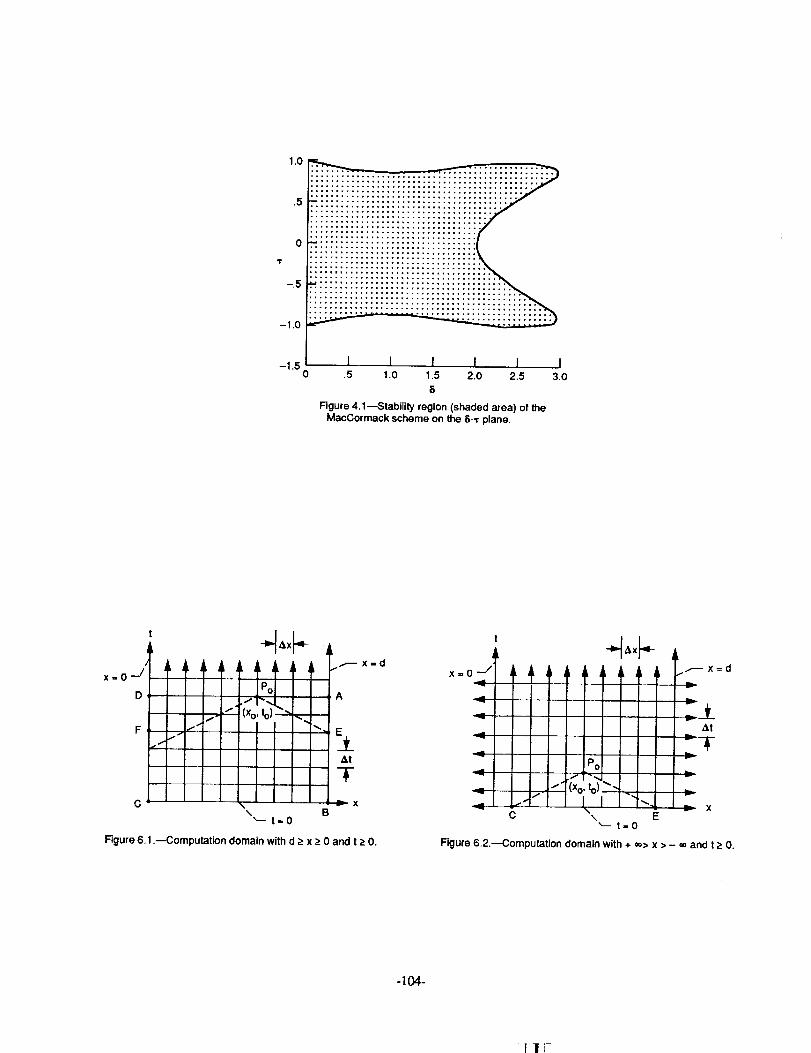
1.0
.5
0
'r
-,5
-1.0
-1.50
I I I I I.5 1.0 1.5 2.0 2.5
8
Figure 4.1_Stability region (shaded area) of theMacCormack scheme on the 8-_ plane.
I3,0
L
x=O --j
C
Po
t (Xo,to)"-..
\ B_-- t-O
L
., ,,--- x-dx=O --/
A
E._tAt
T =
Figure 6.1 .--Computation domain with d ;_x _ 0 and t > O.
!Po
! l"-,,,J ,,t- (Xo.to) .
___.-" I IC \
_x=d
' _ dLtv
v
v
E"-- t=O
Figure 6.2.-computation domain with + => x • - =oand t > O.
-]04-
111-

0
m
E
-1
-2
-3
-4
-5
[3
ii
iPTese_t atgorith, Tn.MctcCo'rTn.aclc sch, eTr_e
!L e ctpfrog/'DzLf ort-FrcLTzlc e t
I
0.00 0.05 O. 10 O. 15 0.20
Courant ntz_nSeT, "r
Figure 7.1--Accuracy of test problems in Set #1 (T - 30&t).
0.25
-105-

0
E
-1
-2
-3
-50.00
[11
llaH|idldggOB:aggBLH_LJ_
........................... o(iPO ....................................................................
.
:o
• iPTese_ct algoritlzm
[] iMctcCormaclc schemea iLeapfrogffDufort-Y.ankel
O.
I
0.05 O. 10 O. 15 0.20
Courant number, T
0.25
Rgure 7.2_ccuracy of bsst problems in Set #2 (T - 30At).
-106-
-_1[I-

i
E
-1
-2
-3
-4
-5
-6
iiiiii• iiiiiiiiiiiiii
i" :[3 MacCormaclc scheme:
[ iA Leapfrog/Dufort-Frc,,nkel
$oo
0.04 0.08
Couvant number, T
0.12
Figure 7.3--Accuracy of test problems In Set #3 (T - 60At).
'-107-

m
E
0
-1
-2
-3
-4
• : Present algorithm.[_i MacCormaclc scheme
a LeapfrogffDufort _Frankel
................... : ................... _ ................... _ ................... - ........... g.
: : : " •
: : : •
i E
g
......... -_ 0 I ............ , ................... , ...................
_eg• •
• •
so
|
-L .................. ; ................... : .................
|
0.0 0.2 0.4 0.6 0.8
Coura_t number, _-
Figure 7.4--Accuracy of test problems in Set #4 (T = 30ht).
1.0
-108-
Tli

E
0
-1
-2
-3
4
[]
• Present algorithm[] MacCormack scheme
a LeapfrogffDufort-_Frankel
0.0 0.2 0.4 0.6 0.8
Couvant number, "r
Figure 7.5--Accuracy of test problems In Set #5 (T = 2(1-b)/(3q3)).
1.0
-109-

0
-1
-2
[]
0.0 0.2 0,4 0.6 0.8 1.0
Courant number, T
Figure7.6--Accuracy of testproblemsin Set #6 (_ = 5(1-by(6_/3)).
-110-
1 II

-1
m
E
-z
-3
-4
-5
-6
®
]x
"" I................... , ................... r ..... 4_, ............ r ................... , ..................
! ix
d_
A
• !Present algorithwn@
• [] iMacCormack scheme
z_ iLeapfrog,f:Dufort-Frankel
i J
0.0 0.5 l.O 7.5 2.0 2.5
6
Figure 7.7--Accuracy of test problems in Set #7 (6 - 36&t).
-Ill-

10 z
101
................... , ................... . ................... o ................... . ................. .,_-
................... [ ................... . ................... , ................... , ..................
A
Z_
A:
Z_ •
...................i...............................i__# .......,.....!_........._.....
.................. ; .................. :_..,,,. :j,,__ _ _ : ,A
L_
A
0.0
I I
0.2 0.4 0.6 0.8
Cout'ant nU?T_6er, "r
Figure 7.8--Accuracy of test IXoblems tn Set #8 (_ - 30&t).
1.0
-112-
=1 1 ]

<N
\
\\
\
_-&x-_ \
\
,a _
"C3-_M' &t
t \\
t__xFigure 8.1 .--Boundary conservation element (&PQR).
t
X
Figure 8.2.--Hexagons as conservation elements.
_X
_gure 8.3.--Space-time E2 divided into conservation elements ofdifferent geometric shapes.
S Q
W U
Y
X
Figure 8.4.--Conservation element in space-time E3.
Imaginary axis
Real axis
Figure C.1 .--Geometric relations among the parameters r, _, pand _ defined by Eqs. (C.11) and (C.12).
-113-

Report Documentation PageSpace Admir_strst]on
1. Repeal No. I 2. Government Accession No.
INASA TM - 104495
4. Title and Subtitle
A New Numerical Framework for Solving Conservation Laws-TheMethod of Space-Time Conservation Element and Solution Element
7. Author(s)
Sin-Chung Chang and Wai-Ming To
9. Performing Organization Name and Address
National Aeronautics and Space AdministrationLewis Research Center
Cleveland, Ohio 44135-3191
12. Sponsoring Agency Name and Address
National Aeronautics and Space Administration
Washington, D.C, 20546- 0001
3. Recipient's Catalog No.
5. Report Date
August 1991
6. Performing Organizatio_ Code
8. Performing Organization Report No.
E- 6403
10. Work Unit No.
505- 62 - 52
11. Contract or Grant No.
13. Type of Report and Period Covered
Technical Memorandum
14. Sponsoring Agency Code
; 15. Supplementary Notes
Sin-Chung Chang, NASA Lewis Research Center; Wai-Ming To, Sverdrup Technolog3,, Inc., Lewis Research
Center Group, 2001 Aerospace Parkway, Brook Park, Ohio 44142. Responsible person, Sin-Chung Chang,(216) 433 - 5874.
16. Abstract
A new numerical framework for solving conservation laws is being developed. This new approach differs substantially
from the well established methods, i.e., finite difference, finite volume, finite element, and spectral methods, in bothconcept and methodology. It employs (1) a nontraditional formulation of the conservation laws in which space and timeare unified and treated on the same footing and (2) a nontraditional use of discrete variables such that numerical
marching can be carried out by using a set of relations that represents both local and global flux conservation. In this
paper, we also (1) explore the concept of a dynamic space-time mesh and the need for a unified treatment of physicalvariables and mesh parameters; (2) study the stability, dissipation and dispersion of the current scheme by using arigorous Fourier analysis; (3) develop a new error analysis technique that enables us to predict and interpret the numeri-
cal errors of the current and other classical schemes; (4) study the consistency and truncation error of the currentscheme; and (5) compare the errors of the numerical solutions generated by the current scheme and other classicalschemes.
17. Key Words (Suggested by Author(s))
Space-timeConservation element
Solution element
18. Distribution Statement
Unclassified - Unlimited
Subject Category 64
19. Secudty Classif. (of the report) 20. Secudty Classif. (of this page) 21. No. of pages
Unclassified Unclassified - 114-
NASAFORM1112(5OCT86 *Forsale by the NationalTechnical InformationService,Springfield,Virginia 22161
22. Price*
A04
1 1 I