norges teknisk-naturvitenskapeligeuniversitet

Conservation of phase space properties usingexponential integrators on the cubic Schrödinger

equationby

Håvard Berland, Alvaro L. Islas and Constance Schober

preprintnumerics no. 1/2006

norwegian university ofscience and technology

trondheim, norway

This report has URLhttp://www.math.ntnu.no/preprint/numerics/2006/N1-2006.pdf

Address: Department of Mathematical Sciences, Norwegian University of Science andTechnology, N-7491 Trondheim, Norway.

Conservation of phase space propertiesusing exponential integrators on the cubic

Schrödinger equation

Håvard Berland∗ Alvaro L. Islas† Constance M. Schober†

The cubic nonlinear Schrödinger (nls) equation with periodic boundary con-ditions is solvable using Inverse Spectral Theory. The “nonlinear” spectrum ofthe associated Lax pair reveals topological properties of the nls phase spacethat are difficult to assess by other means. In this paper we use the invarianceof the nonlinear spectrum to examine the long time behavior of exponentialand multisymplectic integrators as compared with the most commonly usedsplit step approach. The initial condition used is a perturbation of the unsta-ble plane wave solution, which is difficult to numerically resolve. Our findingsindicate that the exponential integrators from the viewpoint of efficiency andspeed have an edge over split step, while a lower order multisymplectic is notas accurate and too slow to compete.

1 Introduction

Exponential integrators have been popular in recent literature and they seem especiallyattractive in pde settings as a means of easily obtaining high order explicit schemes with-out step size restrictions for the time-integration. The notable property of exponentialintegrators is the use a splitting of the problem into a linear part, possibly rendering theproblem stiff, and a nonlinear part. The linear part is treated exactly, in an attempt toameliorate temporal step size restrictions imposed by possible stiffness inherent in the pdeproblem. However, experience with exponential integrators on long time scales for vari-ous pdes with a complicated phase space structure is not abundant. This paper examineswhether exponential integrators are a viable alternative for the time integration of pdes, bycomparing them with two other classes of time-integrators and by using the nls equationas a benchmark problem.

The nls equation is completely integrable with a rich phase space structure (i.e. stableas well as unstable solutions with homoclinic orbits). Typically the performance of anintegrator has been determined by examining the preservation of global invariants such asenergy and momentum. The nonlinear spectrum of the associated Lax pair of the pdeprovides a detailed description of the phase space and is invariant in time. Following [17],

∗Department of Mathematical Sciences, Norwegian University of Science and Technology, N-7491 Trond-heim, Norway, Havard.Berland@math.ntnu.no

†Department of Mathematics, University of Central Florida, Orlando, FL32816-1364, USA,aislas@mail.ucf.edu, cschober@mail.ucf.edu

1

we monitor the spectrum to assess how well the phase space is preserved by the variousintegrators. Section 2 outlines the necessary properties of the inverse spectral theory.

For Hamiltonian pdes possessing a multisymplectic structure (symplectic in both spaceand time), multisymplectic integrators preserve exactly a discrete version of the multisym-plectic structure [10]. For quadratic Hamiltonians, multisymplectic integrators preservethe local conservation laws exactly. Even though this is not the case for the nls equa-tion, multisymplectic integrators were shown to provide improved resolution of the localconservation laws and dynamical invariants [16, 17]. Compared to classical integrators(Runge–Kutta), multisymplectic integrators exhibited less drift in the conservation lawsover long time periods [17]. We include an implicit second order multisymplectic integratorfor comparison with the exponential integrators and it is found to be the most computa-tionally demanding integrator among those tested. Whether improved preservation of thestructural and geometric properties of the pde by multisymplectic integrators justifies theiradditional computational cost remains an open question.

Section 3 gives the necessary details of the spectral space discretization, which will beequivalent for all schemes included in this study. In Section 3.2 exponential integratorsare presented in a format including the majority of known exponential integrators, andspecifications of the exponential integrators used are given in coefficient function tableaus.We restrict our attention to explicit exponential integrators to facilitate speed and ease ofimplementation, and test the two integrators cfree4 and lawson4. The implementationhas used the matlab package described in [7] directly. A fourth order split step schemeobtained by Yoshida’s technique is included for comparison, as it is, in many ways, relatedto exponential integrators and it is also used fairly extensively in the physics community.We only included a multisymplectic integrator of order two as, even at this order, it turnedout to be computationally more intensive than the other integrators. Our final criteria forcomparing integrators is based on accuracy obtained for fixed cpu time, and thus it makessense to compare integrators with differing asymptotic order.

The numerical results are given in Section 4 where we examine how well the most criticalfeatures of the nonlinear spectrum are preserved. Knowledge of the properties of thenonlinear spectrum makes it possible to give simple criteria for determining whether anumerical result is acceptable or not. We present results in table form and conclude thatamong our integrators, cfree4 seems to be the most reliable and cpu effective choice forour problem.

The nonlinear Schrödinger equation

The periodic focusing nonlinear Schrödinger (nls) equation

ut = iuxx + i2|u|2u, (1)

u(x+D, t) = u(x, t), is an infinite dimensional integrable Hamiltonian system with Hamil-tonian

H(u, u∗) =∫ D

0

(|ux|2 − |u|4

)dx. (2)

The (complex) solution u(x, t) represents the slow space-time evolution of the envelope ofa carrier signal, and has important applications in nonlinear optics, deep water waves andalso plasma physics. The wave equation (1) bears its name because it corresponds to thequantum Schrödinger equation with 2|u|2 as the potential.

An important physical prediction of the NLS equation is the Benjamin–Feir or modula-tional instability for periodic boundary conditions [4]. An example of this is provided by

2

the plane wave solution,u(x, t) = ae2i|a|2t. (3)

which has M linearly unstable modes with growth rates σ2n = µ2

n(µ2n − 4a2), µn = 2πn/D,

provided0 < (πn/D)2 < |a|2 (4)

is satisfied (the number M of unstable modes is the largest integer satisfying 0 < M <|a|D/π). That is, the plane wave is unstable with respect to long wavelength perturbations.

In the numerical experiments we consider multi-phase solutions whose initial data isobtained by perturbing the plane wave solution,

u(x, 0) = a(1 + ε eiψ cos(µnx)

), (5)

where a = 12 , µn = 2πn

D and D = 4√

2π is the length of the spatial domain. Typically, thestrength of the perturbation ε is chosen to be 0.1, ψ = 0 and n = 1. For the given spatiallength D, the plane wave has two unstable modes, thereby the initial condition is coinedthe two-mode case. Increasing the spatial period results in more unstable modes, makingthe problem numerically harder.

2 The inverse spectral method

In [28], the nls equation (1) was shown by Zakharov and Shabat to be completely integrable(with infinite sequences of commuting flows and common conservation laws) and solvableby inverse scattering theory for rapidly decreasing initial data on the infinite line. Specialsolutions such as solitons, which are localized wave packets (envelope solutions for thenls equation) that survive collisions with one another, were proven to exist in this case.More generally, inverse spectral theory provides a method, the analog of the whole-lineinverse scattering theory, for solving the nls equation on periodic domains. Its, Kricheverand Kotlarov used inverse spectral theory and methods of algebraic geometry to obtainN -phase solutions of the periodic nls equation, expressible in terms of Riemann thetafunctions [18, 20, 3].

2.1 Lax pair and characterization of the spectrum

The inverse scattering and spectral methods may be viewed as a generalization of Fouriermethods for solving linear pdes. Briefly, the complete integrability of the nls equation isestablished by using the associated Lax pair of linear operators defined by [28]:

L(x)φ = 0 and L(t)φ = 0, (6)

where

L(x) =(

ddx + iλ −uu∗ d

dx − iλ

)and L(t) =

(ddt + i[2λ2 − |u|2] −2λu− iux

2λu∗ − iu∗xddt − i[2λ2 − |u|2]

)(7)

The coefficients u(x, t) are periodic in x, u(x+D, t) = u(x, t), λ is the spectral parameter,and φ is the eigenfunction. The nls equation arises as the solvability or compatibility con-dition for these operators, i.e., φxt = φtx if and only if u(x, t) satisfies the nls equation (1).

The first step in solving the nls equation is to calculate the direct spectral transform ofthe initial data, i.e. to determine the spectrum of L(x), which is analogous to calculatingthe Fourier coefficients in Fourier theory. Next, time evolution is performed on the “spectral

3

data” using L(t). Finally the inverse spectral transform is calculated in order to recoverthe waveform at a later time.

The direct spectral transform and its inverse provide a one-to-one correspondence be-tween solutions of the nls equation and the spectral data. The spectral data consists oftwo types of spectrum of L(x); the periodic eigenvalues λj and the Dirichlet eigenvalues µj(to be defined below). The direct spectral transform consists of computing (λj , µj) fromu(x, t). A fundamental property is that the periodic eigenvalues λj are invariants of thenls flow whereas the Dirichlet spectrum flows in both x and t. The time dependence ofµj(x, t) is generated by L(t) and is equivalent to the dynamics of the nls flow since L(x)

and L(t) are compatible. The inversion formula for N -phase solutions of the nls is givenby the trace formula [18]:

iuxu

=2N∑j=1

λj − 2N−1∑j=1

µj .

For periodic potentials the spectrum is obtained using Floquet theory. This spectral anal-ysis is similar to that of the time-independent Hill’s operator, with the main differencethat L(x) is not self-adjoint. The spectrum of u,

σ(u) =λ ∈ C | L(x)φ = 0, |φ| bounded ∀x

, (8)

can be expressed in terms of the transfer matrix M(x + D;u, λ) across a period, whereM(x;u, λ) is a fundamental solution matrix of the Lax pair (7). Introducing the Floquetdiscriminant ∆(u, λ) = Trace [M(x+ L;u, λ)], one obtains

σ(u) = λ ∈ C | ∆(u, λ) ∈ R, −2 ≤ ∆(u, λ) ≤ 2 . (9)

The distinguished points of the periodic/antiperiodic spectrum are where ∆(u, λj) = ±2,and are categorized as

(a) Simple points λsj | d∆dλ 6= 0,

(b) Double points λdj | d∆dλ = 0, d2∆

dλ2 6= 0.

The Floquet discriminant functional ∆(u, λ) is invariant under the nls flow and encodesthe infinite family of constants of motion of the nls (parametrized by the λj ’s). While theλj ’s are equivalent to a set of invariant action variables, the µj ’s (which are the zeros ofthe M12 entry of the transfer matrix and are not invariant) provide the conjugate anglevariables.

The Floquet spectrum (9) of a generic nls potential consists of the entire real axisplus additional curves (called bands) of continuous spectrum in the complex plane whichterminate at the simple points λsj . N -phase solutions are those with a finite number ofbands of continuous spectrum. Double points can be thought of as the coalescence of twosimple points and their location is particularly significant. The order and location of theλj completely determine the spatial structure and nonlinear mode content of nls solutionsas well as the dynamical stability as follows [12, 13]:

(a) Simple points correspond to stable active degrees of freedom.

(b) Double points label all additional potentially active degrees of freedom.

Real double points correspond to stable inactive (zero amplitude) modes. Complex doublepoints correspond to the unstable active modes and parametrize the associated homoclinicorbits.

4

The N -phase quasiperiodic solutions of the nls equation have the form [3, 18, 20],

u(x, t) = u0ei(k0x−ω0t) Θ(W−|τ)Θ(W+|τ)

, (10)

where Θ is the Riemann theta function, W± = (W±1 , . . . ,W

±N ), and the phases evolve

according to W±j = (κjx + Ωjt + θ±j ). The external phase as well as the wavenumbers

κj and frequencies Ωj are expressible in terms of algebraic-geometric data including thebranch points of the associated Riemann surface (namely, the simple points λsj of theFloquet spectrum). The entire x and t dependence of an N -phase solution is capturedby odes for the µj ’s. Essentially these odes linearize via the classical Abel–Jacobi mapassociated with the Riemann surface. The phases W±

j in the action-angle description ofthese solutions are the images of µj(x, t) under the Abel–Jacobi map.

In terms of the nls phase space, the values of the actions λj fix a particular level set.The level set defined by u is then given by, Mu ≡ v |∆(v, λ) = ∆(u, λ), λ ∈ C. Typically,Mu is an infinite dimensional stable torus. However, the nls phase space also containsdegenerate tori which may be unstable. If a torus is unstable, its invariant level set consistsof the torus and an orbit homoclinic to the torus. These invariant level sets, consistingof an unstable component, are represented, in general, by complex double points in thespectrum [13].

In our experiments we implement the first step of the inverse spectral method and appealto the invariance of the λj ’s to evaluate the ability of the various numerical schemes topreserve the nls phase space structure. The nonlinear spectrum for the Lax pair (7) iscomputed numerically using Fortran software at each timevalue of the solution. In ourcase, only the λj ’s where ∆ = ±2 are necessary. The discriminant function ∆ is obtainedby a direct nonlinear spectral transform, solving the overdetermined system of odes (inthe variable x) given by the Lax pair for the given numerical solution u(x, t). The zerosof ∆ = ±2 are then obtained with a root solver using Muller’s method as in [21]. Thespectrum itself is calculated with an accuracy of O(10−8) which is sufficient for our results.

2.2 Perturbation of the plane wave

The simplest example of an N -phase solution of the nls equation is the plane wave solu-tion (3). In this case, the Floquet discriminant is given by ∆(a, λ) = 2 cos(

√a2 + λ2D)

and thus the spectrum consists of the entire real axis and the band [−ia, ia]. At ±ia thereis a pair of simple periodic/antiperiodic eigenvalues and there is an infinite sequence ofdouble points,

λ2j = (jπ/D)2 − a2 (11)

for j ∈ Z, of which 2baD/πc = 2M are pure imaginary double points and the remainingare real. The condition for a complex double point is exactly the condition for a mode tobe linearly unstable (compare with (4)). However, in contrast to inverse spectral theory,linear analysis does not provide any answers to what happens to the solution on a longtime-scale.

When a = 0.5 and D = 4√

2π in (3), M = 2 and λ1 and λ2 are complex double points(since the spectrum is symmetric with respect to the real axis we restrict our considerationto Imλ ≥ 0). It is difficult in advance to predict the time of failure using only physical dataor a few global constants. For the family of initial data (5), as the energy levels are variedslightly there are alternating windows of stable and unstable tori. As a consequence, wehave found that the λj ’s, which determine the geometry of the level sets, are the significantquantities to preserve [17].

5

Im

Re

Band of real ∆(λ)Double point

λd

2

λd

1

ia

(a) Plane wave, unperturbed.

λ−

2

Im

Re

∆(λ) = 2

Band of real ∆(λ)

Gap G1, size ε

Gap G2, size ε2

∆(λ) = −2λ

+

1

λ−

1

λ+

2

(b) Perturbed, two-mode solution.

Figure 1: The spectrum (9) for (a) the plane wave (3) and (b) the perturbed plane wavedata (5). The perturbation of strength ε opens up the two double points of the plane wavespectrum (a) and yields the perturbed spectrum (b) with two gaps corresponding to twosemi-stable modes in the solution (see Figure 2). Real double points are not shown.

Assuming u = u(0) + εu(1) + · · · , λ = λ(0) + ελ(1) + · · · , and φ = φ(0) + εφ(1) + · · · , thespectrum of initial data (5) can be calculated via perturbation analysis. Substituting theseexpansions into (7), the λ(0)

j are given by (11) and the corrections at O(ε) are [2]

(λ

(1)j

)2=

a2

16λ2j

(e−iφ − 1

a2 (jπ/D + λj)2 eiφ

)·(e−iφ − 1

a2 (−jπ/D + λj)2 eiφ

)j = n

0 j 6= n

(12)

At O(ε) there is a correction only to the double point λ(0)j , (j = n), which resonates with

the perturbation. The other double points do not experience an O(ε) correction.The behavior of the correction λ(1)

j , (j = n), depends on whether the double point λ(0)j

is real or imaginary:

(λ

(1)j

)2=

− a2

4λ2jsin(φ+ θ) sin(φ− θ) for λj imaginary

− a2

8λ2j

[cos 2φ+ 1− 2(jπ/D)2/a2

]for λj real

where tan θ = Im(λj)D/(jπ). Since initial data (5) is for a solution even in x, the spectrumhas an additional symmetry with respect to the imaginary axis. This is reflected in thecorrection λ(1)

j which, for imaginary double points, is either real, zero or pure imaginary [2]depending on the choice of ψ in the perturbed potential, i.e. imaginary double pointscan split into either crosses or gaps in the spectrum. This is a realization of the saddlestructure of the real part ∆(u, λj) when λj is imaginary. More generally, if the potentialis noneven in x, the correction λ(1)

j is fully complex and the double point can split in anydirection, yielding an asymmetric version of a gap state.

For real double points, the correction λ(1)j can only be imaginary. Gaps cannot appear

on the real axis in the spectrum of L(x). Hence the situation with real double points isvery different from that of imaginary double points. Splitting of real double points onlyintroduces additional degrees of freedom into the spatial structure but does not introducean instability as homoclinic manifolds are not associated with them. At the next orderonly the double points λj , (j = 2n), experience an O(ε2)-splitting. A full determination ofthe splitting at higher order is given in [2] and in the non-even case in [1].

6

PSfrag replacements

x

time

|u(x

,t)

|2

-8-6-4-202468

-50

5

02040

010

2030

40

0.51

1.52 0.5

11.5

2

Figure 2: The surface |u(x, t)|2 of the nonlinear Schrödinger equation with initial condi-tion (5). The center mode around x = 0 corresponds to gap G1 in Figure 1b, and thesecond mode appearing around x = ±3 in the |u(x, t)|2-plot corresponds to gap G2 inFigure 1b.

The Floquet spectrum for initial data (5), with ψ = 0 and n = 1 is shown in Figure 1b.The corrections to λ1 and λ2, as determined by (12), are pure imaginary and gaps G1 andG2 open in the spectrum with sizes of order ε and ε2, respectively [2]. The double pointλj splits into λ±j and the gap Gj = λ+

j −λ−j . The first gap corresponds to the center mode

in Figure 2 and from λ±1 the spatial and temporal frequencies of the mode are determined.Similarly λ±2 (corresponding to the smaller gap of size ε2) determine the wave number andfrequency of the second mode which appears symmetrically on both sides. If the ratio ofthe two temporal frequencies is a rational number, the initial condition will recur in finitetime.

3 Numerical integrators

3.1 Space discretization

The instability of the nls equation which we are examining occurs only for periodic bound-ary condition, thus it is reasonable to restrict our attention to spectral spatial discretiza-tions making use of the fast Fourier transform. The spatial resolution is equivalent for allof the schemes considered, so the differences in performance are attributable to the timeintegrators.

Let

u(k, t) = F(u(x, t)) =1D

∫ D/2

−D/2u(x, t)e−νkx dx

with k ∈ Z and νk = 2πiD k be the Fourier transform of u(x, t). The inverse Fourier transform

is

u(x, t) = F−1(u(k, t)) =∞∑

k=−∞u(k, t)eνkx.

In Fourier space, equation (1) then takes the form of an infinite system of first order ODEs

ut(k, t) = iν2k u(k, t) + 2i

∣∣F−1(u(k, t))∣∣2 u(k, t) k ∈ Z, t ≥ 0

u(k, 0) = F(u(x, 0)). (13)

The spatial discretization now consists of truncating (13) to NF/2 ≤ k ≤ NF/2 − 1, andthe resulting system of dimension NF is then solved by the integrators mentioned below.

7

3.2 Exponential integrators

Exponential integrators are a class of integrators that emerged from an improved abilityin numerical software to compute the matrix exponential in a reasonable amount of time.Recent developments [5, 11, 15, 22] have yielded an abundance of possibilities with regardsto choice of scheme (see for instance [7] and the accompanying source code for a listing).In this study we examine the performance of the class of exponential integrators; thus, theparticular choice of exponential integrator is of less importance. After numerous initialnumerical tests, we have chosen cfree4 as “the” exponential integrator in this report. Itgives the best overall performance for our problem as measured by the global error andthe preservation of invariants over long integration intervals.

An s-stage explicit exponential integrator of Runge–Kutta type for the system of ordi-nary differential equations

y(t) = Ly(t) +N(y, t), y(0) = y0 ∈ Rn (14)

where L is linear and N(y, t) is a (possibly) nonlinear function, is the procedure

Yi =s∑j=1

aij(hL)hN(Yj , t0 + cjh) + exp(cihL)y0 (15a)

y1 =s∑i=1

bi(hL)hN(Yi, t0 + cih) + exp(hL)y0 (15b)

in which Yi, i = 1, . . . , s, are internal stages and y1 is the final approximation of y(t1) =y(t0+h). This format extends the format for Runge–Kutta schemes in that the coefficientsaij and bi are now analytic functions in the matrix L.

In short, the main properties of an exponential integrator are (i) when the linear part Lis zero, we recover the underlying Runge–Kutta-scheme, and (ii) when N ≡ 0, exponentialintegrators compute the exact solution. The coefficient functions aij(z) and bi(z) (z = hL)are usually listed in a tableau similar to the Butcher tableau for Runge–Kutta schemes.For cfree4, the functions are

0 112

12ϕ1,2 ez/2

12

12ϕ1,2 ez/2

1 12ϕ1,2(ez/2 − 1) ϕ1,2 ez

12ϕ1 − 1

3ϕ1,213ϕ1

13ϕ1 −1

6ϕ1 + 13ϕ1,2 ez

(16)

where

ϕ`(z) =1

(`− 1)!

∫ 1

0e(1−θ)zθ`−1 dθ, ` = 1, 2, . . . (17)

andϕi,j = ϕi(cjz), i = 1, . . . and j = 1, . . . , s. (18)

For ` = 1, 2, 3 (and for z 6= 0) the functions are

ϕ1(z) =ez − 1z

, ϕ2(z) =ez − z − 1

z2, and ϕ3(z) =

ez − z2/2− z − 1z3

.

There is a singularity at z = 0 that could potentially lead to cancellation errors for smalltime steps. In order to avoid this in our experiments, these so called ϕ functions are

8

evaluated by scaling the argument z, using a Padé approximant of ϕ`, and squaring theresult. Details for this are presented in [7] and further analyzed in [8, 19].

Stiff order analysis of exponential integrators was introduced as an analytical tool in [15]which addresses the convergence of exponential integrators for semi-linear parabolic partialdifferential equations. To obtain order p convergence in that case, independently of spatialresolution, stiff order p for the exponential integrator is required. Stiff order conditionsrepresent an additional set of order conditions, including the classical order conditions asa special case. The cfree4 scheme is only of stiff order 2, but still outperformed the otherschemes in the initial study, including expensive schemes with high stiff order, though onlymarginally in some cases.

The report [6] is a study of two fourth order exponential integrators on the nonlinearSchrödinger equation, one Lawson integrator with stiff order 1, and etd4rk from [11] withstiff order 2. Some effects (exhibited through order reduction) were attributable to low stifforder of the Lawson integrators, possibly also connected to preservation of fixed points, acondition equivalent to stiff order 2. Given sufficient spatial smoothness of the nonlinearfunction, and sufficient smoothness of the initial condition, high stiff order seemed lessimportant. Also in [6], connections between the Lawson type and split step integrators areindicated, and it is in this respect that the we include the Lawson integrator of order 4but stiff order 1, lawson4, with tableau

0 112

12ez/2 ez/2

12

12 ez/2

1 ez/2 ez16ez 1

3ez/2 13ez/2 1

6 ez

. (19)

Both cfree4 and lawson4 reduce to the same classical fourth order Runge–Kuttascheme when the linear part is zero.

In the spectral space discretization, the matrix L in (14) for (13) becomes diagonal withelements

Lkk = iν2k = −ik2/8, k = −NF/2, . . . , NF/2− 1. (20)

The nonlinear function N in (14) becomes

N(u(k, t), t) = 2i∣∣F−1(u(k, t))

∣∣2 u(k, t). (21)

Our implementation uses fixed step sizes for all schemes, and as the linear part is time-independent, the functions eciz and ϕi,j are computed only at time zero of the integrationand cached for the subsequent integration steps. Thus, the cost of evaluating the expo-nential and the ϕ functions are amortized over long integration intervals.

3.3 Second order multisymplectic spectral

The multisymplectic formulation for the nonlinear Schrödinger equation was introducedin [10], as an integrator being symplectic in both time and space. Multisymplectic integra-tors preserve exactly a discrete version of multisymplecticity. If the Hamiltonian functionS(z) is space and time independent, the pde will possess local energy and momentumconservation laws. In addition, if S(z) is quadratic in z, a multisymplectic integrator willpreserve exactly these local conservation laws and, in the periodic case, the associatedglobal conservation laws.

9

Although the Hamiltonian for the nls equation is space and time independent, it is notquadratic and thus only multisymplecticity is exactly conserved in this case. Nevertheless,multisymplectic integrators have been reported to preserve the conservation laws betterthan classical Runge–Kutta schemes [17].

We will first show the multisymplectic formulation for a finite difference discretizationof a pde, then we see how it simplifies when using a spectral discretization in space.

Equation (1) can be written in multisymplectic form by letting u = p+iq and augmentingthe phase space with the variables v = px and w = qx. The system obtained is

qt − vx = 2(p2 + q2)p

−pt − wx = 2(p2 + q2)qpx = v

qx = w

(22)

A Hamiltonian pde is defined as multisymplectic if it can be written in the form

Mzt +Kzx = ∇zS(z)

where M and K are skew-symmetric matrices, and S is a smooth function of the statevariable z. Formulation (22) of the nonlinear Schrödinger equation is multisymplecticprovided

z =

pqvw

, M =

0 1 0 0−1 0 0 00 0 0 00 0 0 0

, K =

0 0 −1 00 0 0 −11 0 0 00 1 0 0

,

and S(z) = 12

((p2 + q2)2 + v2 + w2

).

The multisymplectic conservation law is

ωt + κx = 0 (23)

where ω and κ are alternating forms

ω(U, V ) = 〈MU,V 〉 = V TMU and κ(U, V ) = 〈KU, V 〉 = V TKU (24)

for two solutions, U and V , of the variational equation associated to the pde (22) [10]. Anintegrator of the system (22) is multisymplectic if and only if a discretized version of (23)is preserved exactly.

The centered cell discretization [10] is a centered difference approximation in space to(22), and implicit midpoint in space, which can be proven to be a multisymplectic scheme.However, in our periodic case, the finite difference discretization in space is inferior to aspectral space discretization, and thus, it has not been included in the numerical tests inthis report.

Instead, the centered cell discretization is modified to use a spectral discretization inspace. Approximation of space differentiation can be seen as multiplication by the spectraldifferentiation matrix D [14],

dudx

≈ Duk, uk ≈ u(xk), D =

(−1)j−k πD cot π

D (xj − xk) if j 6= k

0 if j = k(25)

Replacing all space derivatives in (22) with spectral differentiation using D, and modifyingthe multisymplectic conservation law (23) accordingly, in [17] the authors prove that thistogether with implicit midpoint in time yields a multisymplectic scheme for the nonlinearSchrödinger equation. We denote this scheme msspectral2. The implicit equation ateach time step is solved numerically using a simplified Newton iteration.

10

3.4 Fourth order split step scheme

Split step schemes have been used for a long time for integrating the nonlinear Schrödingerequation in physical applications. In our context, [25] is an early reference to the typeof scheme. Taha and Ablowitz [24] give an extensive survey of the prime integrators forthe numerical solution of the nonlinear Schrödinger equation, and conclude that Tappert’ssplit step Fourier scheme [25] is in most cases superior to the other schemes considered.The paper [26] investigates numerical aspects of the basic first order split step Fouriermethod using linearization techniques.

For the split step Fourier method to be comparable to the fourth order exponentialintegrators used, we first construct a second order scheme by using a Strang splittingtechnique [23] and the same splitting as for exponential integrators. Let Φh

RK4C(y(t0)) bethe approximation to y(t0 + h) produced by Kutta’s classical fourth order scheme for theproblem y(t) = N(y, t). Then a Strang splitting scheme for (14) is

ΦhSS2(y0) = Φh/2

RK4C exp(hL) Φh/2RK4C(y0) (26)

with L and N given by (20) and (21). Then we use Yoshida’s formula

ΦSS4(y0) = Φc1hSS2 Φc0h

SS2 Φc1hSS2(y0) (27)

to construct a fourth order split step scheme from the second order Strang scheme, wherec0 = −21/3

2−21/3 and c1 = 12−21/3 [27]. Scheme (27) will be denoted splitstep4 in the remainder

of this paper.splitstep4 is picked as a representative and well-studied scheme within the class of

split step schemes for the nonlinear Schrödinger equation. However, recently symplecticpartitioned Runge–Kutta schemes have been constructed for the nonlinear Schrödingerequation which maybe could outperform the splitstep4 scheme used here, as reportedin [9]. In further studies, these new split step schemes should also be compared to expo-nential integrators.

4 Numerical results

The nls (1) equation with a perturbed plane wave solution as the initial condition (5) hasbeen integrated with various choices of the spatial discretization parameter NF and thetemporal step size h. Our aim is to determine the time length for which the numericalsolution is valid, where the validity is determined by how well the nonlinear spectrum ispreserved, and thereby judge the chosen integrators. Table 1 indicates the length of timefor which the numerical solution was accepted according to criteria based entirely on thenonlinear spectrum and constitutes the main result from this work.

4.1 Preservation of nonlinear spectrum

The spectrum of the nls equation is invariant in time, but the truncation errors incurredby the numerical schemes result in numerical solutions that can be viewed as the exactsolutions of corresponding perturbed equations, for which the spectra evolve in time. Thus,the positions of the single/double points and the bands of real discriminant ∆(u, λ), com-puted by software briefly described in Section 2.1, will in general vary in time. It has beencustomary in similar studies to monitor conservation of momentum, energy and norm.These three quantities are expressible in terms of the nonlinear spectrum, but alone fail todescribe all the properties of the spectrum.

11

h = 10−1 h = 10−2 h = 10−3 h = 10−4

cfree4 6.9 (1) 6.9 (1) 6.9 (1) 6.9 (1)

lawson4 6.9 (1) 6.9 (1) 6.9 (1) 6.9 (1)

splitstep4 6.7 (1,2) 6.9 (1) 6.9 (1) 6.9 (1)

msspectral2 26.2 (1) 6.9 (1) 6.9 (1) 6.9 (1)

(a) NF = 64

h = 10−1 h = 10−2 h = 10−3 h = 10−4

cfree4 90.1 (1) 157.9 (1) 157.9 (1) 157.9 (1)

lawson4 6.8 (2) 157.9 (1) 157.9 (1) 157.9 (1)

splitstep4 7 (1,2) 2049 (r) 157.9 (1) 157.9 (1)

msspectral2 5.9 (2) 207.8 (1) 158 (1) 157.9 (1)

(b) NF = 128

h = 10−1 h = 10−2 h = 10−3 h = 10−4

cfree4 90.3 (1) 3165 (r) > 10000 > 10000lawson4 6.7 (2) 1891 (r) > 10000 > 10000splitstep4 7.1 (1,2) 2400 (r) > 10000 > 10000msspectral2 5.9 (2) 207.6 (2) 1426 (r) > 500

(c) NF = 256

h = 10−1 h = 10−2 h = 10−3 h = 10−4

cfree4 90.3 (1) 3166 (r) > 10000 > 10000lawson4 6.7 (2) 1993 (r) > 10000 > 10000splitstep4 7.1 (1,2) 907.4 (r) 1479 (r) > 10000msspectral2 5.9 (2) 109.8 (2) 1426 (r) n/a

(d) NF = 512

Table 1: Time until numerical solution fails. Symbols next to numbers denote reason forfailure.

The initial condition is a perturbation of an unstable state, and the numerical challengeis to balance near the border of this instability. We allow for discrepancies that are smallenough not to excite any of the unstable modes, or said differently, we avoid topologicalchanges to the spectral configuration.

If the gap size becomes zero (gap closure) we obtain a degenerate double point, as inthe plane wave solution ε = 0, Figure 1a, and the solution may then undergo a homocliniccrossing, entering a completely different state. A typical scenario after a gap closure is thateigenvalues at the end of the bands λ±j obtain a nonzero real part and the mode enters a“cross” state. This corresponds to the solution having different spatial structure. Spatialsymmetry is also typically lost as the modes may start to drift spatially. As symmetry isnot enforced in the numerical solutions, accumulation of non-symmetric round-off errorsmay eventually ruin the numerical solution. In the non-symmetric (non-even) case, it isseen in [1] that the real part of the eigenvalues may grow without being initiated by ahomoclinic crossing. The gap sizes and the magnitude of the real part of the single pointshave therefore been used as the main indicators of the validity of the numerical solution.

The numerical solution at time T is accepted given that the topological properties of thespectrum have remained unchanged for 0 ≤ t ≤ T . Let

Gj(t) = λ+j (t)− λ−j (t), j = 1, 2, (28)

12

denote the gap (complex valued) Gj at time t with reference to Figure 1a.We monitor the deviations in the spectrum λ±j , examining the real and imaginary com-

ponents independently. The precise requirements used are

1100

|ImGj(0)| < |ImGj(t)| < 100|ImGj(0)| for j = 1, 2,

|ReGj(0)| < 5 · 10−5.(29)

The smallest t for which one of these requirements are not met in a given scenario isprinted in Table 1. The specific numbers 100 and 5 · 10−5 have been chosen to reveal thesignificant differences between the integrators in preserving the vital features of the phasespace structure, that is, allowing everything but topological changes in the spectrum. Thenumbers must also be comparable to the eigenvalue accuracy of the spectrum computation,which in our case has been O(10−8). Also note that |ImGj(t)| never reached its upperlimit before the solution was invalidated by the other requirements in our experiments.

Based on the numerical solutions and the accompanying spectra produced, we find thatthe nonlinear spectrum evolves in four different ways.

(1) Gap 1 closes (|ImG1| ≈ 0). Subsequently, |ReG1| is nonzero. The numerical solutionis said to “cross” a homoclinic orbit and enter a different state, often with the centermode spatially shifted half the domain length. This is exemplified in Figure 3.

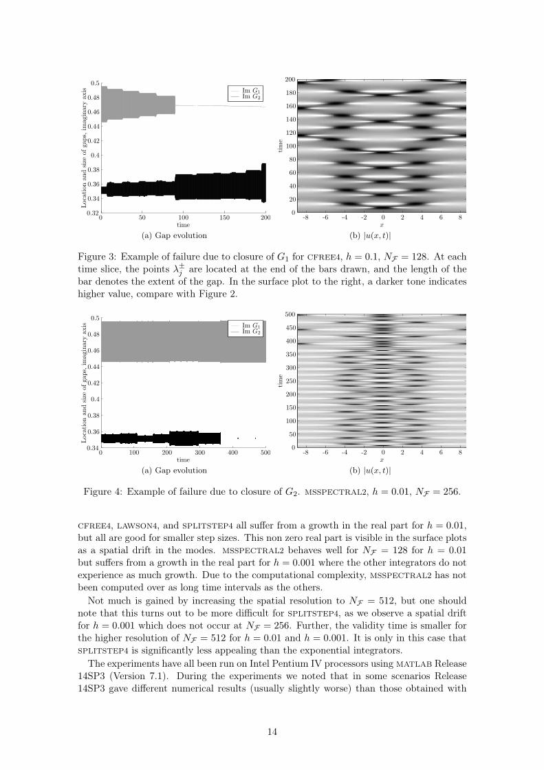
(2) Gap 2 closes (|ImG2| ≈ 0). Subsequently, |ReG2| is nonzero. Gap 2 corresponds tothe antiperiodic mode appearing on both sides of the center mode, and also experi-ences spatial shift during gap closure and homoclinic crossing. This is exemplified inFigure 4.

(1,2) Both gaps close. This is similar to the two cases above, but here both gaps closeduring the time span defined by one peak of a mode. In the scenarios included here,this has been the onset of computational chaos in the numerical solution. This isexemplified in Figure 5.

(r) |ReG2| becomes nonzero, without any gap closures. This only happens on long timescales, and is due to accumulation of non-symmetric round-off errors. The sign of λ+

2

and λ−2 is always different, and the sign of λ+2 determines the direction (right or left)

the corresponding mode will travel in phase space. The real extent determine thespeed of spatial drift. In some of the cases, this case is followed by |ReG1| becomingnon-zero as well. This is exemplified in Figure 6.

It is evident from the data in Table 1 that sufficient spatial resolution is a first prerequisitefor a valid long-time computation. Using only NF = 64, G1 closes during the first peakof the center mode for all integrators independent of temporal step size h, except formsspectral2, which fails at the second center mode peak.

Increasing spatial accuracy to NF = 128 one can integrate for a longer period of time,but still, for most configurations G1 closes early. Of special interest is the exceptional resultof splitstep4 for h = 10−2, where gap closures are avoided but the accumulation of non-symmetric round-off error eventually grows large enough to destroy the solution. However,finer experiments indicated that there is a small window for h in which better spectrumpreservation is achieved for this integrator. In general, for NF = 128 and h ≤ 0.01, thereare no significant differences in the performance of the various schemes.

At NF = 256 the spatial resolution is sufficient to reveal differences in the time-integration. If h ≤ 0.001, all of the schemes are able to integrate for as long as we tested.

13

PSfrag replacements

Loca

tion

and

size

ofgaps,

imagin

ary

axis

time

Im G2

Im G1

0 50 100 150 2000.32

0.34

0.36

0.38

0.4

0.42

0.44

0.46

0.48

0.5

(a) Gap evolution

PSfrag replacements

x

tim

e

-8 -6 -4 -2 0 2 4 6 80

20

40

60

80

100

120

140

160

180

200

(b) |u(x, t)|

Figure 3: Example of failure due to closure of G1 for cfree4, h = 0.1, NF = 128. At eachtime slice, the points λ±j are located at the end of the bars drawn, and the length of thebar denotes the extent of the gap. In the surface plot to the right, a darker tone indicateshigher value, compare with Figure 2.

PSfrag replacements

Loca

tion

and

size

ofgaps,

imagin

ary

axis

time

Im G2

Im G1

0 100 200 300 400 5000.34

0.36

0.38

0.4

0.42

0.44

0.46

0.48

0.5

(a) Gap evolution

PSfrag replacements

x

tim

e

-8 -6 -4 -2 0 2 4 6 80

50

100

150

200

250

300

350

400

450

500

(b) |u(x, t)|

Figure 4: Example of failure due to closure of G2. msspectral2, h = 0.01, NF = 256.

cfree4, lawson4, and splitstep4 all suffer from a growth in the real part for h = 0.01,but all are good for smaller step sizes. This non zero real part is visible in the surface plotsas a spatial drift in the modes. msspectral2 behaves well for NF = 128 for h = 0.01but suffers from a growth in the real part for h = 0.001 where the other integrators do notexperience as much growth. Due to the computational complexity, msspectral2 has notbeen computed over as long time intervals as the others.

Not much is gained by increasing the spatial resolution to NF = 512, but one shouldnote that this turns out to be more difficult for splitstep4, as we observe a spatial driftfor h = 0.001 which does not occur at NF = 256. Further, the validity time is smaller forthe higher resolution of NF = 512 for h = 0.01 and h = 0.001. It is only in this case thatsplitstep4 is significantly less appealing than the exponential integrators.

The experiments have all been run on Intel Pentium IV processors using matlab Release14SP3 (Version 7.1). During the experiments we noted that in some scenarios Release14SP3 gave different numerical results (usually slightly worse) than those obtained with

14

PSfrag replacements

Loca

tion

and

size

ofgaps,

imagin

ary

axis

time

Im G2

Im G1

0 10 20 30 40 50 600

0.1

0.2

0.3

0.4

0.5

0.6

0.7

(a) Imaginary part of gap sizes as a function of time

PSfrag replacements

x

tim

e

-8 -6 -4 -2 0 2 4 6 80

10

20

30

40

50

60

(b) |u(x, t)|

Figure 5: Example of failure due to closure ofG1 andG2. splitstep4, h = 0.01, NF = 256.Development of computational chaos as observed here is typical for splitstep4.

PSfrag replacements

Rea

lpart

ofgapsi

zes

time

|Re G2||Re G1|

0 1000 2000 3000 4000 500010−10

10−9

10−8

10−7

10−6

10−5

10−4

10−3

(a) Real part of gap sizes as a function of time

PSfrag replacements

x

tim

e

-8 -6 -4 -2 0 2 4 6 80

500

1000

1500

2000

2500

3000

3500

4000

4500

5000

(b) Plot of |u(x, t)|

Figure 6: Example of failure due to breakdown of symmetry, nonzero real part of singlepoints λ±j . lawson4, h = 0.01, NF = 256. The imaginary extent of the gaps is wellpreserved in this case.

the same code and processor but using matlab Release 13 (Version 6.5). Effects due toround-off errors, as in this case with the growth in real part, is more prone to differ betweenreleases of matlab, and also possibly differ with the specific hardware used.

4.2 Computational time

Measuring computational complexity is a difficult task, and the results in this sectionshould only be taken as an indication. Time has been measured by the built-in cputimecommand in matlab. The exponential integrators have been implemented using the ex-pint-package, and thus it incurs an overhead in that the package is designed modularly.A specific exponential integrator applied to a specific problem could be hand-crafted andwould results in speedup for that exponential integrator and problem. In the exponentialintegrators, the time step is constant, which facilitates caching of the exponential func-tion of the linear part and the ϕ functions. This is automatically taken care of by the

15

Integrator h = 0.1 h = 0.01 h = 0.001cfree4 1020.4 1089.9 1091.2lawson4 913.2 1119.2 1114.1splitstep4 423.7 435.4 443.7msspectral2 69.7 102.1 115.5

(a) 64 Fourier modes

Integrator h = 0.1 h = 0.01 h = 0.001cfree4 593.5 649.4 656.8lawson4 630.9 674.3 678.2splitstep4 211.2 215.4 226.5msspectral2 2.6 4.3 5.1

(b) 256 Fourier modes

Table 2: Number of integration steps per cpu second, 2.4GHz Intel Pentium IV

expint-package, and is also crucial for an exponential integrator implementation of thistype. The multisymplectic code is to a certain degree already tailored to the problem inquestion, but nevertheless, this code is probably the one which could gain the most relativeperformance increase from optimization and tuning in the root solver. However, it is notbelieved that any optimization performed on the code for msspectral2 will make anysubstantial changes to the results obtained in this work.

Table 2 contains timing data measured in steps per second with varying time step andintegrator. Exponential integrators should not be significantly dependent on time step,but the multisymplectic integrator is, due to easier solvability of the root problem fordecreasing h.

5 Discussion

In this study, we have used inverse spectral method as a tool to determine whether asolution obtained numerically for different integrators and discretization parameters is ac-ceptable. We have integrated initial conditions ε-close to unstable states, which makesthe problem hard numerically, as truncation errors errors from the space discretization,truncation errors from time-integration and round-off errors in the computer may eventu-ally force the numerical solution to enter another state and then diverge from the exactsolution. An unacceptable solution in this context means that the spectrum of the solutionhas changed topologically from its initial state, possibly through homoclinic crossings.

We tested the integrators cfree4, lawson4, splitstep4, and msspectral2, the lastone being a second order implicit multisymplectic integrator. In short, cfree4 was shownto exhibit the most stable properties in terms of being able to integrate for a long timeavoiding topological changes to the spectrum. In addition, it is the computationally fastestintegrator for given discretization parameters.

The two exponential integrators outperformed the other schemes. cfree4 appearedslightly more stable than lawson4, perhaps attributable to higher stiff order, or its preser-vation of fixed points of the differential equation. splitstep4, being related to lawson4,was comparable, but performed less reliably than the exponential integrators. Its perfor-mance was not monotone in terms of spatial and temporal resolution.

The multisymplectic integrator msspectral2, which gave good results on the one-modecase in [17], was not able to match the other schemes in this study, both in terms of

16

preservation of spectrum and especially in terms of computational complexity.The nature and computational demands of these experiments dictated that all possibil-

ities could not be tested, and not all scenarios could be integrated until breakdown. Theexperiments could have been performed with additional configurations, possibly reveal-ing more information on for instance splitstep4’s peak performance on NF = 128 andh = 0.01. Also, there is a multitude of alternative exponential integrators that probablywould have performed along the lines of cfree4, at least those with stiff order at least 2.The conclusion here is more to advocate the use of exponential integrators, more than toadvocate the use of the specific cfree4 scheme.

6 Acknowledgements

Håvard Berland is grateful for the opportunity to stay at Department of Mathematics,University of Central Florida, Orlando US, with Dr. Constance Schober and Dr. AlvaroIslas, during autumn 2005.

References

[1] M. J. Ablowitz, B. M. Herbst, and C. M. Schober. Computational chaos in thenonlinear schrödinger equation without homoclinic crossings. Physica A, 228:212–235, 1996.

[2] M. J. Ablowitz and C. M. Schober. Effective chaos in the nonlinear schrödingerequation. Contemporary Mathematics, 172:253–268, 1994.

[3] E. D. Belokolos, A. I. Bobenko, V. Z. Enol’skii, A. R. Its, and V. B. Matveev. Algebro-Geometric Approach to Nonlinear Integrable Equations. Springer series in nonlineardynamics. Springer-Verlag, Berlin, 1994.

[4] T. B. Benjamin and J. E. Feir. The disintegration of wave trains on deep water. J.Fluid Mech., 27(3):417–430, 1967.

[5] H. Berland, B. Owren, and B. Skaflestad. B-series and order conditions for exponentialintegrators. SIAM J. Numer. Anal., 43(4):1715–1727, 2005.

[6] H. Berland, B. Owren, and B. Skaflestad. Solving the nonlinear Schrödinger equationusing exponential integrators. Modeling, Identification and Control, 27(4), 2006.

[7] H. Berland, B. Skaflestad, and W. M. Wright. Expint — A Matlab package forexponential integrators. ACM Trans. on Math. Soft., 2006. To appear.

[8] H. Berland, B. Skaflestad, and W. M. Wright. Scaling and squaring of ϕ functions inexponential integrators. In preparation, 2006.

[9] S. Blanes and P. C. Moan. Practical symplectic partitioned Runge–Kutta and Runge–Kutta–Nyström methods. J. Comput. Appl. Math., 142(2):313–330, 2002.

[10] T. J. Bridges and S. Reich. Multi-symplectic integrators: numerical schemes forHamiltonian PDEs that conserve symplecticity. Phys. Lett. A, 284(4-5):184–193, 2001.

[11] S. M. Cox and P. C. Matthews. Exponential time differencing for stiff systems. J.Comput. Phys., 176(2):430–455, 2002.

17

[12] N. M. Ercolani, M. G. Forest, and D. W. McLaughlin. Geometry of the modulationalinstability III. Homoclinic orbits. Physica D, 43(349), 1990.

[13] N. M. Ercolani and D. W. McLaughlin. Toward a topological classification of integrablePDEs. In R. Devaney, H. Flaschka, W. Meyer, and T. Ratiu, editors, MSRI Proc.Workshop on Symplectic Geometry, 1990.

[14] B. Fornberg. A practical guide to pseudospectral methods, volume 1 of CambridgeMonographs on Applied and Computational Mathematics. Cambridge University Press,Cambridge, 1996.

[15] M. Hochbruck and A. Ostermann. Explicit exponential Runge–Kutta methods forsemilinear parabolic problems. SIAM J. Numer. Anal., 43(3):1069–1090, 2005.

[16] A. L. Islas, D. A. Karpeev, and C. M. Schober. Geometric integrators for the nonlinearSchrödinger equation. J. of Comp. Phys., 173:116–148, 2001.

[17] A. L. Islas and C. M. Schober. On the preservation of phase space structure undermultisymplectic discretization. J. of Comp. Phys., 197:585–609, 2004.

[18] A. R. Its and V. P Kotljarov. Explicit formulas for solutions of a nonlinear schrödingerequation. Dokl. Akad. Nauk Ukrain. SSR Ser. A, 1051:965–968, 1976.

[19] S. Koikari. An error analysis of the modified scaling and squaring method. Submittedto Computers Math. Applic., 2005.

[20] I. M. Krichever. Methods of algebraic geometry in the theory of nonlinear equations.Russian Math. Surv., 32:185–213, 1977.

[21] D. W. McLaughlin and E. A. Overman. Whiskered tori for integrable PDEs: chaoticbehavior in near integrable PDEs. In Surveys in applied mathematics, Vol. 1, volume 1of Surveys Appl. Math., pages 83–203. Plenum, New York, 1995.

[22] A. Ostermann, M. Thalhammer, and W. M. Wright. A class of explicit exponentialgeneral linear methods. BIT, 46(2):409–432, 2006.

[23] G. Strang. On the construction and comparison of difference schemes. SIAM J.Numer. Anal., 5:506–517, 1968.

[24] T. R. Taha and M. J. Ablowitz. Analytical and numerical aspects of certain nonlinearevolution equations. II. Numerical, nonlinear Schrödinger equation. J. Comput. Phys.,55(2):203–230, 1984.

[25] F. D. Tappert. Numerical solutions of the Korteweg–de Vries equation and its gen-eralizations by the split-step Fourier method. Lect. Appl. Math. Am. Math. Soc.,15:215–216, 1974.

[26] J. A. C. Weideman and B. M. Herbst. Split-step methods for the solution of thenonlinear Schrödinger equation. SIAM J. Numer. Anal., 23(3):485–507, 1986.

[27] H. Yoshida. Construction of higher order symplectic integrators. Physics Letters A,150:262–268, 1990.

[28] V. E. Zakharov and A. B. Shabat. Exact theory of two-dimensional self-focusing andone-dimensional self-modulation of waves in nonlinear media. Ž. Èksper. Teoret. Fiz.,61(1):118–134, 1971.

18