consistent downscaling of seismic inversion thicknesses to ... · thickness are general, and need...

Consistent Downscaling of SeismicInversion Thicknesses to Cornerpoint Flow

ModelsSubhash Kalla, SPE, Louisiana State University; Christopher D. White, SPE, Louisiana State University; James Gunning,

SPE, Commonwealth Scientific and Industrial Research Organization; and Michael E. Glinsky, SPE, BHP-BillitonPetroleum Inc.

SummaryAccurate reservoir simulation requires data-rich geomodels. Inthis paper, geomodels integrate stochastic seismic inversion results(for means and variances of packages of meter-scale beds), ge-ologic modeling (for a framework and priors), rock physics (torelate seismic to flow properties), and geostatistics (for spatiallycorrelated variability). These elements are combined in a Bayesianframework. The proposed workflow produces models with plausi-ble bedding geometries, where each geomodel agrees with seismicdata to the level consistent with the signal-to-noise ratio of theinversion. An ensemble of subseismic models estimates the meansand variances of properties throughout the flow simulation grid.

Grid geometries with possible pinchouts can be simulated usingauxiliary variables in a Markov chain Monte Carlo (MCMC)method. Efficient implementations of this method require a pos-terior covariance matrix for layer thicknesses. Under assumptionsthat are not too restrictive, the inverse of the posterior covariancematrix can be approximated as a Toeplitz matrix, which makes theMCMC calculations efficient. The proposed method is examinedusing two-layer examples. Then, convergence is demonstratedfor a synthetic 3D, 10,000 trace, 10 layer cornerpoint model.Performance is acceptable.

The Bayesian framework introduces plausible subseismic fea-tures into flow models, whilst avoiding overconstraining to seismicdata, well data, or the conceptual geologic model. The methodsoutlined in this paper for honoring probabilistic constraints on totalthickness are general, and need not be confined to thickness dataobtained from seismic inversion: Any spatially dense estimatesof total thickness and its variance can be used, or the truncatedgeostatistical model could be used without any dense constraints.

IntroductionProblem Statement. Reservoir simulation models are constructedfrom sparse well data and dense seismic data, using geologicconcepts to constrain stratigraphy and property variations. Reser-voir models should integrate spare, precise well data and dense,imprecise seismic data.

Because of the sparseness of well data, stochastically invertedseismic data can improve estimates of reservoir geometry andaverage properties. Although seismic data are densely distributedcompared to well data, they are uninformative about meter-scalefeatures. Beds thinner than about 1/8 to 1/4 the dominant seismicwavelength cannot be resolved in seismic surveys (Dobrin and Savit1988; Widess 1973). For depths of ≈3000 m, the maximumfrequency in the signal is typically about 40 Hz, and for averagevelocities of ≈2,000 m/s, this translates to best resolutions of about10 m. Besides the limited resolution, seismic-derived depths andthicknesses are uncertain because of noise in the seismic dataand uncertainty in the rock physics models (Gunning and Glinsky2004, 2006). This resolution limit and uncertainties associatedwith seismic depth and thickness estimates have commonly limitedthe use of seismic data to either inferring the external geometry

Copyright © 2008 Society of Petroleum Engineers

This paper (SPE 103268) was accepted for presentation at the 2006 SPE Annual TechnicalConference and Exhibition, San Antonio, Texas, USA, 24-27 September, and revised forpublication. Original manuscript received for review 28 June 2006. Revised manuscriptreceived for review 22 May 2008. Paper peer approved 23 May 2008.

or guiding modeling of plausible stratigraphic architectures ofreservoirs (Deutsch et al. 1996).

In contrast, well data reveal fine-scale features but cannot specifyinterwell geometry. To build a consistent model, conceptual stack-ing and facies models must be constrained by well and seismic data.The resulting geomodels must be gridded for flow simulation usingmethods that describe stratal architecture flexibly and efficiently.

Objective. Our objective is to use probabilistic depth and thicknessinformation from the layer-based seismic inversion code Delivery(Gunning and Glinsky 2004) to inform a downscaling algorithmoperating on a cornerpoint grid. Delivery provides ensembles ofcoarse-scale geomodels that contain thickness and other propertyconstraint information. These coarse-scale models must be down-scaled to the flow model scale, honoring well data such as layerthicknesses, porosity and permeability (Doyen et al. 1997; Behrenset al. 1998). The downscaling must embrace conceptual geologicmodels for stratigraphic frameworks, especially layer correlationmodels between sparse conditioning points.This problem fits insidea larger workflow, where this integration of the geomodel, well data,and seismic data is referred to as “enforcement,” and the associatedalgorithms comprise the software package known as Enforcer.

Gridding Considerations. Seismic constraints and priors aremodeled on the quasivertical block edges, analogous to seismictraces. Simulation at the edges preserves geometric detail incornerpoint models. The stochastic inversion assumes no trace-to-trace correlation, and the traces are not necessarily coincident withcornerpoint edges in the flow model. Geologically plausible lateralcorrelations are introduced, and seismic data are kriged to the (pos-sibly nonvertical) cornerpoint edges using methods implemented inDeliveryMassager; greater integration of the geomodel and a flowsimulation is a subject of ongoing work (Glinsky et al. 2005;Gunning et al. 2007; Kalla et al. 2007b). Analogous seismic-scale frameworks are used in Delivery (Gunning and Glinsky2004) for constructing prior estimates of layer locations, and aretypically constructed using geomodeling software (Pet 2005),although quasimechanistic depositional modeling (Merriam andDavis 2001) or surface-oriented geostatistics algorithms (Pyrcz2004) are possible alternatives.

Nature of the Seismic Constraints. The data used by the down-scaling problem are typically realizations of the seismic inversioncoarse-scale model “massaged” to the edges of columns of the cor-nerpoint grid. These inverted models contain the requisite couplingbetween geometry and rock properties which seismic inversioninduces, plus the necessary spatial correlation behavior forcedby the massaging algorithm. These coarse-scale models provideexplicit constraints on the corresponding subgridded models, whichare nontrivial to respect using conventional geostatistical algorithmsfor fine-scale heterogeneity.

A characteristic difficulty is that parameters of the fine-scalemodel such as thickness may have one-sided or mixture distri-butions (e.g., the mode of layer thickness may be zero in acornerpoint model). Because of constraints to be imposed, linearestimation may prove inadequate. For example, if one wishesto ensure consistency both in thickness and in average porosity

412 December 2008 SPE Journal

0

10

20

0 100 200 300 400 500Meters

Meters ?

?

Vertical exaggeration 10X

layer 3

layer 4

layer 6layer 7

layer 5

layer 2

layer 1

sublayer

trace 1trace 2 trace 3

Fig. 1—A trace is a line with composite properties informed by seismic data. It may be composed of many layers. Sublayers arenot modeled in this paper. This image is an interpreted outcrop data set (Willis and White 2000).

in a downscaling problem consisting only of vertical griddingrefinement, the following equations must be considered at columnof gridblock corners: ∑

Kk=1 hk = H, and ∑

Kk=1 hkφk = ΦH, where

K is the number of layers, k indicates a particular layer, φ is theporosity, h is a layer thickness, H is the total thickness predicted byseismic, and Φ is the estimated average porosity at the trace scale. Iflayer porosity and thickness must be jointly estimated, the problemis nonlinear.

In summary, seismic downscaling to well and stratigraphic dataon an arbitrary cornerpoint grid is a difficult problem, chiefly onaccount of the constraints, but also because of nonlinearities.

Use of Terms. The following conventions are used:• Layers are generally not resolved by seismic data, but can be

identified in wells. This terminology is illustrated in Fig. 1 (Willisand White 2000). Sublayers might exist if some geomodel layersare not resolved in the cornerpoint grid layers. In this paper, welldata is used only at the layer scale—sublayer log and core data mustbe upscaled.

• Traces are a segment of reservoir whose average propertiesare constrained by seismic, and will generally contain many layers.Traces correspond to the edges of the cornerpoint gridblocks [viz.,COORD records, (Ecl 2004); (Ponting 1989)]. Conditioning dataare a type of trace; order, properties, and thickness are specified atconditioning traces.

• A path is a sequence in which traces (or layers, or blocks) arevisited. We use a quasirandom multigrid path.

• Multigrid paths are paths that preferentially visit widelyspaced points early.

• The resolution matrix is the inverse of the covariance matrix,and closely related to the Hessian in an optimization problem.

Problem FormulationOur approach is to combine diverse data elements in prior andlikelihood expressions to obtain a posterior probability. The overallposterior distribution is approximated by the posterior obtainedby a multigrid sequential simulation passing over all columns orcolumn–blocks of the cornerpoint grid. Each column of blocksis simulated by sampling from a Bayesian posterior distributionconditional on hard data and previously visited columns by meansof the priors, and collocated coarse-scale constraints by means ofthe likelihood. The prior distribution for each column is determinedby solving an ordinary kriging system (Goovaerts 1997) usingobservations and previously simulated values. The seismic dataare incorporated by means of a constraint on the sum of the layerthicknesses, which comes from a stochastic seismic inversion. Inthe proposed approach, layer thicknesses are modeled as truncated

Gaussian processes to allow for pinchouts; this model complicatesimposition of the seismic sum constraint (Sampling Approach,later). The prior data and thickness constraints are combined ina Bayesian posterior form. Finally, the posterior is sampled usingMCMC methods with auxiliary variables (Gelman et al. 2003).

An efficient approximation to the posterior covariance matrix iscrucial to the success of this Bayesian approach. In this study, effi-ciencies are gained by assumptions regarding particular form of thecovariance, which yield a computationally tractable matrix (see theEstimating the Prior subsection). This posterior covariance matrixis required by the sequential simulation algorithm, and encapsulatesthe compromise between prior information from kriging and totalthickness constraints derived from seismic information.

For simplicity, we consider systems with a single thicknessconstraint. More general constraints are addressed in the Discussionsection and other studies (Kalla et al. 2007b). Numerical methodsand sampling methods are also discussed in later sections.

The Truncated Proxy for Thickness. A proxy t for thicknessh is used. The untruncated proxy t is kriged to obtain priordistributions because kriging assumes variables are continous butactual thickness h is non-negative. The proxy t may take on negativevalues, whereas h is truncated at zero. The probability of tk ≤ 0corresponds to the probability that layer k is absent, locally:

P(hk = 0) =Z 0

−∞

dP(tk). . . . . . . . . . . . . . . . . . . . . . . . . . (1)

Algorithm Outline. Before discussing details, the algorithmframework is presented (Fig. 2). First, the untruncated Gaussiansurrogate for all conditioning data with h = 0 must be simulated.Then, a multigrid random path for a sequential simulation isgenerated. At each point on the path, the prior is estimated bykriging and the likelihood is used to update thicknesses at the traceby seismic data. To treat the possibility of zero thicknesses (orpinchouts), auxillary variables are used, followed by a Metropolis-Hastings step to propose a new thickness vector. The chainis iterated to convergence, a sample vector t is drawn, and thesimulation then moves to the next trace in the path. Multiple pathscan be used to generate multiple chains, in the same way sequentialGaussian simulations generate multiple realizations (Deutsch andJournel 1998).

Estimating the Prior. This step in the algorithm supplies priormeans t and variances σ2

tk for all layers on a given trace. A fewassumptions can simplify the kriging solution, and greatly improveefficiency (see the Numerical Considerations section).

• For many block shapes and grid spacings, traces can be

December 2008 SPE Journal 413

Fig. 2—Flow chart for sequential simulation using MCMC.

approximated as vertical when computing the kriging covariancematrix (i.e., small lateral trace displacement compared to tracespacing). Then the areal separation between the visited trace andeach of its neighbors is constant for all layers and all trace-neighborpairs.

• If in addition the covariance models are the same for alllayers, then the covariance matrices will be the same on a layer-by-layer basis as well.

• Layer thicknesses may be a priori uncorrelated verticallyat each trace. This may be reasonable, as the lateral thicknessvariations are likely more informative than the thicknesses ofthe layers above and below. This assumption seems particularlyappropriate for turbidite systems, in which meter-scale beds maycorrespond to individual depositional events. Bed thicknesses thencorrelate strongly only within beds, with between-bed correlationsbeing weak or even negative if compensatory deposition or scouringwere occurring.

If all of these assumptions are reasonable, then the priors for eachlayer can be computed separately; the kriging matrices are identicalfor all layers, and therefore only one kriging system needs to besolved at each trace; and the prior variances in each column arethen uniform. The prior means vary layer by layer. The tracewise-constant prior variance allows more efficient solution methods (seethe Numerical Considerations section). These assumptions need notbe imposed: this would make the kriging system(s) more expensiveto solve, and the approximation to the posterior covariance will bemore expensive to compute.

The neighbor list is extracted from the list of conditioningdata and previously simulated points using a k-d tree (Bentley1975) with specifications of desired points per quadrant. Thissearch strategy is more efficient than most alternatives, especiallyon irregular grids. Also, assuming only two-dimensional layerthickness correlation implies that a two-dimensional search suffices,further improving search efficiency.

Cokriging or collocated kriging could be used to get prior co-variances (Goovaerts 1997). Such a result could be integrated wellwith the seismic data, which provide local correlated estimates oftrace-scale properties (Gunning and Glinsky 2004). Alternatively,these essential rock physics correlations can be preserved using acascading workflow originating from seismic inversions (Kalla et al.2007b).

If vertical correlations are included, separate neighbor lists maybe required for each of the K` layers at the trace, or a single listcould be used for all layers. While the single list might require

solving a larger kriging system, it would only require solving onekriging system for all K layers.

The Posterior Resolution Matrix. The seismic data are combinedwith the prior to obtain posterior probability. The seismic dataare incorporated as a constraint on the total thickness, H, withresolution 1

σ2H

obtained from a stochastic inversion using Delivery(Gunning and Glinsky 2004).

The posterior probability for any thickness vector t is, fromBayes’ rule,

π(t|H,d`k) =p(H|t,d`k) p(t|d`k)

p(H|d`k), . . . . . . . . . . . . . . . . (2)

where d`k is a vector of the all neighboring conditioning or pre-viously simulated traces in layer k in the neighborhood of trace`. The product of the likelihood and prior are proportional to theposterior, without normalizing term in the denominator, which doesnot depend on t. That is,

π(t|H,d`k) ∝ p(H|t,d`k) p(t|d`k). . . . . . . . . . . . . . . . . . (3)

We assume that departures from the prior (tk) and updating (H) datameans are normally distributed with standard deviations σtk and σH ,respectively. The assumptions apply to departures, not values, andso the resulting posterior probabilities are not assumed to be normal,as will be demonstrated in later examples. The multivariate priordistribution of t is

p(t|d`k) =1

(2π)K2 |Cp|

12

exp[−1

2(t− t)T C−1

p (t− t)], . (4)

where Cp is the prior or kriging covariance matrix, which is of rankK with the kriging variances σ2

tk along the diagonal. The number ofactive layers (with tk > 0) is κ.

Similarly, we can express the updating constraint on H as aGaussian likelihood,

p(H|t,d`k) =1√

2πσHexp[− (H− H)2

2σ2H

], . . . . . . . . . . (5)

where

H = tT T, . . . . . . . . . . . . . . . . . . . . . . . . . . . . . . . . . . . . . . (6)

and

Tk ={

0 if tk < 01 otherwise

. . . . . . . . . . . . . . . . . . . . . . . . . . . . (7)

The conditioning on d`k in Eq. 5 is indirect, due to the conditioningof t on d`k. The product of Eqs. 4 and 5 is the proportional to theposterior, Eq. 3. This product can be converted to a quadratic formby taking the logarithm, giving

−2ln [π(t|H,d`k)] = ln[(2π)K |Cp|

]+ ln

(2πσ

2H

)+ (8)

(t− t)T C−1p (t− t)+

(tT T− H)2

σ2H

.

We seek a stationary point in the posterior probability by setting thegradient with respect to t of Eq. 8 to zero, viz.,

C−1p (t− t)+

(TTTt− H)σ2

H= 0.

The Hessian, G of Eq. 8 is the desired resolution matrix (whichis the inverse of the posterior covariance):

G = C−1p +TTT /σ

2H . . . . . . . . . . . . . . . . . . . . . . . . . . . . . (9)


-2

-1

0

1

2

3

4

5

6

-2 0 2 4 6

prior

likelihood

t1

t2

Fig. 3—Contours of minus log likelihood and minus log priordistributions for a two-layer system, with H = 4,σH = 1, t =(4,1), and σt = 1. Contours are in increments of one in ∆

(t−tσt

)or ∆

(Σt−H

σH

), with values of zero along exactly honoring the

thickness sum (dashed line) and where t = t (small circle).Consistent units.

If the prior covariance matrix is diagonal, C−1p and G are easy to

compute. For Tk = 1,∀k, the Hessian has the form

G =

1

σ2t1

+ 1σ2

H

1σ2

H· · · 1

σ2H

1σ2

H

1σ2

t2+ 1

σ2H

· · · 1σ2

H...

. . .. . .

...1

σ2H

1σ2

H· · · 1

σ2tK

+ 1σ2

H

. . . (10)

If the prior variances σ2tk are all equal (see the Problem Formulation

section), G is Toeplitz (Golub and van Loan 1996), and in fact aparticularly simple form, with all super- and subdiagonals equal.Note that the Hessian is constant except for the dependence of T ont; this is a lurking nonlinearity.

Prior and Likelihood Distributions in 2DImportant features of higher-dimensional cases are easily visualizedfor a system with two layers (Fig. 3). The dashed line in Fig. 3 is thethickness sum constraint, and lines parallel to it are isoprobabilitycontours. In three dimensions, the dashed line in Fig. 3 correspondsto a triangle with vertices on each t-axis at H; increasing H shiftsthe high-likelihood region away from the origin, but with no changein slope. Tighter seismic constraints will narrow the width of thehigh-likelihood region.

The assumption of equal prior variances implies the prior hasthe circular shape shown in Fig. 3; it would be ellipsoidal if priorvariance differed by layer, and it would be an inclined ellipsoid ifthe layer thicknesses were correlated. Such priors could be sampledusing methods discussed in this paper, but the resolution matriceswould be non-Toeplitz and the algorithms would be slower.

In this example, the prior mean thicknesses (4m and 1m for thetwo layers) sum to greater than the mean trace thicknesses (4m),so the prior center of mass [circles in Fig. 3; Eq. 4] lies abovethe maximum likelihood line [dashed line in Fig. 3; Eq. 5, fortk > 0,∀k ∈ {1,2}]. Because t2 is small compared to H, thereis substantial prior (and posterior) probability that t2 is negative,yielding many realizations with h2 = 0.

If no layer kriging data were used and the seismic data wereconsidered exact, any layer thickness pair (t1, t2) along the dashedline with 45 degree slope could be used. Conversely, in a sequentialsimulation not conditioned to seismic, the layer thicknesses wouldsimply be drawn from the prior (Fig. 3).

Sampling problems are caused by the nonlinearity [Eqs. (6,7)] apparent as slope discontinuities in the likelihood where theaxes intersect the contours of the likelihood surface (Fig. 3).This nonlinearity may dominate sampling where the prior admitssignificant probability of one or more thicknesses being zero (as isthe case for layer 2 in Fig. 3). In higher dimensions, many layersmay be pinched out at any given trace, and a method to move aroundthese corners while sampling is needed (see the Auxiliary Variablesto Treat Pinchouts subsection).

Sampling ApproachBecause the log-posterior surface is quadratic with constraints(Eq. 9), the most likely a posteriori thickness vector could befound by constrained quadratic programming (Nocedal and Wright1999). However, our goal is simulation, not maximum a posterioriestimation, so we sample from the posterior. We use an MCMCmethod (Fig. 2).

In this section, we focus on simulation at a given trace `. Theoverall simulation proceeds by visiting all ` that are not in theconditioning data set by a specific, random, multigrid path.

Observed Thicknesses of Zero. Some layers may be absent atconditioning points, hk = 0. For these points, we only knowthat tk ≤ 0 at these points, but require a particular value of tkto use in estimating means at the traces to be simulated. Onecould simply draw random numbers in the range [0,P(hk = 0)]and apply an inverse normal transformation, but this decorrelatesthe variables. Instead, we precondition these data using a Gibbssampler to preserve the correlation (see Appendix).

Auxiliary Variables to Treat Pinchouts. The posterior distributionhas marked slope discontinuities at the interfaces in parameterspace where layers pinch out (i.e., the hyperplanes tk = 0; Fig.3). Standard MCMC methods based on small jumping proposalswill diffuse around such distributions very slowly. It has beenshown that introducing auxiliary variables u can promote mixing,or alteration between states, in difficult MCMC problems withrelated “configurational stiffness” characteristics (Higdon 1998).Auxiliary variable methods use an augmented posterior probabilityspace:

π(u, t) = π(t)π(u|t), . . . . . . . . . . . . . . . . . . . . . . . . . . . . (11)

where the augmented binary variables u (uk ∈ {0,1} ∀k ∈ {1 . . .K})are chosen to align samples in the directions of maximum posteriorconsidering the bends in the likelihood. When the sampling kernelin the MCMC algorithm is near the slope discontinuities, theseauxiliary variables can change from zero and one (or vice versa),and allow the sampling direction to change.

The term π(u|t)[= ∏

Kk=1 π(uk|tk)

]is a conditional probability for

the auxiliary variables, which may be constructed in any helpfulway. In our case, we construct the conditional to help detectthe kinks in the posterior that occur when layers pinch out. Onepossible choice of a symmetric form is

π(uk = 1|tk) =

{1− 1

2+tk/σπkif tk ≥ 0

12−tk/σπk

otherwise, . . . . . . . . . (12)

where σπk is a univariate approximation to the multivariate posteriorcovariance,

1σ2

πk=

1σ2

tk+

κ

σ2H

. . . . . . . . . . . . . . . . . . . . . . . . . . . . . . . (13)

That is, σπk ≈∑Kj=1 Gk j, (Eq. 10). κ is the current number of active

layers; κ = ∑Kk=1 Tk ≤ K.


Sampling from the augmented posterior distribution is performedby alternating Gibbs samples for the auxiliary variables with theMetropolis-Hastings samples for the thicknesses tk. The Gibbssampling scans over the layers. At each layer, a uniform [0,1]random number is drawn. If the random number is less thanπ(uk = 1|tk), uk is assigned 0. When the uk for all K layershave been simulated, we construct a resolution matrix (for stepsize and direction dependent on u) from which jumping proposalsare formed, which are well tuned for the current configuration ofthe system. The auxiliary variables create an adaptively varyingproposal kernel that does not break reversibility.

The Gibbs sample gives a list of likely active layers at the currentiterate in u.

Metropolis-Hastings Step. The new kernel obtained from theGibbs step (previous section) is used to sample a new thicknessvector t using a Metropolis-Hastings step. Let the number ofactive layers be κ, κ ≤ K. At each trace, a resolution matrixof rank K is constructed and its Cholesky factors are computed.The resolution matrix Gκ = C−1

p + uuT /σ2H is used to make the

MCMC jumping proposal (Eq. 14). The appropriate resolutionand inverse matrices are computationally inexpensive for the simpleToeplitz resolution matrix used in the proposed approach (seethe Numerical Considerations section). The Hessian G and theposterior covariance Cπ = G−1 are of rank K, but matrix inverseused in sampling is of lower rank κ (Numerical Considerations,later). The Cholesky factor LCπ of the covariance matrix (theCholesky factorization is Cπ = LCπLT

Cπ) is multiplied into a κ-long

vector of random normal variables r∼ [N(0,1)] to produce a vector∆t of proposed changes in t,

∆t = sLCπr, . . . . . . . . . . . . . . . . . . . . . . . . . . . . . . . . . . . (14)

so that ∆t ∼ N(0,s2G−1κ ), where s is a scalar chosen for sampling

efficiency. Typically s2 = 5.76/κ for large κ (Gelman et al. 2003).This vector is rank κ, and the changes must be sorted back into t byreferencing u. We can compute the likelihood at the new point t′ =t+∆t, using Eq. 5. The Metropolis-Hastings transition probabilityis then (Gelman et al. 2003)

α = min

(1,

π(t′|H,d`k)∏Kk=1 π(uk|t ′k)

π(t|H,d`k)∏Kk=1 π(uk|tk)

). . . . . . . . . . (15)

Eq. 15 is similar to the standard Metropolis-Hastings ratio, but hasbeen modified to include the auxiliary variables so that reversibilityis maintained. The proposed transition ∆t is then accepted withprobability α, and the algorithm proceeds to the next Gibbs samplefor the auxiliary variables.

Numerical ConsiderationsThe Toeplitz form of the posterior resolution matrix and subsidiaryassumptions simplify computations (see the Estimating the Priorsubsection). Because of these simplifications, only two matrixsolutions are required per trace: a Cholesky factorization of thekriging matrix (which is dense and not Toeplitz, with rank equalto the number of neighbors used, N`), and the factorization ofthe inverse of the Toeplitz resolution matrix (rank K` and veryinexpensive). If the Toeplitz-yielding assumptions were not made,K` rank-∑K`

k=1 N`k kriging systems are required at each trace `. Evenmore prohibitive, the posterior resolution matrix G would have tobe refactored every time any tk flips from a positive to nonpositivestate. Because this occurs deep within the sampling method (see theSampling Approach section), this would result in a remarkable lossin efficiency.

To carry out the simulation, we need the Cholesky factor LCπ

of the posterior covariance matrix, Cπ = G−1. With LCπ, wecan generate correlated normal deviates, ∆t, from uncorrelatedrandom normal input vectors, r ∼ N(0,1), ∆t = LCπr (see theMetropolis-Hastings Step subsection) (Goovaerts 1997). For thespecial Toeplitz matrices, the factor LCπ can be computed from theCholesky factor of the resolution matrix G. That is, factor G to get

LG, invert LG by backsubstitution to get L−1G (inexpensive because

the matrix is triangular), and take the persymmetric transpose(Golub and van Loan 1996) of L−1

G . This is the Cholesky factorof Cπ, LCπ.

The rank “downdate” from K to κ < K is the lower rank-κtriangle of LCπ. The matrix rank changes whenever the auxiliaryvariable transitions between zero and nonzero. Because of theToeplitz form, the required factored correlation matrices LCπκ,regardless of the number of active layers κ (or rank), can becomputed from a single factoring of the rank-K covariance andinverse to get LCπ and taking the appropriate rank-κ submatrix.

In combination, the efficient factorization method for the pos-terior rank-K covariance matrix and determination of LCπκ forall possible pinchout combinations makes this algorithm efficient.Precise work estimates for these matrix calculations have not beendone, but an upper bound is the work done for a general Toeplitzmatrix (Golub and van Loan 1996), inverting the resolution matrixand factoring that inverse to get LCπ. For that less efficientapproach, the inverse of the Toeplitz resolution matrix requiresW ∝ K3 floating operations (flops), and further work W ∝ K4 flopsis required for the factoring. In comparison, the proposed methodis at worst W ∝ K3 for the inverse and all factors, a full order ofimprovement (see the Performance subsection).

Simulations of Two-Layer SystemsSeveral two-layer simulations illustrate the behavior of the dataintegration algorithm. Different combinations of prior and updatingdata variance are considered, along with perfectly consistent vs.slightly contradictory prior means and constraints. Results aresummarized in Table 1.

Tight Sum Constraint. This case assumes the sum of the layerprior means is equal to the trace mean, but the layer thicknessesare poorly resolved (Fig. 4). Because the means are consistent andthe constraint variance is relatively small, the simulations tightlycluster around the constraint line, and the posterior means of tare near their prior means, although the correlation induced by theconstraint is marked (covariance column, Table 1). Moreover, manyrealizations have t near (4,0)T (which is very unlikely in the prior)because of the relatively tight seismic constraint (σt/σH = 10).The bend in the posterior caused by the pinchout is clearly seenbelow t2 = 0 (Fig. 4a). The posterior layer variances are reducedbecause of the added data in the constraint (eigenvalues, Table1). The axial (maximum) standard deviation is the same for theposterior as for the (isotropic) prior, but the transverse standarddeviation is significantly reduced. The univariate histograms of tare slightly non-Gaussian, and truncation makes the histograms ofh depart even more. The strict seismic constraint has transformedthe uncorrelated prior into a posterior in which the thicknessesare strongly negatively correlated, a natural outcome of a sumconstraint.

Loose Constraint and Prior. As for the previous case, theprior means are taken to be consistent with the seismic constraint.However, the variances of both prior and constraint are higher forthis case. The data are therefore more dispersed, and it is morelikely that layer 2 is assigned a zero thickness (Fig. 5). As before,although t appears nearly Gaussian in the univariate histograms, hwill be truncated to nonnegative values and is thus non-Gaussian,and the bend in the posterior at t2 = 0 is observed.

Sum of Prior Means less than Constraint. A mismatch betweenthe prior layer means and the thickness constraint shifts the axisof the cloud of simulations points above or below the constraintline (Fig. 6). In this case, both layer thicknesses are increasedfrom their priors to better match the seismic constraint. Forthe moderate standard deviation and prior means much greaterthan zero, few truncations occur and the posteriors are nearlyGaussian. For this nearly multi-Gaussian case, the constraint hastransformed the isotropic, uncorrelated prior thicknesses (Fig. 3)


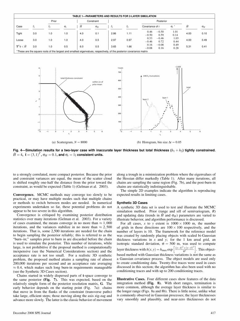
TABLE 1—PARAMETERS AND RESULTS FOR 2-LAYER SIMULATION

Prior Constraint Posterior

Case t1 t2 σt H σH t1 t2 Covariance of t σt∗ H σH

Tight 3.0 1.0 1.0 4.0 0.1 2.86 1.110.46 −0.50

−0.50 0.591.010.14 4.00 0.10

Loose 3.0 1.0 1.0 4.0 0.5 2.97 0.970.53 −0.46

−0.46 0.721.030.44 4.00 0.49

TT t < H 3.0 1.0 0.5 6.0 0.5 3.65 1.660.16 −0.08

−0.08 0.160.490.28 5.31 0.41

∗These are the square roots of the largest and smallest eigenvalues, respectively, of the posterior covariance matrix

−2 −1 0 1 2 3 4 5 6−2

−1

0

1

2

3

4

5

6

t1

t2

within 2σ ofprior mean

total thickness constraint

(a) Scattergram, N = 8000

−2 −1 0 1 2 3 4 5 60

100

200

300

400

500

600

700

t2

Counts~2,000

layer 2layer 1

total

648 h2-truncations

(b) Histogram, bin size ∆t = 0.05

Fig. 4—Simulation results for a two-layer case with inaccurate layer thickness but total thickness (h1 + h2) tightly constrained.H = 4, t = (3,1)T , σH = 0.1, and σt = 1; consistent units.

to a strongly correlated, more compact posterior. Because the priorand constraint variances are equal, the mean of the scatter cloudis shifted roughly one-half the distance from the prior toward theconstraint, as would be expected (Table 1) (Gelman et al. 2003).

Convergence. MCMC methods may converge too slowly to bepractical, or may have multiple modes such that multiple chainsor methods to switch between modes are needed. In numericalexperiments undertaken so far, these potential problems do notappear to be too severe in this algorithm.

Convergence is critiqued by examining posterior distributionstatistics over many iterations (Gelman et al. 2003). For a varietyof cases examined, the means converge in no more than ≈ 1,000iterations, and the variances stabilize in no more than ≈ 2,500iterations. That is, some 2,500 iterations are needed for the chainto begin sampling the posterior reliably; this is referred to as the“burn–in;” samples prior to burn in are discarded before the chainis used to simulate the posterior. This number of iterations, whilelarge, is not prohibitive if the proposal method is computationallyinexpensive (see the Numerical Considerations section) and theacceptance rate is not too small. For a realistic 3D syntheticproblem, the proposed method attains a sampling rate of almost200,000 iterations per second and an acceptance rate averaging≈ 0.4, which makes such long burn-in requirements manageable(see the Synthetic 3D Cases section).

Chains started in widely dispersed parts of t-space converge tothe same posterior (Fig. 7). This was expected, based on therelatively simple form of the posterior resolution matrix, G. Theearly behavior depends on the starting point (Fig. 7a): chainsthat move in from the flanks of the constraint (transverse paths)take large, efficient steps; those moving along the axis zig-zag andadvance more slowly. The latter is the classic behavior of movement

along a trough in a minimization problem where the eigenvalues ofthe Hessian differ markedly (Table 1). After many iterations, allchains are sampling the same region (Fig. 7b), and the post-burn-inchains are statistically indistinguishable.

The simple 2D examples indicate the algorithm is reproducingexpected results in limiting cases.

Synthetic 3D CasesA synthetic 3D data set is used to test and illustrate the MCMCsimulation method. Prior (range and sill of semivariogram, R)and updating data (trends in H and σH ) parameters are varied toillustrate behavior, and algorithm performance is discussed.

For all cases, x to y extent is 1000 × 1000 m, the numberof grids in those directions are 100 × 100 respectively, and thenumber of layers is 10. The framework for the reference modelwas created by randomly placing objects with scaled bi-Gaussianthickness variations in x and y; for the 1 km areal grid, anisotropic standard deviation, σ = 500 m, was used to compute

layer thickness with h(x,y)= hmax exp[

(x−x)2+(y−y)2

σ2

]. This object-

based method with Gaussian thickness variations is not the same asa Gaussian covariance process. The object models are used onlyto create conditioning data. Twenty-five traces were used in casesdiscussed in this section; the algorithm has also been used with noconditioning traces and with up to 200 conditioning traces.

Illustrative Cases. Four different cases show features of the dataintegration method (Fig. 8). With short ranges, termination ismore common, although the average layer thickness is similar tothe longer range (Figs. 8a and 8b). There is little noise, unlike whatis commonly observed in Gaussian processes; the layer thicknessesvary smoothly and plausibly, and near-zero thicknesses do not


−2 −1 0 1 2 3 4 5 6−2

−1

0

1

2

3

4

5

6

t1

t2




−2 −1 0 1 2 3 4 5 60

100

200

300

400

500

600

700

t2

Counts

layer 2

layer 1

total

1148 h2-truncations

(b) Histogram, bin size ∆t = 0.05

Fig. 5—Simulation results for a two-layer case with inaccurate layer and total thicknesses (h1 +h2). H = 4, t = (3,1)T , σH = 0.5,and σt = 1; consistent units.

appear in isolated areas; this results from the truncation rules andthe smooth Gaussian variogram. The pinchout pattern is clearer inthe longer-range case (Fig. 8b). In particular on the first cross-section in the left, the light layer near the base and the dark layerin the middle appear to taper and pinch out smoothly; this behavioris more characteristic of object models than most covariance-basedsimulations.

Seismic data may imply a thickness trend (Fig. 8c). Theseismic trend will be reproduced in the simulation, with a precisionconditioned on the inferred seismic thickness variance, σH . Ifthe seismic variance is higher for smaller mean thickness, lowthicknesses fluctuate more, as can be seen by comparing the leftfront edges of Figs. 8c and 8d. For the low variance case (Fig.8c), the edge panel is of nearly uniform thickness; the nonuniformvariance case (Fig. 8d) has much greater fluctuation on the left edge.

Although based on a synthetic case, these results indicate thatthe proposed method can reproduce complex pinchout layeringand plausible seismic trends. The number of pinchouts can bequite large in complex cornerpoint grids; 30,608 of 100,000 tracesegment are zero-thickness in one of the example cases (Fig.8c). The complex pinchout structure is obtained even though theconditioning data are not especially dense (Fig. 8d).

Performance. For adequate performance, an MCMC simulationshould converge to its target distribution in as few steps as possible.A large step size helps explore the posterior in few steps. Onthe other hand, large steps are more likely to be rejected, wastingcomputations on a sample that is not retained. The step sizeis usually adjusted indirectly, by scaling the posterior covariance(which is used to generate steps; see the Metropolis-Hastings Stepsubsection). For the system examined, the covariance is not scaled;this gives a step size of the order of the square root of the smallestdiagonal element in the posterior covariance matrix. In high-dimensional problems, it may be more appropriate to use Cπ =5.76

K Cπ to ensure adequate acceptance rates (Gelman et al. 2003).Although the unscaled covariance yields larger steps for K = 10, thetest cases had acceptance rates of 30 to 40 percent. This step sizeand acceptance rate appears to yield good convergence, thoroughexploration of the posterior, and smooth posterior samples (wherethey should be smooth: e.g., if the prior implies truncations are veryunlikely or almost certain). The best choice of scaling is problem-dependent.

The computational cost of a single simulation (for the case of

TABLE 2—PERFORMANCE SUMMARY FOR THE 3D EXAMPLE (ONECOMPLETE SIMULATION)∗

Process Work in Seconds∗∗

Kriging work 5.95Toeplitz solver work 0.22Total overhead all traces 6.17Samples, 5000 per trace, all traces 299.20Cost of example simulation, excluding io 305.37∗ model size, 100×100×10; 5,000 samples per trace∗∗ using a 2 GHz Pentium-M processor with 1 GB of RAM

Fig. 8a) is examined component-by-component in Table 2. Severalfeatures are striking. First, 97.98 percent of the work is donein the deepest part of the sampling loop, which requires randomnumber draws, extractions of submatrices, and multiplication ofrandom normal vectors by lower triangular matrices (the Choleskyfactor of the posterior covariance matrix, LCπκ). None of theseoperations is particularly expensive, but a total of 5×107 iterationswere performed for this case (≈ 164,000 samples accepted persecond). Because the kriging system is solved only once per trace—and is 2D, with an efficient k-d neighbor search—the associatedwork is small, about 1.95 percent. The Toeplitz manipulations arepractically cost-free, only about 0.07 percent of the total work.Finally, the overall cost of about 5 minutes on a laptop computer(for 105 unknowns) does not seem prohibitive.

Because it is a tracewise sequential algorithm, this MCMCmethod scales linearly in the number of block edges, or traces.Thus, a model with 106 traces and 10 layers should requireapproximately 8.5 hrs if attempted on a single Pentium-M processorwith adequate memory: not too alarming, for a model with 107

unknowns. The Toeplitz covariance and inversion work scalesapproximately with the third power of layer count (see the Numer-ical Considerations section), and linearly for generating samples attraces. However, Toeplitz solver work takes less than 1 percent ofthe computing time (Table 2). That is, although the cubic scaling isunfavorable for large K, the multiplier for the Toeplitz work is smalland this component does not control the total work required. Thisis because proposing samples consumes most of the work, and eachtrace has thousands of proposals and requires only one K3 Toeplitzsolve. The total, sampling-dominated work scales with K ratherthan K3. Therefore, a model with 20 layers takes approximatelytwice as long as the 10-layer model used in the illustrations.


−1 0 1 2 3 4 5 6−1

0

1

2

3

4

5

6

t1

t2




−1 0 1 2 3 4 5 6 70

100

200

300

400

500

600

700

t2

Counts

layer 2

layer 1

total

(b) Histogram, bin size ∆h = 0.05

Fig. 6—Simulation results for a two-layer case with prior sum less than the sum constraint. H = 6, t = (3,1)T , σH = 0.5, andσt = 0.5; consistent units.

DiscussionSequential Methods. A difficult aspect of these nonlinear down-scaling problems is discerning whether the overall system posteriordistribution can be safely factored into the product of conditionaldistributions implied by the sequential pass over the columns ofgridblocks. This factorization requires computing both analyti-cal marginal distributions (integrating over unvisited sites), andconditional distributions dependent only on visited sites. Thisrequirement is usually met only by exponential family distributionfunctions. The posterior in our problem does not strictly satisfythese requirements. Nonetheless, the approximations we make candoubtless be improved by blockwise sequential schemes, thougha block approach increases both the dimensionality of the MCMCsampling subproblem and the configurational complexity of han-dling more pinchout transitions.

Notwithstanding these concerns, we have demonstrated thatusing auxiliary variables greatly facilitates effective sampling ofa complicated high-dimensional posterior distribution that arisesin the downscaling problem we address. Similar difficulties willarise in any more or less rigorous recasting of the problem, so thetechnique we demonstrate should be widely applicable. Possibleextensions are use of mixture-independence samplers (Gilks et al.1996) that take advantage of the piecewise quadratic form of thelog-posterior function, and generalization to multiple correlatedvariables in the model and associated likelihood.

Related Methods. As discussed in Simulation of Two-Layer Sys-tems, if no layers are likely to be absent, the posterior distributionremains multi-Gaussian, and simulation and estimation methods arelinear. In this case, the proposed method is a variant of collocatedcokriging, where the collocated data are a sum rather than aconstraint on a single thickness (Goovaerts 1997). The proposedmethods are needed only when there is substantial likelihood oflayers terminating laterally, in which case untruncated Gaussianmodels will fail.

Previous work on reservoir characterization with truncated Gaus-sian fields has focused on categorical simulations (Xu and Journel1993; Matheron et al. 1987). In contrast, the proposed methodcombines aspects of categorical and continuous simulations. Thecondition tk ≤ 0 on the thickness proxy is equivalent to setting anindicator for layer occurrence to zero. However, in the categoricalcase all tk > 0 would be identical (for a binary case), whereas weuse values tk > 0 to model the continuous variable hk. This hybrid

approach could be applied without constraints, yielding sequen-tial truncated Gaussian simulations of thickness; this correspondsclosely to the cases with high σH presented above, and the resultingimages would be similar.

Cornerpoint Grids. The MCMC simulation is over the blockedges, or traces. This is different from many geostatistical mod-eling approaches, which are commonly block-centered. However,geometry—especially pinchouts or discontinuities at faults—canbe modeled more accurately using cornerpoints. The porosityand other rock properties should be simulated or estimated atthe same point, because these properties are generally correlatedthrough the rock physics model and seismic response. Even forcornerpoint grids, reservoir simulators use block centered valuesfor rock properties such as porosity. The trace properties mustbe averaged appropriately to the block center. A simple mean isprobably adequate for thickness and porosity-thickness. However,the permeability must be upscaled more carefully, especially fornonrectangular blocks; a good method might be to integrate theJacobian over the half-block domains (Peaceman 1996). Even foruniform permeability, the Jacobian integration correctly providesface- and direction-dependent transmissibilities for a nonrectangu-lar grid. The method could also be used to perform approximateupscaling for sublayer heterogeneities and compute more accuratepore and bulk volumes.

Extensions. Three extensions are discussed in other, related work.First, several distinct facies are subjected to separate seismic thick-ness constraints (Kalla et al. 2007b). This permits, for example,conditioning on net and gross thickness separately. Second, productconstraints, of the form ∑

Kk=1 hkφk = ΦH, can be imposed; these

constraints are nonlinear (Kalla et al. 2007b). More general scalelinkages have been implemented using Markov random fields (Leeet al. 2002). Third, block methods or other approaches wereconsidered by Kalla et al. (2007a) to address difficulties with thecomputation of marginal distributions in non-Gaussian sequentialsimulation (see the Sequential Methods subsection).

ConclusionsStochastic seismic inversion computations can be integrated with atruncated Gaussian geostatistical model for layer thicknesses usingan MCMC method. Truncation makes the problem nonlinear,which is ameliorated by the introduction of auxiliary variables and


0 1 2 3 4 5 6−2

−1

0

1

2

3

4

t1

t2

starting points

chains of accepted proposals

transversepath

axial path

(a) First 150 samples of four chains

0 1 2 3 4 5 6−2

−1

0

1

2

3

4

t1

t2

(b) Converging chains with 10,000 samples per chain

Fig. 7—Four Markov chains starting from diverse points tend to migrate toward the most likely region. (a) Convergence is slowerfor points that must move along the axis to reach the area of the mode. (b) Results are practically identical for long chains,because the posterior is unimodal. The prior and constraint data are the same as in Fig. 4.

a mixed Gibbs-Metropolis-Hastings sampling procedure. Underreasonable assumptions, the posterior resolution matrix is a specialform of Toeplitz matrix; the special form can be exploited to makeMCMC sample proposals more efficient to evaluate. Proposalefficiency is critical to the usefulness of the method, because manythousands of proposals must be evaluated at each trace for a singlecornerpoint grid realization. The ability of the method to reproducelimiting case results and correctly model truncations is verifiedby examining algorithm behavior in two dimensions. A synthetic3D case demonstrates that the procedure is acceptably fast. Al-though many issues remain—especially implementation of morecomplex constraints and integration with fine-scale geomodels—the proposed method appears to offer a foundation for furtherdevelopment.

AcknowledgmentsBHP-Billiton funded this research by research agreements andan unrestricted gift to Louisiana State University, and researchagreements with CSIRO. The authors are grateful for this support,and for permission to publish this paper. Schlumberger providedaccess to Petrel reservoir modeling software, used for visualizationin this research. Two anonymous reviewers provided insightful,detailed corrections and suggestions, which have improved thepaper significantly.

NomenclatureCp = prior covariance matrix based on kriging, m2

Cπ = posterior covariance matrix, m2

G = posterior resolution matrix or Hessian, m−2

d = neighboring conditioningh = nonnegative layer thickness, mH = total thickness at trace, mL = Cholesky factor of covariance matrix, mN(µ,σ2) = normal distribution function with mean µ and

variance σ2

N−1(µ,σ2;r) = inverse normal distribution function with meanµ and variance σ2, at a cumulative probability ofr

p = probability densityP = probabilityr = random numberRx = covariance range parameter in direction x, m

s = scaling factort = Gaussian proxy for h, may be negative, mu = auxiliary variable correlated to layer stateU = uniform distribution functionT = Tk = 1

2 (sgn(tk)+1)W = computational work, flopsx,y,z = coordinates, mX ,Y,Z = grid extents, mα = Metropolis-Hastings transition probabilityγ = semivariogram model∆ = separation vector for variogram models, mφ = layer porosityΦ = trace average porosityκ = number of layers at a trace with tk > 0π = posteriorσ2 = variance

Indices and Special SubscriptsD = number of nonzero conditioning datak = indices over layersK = total number of layers` = indices over tracesL = total number of tracesp = priorλ,Λ = zero thickness data index and count

Diacritical Marks· = mean·′ = proposed point, may become new point

ReferencesBehrens, R.A., MacLeod, M.K., and Tran, T.T., 1998. Incorpo-

rating seismic attribute maps in 3d reservoir models. SPEREE,1 (2): 122–126. SPE-36499-PA. DOI: 10.2118/36499-PA.

Bentley, J.L., 1975. Multidimensional binary search trees usedfor associative searching. Communications of the ACM, 18 (9):509–517.

Deutsch, C.V. and Journel, A.G., 1998. GLSIB: GeostatisticalSoftware Library and User’s Guide. New York: AppliedGeostatistics Series. Oxford University Press, Oxford, New


(a) Short range, R = 200 (b) Long range, R = 750

(c) Seismic thickness trend, H = 7 + 13xX , R = 350; x = 0 is on the left

front(d) Noise varies, σH = 5− 3x

X ; R and H as in (c); x = 0 is on the left front

Fig. 8—Simulations on 100 × 100 × 10 cornerpoint grids, areal extent is X = Y = 1000 m, and 25 conditioning traces areused. Unless otherwise noted, H = 20 and σH = 2. All realizations use a Gaussian semivariogram with Rx = Ry = R, γ(∆) =

1− exp[−(||∆||/R)2

], m2. All models flattened on the topmost surface. Range, thickness, and standard deviation are in m. 7.5×

vertical exaggeration for all figures. Vertical black lines in (d) are conditioning traces.

York, second edition.

Deutsch, C.V., Srinivasan, S., and Mo, Y., 1996. Geostatisticalreservoir modeling accounting for precision and scale of seismicdata. Paper SPE 36497 presented at SPE Annual TechnicalConference and Exhibition, Dallas, Texas, 6-9 October. DOI:10.2118/36497-MS.

Dobrin, M.B. and Savit, C.H., 1988. Introduction to GeophysicalProspecting. McGraw-Hill, New York, fourth edition.

Doyen, P.M., Psaila, D.E., den Boer, L.D., and Jans, D., 1997.Reconciling data at seismic and well log scales in 3-d earthmodeling. Paper SPE 38698 presented at SPE Annual TechnicalConference and Exhibition, San Antonio, Texas, 5-8 October.DOI: 10.2118/38698-MS.

Eclipse 100 Reference Manual. 2004. Schlumberger TechnologyCo., Oxfordshire, UK.

Gelman, A., Carlin, J.B., Stern, H.S., and Rubin, D.B., 2003.Bayesian Data Analysis. CRC Press, Boca Raton, Florida,second edition.

Gilks, W.R., Richardson, S., and Spiegelhalter, D.J., 1996. MarkovChain Monte Carlo in Practice. Chapman and Hall, London.

Glinsky, M.E., Asher, B., Hill, R., Flynn, M., Stanley, M.,Gunning, J., Thompson, T., et al., 2005. Integrationof uncertain subsurface information into multiple reservoirsimulation models. The Leading Edge, 24 (10): 990–999. DOI:10.1190/1.2112372.

Golub, G.H. and van Loan, C.F., 1996. Matrix Computations.Johns Hopkins University Press, Baltimore, Maryland, thirdedition.

Goovaerts, P., 1997. Geostatistics for Natural ResourcesEvaluation. Applied Geostatistics Series. Oxford UniversityPress, Oxford, New York.

Gunning, J.G. and Glinsky, M.E., 2004. Delivery: Anopen-source model-based Bayesian seismic inversion program.Computers & Geosciences, 30 (6): 619–636. DOI:10.1016/j.cageo.2003.10.013.

Gunning, J.G. and Glinsky, M.E., 2006. Wavelet ex-tractor: A Bayesian well-tie wavelet derivation program.


Computers & Geosciences, 32 (5): 681–695. DOI:10.1016/j.cageo.2005.10.001.

Gunning, J.G., Glinsky, M.E., and White, C.D., 2007. Deliverymassager: A tool for propagating seismic inversion informationinto reservoir models. Computers & Geosciences, 33 (5): 630–648. DOI: 10.1016/j.cageo.2006.09.004.

Higdon, D.M., 1998. Auxiliary variable methods for Markovchain Monte Carlo with applications. Journal of theAmerican Statistical Association, 93 (442): 585–595. DOI:10.2307/2670110.

Kalla, S., White, C.D., and Gunning, J., 2007a. Downscalingseismic data to the meter scale: Sampling and marginalization.EAGE, Presented at Petroleum Geostaistics, Cascais, Portugal,10-14 September.

Kalla, S., White, C.D., Gunning, J., and Glinsky, M.E., 2007b.Imposing multiple seismic inversion constraints on reservoirsimulation models using block and sequential methods. PaperSPE 110771 presented at SPE Annual Technical Conferenceand Exhibition, Anaheim, California, 11-14 November. DOI:10.2118/110771-MS.

Lee, S.H., Malallah, A., Datta-Gupta, A., and Higdon, D.M.,2002. Multiscale data integration using markov random fields.SPEREE, 5 (1): 68–78. SPE-76905-PA. DOI: 10.2118/76905-PA.

Matheron, G., Beucher, H., de Fouquet, C., and Galli, A.,1987. Conditional simulation of the geometry of fluvio-deltaicreservoirs. Paper SPE 16753 presented at SPE Annual TechnicalConference and Exhibition, Dallas, Texas, 27-30 September.DOI: 10.2118/16753-MS.

Merriam, D.F. and Davis, J.C. (eds.), 2001. Sedsim in HydrocarbonExploration, 71–97. Kluwer Academic+Plenum Publishers,New York.

Nocedal, J. and Wright, S.J., 1999. Numerical Optimization.Springer Science+Business Media, New York.

Peaceman, D.W., 1996. Calculation of transmissibilities of grid-blocks defined by arbitrary cornerpoint geometry. Richardson,Texas. Paper SPE 37306 available from SPE.

Petrel Workflow Tools, Introduction Course. 2005. SchlumbergerTechnology Co., Oslo, Norway.

Ponting, D.K., 1989. Corner point grid geometry in reservoirsimulation. Proc., Joint IMA/SPE European Conference on theMathematics of Oil Recovery, Cambridge, UK.

Pyrcz, M.J., 2004. The Integration of Geologic Information intoGeostatistical Models. Ph.D. thesis, University of Alberta,Edmonton, Alberta, Canada.

Widess, M.B., 1973. How thin is a thin bed? Geophysics, 38 (6):1176–1180. DOI: 10.1190/1.1440403.

Willis, B.J. and White, C.D., 2000. Quantitative outcropdata for flow simulation. Journal of Sedimentary Research,70 (4): 788–802. DOI: 10.1306/2DC40938-0E47-11D7-8643000102C1865D.

Xu, W. and Journel, A.G., 1993. GTSIM: Gaussian truncatedsimulations of reservoir units in a W. Texas carbonate field.Richardson, Texas. Paper SPE 27412 available from SPE.

Appendix—Zero Thickness Conditioning DataIn this paper, the untruncated Gaussian proxy t is kriged, not theactual thickness h. At simulated traces, t is computed and stored,and only converted to h for output. Conditioning data present moreof a challenge. If we observe some layer k on trace ` has h`k =0, the value of t`k is indeterminate; we only know t`k ≤ 0. Theconditioning data might be decorrelated if we used a simple butreasonable draw such as

tk = N−1(

tk,σ2tk;r)

,r ∼U [0,P(hk = 0)], . . . . . . . . . (A1)

where P(hk = 0) is given by Eq. 1, N is normal distributionfunction, and U is the uniform distribution function. Instead, wemodel the correlation as follows, with a loop over all layers.

• Find all zero conditioning data in this layer, k; the list of thelocations of zero data is indexed over λk ∈ {0 . . .Λk}. The positiveconditioning data in layer k are indexed by d ∈ {0 . . .Dk}.

• Initialize all Λk zero thickness observations in layer k withrandom draws, using Eq. A1.

• Visit each point λ, forming a kriging system of size Dk +Λk−1, composed of all points in this layer except the current point.Compute the mean and variance, and draw r ∼U [0,P(hk = 0)]; inthe first iteration, the kriging weights and variances are stored forreuse. P(hk = 0) is computed using the new mean and standarddeviation of tk. The new simulated value tk is the inverse ofN(tk,σ2

tk) at cumulative probability r.• Generate a chain and store.• Repeat ∀k ∈ {1 . . .K}

The stored chains can be used at the beginning in later simulationsof layer thickness. Before simulating any new points, sets of thezero-thickness conditioning data are drawn from the stored chain.

Subhash Kalla is a PhD student in petroleum engineering atLouisiana State University. email: [email protected]. He holdsan MS degree in petroleum engineering from Louisiana StateUniversity. and a BTech degree in chemical engineering fromthe Regional Engineering College (now National Institute ofTechnology), Warangal, India. His research interests includereservoir simulation, reservoir characterization, and uncertaintyanalysis. Christopher D. White is an associate professor ofpetroleum engineering at Louisiana State University. He holdsa BS degree from the University of Oklahoma and MS and PhDdegrees from Stanford University, all in petroleum engineering.email: [email protected]. Formerly, White was a researchengineer for Shell Development Company and a researchscientist for the Bureau of Economic Geology, the Universityof Texas at Austin. His research interests include general reser-voir engineering, reservoir simulation, and statistics. JamesGunning is senior research scientist in the CSIRO petroleumreservoir characterisation area. He holds a BS degree inphysics, a BEE degree in electrical engineering, and a PhDdegree in applied mathematics, all from Melbourne University.His current research interests are in spatial statistics, Bayesianmethodologies, uncertainty quantification, data integration,and inverse problems from remote sensing tools like seismic andelectromagnetic methods. Michael E. Glinsky is the SectionLeader of Quantitative Interpretation for BHP Billiton Petroleum.He holds a BS degree in physics from Case Western ReserveUniversity and a PhD degree in physics from the University ofCalifornia, San Diego. He worked as a Department of EnergyDistinguished Postdoctoral Research Fellow at Lawrence Liver-more National Laboratory for five years. He worked for threeyears at the Shell E&P Technology Co. researching on BayesianAVO and 4D inversion. He has published more than 25 papersin the scientific literature on subjects as varied as plasmaphysics, signal processing for oil exploration, x-ray diagnostics,application of exterior calculus to theoretical mechanics, andlaser biological tissue interactions.


consistent downscaling of seismic inversion thicknesses to ... · thickness are general, and need...

Documents