Consistent Kernel Mean Estimationfor Functions of Random Variables

Carl-Johann Simon-Gabriel∗, Adam Scibior∗,†, Ilya Tolstikhin, Bernhard SchölkopfDepartment of Empirical Inference, Max Planck Institute for Intelligent Systems

Spemanstraße 38, 72076 Tübingen, Germany∗ joint first authors; † also with: Engineering Department, Cambridge University

cjsimon@, adam.scibior@, ilya@, bs@tuebingen.mpg.de

Abstract

We provide a theoretical foundation for non-parametric estimation of functions ofrandom variables using kernel mean embeddings. We show that for any continuousfunction f , consistent estimators of the mean embedding of a random variable Xlead to consistent estimators of the mean embedding of f(X). For Matérn kernelsand sufficiently smooth functions we also provide rates of convergence.Our results extend to functions of multiple random variables. If the variablesare dependent, we require an estimator of the mean embedding of their jointdistribution as a starting point; if they are independent, it is sufficient to haveseparate estimators of the mean embeddings of their marginal distributions. Ineither case, our results cover both mean embeddings based on i.i.d. samples as wellas “reduced set” expansions in terms of dependent expansion points. The latterserves as a justification for using such expansions to limit memory resources whenapplying the approach as a basis for probabilistic programming.

1 Introduction

A common task in probabilistic modelling is to compute the distribution of f(X), given a measurablefunction f and a random variable X . In fact, the earliest instances of this problem date back at leastto Poisson (1837). Sometimes this can be done analytically. For example, if f is linear and X isGaussian, that is f(x) = ax+ b and X ∼ N (µ;σ), we have f(X) ∼ N (aµ+ b; aσ). There existvarious methods for obtaining such analytical expressions (Mathai, 1973), but outside a small subsetof distributions and functions the formulae are either not available or too complicated to be practical.

An alternative to the analytical approach is numerical approximation, ideally implemented as aflexible software library. The need for such tools is recognised in the general programming languagescommunity (McKinley, 2016), but no standards were established so far. The main challenge is infinding a good approximate representation for random variables.

Distributions on integers, for example, are usually represented as lists of (xi, p(xi)) pairs. For realvalued distributions, integral transforms (Springer, 1979), mixtures of Gaussians (Milios, 2009), La-guerre polynomials (Williamson, 1989), and Chebyshev polynomials (Korzen and Jaroszewicz, 2014)were proposed as convenient representations for numerical computation. For strings, probabilisticfinite automata are often used. All those approaches have their merits, but they only work with aspecific input type.

There is an alternative, based on Monte Carlo sampling (Kalos and Whitlock, 2008), which is torepresent X by a (possibly weighted) sample {(xi, wi)}ni=1 (with wi ≥ 0). This representation hasseveral advantages: (i) it works for any input type, (ii) the sample size controls the time-accuracytrade-off, and (iii) applying functions to random variables reduces to applying the functions pointwise

30th Conference on Neural Information Processing Systems (NIPS 2016), Barcelona, Spain.

to the sample, i.e., {(f(xi), wi)} represents f(X). Furthermore, expectations of functions of randomvariables can be estimated as E [f(X)] ≈

∑i wif(xi)/

∑i wi, sometimes with guarantees for the

convergence rate.

The flexibility of this Monte Carlo approach comes at a cost: without further assumptions on theunderlying input space X , it is hard to quantify the accuracy of this representation. For instance,given two samples of the same size, {(xi, wi)}ni=1 and {(x′i, w′i)}ni=1, how can we tell which one is abetter representation of X? More generally, how could we optimize a representation with predefinedsample size?

There exists an alternative to the Monte Carlo approach, called Kernel Mean Embeddings (KME)(Berlinet and Thomas-Agnan, 2004; Smola et al., 2007). It also represents random variables assamples, but additionally defines a notion of similarity between sample points. As a result, (i) itkeeps all the advantages of the Monte Carlo scheme, (ii) it includes the Monte Carlo method asa special case, (iii) it overcomes its pitfalls described above, and (iv) it can be tailored to focuson different properties of X , depending on the user’s needs and prior assumptions. The KMEapproach identifies both sample points and distributions with functions in an abstract Hilbert space.Internally the latter are still represented as weighted samples, but the weights can be negative andthe straightforward Monte Carlo interpretation is no longer valid. Schölkopf et al. (2015) proposeusing KMEs as approximate representation of random variables for the purpose of computing theirfunctions. However, they only provide theoretical justification for it in rather idealised settings, whichdo not meet practical implementation requirements.

In this paper, we build on this work and provide general theoretical guarantees for the proposed esti-mators. Specifically, we prove statements of the form “if {(xi, wi)}ni=1 provides a good estimate forthe KME of X , then {(f(xi), wi)}ni=1 provides a good estimate for the KME of f(X)”. Importantly,our results do not assume joint independence of the observations xi (and weights wi). This makesthem a powerful tool. For instance, imagine we are given data {(xi, wi)}ni=1 from a random variableX that we need to compress. Then our theorems guarantee that, whatever compression algorithm weuse, as long as the compressed representation {(x′j , w′j)}nj=1 still provides a good estimate for theKME of X , the pointwise images {(f(x′j), w

′j)}nj=1 provide good estimates of the KME of f(X).

In the remainder of this section we first introduce KMEs and discuss their merits. Then we explainwhy and how we extend the results of Schölkopf et al. (2015). Section 2 contains our main results. InSection 2.1 we show consistency of the relevant estimator in a general setting, and in Section 2.2 weprovide finite sample guarantees when Matérn kernels are used. In Section 3 we show how our resultsapply to functions of multiple variables, both interdependent and independent. Section 4 concludeswith a discussion.

1.1 Background on kernel mean embeddings

Let X be a measurable input space. We use a positive definite bounded and measurable kernelk : X × X → R to represent random variables X ∼ P and weighted samples X := {(xi, wi)}ni=1

as two functions µkX and µkX in the corresponding Reproducing Kernel Hilbert Space (RKHS)Hk bydefining

µkX :=

∫k(x, .) dP (x) and µkX :=

∑i

wik(xi, .) .

These are guaranteed to exist, since we assume the kernel is bounded (Smola et al., 2007). Whenclear from the context, we omit the kernel k in the superscript. µX is called the KME of P , but wealso refer to it as the KME of X . In this paper we focus on computing functions of random variables.For f : X → Z , where Z is a measurable space, and for a positive definite bounded kz : Z ×Z → Rwe also write

µkzf(X) :=

∫kz(f(x), .) dP (x) and µkzf(X) :=

∑i

wikz(f(xi), .) . (1)

The advantage of mapping random variables X and samples X to functions in the RKHS is thatwe may now say that X is a good approximation for X if the RKHS distance ‖µX − µX‖ issmall. This distance depends on the choice of the kernel and different kernels emphasise differentinformation about X . For example if on X := [a, b] ⊂ R we choose k(x, x′) := x · x′ + 1, then

2

µX(x) = EX∼P [X]x+ 1. Thus any two distributions and/or samples with equal means are mappedto the same function inHk so the distance between them is zero. Therefore using this particular k,we keep track only of the mean of the distributions. If instead we prefer to keep track of all firstp moments, we may use the kernel k(x, x′) := (x · x′ + 1)p. And if we do not want to loose anyinformation at all, we should choose k such that µk is injective over all probability measures on X .Such kernels are called characteristic. For standard spaces, such as X = Rd, many widely usedkernels were proven characteristic, such as Gaussian, Laplacian, and Matérn kernels (Sriperumbuduret al., 2010, 2011).

The Gaussian kernel k(x, x′) := e−‖x−x′‖2

2σ2 may serve as another good illustration of the flexibilityof this representation. Whatever positive bandwidth σ2 > 0, we do not lose any information aboutdistributions, because k is characteristic. Nevertheless, if σ2 grows, all distributions start looking thesame, because their embeddings converge to a constant function 1. If, on the other hand, σ2 becomessmall, distributions look increasingly different and µX becomes a function with bumps of height wiat every xi. In the limit when σ2 goes to zero, each point is only similar to itself, so µX reduces tothe Monte Carlo method. Choosing σ2 can be interpreted as controlling the degree of smoothing inthe approximation.

1.2 Reduced set methods

An attractive feature when using KME estimators is the ability to reduce the number of ex-pansion points (i.e., the size of the weighted sample) in a principled way. Specifically, ifX ′ := {(x′j , 1/N)}Nj=1 then the objective is to construct X := {(xi, wi)}ni=1 that minimises‖µX′ − µX‖ with n < N . Often the resulting xi are mutually dependent and the wi certainlydepend on them. The algorithms for constructing such expansions are known as reduced set methodsand have been studied by the machine learning community (Schölkopf and Smola, 2002, Chapter 18).

Although reduced set methods provide significant efficiency gains, their application raises certainconcerns when it comes to computing functions of random variables. Let P,Q be distributions of Xand f(X) respectively. If x′j ∼i.i.d. P , then f(x′j) ∼i.i.d. Q and so µf(X′) = 1

N

∑j k(f(x′j), .)

reduces to the commonly used√N -consistent empirical estimator of µf(X) (Smola et al., 2007).

Unfortunately, this is not the case after applying reduced set methods, and it is not known underwhich conditions µf(X) is a consistent estimator for µf(X).

Schölkopf et al. (2015) advocate the use of reduced expansion set methods to save computationalresources. They also provide some reasoning why this should be the right thing to do for characteristickernels, but as they state themselves, their rigorous analysis does not cover practical reduced setmethods. Motivated by this and other concerns listed in Section 1.4, we provide a generalised analysisof the estimator µf(X), where we do not make assumptions on how xi and wi were generated.

Before doing that, however, we first illustrate how the need for reduced set methods naturally emergeson a concrete problem.

1.3 Illustration with functions of two random variables

Suppose that we want to estimate µf(X,Y ) given i.i.d. samples X ′ = {x′i, 1/N}Ni=1 and Y ′ =

{y′j , 1/N}Nj=1 from two independent random variables X ∈ X and Y ∈ Y respectively. Let Q bethe distribution of Z = f(X,Y ).

The first option is to consider what we will call the diagonal estimator µ1 := 1N

∑ni=1 kz

(f(x′i, y

′i), .).

Since f(x′i, y′i) ∼i.i.d. Q, µ1 is

√N -consistent (Smola et al., 2007). Another option is to con-

sider the U-statistic estimator µ2 := 1N2

∑Ni,j=1 kz

(f(x′i, y

′j), .), which is also known to be

√N -

consistent. Experiments show that µ2 is more accurate and has lower variance than µ1 (see Figure 1).However, the U-statistic estimator µ2 needs O(n2) memory rather than O(n). For this reasonSchölkopf et al. (2015) propose to use a reduced set method both on X ′ and Y ′ to get new sam-ples X = {xi, wi}ni=1 and Y = {yj , uj}nj=1 of size n � N , and then estimate µf(X,Y ) usingµ3 :=

∑ni,j=1 wiujkx(f(xi, yj), .).

3

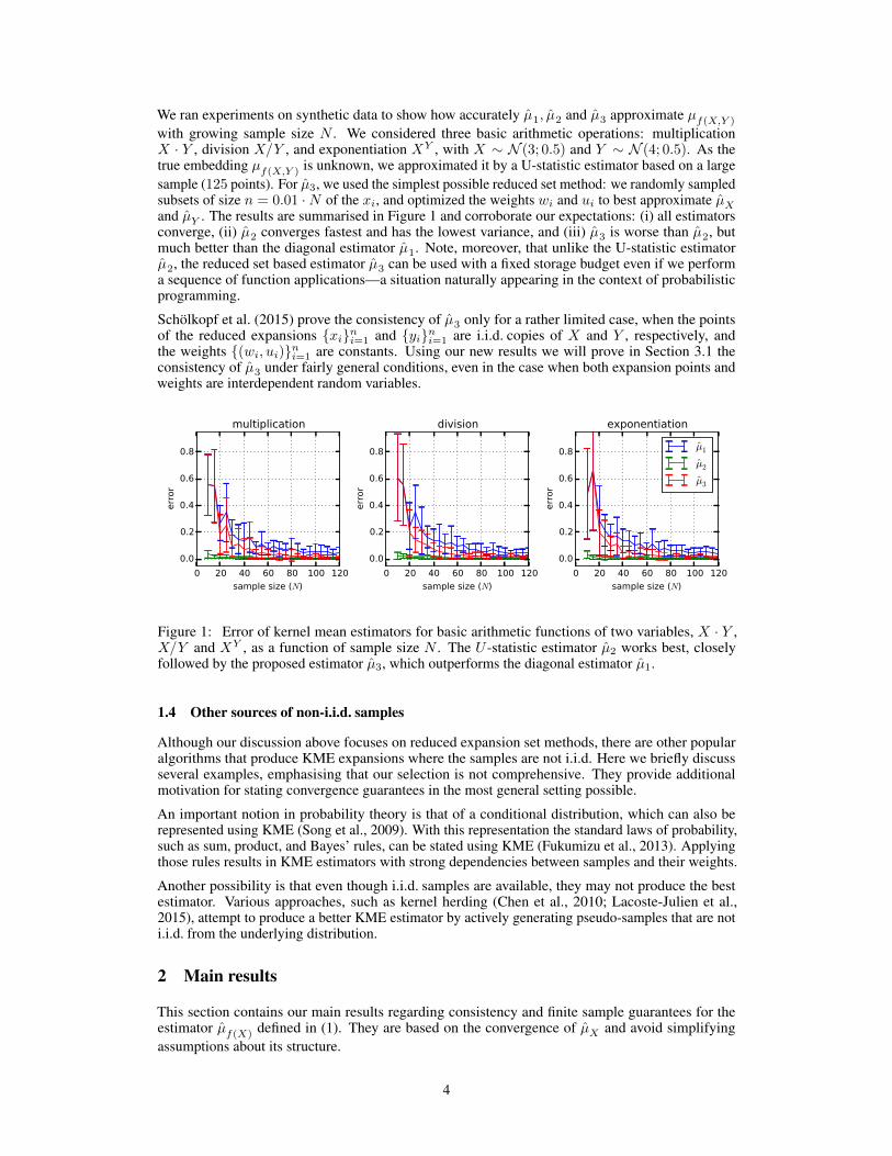
We ran experiments on synthetic data to show how accurately µ1, µ2 and µ3 approximate µf(X,Y )

with growing sample size N . We considered three basic arithmetic operations: multiplicationX · Y , division X/Y , and exponentiation XY , with X ∼ N (3; 0.5) and Y ∼ N (4; 0.5). As thetrue embedding µf(X,Y ) is unknown, we approximated it by a U-statistic estimator based on a largesample (125 points). For µ3, we used the simplest possible reduced set method: we randomly sampledsubsets of size n = 0.01 ·N of the xi, and optimized the weights wi and ui to best approximate µXand µY . The results are summarised in Figure 1 and corroborate our expectations: (i) all estimatorsconverge, (ii) µ2 converges fastest and has the lowest variance, and (iii) µ3 is worse than µ2, butmuch better than the diagonal estimator µ1. Note, moreover, that unlike the U-statistic estimatorµ2, the reduced set based estimator µ3 can be used with a fixed storage budget even if we performa sequence of function applications—a situation naturally appearing in the context of probabilisticprogramming.

Schölkopf et al. (2015) prove the consistency of µ3 only for a rather limited case, when the pointsof the reduced expansions {xi}ni=1 and {yi}ni=1 are i.i.d. copies of X and Y , respectively, andthe weights {(wi, ui)}ni=1 are constants. Using our new results we will prove in Section 3.1 theconsistency of µ3 under fairly general conditions, even in the case when both expansion points andweights are interdependent random variables.

0 20 40 60 80 100 120

sample size (N)

0.0

0.2

0.4

0.6

0.8

err

or

multiplication

0 20 40 60 80 100 120

sample size (N)

0.0

0.2

0.4

0.6

0.8

err

or

division

0 20 40 60 80 100 120

sample size (N)

0.0

0.2

0.4

0.6

0.8

err

or

exponentiation

µ1

µ2

µ3

Figure 1: Error of kernel mean estimators for basic arithmetic functions of two variables, X · Y ,X/Y and XY , as a function of sample size N . The U -statistic estimator µ2 works best, closelyfollowed by the proposed estimator µ3, which outperforms the diagonal estimator µ1.

1.4 Other sources of non-i.i.d. samples

Although our discussion above focuses on reduced expansion set methods, there are other popularalgorithms that produce KME expansions where the samples are not i.i.d. Here we briefly discussseveral examples, emphasising that our selection is not comprehensive. They provide additionalmotivation for stating convergence guarantees in the most general setting possible.

An important notion in probability theory is that of a conditional distribution, which can also berepresented using KME (Song et al., 2009). With this representation the standard laws of probability,such as sum, product, and Bayes’ rules, can be stated using KME (Fukumizu et al., 2013). Applyingthose rules results in KME estimators with strong dependencies between samples and their weights.

Another possibility is that even though i.i.d. samples are available, they may not produce the bestestimator. Various approaches, such as kernel herding (Chen et al., 2010; Lacoste-Julien et al.,2015), attempt to produce a better KME estimator by actively generating pseudo-samples that are noti.i.d. from the underlying distribution.

2 Main results

This section contains our main results regarding consistency and finite sample guarantees for theestimator µf(X) defined in (1). They are based on the convergence of µX and avoid simplifyingassumptions about its structure.

4

2.1 Consistency

If kx is c0-universal (see Sriperumbudur et al. (2011)), consistency of µf(X) can be shown in a rathergeneral setting.Theorem 1. Let X and Z be compact Hausdorff spaces equipped with their Borel σ-algebras,f : X → Z a continuous function, kx, kz continuous kernels on X ,Z respectively. Assume kx isc0-universal and that there exists C such that

∑i |wi| ≤ C independently of n. The following holds:

If µkxX → µkxX then µkzf(X) → µkzf(X) as n→∞.

Proof. Let P be the distribution of X and Pn =∑ni=1 wiδxi . Define a new kernel on X by

kx(x1, x2) := kz(f(x1), f(x2)

). X is compact and {Pn |n ∈ N} ∪ {P} is a bounded set (in

total variation norm) of finite measures, because ‖Pn‖TV =∑ni=1 |wi| ≤ C. Furthermore, kx

is continuous and c0-universal. Using Corollary 52 of Simon-Gabriel and Schölkopf (2016) weconclude that: µkxX → µkxX implies that P converges weakly to P . Now, kz and f being continuous,

so is kx. Thus, if P converges weakly to P , then µkxX → µkxX (Simon-Gabriel and Schölkopf, 2016,

Theorem 44, Points (1) and (iii)). Overall, µkxX → µkxX implies µkxX → µkxX . We conclude the proofby showing that convergence inHkx leads to convergence inHkz :∥∥∥µkzf(X) − µ

kzf(X)

∥∥∥2kz

=∥∥∥µkxX − µkxX ∥∥∥2

kx→ 0.

For a detailed version of the above, see Appendix A.

The continuity assumption is rather unrestrictive. All kernels and functions defined on a discretespace are continuous with respect to the discrete topology, so the theorem applies in this case. ForX = Rd, many kernels used in practice are continuous, including Gaussian, Laplacian, Matérn andother radial kernels. The slightly limiting factor of this theorem is that kx must be c0-universal, whichoften can be tricky to verify. However, most standard kernels—including all radial, non-constantkernels—are c0-universal (see Sriperumbudur et al., 2011). The assumption that the input domainis compact is satisfied in most applications, since any measurements coming from physical sensorsare contained in a bounded range. Finally, the assumption that

∑i |wi| ≤ C can be enforced, for

instance, by applying a suitable regularization in reduced set methods.

2.2 Finite sample guarantees

Theorem 1 guarantees that the estimator µf(X) converges to µf(X) when µX converges to µX .However, it says nothing about the speed of convergence. In this section we provide a convergencerate when working with Matérn kernels, which are of the form

ksx(x, x′) =21−s

Γ(s)‖x− x′‖s−d/22 Bd/2−s (‖x− x′‖2) , (2)

where Bα is a modified Bessel function of the third kind (also known as Macdonald function) oforder α, Γ is the Gamma function and s > d

2 is a smoothness parameter. The RKHS induced byksx is the Sobolev spaceW s

2 (Rd) (Wendland, 2004, Theorem 6.13 & Chap.10) containing s-timesdifferentiable functions. The finite-sample bound of Theorem 2 is based on the analysis of Kanagawaet al. (2016), which requires the following assumptions:

Assumptions 1. Let X be a random variable over X = Rd with distribution P and let X ={(xi, wi)}ni=1 be random variables over Xn×Rn with joint distribution S. There exists a probabilitydistribution Q with full support on Rd and a bounded density, satisfying the following properties:

(i) P has a bounded density function w.r.t. Q;(ii) there is a constant D > 0 independent of n, such that

ES

[1

n

n∑i=1

g2(xi)

]≤ D ‖g‖2L2(Q) , ∀g ∈ L2(Q) .

5

These assumptions were shown to be fairly general and we refer to Kanagawa et al. (2016, Section4.1) for various examples where they are met. Next we state the main result of this section.

Theorem 2. LetX = Rd, Z = Rd′ , and f : X → Z be an α-times differentiable function (α ∈ N+).Take s1 > d/2 and s2 > d′ such that s1, s2/2 ∈ N+. Let ks1x and ks2z be Matérn kernels over X andZ respectively as defined in (2). Assume X ∼ P and X = {(xi, wi)}ni=1 ∼ S satisfy 1. Moreover,assume that P and the marginals of x1, . . . xn have a common compact support. Suppose that, forsome constants b > 0 and 0 < c ≤ 1/2:

(i) ES[‖µX − µX‖

2ks1x

]= O(n−2b) ;

(ii)∑ni=1 w

2i = O(n−2c) (with probability 1) .

Let θ = min( s22s1, αs1 , 1) and assume θb− (1/2− c)(1− θ) > 0. Then

ES

[∥∥∥µf(X) − µf(X)

∥∥∥2ks2z

]= O

((log n)d

′n−2 (θb−(1/2−c)(1−θ))

). (3)

Before we provide a short sketch of the proof, let us briefly comment on this result. As a benchmark,remember that when x1, . . . xn are i.i.d. observations from X and X = {(xi, 1/n)}ni=1, we get‖µf(X) − µf(X)‖

2 = OP (n−1), which was recently shown to be a minimax optimal rate (Tolstikhinet al., 2016). How do we compare to this benchmark? In this case we have b = c = 1/2 and our rateis defined by θ. If f is smooth enough, say α > d/2 + 1, and by setting s2 > 2s1 = 2α, we recoverthe O(n−1) rate up to an extra (log n)d

′factor.

However, Theorem 2 applies to much more general settings. Importantly, it makes no i.i.d. assump-tions on the data points and weights, allowing for complex interdependences. Instead, it asks theconvergence of the estimator µX to the embedding µX to be sufficiently fast. On the downside, theupper bound is affected by the smoothness of f , even in the i.i.d. setting: if α� d/2 the rate willbecome slower, as θ = α/s1. Also, the rate depends both on d and d′. Whether these are artefacts ofour proof remains an open question.

Proof. Here we sketch the main ideas of the proof and develop the details in Appendix C. Throughoutthe proof, C will designate a constant that depends neither on the sample size n nor on the variable R(to be introduced). C may however change from line to line. We start by showing that:

ES

[∥∥∥µkzf(X) − µkzf(X)

∥∥∥2kz

]= (2π)

d′2

∫Z

ES

[([µhf(X) − µ

hf(X)](z)

)2]dz, (4)

where h is Matérn kernel over Z with smoothness parameter s2/2. Second, we upper bound theintegrand by roughly imitating the proof idea of Theorem 1 from Kanagawa et al. (2016). Thiseventually yields:

ES

[([µhf(X) − µ

hf(X)](z)

)2]≤ Cn−2ν , (5)

where ν := θb− (1/2− c)(1− θ). Unfortunately, this upper bound does not depend on z and cannot be integrated over the whole Z in (4). Denoting BR the ball of radius R, centred on the origin ofZ , we thus decompose the integral in (4) as:∫

ZE[(

[µhf(X) − µhf(X)](z)

)2]dz

=

∫BR

E[(

[µhf(X) − µhf(X)](z)

)2]dz +

∫Z\BR

E[(

[µhf(X) − µhf(X)](z)

)2]dz.

On BR we upper bound the integral by (5) times the ball’s volume (which grows like Rd):∫BR

E[(

[µhf(X) − µhf(X)](z)

)2]dz ≤ CRdn−2ν . (6)

On X\BR, we upper bound the integral by a value that decreases with R, which is of the form:∫Z\BR

E[(

[µhf(X) − µhf(X)](z)

)2]dz ≤ Cn1−2c(R− C ′)s2−2e−2(R−C

′) (7)

6

with C ′ > 0 being a constant smaller than R. In essence, this upper bound decreases with R because[µhf(X) − µ

hf(X)](z) decays with the same speed as h when ‖z‖ grows indefinitely. We are now left

with two rates, (6) and (7), which respectively increase and decrease with growing R. We completethe proof by balancing these two terms, which results in setting R ≈ (log n)1/2.

3 Functions of Multiple Arguments

The previous section applies to functions f of one single variable X . However, we can apply itsresults to functions of multiple variables if we take the argument X to be a tuple containing multiplevalues. In this section we discuss how to do it using two input variables from spaces X and Y , butthe results also apply to more inputs. To be precise, our input space changes from X to X × Y , inputrandom variable from X to (X,Y ), and the kernel on the input space from kx to kxy .

To apply our results from Section 2, all we need is a consistent estimator µ(X,Y ) of the joint embeddingµ(X,Y ). There are different ways to get such an estimator. One way is to sample (x′i, y

′i) i.i.d. from

the joint distribution of (X,Y ) and construct the usual empirical estimator, or approximate it usingreduced set methods. Alternatively, we may want to construct µ(X,Y ) based only on consistentestimators of µX and µY . For example, this is how µ3 was defined in Section 1.3. Below we showthat this can indeed be done if X and Y are independent.

3.1 Application to Section 1.3

Following Schölkopf et al. (2015), we consider two independent random variables X ∼ Px andY ∼ Py. Their joint distribution is Px ⊗ Py. Consistent estimators of their embeddings aregiven by µX =

∑ni=1 wikx(xi, .) and µY =

∑nj=1 ujky(yi, .). In this section we show that

µf(X,Y ) =∑ni,j=1 wiujkz

(f(xi, yj), .

)is a consistent estimator of µf(X,Y ).

We choose a product kernel kxy((x1, y1), (x2, y2)

)= kx(x1, x2)ky(y1, y2), so the corresponding

RKHS is a tensor productHkxy = Hkx ⊗Hky (Steinwart and Christmann, 2008, Lemma 4.6) andthe mean embedding of the product random variable (X,Y ) is a tensor product of their marginalmean embeddings µ(X,Y ) = µX ⊗ µY . With consistent estimators for the marginal embeddings wecan estimate the joint embedding using their tensor product

µ(X,Y ) = µX ⊗ µY =

n∑i,j=1

wiujkx(xi, .)⊗ ky(yj , .) =

n∑i,j=1

wiujkxy((xi, yj), (. , .)

).

If points are i.i.d. and wi = ui = 1/n, this reduces to the U-statistic estimator µ2 from Section 1.3.Lemma 3. Let (sn)n be any positive real sequence converging to zero. Suppose kxy = kxky is aproduct kernel, µ(X,Y ) = µX ⊗ µY , and µ(X,Y ) = µX ⊗ µY . Then:{

‖µX − µX‖kx = O(sn);

‖µY − µY ‖ky = O(sn)implies

∥∥∥µ(X,Y ) − µ(X,Y )

∥∥∥kxy

= O(sn) .

Proof. For a detailed expansion of the first inequality see Appendix B.∥∥∥µ(X,Y ) − µ(X,Y )

∥∥∥kxy≤ ‖µX‖kx ‖µY − µY ‖ky + ‖µY ‖ky ‖µX − µX‖kx

+ ‖µX − µX‖kx ‖µY − µY ‖ky = O(sn) +O(sn) +O(s2n) = O(sn).

Corollary 4. If µX −−−−→n→∞µX and µY −−−−→n→∞

µY , then µ(X,Y ) −−−−→n→∞µ(X,Y ).

Together with the results from Section 2 this lets us reason about estimators resulting from applyingfunctions to multiple independent random variables. Write

µkxyXY =

n∑i,j=1

wiujkxy((xi, yj), .

)=

n2∑`=1

ω`kxy(ξ`, .),

7

where ` enumerates the (i, j) pairs and ξ` = (xi, yj), ω` = wiuj . Now if µkxX → µkxXand µ

kyY → µ

kyY then µ

kxyXY → µ

kxy(X,Y ) (according to Corollary 4) and Theorem 1 shows that∑n

i,j=1 wiujkz(f(xi, yj), .

)is consistent as well. Unfortunately, we cannot apply Theorem 2 to get

the speed of convergence, because a product of Matérn kernels is not a Matérn kernel any more.

One downside of this overall approach is that the number of expansion points used for the estimationof the joint increases exponentially with the number of arguments of f . This can lead to prohibitivelylarge computational costs, especially if the result of such an operation is used as an input to anotherfunction of multiple arguments. To alleviate this problem, we may use reduced expansion set methodsbefore or after applying f , as we did for example in Section 1.2.

To conclude this section, let us summarize the implications of our results for two practical scenariosthat should be distinguished.

. If we have separate samples from two random variables X and Y , then our results justifyhow to provide an estimate of the mean embedding of f(X,Y ) provided that X and Y areindependent. The samples themselves need not be i.i.d. — we can also work with weightedsamples computed, for instance, by a reduced set method.

. How about dependent random variables? For instance, imagine that Y = −X , andf(X,Y ) = X + Y . Clearly, in this case the distribution of f(X,Y ) is a delta mea-sure on 0, and there is no way to predict this from separate samples of X and Y . However,it should be stressed that our results (consistency and finite sample bound) apply even tothe case where X and Y are dependent. In that case, however, they require a consistentestimator of the joint embedding µ(X,Y ).

. It is also sufficient to have a reduced set expansion of the embedding of the joint distribution.This setting may sound strange, but it potentially has significant applications. Imagine thatone has a large database of user data, sampled from a joint distribution. If we expand thejoint’s embedding in terms of synthetic expansion points using a reduced set constructionmethod, then we can pass on these (weighted) synthetic expansion points to a third partywithout revealing the original data. Using our results, the third party can neverthelessperform arbitrary continuous functional operations on the joint distribution in a consistentmanner.

4 Conclusion and future work

This paper provides a theoretical foundation for using kernel mean embeddings as approximaterepresentations of random variables in scenarios where we need to apply functions to those randomvariables. We show that for continuous functions f (including all functions on discrete domains),consistency of the mean embedding estimator of a random variable X implies consistency of themean embedding estimator of f(X). Furthermore, if the kernels are Matérn and the function fis sufficiently smooth, we provide bounds on the convergence rate. Importantly, our results applybeyond i.i.d. samples and cover estimators based on expansions with interdependent points andweights. One interesting future direction is to improve the finite-sample bounds and extend them togeneral radial and/or translation-invariant kernels.

Our work is motivated by the field of probabilistic programming. Using our theoretical results,kernel mean embeddings can be used to generalize functional operations (which lie at the core ofall programming languages) to distributions over data types in a principled manner, by applying theoperations to the points or approximate kernel expansions. This is in principle feasible for any datatype provided a suitable kernel function can be defined on it. We believe that the approach holdssignificant potential for future probabilistic programming systems.

Acknowledgements

We thank Krikamol Muandet for providing the code used to generate Figure 1, Paul Rubenstein,Motonobu Kanagawa and Bharath Sriperumbudur for very useful discussions, and our anonymousreviewers for their valuable feedback. Carl-Johann Simon-Gabriel is supported by a Google EuropeanFellowship in Causal Inference.

8

ReferencesR. A. Adams and J. J. F. Fournier. Sobolev Spaces. Academic Press, 2003.

C. Bennett and R. Sharpley. Interpolation of Operators. Pure and Applied Mathematics. Elsevier Science, 1988.

A. Berlinet and C. Thomas-Agnan. RKHS in probability and statistics. Springer, 2004.

Y. Chen, M. Welling, and A. Smola. Super-samples from kernel herding. In UAI, 2010.

K. Fukumizu, L. Song, and A. Gretton. Kernel Bayes’ Rule: Bayesian Inference with Positive Definite Kernels.Journal of Machine Learning Research, 14:3753–3783, 2013.

I. S. Gradshteyn and I. M. Ryzhik. Table of integrals, series, and products. Elsevier/Academic Press, Amsterdam,2007. Edited by Alan Jeffrey and Daniel Zwillinger.

M. Kalos and P. Whitlock. Monte Carlo Methods. Wiley, 2008.

M. Kanagawa, B. K. Sriperumbudur, and K. Fukumizu. Convergence guarantees for kernel-based quadraturerules in misspecified settings. arXiv:1605.07254 [stat], 2016. arXiv: 1605.07254.

Y. Katznelson. An Introduction to Harmonic Analysis. Cambridge University Press, 2004.

M. Korzen and S. Jaroszewicz. PaCAL: A Python package for arithmetic computations with random variables.Journal of Statistical Software, 57(10), 2014.

S. Lacoste-Julien, F. Lindsten, and F. Bach. Sequential kernel herding : Frank-Wolfe optimization for particlefiltering. In Artificial Intelligence and Statistics, volume 38, pages 544–552, 2015.

A. Mathai. A review of the different techniques used for deriving the exact distributions of multivariate testcriteria. Sankhya: The Indian Journal of Statistics, Series A, pages 39–60, 1973.

K. McKinley. Programming the world of uncertain things (keynote). In ACM SIGPLAN-SIGACT Symposium onPrinciples of Programming Languages, pages 1–2, 2016.

D. Milios. Probability Distributions as Program Variables. PhD thesis, University of Edinburgh, 2009.

S. Poisson. Recherches sur la probabilitédes jugements en matière criminelle et en matière civile, précédées desrègles générales du calcul des probabilités. 1837.

B. Schölkopf and A. J. Smola. Learning with Kernels: Support Vector Machines, Regularization, Optimization,and Beyond. MIT Press, 2002.

B. Schölkopf, K. Muandet, K. Fukumizu, S. Harmeling, and J. Peters. Computing functions of random variablesvia reproducing kernel Hilbert space representations. Statistics and Computing, 25(4):755–766, 2015.

C. Scovel, D. Hush, I. Steinwart, and J. Theiler. Radial kernels and their reproducing kernel hilbert spaces.Journal of Complexity, 26, 2014.

C.-J. Simon-Gabriel and B. Schölkopf. Kernel distribution embeddings: Universal kernels, characteristic kernelsand kernel metrics on distributions. Technical report, Max Planck Institute for Intelligent Systems, 2016.

A. Smola, A. Gretton, L. Song, and B. Schölkopf. A Hilbert space embedding for distributions. In ALT, 2007.

L. Song, J. Huang, A. Smola, and K. Fukumizu. Hilbert space embeddings of conditional distributions withapplications to dynamical systems. In International Conference on Machine Learning, pages 1–8, 2009.

M. D. Springer. The Algebra of Random Variables. Wiley, 1979.

B. K. Sriperumbudur, A. Gretton, K. Fukumizu, B. Schölkopf, and G. R. Lanckriet. Hilbert space embeddingsand metrics on probability measures. Journal of Machine Learning Research, 11:1517–1561, 2010.

B. K. Sriperumbudur, K. Fukumizu, and G. R. G. Lanckriet. Universality, characteristic kernels and RKHSembedding of measures. Journal of Machine Learning Research, 12:2389–2410, 2011.

I. Steinwart and A. Christmann. Support Vector Machines. Information Science and Statistics. Springer, 2008.

I. Steinwart and C. Scovel. Mercer’s Theorem on General Domains: On the Interaction between Measures,Kernels, and RKHSs. Constructive Approximation, 35(3):363–417, 2012.

I. Tolstikhin, B. Sriperumbudur, and K. Muandet. Minimax Estimation of Kernel Mean Embeddings.arXiv:1602.04361 [math, stat], 2016.

H. Wendland. Scattered Data Approximation. Cambridge University Press, 2004.

R. Williamson. Probabilistic Arithmetic. PhD thesis, University of Queensland, 1989.

9

A Detailed Proof of Theorem 1

Proof.∥∥∥µkzQ − µkzQ ∥∥∥2kz

=

∥∥∥∥∥n∑i=1

wikz(f(xi), .)− E [kz(f(X), .)]

∥∥∥∥∥2

kz

= 〈n∑i=1

wikz(f(xi), .)− E [kz(f(X), .)] ,

n∑j=1

wjkz(f(xj), .)− E [kz(f(X ′), .)]〉

=

n∑i,j=1

wiwj〈kz(f(xi), .), kz(f(xj), .)〉 − 2

n∑i=1

wi E [〈kz(f(xi), .), kz(f(X), .)〉] + E [〈kz(f(X), .), kz(f(X ′), .)〉]

=

n∑i,j=1

wiwjkz(f(xi), f(xj)

)− 2

n∑i=1

wi E[kz(f(xi), f(X)

)]+ E [kz(f(X), f(X ′))]

=

n∑i,j=1

wiwj kx(xi, xj)− 2

n∑i=1

wi E[kx(xi, X)

]+ E

[kx(X,X ′)

]=

n∑i,j=1

wiwj〈kx(xi, .), kx(xj , .)〉 − 2

n∑i=1

wi E[〈kx(xi, .), kx(X, .)〉

]+ E

[〈kx(X, .), kx(X ′, .)〉

]= 〈

n∑i=1

wikx(xi, .)− E[kx(X, .)

],

n∑j=1

wj kx(xj , .)− E[kx(X ′, .)

]〉

=

∥∥∥∥∥n∑i=1

wikx(xi, .)− E[kx(X, .)

]∥∥∥∥∥2

kx

=∥∥∥µkxX − µkxX ∥∥∥2

kx−−−−→n→∞

0.

B Detailed Proof of Lemma 3

Proof. ∥∥∥µkxyXY − µkxyXY

∥∥∥kxy

=∥∥∥µkxX ⊗ µkyY − µkxX ⊗ µkyY ∥∥∥

kxy

=∥∥∥µkxX ⊗ µkyY − µkxX ⊗ µkyY + µkxX ⊗ µ

kyY − µ

kxX ⊗ µ

kyY

∥∥∥kxy

=∥∥∥µkxX ⊗ (µ

kyY − µ

kyY ) + (µkxX − µ

kxX )⊗ µkyY

∥∥∥kxy

≤∥∥∥µkxX ∥∥∥

kx

∥∥∥µkyY − µkyY ∥∥∥ky

+∥∥∥µkyY ∥∥∥

ky

∥∥∥µkxX − µkxX ∥∥∥kx

=∥∥∥µkxX + µkxX − µ

kxX

∥∥∥kx

∥∥∥µkyY − µkyY ∥∥∥ky

+∥∥∥µkyY ∥∥∥

ky

∥∥∥µkxX − µkxX ∥∥∥kx

≤∥∥∥µkxX ∥∥∥

kx

∥∥∥µkyY − µkyY ∥∥∥ky

+∥∥∥µkyY ∥∥∥

ky

∥∥∥µkxX − µkxX ∥∥∥kx

+∥∥∥µkxX − µkxX ∥∥∥

kx

∥∥∥µkyY − µkyY ∥∥∥ky

= O(sn) +O(sn) +O(s2n) = O(sn + s2n).

C Detailed Proof of Theorem 2

C.1 Notations, Reminders and Preliminaries

For any function ψ ∈ L1(Rd) and any finite (signed or complex regular Borel) measure ν over Rd,we define their convolution as:

ν ∗ ψ(x) :=

∫ψ(x− x′) dν(x′) .

10

We define the Fourier and inverse Fourier transforms of ψ and ν as

F ψ(ω) := (2π)−d/2∫Rde−i〈ω,x〉ψ(x) dx and F ν(ω) := (2π)−d/2

∫Rde−i〈ω,x〉 dν(x) ,

F−1 ψ(ω) := (2π)−d/2∫Rdei〈ω,x〉ψ(x) dx and F−1 ν(ω) := (2π)−d/2

∫Rdei〈ω,x〉 dν(x) .

Fourier transforms are of particular interest when working with translation-invariant kernel because ofBochner’s theorem. Here we quote Wendland (2004, Theorem 6.6), but add a useful second sentence,which is immediate to show.Theorem 5 (Bochner). A continuous function ψ : Rd → C is positive definite if and only if it is theFourier transform of a finite, nonnegative Borel measure ν over Rd. Moreover, ψ is real-valued ifand only if ν is symmetric.

The next theorem, also quoted from Wendland (2004, Corollary 5.25), shows that the Fourier (inverse)transform may be seen as a unitary isomorphism from L2(Rd) to L2(Rd).

Theorem 6 (Plancherel). There exists an isomorphic mapping T : L2(Rd)→ L2(Rd) such that:

(i) ‖Tf‖L2(Rd) = ‖f‖L2(Rd) for all f ∈ L2(Rd).(ii) Tf = F f for any f ∈ L2(Rd) ∩ L1(Rd).

(iii) T−1g = F−1 g for all g ∈ L2(Rd) ∩ L1(Rd).

The isomorphism is uniquely determined by these properties.

We will call T the Fourier transform over L2 and note it F .Remark 7. Combining Plancherel’s and Bochner’s theorems, we see that, if ψ is a continuous, positivedefinite (resp. and real-valued) function in L2(Rd), then the measure ν from Bochner’s theorem isabsolutely continuous, and its density is F−1 ψ. In particular, F−1 ψ is real-valued, nonnegative(resp. and symmetric).

Next, our proof of Theorem 2 will need the following result.

Lemma 8. Let Z = Rd′ , ψ ∈ L2(Rd) such that F ψ ∈ L1(Rd). Let k be the translation-invariantkernel k(z, z′) := ψ(z − z′) and h(z) := F−1

√F ψ(z). Let Z be any random variable on Z , and

Z := {(zi, wi)}ni=1. Then:∥∥µkZ − µkZ∥∥2k = (2π)d′2

∫z∈Z

∣∣µhZ − µhZ∣∣2 dz . (8)

Proof. (of Lemma 8) For any finite (signed) measure ν over Z = Rd′ , we define:

µkν :=

∫k(z, .) dν(z) .

Then we have:∥∥µkν∥∥2k =

∫z∈Rd

∫z′∈Rd

ψ(z − z′) dν(z) dν(z′)

=

∫z∈Rd

∫z′∈Rd

((2π)−d

′/2

∫ω∈Rd

e−i〈ω,z−z′〉F−1 ψ(ω) dω

)dν(z) dν(z′)

=

∫ω∈Rd

(2π)−d′/2

∫z∈Rd

∫z′∈Rd

e−i〈ω,z−z′〉 dν(z) dν(z′) F−1 ψ(ω) dω

=

∫ω∈Rd

(2π)d′/2 F ν(ω) F ν(−ω) F−1 ψ(ω) dω

= (2π)d′/2

∫ω∈Rd

|F ν(ω)|2 F−1 ψ(ω) dω

Second line uses the following: (i) ψ is continuous, because F ψ ∈ L1(Rd) (Riemann-Lebesguelemma); (ii) Theorem 5 (Bochner) and Remark 7 from the Appendix. Third and fourth line use

11

Fubini’s theorem. Last line uses the fact that F ν(−ω) is the complex conjugate of F ν becauseF ψ is positive (thus real-valued).

Applying this with ν = Q−Q, where Q is the distribution of Z and Q :=∑i wiδzi , we get:∥∥µkZ − µkZ∥∥2k =

∥∥∥µkQ−Q

∥∥∥2k

= (2π)d′/2

∫ω∈Rd

∣∣∣F [Q−Q](ω)∣∣∣2 F ψ(ω) dω

= (2π)d′/2

∫ω∈Rd

∣∣∣F [Q−Q](ω)√

F ψ(ω)∣∣∣2 dω

= (2π)d′/2

∫z∈Z

∣∣∣F−1 [F [Q−Q]√

F ψ]

(z)∣∣∣2 dz

= (2π)d′/2

∫z∈Z

∣∣∣[Q−Q] ∗ h(z)∣∣∣2 dz

= (2π)d′/2

∫z∈Z

∣∣∣∣∣∑i

wih(z − zi)−∫h(z − s) dQ(s)

∣∣∣∣∣2

dz

= (2π)d′/2

∫z∈Z

∣∣µhZ − µhZ(z)∣∣2 dz .

Third line uses the fact that F ψ is positive (see Appendix, Remark 7). Fourth line uses Plancherel’stheorem (see Appendix, Theorem 6). Fifth line uses the fact that the Fourier (inverse) transform ofa product equals the convolutional product of the (inverse) Fourier transforms (Katznelson, 2004,Theorem 1.4, and its generalisation to finite measures p.145).

We now state Theorem 1 from Kanagawa et al. (2016), which serves as basis to our proof. Slightlymodifying1 the notation of Adams and Fournier (2003, Chapter 7), for 0 < θ < 1 and 1 ≤ q ≤ ∞we will write (E0, E1)θ,q to denote interpolation spaces, where E0 and E1 are Banach spaces thatare continuously embedded into some topological Hausdorff vector space E . Following Kanagawaet al. (2016), we also define (E0, E1)1,2 := E1.Theorem 9 (Kanagawa et al.). Let X be a random variable with distribution P and let {(xi, wi)}ni=1be random variables with joint distribution S satisfying Assumption 1 (with corresponding distri-bution Q). Let µX :=

∑i wik(xi, .) be an estimator of µX :=

∫k(x, .) dP (x) such that for some

constants b > 0 and 0 < c ≤ 1/2:

(i) ES[‖µX − µX‖k

]= O(n−b) ,

(ii) ES[∑

i w2i

]= O(n−2c)

as n→∞. Let θ be a constant such that 0 < θ ≤ 1.

Then, for any function g : Rd → R in(L2(Q),Hk

)θ,2

, there exists a constant C, independent of n,such that:

ES

[∣∣∣∣∣∑i

wig(xi)− EX∼P

[g(X)]

∣∣∣∣∣]≤ C n−θb+(1/2−c)(1−θ) . (9)

In the proof of our finite sample guarantee, we will need the following slightly modified version ofthis result, where we (a) slightly modify condition (ii) by asking that it holds almost surely, and (b)consider squared norms in Condition (i) and (9).Theorem 10 (Kanagawa et al.). Let X be a random variable with distribution P and let {(xi, wi)}be random variables with joint distribution S satisfying Assumption 1 (with corresponding distri-bution Q). Let µX :=

∑i wik(xi, .) be an estimator of µX :=

∫k(x, .) dP (x) such that for some

constants b > 0 and 0 < c ≤ 1/2:1Adams and Fournier (2003) introduce interpolation spaces using so-called J- and K-methods, resulting

in two notations (E0, E1)θ,q;J (Definition 7.12) and (E0, E1)θ,q;K (Definition 7.9) respectively. However, itfollows from Theorem 7.16 that these two definitions are equivalent if 0 < θ < 1 and we simply drop the K andJ subindices.

12

(i) ES[‖µX − µX‖

2k

]= O(n−2b) ,

(ii)∑ni=1 w

2i = O(n−2c) (with S-probability 1) ,

as n→∞. Let θ be a constant such that 0 < θ ≤ 1.

Then, for any function g : Rd → R in(L2(Q),Hk

)θ,2

, there exists a constant C, independent of n,such that:

ES

[∣∣∣∣∣∑i

wig(xi)− EX∼P

[g(X)]

∣∣∣∣∣]≤ C n−2 (θb−(1/2−c)(1−θ)) . (10)

Proof. The proof of this adapted version of Kanagawa et al. (2016, Theorem 1) is almost a copypaste of the original proof, but with the appropriate squares to account for the modified condition (i),and with their f renamed to g here. The only slight non-trivial difference is in their Inequality (20).Replace their triangular inequality by Jensen’s inequality to yield:

ES

∣∣∣∣∣n∑i=1

wig(xi)− EX∼P

[g(X)]

∣∣∣∣∣2 ≤ 3E

S

∣∣∣∣∣n∑i=1

wig(xi)−n∑i=1

wigλn(xi)

∣∣∣∣∣2

+ 3ES

∣∣∣∣∣n∑i=1

wigλn(xi)− EX∼P

[gλn(X)]

∣∣∣∣∣2

+ 3ES

[∣∣∣∣ EX∼P

[gλn(X)]− EX∼P

[g(X)]

∣∣∣∣2],

where g and gλn are the functions that they call f and fλn .

We are now ready to prove Theorem 2.

C.2 Proof of Theorem 2

Proof. This proof is self-contained: the sketch from the main part is not needed. Throughout theproof, C designates constants that depend neither on sample size n nor on radius R (to be introduced).But their value may change from line to line.

Let ψ be such that ks2z (z, z′) = ψ(z − z′). Then F ψ(ω) = (1 + ‖ω‖22)−s2 (Wendland, 2004,Chapter 10). Applying Lemma 8 to the Matérn kernel ks2z thus yields:

ES

[∥∥∥µks2zf(X) − µks2zf(X)

∥∥∥2ks2z

]= (2π)

d′2

∫Z

ES

[([µhf(X) − µ

hf(X)](z)

)2]dz, (11)

where h = F−1√

F ks2z is again a Matérn kernel, but with smoothness parameter s2/2 > d′/2.

Step 1: Applying Theorem 10

We now want to upper bound the integrand by using Theorem 10. To do so, let K be the commoncompact support of P and marginals of x1, . . . , xn. Now, rewrite the integrand as:

ES

[([µhf(X) − µ

hf(X)](z)

)2]= E

S

(∑i

wih(f(xi)− z

)− EX∼P

[h(f(X)− z

)])2

= ES

(∑i

wih(f(xi)− z

)ϕK(xi)− E

X∼P

[h(f(X)− z

)ϕK(X)

])2

= ES

(∑i

wigz(xi)− EX∼P

[gz(X)]

)2 , (12)

13

where ϕK is any smooth function ≤ 1, with compact support, that equals 1 on a neighbourhood of Kand where gz(x) := h(f(x)− z)ϕK(x).

To apply Theorem 10, we need to prove the existence of 0 < θ ≤ 1 such that gz ∈(L2(Q),Hks1x

)θ,2

for each z ∈ Z . We will prove this fact in two steps: (a) first we show that gz ∈(L2(Rd),Hks1x

)θ,2

for each z ∈ Z and certain choice of θ and (b) we argue that(L2(Rd),Hks1x

)θ,2

is continuouslyembedded in

(L2(Q),Hks1x

)θ,2

.

Step (a): Note that gz ∈ W min(α,s2/2)2 (Rd) because f is α-times differentiable, h ∈ W s2/2

2 (Rd′)(thus gz is min(α, s2/2)-times differentiable in the distributional sense), and gz has compact support(thus meets the integrability conditions of Sobolev spaces). As ks1x is a Matérn kernel with smooth-ness parameter s1, its associated RKHS Hks1x is the Sobolev space W s1

2 (Rd) (Wendland, 2004,Chapter 10). Now, if s1 ≤ min(α, s2/2), then gz ∈ W s1

2 (Rd) = Hks1x =(L2(Rd),W s1

2 (Rd))1,2

and step (a) holds for θ = 1. Thus for the rest of this step, we assume s1 > min(α, s2/2). It is knownthatW s

2 (Rd) = Bs2,2(Rd) for 0 < s <∞ (Adams and Fournier, 2003, Page 255), where Bs2,2(Rd)is the Besov space of smoothness s. It is also known that Bs2,2(Rd) =

(L2(Rd),W m

2 (Rd))s/m,2

for

any integer m > s (Adams and Fournier, 2003, Page 230). Applying this toW min(α,s2/2)2 (Rd) and

denoting s′ = min(α, s2/2) we get

gz ∈ W s′

2 (Rd) =(L2(Rd),W s1

2 (Rd))s′/s1,2

=(L2(Rd),Hks1x

)s′/s1,2

, ∀z ∈ Z .

Thus, whatever s1, step (a) is always satisfied with θ := min( αs1 ,s22s1, 1) ≤ 1.

Step (b): If θ = 1, then(L2(Rd),Hks1x

)1,2

= Hks1x =(L2(Q),Hks1x

)1,2

. Now assume θ < 1. Notethat L2(Rd) is continuously embedded in L2(Q), because we assumed that Q has a bounded density.Thus Theorem V.1.12 of Bennett and Sharpley (1988) applies and gives the desired inclusion.

Now we apply Theorem 10, which yields a constant Cz independent of n such that:

ES

[([µhf(X) − µ

hf(X)](z)

)2]≤ Czn−2ν ,

with ν := θb− (1/2− c)(1− θ).

We now prove that the constants Cz are uniformly bounded. From Equations (18-19) of Kanagawaet al. (2016), it appears that Cz = C

∥∥T−θ/2gz∥∥L2(Q), where C is a constant independent of z and

T−θ/2 is defined as follows. Let T be the operator from L2(Q) to L2(Q) defined by

Tf :=

∫kx(x, .)f(x) dQ(x).

It is continuous, compact and self-adjoint. Denoting (ei)i an orthonormal basis of eigenfunctions inL2(Q) with eigenvalues µ1 ≥ µ2 ≥ · · · ≥ 0, let T θ/2 be the operator from L2(Q) to L2(Q) definedby:

T θ/2f :=

∞∑i=1

µθ/2i 〈ei, f〉L2(Q) ei .

Using Scovel et al. (2014, Corollary 4.9.i) together with Steinwart and Christmann (2008, Theorem4.26.i) we conclude that T θ/2 is injective. Thus µi > 0 for all i. Thus, if θ = 1, Lemma 6.4 ofSteinwart and Scovel (2012) shows that the range of T θ/2 is [Hk]∼, the image of the canonicalembedding of Hk into L2(Q). And as Q has full support, we may identify [Hk]∼ and Hk =(L2(Q),Hk

)θ,2

. Now, if θ < 1,Theorem 4.6 of Steinwart and Scovel (2012) shows that the range of

T θ/2 is(L2(Q),Hk

)θ,2

.

Thus the inverse operator T−θ/2 is well-defined, goes from(L2(Q),Hk

)θ,2

to L2(Q) and can bewritten in the following form:

T−θ/2f :=

∞∑i=1

µ−θ/2i 〈ei, f〉L2(Q) ei . (13)

14

Using this, we get:

|Cz| = C∥∥∥T−θ/2gz∥∥∥

L2(Q)

= C

∥∥∥∥∥∞∑i=1

µ−θ/2i 〈ei, h(f(·)− z)ϕK(·)〉L2(Q) ei

∥∥∥∥∥L2(Q)

≤ C maxz∈Z|h(z)|

∥∥∥∥∥∞∑i=1

µ−θ/2i 〈ei, ϕK〉L2(Q) ei

∥∥∥∥∥L2(Q)

= C maxz∈Z|h(z)|

∥∥∥T−θ/2ϕK∥∥∥L2(Q)

,

which is a constant independent of z. Hereby, we used the fact that ϕK ∈(L2(Q),Hk

)θ,2

, because itis infinitely smooth and has compact support. Thus we just proved that

ES

[([µhf(X) − µ

hf(X)](z)

)2]≤ Cn−2ν . (14)

Step 2: Splitting the integral in two parts

However, now that this upper bound does not depend on z anymore, we cannot integrate over all Z(= Rd′). Thus we now decompose the integral in (11) as:∫

ZES

[([µhf(X) − µ

hf(X)](z)

)2]dz

=

∫BR

ES

[([µhf(X) − µ

hf(X)](z)

)2]dz +

∫Z\BR

ES

[([µhf(X) − µ

hf(X)](z)

)2]dz , (15)

where BR denotes the ball of radius R, centred on the origin of Z = Rd′ . We will upper boundeach term by a function depending on R, and eventually make R depend on the sample size so as tobalance both upper bounds.

On BR we upper bound the integral by Rate (14) times the ball’s volume (which grows like Rd′):∫

BR

ES

[([µhf(X) − µ

hf(X)](z)

)2]dz ≤ CRd

′n−2ν . (16)

On Z\BR we upper bound the integral by a value that decreases with R. The intuition is that,according to (12), the integrand is the expectation of sums of Matérn functions, which are all centredon a compact domain. Thus it should decay exponentially with z outside of a sufficiently large ball.Next we turn to the formal argument.

Let us define ‖f‖K := maxx∈X ‖f(x)ϕK(x)‖, which is finite because fϕK is an α-times differ-entiable (thus continuous) function with compact support. Now, Matérn kernels are radial kernels,meaning that there exists a function h over R such that h(x) = h(‖x‖) (Tolstikhin et al., 2016, page5). Moreover h is strictly positive and decreasing. Using (12) we may write

ES

[([µhf(X) − µ

hf(X)](z)

)2]

= ES

(∑i

wih(f(xi)− z

)ϕK(xi)− E

X∼P

[h(f(X)− z

)ϕK(X)

])2

≤ ES

(∑i

wih(f(xi)− z

)ϕK(xi)

)2

+

(E

X∼P

[h(f(X)− z

)ϕK(X)

])2

(†)≤ h(‖z‖ − ‖f‖K)2 E

S

(∑i

wi

)2

+ 1

,15

where we assumed R > ‖f‖K and used the fact that h is a decreasing function in (†). UsingCauchy-Schwarz and applying hypothesis (ii), we get:

E[(

[µhf(X) − µhf(X)](z)

)2]≤ h(‖z‖ − ‖f‖K)2 E

S

[(n

(∑i

w2i

)+ 1

)]≤C n1−2c h(‖z‖ − ‖f‖K)2 .

Let Sd′ be the surface area of the unit sphere in Rd′ . We have:∫Z\BR

E[(

[µhf(X) − µhf(X)](z)

)2]dz ≤ Cn1−2c

∫Z\BR

h(‖z‖ − ‖f‖K)2 dz

(†)= Cn1−2c

∫ +∞

r=R−‖f‖Kh(r)2Sd′(r + ‖f‖K)d

′−1 dr

≤ Cn1−2c2d′−1∫ +∞

r=R−‖f‖Kh(r)2Sd′rd

′−1 dr,

(for R ≥ 2 ‖f‖K) (17)

where (†) switches to radial coordinates. From Lemma 5.13 of Wendland (2004) we get, for anyr > 0:

|h(r)| ≤ Crs2/2−d′/2

√2π

re−re|d

′/2−s2/2|2/(2r).

Recalling that s2 > d′ by assumption we have∫Z\BR

E[(

[µhf(X) − µhf(X)](z)

)2]dz

≤ Cn1−2c∫ +∞

r=R−‖f‖Krs2−2e−2re(s2−d

′)2/(4r) dr

≤ Cn1−2ce(s2−d

′)24(R−‖f‖K)

∫ +∞

r=R−‖f‖Krs2−2e−2r dr.

Now, s2/2 being by assumption a strictly positive integer, s2−2 is an integer. Thus, using (Gradshteynand Ryzhik, 2007, 2.321.2)∫ +∞

r=R−‖f‖Krs2−2e−2r dr = e−2(R−‖f‖K)

(s2−2∑k=0

k!(s2−2k

)2k+1

(R− ‖f‖K)s2−2−k

)we continue by writing ∫

Z\BRE[(

[µhf(X) − µhf(X)](z)

)2]dz

≤ Cn1−2ce(s2−d

′)24(R−‖f‖K) e−2(R−‖f‖K)(R− ‖f‖K)s2−2

(for R ≥ ‖f‖K + 1) (18)

≤ Cn1−2c(R− ‖f‖K)s2−2e−2(R−‖f‖K) (19)

(for R ≥ ‖f‖K +(s2 − d′)2

4) . (20)

Step 3: Choosing R to balance the terms

Compiling Equations (15), (16) and (19), we get:∫ZES

[([µhf(X) − µ

hf(X)](z)

)2]dz ≤ CRd

′n−2ν + Cn1−2c(R− ‖f‖K)s2−2e−2(R−‖f‖K).

16

We now let R depend on the sample size n so that both rates be (almost) balanced. Ideally, definingγ := ν + 1/2− c ≥ 0 and taking the log of these rates, we would thus solve

d′ logR = 2γ log n+ (s2 − 2) log(R− ‖f‖K)− 2(R− ‖f‖K) , (21)

and stick the solution Rs back into either of the two rates. Instead, we will upper bound Rs and stickthe upper bound into the first rate, Rdn−2ν , which is the one increasing with R. More precisely, wewill now show that for large enough n we can upper bound Rs essentially with 2γ log(n) + ‖f‖K,which also satisfies conditions (17), (18) and (20). This will complete the proof.

Note that s2 > d′ ≥ 1 and s2 ∈ N+. First assume s2 = 2. Then it is easy to check that (21) has aunique solution Rs satisfying Rs ≤ γ log n+ ‖f‖K as long as n ≥ exp

(1−‖f‖K

γ

).

Next, assume s2 > 2. Then for n large enough (21) has exactly 2 solutions and the larger of whichwill be denoted Rs. We now replace the right hand side of (21) with a lower bound d′ log(R−‖f‖K):

(d′ − s2 + 2) log(R− ‖f‖K) = 2γ log n− 2(R− ‖f‖K) , (22)

Clearly, (22) has one (if d′ − s2 + 2 ≥ 0) or two (if d′ − s2 + 2 < 0) solutions, and in both casesthe larger one, R∗s , satisfies R∗s ≥ Rs. If d′ − s2 + 2 ≥ 0 then, for n ≥ e1/γ , R∗s ≤ ‖f‖K + γ log n,because

(d′ − s2 + 2) log(γ log n) ≥ 0

Finally, if d′ − s2 + 2 < 0 then the smaller solution of (22) decreases to ‖f‖K and the larger one R∗stends to infinity with growing n. Evaluating both sides of (22) for R = ‖f‖K + 2γ log n we noticethat

(d′ − s2 + 2) log(2γ log n) ≥ −2γ log n

for n large enough, as log n increases faster than log log n. This shows that R∗s ≤ ‖f‖K + 2γ log n.

Thus there exists a constant C independent of n, such that, for any n ≥ 1:

E[∥∥∥[µkzf(X) − µ

kzf(X)]

∥∥∥2kz

]≤ C(log n)d

′n−2ν = O

((log n)d

′n−2ν

).

17