constitutive properties of clayey fault gouge from the ... · constitutive properties of clayey...

Constitutive properties of clayey fault gouge from the Hanaore fault

zone, southwest Japan

Hiroyuki Noda1,2 and Toshihiko Shimamoto3

Received 11 March 2008; revised 15 August 2008; accepted 11 February 2009; published 22 April 2009.

[1] Velocity step tests at a range of slip rates (0.0154–155.54 mm s�1) are performedusing natural fault gouge containing smectite, mica, and quartz collected from an outcropof the Hanaore Fault, southwest Japan. Field and microscopic observations reveal thatthe shear deformation is localized to a few centimeters or thinner layer of black clayeyfault gouge. This layer is formed by multiple stages, and determining the width ofthe shear zone due to a single event is difficult to determine. The experimental data on theabrupt jumps in the load point velocity are fitted by a rate- and state-dependent frictionallaw, coupled with the spring-slider model, the stiffness of which is treated as a fittingparameter. This treatment is shown to be essential to determine the constitutive parametersand their errors. The velocity steps are successfully fit with typically two state variables:larger b1 with shorter dc1 and smaller b2 with longer dc2. At slip rates higher than1 mm s�1, negative b2 is required to fit the data in most of the cases. Thin gouge layers(�200 mm) in the experiment enables us to simulate large averaged shear strain which isimportant to recognize the evolution of the state variable associated with negative b2and long dc2. Observation of microscopic structure after experiments shows poordevelopment of Y planes. This may be consistent with the mechanical behavior observed:weak occurrence of initial peak strength at yielding and displacement hardeningthroughout the experiments.

Citation: Noda, H., and T. Shimamoto (2009), Constitutive properties of clayey fault gouge from the Hanaore fault zone, southwest

Japan, J. Geophys. Res., 114, B04409, doi:10.1029/2008JB005683.

1. Introduction

[2] An earthquake cycle involves very wide slip ratesranging from ultraslow rates much lower than plate velocity(<10�9 m s�1) to high rates during seismic fault motion (�1–10 m s�1). Thus, modeling of an earthquake cycle requiresfault constitutive laws over such wide slip rates. Understand-ing the frictional behaviors of faults was improved by rate-and state-dependent frictional laws [Dieterich, 1979; Ruina,1983] at slip rates around 1 mm s�1, which has beensuccessfully used in the analyses of earthquake nucleation,rupture propagation and earthquake cycles [e.g., Tse andRice, 1986; Lapusta et al., 2000; Lapusta and Rice, 2003;Hori et al., 2004; Shibazaki et al., 2004]. Recent studies onhigh-velocity friction have revealed that frictional propertieschange dramatically owing to frictional heating at high sliprates and large displacements; i.e., effect of frictional melting[Tsutsumi and Shimamoto, 1997; Hirose and Shimamoto,2005; Di Toro et al., 2006; Sirono et al., 2006; Nielsen et al.,

2008], thermal pressurization [Sibson, 1973; Lachenbruch,1980;Mase and Smith, 1985, 1987; Andrews, 2002;Wibber-ley and Shimamoto, 2005; Noda and Shimamoto, 2005;Bizzarri and Cocco, 2006a, 2006b; Rice, 2006], and high-velocity friction of faults with or without gouge [Tsutsumiand Shimamoto, 1997; Tullis and Goldsby, 2003; Di Toro etal., 2004; Mizoguchi et al., 2007; Han et al., 2007; Hiroseand Bystricky, 2007]. How the conventional rate- and state-dependent laws change for friction at high-velocity stillremains to be explored.[3] We have been studying the frictional properties of the

Hanaore fault in an attempt to establish fault constitutive lawsfrom slow to high slip rates. The Hanaore fault is one of themajor active faults in Japan, developed in Jurassic accretion-ary complex in Kyoto Prefecture [e.g., Yoshioka et al., 2000].We have already reported an analysis of thermal pressuriza-tion processes at seismic slip rates based on measuredtransport properties of this fault zone [Noda and Shimamoto,2005]. This paper reports complex constitutive properties ofthe Hanaore fault zones at slow slip rates based on velocitystep experiments and a new inversion method of estimatingconstitutive parameters, using a high-temperature biaxialfrictional testing machine [Kawamoto and Shimamoto,1997, 1998]. The frictional behavior of Hanaore fault gaugeat high and intermediate slip rates will be reported elsewhere.We hope that this series of studies will elucidate frictionalproperties of the Hanaore fault over a wide range of slip rates.This can be used for the modeling of complete earthquake

JOURNAL OF GEOPHYSICAL RESEARCH, VOL. 114, B04409, doi:10.1029/2008JB005683, 2009ClickHere

for

FullArticle

1Department of Geophysics, Division of Earth and Planetary Sciences,Graduate School of Science, Kyoto University, Kyoto, Japan.

2Now at Seismological Laboratory, California Institute of Technology,Pasadena, California, USA.

3Department of Earth and Planetary Systems Science, Graduate Schoolof Science, Hiroshima University, Higashi-Hiroshima, Japan.

Copyright 2009 by the American Geophysical Union.0148-0227/09/2008JB005683$09.00

B04409 1 of 29

http://dx.doi.org/10.1029/2008JB005683

cycles. Most active faults in Japan are typically developedeither within accretionary complexes (metamorphosed ornonmetamorphosed) or in granitic basement rocks. Faultgouge from an outcrop of the Hanaore fault zone probablyrepresents shallow fault zones developed in an accretionarycomplex, comprising mostly sandstones, shale, siltstones andsome volcanics.[4] We have used a biaxial frictional testing machine to

enable experimental determination of the constitutiveparameters of the Hanaore fault gouge because its loadingsystem is free from O-ring friction and jacket strength, andconsequently very sensitive measurements of friction ispossible. We attempt to increase the accuracy of theestimate of the parameters along two lines: (1) eliminatingthe unpredictable error caused by the fluctuating machinestiffness by treating the stiffness as an unknown in theanalysis of fault-machine interaction to obtain the constitu-tive parameters and (2) attaining as much shear strain aspossible to determine full sets of two-state variable consti-tutive parameters within the limit of total displacement(20 mm in our case). Our intent for each is now discussed.[5] In many testing machines, a step change in velocity is

assigned at a load point. We impose a step change bychanging the motor speed and/or by changing the gearassembly instantly by using electromagnetic clutches, with-out stopping the motor of the testing machine. In such casesthe machine always interacts with fault motion, causing acertain amount of slip toward the peak friction due to thedirect effect followed by transient change in friction towardthe steady state. But the value of the machine stiffness hassome uncertainty as shown in stick-slip experiments (e.g.,Shimamoto et al. [1980] and Ohnaka [1973] or as reportedby Blanpied et al. [1998]). In this work we investigate themechanical response of the apparatus to loading, showunder what condition this uncertainty is critical, and pro-pose a new inversion method with which we can determinethe set of fault constitutive parameters and their errors.However, this effect may not be so important in somecircumstances; for example, the stiffness of the apparatusis determined accurately enough by the high-speed servo-control, or that the amplitude of the noise in the recordeddata is large.

[6] The second problem is how to recognize steady stateafter a step change in slip rate. For example, Blanpied et al.[1998] show that experimental data are better fit with twostate variables for granite at high temperature with porewater: positive b1 with short dc1 and negative b2 with longdc2. Such a set of constitutive parameters predict a mechan-ical behavior in which the peak due to the direct effect on avelocity step is followed by a short decay and then byanother long decay in the opposite direction. The first decayappears like a complete behavior upon a step change in sliprate in real experiments, but longer displacements areneeded to determine full sets of constitutive parameters.This is a very difficult problem since one can point out apossibility of having a very large dc to argue for deficiencyof experiments. Only high-quality torsion machines withunlimited displacement can examine this problem (serpen-tine gouge [Reinen et al., 1994]), and our biaxial machinesuffers from limited displacement. However, we have triedto improve our measurements by using gouge as thin as200 mm (about 10 times as thin as that used, e.g., by Mairand Marone [1999] and Saffer and Marone [2003]), allow-ing the average shear strain (displacement divided by gougethickness) of near 100. In this way, the aim is to study alarge-strain behavior in our experiments. Microstructures ofthe experimentally deformed gouge are compared withnatural samples collected from the Hanaore fault zones todiscuss how much natural deformation we have reproduced.[7] Rate- and state-dependent frictional constitutive laws

proposed by Dieterich [1979] and Ruina [1983] can de-scribe the response of a sliding surface upon a step changein slip rate; that is, the amount of instantaneous response ischaracterized by a constitutive parameter a, and frictioncoefficient evolves in a transient manner by the amountcharacterized by b over a critical displacement dc toward thesteady state (e.g., a case for step increase in slip rate inFigure 1). The slip rate dependence of the steady statefriction is given by (a–b); positive for velocity strengthen-ing and negative for velocity weakening. Despite greatsuccesses of the constitutive laws, real fault behaviors aremuch more complex than those described by the law withfixed constitutive parameters. For instance, experimentalresults by Saffer and Marone [2003] showed that theconstitutive parameters for artificially mixed smectite-quartzgouge dramatically changes with conditions (i.e., (a–b)changes from negative to positive at a slip rate of aroundtens of microns per second). In this paper, we report thedetermined frictional constitutive parameters of natural faultgouge for a wide range of slip rates from 0.0154 to155.54 mm s�1.

2. Internal Structure of the Hanaore Fault Zoneat Tochudani Outcrop

[8] The Hanaore Fault is one of the major active faults insouthwest Japan and is developed in pelitic rocks within theMino-Tamba belt (Jurassic accretionary complex) and Cre-taceous granitic rocks. The fault extends in a NNE–SSWdirection from position (135�470E, 35�10N) to (135�560E,35�250N) for about 50 km [Research Group for ActiveFaults of Japan, 1992; Yoshioka et al., 2000] (Figure 2a).Dragging of strata around the Hanaore fault indicates left-lateral motion, but its predominant motion in the Quaternary

Figure 1. A schematic diagram of mechanical behavior ofa simulated fault obeying rate- and state-dependentfrictional law with abrupt change in slip rate.

B04409 NODA AND SHIMAMOTO: CONSTITUTIVE PROPERTIES OF HANAORE GOUGE

2 of 29

B04409

is right-lateral strike slip. Trench excavations done in thenorthernmost portion of the Hanaore fault in the Tochudaniarea revealed that several meters of displacement had takenplace during the last event between 460 ± 60 14C years B.P.and 360 ± 60 14C years B.P., which may correspond to thedisastrous Kambun earthquake in 1662 [Togo et al., 1997;Yoshioka et al., 1998].[9] The fault outcrop studied is located along a small

mountain valley in the Tochudani area, Imazu-cho,

Takashima-gun, Shiga Prefecture (locality 1 of Yoshiokaet al. [2000]; 135�5505600E, 35�240500N). The host rockcomprises mixed rock facies in the Mukugawa complex,which is one of the sedimentary complexes in the Tambabelt. It has sandstone and chert blocks embedded in blackto dark gray poorly sorted mudstone matrix with strongcleavage [Nakae and Yoshioka, 1998].[10] In this outcrop the fault zone consists of, from east to

west (from left to right in Figure 2b), (1) �15 m wide

Figure 2. (a) Geological map around the outcrop studied. (b) (top) A photograph and (bottom) sketch ofthe outcrop.


3 of 29

B04409

fractured pelitic host rock, (2) �5 m wide foliated faultbreccia, (3) �1 m wide foliated gouge, (4) �100 mm wideclayey foliated fault gouge, (5) several to about 30 mm thickblack clayey fault gouge, and (6) light brown weathered faultrock of several meters in width (Figure 2b). The changes

between zones 1 and 4 are gradual and it is difficult to defineclear boundaries between them, but there is clear discontinu-ity in color between zones 4 and 5 and between zones 5 and 6(Figure 3). The westward extent of the fault zone is unclear.[11] The mudstone matrix of zone 1 has strong cleavage

(Figure 4a) and sometimes contains calcite veins or radio-raria fossils (Figure 4b). Within zone 2, fractures which arenot parallel to the cleavage and weaker preferred orientationof platy minerals than observed in host rock, suggestingbrecciation and rotation of fragments (Figure 4c). Zone 3contains rounded clasts derived form sandstone, chert, andquarts vein (Figure 4d). Very fine grained thin black layersof less than 1 mm in width are observed under opticalmicroscope (Figure 4e). They are observed also in zone 4.The foliation is developed primarily owing to preferredorientation of platy minerals as is typical of foliated faultgouge [Chester et al., 1985]. Some deformation due to faultmotion is likely to have concentrated on zone 4 with itsfoliation nearly parallel to zone 5 (see foliation from upperleft to lower right in Figure 3). Figure 4f shows the contactof clayey foliated fault gouge and black clayey fault gouge.Although the width varies, zone 5 is developed straight andcontinuously separating zone s 4 and 6 (see an examplebetween two arrows in Figure 3). The orientation of this slipzone (strike and dip in N30�E and 40�NW) is somewhat

Figure 3. A photograph of the fault core where samplesare collected.

Figure 4. Microphotographs of thin sections. (a) Fine-grained black portion in fractured host rock.Cleavage is horizontal in the picture. (b) Coarse-grained gray portion in fractured host rock whichcontains Radiolaria fossils. There is a healed crack cemented by calcite (at the arrow). (c) Foliated faultbreccia. The foliation is not from large deformation but from original foliation of host rock. (d) Foliatedfault gouge. The foliation here is due to deformation. (e) Thin fine-grained black layer found in foliatedfault gouge. (f) The very contact of clayey foliated fault gouge and black clayey fault gouge. (g) Stronglyfoliated portion in black clayey fault gouge. (h) Relatively random fabric portion in black clayey faultgouge. Lower portion of the picture contains many clusts. (i) The magnified picture indicated by whitebox in Figure 4h. Black clayey fault gouge contains clusts with gouge texture, which implies thatmultiple events took place here.


4 of 29

B04409

different from that of the Hanaore fault in this region (strikein N15�–23�E [Yoshioka et al., 2000] and strike slip), so theslip zone may have rotated because of the latest faultmotion. Zone 5 is more comminuted and indurated thanzone 4 and has a variety of microstructures within its width,varying in fabric and the amount of clasts. Figure 4g showsa foliated portion, the thickness of which is several milli-meters. Lower half of Figure 4h contains many large clastsconsisting of quartz. Upper half of Figure 4h has blackclasts with gouge fabric in it (Figure 4i), indicating that thisportion experienced brittle deformation at least twice. Thethickness of zone 5 does not directly reflect the thickness ofa shear zone during a fault motion, and as such we do notknow whether it was seismic or aseismic, but at least givesan upper limit to the instantaneous width of the shear straindistribution. The estimation of the width of shear zone of aslip event is very difficult solely based on microscopicobservations. As shown in Figures 4g and 4h, zone 5consists of layers of different textures which are around5 mm in thickness. They are defined by clear boundariesalong which there is no evidence of shear localization, suchas preferred orientation of platy minerals. The microstruc-ture of the clayey fault gouge at this outcrop is much morecomplicated than that reported in Punch Bowl Fault inCalifornia [Chester et al., 2003; Rice, 2006] (a well-developed Y plane of hundreds of microns in thickness).XRD analyses of the oriented samples reveal that zone 4contains Fe-chrolite, smectite, mica, and quartz (Figure 5b),and zone 5 contains smectite, mica, and quartz (Figure 5a).

3. Experimental Methodology

[12] The sample used in this work was collected fromzone 5 in the outcrop described in section 2, since there wasno doubt that deformation was localized within this zone.The gouge was disaggregated by adding distilled water so

as not to crush the coarse grains and change grain sizedistribution, and then its fine fraction (<106 mm) wasextracted by using mesh cloth.[13] Double shear frictional experiments were performed

using a biaxial frictional testing machine at Kyoto Univer-sity (Figure 6) (now at Hiroshima University) [Kawamotoand Shimamoto, 1997, 1998; Shimamoto et al., 2006]. Forthe detailed description of the apparatus, please seesection 4.1. Gabbro blocks were used as host rocks with atotal displacement limited to 20 mm. The simulated faultsurfaces were roughed by using grit 80 carborundum inorder to prevent slip on the gouge-rock interface. The air-dried gouge sample was placed in two 1.5 g amounts oneach ‘‘fault surface’’ of the two side blocks, and the threeblocks were attached together to form the double-shearconfiguration. Then, distilled water was infiltrated into thegouge layers from one side by capillary action to avoid asituation where a dried area was surrounded by wet area.Previous works [e.g., Morrow et al., 2000] show thatabsorbed water decreases frictional strength of fault gougewith clay minerals including smectite.[14] The assembly of gabbro blocks with simulated faults

was placed in the apparatus and compacted for more than14 h (50,000 s) by applying 44.1 MPa normal stress prior tothe actual experiment. Then, the normal stress was de-creased to 29.4 MPa and we started applying shear stress.Velocity step tests were performed at load point velocitiesfrom 0.0154 to 155.54 mm s�1 at 29.4 MPa normal stress.During the experiments, the normal stress is kept approx-imately constant manually. The fluctuation in the normalstress is below 0.2% of the desired value. Velocity steps areperformed by the combination of changes in the motorspeed and the electric clutch for ones between 0.1554 and1.54 mm s�1, and by changing in the motor speed for theothers. Note that these velocities are determined by the rateof revolution of the servo motor and the gear ratio, and usedin the numerical fitting. There was no jacket around thespecimen and some amount of gouge was squeezed out ofthe simulated fault when the normal stress was applied. Inthis sense, the thickness of the gouge layer is actuallycontrolled by the applied normal stress, not solely by theamount of the gouge initially put in the simulated fault. Porepressure is at atmospheric pressure if there is no rapidcompaction or dilatation. During the experiments, a pieceof paper was put around the simulated fault and kept wet sothat water did not evaporate from the sample. The change inthickness of the gouge layer is also measured during theexperiments. After the experiments, the thickness of gougelayer is approximately 200 mm under microscope (see themicrophotographs in section 6). Assuming that this is equalto the final thickness in the experiment, accumulatedaveraged strain is calculated by integration of measuredchange in shear displacement divided by instantaneousthickness of a gouge layer given by measured change inthickness. Note that the measured shear displacement is notused in the inversion for the constitutive parameters since ithas an electric noise and smoothing of it causes a problem atthe point where a velocity step is performed. Because of theelastic deformation of apparatus, the absolute value of shearstrain is not accurate, especially at the initiation of shearloading. Initial thickness of the simulated fault is approxi-mately 250 mm. This is much thinner than used in the work

Figure 5. XRD analyses of (a) black clayey fault gougeand (b) clayey foliated fault gouge. Symbols attached to thepeaks represents Q, quartz; M, mica; S, smectite; Fe Chl, Fechlorite.


5 of 29

B04409

Figure 6


6 of 29

B04409

by Saffer and Marone [2003] (initially 5 mm thick) for themixture of smectites and quartz, and allows us to producegreater shear strain with restricted total displacement. Themechanical data were sampled by 2 or 5 Hz, and theresolution of the friction coefficient is about 10�6. Weconducted two runs (BAF045 and BAF046) with manyvelocity step tests in them at identical conditions so as tocheck the experimental reproducibility. The velocity stepsare named BAF045-1 to -10 and BAF046-1 to -15 in order.

4. Apparatus-Fault Interaction and InversionTechnique

[15] In this section, we describe the apparatus used indetail and our inversion method for the fault constitutiveparameters. Laboratory measurements of the constitutiveparameters are not straightforward when conducting ve-locity step tests [e.g., Tullis and Weeks, 1986; Reinen andWeeks, 1993; Blanpied et al., 1998] for variety ofreasons. These include the fact that imposing approxi-mately ideal step changes in slip rate is not always easy,subtle frictional properties can be obliterated by experi-mental issues such as O-ring friction and jacket strength,stick slip makes it almost impossible to determine theparameters including simply a steady state friction coef-ficient at a given slip rate, and the assumption of constantparameters may not be valid at a wide range of slip rates.Thus, not so many papers report complete sets of faultconstitutive parameters [Dieterich, 1979, 1981; Weeks andTullis, 1985; Tullis and Weeks, 1986; Marone et al.,1990; Blanpied et al., 1998; Reinen et al., 1992, 1994;Marone and Kilgore, 1993; Reinen and Weeks, 1993;Chester, 1994; Marone and Cox, 1994; Mair andMarone, 1999; Saffer and Marone, 2003].[16] In many testing machines the slip rate is controlled

by prescribing displacement at a point away from a fault(the load point displacement), and in such cases thetesting machine inevitably interferes with the fault motioneven though load point velocity is changed in a stepwisemanner. A testing machine always deforms elasticallywhenever the axial load or the frictional resistance alonga fault changes, and hence the slip rate along the faultdoes not change in a stepwise manner. Given a stiffnessvalue and a presumed form of the constitutive law,constitutive parameters can be determined by iterativenumerical fitting with conducting many forward model-ings of the apparatus-specimen interaction [Reinen andWeeks, 1993; Reinen et al., 1994; Chester, 1994; Maroneand Cox, 1994; Blanpied et al., 1998; Mair and Marone,1999; Saffer and Marone, 2003]. In principle, errors inthe measurements of the constitutive parameters can be

estimated statistically by using a variance-covariancematrix.[17] A pitfall here is that the machine stiffness is implic-

itly treated as a constant without any error in many studies,and it is uncertain how much an error in stiffness measure-ment or fluctuation of stiffness affects the constitutiveparameters. In other words, it is unclear if the true valuesof constitutive parameters are within the estimated errors ifthe uncertainty in the machine stiffness not consideredproperly. Testing machines have been treated as linearlyelastic in such analyses. However, in practice, a testingmachine consists of various mechanical elements and theirjunctions and thus behaves in complex manners resulting inchanges in apparent stiffness value depending on the loadlevels or depending on how tightly the machine elementsare pushed together. When a loading system consists ofmany machine elements such as pistons, spacers, gears, etc.,some fluctuations of stiffness are inevitable, even undersimilar conditions. Thus, the effects of stiffness variationneed to be evaluated in the measurements of constitutiveparameters. Blanpied et al. [1998] treated the machinestiffness as a constant which varies for each velocity step.They estimated it from the rate of change in the frictiondirectly after applying an abrupt change in the load pointvelocity and reported that it varies for about 10% for onestep to another. In some apparatuses such as discussed byReinen and Weeks [1993], the machine stiffness can actuallybe controlled by high-speed servo-control systems, in whichcase this issue might not be important.[18] In order to show if the uncertainty of the fluctuation

in the machine stiffness is important or not, we measure thestiffness of the apparatus and estimate the uncertainty in it.We then took a modeling approach where (1) we assumed aset of constitutive parameters, (2) we solved the apparatus-specimen interaction for an imposed load point velocity stepto make a synthesized experimental data imposed with somerandom errors, and (3) then we analyzed the synthesizedfriction data, using the stiffness values which are differentfrom the true value, to see if the originally assumedconstitutive parameters can be recovered or not.

4.1. A Biaxial Frictional Testing Machine

[19] We have used a high-temperature, wide-velocitybiaxial frictional testing machine (Figure 6), reported byKawamoto and Shimamoto [1997, 1998]. The machinewas designed to study frictional properties of faults attemperatures to about 1,000�C over slip rates ranging from1.5 mm s�1 down to 0.05 mm a�1. The experimentsshown in this paper were conducted at room temperature,but a split furnace with Kanthal heating wire can be usedfor high-temperature dry friction experiments. This wasused, for example, in halite shearing experiments from brittle

Figure 6. (a) A photograph and (b) schematic sketch of a biaxial frictional testing machine produced by Marui Co. Ltd.(MIS-0233-1-302), (c) a three-block specimen assembly with or without gouge, and (d) an automatic gear-change systemwith electromagnetic clutches. Numbers in Figure 6b denote 1, servo-motor; 2, gear-change system shown in Figure 6d; 3,ball screw; 4, axial force gauge; 5, displacement transducer; 6, normal force gauge; 7, hydraulic jack for applying normalforce; 8, water-circulating chamber for cooling of the pistons; 9, specimen assembly shown in Figure 6c; and 10, controllerof servo-motor. The central and side blocks are 40 � 40 � 70 mm and 20 � 40 � 50 mm in sizes, respectively, allowing20 mm in maximum displacement.

7 of 29

B04409 NODA AND SHIMAMOTO: CONSTITUTIVE PROPERTIES OF HANAORE GOUGE B04409

to fully plastic regimes [see Kawamoto and Shimamoto,1997, Figure 1]. Changes in the slip rates by over 9 ordersof magnitudes was attained by a gear-train system equippedwith a servo-motor and a ball screw converting rotarymotion into axial displacement. The rate of revolution ofthe servo-motor can be varied by 3 orders of magnitudewith a maximum of 4,000 rpm. The gear train system hasfour sets of gear assemblies, i.e., the fastest, fast, mediumand slowest assemblies as shown schematically in Figure 6d(see the second and the third chambers from the top of gearassembly in Figures 6a and 6b). The rate of revolution isdecreased 100 times by two sets of 10:1 gears from oneassembly to the next slow assembly (upper gears inFigure 6d), the rotary motion is returned to the fastest lineby a series of dummy gears (lower gears in Figure 6d).Thus, the gear assemblies can produce a speed change by upto 6 orders of magnitude, and totaling 9 orders whencombined with motor speed. The gear assembly can bechanged by using four sets of electromagnetic clutches. Forinstance, the clutch at medium rate is connected whileothers are disconnected in Figure 6d, and the medium-speedgear assembly is then selected. A speed-controlling leverallows those clutches to be turned off and on almostinstantly without stopping the motor. The displacement ratecan be varied in a stepwise manner by any amount withinthese 9 orders of magnitude either by changing the motorspeed or by changing the clutch combinations. Thus, themachine is suitable for the velocity step experiments tostudy frictional properties of faults.[20] Specimen assembly consists of the central block of

40 mm � 40 mm � 70 mm in size and of two side blocks of20 � 40 � 50 mm in size, with or without gouge layers inbetween (Figure 6c). This assembly allows for a maximumdisplacement of 20 mm. With this direct shear arrangement,the motor-and-gear vertical loading system and a horizontalhydraulic ram independently control the shear and normalstresses, respectively, on the sliding surfaces betweenblocks. The axial and normal force gauges have capacityof 500 and 200 kN, respectively, corresponding to amaximum normal stress of about 100 MPa. More detailsof the specimen assembly for high-temperature experimentsare given by Kawamoto and Shimamoto [1997, 1998].[21] The advantages of our biaxial machine are as fol-

lows. High accuracy in the measurement of friction isattained because no jacket is used around specimen; thisis important in studying subtle rate- and state-dependentfriction. The use of motor/gear/electromagnetic clutch as-sembly has enabled step changes in the slip rate over largeranges, the slowest rate being far below tectonic platevelocity. This slow rate capability will be useful for study-ing slow processes such as solution/precipitation creepalong faults. A pressure vessel is made for conductingfriction experiments with the three-block assembly althoughit is not used in this work.[22] A disadvantage of the machine is that only the load

point velocity or the rate of revolution of the motor can becontrolled, and there is no feedback control of the slip rateof simulated faults. Thus, analysis of specimen-apparatusinteraction is essential for accurate determination of faultconstitutive parameters.

4.2. Mechanical Behavior Just After a Velocity Step

[23] In this work, we use fault constitutive equations withthe aging law [Dieterich, 1979] and the slip law [Ruina,1983] which can be written in a derivative form:

D _f ¼ a_V

Vþ b

_qq; ð1Þ

Slip law _q ¼ �Vqdc

lnVqdc

� �; ð2Þ

Aging law _q ¼ 1� Vqdc

; ð20Þ

where overdots represent time derivative, Df is the changein the frictional coefficient from the initial value, V is theslip rate of a fault, and q is the state variable describingthe change in friction with the characteristic distance, dc.The constitutive parameter a gives the instantaneousresponse of the friction upon a step change in slip rate,and the change in the steady state friction fss with respect tothe logarithm of the slip rate is given by (a–b)(= dfss/dlnV).[24] We do prefer the derivative form to the standard

integrated form f = f0 + aln(V/V0) + bln(V0q/dc). Manyprevious studies indicate that [e.g., Logan and Rauenzahn,1987; Mair and Marone, 1999] b and dc varies with sliprate, V. But if we write them as a function of V, the thirdterm in the standard form gives direct effect, which iscontrary to the idea of the separation of the direct andevolution effects in formulating rate- and state-dependentlaw in the current form. We think the separation of the directeffect and the evolution effect is more important than theappearance of the integrated form. In the derivative form, band dc are allowed to be a function of V.[25] Experimental data are often fit better with two state

variables [e.g., Blanpied et al., 1998]:

D _f ¼ a_V

Vþ b1

_q1q1

þ b2_q2q2

; ð3Þ

Slip law _qi ¼ �Vqidci

lnVqidci

� �i ¼ 1; 2ð Þ; ð4Þ

Aging law _qi ¼ 1� Vqidci

i ¼ 1; 2ð Þ: ð40Þ

The second state variable was introduced in order to fit thenumerical model to the experimental data. The need of morethan one state variable may indicate the existence of severalphysical processes operating at the frictional surface, or justa defect in the form of the constitutive law of a fault; forexample, a frictional behavior predicted by the slip law withone state variable cannot be explained perfectly by the aginglaw with one state variable.[26] Velocity step tests are often performed to determine

the frictional constitutive parameters a, b and dc, or a, b1,b2, dc1 and dc2 by conducting numerical curve fitting with


8 of 29

B04409

those equations. However, good fitting does not warrant thedetermination of the constitutive parameters when thestiffness of machine, k ([1/(length)], and the change inthe friction coefficient per unit shortening of the spring) isnot determined accurately, or fluctuates from one test to theother. To explore the apparatus-fault interaction upon avelocity step, let us consider the case where the evolutionin q is negligibly small, corresponding to the case: dc ! 1.Suppose that the steady state is achieved before a velocitystep at slip rate of V0, and that the loading velocity isabruptly changed to U at t = 0. From the logarithmic ratedependency of the instantaneous term a, the change infrictional coefficient before and after the velocity step isgiven by

D _f ¼ a_V

V: ð5Þ

From the elastic deformation of the apparatus, the change infrictional coefficient is also given by

D _f ¼ k U � Vð Þ: ð6Þ

Equations (5) and (6) yield a nonlinear ordinary differentialequation:

_V ¼ � k

aV � U

2

� �2

þ kU2

4a: ð7Þ

Equation (7) can be solved by a coordinate transformation:

x ¼ tanh�1 2V

U� 1

� �; ð8Þ

and the general solution for V is

V ¼U

21þ tanh t= 2a=kUð Þ þ Cð Þð Þ U > V0ð Þ

U

21þ coth t= 2a=kUð Þ þ Cð Þð Þ U < V0ð Þ

8><>: ; ð9Þ

where C is a real integration constant to be determined bythe initial condition:

V0 ¼U

21þ tanh Cð Þð Þ U > V0ð Þ

U

21þ coth Cð Þð Þ U < V0ð Þ

8><>: : ð10Þ

Equation (10) shows an interesting feature that the shape ofV(t) to the peak frictional coefficient is different betweenpositive and negative velocity steps.[27] If the amount of displacement from t = 0 to the peak

friction coefficient is negligibly small compared to dc, (10)holds approximately even for the full system with a finite dcexhibiting state evolution. In such a case, the scales of theslip displacement before and after the peak are separated,and the height of the peak is determined by a alone and notaffected by the value of k, like in an ideal step in V. At thislimit, the uncertainty in k hardly affects the evolution in Dfand thus the optimum values for the constitutive parameters

in the numerical fitting. Otherwise, the state evolutionaffects Df until the peak with rounding and shortening it.In this situation, the fitting of Df even before the peak isimportant, and thus, the error in k can propagate to theestimate of the constitutive parameters.[28] For positive velocity step, the slip rate is often

increased by a factor of 10 [e.g., Blanpied et al., 1998]. Inthis case, (10) yields C = 1.099, and time evolution of thefriction coefficient and slip rate predicted by (5) or (6) and(9) are shown in Figures 7a and 7c. The initial steepincrease in the friction coefficient due to the direct effectis almost complete at about t = 4a/kU. From (9), the slipdisplacement at that time, da, is given by

da ¼Z4a=kU

0

Vdt ¼ 1:850a

k� 2a

kU ¼ 10V0ð Þ: ð11Þ

In the negative velocity step tests, the slip rate is oftendecreased by a factor of 10. In this case, (10) yields C =5.268 � 10�2, and time evolution of the frictionalcoefficient and the slip rate are shown in Figures 7b and7d. Compared with the case of positive velocity step, theinitial drop in the frictional coefficient is more rapid and theinitial rapid change is almost complete at about t = 2a/kU.Slip displacement from t = 0 to this point is

da ¼Z2a=kU

0

Vdt ¼ 4:173a

k� 4a

kU ¼ 0:1V0ð Þ: ð12Þ

It is interesting that da in the positive velocity step is abouttwice as large as that in the negative velocity step. Thisprobably indicates that the initial behavior prior to the peakfriction is affected more easily by the state evolution withshort dc in positive velocity steps than in negative ones.Note that the specific form of the state evolution equation(e.g., the aging law [Dieterich, 1979] or the slip law [Ruina,1983]) does not matter in the discussion presented in here.

4.3. Uncertainty in the Machine Stiffness

[29] We now look at the real stiffness of the biaxialfriction apparatus in Figure 6. Figure 8a shows a schematicdiagram showing the constitution of machine elements inthe apparatus. Without changing the stiffness (or decrease inshear loading per unit slip on the simulated fault), Figure 8acan be redrawn to Figure 8b. We measured the stiffness ofthe pistons and specimen in series by measuring the changein length of the assembly upon load cycling, using a solidspecimen without faults. Figure 9 is an example of shearloading plotted against the measured displacement with arigid gabbro block as a specimen. Note that inelasticdeformation (probably, time-dependent adjustments of ma-chine elements at their junctions) takes place upon the loadcycling and that the limiting nearly elastic behavior ishighly nonlinear with respect to load and displacement.The apparent stiffness (or the slope of load displacementcurve) at around 25 kN shear loading increases from0.866 � 10�8 N m�1 at the initial cycle to the limitingvalue of 1.69 � 10�8 N m�1 after several cycles. Suchcomplex stiffness properties are not desirable for a testing


9 of 29

B04409

machine, but are inevitable because machine elements areassembled loosely and their junctions behave in complexmanner upon loading. The stiffness properties may beimproved by imposing initial contraction to the assembly.[30] The stiffness of the press and loading system in

series can be estimated by measuring the drop in axial loadand the displacement during stick-slip events, under anassumption that the load point displacement is negligiblysmall during each stick-slip event [e.g., Shimamoto et al.,1980]. This assumption is justified because stick-slip eventsoccur in the time scale of milliseconds and the externalloading rate is small (about 0.5–30 mm s�1). The stress dropis controlled by the load point velocity by changing therevolution rate of the servo-motor and electric clutch. Wetested the fastest and the second fastest gear lines (seeFigure 6d) which are used in the actual friction experimentspresented in this paper. The stiffness is not affected by thegear lines since a single line explains the two sets of dataplotted in Figure 10. The result shown in Figure 10 yields astiffness of 2.03 ± 0.02 � 10�8 N m�1. It should beemphasized that the data points scatter widely althoughthe optimum value can be determined accurately. Given asingle stick-slip event, we have to assume a stiffness valuewhich differs from the optimum value by tens of percents toexplain it. This is also true for several previous studies onstick-slip experiments such as shown in Figure 14 ofOhnaka [1973] and Figure 9 of Shimamoto et al. [1980].[31] These two stiffnesses give total stiffness of the appa-

ratus that range from 0.605 � 108 to 0.864 � 108 N m�1.

Figure 7. Change in (a and b) frictional coefficient and (c and d) slip rate just after a positive (Figures 7aand 7c) and negative (Figures 7b and 7d) velocity step. Slip rate changes in a shape of tanh and cothfunction, respectively.

Figure 8. (a) A schematic diagram and (b) its interpreta-tion of a biaxial frictional apparatus.


10 of 29

B04409

If we take the central value, 0.735 � 108 N m�1 as amost likely stiffness, the estimate of error in stiffness isabout 18%. Note that k is the stiffness value reported heredivided by 2 times the normal load since there is 2simulated faults in the double-shear configuration. Intui-tively, the amount of uncertainty is not small, and it isimportant to evaluate if this is critical or not in thedetermination of constitutive parameters. Section 5 attemptsthis evaluation.

4.4. Significance of Stiffness Fluctuation inDetermining the Constitutive Parameters

4.4.1. Synthesized Friction Data[32] Real laboratory data from friction experiments can-

not be used for evaluating if the fitting is successful or notsince one can never know the true answer. Thus, we conductnumerical modeling by starting from known constitutiveparameters to synthesize an experimental data and analyzethe synthesized data set with false stiffness values toevaluate whether or not preassigned parameters can berecovered.[33] The data used here were artificially produced by

using a constitutive law of equations (1) and (2) (slip law),combined with analyzing linearly elastic deformation of theapparatus, expressed by equation (6). We also tested theAging law (equation (20)), but the conclusion is same as inthe cases with Slip law and thus not presented here. Weneed to systematically make a series of synthesized data tocompare the results since the resulting parameters and theircovariance matrices are affected by experimental conditionssuch as the number of data points, the total displacementcompared to dc, and the noise level. A set of differentialequations (equations (1), (2), and (6)) can be expressed interms of a/k as a length scale and U as a velocity scale (andthus a/kU as a time scale):

Df�

¼ a V � 1ð Þ; ð13Þ

Df�

¼ aV�

Vþ b

f�

f; ð14Þ

f�¼ � Vf

dcln

Vfdc

� �; ð15Þ

where open circles on top represent nondimensional timederivative, d/d(t kU/a), V = V/U, f = q (kU/a), anddc = dc/(a/k).[34] Equations (13) to (15) shows that the shape of

resulting frictional coefficient as a function of nondimen-sional time depends only on a, b, and dc. Moreover, theshape depends only on b/a and dc, if the change in frictionalcoefficient is normalized by a. For simplicity, we use onestate variable with a = b = 0.01 (a/b = 1), and tested 3 cases,dc = 100, 10, and 1. The initial condition was set as V0 = 0.1and V0 = 10 for velocity increments and decrements by afactor of 10, respectively. Before a velocity step, a steadystate (fss = 0.7) is assumed to be achieved. In a realexperiment, we tend to wait until the steady state frictionalcoefficient at the next slip rate is recognized by eye, and thesampling frequency is chosen for the experimentalist’sconvenience; people tend to choose the sampling intervalin order to resolve dc. Therefore, the numerical velocity stepexperiments last until the nondimensional slip displacementor time, Utk/a reaches 10 dc. The synthesized data have10,000 points after an applied velocity step and pointsbefore it. All experimental data thus synthesized weresuperposed with random noise described by the Gaussiandistribution with a standard deviation of 0.0001. This valueis comparable to a typical electric noise level in our experi-ments at a normal stress about 30 MPa as shown later.Reinen and Weeks [1993] showed that adding extra noisemakes determination of the parameters easier because of the

Figure 9. Shear loading plotted against measure displace-ment (Figure 8) with a specimen without a simulated fault.Inelastic deformation of the apparatus takes place, and thelimit behavior is nonlinearly elastic.

Figure 10. Measured slip displacement and drop in shearloading obtained from stick-slip experiments around shearloading of 25 kN. The drop in the shear stress loading islarger at a smaller loading velocity which ranges from about0.5 to 30 mm s�1. Two of the gear lines, fastest (opencircles) and fast (crosses) in Figure 6 are tested.


11 of 29

B04409

increase in variances. But in this study, we would like topursue the accurate determination of the parameters.[35] Many experimental data upon velocity steps are

better fit by using a constitutive law, am equation with twostate variables [e.g., Blanpied et al., 1998] (equations (3)and (4)). It is thus important to evaluate the effect ofstiffness fluctuation in determination of those two statevariables. Equations (3) and (4) can be rewritten in afternondimentionalization:

Df�

¼ aV�

Vþ b1

f�1

f1

þ b2f�2

f2

ð16Þ

fi

�¼ � Vfi

dcln

Vfi

dc

� �: ð17Þ

The synthesized experimental data for a two-state variablecase were produced in the same manner as for the one-statevariable cases. We also test a positive velocity step by afactor of 10 with dc1 = 1, dc2 = 10, a = 0.01, and b1 = b2 =0.005, and total data length is 10dc2.[36] In the numerical simulations both in creating a

synthesized data and in the least squares fitting, theRunge-Kutta-Fehlberg (RKF) 45 method [Fehlberg, 1969]is used with adaptive time steps if needed. The acceptableerror level is set as 10�10 inDf for a single time step, but theactual numerical error is probably much smaller sincethe integration scheme uses local extrapolation. Thus, thenumerical error after 10,000 steps is much smaller relativeto the parameters to be determined such as a and b whichare around 0.01. Numerical fitting to these artificiallysynthesized experimental data is conducted with three setsof stiffness values: the correct stiffness value and higher andlower stiffness values each by 10%.4.4.2. Inversion Technique[37] At the beginning of forward modeling, we deter-

mined the optimum time for the abrupt step in the load pointvelocity from the subset of the data just after the velocitystep. This process improves the fitting of the initial partfrom the velocity step to the peak value of Df. We solvediteratively the least squares problem with a bisection linesearch method since the parameter apace is just one-dimen-sional. In the real experiments, there often is a global trendsuch as displacement hardening behavior. This trend isassumed to be a function of the load point displacementand estimated by using a second-order polynomial for eachvelocity step based on the averaged rates of change in thefriction coefficient in regions where we recognize the steadystate. This procedure is inside the iteration for determiningthe step time. No global trend is assumed in the analyses ofthe synthesized data presented in this section.[38] In solving the least squares problem for the set of

constitutive parameters, a uniform weight function for alldata points is used to avoid additional complexity. Just notethat the decaying weight function often used in this kind ofanalyses [e.g., Reinen and Weeks, 1993] probably empha-sizes the effect of uncertainty in k since the data pointsbefore the peak is highly affected by the value of k. We usedthe Levenberg-Marquardt method with a damping controller

by Nielsen [1999]. A possible update in the parametervector P is given by

DP ¼ JTJþ mI� �1

JT fpred � fobs�

; ð18Þ

where DP is the update to P, fobs and fpred are vectorscontaining observed and predicted friction coefficienthistories, and J is the derivative of fpred with respect tothe parameters, P. m is the damping parameter. If m is zero,DP is identical to one given by the Gauss-Newton method,and if m is very large, DP becomes a short vector in thesteepest decent direction. For every possible update wecalculated the gain ratio:

r ¼ S Pð Þ � S PþDPð ÞLP Pð Þ � LP PþDPð Þ ; ð19Þ

where S is the summation of the squared differences and LPis the approximation of S based on the linearization of fpredaround P. Large r indicate that the linear approximation tofpred(P) is good, so that we can decrease m:

m :¼ m max 1=3; 1� 2r� 1ð Þ3n o

; n :¼ 2 if r > 0ð Þ; ð20Þ

n is a number controlling the increase in m, and initialized ina successful update. The denominator in (19) is alwayspositive if our numerical derivative is accurate enough.Then, if r is negative or zero, we have to reject the update,and solve (18) for the new possible update afterincreasing m:

m :¼ m n; n :¼ 2n if r � 0ð Þ: ð21Þ

We iterate the search for the optimum values of theconstitutive parameters until the components of the updatebecomes less than 1% of each standard deviation. Thevariance-covariance matrices normalized by the optimumvalue of the parameters are also reported so that the halflength of an error bar (2s) relative to the optimumparameter value is twice the square root of the correspond-ing diagonal component.4.4.3. Least Squares Fitting With Prescribed MachineStiffness[39] In this section, we present a fitting result to the

synthesized experimental data. The fault constitutive param-eters (a, b, dc, and initial value of f, fi) are treated as theunknown parameters, and a fixed value of k is prescribed.Figures 11 and 12 present the synthesized experimental datawith one state variable and the best fit curves in positive andnegative velocity steps, respectively. We plotted them withthe number of data points as the y axis because the loadpoint displacement is slightly different for the cases plotted.The mismatch between the true answer and the optimumparameter values are listed in Table 1 (positive step) and inTable 2 (negative step) after normalizing by the optimumparameter values. The length of the error bar or twice thestandard deviation, 2s, and the variance-covariance matri-ces are also tabulated. If 2s is smaller than the absolutevalue of a corresponding parameter, we failed to recover thetrue answer as footnoted in Tables 1 and 2. With dc = 100,


12 of 29

B04409

we sometimes succeeded in recovering the true answer withwrong stiffness values. Even if we failed, the mismatch islarger than 2s at most a factor of 2. This indicates that theuncertainty in the apparatus stiffness is important in deter-mining the constitutive parameters, but the estimated opti-mum parameter values and their error bar are not bad if dc ismuch longer than a/k. On the other hand if dc is 10 orsmaller, all of the relative mismatches from the true answerwith a wrong stiffness values are larger than 2s sometimesby more than one order of magnitude. In these cases,deviation of the least squares solution from real constitutive

parameters due to wrong stiffness is so large that theoptimum values and their error bars do not give the correctestimates of the constitutive parameters. Given that thestiffness of an apparatus may well change by several percentduring an experiment due to inelastic deformation, it isdifficult to determine the constitutive parameters unless dc isorders of magnitude greater than unity.[40] Figure 13 shows the synthesized experimental data

with two state variables and the least squares fittings to thedata, and Table 3 gives the mismatches of thus determinedconstitutive parameters from their true values, 2s, and their

Figure 11. Synthesized experimental data of positivevelocity steps by a factor of 10 and the best fit curves tothem with (a) dc = dc/(a/k) = 100, (b) dc = 10, and (c) dc = 1.Two dashed lines represent the best fit curves with 10%higher and lower values of the stiffness of the apparatus, k.

Figure 12. Synthesized experimental data of negativevelocity steps by a factor of 10 and the best fit curves tothem with (a) dc = dc/(a/k) = 100, (b) dc = 10, and (c) dc = 1.Two dashed lines represent the best fit curves with 10%higher and lower values of the stiffness of the apparatus, k.


13 of 29

B04409

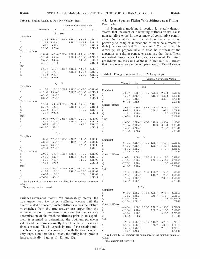
variance-covariance matrix. We successfully recover thetrue answer with the correct stiffness, whereas with theoverestimated or underestimated stiffness values the relativemismatches from the true answer are larger than theestimated errors. These results indicate that the accuratedetermination of the machine stiffness prior to an experi-ment is essential in determining the optimum parametervalues and their errors correctly if we treat the stiffness as afixed constant. This is especially true if the relative mis-match in the parameters associated with the shorter dc arevery large. Note that for all cases, the fitting looks great atleast graphically (Figures 11, 12, and 13).

4.5. Least Squares Fitting With Stiffness as a FittingParameter

[41] Numerical modeling in section 4.4 clearly demon-strated that incorrect or fluctuating stiffness values causenonnegligible errors in the estimate of constitutive param-eters. On the other hand, the stiffness variation is dueprimarily to complex interactions of machine elements attheir junctions and is difficult to control. To overcome thisdifficulty, we propose here to treat the stiffness of theapparatus as a fitting parameter assuming that the stiffnessis constant during each velocity step experiment. The fittingprocedures are the same as those in section 4.4.1, exceptthat there is one more unknown parameter, k. Table 4 shows

Table 1. Fitting Results to Positive Velocity Stepsa

Mismatch 2s

Variance-Covariance Matrix

a b dc fi

dc = 100Complianta �1.1E-3 6.6E-4b 1.1E-7 8.4E-8 �9.9E-8 �7.2E-10b �1.1E-3 5.8E-4b 8.4E-8 �8.4E-8 �3.1E-12dc 3.6E-4 9.5E-4 2.3E-7 1.1E-11fi 2.2E-6 9.7E-6 2.3E-11Correct stiffnessa �1.0E-4 6.2E-4 9.7E-8 7.5E-8 �8.8E-8 �6.3E-10b �2.1E-4 5.5E-4 7.5E-8 �7.5E-8 �1.2E-12dc 9.6E-5 9.0E-4 2.0E-7 8.8E-12fi �2.1E-6 1.1E-6 2.1E-11Stiffa 5.6E-4 6.5E-4 1.1E-7 8.2E-8 �9.6E-8 �6.9E-10b 4.4E-4 5.7E-4 8.2E-8 �8.2E-8 �3.3E-12dc �1.8E-5 9.4E-4 2.2E-7 8.1E-12fi �4.2E-6 9.5E-6 2.3E-11

dc = 10Complianta �1.3E-2 1.1E-3b 3.0E-7 2.2E-7 �2.6E-7 �2.2E-09b �1.2E-2 9.3E-4b 2.1E-7 �2.1E-7 �8.5E-11dc �6.3E-3 1.5E-3b 5.7E-7 4.5E-10fi 8.8E-5 1.7E-5b 6.9E-11Correct stiffnessa �2.3E-4 5.8E-4 8.5E-8 6.2E-8 �7.6E-8 �6.4E-10b 2.5E-4 5.0E-4 6.2E-8 �6.1E-8 �2.1E-11dc �3.2E-5 8.1E-4 1.7E-7 1.2E-10fi 1.3E-6 9.0E-6 2.0E-11Stiffa 8.9E-3 9.9E-4b 2.5E-7 1.8E-7 �2.2E-7 �1.9E-09b 7.6E-3 8.5E-4b 1.8E-7 �1.8E-7 �5.4E-11dc 7.6E-3 1.4E-3b 4.9E-7 3.2E-10fi �6.8E-5 1.5E-5b 6.0E-11

dc = 1Complianta �5.8E-2 2.2E-3b 1.2E-6 8.3E-7 �1.8E-6 �1.1E-08b �4.8E-2 1.6E-3b 6.4E-7 �1.1E-6 �4.7E-09dc �4.6E-2 3.4E-3b 2.9E-6 1.5E-08fi 4.7E-4 2.7E-5b 1.9E-10Correct stiffnessa �2.0E-9 6.4E-4 1.0E-7 6.3E-8 �1.1E-7 �1.1E-09b �3.6E-9 4.2E-4 4.4E-8 �7.0E-8 �5.4E-10dc �4.5E-9 7.8E-4 1.5E-7 1.1E-09fi �7.6E-6 8.9E-6 2.0E-11Stiffa 5.8E-2 1.3E-3b 4.2E-7 3.2E-7 �6.5E-7 �2.9E-09b 4.1E-2 1.1E-3b 2.8E-7 �4.3E-7 �1.1E-09dc 4.0E-3 2.2E-3b 1.2E-6 5.3E-09fi �7.6E-4 1.6E-5b 6.6E-11

aSee Figure 11. All numbers are normalized by the optimum parametervalues.

bTrue answer not recovered.

Table 2. Fitting Results to Negative Velocity Stepsa

Mismatch 2s


a b dc fi

dc = 100Complianta 3.8E-4 6.5E-4 1.1E-7 8.2E-8 �9.6E-8 6.7E-10b 7.3E-4 5.7E-4b 8.1E-8 �8.2E-8 1.1E-11dc �1.7E-3 9.3E-4b 2.2E-7 �1.4E-11fi �9.4E-6 9.3E-6b 2.2E-11Correct stiffnessa �3.6E-4 6.4E-4 1.0E-8 7.9E-8 �9.3E-8 6.4E-10b �6.0E-5 5.6E-4 7.9E-8 �8.0E-8 1.2E-11dc 1.1E-4 9.1E-4 2.1E-7 �1.3E-11fi �5.0E-6 9.1E-6 2.1E-11Stiffa �1.0E-3 6.5E-4b 1.0E-7 8.1E-8 �9.5E-8 6.6E-10b �7.1E-4 5.7E-4b 8.1E-8 �8.1E-8 1.1E-11dc 1.4E-3 9.2E-4b 2.1E-7 �1.0E-11fi �3.1E-6 9.2E-6 2.1E-11

dc = 10Complianta 6.1E-3 8.2E-4b 1.7E-7 1.3E-7 �1.6E-7 9.7E-10b 6.4E-3 7.1E-4b 1.3E-7 �1.4E-7 1.6E-10dc �1.5E-2 1.1E-3b 3.1E-7 �1.6E-10fi 3.1E-5 1.0E-5b 2.7E-11Correct stiffnessa �1.0E-4 7.0E-4 1.2E-7 9.6E-8 �1.1E-7 7.1E-10b �1.3E-4 6.1E-4 9.2E-8 �9.8E-8 1.0E-10dc �7.7E-5 9.5E-4 2.2E-7 �1.1E-10fi 6.1E-7 5.9E-6 2.0E-11Stiffa �5.7E-3 7.7E-4b 1.5E-7 1.2E-7 �1.3E-7 8.7E-10b �5.9E-3 6.7E-4b 1.1E-7 �1.2E-7 1.2E-10dc 1.2E-2 1.1E-3b 2.8E-7 �1.2E-10fi 2.6E-5 1.0E-5b 2.5E-11

dc = 1Complianta 9.1E-3 2.1E-3b 1.1E-6 8.9E-7 �9.7E-7 5.0E-09b 1.3E-2 1.8E-3b 7.8E-7 �8.3E-7 2.9E-09dc �5.8E-2 2.2E-3b 1.1E-6 �3.1E-09fi �2.3E-4 1.6E-5b 6.5E-11Correct stiffnessa �4.4E-4 1.0E-3 2.7E-7 2.2E-7 �2.5E-7 1.3E-09b �5.3E-4 8.9E-4 2.0E-7 �2.1E-7 7.4E-10dc 4.3E-4 1.1E-3 3.2E-7 �7.5E-10fi 3.0E-6 8.6E-6 1.9E-11Stiffa �1.9E-2 1.7E-3b 7.4E-7 6.1E-7 �6.7E-7 3.6E-09b �2.2E-2 1.5E-3b 5.4E-7 �5.8E-7 1.8E-09dc 5.6E-2 1.9E-3b 9.1E-7 �1.6E-09fi 1.8E-4 1.5E-5b 5.4E-11

aSee Figure 12. All numbers are normalized by the optimum parametervalues.

bTrue answer not recovered.


14 of 29

B04409

the resulting relative mismatches (deviation of each param-eter from its true value), normalized covariance matrix, andtwice the standard deviations obtained by the least squaresfitting to the same data as for Table 3. The curve fitting is asgraphically good as in the case with the correct stiffness inFigure 13 and is not shown here since there is no visibledifference between them at the scale of the plot. The relativemismatches for all parameters, including the stiffness, aresmaller than 2s, so that not only the optimum parametervalues are successfully determined, but also the length ofthe error bars. In the inversion of the real friction data ofHanaore fault gouge, we adopted the method described

here. We believe that our procedures have general applica-bility to other testing machines.

5. Constitutive Parameters of Hanaore FaultGouge

[42] Figure 14a shows the mechanical behavior of theblack clayey fault gouge in BAF046. Peak stress at theinitial yielding is not significant. The absolute value offriction coefficient is from about 0.43 to 0.62 with displace-ment hardening throughout the experiments. The overallmechanical behavior is similar to an experiment of 70%quartz and 30% smectite gouge by Saffer and Marone[2003] including the rate of strain hardening. Note thatthe scale of horizontal axis in our work is very different interms of shear strain from theirs. It should be emphasizedthat the rate of overall hardening per unit shear strain is inthe same order as in the work by Saffer and Marone [2003].We conducted another experiment, BAF045 at identicalconditions to BAF046 in terms of the way of waterinfiltration, the normal stress, and the range of load pointvelocities. Its overall behavior (the weak appearance ofinitial peak at the yielding, absolute value of friction, andthe rate of strain hardening) is almost identical to BAF 046and is therefore not shown here.[43] Figure 15a shows an example of mechanical behav-

ior on a velocity step at low strain rate (BAF046-11,indicated in Figure 14a). The shape of the peak after stepis symmetric and different from one observed in an approx-imately ideal velocity step (Figures 11a and 12a). Thissuggests that state evolution before shear stress reaches itsmaximum value is not negligible. In such cases, it isimportant to treat the stiffness of the apparatus as one ofthe fitting parameters in order to determine the constitutiveparameters, as shown in section 4. The optimum fittingcurves themselves are not plotted since it is very difficult torecognize the differences from the data. Instead, the resid-

Figure 13. Synthesized experimental data of positivevelocity steps by a factor of 10 with two state variablestogether with the best fit curves with fixed stiffness of theapparatus with dc1 = 10 and dc2 = 1. Two dashed linesrepresent the best fit curves with 10% higher and lowervalues of the stiffness of the apparatus, k. Note that thefitting looks excellent graphically although the relative errorfrom the true answer is large (Table 3).

Table 3. Fitting Results to Positive Velocity Steps With Two State Variables dc1 = 1 and dc2 = 10a

Mismatch 2s


a b1 dc1 b2 dc2 fi

Complianta 1.2E-1 4.6E-3b 5.4E-6 8.4E-6 �1.3E-5 1.5E-6 �1.2E-6 �2.6E-09b1 1.9E-1 7.5E-3b 1.4E-5 �1.9E-5 1.5E-6 �9.4E-7 �3.1E-09dc1 �5.5E-1 1.3E-2b 3.9E-5 �5.5E-6 4.9E-6 3.1E-09b2 2.3E-2 2.3E-3b 1.4E-6 �1.4E-6 9.8E-11dc2 �1.9E-2 2.9E-3b 2.1E-6 3.4E-11fi 4.6E-6 1.2E-5b 3.5E-11Correct stiffnessa �9.5E-4 2.6E-3 1.6E-6 2.4E-6 �4.9E-6 8.1E-7 �6.1E-7 �1.3E-09b1 �2.0E-3 4.3E-3 4.6E-6 �5.3E-6 1.5E-7 1.9E-7 �1.3E-09dc1 5.8E-3 8.9E-3 2.0E-5 �4.2E-6 3.6E-6 1.6E-09b2 �4.9E-4 2.4E-3 1.4E-6 �1.3E-6 �3.0E-11dc2 2.3E-4 2.6E-3 1.7E-6 8.1E-11fi �5.6E-6 9.1E-6 2.1E-11Stiffa �7.0E-2 2.7E-3b 1.8E-6 2.1E-6 �6.1E-6 1.4E-6 �9.7E-7 �1.8E-09b1 �1.1E-1 4.9E-3b 6.1E-6 �2.0E-6 �1.6E-6 1.9E-6 �1.3E-09dc1 2.7E-1 1.1E-2b 4.1E-6 �9.5E-6 7.4E-6 2.4E-09b2 �3.0E-2 4.0E-3b 4.1E-6 �3.5E-6 �1.9E-10dc2 2.0E-2 3.9E-3b 3.9E-6 2.1E-10fi �2.4E-5 1.1E-5b 3.4E-11

aSee Figure 13. All numbers are normalized by the optimum parameter values.bTrue answer not recovered.


15 of 29

B04409

uals from the best fit cases are plotted in Figure 15b for theslip law (upper) and the aging law (lower). The level ofrandom noise is on the order of 10�4 in the frictioncoefficient in our experimental condition, but the maximumamplitude of the residual is larger almost by an order ofmagnitude, which appear typically during the peak due tothe direct effect. All the fitting results are tabulated inTables 5 and 6 for the slip law and the aging law, respectively.Figure 14b shows the stiffness of the apparatus determinedfor each velocity step using the slip law. Error bars indicatetwice the standard deviation determined by the numericalfittings. Although each point is determined well, the stiffnessvalue scatters. In many cases, k ranges between 1300 to2200 m�1 with exceptionally large numbers which corre-spond to long error bars.[44] Figures 16 and 17 represent determined constitutive

parameters in the slip law and the aging law, respectively,plotted as a function of the geometric mean of the slip ratesbefore and after the velocity steps. Several parameters (b1,and dc1 for BAF45-1, -3, and BAF046-1 with the aging law,dc1 and dc2 for BAF046-3 and a, b1, and b2 for BAF046-15with the slip law) are not plotted in Figures 16 and 17 sincethey could not be determined precisely; 2s normalized bythe parameter value exceeded 1. Also, the respective valuesof BAF045-9 could not be determined because of thesampling interval was too long. Otherwise, the error barsare plotted only if they are longer than the symbol size.[45] The values of a � Sb were successfully determined

for all velocity steps (Figures 16a and 17a), and there is nosignificant difference between the two laws. The length ofthe error bar for a � Sb was estimated by using thevariance-covariance matrices listed in Tables 5 and 6.The a � Sb value changes its signature from negative topositive at a slip rate of around 0.1 mm s�1. Saffer andMarone [2003] also observed such a behavior but at adifferent slip rate (tens of microns per second) for themixture of quartz and smectites. Because we used muchthinner gouge layers than theirs, it is reasonable that weobserve this behavior at much lower slip rate if the sheardeformation is distributed over a width. This issue isdiscussed later.[46] Most of the a values determined are around 0.01 with

a few large values typically associated with long error bars(Figure 16b and 17b). This probably implies that the a valueis not very sensitive to the slip rate, which is consistent withthe interpretation of the direct effect by thermally activatedslip process at the solid-solid contacts [e.g., Nakatani, 2001;Rice et al., 2001; Noda, 2008].

[47] In many (22 out of 25) cases, two state variables arerequired to fit the experimental data, and all of them yieldb1 > b2 and dc2 > dc1. For the cases were the experimentalbehavior is able to fit by one state variable, these b and dc

Table 4. Fitting Results to Positive Velocity Steps With Two State Variables dc1 = 1 and dc2 = 10a

Mismatch 2s


k a b1 dc1 b2 dc2 fi

k �1.6E-3 2.3E-3 1.4E-6 �1.2E-6 �2.0E-6 4.9E-6 �3.6E-7 2.6E-7 �2.1E-10a 4.1E-4 3.3E-3 2.7E-6 �4.2E-6 �9.2E-6 1.1E-6 �8.4E-7 �1.1E-09b1 2.9E-4 5.5E-3 7.6E-6 �1.3E-5 7.0E-7 �2.2E-7 �9.5E-10dc1 1.3E-4 1.2E-2 3.7E-5 �5.5E-6 4.5E-6 8.9E-11b2 �8.1E-5 2.5E-3 1.5E-6 �1.4E-6 2.7E-11dc2 �7.2E-5 2.6E-3 1.7E-6 3.9E-11fi �5.3E-6 9.1E-6 2.0E-11

aSee Figure 13. All numbers are normalized by the optimum parameter values. The artificial experimental data is same as for Table 3, but stiffness of theapparatus is treated as one of the fitting parameters.

Figure 14. (a) A typical behavior of friction coefficientand integrated shear strain, g, and (b) determined machinestiffness, k, as a function of measured displacement with theslip law (black) and the aging law (gray). Note that themeasured displacement is used to calculate g so that the trueshear strain of the gouge layer is smaller than it especially atthe beginning of the loading where the simulated fault is notyet displaced.


16 of 29

B04409

are plotted as b1 and dc1 in Figures 16c, 17c, 16d, and 17dsince the value is close to them. Typically, a negative b2value is required to explain the experimental data atrelatively high slip rates, an example of which is shownin Figure 18 (BAF046-13). Similar to the a value, b1 is notremarkably dependent on the slip rate, but b2 seems todecrease and becomes negative around 1 mm s�1, althoughthe value scatters. In Figure 17d, dc1 might increase withincreases the slip rate, but the data points off the log-averaged value of dc1 have long error bars. In Figure 16d,the value of dc1 seems less scattered than in Figure 17dalthough there is one case which yields extremely short dc1.The dc2 seems to increase with slip rate (Figures 16d and17d) when the negative b2 appears. It should be emphasizedthat if a value is 0.01 and k is around 2000 m�1, a/k is about5 mm, and it is almost always important for us to treat k asone of the fitting parameters in our cases (see section 4).

6. Observation of Microstructure

[48] Figure 19 exhibits typical microstructures after theexperiments. The thickness of the gouge layer is about200 mm. The thin sections were made after specimens are

air dried, and during this process the black clayey faultgouge detaches from the host rocks.[49] Development of Y planes is rarely recognized, but

R1 planes are often observed which are typically detachedunder microscope because of the drying process but have apreferred orientation of platy minerals aligned along them.Between the R1 planes, preferred orientation of platyminerals is observed by forming bands with alternatingextinction positions (Figures 18c and 18d). These bandsare oriented at very high angle from R1 planes. From thecrosscutting relation, these bands are produced prior to theR1 planes.[50] Previous observations of simulated fault with gouge

suggest that the Y plane is developed after the initial peakstrength is achieved [Logan et al., 1992]. The poor devel-opment of Y planes is consistent with this statement sincepeak strength at the initial yielding is rarely observed. It isnotable that compared to the work by Saffer and Marone[2003], the a � Sb values changes its signature at a lowerslip rate, suggesting that the actual width of the shear zonedeveloped in the gouge layer is thinner in our study thantheirs. The observation supports the argument that strain isnot very well localized within the gouge layer by itself, butconfined by the gabbro blocks.[51] Unfortunately, the microstructures observed in the

natural outcrop (Figure 4) are not similar to one observedafter experiments. For example, the flow-like structure inFigure 4g is similar to one observed in a work by Mizoguchiand Shimamoto [2004] after high slip rate experimentswhich use much greater strain rate and total strain than inthis study. The structure in Figure 4i might suggest that thisblack clayey fault gouge was more indurated before the lastevent than the experiments in this work, and that deforma-tion mechanism is different. More experimental and micro-structural works may be needed to understand how thestructure seen on the outcrop is developed.

7. Discussion

[52] Experimental data from velocity step tests have beenanalyzed using a measured value of the machine stiffness asa fixed parameter, implicitly assumed to be free of error[e.g., Tullis and Weeks, 1986; Marone et al., 1990; Reinenand Weeks, 1993]. Our modeling results in Figures 11–13and Tables 1–3 clearly demonstrate that the relative mis-match of the constitutive parameters from the true answercan be larger in some cases than the half length of the errorbars (shown as 2s in Tables 1–3) if the assumed machinestiffness is incorrect. This error is serious when the criticaldisplacement, dc, is on the same order as the fault displace-ment from the abrupt change in the loading velocity to thepeak/bottom friction for the step increase/decrease in ve-locity (Tables 1–3). In such cases of small dc, the effect ofan incorrect value of k in shifting the optimum values of theconstitutive parameters becomes more important than theeffect of superposed random error on the same order as thereal experiment of a good quality. Traditional methods ofusing a fixed stiffness should not be used when dc is lessthan at least 100 a/k as shown in the numerical experimentsin this work. The stiffness and its fluctuation and/or the faultdisplacement to peak/bottom friction are not reported indetail in previous work and we cannot comment on the

Figure 15. (a) A plot of change in friction coefficient at avelocity step from 0.1554 to 1.54 mm s�1 (labeled inFigure 14a) after removing the trend. Rather symmetricalshape (unlike in Figure 1) of the peak implies that stateevolution is effective before the peak so that constitutiveparameters cannot be determined accurately because ofuncertainty in stiffness of the apparatus. (b) The residualsfor the best fit curves with (top) the slip law and (bottom)the aging law. The best fit curves themselves are notplotted since they are too close to see the difference.


17 of 29

B04409

Table 5. The Results With the Slip Law

Parameter Value Relative 2s

Normalized Variance-Covariance Matrix


BAF045-1, Load Point Velocity of 15.54 to 1.54 mm/sk (mm�1) 2.51E+0 7.7E-2 1.5E-3 �2.7E-4 �5.1E-6 5.8E-5 6.9E-4 �9.7E-5 3.6E-07a 7.56E-3 2.1E-2 1.1E-4 1.8E-6 �2.4E-5 �2.6E-4 3.8E-5 3.7E-07b1 3.74E-3 3.7E-2 3.4E-6 �2.0E-5 �4.0E-4 2.2E-5 9.7E-08dc1 (mm) 1.52E+1 1.0E-2 2.5E-5 1.1E-4 3.7E-5 1.6E-08b2 �3.82E-3 5.9E-2 8.6E-4 �1.7E-4 �7.6E-09dc2 (mm) 2.09E+2 2.0E-2 1.0E-4 8.8E-10fi 5.18E-1 2.1E-4 1.1E-08

BAF045-2, Load Point Velocity of 1.54 to 15.54 mm/sk (mm�1) 1.33E+0 2.4E-2 1.4E-4 �4.9E-5 �9.6E-5 2.1E-5 2.1E-4 �1.6E-4 �9.9E-10a 8.91E-3 1.6E-2 6.4E-5 1.3E-4 �2.1E-5 �2.1E-4 1.9E-4 �2.6E-09b1 3.92E-3 3.3E-2 2.8E-4 �3.1E-5 �3.7E-4 6.6E-5 �1.1E-09dc1 (mm) 1.58E+1 4.1E-2 4.2E-4 1.1E-4 6.1E-4 1.2E-10b2 �8.80E-4 6.2E-2 9.6E-4 �1.2E-3 1.1E-09dc2 (mm) 4.19E+2 1.6E-1 6.4E-3 �4.8E-10fi 5.09E-1 1.9E-5 8.6E-11

BAF045-3, Load Point Velocity of 15.54 to 1.54 mm/sk (mm�1) 2.75E+0 6.8E-2 1.2E-3 �2.0E-4 �3.0E-4 8.1E-5 4.5E-4 �1.0E-4 5.4E-08a 8.43E-3 1.8E-2 7.8E-5 1.1E-4 �3.2E-5 �1.7E-4 4.0E-5 4.0E-08b1 4.98E-3 2.7E-2 1.8E-4 �2.0E-5 �2.2E-4 1.6E-5 4.6E-09dc1 (mm) 1.66E+1 1.6E-2 6.3E-5 1.2E-4 �8.0E-5 1.1E-09b2 �2.49E-3 4.4E-2 4.9E-4 �1.7E-4 9.3E-10dc2 (mm) 2.38E+2 2.7E-2 1.8E-4 �6.8E-10fi 5.65E-1 7.2E-5 1.3E-09

BAF045-4, Load Point Velocity of 1.54 to 0.1554 mm/sk (mm�1) 2.53E+0 3.8E-2 3.7E-4 �7.7E-5 �5.2E-5 1.3E-4 2.2E-4 �8.0E-5 3.7E-07a 1.10E-2 1.6E-2 6.4E-5 4.3E-5 �6.3E-5 �1.2E-4 4.2E-5 3.7E-07b1 8.85E-3 1.4E-2 5.0E-5 �6.3E-6 �6.1E-5 �4.7E-6 5.7E-08dc1 (mm) 1.03E+1 2.6E-2 1.7E-4 2.0E-4 �1.3E-4 9.4E-09b2 �3.69E-3 3.5E-2 3.1E-4 �1.4E-4 �4.1E-08dc2 (mm) 7.35E+1 2.3E-2 1.3E-4 �1.2E-08fi 5.57E-1 2.4E-4 1.5E-08

BAF045-5, Load Point Velocity of 0.1554 to 0.0154 mm/sk (mm�1) 1.97E+0 4.0E-3 4.1E-6 �2.7E-6 9.9E-7 �2.8E-5 8.2E-6 1.8E-5 3.2E-09a 9.26E-3 3.9E-3 3.7E-6 �8.1E-7 3.3E-5 �9.4E-6 �2.1E-5 4.1E-09b1 8.88E-3 3.5E-3 3.1E-6 �2.8E-5 5.0E-6 2.2E-5 2.1E-09dc1 (mm) 5.65E+0 4.3E-2 4.5E-4 �1.1E-4 �3.2E-4 �2.7E-09b2 1.19E-3 1.1E-2 2.8E-5 7.1E-5 �3.6E-12dc2 (mm) 2.43E+1 3.1E-2 2.4E-4 1.9E-09fi 5.48E-1 1.9E-5 9.5E-11

BAF045-6, Load Point Velocity of 0.0154 to 0.1554 mm/sk (mm�1) 1.43E+0 5.1E-3 6.5E-6 �4.1E-6 �2.6E-6 �6.2E-6 2.0E-5 3.8E-6 �4.3E-10a 9.03E-3 7.3E-3 1.3E-5 9.2E-6 1.9E-5 �4.3E-5 �1.2E-5 �2.9E-10b1 6.07E-3 8.0E-3 1.6E-5 �4.4E-6 �1.6E-5 8.2E-6 �2.4E-10dc1 (mm) 5.67E+0 1.6E-2 6.0E-5 �8.6E-5 �4.8E-5 2.5E-10b2 3.30E-3 2.6E-2 1.7E-4 6.1E-5 �2.2E-10dc2 (mm) 3.96E+1 1.4E-2 4.7E-5 �5.1E-11fi 5.51E-1 5.8E-6 8.3E-12

BAF045-7, Load Point Velocity of 0.1554 to 1.54 mm/sk (mm�1) 1.87E+0 9.7E-3 2.3E-5 �1.8E-5 �2.4E-5 �1.7E-5 6.5E-5 1.1E-5 �6.0E-11a 1.26E-2 1.1E-2 3.0E-5 3.7E-5 3.6E-5 �9.9E-5 �2.3E-5 �3.5E-10b1 7.10E-3 1.5E-2 5.8E-5 1.8E-5 �1.1E-4 �5.5E-6 �3.0E-10dc1 (mm) 5.45E+0 2.0E-2 1.0E-4 �1.6E-4 �8.0E-5 5.6E-12b2 3.12E-3 3.8E-2 3.7E-4 1.1E-4 3.0E-10dc2 (mm) 4.33E+1 1.8E-2 7.8E-5 1.7E-11fi 5.53E-1 6.2E-6 9.6E-12



18 of 29

B04409

Table 5. (continued)




BAF045-9,a Load Point Velocity of 15.54 to 155.54 mm/sa-Sb 5.4E-3 2.2E-2

BAF045-10, Load Point Velocity of 155.54 to 15.54 mm/sk (mm�1) 2.35E+0 1.3E-1 4.3E-3 �7.0E-4 �1.1E-3 1.2E-3 2.6E-7a 1.19E-2 3.2E-2 2.5E-4 3.7E-4 �4.0E-4 3.1E-7b1 7.76E-3 4.8E-2 5.7E-4 �6.1E-4 8.5E-8dc1 (mm) 1.57E+1 5.7E-2 8.0E-4 �2.4E-8fi 6.21E-1 2.1E-4 1.1E-8

BAF046-1, Load Point Velocity of 15.54 to 1.54 mm/sk (mm�1) 3.07E+0 4.0E-2 4.0E-4 �1.9E-5 �3.6E-7 4.9E-5 6.7E-5 �6.0E-5 1.6E-07a 6.63E-3 7.5E-3 1.4E-5 4.2E-6 �1.3E-5 �1.9E-5 1.6E-5 1.1E-07b1 6.92E-3 7.4E-3 1.4E-5 1.9E-5 8.7E-6 �3.4E-5 7.2E-09dc1 (mm) 3.27E+1 1.6E-2 6.7E-5 5.7E-5 �9.3E-5 7.2E-09b2 �2.81E-3 1.6E-2 6.5E-5 �7.9E-5 5.3E-09dc2 (mm) 2.44E+2 2.7E-2 1.8E-4 �8.0E-09fi 4.71E-1 1.2E-4 3.5E-09

BAF046-2, Load Point Velocity of 1.54 to 0.1554 mm/sk (mm�1) 1.88E+0 6.3E-3 9.8E-6 �9.7E-6 �7.1E-6 �2.3E-5 2.4E-5 1.2E-5 1.0E-09a 1.18E-2 7.0E-3 1.2E-5 8.6E-6 3.1E-5 �3.1E-5 �1.7E-5 1.4E-09b1 8.39E-3 5.7E-3 8.1E-6 1.4E-5 �1.9E-5 �6.2E-6 7.4E-10dc1 (mm) 5.09E+0 2.0E-2 1.0E-4 �8.5E-5 �6.4E-5 �4.7E-10b2 2.34E-3 1.8E-2 7.9E-5 4.9E-5 �1.9E-10dc2 (mm) 2.38E+1 1.3E-2 4.2E-5 1.8E-10fi 4.81E-1 1.5E-5 5.5E-11

BAF046-3, Load Point Velocity of 0.1554 to 0.0154 mm/sk (mm�1) 2.04E+0 9.1E-3 2.0E-5 �9.8E-6 �4.8E-7 6.5E-3 3.0E-5 1.2E-2 3.3E-08a 7.48E-3 7.4E-3 1.4E-5 2.9E-6 �6.5E-3 �2.9E-5 �1.2E-2 3.5E-08b1 7.41E-3 4.5E-3 5.2E-6 2.7E-3 5.3E-7 4.3E-3 1.5E-08dc1 (mm) 5.43E+0 5.5E+0 7.5E+0 2.0E-2 1.3E+1 2.0E-06b2 7.95E-5 1.8E-2 7.7E-5 3.5E-3 2.0E-09dc2 (mm) 1.15E+2 9.2E+0 2.1E+1 3.6E-06fi 4.88E-1 5.8E-5 8.3E-10

BAF046-4, Load Point Velocity of 0.0154 to 0.1554 mm/sk (mm�1) 1.40E+0 2.7E-3 1.8E-6 �9.9E-7 1.2E-6 �5.6E-6 6.8E-6 3.2E-6 �2.8E-10a 7.11E-3 3.5E-3 3.1E-6 �1.9E-6 1.4E-5 �1.3E-5 �8.0E-6 �2.2E-10b1 4.66E-3 7.8E-3 1.5E-5 �3.7E-5 2.2E-5 2.8E-5 �2.4E-10dc1 (mm) 6.44E+0 2.2E-2 1.2E-4 �8.8E-5 �8.2E-5 3.3E-10b2 2.21E-3 1.7E-2 7.6E-5 5.6E-5 �1.6E-10dc2 (mm) 2.91E+1 1.6E-2 6.5E-5 �1.1E-10fi 4.10E-1 4.8E-6 5.7E-12

BAF046-5, Load Point Velocity of 0.1554 to 1.54 mm/sk (mm�1) 1.86E+0 4.9E-3 6.0E-6 �3.9E-6 �5.7E-6 �3.5E-6 1.6E-5 2.5E-6 �3.3E-11a 1.06E-2 5.0E-3 6.2E-6 8.6E-6 6.5E-6 �2.2E-5 �4.7E-6 �1.4E-10b1 5.52E-3 7.8E-3 1.5E-5 2.5E-6 �2.5E-5 �3.7E-7 �1.1E-10dc1 (mm) 6.29E+0 8.8E-3 1.9E-5 �3.2E-5 �1.6E-5 �2.6E-12b2 2.78E-3 1.9E-2 8.9E-5 2.5E-5 1.1E-10dc2 (mm) 5.53E+1 8.5E-3 1.8E-5 8.3E-12fi 4.95E-1 4.2E-6 4.3E-12

BAF046-6,Load Point Velocity of 1.54 to 15.54 mm/sk (mm�1) 1.41E+0 1.6E-2 6.8E-5 �1.8E-5 �3.8E-5 �4.0E-5 7.8E-5 �8.0E-5 �5.3E-10a 8.96E-3 9.0E-3 2.0E-5 4.2E-5 3.8E-5 �6.4E-5 7.6E-5 �1.3E-09b1 3.96E-3 1.9E-2 9.1E-5 1.9E-5 �1.2E-4 4.3E-5 �5.2E-10dc1 (mm) 1.58E+1 7.3E-2 1.3E-3 �2.5E-4 2.3E-3 �1.2E-10b2 �2.20E-3 3.4E-2 2.9E-4 �4.9E-4 4.8E-10dc2 (mm) 1.01E+3 1.2E-1 3.9E-3 �2.5E-10fi 5.10E-1 1.3E-5 4.3E-11

BAF046-7, Load Point Velocity of 15.54 to 1.54 mm/sk (mm�1) 1.76E+0 1.6E-2 6.2E-5 �6.8E-5 �1.2E-4 2.0E-7 1.1E-4 �7.7E-6 2.1E-08a 1.18E-2 1.9E-2 9.4E-5 1.7E-4 �2.0E-7 �1.5E-4 1.2E-5 1.1E-08b1 6.49E-3 3.5E-2 3.0E-4 �4.3E-7 �2.7E-4 2.1E-5 2.5E-09dc1 (mm) 5.08E+0 2.5E-3 1.5E-6 1.5E-7 3.3E-6 4.0E-11b2 �2.89E-3 3.1E-2 2.4E-4 �2.3E-5 2.4E-09dc2 (mm) 3.99E+2 8.2E-3 1.7E-5 �6.2E-10


19 of 29

B04409





fi 5.39E-1 4.5E-5 5.1E-10

BAF046-8, Load Point Velocity of 1.54 to 0.1554 mm/sk (mm�1) 2.06E+0 1.7E-2 6.8E-5 �2.3E-5 �2.9E-5 4.4E-5 7.4E-8a 1.31E-2 1.2E-2 3.4E-5 3.9E-5 �4.3E-5 1.2E-7b1 1.07E-2 1.4E-2 4.6E-5 �5.1E-5 �5.6E-8dc1 (mm) 5.96E+0 1.7E-2 6.8E-5 4.1E-8fi 5.34E-1 1.3E-4 4.2E-9

BAF046-9, Load Point Velocity of 0.1554 to 0.0154 mm/sk (mm�1) 2.04E+0 2.9E-2 2.2E-4 �1.3E-4 5.5E-6 �2.0E-3 3.7E-4 1.5E-3 1.6E-07a 8.71E-3 2.9E-2 2.0E-4 2.9E-5 2.4E-3 �4.4E-4 �1.9E-3 2.2E-07b1 8.72E-3 1.9E-2 9.2E-5 �8.9E-4 4.5E-5 1.0E-3 1.1E-07dc1 (mm) 4.54E+0 4.3E-1 4.6E-2 �6.8E-3 �4.0E-2 �1.2E-07b2 5.86E-4 6.8E-2 1.1E-3 5.6E-3 �2.6E-08dc2 (mm) 2.43E+1 4.0E-1 4.0E-2 1.2E-07fi 5.37E-1 1.3E-4 4.5E-09

BAF046-10, Load Point Velocity of 0.0154 to 0.1554 mm/sk (mm�1) 1.51E+0 8.0E-3 1.6E-5 9.0E-7 4.1E-6 �9.1E-6 1.7E-5 7.1E-6 �2.6E-09a 7.53E-3 6.6E-3 1.1E-5 8.0E-6 1.3E-5 �1.9E-5 �1.1E-5 �3.1E-09b1 6.45E-3 7.2E-3 1.3E-5 �1.0E-5 �1.3E-6 1.3E-5 �1.5E-09dc1 (mm) 9.07E+0 1.7E-2 7.2E-5 �6.1E-5 �6.9E-5 7.1E-10b2 2.18E-3 1.8E-2 7.8E-5 5.5E-5 1.3E-09dc2 (mm) 9.17E+1 2.0E-2 9.7E-5 �2.0E-10fi 5.40E-1 1.7E-5 6.8E-11

BAF046-11, Load Point Velocity of 0.1554 to 1.54 mm/sk (mm�1) 2.03E+0 5.0E-3 6.2E-6 �3.3E-6 �3.5E-6 �5.0E-6 1.5E-5 3.6E-6 �5.1E-11a 1.17E-2 4.9E-3 6.0E-6 6.5E-6 8.9E-6 �1.9E-5 �6.5E-6 �2.2E-10b1 7.09E-3 6.5E-3 1.0E-5 7.6E-7 �1.5E-5 1.5E-6 �1.4E-10dc1 (mm) 6.67E+0 1.2E-2 3.6E-5 �4.2E-5 �3.0E-5 �8.7E-12b2 2.74E-3 1.8E-2 7.7E-5 3.2E-5 1.7E-10dc2 (mm) 5.76E+1 1.2E-2 3.4E-5 1.7E-11fi 5.47E-1 5.1E-6 6.6E-12

BAF046-12, Load Point Velocity of 1.54 to 15.54 mm/sk (mm�1) 1.58E+0 1.4E-2 4.7E-5 �1.3E-5 �2.3E-5 �5.3E-6 5.2E-5 �1.8E-5 �5.1E-10a 1.02E-2 8.8E-3 1.9E-5 3.5E-5 6.4E-6 �5.0E-5 2.1E-5 �1.4E-09b1 5.26E-3 1.6E-2 6.7E-5 3.4E-6 �8.7E-5 1.4E-5 �6.0E-10dc1 (mm) 1.39E+1 2.0E-2 1.0E-4 �3.5E-5 2.1E-4 �2.4E-11b2 �2.84E-3 2.7E-2 1.9E-4 �1.1E-4 5.9E-10dc2 (mm) 1.02E+3 4.5E-2 5.0E-4 �9.6E-11fi 5.60E-1 1.4E-5 4.7E-11

BAF046-13, Load Point Velocity of 15.54 to 1.54 mm/sk (mm�1) 2.13E+0 2.7E-2 1.9E-4 �9.0E-5 �1.6E-4 4.2E-6 1.6E-4 �6.2E-6 8.1E-08a 1.10E-2 1.7E-2 7.1E-5 1.2E-4 �3.5E-6 �1.2E-4 5.2E-6 7.1E-08b1 6.10E-3 3.0E-2 2.2E-4 �5.5E-6 �2.2E-4 7.7E-6 2.6E-08dc1 (mm) 8.88E+0 2.3E-3 1.3E-6 8.5E-6 �1.5E-6 8.8E-10b2 �4.22E-3 3.1E-2 2.4E-4 �1.3E-5 �5.6E-09dc2 (mm) 4.06E+2 4.7E-3 5.5E-6 �5.9E-11fi 5.94E-1 9.9E-5 2.5E-09


BAF046-15, Load Point Velocity of 0.1554 to 0.0154 mm/sk (mm�1) 1.63E+0 2.3E-2 1.3E-4 �1.2E-2 �1.2E-2 �5.7E-5 1.2E-2 7.2E-5 2.2E-09a 1.08E-1 2.1E+0 1.1E+0 1.1E+0 5.2E-3 �1.1E+0 �6.5E-3 �7.8E-08b1 1.04E-1 2.1E+0 1.2E+0 5.5E-3 �1.2E+0 �6.8E-3 �8.1E-08dc1 (mm) 1.15E-1 1.1E-2 2.9E-5 �5.5E-3 �3.5E-5 �4.0E-10


20 of 29

B04409

validity of previous measurements of the constitutiveparameters.[53] The alternative and simple method we propose in this

paper is to treat the machine stiffness as an unknownparameter in exactly the same manner as the frictionalconstitutive parameters are treated. The results in Table 4show that all the constitutive parameters are recoveredwithin the estimated errors. We emphasize that there is noneed to determine the stiffness of the apparatus preciselyprior to experiments in this revised method. The onlyassumption we made is that the apparatus is linearly elasticin each velocity step portion of the experiment, but not inthe entire experiments like in the work by Blanpied et al.[1998]. We consider that this assumption is reasonable inview of the systematic loading behavior of our machine(Figure 9) and small amount of change in the frictioncoefficient relative to its absolute value. Note that time-dependent inelastic deformation of the apparatus probablybecomes important in experiments with extremely lowloading velocities. In such cases, the assumption we takeis no longer valid and the precise determination of theconstitutive parameters requires us to solve the coupling ofthe frictional surface and the elastic-plastic apparatus or thedetermined fault constitutive parameters are affected by theplastic deformation of the apparatus.[54] Reinen and Weeks [1993] discussed the effect of the

stiffness value as a fixed parameter since they can control itwhen using a high-speed servo-control system. They do nottreat the machine stiffness, k as a fitting parameter, and theerror in it is not reported in their variance-covariance matrix.Blanpied et al. [1998] determined k for each velocity stepusing the rate of change in the friction coefficient just afterthe velocity step and reported that it varied for one velocitystep to another. We think this method is reasonable althoughthey cannot determine the error bar in it. It is true that themachine stiffness affects the initial slope in friction coeffi-cient toward the peak friction due to the direct effect asshown in equation (9), but it also affects the overallfrictional behavior especially when one of the dc is verysmall. So, we think that it is more reasonable to determine kusing entire data set, not only just after the step.[55] Our biaxial apparatus was designed for high-temper-

ature friction experiments and its stiffness property is notideal; the machine is compliant and the stiffness variesconsiderably. This is because the specimen assembly in thefurnace consists of several elements such as ceramic pis-tons, temperature-resistant stainless-steel spacers, metalpistons and rock specimens [see Kawamoto andShimamoto, 1997, 1998]. We expect that most other similarmachines are superior with regards to the stiffness fluctua-tion. After investigating the mechanical property of theapparatus, we conclude that treating the machine stiffness

as an unknown parameter in the analysis of specimen-apparatus interaction for the velocity step test is the bestway to experimentally determine the fault constitutiveparameters at the present time. Of course, specimen-apparatus interaction does not have to be analyzed for theestimate of constitutive parameters if an ideal step change inslip rate along fault is attained in experiments by monitoringthe fault displacement and controlling it via servo-control.[56] We reemphasize that a big advantage of biaxial

machines [e.g., Hoskins et al., 1968; Dieterich, 1979,1981; Marone, 1998; Saffer and Marone, 2003] (our ma-chine) is their high sensitivity of friction measurementsbecause the loading column and the specimen assemblyare free from O-rings and jackets. Fault constitutive prop-erties are so subtle that we are not sure how much errors inthe estimate of constitutive parameters are induced, forinstance, by jacket strength and friction between the endof a precut specimen and piston in triaxial experiments or byO-ring or any other friction in rotary shear experiments.Despite the success of fault constitutive laws, we arecurrently faced with describing the complex constitutivebehavior of clayey fault gouges whose constitutive param-eters change substantially with ambient conditions and sliprate [e.g., Logan and Rauenzahn, 1987; Morrow et al.,2000; Bos et al., 2000; Niemeijer and Spiers, 2006]. Thiscould be due to partial operation of plastic deformation suchas basal plane slip in sheet silicate minerals. Under deeperconditions and at very slow slip rates under fluid-richenvironments, plastic deformation in granular mineralsand solution/precipitation creep may enter into the processes[e.g., Shimamoto, 1986; Bos and Spiers, 2002]. Thus,accurate measurements of constitutive parameters still re-main to be experimental challenges.[57] Figures 16 and 17 show that the data points scatter

much more widely than the error bars determined by leastsquares fitting for respective velocity steps so that theoverall error is determined by the experimental reproduc-ibility. From Tables 1–3, the relative mismatch is at most onthe order of 10%, and not by orders of magnitude. Thus, thenew method we adopted in this work might not make acritical difference in previously reported data, although thetreatment of the machine stiffness as one of the fittingparameter is essential to estimate mathematically correctoptimum parameter values and errors. Comparing the twoconstitutive laws (the slip law and the aging law), the sliplaw seems to do a better job since the data points seems soscatter widely in Figure 17 than in Figure 16.[58] Figure 20 is a magnified plot of the change in friction

coefficient (BAF046-5, -6, and -7, indicated in Figure 14a).Apparently, the slope of strain hardening is steeper at highslip rate (15.54 mm s�1) than at the lower slip rates, whichcan be recognized in Figure 14a as well. It is notable that




k a b1 dc1 b2 dc2 fib2 6.56E-3 2.2E+0 1.2E+0 6.9E-3 8.5E-08dc2 (mm) 8.00E+0 1.3E-2 4.3E-5 7.1E-10fi 5.89E-1 1.2E-5 3.9E-11

aOnly a � Sb was determined. The state evolution equation does not matter.


21 of 29

B04409

Table 6. The Results With the Aging Law




BAF045-1, Load Point Velocity of 15.54 to 1.54 mm/sk (mm�1) 2.44E+0 5.2E-2 6.8E-4 �3.9E-5 5.0E-3 5.0E-3 8.7E-4 �7.6E-4 2.8E-07a 7.50E-3 1.1E-2 3.0E-5 �2.1E-3 �2.1E-3 �3.7E-4 3.2E-4 2.6E-07b1 3.15E-2 1.5E+0 5.6E-1 5.6E-1 9.2E-2 �8.9E-2 �1.0E-06dc1 (mm) 9.51E+1 1.5E+0 5.6E-1 9.2E-2 �8.9E-2 �1.0E-06b2 �3.15E-2 2.5E-1 1.5E-2 1.5E-2 �1.9E-07dc2 (mm) 1.31E+2 2.4E-1 1.4E-2 1.6E-07fi 5.19E-1 1.8E-4 8.1E-09


BAF045-3, Load Point Velocity of 15.54 to 1.54 mm/sk (mm�1) 2.78E+0 5.2E-2 6.7E-4 �4.0E-5 3.8E-3 4.2E-3 7.3E-4 �6.5E-4 4.2E-08a 8.15E-3 9.5E-3 2.2E-5 �1.5E-3 �1.7E-3 �2.9E-4 2.6E-4 3.1E-08b1 2.82E-2 1.1E+0 3.1E-1 3.4E-1 5.6E-2 �5.5E-2 �5.0E-08dc1 (mm) 9.53E+1 1.2E+0 3.7E-1 6.1E-2 �6.0E-2 �5.5E-08b2 �2.59E-2 2.0E-1 1.0E-2 �9.8E-3 �1.0E-08dc2 (mm) 1.34E+2 2.0E-1 9.7E-3 8.2E-09fi 5.65E-1 6.3E-5 9.9E-10

BAF045-4, Load Point Velocity of 1.54 to 0.1554 mm/sk (mm�1) 2.43E+0 2.9E-2 2.2E-4 �7.1E-6 5.8E-4 7.5E-4 2.2E-4 �1.8E-4 4.2E-07a 1.16E-2 1.1E-2 3.3E-5 �3.8E-4 �5.1E-4 �1.5E-4 1.2E-4 4.0E-07b1 2.62E-2 2.5E-1 1.6E-2 2.1E-2 5.6E-3 �5.5E-3 �3.2E-07dc1 (mm) 3.07E+1 3.3E-1 2.7E-2 7.3E-3 �7.0E-3 �4.5E-07b2 �2.05E-2 8.9E-2 2.0E-3 �1.9E-3 �1.8E-07dc2 (mm) 5.48E+1 8.6E-2 1.8E-3 8.8E-08fi 5.57E-1 2.5E-4 1.6E-08

BAF045-5, Load Point Velocity of 0.1554 to 0.0154 mm/sk (mm�1) 1.74E+0 3.3E-3 2.7E-6 �3.2E-6 �1.5E-6 �5.4E-6 1.3E-5 3.2E-6 3.2E-09a 1.10E-2 5.5E-3 7.5E-6 2.9E-6 4.3E-5 �2.7E-5 �8.5E-6 3.1E-09b1 7.28E-3 6.1E-3 9.2E-6 �7.8E-6 �1.5E-6 8.4E-6 3.5E-09dc1 (mm) 4.18E+0 1.3E-2 4.4E-5 �6.3E-5 �3.3E-5 �2.2E-09b2 4.50E-3 2.1E-2 1.1E-4 4.3E-5 2.5E-09dc2 (mm) 2.35E+1 1.1E-2 2.8E-5 5.5E-10fi 5.48E-1 1.8E-5 8.1E-11

BAF045-6, Load Point Velocity of 0.0154 to 0.1554 mm/sk (mm�1) 1.50E+0 5.1E-3 6.5E-6 �1.5E-6 �3.4E-7 �4.7E-6 8.8E-6 3.0E-6 �3.8E-10a 8.22E-3 4.7E-3 5.6E-6 4.4E-6 8.3E-6 �1.1E-5 �5.2E-6 �3.4E-10b1 6.44E-3 5.6E-3 7.9E-6 �6.8E-6 �3.2E-6 6.2E-6 �1.7E-10dc1 (mm) 4.99E+0 1.5E-2 5.3E-5 �3.2E-5 �3.8E-5 1.6E-10b2 2.12E-3 1.2E-2 3.4E-5 2.1E-5 1.4E-11dc2 (mm) 2.80E+1 1.3E-2 5.0E-5 �4.0E-11fi 5.51E-1 5.8E-6 8.3E-12

BAF045-7, Load Point Velocity of 0.1554 to 1.54 mm/sk (mm�1) 1.98E+0 9.6E-3 2.3E-5 �9.9E-6 �1.2E-5 �1.3E-5 3.1E-5 7.7E-6 �8.3E-11a 1.15E-2 7.1E-3 1.3E-5 1.6E-5 1.6E-5 �3.1E-5 �1.0E-5 �3.4E-10b1 6.92E-3 1.0E-2 2.6E-5 �3.7E-7 �3.1E-5 3.1E-6 �2.0E-10dc1 (mm) 4.88E+0 1.9E-2 8.7E-5 �6.5E-5 �6.2E-5 �5.4E-12b2 2.17E-3 2.0E-2 9.6E-5 4.2E-5 1.5E-10dc2 (mm) 3.05E+1 1.6E-2 6.4E-5 1.3E-11fi 5.53E-1 6.5E-6 1.1E-11



22 of 29

B04409





BAF045-9,a Load Point Velocity of 15.54 to 155.54 mm/sa-Sb 5.40E-03 2.2E-2


BAF046-1, Load Point Velocity of 15.54 to 1.54 mm/sk (mm�1) 2.01E+0 1.5E-2 5.6E-5 3.8E-7 1.6E-3 1.8E-3 1.5E-4 �1.5E-4 4.6E-08a 7.67E-3 4.0E-3 4.0E-6 �9.1E-4 �9.9E-4 �8.4E-5 8.6E-5 3.5E-08b1 6.27E-2 1.9E+0 8.8E-1 9.6E-1 7.9E-2 �8.5E-2 �3.3E-07dc1 (mm) 1.12E+2 2.1E+0 1.1E+0 8.7E-2 �9.3E-2 �3.7E-07b2 �5.75E-2 1.7E-1 7.1E-3 �7.7E-3 �3.3E-08dc2 (mm) 1.34E+2 1.8E-1 8.2E-3 3.0E-08fi 4.71E-1 6.9E-5 1.2E-09

BAF046-2, Load Point Velocity of 1.54 to 0.1554 mm/sk (mm�1) 1.71E+0 5.5E-3 7.6E-6 �1.5E-5 �2.3E-5 �5.1E-6 3.9E-5 3.3E-6 1.1E-09a 1.46E-2 1.3E-2 4.0E-5 5.7E-5 1.7E-5 �1.0E-4 �1.2E-5 1.4E-09b1 8.72E-3 1.8E-2 8.4E-5 2.0E-5 �1.4E-4 �1.2E-5 1.3E-09dc1 (mm) 3.33E+0 8.0E-3 1.6E-5 �5.2E-5 �1.3E-5 �4.1E-10b2 4.82E-3 3.3E-2 2.7E-4 3.7E-5 3.0E-11dc2 (mm) 2.86E+1 7.0E-3 1.2E-5 2.1E-11fi 4.81E-1 1.5E-5 5.3E-11

BAF046-3, Load Point Velocity of 0.1554 to 0.0154 mm/sk (mm�1) 1.49E+0 1.4E-2 4.8E-5 �1.6E-3 �1.8E-3 1.2E-5 1.8E-3 �6.0E-6 3.2E-08a 4.14E-2 4.8E-1 5.8E-2 6.6E-2 �1.5E-4 �6.7E-2 �9.9E-6 �4.1E-07b1 3.63E-2 5.5E-1 7.5E-2 �1.8E-4 �7.6E-2 �7.7E-6 �4.8E-07dc1 (mm) 2.34E-1 8.5E-3 1.8E-5 1.5E-4 �1.8E-5 8.4E-09b2 5.05E-3 5.6E-1 7.8E-2 3.8E-5 5.1E-07dc2 (mm) 1.17E+1 9.3E-3 2.2E-5 �1.1E-08fi 4.88E-1 4.4E-5 4.8E-10

BAF046-4, Load Point Velocity of 0.0154 to 0.1554 mm/sk (mm�1) 1.45E+0 2.9E-3 2.1E-6 �5.0E-7 3.4E-7 �3.8E-6 3.1E-6 2.2E-6 �2.9E-10a 6.67E-3 2.6E-3 1.7E-6 6.3E-7 5.9E-6 �3.8E-6 �3.4E-6 �2.7E-10b1 5.12E-3 4.0E-3 4.0E-6 �1.2E-5 2.2E-6 9.2E-6 �1.4E-10dc1 (mm) 4.97E+0 1.7E-2 7.5E-5 �2.7E-5 �5.0E-5 2.2E-10b2 1.31E-3 7.6E-3 1.4E-5 1.7E-5 �6.9E-12dc2 (mm) 2.07E+1 1.3E-2 4.5E-5 �7.9E-11fi 4.90E-1 5.1E-6 6.5E-12


BAF046-6, Load Point Velocity of 1.54 to 15.54 mm/sk (mm�1) 1.45E+0 1.8E-2 8.2E-5 �2.2E-5 �5.0E-5 �8.0E-6 7.5E-5 �2.6E-5 �6.0E-10a 8.70E-3 9.0E-3 2.0E-5 4.7E-5 7.3E-6 �5.4E-5 2.2E-5 �1.4E-09b1 3.65E-3 2.1E-2 1.1E-4 �8.7E-7 �1.2E-4 3.3E-6 �5.4E-10dc1 (mm) 9.80E+0 3.8E-2 3.6E-4 �4.6E-5 6.0E-4 �1.1E-11b2 �1.51E-3 2.8E-2 2.0E-4 �1.4E-4 3.1E-10dc2 (mm) 3.16E+2 6.7E-2 1.1E-3 �4.9E-11fi 5.10E-1 1.4E-5 4.8E-11

BAF046-7, Load Point Velocity of 15.54 to 1.54 mm/sk (mm�1) 1.79E+0 1.1E-2 3.0E-5 �2.5E-5 �4.5E-5 �1.9E-6 5.4E-5 �1.2E-5 1.5E-08a 1.16E-2 1.1E-2 3.2E-5 5.5E-5 3.1E-6 �6.9E-5 1.8E-5 9.6E-09b1 6.37E-3 2.0E-2 9.8E-5 4.8E-6 �1.2E-4 2.8E-5 3.4E-09dc1 (mm) 7.74E+0 4.1E-3 4.2E-6 �9.1E-6 1.4E-5 �1.7E-10b2 �3.96E-3 2.5E-2 1.6E-4 �5.0E-5 5.0E-10dc2 (mm) 1.50E+3 1.5E-2 5.4E-5 �1.0E-09


23 of 29

B04409





fi 5.39E-1 3.9E-5 3.9E-10


BAF046-9, Load Point Velocity of 0.1554 to 0.0154 mm/sk (mm�1) 1.65E+0 3.5E-2 3.1E-4 �1.3E-3 �1.8E-3 �1.5E-4 2.5E-3 8.7E-5 1.9E-07a 1.51E-2 1.8E-1 7.7E-3 1.0E-2 1.3E-3 �1.4E-2 �9.1E-4 4.3E-08b1 1.08E-2 2.3E-1 1.3E-2 1.6E-3 �1.9E-2 �1.0E-3 �1.2E-08dc1 (mm) 1.29E+0 5.0E-2 6.4E-4 �2.9E-3 �5.7E-4 �4.0E-08b2 4.83E-3 3.3E-1 2.8E-2 2.1E-3 3.7E-07dc2 (mm) 1.49E+1 5.0E-2 6.1E-4 �2.9E-08fi 5.37E-1 1.3E-4 4.2E-09

BAF046-10, Load Point Velocity of 0.0154 to 0.1554 mm/sk (mm�1) 1.59E+0 1.2E-2 3.5E-5 1.2E-6 4.0E-6 �1.0E-5 1.9E-5 6.8E-6 �3.3E-09a 7.19E-3 7.0E-3 1.2E-5 1.1E-5 7.4E-6 �1.4E-5 �5.7E-6 �4.0E-09b1 6.52E-3 7.6E-3 1.5E-5 �7.9E-6 �6.8E-6 7.7E-6 �1.3E-09dc1 (mm) 5.91E+0 1.5E-2 5.9E-5 �3.2E-5 �4.7E-5 4.7E-10b2 1.76E-3 1.3E-2 4.2E-5 2.5E-5 1.3E-09dc2 (mm) 5.52E+1 1.7E-2 7.3E-5 �3.1E-11fi 5.40E-1 1.9E-5 8.8E-11


BAF046-12, Load Point Velocity of 1.54 to 15.54 mm/sk (mm�1) 1.60E+0 1.4E-2 4.9E-5 �1.5E-5 �2.9E-5 8.4E-8 4.7E-5 �4.9E-6 �4.7E-10a 9.98E-3 8.6E-3 1.9E-5 3.7E-5 1.5E-7 �4.1E-5 5.5E-6 �1.3E-99b1 4.95E-3 1.7E-2 7.3E-5 �4.1E-7 �7.9E-5 1.9E-6 �5.6E-10dc1 (mm) 8.39E+0 1.0E-2 2.7E-5 �1.1E-6 4.5E-5 1.2E-12b2 �2.18E-3 2.3E-2 1.3E-4 �2.8E-5 �3.7E-10dc2 (mm) 3.78E+2 2.2E-2 1.3E-4 1.5E-11fi 5.60E-1 1.3E-5 4.4E-11

BAF046-13, Load Point Velocity of 15.54 to 1.54 mm/sk (mm�1) 2.73E+0 3.8E-2 3.7E-4 �3.4E-5 �3.4E-5 2.7E-5 1.5E-4 �3.5E-5 2.5E-07a 9.03E-3 1.0E-2 2.7E-5 1.9E-5 �1.3E-5 �7.2E-5 1.7E-5 1.7E-07b1 5.84E-3 1.3E-2 4.4E-5 1.2E-5 �1.2E-5 �2.4E-5 1.5E-08dc1 (mm) 4.34E+1 1.0E-2 2.7E-5 8.6E-5 �4.2E-5 �2.5E-10b2 �6.04E-3 3.8E-2 3.6E-4 �1.2E-4 �1.3E-08dc2 (mm) 5.95E+2 1.8E-2 7.7E-5 1.4E-09fi 5.94E-1 1.5E-4 5.6E-09


BAF046-15, Load Point Velocity of 0.1554 to 0.0154 mm/sk (mm�1) 1.58E+0 3.5E-3 3.0E-6 �8.3E-5 �9.3E-5 2.1E-7 9.8E-5 8.4E-7 7.7E-10a 4.43E-2 1.0E-1 2.7E-3 3.0E-3 9.9E-6 �3.2E-3 �4.8E-5 �3.4E-09b1 3.92E-2 1.2E-1 3.4E-3 1.1E-5 �3.6E-3 �5.4E-5 �3.9E-09dc1 (mm) 2.78E-1 2.1E-3 1.2E-6 �1.3E-5 �2.0E-6 2.1E-11b2 6.87E-3 1.2E-1 3.8E-3 6.0E-5 5.6E-09


24 of 29

B04409

typically in the following negative velocity steps evolutionof friction coefficient shows a behavior with a negative b2value; a peak followed by rapid decay and another slowdecay in the opposite direction. This implies that theapparently steeper displacement strengthening is due toevolution of second state variable with negative b2 andlong dc2, and indeed, they are required in the numericalfittings. The upward convexity observed at the high slip

rate (15.54 mm s�1) might include some contribution fromthe overall hardening behavior which is convex upward,but it must have only a minor effect since the rate ofhardening is apparently too high at 15.54 mm s�1, and itcannot explain the second decay in the following velocitystep.[59] Dilatation of the gouge layer and following fluid

transportation might affect measured friction coefficient




k a b1 dc1 b2 dc2 fidc2 (mm) 1.53E+1 4.5E-3 5.1E-6 �1.4E-10fi 5.89E-1 8.5E-6 1.8E-11

aOnly a � Sb was determined. The state evolution equation does not matter.

Figure 16. The constitutive parameters determined by numerical least squares fitting with the slip law.The horizontal axes are geometric mean of the slip rates before and after the velocity steps. The error bars(±2s) are plotted only when they are longer than the symbol size. If the error is larger than the absolutevalue of the corresponding optimum parameter value, such a point is not plotted. All results are listed inTable 5. (a) The a � Sb values are determined for all velocity steps. The a � Sb value is negative at alow slip rate and becomes positive at higher slip rates. (b) The a value seems independent of the slip rate.(c) The b values. The b1 and b2 are defined so that dc1 < dc2. If the experimental data are fit well by onlyone state variable, b is treated as b1. Typically, at a higher slip rate, a negative b2 is required to fit themechanical behavior of the fault. (d) The dc values. The dc2 value increases with slip rate when negativeb2 appears above 1 mm s�1.


25 of 29

B04409

[Segall and Rice, 1995]. Marone et al. [1990] experimen-tally observe the increase in the porosity on positivevelocity steps for a slip displacement similar to dc. Then,on a positive velocity step pore pressure might decreaseowing to dilatation for the shorter dc1 with positive b1, andincrease gradually owing to following fluid transport. Thisis in the opposite sense to the observed effect of negative b2.[60] Figure 19 also imply that the evolution of the second

state variable might not be completed before the nextvelocity step. This is an inherent problem associated withthe experimental configuration; the total displacement isrestricted. Note that if we waited for a longer strain, a�Sb valuemight increase owing to the upward convexity forthe positive velocity steps although its signature would notchange. More experimental works with ring shear apparatusmay be needed to fully observe the evolution of second statevariable.[61] In this study, we interpret that at least some of the

constitutive parameters vary with the slip rate. Such atreatment makes sense if we formulate the constitutive

Figure 17. The constitutive parameters determined by numerical least squares fitting with the aginglaw. The horizontal axes are geometric mean of the slip rates before and after the velocity steps. The errorbars (±2s) are plotted only when they are longer than the symbol size. If the error is larger than theabsolute value of the corresponding optimum parameter value, such a point is not plotted. The overalltendency is not remarkably different from the result with the slip law, but the data points are scatteredmore widely. All results are listed in Table 6. (a) The a � Sb values. (b) The a values. (c) The b values.(d) The dc values. The dc2 increases with slip rate when negative b2 appears above 1 mm s�1.

Figure 18. An example (BAF046-13) of the velocity stepswhich requires negative b2 after the removal of the trend.The best fit curves are plotted as well in the inset.


26 of 29

B04409

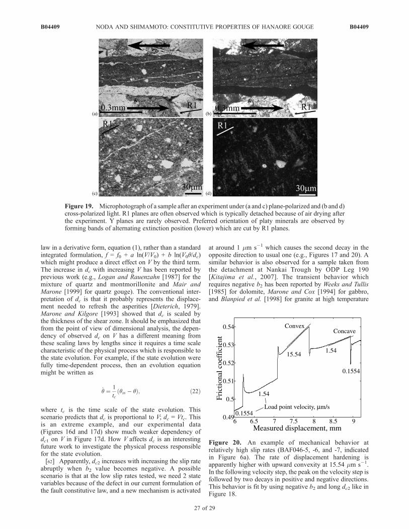
law in a derivative form, equation (1), rather than a standardintegrated formulation, f = f0 + a ln(V/V0) + b ln(V0q/dc)which might produce a direct effect on V by the third term.The increase in dc with increasing V has been reported byprevious work (e.g., Logan and Rauenzahn [1987] for themixture of quartz and montmorillonite and Mair andMarone [1999] for quartz gouge). The conventional inter-pretation of dc is that it probably represents the displace-ment needed to refresh the asperities [Dieterich, 1979].Marone and Kilgore [1993] showed that dc is scaled bythe thickness of the shear zone. It should be emphasized thatfrom the point of view of dimensional analysis, the depen-dency of observed dc on V has a different meaning fromthese scaling laws by lengths since it requires a time scalecharacteristic of the physical process which is responsible tothe state evolution. For example, if the state evolution werefully time-dependent process, then an evolution equationmight be written as

_q ¼ 1

tcqss � qð Þ; ð22Þ

where tc is the time scale of the state evolution. Thisscenario predicts that dc is proportional to V; dc = Vtc. Thisis an extreme example, and our experimental data(Figures 16d and 17d) show much weaker dependency ofdc1 on V in Figure 17d. How V affects dc is an interestingfuture work to investigate the physical process responsiblefor the state evolution.[62] Apparently, dc2 increases with increasing the slip rate

abruptly when b2 value becomes negative. A possiblescenario is that at the low slip rates tested, we need 2 statevariables because of the defect in our current formulation ofthe fault constitutive law, and a new mechanism is activated

at around 1 mm s�1 which causes the second decay in theopposite direction to usual one (e.g., Figures 17 and 20). Asimilar behavior is also observed for a sample taken fromthe detachment at Nankai Trough by ODP Leg 190[Kitajima et al., 2007]. The transient behavior whichrequires negative b2 has been reported by Weeks and Tullis[1985] for dolomite, Marone and Cox [1994] for gabbro,and Blanpied et al. [1998] for granite at high temperature

Figure 19. Microphotograph of a sample after an experiment under (a and c) plane-polarized and (b and d)cross-polarized light. R1 planes are often observed which is typically detached because of air drying afterthe experiment. Y planes are rarely observed. Preferred orientation of platy minerals are observed byforming bands of alternating extinction position (lower) which are cut by R1 planes.

Figure 20. An example of mechanical behavior atrelatively high slip rates (BAF046-5, -6, and -7, indicatedin Figure 6a). The rate of displacement hardening isapparently higher with upward convexity at 15.54 mm s�1.In the following velocity step, the peak on the velocity step isfollowed by two decays in positive and negative directions.This behavior is fit by using negative b2 and long dc2 like inFigure 18.


27 of 29

B04409

under a hydrothermal condition. The physical process forthis effect is unclear, and may be different for rocks. Moreexperimental and observational studies are needed to un-derstand the physical processes which dominantly affect thefrictional constitutive behavior of the natural fault.

8. Conclusions

[63] Our detailed investigation of the biaxial frictionapparatus in Kyoto University (now moved to HiroshimaUniversity) showed that the machine stiffness has an un-certainty which is shown to be nonnegligible in determiningthe fault constitutive parameters. This effect is importantwhen the normalized state evolution distance, dc = dc/(a/k)is not much larger than unity. We thus adopted a method inwhich the machine stiffness is treated as one of the fittingparameters. Our numerical experiments show that the faultconstitutive parameters are successfully recovered with thismethod.[64] Frictional experiments on simulated fault with sub-

millimeter thick black clayey fault gouge of the HanaoreFault (smectite, mica, and quartz) are conducted. Thefriction coefficient ranges from 0.43 to 0.62 with progress-ing displacement hardening. The a � Sb value changesfrom negative to positive around slip rate of 0.1 mm s�1.The overall behaviors of friction coefficient and a � Sbagree with the previous work by Saffer and Marone [2003]for mixture of smectite and quartz.[65] A behavior with 2 state variables (positive b1 with

short dc1 and negative b2 with long dc2) is typicallyobserved at the velocity steps between 1.54 and 15.54 mms�1. The constitutive parameters are determined by numer-ical least squares fittings with the stiffness of the apparatusas one of the fitting parameters. Typically, 2 state variablesare required to explain the experimental behavior. The avalue is around 0.01, and not remarkably dependent on theslip rate. The b1 does not vary significantly, neither, but b2apparently decreases and becomes negative at around 1 mms�1 with increasing slip rate. The dc2 increases with slip ratewhen the negative b value appears. Note that it is always thecase that b1 > b2 and dc1 < dc2.[66] Optical microscope observations of samples after the

experiments shows a composite plane structure of R1 andbands of alternation of extinction position at high anglefrom R1. The poor development of Y planes may beconsistent with the previous study since the peak strengthat the initial yielding is not clear [Logan et al., 1992]. Ourlow slip rate experiments do not reproduce naturally ob-served microstructures.

[67] Acknowledgments. We appreciate the comments by C. Maroneand N. Beeler which improved the manuscript by far. We thank T. Mitchellfor checking the grammar and phrasing before submitting the final version.This work is supported by JSPS research fellowship DC1, 17.2149.

ReferencesAndrews, D. J. (2002), A fault constitutive relation accounting for thermalpressurization of pore fluid, J. Geophys. Res., 107(B12), 2363,doi:10.1029/2002JB001942.

Bizzarri, A., and M. Cocco (2006a), A thermal pressurization model for thespontaneous dynamic rupture propagation on a three-dimensional fault: 1.Methodological approach, J. Geophys. Res., 111, B05303, doi:10.1029/2005JB003862.

Bizzarri, A., and M. Cocco (2006b), A thermal pressurization model for thespontaneous dynamic rupture propagation on a three-dimensional fault: 2.

Traction evolution and dynamic parameters, J. Geophys. Res., 111,B05304, doi:10.1029/2005JB003864.

Blanpied, M. L., C. J. Marone, D. A. Lockner, J. D. Byerlee, and D. P. King(1998), Quantitative measure of the variation in fault rheology due tofluid-rock interactions, J. Geophys. Res., 103(B5), 9691 – 9712,doi:10.1029/98JB00162.

Bos, B., and C. J. Spiers (2002), Fluid-assisted healing processes in gouge-bearing faults: Insights from experiments on a rock analogue system,Pure Appl. Geophys., 159, 2537–2566, doi:10.1007/s00024-002-8747-2.

Bos, B., C. J. Peach, and C. J. Spiers (2000), Frictional-viscous flow ofsimulated fault gouge caused by the combined effects of phyllosilicatesand pressure solution, Tectonophysics, 327, 173 –194, doi:10.1016/S0040-1951(00)00168-2.

Chester, F. M. (1994), Effects of temperature on friction: Constitutive equa-tions and experiments with quartz gouge, J. Geophys. Res., 99(B4),7247–7261, doi:10.1029/93JB03110.

Chester, F. M., M. Friedman, and J. M. Logan (1985), Foliated cataclasites,Tectonophysics, 111, 139–146, doi:10.1016/0040-1951(85)90071-X.

Chester, J. S., A. K. Kronenberg, F. M. Chester, and R. N. Guillemette(2003), Characterization of natural slip surfaces relevant to earthquakemechanics, Eos Trans. AGU, 84(46), Fall Meet. Suppl., Abstract S42C-0185.

Dieterich, J. H. (1979), Modeling of rock friction: 1. Experimental resultsand constitutive equations, J. Geophys. Res., 84(B5), 2161– 2168,doi:10.1029/JB084iB05p02161.

Dieterich, J. H. (1981), Constitutive properties of faults with simulatedgouge, in Mechanical Behavior of Crustal Rocks, Geophys. Monogr.Ser., vol. 24, edited by N. L. Carter, J. M. Logan, and D. W. Stearns,pp. 103–120, AGU, Washington, D. C.

Di Toro, G., D. L. Goldsby, and T. E. Tullis (2004), Friction falls towardzero in quartz rock as slip velocity approaches seismic rates, Nature, 427,436–439, doi:10.1038/nature02249.

Di Toro, G., T. Hirose, S. Nielsen, G. Pennacchioni, and T. Shimamoto(2006), Natural and experimental evidence of melt lubrication of faultsduring ear thquakes, Science , 311 , 647 – 649, doi :10.1126/science.1121012.

Fehlberg, E. (1969), Low-order classical Runge-Kutta formulas with step-size control and their application to some heat transfer problems, NASATech. Rep., 315.

Han, R., T. Shimamoto, T. Hirose, J. H. Ree, and J. Ando (2007), Ultra-lowfriction of carbonate faults caused by thermal decomposition during seis-mic slip, Science, 316, 878–881, doi:10.1126/science.1139763.

Hirose, T., and M. Bystricky (2007), Extreme dynamic weakening of faultsduring dehydration by coseismic shear heating, Geophys. Res. Lett., 34,L14311, doi:10.1029/2007GL030049.

Hirose, T., and T. Shimamoto (2005), Growth of molten zone as a mechan-ism of slip weakening of simulated faults in gabbro during frictionalmelting, J. Geophys. Res., 110, B05202, doi:10.1029/2004JB003207.

Hori, T., N. Kato, K. Hirahara, T. Baba, and Y. Kaneda (2004), A numericalsimulation of earthquake cycles along the Nankai trough, southwest Ja-pan: Lateral variation in frictional property due to the slab geometrycontrols the nuclear ion position, Earth Planet. Sci. Lett., 228, 215–226, doi:10.1016/j.epsl.2004.09.033.

Hoskins, E. R., J. C. Jaeger, and K. J. Rosengren (1968), A medium-scaledirect friction experiment, Int. J. Rock Mech. Min. Sci., 5, 143–154,doi:10.1016/0148-9062(68)90030-2.

Kawamoto, E., and T. Shimamoto (1997), Mechanical behavior of haliteand calcite shear zones from brittle to fully plastic deformation and arevised fault model, in Proceedings of the 30th International GeologicalCongress: Beijing, China, 4–14 August 1996, vol. 14, Structural Geol-ogy and Geomechanics, edited by Y. Zheng, G. A. Davis, and A. Yin, pp.89–105, VSP, Utrecht, Netherlands.

Kawamoto, E., and T. Shimamoto (1998), The strength profile for bimi-neralic shear zones: An insight from high-temperature shearing experi-ments on calcite-halite mixtures, Tectonophysics, 295, 1 – 14,doi:10.1016/S0040-1951(98)00112-7.

Kitajima, H., H. Noda, F. M. Chester, and T. Shimamoto (2007), Hydraulicand frictional properties of natural clay-rich sediments from ODP Leg190Nankai Trough and IODP Expedition 311 Cascadia Margin, Eos Trans.AGU, 88(52), Fall Meet. Suppl., Abstract S21B-0569.

Lachenbruch, A. H. (1980), Frictional heating, fluid pressure, and the re-sistance to fault motion, J. Geophys. Res., 85(B11), 6097 – 6122,doi:10.1029/JB085iB11p06097.

Lapusta, N., and J. R. Rice (2003), Nucleation and early seismic propaga-tion of small and large events in a crustal earthquake model, J. Geophys.Res., 108(B4), 2205, doi:10.1029/2001JB000793.

Lapusta, N., J. R. Rice, Y. Ben-Zion, and G. Zheng (2000), Elastodynamicanalysis for slow tectonic loading with spontaneous rupture episodes onfaults with rate- and state-dependent friction, J. Geophys. Res., 105(B10),23,765–23,789, doi:10.1029/2000JB900250.


28 of 29

B04409

Logan, J. M., and K. A. Rauenzahn (1987), Frictional dependence of gougemixtures of quartz and montmorillonite on velocity, composition andfabric, Tectonophysics, 144, 87 – 108, doi:10.1016/0040-1951(87)90010-2.

Logan, J. M., C. A. Dengo, N. G. Higgs, and Z. Z. Wang (1992), Fabrics ofexperimental fault zones: Their development and relationship to mechan-ical behavior, in Fault Mechanism and Transport Properties of Rocks,edited by B. Evans and T.-F. Wong, pp. 33–67, Academic, London.

Mair, K., and C. Marone (1999), Friction of simulated fault gouge for awide range of velocities and normal stresses, J. Geophys. Res., 104(B12),28,899–28,914, doi:10.1029/1999JB900279.

Marone, C. (1998), The effect of loading rate on static friction and the rateof fault healing during the earthquake cycle, Nature, 391, 69 – 72,doi:10.1038/34157.

Marone, C., and B. Kilgore (1993), Scaling of the critical slip distance forseismic faulting with shear strain in fault zones, Nature, 362, 618–621,doi:10.1038/362618a0.

Marone, C., C. B. Raleigh, and C. H. Scholz (1990), Frictional behaviorand constitutive modeling of simulated fault gouge, J. Geophys. Res.,95(B5), 7007–7025, doi:10.1029/JB095iB05p07007.

Marone, V., and S. J. Cox (1994), Scaling of rock friction constitutiveparameters: The effect of surface roughness and cumulative offset onfriction of gabbro, Pure Appl. Geophys., 143, 359–385, doi:10.1007/BF00874335.

Mase, C. W., and L. Smith (1985), Pore-fluid pressures and frictionalheating on a fault surface, Pure Appl. Geophys., 122, 583 – 607,doi:10.1007/BF00874618.

Mase, C. W., and L. Smith (1987), Effects of frictional heating on thethermal, hydrologic, and mechanical response of a fault, J. Geophys.Res., 92(B7), 6249–6272, doi:10.1029/JB092iB07p06249.

Mizoguchi, K., and T. Shimamoto (2004), Dramatic slip weakening ofNojima fault gouge at high-velocities and its implication for dynamicfault motion, Eos Trans. AGU, 85(47), Fall Meet. Suppl., AbstractT23A-0559.

Mizoguchi, K., T. Hirose, T. Shimamoto, and E. Fukuyama (2007), Recon-struction of faulting by high-velocity friction experiments: An example ofthe 1995 Kobe earthquake, Geophys. Res. Lett., 34, L01308, doi:10.1029/2006GL027931.

Morrow, C. A., D. E. Moore, and D. A. Lockner (2000), The effect ofmineral bond strength and absorbed water on fault gouge frictionalstrength, Geophys. Res. Lett., 27(6), 815 – 818, doi:10.1029/1999GL008401.

Nakae, S., and T. Yoshioka (1998), Geology of Kumakawa district, withgeological sheet map at 1:50,000 (in Japanese with English abstract),71 pp., Geol. Surv. Jpn., Tsukuba.

Nakatani, M. (2001), Conceptual and physical clarification of rate- andstate-dependent friction law: Frictional sliding as a thermally activatedrheology, J. Geophys. Res., 106, 13,347 – 13,380, doi:10.1029/2000JB900453.

Nielsen, H. B. (1999), Damping parameter in Marquardt’s method, Rep.IMM-REP-1999-05, 31 pp., Dep. of Math. Model., Technical Univ. ofDenmark, Lyngby.

Nielsen, S., G. Di Toro, T. Hirose, and T. Shimamoto (2008), Frictionalmelt and seismic slip, J. Geophys. Res., 113, B01308, doi:10.1029/2007JB005122.

Niemeijer, A. R., and C. J. Spiers (2006), Velocity dependence of strengthand healing behavior in simulated phyllosilicate-bearing fault gouge,Tectonophysics, 427, 231–253, doi:10.1016/j.tecto.2006.03.048.

Noda, H. (2008), Frictional constitutive law at intermediate slip rates ac-counting for flash heating and thermally activated slip process, J. Geo-phys. Res., 113, B09302, doi:10.1029/2007JB005406.

Noda, H., and T. Shimamoto (2005), Thermal pressurization and slip-weakening distance of a fault: An example of Hanaore Fault, southwestJapan, Bull. Seismol. Soc. Am., 95, 1224 – 1233, doi:10.1785/0120040089.

Ohnaka, M. (1973), Experimental studies of stick-slip and their applicationto the earthquake source mechanism, J. Phys. Earth, 21, 285–303.

Reinen, L. A., and J. D. Weeks (1993), Determination of rock frictionconstitutive parameters using an iterative least square inversion method,J. Geophys. Res., 98(B9), 15,937–15,950, doi:10.1029/93JB00780.

Reinen, L. A., T. E. Tullis, and J. D. Weeks (1992), Two mechanism modelfor frictional sliding of serpentinite, Geophys. Res. Lett., 19(15), 1535–1538, doi:10.1029/92GL01388.

Reinen, L. A., J. D. Weeks, and T. E. Tullis (1994), The frictional behaviorof lizerdite and antigorite serpentinies: Experiments, constitutive models,and implications for natural faults, Pure Appl. Geophys., 143, 317–358,doi:10.1007/BF00874334.

Research Group for Active Faults of Japan (1992),Maps of Active Faults inJapan With an Explanatory Text, Univ. of Tokyo Press, Tokyo.

Rice, J. R. (2006), Heating and weakening of faults during earthquake slip,J. Geophys. Res., 111, B05311, doi:10.1029/2005JB004006.

Rice, J. R., N. Lapusta, and K. Ranjith (2001), Rate and state dependentfriction and the stability of sliding between elastically deformable solids,J. Mech. Phys. Solids, 49, 1865–1898.

Ruina, A. L. (1983), Slip instability and state variable friction laws,J . Geophys. Res . , 88 (B12) , 10,359 – 10,370, doi :10.1029/JB088iB12p10359.

Saffer, D. M., and C. Marone (2003), Comparison of smectite- and illite-rich gouge frictional properties: Application to the updip limit of theseismogenic zone along subduction megathrusts, Earth Planet. Sci. Lett.,215, 219–235, doi:10.1016/S0012-821X(03)00424-2.

Segall, P., and J. R. Rice (1995), Dilatancy, compaction, and slip instabilityof a fluid-infiltrated fault, J. Geophys. Res., 100(B11), 22,155–22,171,doi:10.1029/95JB02403.

Shibazaki, B., N. Shigematsu, and H. Tanaka (2004), Modeling slip andnucleation processes at the deeper part of the seismogenic zone, EarthPlanets Space, 56, 1087–1093.

Shimamoto, T. (1986), Transition between frictional slip and ductile flowfor halite shear zones at room temperature, Science, 231, 711–714,doi:10.1126/science.231.4739.711.

Shimamoto, T., J. W. Handin, and J. M. Logan (1980), Specimen-apparatusinteraction during stick-slip in a triaxial compression machine: A de-coupled two-degree-of-freedom model, Tectonophysics, 67, 175–205,doi:10.1016/0040-1951(80)90234-6.

Shimamoto, T., A. Tsutsumi, T. Hirose, Y. Aizawa, H. Sone, S. Uehara,W. Tanikawa, H. Noda, and K. Mizoguchi (2006), Friction, deformationand fluid-flow apparatus at Kyoto Univ. (in Japanese with Englishabstract), Jpn. J. Struct. Geol., 49, 49–71.

Sibson, R. H. (1973), Interaction between temperature and pore-fluid pres-sure during earthquake faulting—A mechanism for partial or total stressrelief, Nature, 243, 66–68.

Sirono, S., K. Satomi, and S. Watanabe (2006), Numerical simulations offrictional melting: Small dependence of shear stress drop on viscosityparameters, J. Geophys. Res., 111, B06309, doi:10.1029/2005JB003858.

Togo, M., H. Sato, T. Shimamoto, A. Tsutsumi, S. Ma, and T. Nakamura(1997), On the latest paleoseismic event of the Hanaori fault near Kyoto,central Japan (in Japanese with English abstract), Active Fault Res., 16,44–52.

Tse, S. T., and J. R. Rice (1986), Crustal earthquake instability in relation tothe depth variation of frictional slip properties, J. Geophys. Res., 91(B9),9452–9472, doi:10.1029/JB091iB09p09452.

Tsutsumi, A., and T. Shimamoto (1997), High velocity frictional propertiesof gabbro, Geophys. Res. Lett., 24(6), 699 – 702, doi:10.1029/97GL00503.

Tullis, T. E., and D. L. Goldsby (2003), Laboratory experiments on faultshear resistance relevant to coseismic earthquake slip, SCEC AnnualProgress Report 2003, South. Calif. Earthquake Cent., Los Angeles.

Tullis, T. E., and J. D. Weeks (1986), Constitutive behavior and stability offrictional sliding of granite, Pure Appl. Geophys., 124, 383 –414,doi:10.1007/BF00877209.

Weeks, J. D., and T. E. Tullis (1985), Frictional sliding of dolomite: Avariation in constitutive behavior, J. Geophys. Res., 90(B9), 7821–7826, doi:10.1029/JB090iB09p07821.

Wibberley, C. A. J., and T. Shimamoto (2005), Earthquake slip weakeningand asperities explained by thermal pressurization, Nature, 436, 689–692, doi:10.1038/nature03901.

Yoshioka, T., Y. Kariya, F. Nanayama, A. Okada, and K. Takemura (1998),Latest faulting of the Hanaore fault, central Japan, revealed by trenchingstudies, and the 1662 Kambun earthquake (in Japanese with Englishabstract), J. Seismol. Soc. Jpn., 51, 83–97.

Yoshioka, T., A. Cho, K. Kimura, and S. Nakae (2000), Explanatory text ofthe strip map of the Hanaore fault, central Japan (in Japanese with Eng-lish abstract), Tectonic Map Ser. 13, scale 1:25,000, 35 pp., Geol. Surv.Jpn., Tsukuba.

��H. Noda, Seismological Laboratory, California Institute of Technology,

1200 E. California Boulevard, Mail Code MS 252-21, Pasadena, CA 91125,USA. ([email protected])T. Shimamoto, Department of Earth and Planetary Systems Science,

Graduate School of Science, Hiroshima University, Higashi-Hiroshima739-8526, Japan.


29 of 29

B04409

constitutive properties of clayey fault gouge from the ... · constitutive properties of clayey...

Documents